Fatigue and Stochastic Loads_RYCHLIK

7/15/2019 Fatigue and Stochastic Loads_RYCHLIK

http://slidepdf.com/reader/full/fatigue-and-stochastic-loadsrychlik 1/19

Board of the Foundation of the Scandinavian Journal of Statistics

Fatigue and Stochastic LoadsAuthor(s): Igor RychlikSource: Scandinavian Journal of Statistics, Vol. 23, No. 4 (Dec., 1996), pp. 387-404Published by: Wiley on behalf of Board of the Foundation of the Scandinavian Journal of Statistics

Stable URL: http://www.jstor.org/stable/4616416 .Accessed: 08/07/2013 09:50

Your use of the JSTOR archive indicates your acceptance of the Terms & Conditions of Use, available at .http://www.jstor.org/page/info/about/policies/terms.jsp

.JSTOR is a not-for-profit service that helps scholars, researchers, and students discover, use, and build upon a wide range of

content in a trusted digital archive. We use information technology and tools to increase productivity and facilitate new forms

of scholarship. For more information about JSTOR, please contact [email protected].

.

Wiley and Board of the Foundation of the Scandinavian Journal of Statistics are collaborating with JSTOR to

digitize, preserve and extend access to Scandinavian Journal of Statistics.

http://www.jstor.org

This content downloaded from 194.210.224.251 on Mon, 8 Jul 2013 09:50:07 AMAll use subject to JSTOR Terms and Conditions

http://www.jstor.org/action/showPublisher?publisherCode=black

http://www.jstor.org/action/showPublisher?publisherCode=bfsjs

http://www.jstor.org/stable/4616416?origin=JSTOR-pdf

http://www.jstor.org/page/info/about/policies/terms.jsp





http://www.jstor.org/stable/4616416?origin=JSTOR-pdf

http://www.jstor.org/action/showPublisher?publisherCode=bfsjs

http://www.jstor.org/action/showPublisher?publisherCode=black



? Board of the Foundation of the Scandinavian Journalof Statistics 1996. Published by Blackwell Publishers Ltd., 108Cowley Road,

Oxford OX4 IJF, UK and 238 Main Street, Cambridge, MA 02142, USA. Vol. 23: 387-404, 1996

Fatigue and Stochastic Loads*

IGOR RYCHLIKUniversity of Lund

ABSTRACT. We give a general introductionto fatigue and discuss a simple model of fatigue

damage accumulation in metals under variable loading conditions. Loads are modelled as

stochastic processes and importantcharacteristics of loads' variability, relevant for fatigue, are

presented.We also discuss methods to generate loads for fatigue tests.

Key words: crossings, fatigue, local extremes, oscillation measures, rainflow cycles

1. Introduction

Fatigue is a process of "ageing" or "degrading" of materials, mostly metals, in components

and structures subjected to time-variable external loading conditions. The fatigue process

causes the deterioration of the material's ability to carry the intended load. It is a common

opinion among reliability engineers that failure of mechanical components in most cases is

caused by fatigue.

Fatigue has been the subject of numerous research studies conducted by mechanical

engineers, material scientists, physicists, chemists, structural engineers and mathematicians

over more than 150 years. The complexity of the fatigue process and related reliability

problems requires development of new statistical tools for analysing fatigue data, design of

experiments and tests. One also needs reliable stochastic models for materials properties,

environment variability and for uniaxial and multiaxial loads. At present such models use i.a.

random morphology, integral geometry, point processes, Gaussian processes and stochastic

differential equations.

In this paper we review an approach to fatigue under random loading conditions based on

a concept of a macroscopic damage accumulations in the material, see also Sobczyk (1987)

and Miller (1993). Modelling of crack development is not considered and we refer to a

monograph by Sobczyk & Spencer (1992).

2. Fatigue

The fatigue phenomenon is a very complicated process which can be defined as a process ofnucleation (or crack initiation) and crack growth when some cracks stop growing while

others collapse and create long cracks. The growth rate increases with the crack length, even

under small variable loading. Due to surface imperfections, inclusions, grain boundaries etc.,

initiation of cracks usually takes place at the surface of the metallic body at spots of high

stress concentration.

Depending on the magnitude of the load, the properties of the material, and the

smoothness of the surface, the crack nucleation phase may constitute the main part of the

total fatigue life or, in other cases, it may be completely absent. This means that fatigue

failure is directly a result of the crack growth process. Summarizing, the fatigue damage

process is very complicated and depends on many factors:

* This paper was presented as an Invited Lecture at the 15th Nordic Conference on Mathematical

Statistics, Lund, Sweden, August 1994.







388 I. Rychlik Scand J Statist 23

(a) the micro-structure of the material: the crystal size and geometry distribution of

inclusions, surface finish, etc.;

(b) the variability of applied loads as well as the geometry and dimensions of the object,

notches, etc.; and

(c) the environmental conditions, such as aggressive chemical environment leading to

corrosion, large temperature variations, etc.,

see Miller (1993) for more detailed discussion. It is obvious, from the complexity of the

fatigue phenomena that observed life times to failure have a considerable variation.

The first systematic and quantitative investigation of fatigue damage was performed by

August Wohler in 1858 and resulted in the widely known Wohler curve, or S-N diagram,

which shows the relationship between the amplitude (S) of the applied (approximatively

sinusoidal) stress function and the number (N) of periods to fatigue failure. The S-N

diagram is an important measure of material strength for fatigue.

Assume that we have a set of test specimens produced so that maximal homogeneity of thespecimens' shape and surface is achieved. Let all the specimens be subjected to an oscillatory

load y, where y may represent a stress or elongation function. For simplicity we assume that

the function y is a sinusoid function,

Sy, = m + - sin (27rAt), 0 <t <,,

where r is the time of failure.

In practical tests one sometimes uses other shapes of the periodic "cycles" constituting y

than the sinusoidal. However, it has been observed that the particular shape of the function

is of secondary importance compared to the period, maximum and minimum value of theoscillatory load. Thus the parameters u = max y, and v = min yt can be used as parameters

of the simple oscillatory load, also called constant amplitude load.

Although the specimens are almost identical and the loading function y is the same for all

specimens, one often observes a large variability in life times T,which is due to randomness

of material properties. In fatigue analysis one equivalently uses sn(v, u) = T i, the number of

cycles to failure or time to failure T,as a measure of materials strength. In order to identify

the properties of sn(v, u) one has to perform fatigue tests for different values of (v, u). It is

a common experience that the values of sn(v, u) closely follow a log normal distribution.

Further, one often assumes, in contrast to most observations, that the variance of ln (sn(v, u))

is independent of (v, u). Consequently, a simple regression model for the strength process

sn(v, u) is the following one:

sn(v, u) = K SN(v, u), K = exp (aX) (1)

where X e N(O, 1) and SN(v, u) is a deterministic strength function, which is equivalent to the

S-N diagram. In practical codes (or specifications) one often fits a simple form for SN(v, u)

SN(v, u) = SN(u -v) = {k(u -v)J if u-v >,so, (2){k (u - v) if u - v < so,

where /B a t 1 and kI = k(so) - if ,B< oo. If ,B= oo the amplitude so is called the fatigue

limit and means that a load with amplitude u-

v < so does not cause any fatigue damage.Relatively standard techniques from regression analysis can be used to estimate the parame-

ters k, a, fJ,so and a. However, since fatigue experiments are very expensive, one usually has

rather small sets of data and hence the design of experiment is important.

? Board of the Foundation of the Scandinavian Journal of Statistics 1996.







Scand J Statist 23 Fatigue and stochastic loads 389

2.1. Fatigue damage

In the previous section we have used a simple constant amplitude load y (for example a

sinusoidal function). Obviously real loads are seldom so regular. Consequently we need to

find methods to characterize variability of a load relevant for fatigue life prediction.The approach presented here is based on a concept of accumulation of damage in a

material due to fatigue phenomena. Although it is difficult to define how to measure

(physically) fatigue damage, the concept of damage has physical meaning and should be

related to the collection of cracks in the material. This is indicated by experiments where a

thin layer of the surface was periodically removed from a fatigued specimen (thereby

eliminating the early stages of short crack growth). Tests of such renovated specimens at the

same stress-strain level indicate that no damage has been introduced into the bulk of the

material, neglecting the changes in the response to a load, because full life time has been

restored.

Here we shall present a linear damage accumulation model proposed by Palmgren (1924)and Miner (1945). This approach is commonly used in engineering practice.

We begin with the damage intensity for a constant amplitude load function y, i.e. a

periodic function, with frequency i, and such that in a period it has only one local minimum

with height v and one local maximum with height u. On a unit scale, a damage intensity is

defined as d, = A/SN(v, u), where SN(v, u) is a standard strength of a specimen obtained from

the S-N diagram. The total damage accumulated in the interval [0, T] is defined as

bT

DT= dtdt,

and the fatigue failure time-

has distribution given by P(T S t) = P(Dt > K), where K is arandom critical level; see (1).

Before we give a general form of the Palmgren-Miner damage accumulation model we

present a physical motivation for the method. It is generally accepted that elastoplastic

deformations cause damage to material. A large enough deformation destroys a given piece

of material immediately, while smaller deformations lead to eventual destruction if they are

applied repeatedly. Thus a single hysteresis loop in the stress-strain plane constitutes a basic

event for damage assessments. In the simplest models the order of the hysteresis loops is

neglected and damage is attached to each single hysteresis loop. Then the total damage is

defined as a sum of damages attached to all closed hysteresis loops.

The hysteresis loops can be easily identified in a graph of the (stress, strain)-function. The

(stress, strain)-functions are sometimes measured in fatigue experiments, particularly if there

are regions where plastic deformations can be significant, e.g. in notched components.

However, it is a common situation in the design stage of a construction or in a fatigue life

prediction that only external loadings are known and that the stress/strain-relations need to

be approximated using numerical algorithms. Consequently, the stress function alone is often

used both to identify hysteresis cycles and to attach damages to cycles.

Let v, u be the lowest and highest points of a hysteresis loop on a stress axis and let the

damage attached to the loop be denoted byf(v, u). The total damage DT accumulated in the

time interval [0, T] is then a sum of damages attached to all closed hysteresis loops {(vi, ui)},say, in [0, T], i.e.

DT = Zf(vi, ui). (3)

Using a constant amplitude fatigue life data (S-N curve) we can calibrate the total damage









and obtain the general Palmgren-Miner linear damage accumulation law

DT= SN(vZ U P(T < t) =P(Dt > K). (4)

The remaining problem is to identify the lowest and highest points of a hysteresis loop on a

stress axis of closed hysteresis loops {(vi, ui)} given the stress function y. The so-called

rainflow method is a method to do this, as described in the following section.

The most critical assumption in the Palmgren-Miner model is that the damage of the ith

cycle is independent of the magnitudes of other cycles. There are many experiments

disclosing sequential effects, e.g. the fact that the crack grows slower after an overload.

However, there is no general damage accumulation method which can take into account all

sequential effects and which is uniformly better than other approaches. Consequently, if the

sequential effects are not dominating the damage accumulation process, the simplest ap-

proach of Palmgren and Miner is still frequently used in engineering practice. In addition,

some engineers interpret the rainflow count as a method to introduce sequential effects

(through hysteresis memory of a material) into the Palmgren-Miner damage accumulation

model. This is then used to explain the relatively good accuracy in fatigue life prediction

based on the rainflow method and the Palmgren-Miner damage, i.e. using equations (4).

Furthermore, note that in material science, there is and has been an intensive discussion on

whether and how the energy dissipated in a material during elastoplastic loading and the

accumulated fatigue damage are related to each other. Brokate et al. (1994) showed that

both energy dissipated in the material and the Palmgren-Miner fatigue damage (4) can be

described using the so-called hysteresis operators with a set of rainflow cycles as a basic

component. Consequently the energy dissipated in a material can be well-approximated by

formula (3) with (may be) a different function f than in (4).

3. Rainflow count, basic properties

The rainflow method was introduced by Endo in the late sixties, the first paper in English

being Matsuishi & Endo (1968). The original paper in Japanese has been reprinted in

Murakami (1992). His definition was a complicated recursivealgorithm identifying the closed

hysteresis loops in the strain-stress plane. Endo described the method using a model of rain

flowing from a pagoda roof (which explains the name). The first non-recursive definition of

the method was given in Rychlik (1987).

Definition 1

Let CT,0 < T < oo, be a space of continuous real functions defined on [0, T]. For y E CT,

define a real function x by the following procedure:

For any fixed t E[0, T] let t -, t + be the following time points

_ usU C- 0, t):Y S>Yt }o

lo if ys < yt for all sE [0, t),

+ Jinf Is E (t, T): ys>

y, },

}T if ys <y for all s e (t, T)

and let x , x + be the lowest points in the intervals [t-, t], [t, t +], respectively, i.e.

Boardf th nyd:i- < s < te,xS + = infyr: t < s <a+t (6)








Xt t

t- ~~t t+

Fig. 1. Definitionof rainflow ycle.

then x, is given by

Smax(x,<x+) ift+ < Toryt =YT and t < T, (7)

lx= otherwise,

see Fig. 1. A function rfc = (rfc, = (xt, yt), t E [0, T]), will be called a rainflow unction of y

and a pair (xt, yt) such that xt <Yt is called a rainflow cycle originating at t, with top yt,

bottom x,.

We turn now to the damage DT defined by (4); for a positive function f(v, u) > 0, v < u,

a damage functional is given by

y -+DT(f) =E f(rfct)l{(x,y):x<y}(rfct), (8)

t e [0, T]

where lA(X) = 1 if x c A and zero otherwise. In what follows we shall equivalently use the

notation DT, DT(f) or D(f; y). In practice ft(v, u) = 1/N(v, u), where N(v, u) is a S-N

curve. Using the S-N curve (2) with ,B= oo and fatigue limit s0 >0 the total damage

becomes

Dt k Z (y'-x Y',

Yt- Xt -> So

where a and k are material dependent constants (k is usually very large).

Given an observed load y and a S-N curve it is a straightforward task to compute the

total damage DT using the rainflow algorithm, given in definition 1, and (8). However, let e.g.

y be a measurement of a stress at a fixed point of a truck travelling between locations A and

B, say. Obviously, y can not be reproduced by a new measurement and it seems natural to

model y as a sample path of a stochastic process.Now, if y is modelled by a stochastic process the important question is how to compute

expected damage, its variance or a distribution function given the law of y. Since the rainflow

function rfc depends in a very complicated way on y, (8) is not very convenient for stochastic

analysis of DT. In the following two subsections we shall represent a rainflow function as a

point process in R2 and describe it using a counting distribution, i.e. a number of points in

a suitable class of subsets of R2. Next the total damage DT will be written in a form of an

integral of the counting distribution. Since the counting distribution is equal to a number of

upcrossings of an interval by y (the same as used in Doob's upcrossing lemma for

supermartingales) the computation of expected damage is more tractable.

3.1. Countingdistribution

We begin with a simple lemma.

? Boardof the Foundation f the Scandinavianournalof Statistics1996.








Lemma 1

For y E CT, T < ?O, the number of times the rainflow amplitude is at least e > 0, i.e.

NT(E) = #{t E [0, T]:y t-xt > }, (9)

is finite.

By lemma 1, the set rfc(y) = {(x,, yt): Yt> xt, t E [0, T]} is countable (and measurable),

hence it is a point process in {(v, u): v < u}. The set will be called a rainflowcount. A rainflow

count can be uniquely defined using its counting distribution

NT(V, U) = # {t E [O,T]: v, uE [xt, y,]}, v < u. (10)

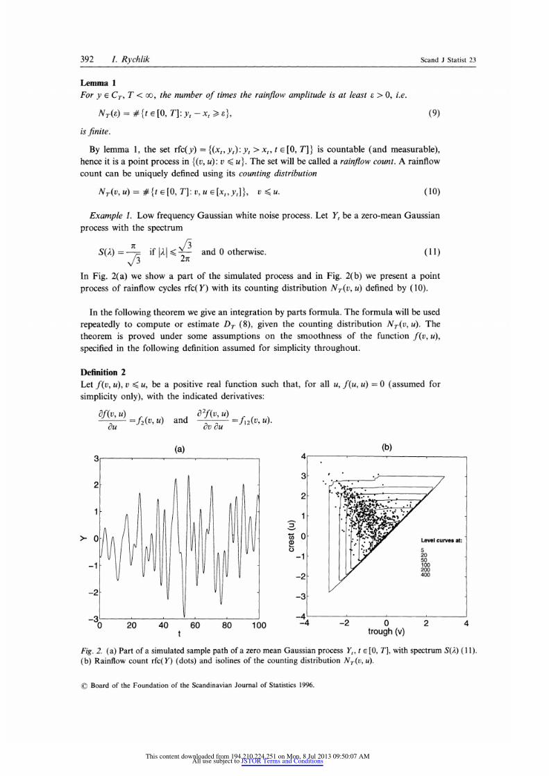
Example 1. Low frequency Gaussian white noise process. Let Y, be a zero-mean Gaussian

process with the spectrum

S(i) = if JA2< and 0 otherwise. (11)

In Fig. 2(a) we show a part of the simulated process and in Fig. 2(b) we present a point

process of rainflow cycles rfc(Y) with its counting distribution NT(V, u) defined by (10).

In the following theorem we give an integration by parts formula. The formula will be used

repeatedly to compute or estimate DT (8), given the counting distribution NT(V, u). The

theorem is proved under some assumptions on the smoothness of the function f(v, u),

specified in the following definition assumed for simplicity throughout.

Definition 2Let f(v, u), v < u, be a positive real function such that, for all u, f(u, u) = 0 (assumed for

simplicity only), with the indicated derivatives:

af(v,u) a02fv U)afu) =f2(v, u) and

A=f2(v,u).Au avAu

(a) (b)

3~~~~~~~~~~~~

2

1~~~~~~~~~~~~

>0 ~~~~~~~~~~~~~~~~urves at:

0~~~~~~~~~~~2-1~~~~~~~~~~5

-100; lS tdyX 0 BR! 1

-2 ~ ~ ~ ~ ~ ~ ~ ~ ~~~--2 ~~~~~~~~~~~3-

-o 20 40 60 80 100 -2 02 4

t trough (v)

Fig. 2. (a) Part of a simulated sample path of a zero mean Gaussian process Y, t E [0, T], with spectrum S(i) (11).

(b) Rainflow count rfc(Y) (dots) and isolines of the counting distribution NA(V U).









Assume that for all u e R, f2(u, u) ) 0 is a continuous function of u, and for all v < u,

f12(v, u) < O. If for all x < z

Cz ru

J

{I (V, U)I dvdu < ,

ox x

then f will be called a damage function.

The following theorem gives an integration by parts formula to compute the total damage

DT-

Theorem 1

For y E CT, let NT(V, u) be its rainflow counting distribution,defined by (10), and let f be a

damage function (see definition 2). Then the total damage DT is given by

DT - NT(V, u)fI2(V, u)dvdu+ NT(U, u)f2(u, u)du. (12)%V<U R

Note that in the proof of (12) only the integrability of the second derivativef12is needed.

The additional assumptions that f2(u, u) > 0 and that f12(v, u) s< 0, imposed in definition 2,

ensure that the damage DT is a non-decreasing function of T for any continuous y. The

continuity of DT will be discussed in subsection 3.5.

The case when f(v, u) = (u - v)c, a ? 1, is of special interest. We then refer to DT(ft) as

the oc-damage.From the last theorem it follows that

DT(f') = N U(u,u) du, DT(f) = 2 NT(V, u) dv du.,R 0 V-<U

For c-damage, the integration by parts formula (12) can be simplified by considering NT(h),

defined by (9), instead of NT(V, U), since then

DT(ft) = oc h NT(h) dh. (13)

3.2. Rainflow count and oscillation measure

In the previous subsection we have defined a rainflow function (t, y) -+ rfc5, and used it to

evaluate the damage functional DT through (8). Since the rainflow function depends in a

complicated way on y, this approach is inconvenient if one wishes to study the dependence

of DT on time T. An alternative way is to use integration by parts formulas (12) or (13) to

compute DT and determine how NT(V, u) and NT(h) depend on T. This approach is only

meaningful if one can find an alternative way to compute NT(V, u) and NT(h) than by (10)

and (9), respectively. A proof of the following characterization of NT(V, U), V < u, can be

found in Rychlik (1993),

NT(V, U) = number of passages from v to u by y in [0, T],

which is made precise in the following lemma. Scheutzow (1994) proves this relationship for

regular functions, e.g. cadlag functions. The relationship between crossings and rainflow

counting distribution has been worked out independently by a research team from TEC-

MATH in Kaiserslautern and the author, see papers 3 and 4 in Murakami (1992).









u ------ -- -

v----- ---- VW

I i i Ii

TO=O S1 T1 S2 T2

Fig. 3. Illustration of the first passage times Si, Ti, in lemma 2.

Lemma 2

For y E CT and any fixed levels v < u, define the sequence of first passage times, see Fig. 3,

To=0 and

S1 =inf{t ,0:yt =v}, T1=inf{t >S1:y, =u},

S2=inf{t > T,:yt =V}, T2=inf {t S2:Y, =U},

with the convention that inf {0}= + oc. Then

NT(V, U) = max {n: Tn< T}. (14)

Thefunction NT(V, U) = max {n: Tn< T} is called an oscillation measure.

The formulas (14) and (12) form the basis for computation of expected damage due

to rainflow cycles. In the special case of a-damage, i.e. f/(v, u) = (u - v) , a > 0, the

simpler formula (13) can be used. However, we need a computationally more convenientcharacteristic of NT(h) than the defining relation NT(h) = the number of rainflow cycles in

[0, T] with amplitude at least h. In Rychlik (1994) we gave a characterization of NT(h)

similar to (14).

3.3. Rainflow cycles and a sequence of turningpoints

As mentioned in section 1, usually, cycles with small amplitudes do not cause any damage,

e.g. so > 0 and ,B= oo in (2). Consequently, all cycles with small amplitude are often removed

from the observed load and the values of y are discretized. The procedure is called hysteresis

filtering. We shall now formalize this procedure mathematically.

For a fixed h > 0, let = f{y0+ ih: i = .. ., -1, 01, 2, . . .} be a set of levels. Define by

induction a sequence of first passage times {Tj : let T0= 0 and given Tj, let

u =inf{z E : z >y,j}, v =sup {z E1: z <yj4,

then

Tj+i =inf {t > tj:y, =u or Yt= v},

as before inf {0} = + oo. Consequently, zj,j > I, are the time points when y, passes the

discrete levels in W. Obviously, if T < oo then K = sup {j: Tj< T} < oo, since y is continuous.

Let 9 be an approximation of y obtained by drawing straight lines between points

{(TO,YT) . * (rK, YTK),(T, YT }-Further data reduction is obtained by deleting from { To'YT ).(TKZYTK), (T Y) } all

points (zi, y,,) which are not points of strict local extremes in y. The remaining sequence is

called the sequence of turning points, see the following definition.









Definition 3

Let {(ti, Mi)} I1, Mi = y.t, be the sequence of local maxima in 9. (If YTK YT, (T, YT) is

consideredas a point of local maximum.)Let to= 0 and definemi= inf {9t:ti -l < t <ti }

The sequence of pairs {(mi, Mi) lm is called a sequence of discretized turningpoints in y.

Applying he rainflowmethod o the sequenceof turningpointswe obtain thesequenceof

rainflow cycles {(mrfc, Mi }iMSince T < oo and y is a continuousfunction, sequencesof turningpoints and rainflow

cycles akefinitelymanyvalues romthe set 1.Consequently,heycan be uniquelydescribed

by means of bivariatehistogramsof (mi, Mi) and (mrfc, Mi) called in fatigue practice

Markov-respectivelyainflow-matricesnd whichare a commonway of savingthe observed

loads.

Denoteby NT(V, u) an oscillationmeasureof 9. (Obviously, AT(V, ) can be obtained rom

rainflowmatrix and vice-versa)by a simplealgebra.)The following emma ustifies he use

of rainflowmatriceso approximatehe rainflowdamageDT(Y) for a continuous unctiony.

Lemma 3

Let y ECT and 9 be its approximation defined in this subsection. Denote by NT(V, u) an

oscillation measure of 9, defined by (14) and let NT(V, u) be an oscillation measureof y. Then:

(a) For any u > v, NT(V, U) < NT(V, U) with equality when v, u E 1, (v < u).

(b) The numberNT(h) of rainflowamplitudesat least h counted in y is bounded rom below

by M, the numberof local maxima in 9, and NT(2h) < M < NT(h).

(c) For a damagefunction f, Dr(f; 9) TDT(f; y), (h - 2-n) as n -, oo.

3.4. Finiteness of rainflowdamage

If y has finitelymanyextremes hen the total damageDT is finitefor any damage unction.

Examplesof suchregularoadsare samplesof Gaussian ow frequencywhite noiseprocess

presentedn example1. Obviously, unctionsy of finitevariationmayhave infinitenumbers

of localextremesn [0, TI,seeexample2, but f, NT(U,U) dU S finite by Banach's heorem,

(see Freedman,1983,p. 209),and since it is assumed hat (u, u) = 0, for all u, the rainflow

damage s finite for all damage unctions, definedas in definition2.

Example2. Linear oscillator.Let Y, be the solution of a dampedharmonicoscillator

equationdrivenby a Gaussianwhite noise process, .e. let

Y','+2Yt + Y, = Wt, t >,0, (15)

where W, s a Gaussianwhite noiseprocess.Assumea' = 4Cand(Y0, Y0)= (XI,X2),where

Xi are independentN(0, 1) variables.Then Y, is a zero-mean tationaryGaussianprocesswith spectraldensity

a12Ry(A)=(1 -(2,%)2)2 + (2C)2(2ir))2

For the process Ytwe have (U2= U2, = 1. Consequently, lmost all sampleshave finite2-variation.However,sincea2,- oo, the processhas infinitelymanylocal extremes.

For the constantC= 0.01, in Fig. 4(a) we presenta partof a simulated, ampledprocessYk d whered = 0.005. Thefirst 100 ocalextremes remarkedas stars.Theplot on Fig. 4(b)showsthe rainflowcount rfc(Y)and we can see that most of the cyclesare along the line

y = x, i.e. haveverysmallamplitudes,wheredamage s negligible.








396 I. Rychlik ScandJ Statist23

(a) (b)

1.5

2 .

15 . ...

0.51

>- 0

-0.5-1

-1 -

-1.5 -

5 10 15 20 -f3 -2 -1 0 1 2t trough

Fig. 4. (a) Part of a simulated amplepath of a zero mean GaussianprocessYt,t E[0, 500],definedby (15), with

the first 100 local extremesmarkedas stars.(b) Rainflowcount rfc(Y) (dots).

If the function y has infinite variation then f NT(U, u) du = oo and, in order to avoid

pathological cases, we assume that f2(u, u) = 0 for all u E R. Under this assumption, using the

integral representation (12), the total damage is given by

"b "b- a

DT = { NT(U -h, u)f12(U -h, u) dh du,.a O0

where b = max, E[0 T] yt, a = mintE[OTj y,. Hence, in order to check if the total damage DT iS

finite we need to describe properties of the damage function f(v, U) for v close to u more

precisely, and limit the class of functions y.

For simplicity consider f(v, u) = (U - v) , o > 1. Then by ( 13) the total damage

b-a

DT(f;y) = f b ho INT(h)dh,

and NT(h) is the number of rainflow cycles in [0, T] with amplitudes at least h. Obviously,

the finiteness of DT depends on the growth rate of NT(h) as h tends to zero. This is exactly

the rate the number of local maxima M in lemma 3(b) grows as h tends to zero.

Theorem 2

Let Yt, t e [0, T], be a continuous Brownian motion starting at zero and

fl(v, u) = (u - v) ", 2 ) 1. Then the rainflowdamage DT( P; Y) is a.s. infinite or cx< 2 and a.s.

finite for oc> 2.

Example 3. Ornstein-Uhlenbeck process. Let Y, be a zero mean stationary Gaussian

process with covariance function r(t) = E[Yo Yt] = a2(2c) 1 exp { -c|t|}, c > 0. The Orn-

stein-Uhlenbeck process Y is extremely irregular, almost all samples have infinite variation

and the set of local maxima is countable and dense in [0, T], see also Fig. 5(a). Furthermore,NT(h) = O(h 2) as h tends to zero, and the oc-damage s infinite for ac< 2. (In the simulation

we used Y,t+= Ytexp{-ck31}+ X cr[(l-exp { -2c 6j})I(2c)]1/2, = 0.002, whereX is a

standard Gaussian variable independent of Y_,s < t.)

g Board of the Foundation of the Scandinavian Journal of Statistics 1996.








(a) (b)3

-0.5

2 -::.

0

-1.5

-2-2

0 0.5 1 1.5 2 =3 2 -1 0 1 2t trough

Fig. 5. (a) Part of a simulated amplepath of an Ornstein-Uhlenbeck rocess Y, 0 ? t ?200, with

parameters = 0.5, a = 1. (b) Rainflowcountrfc(Y)(dots).

3.5. The rainflow damage process

Let Yt, t E [0, + oo) be a continuous function. Obviously, for any finite T > 0 the function y

restricted to [0, T] is in CT and we can define the rainflow damage DT(f; y). Let DO= 0 and

let f be a damage function such that DT(f; y) < oo for all finite T then:

(i) DT is a continuous non-decreasing function.

(ii) DT is a Lipschitz continuous function, if yt is Lipschitz continuous (f(u, u) = 0 for all

u ER). Furthermore

rT ST

DT ={0 D'dt =jf2(x, yt)1{x x>o}(YD)Y;dt, (16)

where x- is defined as in definition 1.

Note that in the case when f(v, u)=

G(u)-

G(v) the total damage can be written inparticularly simple form DT =f-TG'(yt)1{x >o}(y)y dt.

4. Expected rainflow damage

Let Yt, t > 0, be a random process with a.s. continuous sample paths, f a damage function

(as in definition 2) and DT(f; Y) a rainflow damage process. In this section we study the

expectation E[DTI.

From (12), using Fubini's theorem, the necessary condition for finiteness of expected

damage is finiteness of measure

+ 00

nT (V, u) = E[NT(V, U)] = E P(Tn < T), ( 17)n= I

where the oscillation measure NT and first passage times Tnare defined in lemma 2. Then the









expected damage is given by

E[DT]= - T nT(v, u)fI2(v, u) dvdu + J'nT(u u)f2(u, u) u. (18)v_<u R

Since Tnare rather complicated first passage times we can not expect to find explicit forms

for nT(v, u) except for some special cases. Hence approximation methods are often used, see

Rychlik (1988). We begin with two important classes of processes when explicit forms do

exist.

4.1. Diffusion processes

Let Y,, t > 0, be a regular diffusion process on R with diffusion coefficient a(z) > 0 and drift

coefficient b(z). (The sample paths of Y are a.s. continuous and have infinite variation.) For

arbitrary x0 define

T'byr b(z)S(x)= exp -I dz dy,

Jxo { Jx0 a(z) }

the so-called scale function. We assume that 2b(z)/a(z) is locally integrable and that

S(- oo) = - oo, S( + oo) = + oo and S(x) is finite, for all x E R, i.e. all points are accessible

by Yt except -oo and + oo. Then

m(x)= a(x)S'(x)'

where

S'(x) exp{-x a(z)dz}

is the density of speed measure. We assume that M = Jftm(x)x < cc, and then the density

of the stationary distribution of Y is given by

f(x) = M-'m(x).

If the density of Y0is f(x) then Y is strictly stationary, which we assume.

We turn now to the measure nT(v, u) defined by (17). For fixed v < u, let Ti be the first

passage times defines in lemma 2, and the oscillation measure NT(V, U) = max {n: Tn< T}.

The variables {Ti - Ti 1}, i > 2, are i.i.d. with finite expectation

E[T - Ti I = 2M(S(u) -S(V)),

where M = J 0m(x) dx <co. Although the diffusion process Ytis strictly stationary, T1and

T2- T, have different distributions. (This is a technical complication caused by the fact that

the rainflow function begins at a fixed time point (zero).) Since T1, T2- T1, T3- T2 are

independent variables then, by the elementary renewal theorem,

lim NAv,u) E[NT(V,u)] 1T-+ o T t cx T 2M(S(u) - S(v))n(,u,19

say. We call n(v, u) the oscillation intensity.

Example 3 continued. Let Y, be a zero mean stationary Gaussian Ornstein-Uhlenbeck

process. The process Y is a diffusion with diffusion coefficient a(z) = U2 and drift coefficient

?) Board of the Foundation of the Scandinavian Journal of Statistics 1996.








3

CO 0 ~~~~.Level curves at:

=30 -2 -1 0 12

-1 ~~~~~~~~~~~5102050100

-2

-3-3 -2 -1 0 1 2

trough (v)

Fig. 6. Simulated ainflow ountrfc(Y)(dots),whereY, 0 < t < 200,is an Ornstein-Uhlenbeckrocesswith parameters = 0.5, a = 1; and isolinesof the intensity200 if(v,u) definedby (20).

b(z) = - cz. The scale function is given by

S(x) exp {cz }dz.

A stationary intensity ,u(v,u), say, of the point process of maxima and rainflow minima

rfc(Y) is obtained from (19);

u2n(v, u) = S'(u)S'(v) = y cePi(2+v2)}0

yu(v, ) = -@ aD(eUa =M(S(u) - (v))3 = exp 2 d)z) (20)

since M = a it/C. In Fig. 6 we present the intensity ,u(v,u) with simulated sample of the

point process of maxima and rainflow minima rfc(Y).

4.2. A Markov chainof turningpoints

For a stationary continuous process Yt, let {(mi, Mi)} be a discretized sequence of turning

points, see definition 3. Assume that {(mi, Mi)} is a time-homogeneous irreducible Markov

chain. If the intensity of local maxima Mi and the transition matrices from minimum to

maximum and maximum to minimum are given, then the oscillation intensity n(v, u) defined

by (19) can be computed using simple matrix algebra. The algorithm was first proposed in

Rychlik (1988) and is given in a fatigue toolbox FAT, see Frendahl et al. (1993).

Here we face the fact that the exact joint distribution of maxima and minima is unknown

for almost every stationary process with specified distribution. However, specification of a

process distribution is always made under the understanding that it represents a sufficiently

good approximation of the real process in study. Measured loads are often saved in a formof Markov matrices, which give empirical estimators of the transition matrices, and hence a

natural stochastic model for a load, based on this information, is a Markov chain. For

several real loads and theoretical Gaussian and non-Gaussian processes we have observed a








400 I. Rychlik ScandJ Statist23

(a) (b)-3 _4

2- 3-

*

2

0-1-1

-2 -2

-o ~ ~ ~ ~ ~ ~ ~ ~ ~ ~~~~-

0 50 100 150 200 250 -4 -2 0 2 4

t trough

Fig. 7. (a) Part of a simulated amplepath of the Duffingoscillatorwith Gaussianwhite noise input Y. (b)

Rainflowcountrfc(Y) (dots).

very good agreement between observed (simulated) and computed oscillations intensities

based on Markov turning points approximation.

Example 4. Duffing oscillator. Consider a simple mechanical system with non-linear

spring, the so-called Duffing oscillator,

Ytt+2SY'_yt +cY3 =UrWt t )0,ttO,

where W, is a Gaussian white noise process. Assume that the differential equation is started

at t = - o and hence Yt is a zero-mean stationary process.

We have simulated Ytwith parameters C= 0.4, c = 0.2, and a2 = 1.6 and in Fig. 7(a) we

present a part of a simulated sample path of Yt.

4

3-

2-

1

20

-2

-3

-4~~~~~~~~4 -2 0 2 4trough (v)

Fig. 8. Isolines of the observed counting distribution NT(V, U) of the rainflow count rfc(Y), where Y is

the solution to the Duffing oscillator (dashed lines) compared with the expected counting distribution

nT(v, u) computed approximately using Markov chain of turning points (solid lines).

? Boardof the Foundation f the Scandinavianournalof Statistics1996.








We have extracted from Y, the sequence of turning points and estimated the transition

matrices from minimum to maximum and maximum to minimum. Next using the assump-

tion that the sequence of turning points forms a Markov chain, with the estimated transition

matrices, we have computed nT(V, u). The isolines of nT(v, u) are presented in Fig. 8 (solid

lines). In order to check the accuracy of the approximation, we have found the rainflow

count rfc(Y), see Fig. 7(b) and computed its counting distribution NT(V, u). The isolines of

NT(V, u) are presented in Fig. 8 (dashed lines). We can see that agreement between nT(V, u)

and NT(V, U) is very good.

4.3. Processes with absolutely continuoussample paths

Let Y, be a random process with a.s. absolutely continuous sample paths. For simplicity we

shall assume that Yt is a strictly stationary and ergodic process. Similarly as for diffusions,

the assumption that one starts to count rainflow cycles at time zero causes some technical

complications. This can be resolved by considering the process Yt, t E R, defining rainflowfunction rfct for t > S and letting S go to - oc. Then the derivative of the damage process

at time t goes to

Dt(f; Y) =(Y)+f2(Xk, Yt), (21)

where x + = max (0, x) and k7 is defined by

X- =inf {Ys: t- A s A t}, t- = sup {s e (-ce, t): Y,> Yt}, (22)

where sup {0} -oo. Now, we can define a stationary expected damage intensity by

d(f; Y) =E[(Yo)+f2(k,xYo)]. (23)

Computation of d(f; Y) is an important problem in fatigue life prediction under random

loading. However the distribution of XO is hard to compute exactly, and hence approxima-

tion methods are often used. If the joint density of minimum and the following maximum is

known (estimated or approximated in a suitable way), then the sequence of turning points of

Y can be approximated by a Markov chain for which expected damage intensity (or n(v, u))

can be easily computed and then used as an approximation of d(f, Y). This approach is used

in example 1.

Assume that Yt is a stationary and ergodic Gaussian process with absolutely continuous

paths. Then one can prove that

NlVm UT = lim nT=VE[(Y,) ( () | Yo= ulfyo(u) = n(v, u), (24)T--+ oc T T- o T

say. (The formula (24) can be extended to some non-Gaussian processes.) As before we can

define an intensity of maxima and rainflow minima by

( 2n(v, u)

Av au

For v =u,

n(u, u) = E[(Y0) +I Yo= u]fyo(u),

which is Rice's formula for the intensity of upcrossings of level u by Yt. Hence (24) is an

extension of Rice's formula to the intensity of excursions from the level u with the global

minimum smaller than v (see Leadbetter et al., 1983).









A useful conservative bound for the oscillation intensity n(v, u), and hence also for the

damage intensity (23), is the following one

n(v,u) <inf{n(z,z): v <z <u},

see Rychlik (1993) for examples and more detailed discussion.

Example I (continued). Finally we give an example of intensity y(v, u) for a more regular

zero mean Gaussian process with the spectrum S(A) = /3/3 if J2A 3//27r and 0 otherwise.

There is no explicit expression for the joint density of the minimum and the following

maximum (m1, Ml) known at present. However, there are accurate algorithms to compute

fmM numerically, based on Slepian model processes and regression methods, see Lindgren &

Rychlik (1991) and Rychlik & Lindgren (1993). In Fig. 9 (left figure) the isolines of

computed f(mM are plotted. The dots mark simulated pairs of minima and maxima for the

load Y. Since higher order densities, e.g. of (ml, Ml, IM2) are practically impossible to

compute and hence the oscillation intensity n(v, u) is unknown, we use the Markov chain of

turning points with transition matrices defined byfmMto approximate the distribution of the

sequence of local extremes in Y. The oscillations intensity for the Markov chain of turning

points n(v, u) is computed and by numerical differentiation we obtain

,u(v, u) = a-2(V, U)

av au

In Fig. 9 (right figure) we have compared fi(v, u) (the approximation for P,(v,u)) with

simulations.

4.4. Varianceof rainflowdamage

The variance of DT is extremely hard to compute even if theoretical formulas can be written

down. In the special case when the damage function f(v, u) = G(u) - G(v) for some abso-

lutely continuous non-decreasing function G we have that DT = G'(Y)1{X x o}(Yt) Ytdt

4 4

3 3

2 2-

CD~~~~~~~~~~~~C)

-2 --2-

-3- -3-

-41 -4-4 -2 0 2 4 -4 -2 0 2 4

trough (v) trough (v)

Fig. 9. Gaussian xamplewithobservedpairsof minimaand maxima left figure)andrainflowpairs right figure)togetherwith isolines of the calculateddensities.









and the variance of DT can be numerically computed for stationary Gaussian process Y.

Further in Rychlik et al. (1995) and Piterbarg & Rychlik (1994) we discuss variance of DT

and the CLF for DT(Y), Y is Gaussian, as T goes to infinity. However, often the variabiilty

of material quality, described by a random critical levelK,

dominates thevariability

ofthedamage DT and hence for reliability statements, the expected damage E[DT] is the most

important parameter.

5. Generationof loads for fatigue testing

In previous sections we presented a simple mathematical model for fatigue life time

variability. The material quality was described by a simple random variable K while the load

was represented as a rainflow count or oscillation measure. The method is mostly used at the

design stage when the accuracy of fatigue life time predictions is less important but the

experiments have to be relatively cheap.

However, if the material strength has to be better defined one needs to perform fatiguetests on components or whole constructions under variable amplitude stress or elongation

processes. To perform "variable-amplitude" fatigue tests one needs suitable methods to

generate stress functions y. Often one uses so-called standard load spectra, which are

deterministic functions created from measurements of the loads and considered as represen-

tative for particular service conditions. Simulated sample paths of random processes have

been also used, giving some statistical properties (estimated in real loads) relevant for fatigue.

We shall briefly discuss three approaches.

1. The simplest important characteristic of the load is the intensity of upcrossing

n(u, u), u E R and some measure of irregularityof a load, e.g. the proportion of intensities

of local maxima and upcrossings of a mean level. An algorithm generating a sample pathof a random process with predescribed crossing intensity and irregularity factor was

presented by Holm & de Mare (1985). It should be noted that the crossing intensity is

a very weak restriction and the class of processes with given crossing intensity is very

wide. However, the algorithm proposed simulates a load from a relatively narrow

subclass of stochastic processes.

2. A more complete information on the structure of the load is given by the Markov matrix,

i.e. the histogram of local minima and the following maxima in the sequence of turning

points. (Such matrices are often calculated from real loads.) From a Markov matrix one

can obtain crossing spectrum n(u, u) by simple algebra. Since the higher dimensional

distributions of the sequence of turning points is unknown one uses a Markov chain with

transition matrices estimated from the Markov matrix (after suitable removals of small

oscillations) to simulate inputs to fatigue tests.

3. It is commonly believed that the rainflow count is an important characteristicof the load,

particularly relevant for fatigue analysis and hence the real loads are often described in

terms of rainflow matrices. Consequently, in fatigue tests one wishes to invert the

rainflow matrix and obtain the sequence of turning points. In statistical terms one wants

to simulate the load with given oscillations intensity n(v, u). Such an algorithm was

proposed by Kruger et al. (1985). Their algorithm chooses, with equal probability, a

sequence of turning points which gives exactly the required rainflow matrix.

Acknowledgements

I would like to thank Professor Georg Lindgren for his support and encouragement in my

research on random fatigue. The paper is based directly on an invited talk at the 15th Nordic

?) Board of the Foundation of the Scandinavian Journal of Statistics 1996.








Conference on Mathematical Statistics in Lund 1994. I am also very grateful to Professor

Dag Tjostheim for discussion and valuable comments improving the manuscript.

ReferencesBrokate, M., DreBler, K. & Krejci, P. (1994). Rainflow counting and energy dissipation for hysteresis

models in elastoplasticity. Eur. J. Mech. A/Solids, 1-30, to appear.

Freedman, D, (1983). Brownian motion and diffusion, Springer, New York.

Frendahl, M., Lindgren, G. & Rychlik, I. (1993). Fatigue analysis toolbox. Department of Mathematical

Statistics, University of Lund.

Holm, S. & de Mare, J. (1985). Generation of random processes for fatigue testing. Stochast. Process.

Applic.20, 149-156.Kruger, W., Scheutzow, M., Beste, A. & Petersen, J. (1985). Markov- und Rainflowrekonstruktion

stochastischer Beanspruchungszeitfunktionen, VDI-Report, series 18, No. 22. (In German).

Leadbetter, M. R., Lindgren, G. & Rootz&n, H. (1983). Extremes and related properties of random

sequences and processes. Springer, New York.

Lindgren, G. & Rychlik, I. (1991). Slepian models and regression approximations in crossing andextreme value theory. Int. Statist. Rev. 59, 195-225.

Matsuishi, M. & Endo, T. (1968). Fatigue of metals subject to varying stress. Paper presented to Japan

Society of Mechanical Engineers, Jukvoka, Japan.

Miller, K. J. (1993). Materials science perspective of metal fatigue resistance. Mater. Sci. Technol. 9,

453-462.

Miner, M. A. (1945). Cumulative damage in fatigue. J. Appl. Mech. 12, A159-A164.

Murakami, Y. (ed.) (1992). The rainflowmethod infatigue. Butterworth-Heinemann, Oxford.

Palmgren, A. (1924). Die Lebensdauer von Kugellagern. VDI-Zeitschrift 68, 339-341.

Piterbarg, V. & Rychlik, I. (1994). Central limit theorem for wave-functionals of Gaussian processes.

Univ. of Lund Statis. Res. Rep. No. 1994: 4, 1-26.

Rychlik, I. (1987). A new definition of the rainflow cycle counting method. Int. J. Fatigue, 9, 119-121.

Rychlik, I. (1988). Rainflow cycle distribution for ergodic load processes. SIAM J. Appl. Math. 48,

662-679.

Rychlik, I. (1993). Note on cycle counts in irregular loads. Fatigue Fract. Engng Mater. Struct. 16,

377-390.

Rychlik, I. (1994). Extremes, rainflow cycles and damage functionals in continuous random processes.

Univ. of Lund Statis. Res. Rep. No. 1994: 9, 1-28.

Rychlik, I. & Lindgren, G. (1993). CROSSREG-a technique for first passage and wave density

analysis. Probab. Engng Informational Sci. 7, 125-148.

Rychlik, I., Lindgren, G. & Lin, Y. K. (1995). Markov based correlations of damage cycles in Gaussian

and non-Gaussian loads. Probab. Engng Mech. 10, 103-115.

Scheutzow, M. (1994). A low of large numbers of upcrossing measures. Stochast. Process. Applic. 53,

285-305.

Sobczyk, K. (1987). Stochastic models for fatigue damage of materials. Adv. Appl. Probab. 19, 652-673.

Sobczyk, K. & Spencer,B. F.

Jr. (1992).Random

fatigue: fromdata to

theory,Academic Press, New

York.

Received November 1994, infinal form November 1995

Igor Rychlik, Department of Mathematical Statistics, University of Lund, Box 118, S-22100 Lund,

Sweden.


Fatigue and Stochastic Loads_RYCHLIK

Documents

Transcript of Fatigue and Stochastic Loads_RYCHLIK