Fate and Transport Modeling of Selected Chlorinated ... · Fate and Transport Modeling of Selected...
42
Fate and Transport Modeling of Selected Chlorinated Organic Compounds at Operable Unit 3, U.S. Naval Air Station, Jacksonville, Florida By J. Hal Davis U.S. Geological Survey Open-File Report 00–255 Prepared in cooperation with the U.S. NAVY, SOUTHERN DIVISION, NAVAL FACILITIES ENGINEERING COMMAND Tallahassee, Florida 2000
Transcript of Fate and Transport Modeling of Selected Chlorinated ... · Fate and Transport Modeling of Selected...

Fate and Transport Modeling of Selected Chlorinated Organic Compounds at Operable Unit 3, U.S. Naval Air Station, Jacksonville, Florida
By J. Hal Davis
U.S. Geological Survey
Open-File Report 00–255
Prepared in cooperation with the
U.S. NAVY, SOUTHERN DIVISION, NAVAL FACILITIES ENGINEERING COMMAND
Tallahassee, Florida2000

U.S. DEPARTMENT OF THE INTERIORBRUCE BABBITT, Secretary
U.S. GEOLOGICAL SURVEYCharles G. Groat, Director
Use of trade, product, or firm names in this publication is for descriptive purposes only and does not imply endorsement by the U.S. Geological Survey.
For additional information Copies of this report can be write to: purchased from:
District Chief U.S. Geological SurveyU.S. Geological Survey Branch of Information ServicesSuite 3015 Box 25286227 N. Bronough Street Denver, CO 80225Tallahassee, FL 32301 888-ASK-USGS
Additional information about water resources in Florida is available on the World Wide Web at http://fl.water.usgs.gov

Contents III
CONTENTS
Abstract ..................................................................................................................................................................................... 1Introduction ............................................................................................................................................................................... 1
Hydrologic Setting .......................................................................................................................................................... 3Previous Modeling at the Jacksonville Naval Air Station .............................................................................................. 5Purpose and Scope .......................................................................................................................................................... 7Acknowledgments ........................................................................................................................................................... 7
Background ................................................................................................................................................................................ 9Occurrence of TCE, cis-DCE, and VC ........................................................................................................................... 9Factors Affecting the Movement and Concentration of TCE, cis-DCE, and VC Plumes ............................................ 10
Advection ............................................................................................................................................................ 10Hydrodynamic Dispersion .................................................................................................................................. 11Chemical Degradation of Contaminants ............................................................................................................. 12Retardation .......................................................................................................................................................... 12
Modeling Ground-Water Flow and the Fate and Transport of Contaminants ......................................................................... 13Ground-Water Flow Modeling ...................................................................................................................................... 14
Model Construction ............................................................................................................................................. 14Ground-Water Flow Model Limitations ............................................................................................................. 18
Fate and Transport Modeling of TCE, cis-DCE, and VC ............................................................................................. 20Solute-Transport Modeling Overview ................................................................................................................ 20Determination of Effective Porosity ................................................................................................................... 22Modeling Results Assuming Low Dispersivity .................................................................................................. 22
Discussion of Area C Plume ..................................................................................................................... 24Discussion of Area D Plume ..................................................................................................................... 24Discussion of Area G Plume ..................................................................................................................... 24
Modeling Results Assuming Average Dispersivity ............................................................................................ 28Measurement Error and Effect of Parameter Variation on Fate and Transport Modeling Results ............................... 28
Measurement Error .............................................................................................................................................. 28Effect of Parameter Variation on Fate and Transport Modeling ......................................................................... 28
Retardation ................................................................................................................................................ 28Porosity ...................................................................................................................................................... 31Chemical Degradation ............................................................................................................................... 31
Simulation of Pumping to Remediate Ground-Water Contamination .......................................................................... 31Summary ................................................................................................................................................................................. 34References ............................................................................................................................................................................... 35
Figures
1. Map showing location of the Jacksonville Naval Air Station ...................................................................................... 22. Diagram showing geologic units, hydrogeologic units, and equivalent layers used in the computer models ............. 43. Diagram showing generalized hydrogeologic section through the subregional study area ......................................... 5
4-12. Maps showing 4. Water-table surface of the upper layer of the surficial aquifer on October 29 and 30, 1996 ................................. 65. Potentiometric surface of the intermediate layer of the surficial aquifer on October 29 and 30, 1996 ................. 66. Thickness of the clay layer that separates the upper and intermediate layers of the surficial aquifer ................... 77. Subregional and regional model areas with particle pathlines ............................................................................... 88. Location of wells and sampling points where ground-water quality samples were taken ..................................... 99. Distribution of trichloroethene contamination in the ground water of the surficial aquifer at Operable Unit 3 .. 10
10. Distribution of cis-dichloroethene contamination in the ground water of the surficial aquifer at Operable Unit 3 ..... 1111. Distribution of vinyl chloride contamination in the ground water of the surficial aquifer at Operable Unit 3 .... 1212. Relation of the site-specific model and the subregional model............................................................................. 14
13. Generalized hydrologic section for the site-specific model ........................................................................................ 15
IV Contents
14-20. Maps showing simulated:14. Recharge rates for the site-specific model .............................................................................................................1615. Horizontal hydraulic conductivities for layer 1 of the site-specific model............................................................1616. Vertical leakance between layers 1 and 2 and between 2 and 3 of the site-specific model ...................................1717. Transmissivity for layer 2 of the site-specific model.............................................................................................1718. Transmissivity for layer 3 of the site-specific model.............................................................................................1819. Vertical leakance between layers 3 and 4 of the site-specific model .....................................................................1920. Transmissivity for layer 4 of the site-specific model.............................................................................................19
21-22. Maps showing comparison of simulated head distribution from:21. Layer 1 of the subregional model and layer 1 of the site-specific model ..............................................................2022. Layer 2 of the subregional model and layer 3 of the site-specific model ..............................................................21
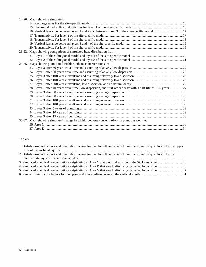
23-35. Maps showing simulated trichloroethene concentrations in:23. Layer 3 after 60 years traveltime and assuming relatively low dispersion............................................................2224. Layer 1 after 60 years traveltime and assuming relatively low dispersion............................................................2325. Layer 3 after 100 years traveltime and assuming relatively low dispersion..........................................................2526. Layer 1 after 100 years traveltime and assuming relatively low dispersion..........................................................2527. Layer 1 after 200 years traveltime, low dispersion, and no natural decay.............................................................2628. Layer 1 after 40 years traveltime, low dispersion, and first-order decay with a half-life of 13.5 years ................2729. Layer 3 after 60 years traveltime and assuming average dispersion......................................................................2930. Layer 1 after 60 years traveltime and assuming average dispersion......................................................................2931. Layer 3 after 100 years traveltime and assuming average dispersion....................................................................3032. Layer 1 after 100 years traveltime and assuming average dispersion....................................................................3033. Layer 3 after 5 years of pumping ...........................................................................................................................3234. Layer 3 after 10 years of pumping .........................................................................................................................3235. Layer 3 after 15 years of pumping .........................................................................................................................33
36-37. Maps showing simulated change in trichloroethene concentrations in pumping wells at:36. Area C ....................................................................................................................................................................3337. Area D ....................................................................................................................................................................34
Tables
1. Distribution coefficients and retardation factors for trichloroethene, cis-dichloroethene, and vinyl chloride for the upper layer of the surficial aquifer .................................................................................................................................................13
2. Distribution coefficients and retardation factors for trichloroethene, cis-dichloroethene, and vinyl chloride for the intermediate layer of the surficial aquifer ............................................................................................................................13
3. Simulated chemical concentrations originating at Area C that would discharge to the St. Johns River..............................234. Simulated chemical concentrations originating at Area D that would discharge to the St. Johns River .............................265. Simulated chemical concentrations originating at Area G that would discharge to the St. Johns River ............................ 276. Range of retardation factors for the upper and intermediate layers of the surficial aquifer.................................................31

Contents V
CONVERSION FACTORS
ABBREVIATIONS AND ACRONYMS
Degrees Celsius (°C) may be converted to degrees Fahrenheit (°F) by the following equation: °F = 9/5 (°C) + 32
Sea level: In this report, “sea level” refers to the National Geodetic Vertical Datum of 1929 (NGVD of 1929)—a geodetic datum derived from a general adjustment of the first-order level nets of the United States and Canada, formerly called Sea Level Datum of 1929.
Multiply By To obtain
inch (in.) 2.54 centimeter
foot (ft) 0.3048 meter
acre 0.4047 hectare
foot per year (ft/yr) 0.3048 meter per year
foot per day (ft/d) 0.3048 meter per year
foot squared per day (ft2/d) 0.09290 meter squared per day
gallon per minute (gal/min) 3.785 liter per minute
bsl below sea level
DCE cis-dichloroethene
cm3 cubic meter
HLA Harding Lawson Associates
g gram
g/g gram per gram
g/cm3 gram per cubic centimeter
HMOC Hybrid Method of Characteristics
kg kilogram
µg/L microgram per liter
mg milligram
mL milliliter
MOC Method of Characteristics
MMOC Modified Method of Characteristics
MODFLOW Modular Three-Dimensional Finite-DifferenceGround-Water Flow Model
MD3DMS Modular Three-Dimensional Multi-SpeciesTransport Model
OU3 Operable Unit 3
TCE trichloroethene
VC vinyl chloride
USEPA U.S. Environmental Protection Agency
USGS U.S. Geological Survey
Additional Abbreviations
Koc partition coefficient
Kd distribution coefficient
foc fraction organic carbon
mLwater/goc milliliter water per grams organic carbon
goc/gsoil grams organic carbon per grams soil
mgorganic carbon/kgsoil milligrams organic carbon per kilograms soil
mLwater/cm3soil milliliter water per cubic centimeters soil
mLwater/gsoil milliliter water per grams soil

VI Contents
Introduction 1
Fate and Transport Modeling of Selected Chlorinated Organic Compounds at Operable Unit 3, U.S. Naval Air Station, Jacksonville, Florida
By J. Hal Davis
Abstract
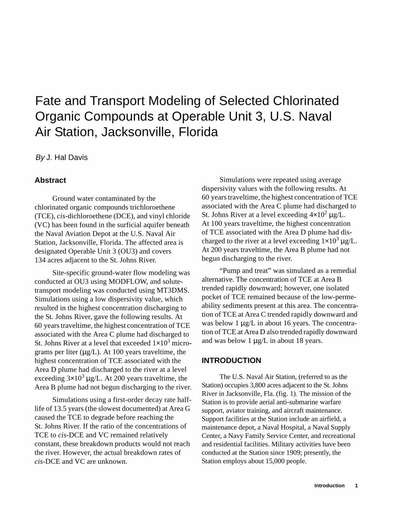
Ground water contaminated by the chlorinated organic compounds trichloroethene (TCE), cis-dichloroethene (DCE), and vinyl chloride (VC) has been found in the surficial aquifer beneath the Naval Aviation Depot at the U.S. Naval Air Station, Jacksonville, Florida. The affected area is designated Operable Unit 3 (OU3) and covers 134 acres adjacent to the St. Johns River.
Site-specific ground-water flow modeling was conducted at OU3 using MODFLOW, and solute-transport modeling was conducted using MT3DMS. Simulations using a low dispersivity value, which resulted in the highest concentration discharging to the St. Johns River, gave the following results. At 60 years traveltime, the highest concentration of TCE associated with the Area C plume had discharged to St. Johns River at a level that exceeded 1×10³ micro-grams per liter (µg/L). At 100 years traveltime, the highest concentration of TCE associated with the Area D plume had discharged to the river at a level exceeding 3×10³ µg/L. At 200 years traveltime, the Area B plume had not begun discharging to the river.
Simulations using a first-order decay rate half-life of 13.5 years (the slowest documented) at Area G caused the TCE to degrade before reaching the St. Johns River. If the ratio of the concentrations of TCE to cis-DCE and VC remained relatively constant, these breakdown products would not reach the river. However, the actual breakdown rates of cis-DCE and VC are unknown.
Simulations were repeated using average dispersivity values with the following results. At 60 years traveltime, the highest concentration of TCE associated with the Area C plume had discharged to St. Johns River at a level exceeding 4×10² µg/L. At 100 years traveltime, the highest concentration of TCE associated with the Area D plume had dis-charged to the river at a level exceeding 1×10³ µg/L. At 200 years traveltime, the Area B plume had not begun discharging to the river.
“Pump and treat” was simulated as a remedial alternative. The concentration of TCE at Area B trended rapidly downward; however, one isolated pocket of TCE remained because of the low-perme-ability sediments present at this area. The concentra-tion of TCE at Area C trended rapidly downward and was below 1 µg/L in about 16 years. The concentra-tion of TCE at Area D also trended rapidly downward and was below 1 µg/L in about 18 years.
INTRODUCTION
The U.S. Naval Air Station, (referred to as the Station) occupies 3,800 acres adjacent to the St. Johns River in Jacksonville, Fla. (fig. 1). The mission of the Station is to provide aerial anti-submarine warfare support, aviator training, and aircraft maintenance. Support facilities at the Station include an airfield, a maintenance depot, a Naval Hospital, a Naval Supply Center, a Navy Family Service Center, and recreational and residential facilities. Military activities have been conducted at the Station since 1909; presently, the Station employs about 15,000 people.

2 Fate and Transport Modeling of Selected Chlorinated Organic Compounds at Operable Unit 3, U.S. Naval Air Station, Jacksonville, Florida
DUVALCOUNTY
0 50 MILES
OPERABLE UNIT LOCATION AND NUMBER
EXPLANATION
OU1
St .
Jo
hn
sR
i ve
r
Ort
eg
aR
ive
r
NAVAL AIR STATION,JACKSONVILLE
17
17
OU2
OU3
OU130
30
81 81
0 0.5 1 MILE
Tim
uqua
naC
ount
ryC
lub
295
0 10 MILES
AT
LAN
TIC
OC
EA
N
30
30
82 8145
Nassau River
DUVALCOUNTY
CLAY COUNTY
ST. JOHNSCOUNTY
NASSAUCOUNTY
BA
KE
RC
OU
NT
Y 10
95
295
10
90
A1A
JACKSONVILLE
Naval Air Station,Jacksonville
GE
OR
GIA
FLO
RID
A
95
St.
John
sR
iver
Figure 1. Location of the Jacksonville Naval Air Station.

Introduction 3
The Station was placed on the U.S. Environmen-tal Protection Agency’s (USEPA) National Priorities List in December 1989, and is participating in the U.S. Department of Defense Installation Restoration Program, which serves to identify and remediate environmental contamination in compliance with the Comprehensive Environmental Response, Compensa-tion, and Liability Act and the Superfund Amendments and Reauthorization Act of 1980 and 1985, respec-tively. On October 23, 1990, the Station entered into a Federal Facility Agreement with the USEPA and the Florida Department of Environmental Protection, which designated Operable Units 1, 2, and 3 at the Station (U.S. Navy, 1994a). Operable Units were designated in areas where several sources of similar contamination existed in close proximity. The purpose was to allow the contaminated areas to be addressed in one coordinated effort. Operable Unit 1 was the Station landfill; this site has been discussed in previous studies (Davis and oth-ers, 1996). Operable Unit 2 was the wastewater treat-ment plant, which has been remediated; this site had minimal ground-water contamination. Operable Unit 3 (OU3) is the subject of this report.
OU3 occupies 134 acres on the eastern side of the Station (fig. 1). The area encompassed by OU3 is currently used for industrial and commercial purposes. The principal tenant is the Naval Aviation Depot, where approximately 3,000 personnel are employed in servic-ing and refurbishing numerous types of military aircraft. Waste materials spilled or disposed of at OU3 include paint sludges, solvents, battery acids, aviation fuels, petroleum lubricants, and radioactive materials (U.S. Navy, 1994a). The chlorinated organic compounds trichloroethene (TCE), cis-dichloroethene (cis-DCE), and vinyl chloride (VC) have been detected in the ground water of the surficial aquifer underlying OU3 (U.S. Navy, 1994a). Current investigations indicate that ground-water contamination is restricted to nine isolated “hot spot” areas. In six of these areas, chlorinated organic compounds are present only in the upper layer of the surficial aquifer; in the other three, the compounds are present only in the intermediate layer.
The Navy documented the occurrence and distri-bution of contamination at OU3 through the contractor, Harding Lawson Associates (HLA). Currently, HLA is determining if the contamination poses risks to human health or the environment. In support of this effort, the U.S. Geological Survey (USGS) conducted a ground-water flow and contaminant transport model, which is the subject of this report.
Hydrologic Setting
The climate for Jacksonville is humid subtropical, with an average annual rainfall and temperature for 1967-96 of 60.63 inches and 78 °F, respectively. Most of the annual rainfall occurs in late spring and early summer (Fairchild, 1972). Rainfall distribution is highly variable because most comes from scattered convective thunderstorms during the summer. Winters are mild and dry with occasional frost from November through February (Fairchild, 1972).
Land-surface topography consists of gently rolling hills, with elevations ranging from about 30 feet (ft) above sea level at hilltops to 1 ft above sea level at the shorelines of the St. Johns and Ortega Rivers. The Station is located in the Dinsmore Plain of the North-ern Coastal Strip of the Sea Island District in the Atlantic Coastal Plain Section (Brooks, 1981). The Dinsmore Plain is characterized by low-relief, clastic terrace deposits of Pleistocene to Holocene age (Brooks, 1981).
The surficial aquifer is exposed at land surface and forms the uppermost permeable unit at the Station. The aquifer is composed of sedimentary deposits of Pliocene to Holocene age (fig. 2), and consists of 30 to 100 ft of tan to yellow, medium to fine unconsolidated silty sands interbedded with lenses of clay, silty clay, and sandy clay (U.S. Navy, 1994a). The Pleistocene-age sedimentary deposits in Florida were deposited in a series of terraces formed during marine transgres-sions and regressions associated with glacial and inter-glacial periods (Miller, 1986).
The surficial aquifer is composed of two distinct layers at OU3 (fig. 3). The upper layer is unconfined and extends from land surface to about 10 to15 ft below sea level (bsl). Below the upper layer is the intermediate layer, which is confined and extends downward to the top of the Hawthorn Group. The upper and intermediate layers are separated in some areas by a low-permeability clay layer, ranging from 0- to 20-ft thick; clay exists in the northern and central parts of OU3.
The base of the surficial aquifer is formed by the Miocene-age Hawthorn Group, which is mainly composed of low-permeability clays (Scott, 1988). The top of the Hawthorn Group ranges from 35 to 100 ft bsl at the Station and is about 100 ft bsl at OU3. The Hawthorn Group is approximately 300-ft thick and composed of dark gray and olive-green sandy to silty clay, clayey sand, clay, and sandy limestone, all

4 Fate and Transport Modeling of Selected Chlorinated Organic Compounds at Operable Unit 3, U.S. Naval Air Station, Jacksonville, Florida
containing moderate to large amounts of black phosphatic sand, granules, or pebbles (Fairchild, 1972; Scott, 1988).
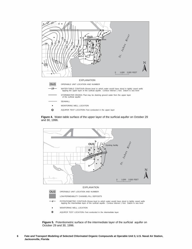
In the vicinity of OU3, the water table generally slopes eastward toward the St. Johns River (fig. 4). A seawall, which bounds OU3 along the eastern side, partially blocks ground-water flow in the upper layer along the central and northern edge of OU3. Ground-water flow is blocked where the seawall extends down-ward about 20 ft into the clay layer that separates the upper and intermediate layers. At the southern end of OU3, the seawall extends less than 20-ft deep and the clay layer is much less continuous. Lower heads in this area indicate that ground water is seeping under or through the seawall.
An extensive stormwater-drainage system is present at OU3 and the surrounding areas. Photo-graphic surveys documented that ground-water seeps into the drains through joints and cracks in the pipes. Visual inspection of the drains by Navy personnel indicated that the leakage is generally confined to high motor-traffic areas. Drain depths vary, but generally range from 5 to 10 ft bsl. Because the water level in the drains is below the water table, ground water
seeps from the aquifer into the drains; seepage from the drains to the aquifer seldom occurs. All drains are in the upper layer of the aquifer and have little or no effect on ground-water flow in the intermediate layer.
The potentiometric surface of the intermediate layer indicates that ground-water flow is generally eastward toward the St. Johns River (fig. 5). The east-ward movement of ground water is partially redirected by a naturally occurring, nearly vertical wall of low-permeability channel-fill deposits that crosses OU3 from west-southwest to north-northeast (figs. 3 and 5). These deposits extend from the top of the intermediate layer to or very near the bottom of the layer. U.S. Geological Survey topographic maps, made prior to construction at the Station, show that a deeply incised creek or inlet existed where the channel-fill deposits occur in the subsurface. These deposits could be the result of infilling of an erosional channel by low-permeablity sediments.
A docking facility (formerly used to offload fuel barges) at the northeastern corner of OU3 projects into the St. Johns River (fig. 5). A channel was dredged in the river bottom to allow barge access to the dock. Dredging probably removed most or all of the upper layer of the surficial aquifer and may have removed or disturbed part
SY
ST
EM
SE
RIE
S
QU
AT
ER
NA
RY
TE
RT
IAR
Y
MIO
CE
NE
PLI
OC
EN
EH
OLO
CE
NE
PL
EIS
TO
CE
NE
FORMATION
MODEL LAYERSHYDROGEOLOGIC
UNIT
Undifferentiatedterrace and
shallow marinedeposits
HawthornGroup
Surficial aquifer
Confining unit No-flowboundary
No-flowboundary
No-flowboundary
Layer 1
Layer 1(Upper layer)Layer 1
(Upper layer)
Layer 2(Clay layer)
Layer 2(Intermediate layer)
Layer 3(Intermediate layer)
Layer 4(Intermediate layer)
REGIONAL MODEL SUBREGIONAL MODEL SOLUTE TRANSPORTMODEL
Note A: The clay between layers 1 and 2 was simulated by a low vertical conductance.SURFICIAL AQUIFER
EXPLANATION
See Note
Figure 2. Geologic units, hydrogeologic units, and equivalent layers used in the computer models.

Introduction 5
of the underlying clay layer. The potentiometric contours near the dock appear relatively depressed, indicating that ground water could be discharging from the intermediate layer into the river in this area.
A low-permeability clay layer ranging 0- to 20-ft thick separates the upper and intermediate layers in the northern part of OU3, but is absent in the southern part (figs. 3 and 6). Ground-water flow in the upper and intermediate layers is effectively separated where the clay layer is present.
Previous Modeling at the Jacksonville Naval Air Station
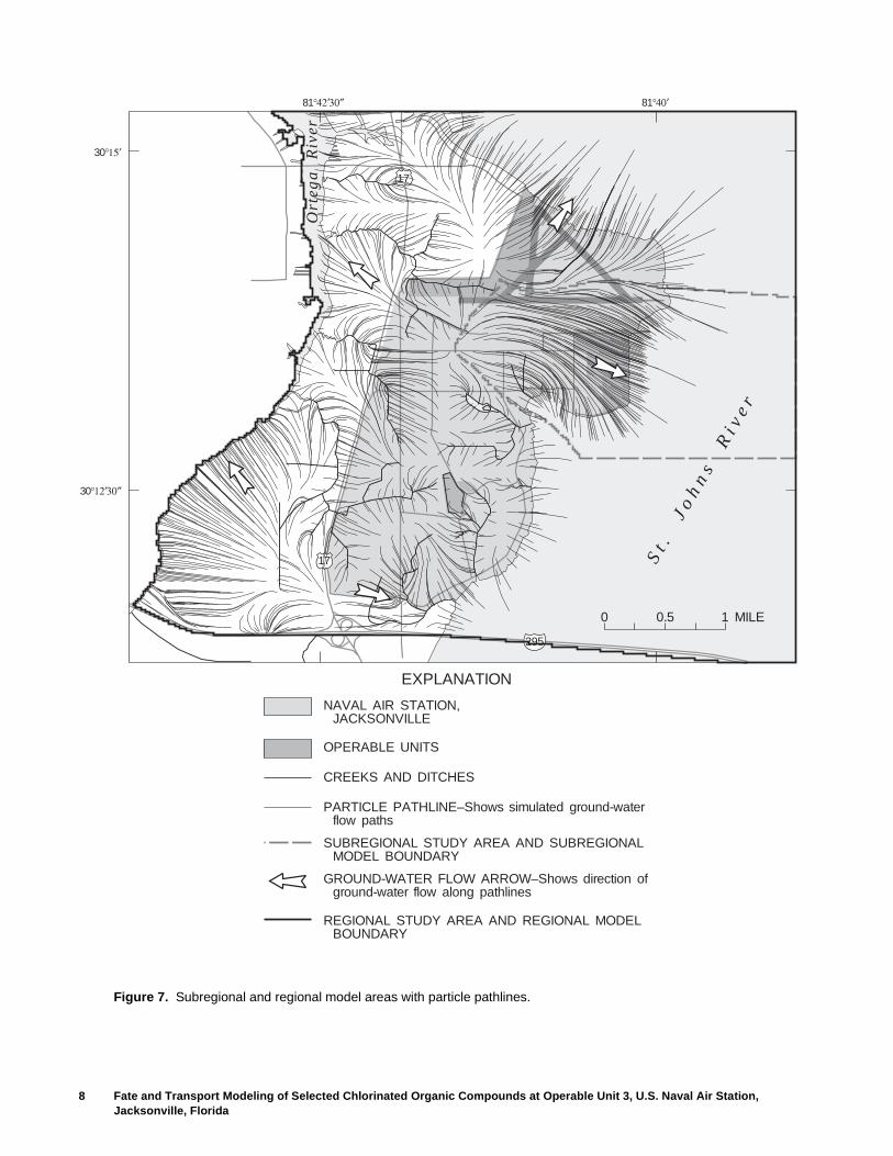
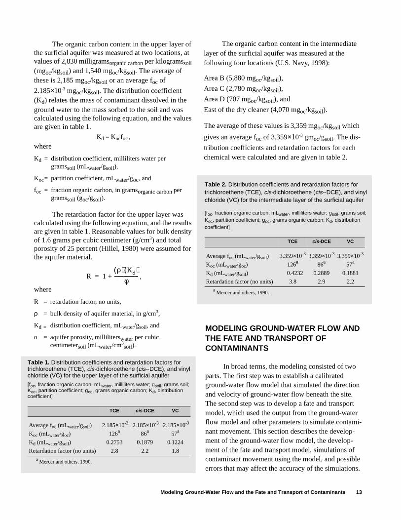
The USGS previously developed and calibrated a regional one-layer ground-water flow model that simulated steady-state flow in the surficial aquifer (Davis and others, 1996). The model used the USGS Modular Three-Dimensional Finite-Difference Ground-Water Flow Model (MODFLOW) as described in McDonald and Harbaugh (1988). The regional model had 240 rows and 290 columns with a uniform cell size of 100 by 100 ft, and simulated steady-state flow beneath the entire Station and some surrounding areas (fig. 7). The calibrated regional model matched the water levels to within 2.5 ft in 130 of 131 wells. The model was used to determine the direction and velocity of ground-water flow at Opera-ble Unit 1, as well as to evaluate the effect of proposed remediation scenarios on ground-water flow. This model was used to establish the boundary conditions for the subregional model discussed below.
A subregional ground-water flow model was developed to investigate ground-water flow at OU3. Documented by Davis (1998), this model simulated steady-state flow conditions (the relation between the regional and subregional model is shown in fig. 7). The model had 78 rows and 148 columns with a uniform cell size of 100 by 100 ft. The surficial aquifer was represented by two model layers to simulate the more complex hydrology present at and around OU3. Model layer 1 represented the upper layer of the surfi-cial aquifer and extended from land surface to 15 ft bsl; this layer was modeled as unconfined. Model layer 2 represented the intermediate layer and extended from the upper layer to the top of the Hawthorn Group; this layer was modeled as confined. The low-permeability clay separating layers 1 and 2 was not modeled explic-itly, but the effect of the clay layer was simulated through a low vertical leakance. After calibration, all model-simulated heads matched the measured heads within the calibration criterion of 1 ft, and 48 of 67 simulated heads (72 percent) were within 0.5 ft of the corresponding measured values. This model was used to establish the boundary conditions for a site-specific solute-transport model, which is the subject of this report.
30
20
10
10
20
30
40
50
60
70
80
90
SeaLevel
FEET
St.JohnsRiver
OU3
Vertical scale greatly exaggerated
0 1 MILE
A
Sea
wal
l
OU3
0 2,000 FEET
A A
A
St .
Jo
hn
sR
ive
r
Upper layer
ClayIntermediate layer
Hawthorn Group
Low
-per
mea
bilit
ych
anne
l-fill
depo
sits
SURFICIAL AQUIFER
OPERABLE UNIT 3–Location and number
EXPLANATION
OU3
Figure 3. Generalized hydrogeologic section through the subregional study area.
6 Fate and Transport Modeling of Selected Chlorinated Organic Compounds at Operable Unit 3, U.S. Naval Air Station, Jacksonville, Florida
St .
Jo
hn
sR
ive
r
OU3
0 1,000 2,000 FEET
17 1615
14
14
13
1312
1110 9 8
76 5
56
4
4
2
3
319
2021
18
EXPLANATION
WATER-TABLE CONTOUR–Shows level to which water would have stood in tightly cased wellstapping the upper layer of the surficial aquifer. Contour interval 1 foot. Datum is sea level
STORMWATER DRAINS–That may be draining ground water from the upper layerof the surficial aquifer
SEAWALL
MONITORING WELL LOCATION
AQUIFER TEST LOCATION–Test conducted in the upper layer
19
OPERABLE UNIT LOCATION AND NUMBEROU3
Figure 4. Water-table surface of the upper layer of the surficial aquifer on October 29 and 30, 1996.
OU3
EXPLANATION
Docking facility
6
4
6
3
35 4
0 1,000 2,000 FEET
St .
Jo
hn
sR
ive
r
POTENTIOMETRIC CONTOUR–Shows level to which water would have stood in tightly cased wellstapping the intermediate layer of the surficial aquifer. Contour interval 1 foot. Datum is sea level
LOW-PERMEABILITY CHANNEL-FILL DEPOSITS
MONITORING WELL LOCATION
AQUIFER TEST LOCATION–Test conducted in the intermediate layer
4
OPERABLE UNIT LOCATION AND NUMBEROU3
Figure 5. Potentiometric surface of the intermediate layer of the surficial aquifer on October 29 and 30, 1996.

Introduction 7
Purpose and Scope
The purpose of this study was to develop a computer model capable of simulating the fate and transport of TCE, cis-DCE, and VC in the ground water at OU3. The purpose of this report is to document the development of the model, describe application of the model to the study area, and provide the results of the model application. In order to apply this model to the study area, the occurrence of TCE and its degradation products were identified, factors affecting the movement and concentration of TCE and its degradation products were addressed, and site-specific ground-water flow modeling was conducted using MODFLOW. Model simulations
included the movement of plumes under current conditions and the recovery of contaminated ground water using pumping wells.
Acknowledgments
The author expresses appreciation to Dana Gaskins, Cliff Casey, and Anthony Robinson of U.S. Navy, Southern Division, Naval Facilities Engineer-ing Command; Diane Lancaster, Tim Curtis, and Christine Wolfman, of the Station; and Phylissa Miller, Willard Murray, Wayne Britton and Fred Bragdon of Harding Lawson Associates.
0 500 1,000 FEET
OU310
10
1020
20
15
15
155
5
9
6
6
8
10
15
15
0 0
02
2
20
20
20
20
20
St .
Jo
hn
sR
ive
r
EXPLANATION
2
LINE OF EQUAL THICKNESS OF CLAY THAT SEPARATES THEUPPER AND INTERMEDIATE LAYERS–Contour interval is 5 feet
WELL LOCATION–Number is thickness of clay, in feet
5
OPERABLE UNIT LOCATION AND NUMBEROU3
Figure 6. Thickness of the clay layer that separates the upper and intermediate layers of the surficial aquifer.
8 Fate and Transport Modeling of Selected Chlorinated Organic Compounds at Operable Unit 3, U.S. Naval Air Station, Jacksonville, Florida
St .
Jo
hn
sR
i ve
r
Ort
eg
aR
ive
r
295
30
30
81 81
0 0.5 1 MILE
EXPLANATION
CREEKS AND DITCHES
NAVAL AIR STATION,JACKSONVILLE
OPERABLE UNITS
PARTICLE PATHLINE–Shows simulated ground-waterflow paths
GROUND-WATER FLOW ARROW–Shows direction ofground-water flow along pathlines
SUBREGIONAL STUDY AREA AND SUBREGIONALMODEL BOUNDARY
REGIONAL STUDY AREA AND REGIONAL MODELBOUNDARY
17
17
Figure 7. Subregional and regional model areas with particle pathlines.

Background 9
0 500 1,000 FEET
EXPLANATION
34
33
16
17, 37
17, 37
1515
2220
unk
2010
42
3434
35
37
373734
38
35 353567
35
40
35unk
unk
unk
3132
35
OPERABLE UNIT LOCATION AND NUMBER
GROUND-WATER QUALITY SAMPLING LOCATION–Number is well depth orsampling point depth, in feet below land surface. unk indicates unknown depth.
22
OU3
St .
Jo
hn
sR
ive
r
OU3
Figure 8. Location of wells and sampling points where ground-water quality samples were taken.
BACKGROUND
The ground-water contaminants of concern at OU3 are TCE, cis-DCE, and VC. The current locations of these chemicals in the ground water and the factors affecting their future movement is discussed in this section. Because the chemicals are at concentrations that could be dangerous to human health and the envi-ronment, HLA is evaluating the chemicals as part of the risk-assessment process. The extent of the contami-nant plumes described in this section is based on data collected by HLA and is more fully discussed in Navy documentation (U.S. Navy, written commun., 1999). The location of sampling points used to define the plumes is shown in figure 8.
Occurrence of TCE, cis-DCE, and VC
TCE, cis-DCE, and VC are known to degrade in natural environments due to reductive dehalogenation. TCE degrades to cis-DCE that, in turn, degrades to VC, which can further degrade to ethene. Degradation occurs when a chlorine molecule is removed and replaced by a hydrogen molecule. The rate of
degradation can be extremely variable even over small distances, depending on the particular compound and the microenvironments within the aquifer.
The distribution of TCE in ground water is shown in figure 9. There are five major areas of elevated TCE concentrations: B, C, D, G, and H. The TCE at Areas B, C, and D is in the intermediate layer of the aquifer and, thus, below the clay that separates this layer from the upper layer. The Station’s dry cleaner is probably the source of TCE contamination at Area D because the dry cleaner is directly upgradient. The dry cleaning facility was built in 1962, and chlori-nated organic compounds were later documented in the upper layer of the aquifer beneath the dry cleaner (U.S. Navy, 1994b). Presently, no TCE contamination occurs in the relatively clean sediments underlying the still-active dry cleaner, so the plume is no longer considered to exist in that area and the dry cleaner is not consid-ered to be an ongoing source of contamination. The source of TCE contamination at Areas B and C is unknown. The TCE at Area G occurs mainly in the upper layer of the aquifer and is the result of waste disposal of solvents and paints (U.S. Navy, 1994a).

10 Fate and Transport Modeling of Selected Chlorinated Organic Compounds at Operable Unit 3, U.S. Naval Air Station, Jacksonville, Florida
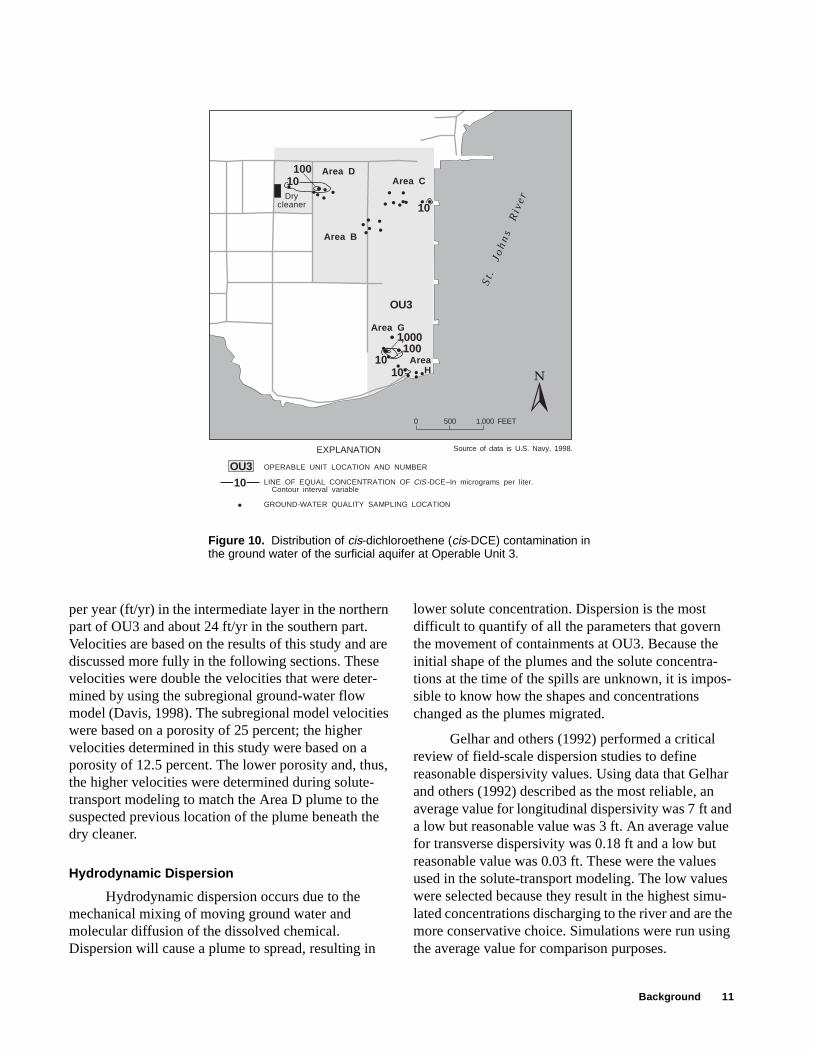
The distribution of cis-DCE in ground water is shown in figure 10. The source of cis-DCE contamina-tion is probably the result of reductive dehalogenation of TCE. Concentrations of cis-DCE at Areas C and D are relatively low compared to concentrations of TCE at the same areas, indicating that the reductive dehalogenation is occurring relatively slowly. Concen-trations of TCE and cis-DCE at Area G are roughly equivalent, indicating that dehalogenation of TCE to cis-DCE is occurring faster at Area G than at Areas C and D.
The distribution of VC in ground water is shown in figure 11. Concentrations of VC are very low to nonexistent at Areas B, C, and D, indicating that the dehalogenation of cis-DCE to VC is occurring rela-tively slowly (or at least relatively slowly compared to the dehalogenation of VC to ethene). Concentrations of VC at Area G are relatively high, indicating that the dehalogenation of cis-DCE to VC is occurring relatively quickly.
Factors Affecting the Movement and Concen-tration of TCE, cis-DCE, and VC Plumes
Contaminant plumes are dissolved in ground water and will move in the direction of flow. However, other natural processes can modify the movement of plumes, causing contaminant concentrations to change or causing contaminants to move at different rates than the ground water. The major processes affecting plume movement are advection, hydrodynamic dispersion, chemical degradation, and retardation. Each of these is discussed separately.
Advection
The most important factor affecting plume movement is advection, which is the transport of dissolved constituents with the velocity and direction of ground-water flow. Ground water (containing the plumes) at OU3 discharges to the St. Johns River. Thus, the plumes will move in that direction. Ground-water flow velocity is estimated to be about 70 feet
0 500 1,000 FEET
EXPLANATION
OPERABLE UNIT LOCATION AND NUMBER
LINE OF EQUAL CONCENTRATION OF TCE–In micrograms per liter.Contour interval variable
GROUND-WATER QUALITY SAMPLING LOCATION
10
100
1001,000
100
1,000
10
10
1,000
1,000
10 100
10
OU3
10
Area D Area C
AreaB
Area G
AreaH
Drycleaner
Source of data is U.S. Navy, 1998.
St .
Jo
hn
sR
ive
r
OU3
Figure 9. Distribution of trichloroethene (TCE) contamination in the ground water of the surficial aquifer at Operable Unit 3.
Background 11
per year (ft/yr) in the intermediate layer in the northern part of OU3 and about 24 ft/yr in the southern part. Velocities are based on the results of this study and are discussed more fully in the following sections. These velocities were double the velocities that were deter-mined by using the subregional ground-water flow model (Davis, 1998). The subregional model velocities were based on a porosity of 25 percent; the higher velocities determined in this study were based on a porosity of 12.5 percent. The lower porosity and, thus, the higher velocities were determined during solute-transport modeling to match the Area D plume to the suspected previous location of the plume beneath the dry cleaner.
Hydrodynamic Dispersion
Hydrodynamic dispersion occurs due to the mechanical mixing of moving ground water and molecular diffusion of the dissolved chemical. Dispersion will cause a plume to spread, resulting in
lower solute concentration. Dispersion is the most difficult to quantify of all the parameters that govern the movement of containments at OU3. Because the initial shape of the plumes and the solute concentra-tions at the time of the spills are unknown, it is impos-sible to know how the shapes and concentrations changed as the plumes migrated.
Gelhar and others (1992) performed a critical review of field-scale dispersion studies to define reasonable dispersivity values. Using data that Gelhar and others (1992) described as the most reliable, an average value for longitudinal dispersivity was 7 ft and a low but reasonable value was 3 ft. An average value for transverse dispersivity was 0.18 ft and a low but reasonable value was 0.03 ft. These were the values used in the solute-transport modeling. The low values were selected because they result in the highest simu-lated concentrations discharging to the river and are the more conservative choice. Simulations were run using the average value for comparison purposes.
0 500 1,000 FEET
OU3
1001,000
10100
1010
10
EXPLANATION
OPERABLE UNIT LOCATION AND NUMBER
LINE OF EQUAL CONCENTRATION OF DCE–In micrograms per liter.Contour interval variable
GROUND-WATER QUALITY SAMPLING LOCATION
CIS-10
Area D
Area B
Area C
Area G
AreaH
Drycleaner
Source of data is U.S. Navy, 1998.
St .
Jo
hn
sR
ive
r
OU3
Figure 10. Distribution of cis-dichloroethene (cis-DCE) contamination in the ground water of the surficial aquifer at Operable Unit 3.

12 Fate and Transport Modeling of Selected Chlorinated Organic Compounds at Operable Unit 3, U.S. Naval Air Station, Jacksonville, Florida
Chemical Degradation of Contaminants
The rate of chemical degradation of contami-nants at Areas B, C, and D seems to be slow and the velocity of ground water is relatively fast. Conse-quently, contaminated ground water is expected to reach the St. Johns River before complete degradation occurs. As discussed previously, the source of TCE contamination at Area D is suspected to be the old dry cleaner because the facility is directly upgradient of the plume. The ultimate discharge point for this plume is the St. Johns River, about 3,000 ft from the dry cleaner. The leading edge of the TCE plume has already moved one-third of the total distance and is still at a concentration of several thousand micrograms per liter. The plume is expected to reach the river in concentrations exceeding regulatory limits. The source of the TCE at Areas B and C is unknown; the initial concentrations are unknown; thus, the rate of degradation is difficult to estimate directly. However, because these plumes are in the same vertical horizon of the aquifer as the plume at Area D, the degradation rate is assumed to be similar.
The rate of degradation at Area G seems to be relatively fast. A substantial reduction in TCE concentra-tions occurred at Area G in 1983, 1985, and 1996 (U.S. Navy, 1998). The estimated half-life for TCE at these areas ranged from 3.75 to 13.5 years (U.S. Navy, 1998).
Retardation
The rate of movement of a dissolved chemical depends on the ground-water flow velocity and the retardation factor of the particular chemical. The retardation factor is the ratio of the velocity of ground water to the velocity of the chemical. For example, a retardation factor of 1.5 means that ground water moves 1.5 times faster than the dissolved chemical. Retardation of TCE, cis-DCE, and VC occurs because these chemicals are nonpolar and this causes them to partition to the organic matter in the soil. Partitioning is a reversible process; molecules that have partitioned to the organic matter will move back into the ground water as relative concentrations change. Retardation and, therefore, retardation factors are a function of the fraction organic carbon content (foc) of the aquifer.
0 500 1,000 FEET
OU3
1001010
EXPLANATION
OPERABLE UNIT LOCATION AND NUMBER
LINE OF EQUAL CONCENTRATION OF VINYL CHLORIDE–In micrograms per liter
GROUND-WATER QUALITY SAMPLING LOCATION
10
Area G
Area D
Area B
Area C
AreaH
St .
Jo
hn
sR
ive
r
OU3
Figure 11. Distribution of vinyl chloride (VC) contamination in the ground water of the surficial aquifer at Operable Unit 3 .
Modeling Ground-Water Flow and the Fate and Transport of Contaminants 13
The organic carbon content in the upper layer of the surficial aquifer was measured at two locations, at values of 2,830 milligramsorganic carbon per kilogramssoil
(mgoc/kgsoil) and 1,540 mgoc/kgsoil. The average of these is 2,185 mgoc/kgsoil or an average foc of
2.185×10⁻³ mgoc/kgsoil. The distribution coefficient (Kd) relates the mass of contaminant dissolved in the ground water to the mass sorbed to the soil and was calculated using the following equation, and the values are given in table 1.
Kd = Kocfoc ,
where
The retardation factor for the upper layer was calculated using the following equation, and the results are given in table 1. Reasonable values for bulk density of 1.6 grams per cubic centimeter (g/cm3) and total porosity of 25 percent (Hillel, 1980) were assumed for the aquifer material.
,
where
Kd = distribution coefficient, milliliters water per gramssoil (mLwater/gsoil),
Koc= partition coefficient, mLwater/goc, and
foc = fraction organic carbon, in gramsorganic carbon per gramssoil (goc/gsoil).
R = retardation factor, no units,
ρ = bulk density of aquifer material, in g/cm3,
Kd = distribution coefficient, mLwater/gsoil, and
o = aquifer porosity, milliliterswater per cubic centimetersoil (mLwater/cm3
soil).
R 1ρ( ) Kd( )
φ--------------------+=
The organic carbon content in the intermediate layer of the surficial aquifer was measured at the following four locations (U.S. Navy, 1998):
Area B (5,880 mgoc/kgsoil),
Area C (2,780 mgoc/kgsoil),
Area D (707 mgoc/kgsoil), and
East of the dry cleaner (4,070 mgoc/kgsoil).
The average of these values is 3,359 mgoc/kgsoil which
gives an average foc of 3.359×10⁻³ gmoc/gsoil. The dis-
tribution coefficients and retardation factors for each chemical were calculated and are given in table 2.
MODELING GROUND-WATER FLOW AND THE FATE AND TRANSPORT OF CONTAMINANTS
In broad terms, the modeling consisted of two parts. The first step was to establish a calibrated ground-water flow model that simulated the direction and velocity of ground-water flow beneath the site. The second step was to develop a fate and transport model, which used the output from the ground-water flow model and other parameters to simulate contami-nant movement. This section describes the develop-ment of the ground-water flow model, the develop-ment of the fate and transport model, simulations of contaminant movement using the model, and possible errors that may affect the accuracy of the simulations.
Table 1. Distribution coefficients and retardation factors for trichloroethene (TCE), cis-dichloroethene (cis--DCE), and vinyl chloride (VC) for the upper layer of the surficial aquifer
[foc, fraction organic carbon; mLwater, milliliters water; gsoil, grams soil; Koc, partition coefficient; goc, grams organic carbon; Kd, distribution coefficient]
TCE cis-DCE VC
Average foc (mLwater/gsoil) 2.185×10⁻³ 2.185×10⁻³ 2.185×10⁻³
Koc (mLwater/goc) 126a 86a 57a
Kd (mLwater/gsoil) 0.2753 0.1879 0.1224
Retardation factor (no units) 2.8 2.2 1.8a Mercer and others, 1990.
Table 2. Distribution coefficients and retardation factors for trichloroethene (TCE), cis-dichloroethene (cis--DCE), and vinyl chloride (VC) for the intermediate layer of the surficial aquifer
[foc, fraction organic carbon; mLwater, milliliters water; gsoil, grams soil; Koc, partition coefficient; goc, grams organic carbon; Kd, distribution coefficient]
TCE cis-DCE VC
Average foc (mLwater/gsoil) 3.359×10⁻³ 3.359×10⁻³ 3.359×10⁻³
Koc (mLwater/goc) 126a 86a 57a
Kd (mLwater/gsoil) 0.4232 0.2889 0.1881
Retardation factor (no units) 3.8 2.9 2.2a Mercer and others, 1990.
14 Fate and Transport Modeling of Selected Chlorinated Organic Compounds at Operable Unit 3, U.S. Naval Air Station, Jacksonville, Florida
Ground-Water Flow Modeling
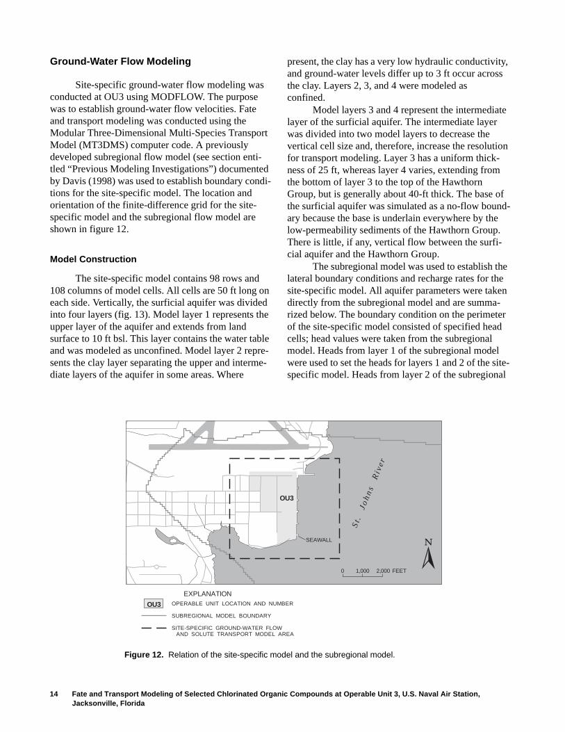
Site-specific ground-water flow modeling was conducted at OU3 using MODFLOW. The purpose was to establish ground-water flow velocities. Fate and transport modeling was conducted using the Modular Three-Dimensional Multi-Species Transport Model (MT3DMS) computer code. A previously developed subregional flow model (see section enti-tled “Previous Modeling Investigations”) documented by Davis (1998) was used to establish boundary condi-tions for the site-specific model. The location and orientation of the finite-difference grid for the site-specific model and the subregional flow model are shown in figure 12.
Model Construction
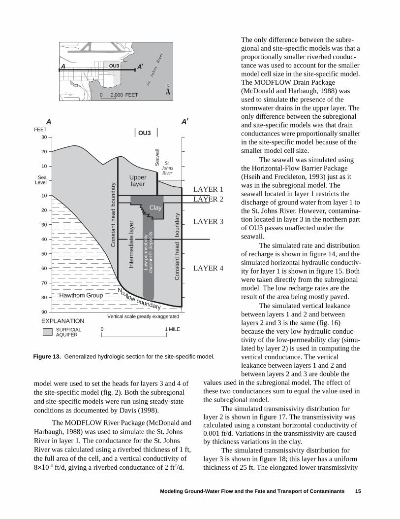
The site-specific model contains 98 rows and 108 columns of model cells. All cells are 50 ft long on each side. Vertically, the surficial aquifer was divided into four layers (fig. 13). Model layer 1 represents the upper layer of the aquifer and extends from land surface to 10 ft bsl. This layer contains the water table and was modeled as unconfined. Model layer 2 repre-sents the clay layer separating the upper and interme-diate layers of the aquifer in some areas. Where
present, the clay has a very low hydraulic conductivity, and ground-water levels differ up to 3 ft occur across the clay. Layers 2, 3, and 4 were modeled as confined.
Model layers 3 and 4 represent the intermediate layer of the surficial aquifer. The intermediate layer was divided into two model layers to decrease the vertical cell size and, therefore, increase the resolution for transport modeling. Layer 3 has a uniform thick-ness of 25 ft, whereas layer 4 varies, extending from the bottom of layer 3 to the top of the Hawthorn Group, but is generally about 40-ft thick. The base of the surficial aquifer was simulated as a no-flow bound-ary because the base is underlain everywhere by the low-permeability sediments of the Hawthorn Group. There is little, if any, vertical flow between the surfi-cial aquifer and the Hawthorn Group.
The subregional model was used to establish the lateral boundary conditions and recharge rates for the site-specific model. All aquifer parameters were taken directly from the subregional model and are summa-rized below. The boundary condition on the perimeter of the site-specific model consisted of specified head cells; head values were taken from the subregional model. Heads from layer 1 of the subregional model were used to set the heads for layers 1 and 2 of the site-specific model. Heads from layer 2 of the subregional
EXPLANATIONOPERABLE UNIT LOCATION AND NUMBER
SUBREGIONAL MODEL BOUNDARY
SITE-SPECIFIC GROUND-WATER FLOWAND SOLUTE TRANSPORT MODEL AREA
0 1,000 2,000 FEET
SEAWALL
OU3
St .
Jo
hn
sR
ive
r
OU3
Figure 12. Relation of the site-specific model and the subregional model.
Modeling Ground-Water Flow and the Fate and Transport of Contaminants 15
model were used to set the heads for layers 3 and 4 of the site-specific model (fig. 2). Both the subregional and site-specific models were run using steady-state conditions as documented by Davis (1998).
The MODFLOW River Package (McDonald and Harbaugh, 1988) was used to simulate the St. Johns River in layer 1. The conductance for the St. Johns River was calculated using a riverbed thickness of 1 ft, the full area of the cell, and a vertical conductivity of 8×10⁻⁴ ft/d, giving a riverbed conductance of 2 ft2/d.
The only difference between the subre-gional and site-specific models was that a proportionally smaller riverbed conduc-tance was used to account for the smaller model cell size in the site-specific model. The MODFLOW Drain Package (McDonald and Harbaugh, 1988) was used to simulate the presence of the stormwater drains in the upper layer. The only difference between the subregional and site-specific models was that drain conductances were proportionally smaller in the site-specific model because of the smaller model cell size.
The seawall was simulated using the Horizontal-Flow Barrier Package (Hseih and Freckleton, 1993) just as it was in the subregional model. The seawall located in layer 1 restricts the discharge of ground water from layer 1 to the St. Johns River. However, contamina-tion located in layer 3 in the northern part of OU3 passes unaffected under the seawall.
The simulated rate and distribution of recharge is shown in figure 14, and the simulated horizontal hydraulic conductiv-ity for layer 1 is shown in figure 15. Both were taken directly from the subregional model. The low recharge rates are the result of the area being mostly paved.
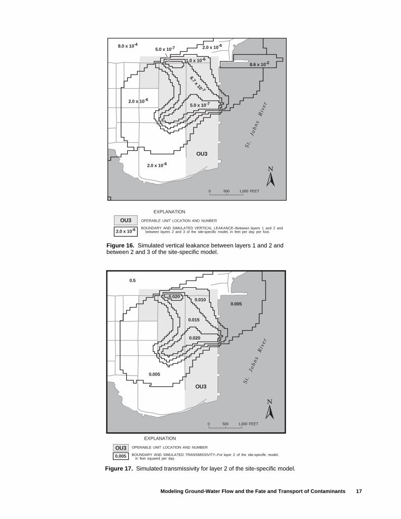
The simulated vertical leakance between layers 1 and 2 and between layers 2 and 3 is the same (fig. 16) because the very low hydraulic conduc-tivity of the low-permeability clay (simu-lated by layer 2) is used in computing the vertical conductance. The vertical leakance between layers 1 and 2 and between layers 2 and 3 are double the
values used in the subregional model. The effect of these two conductances sum to equal the value used in the subregional model.
The simulated transmissivity distribution for layer 2 is shown in figure 17. The transmissivity was calculated using a constant horizontal conductivity of 0.001 ft/d. Variations in the transmissivity are caused by thickness variations in the clay.
The simulated transmissivity distribution for layer 3 is shown in figure 18; this layer has a uniform thickness of 25 ft. The elongated lower transmissivity
30
20
10
10
20
30
40
50
60
70
80
90
SeaLevel
FEET
St.JohnsRiver
OU3
Vertical scale greatly exaggerated
0 1 MILE
A
Sea
wal
l
OU3
0 2,000 FEET
A A
A
St .
Jo
hn
sR
ive
r
LAYER 1
LAYER 3
LAYER 4
LAYER 2Clay
Hawthorn Group
SURFICIALAQUIFER
EXPLANATION
Con
stan
the
adbo
unda
ry
Upperlayer
No-flow bounda yr
Low
-per
mea
bilit
ych
anne
l-fill
depo
sits
Inte
rmed
iate
laye
r
Con
stan
the
adbo
unda
ry
Figure 13. Generalized hydrologic section for the site-specific model.

16 Fate and Transport Modeling of Selected Chlorinated Organic Compounds at Operable Unit 3, U.S. Naval Air Station, Jacksonville, Florida
0 500 1,000 FEET
OU3 St .
Jo
hn
sR
ive
r
EXPLANATION
OPERABLE UNIT LOCATION AND NUMBER
BOUNDARY AND SIMULATED HORIZONTAL HYDRAULIC CONDUCTIVITIES–Forlayer 1 of the solute transport model, in feet per day.1.000
0.500
1.000
OU3
Figure 15. Simulated horizontal hydraulic conductivities for layer 1 of the site-specific model.
0 500 1,000 FEET
St .
Jo
hn
sR
ive
r
OU3
EXPLANATION
OPERABLE UNIT LOCATION AND NUMBER
BOUNDARY AND SIMULATED RECHARGE RATES–For the solute transport model,in inches per year.1.000
0.400
1.000
0.000
OU3
Figure 14. Simulated recharge rates for the site-specific model.
Modeling Ground-Water Flow and the Fate and Transport of Contaminants 17
EXPLANATION
OPERABLE UNIT LOCATION AND NUMBER
BOUNDARY AND SIMULATED VERTICAL LEAKANCE–Between layers 1 and 2 andbetween layers 2 and 3 of the site-specific model, in feet per day per foot.2.0 x 10-6
0 500 1,000 FEET
OU3
2.0 x 10⁻⁶
2.0 x 10⁻⁶
2.0 x 10-68.0 x 10-45.0 x 10⁻⁷
1.0 x 10⁻⁶
5.0 x 10⁻⁷
8.6 x 10⁻²
6.7x 10 -7
St .
Jo
hn
sR
ive
r
OU3
Figure 16. Simulated vertical leakance between layers 1 and 2 and between 2 and 3 of the site-specific model.
0 500 1,000 FEET
St .
Jo
hn
sR
ive
r
OU3
OU3
EXPLANATION
OPERABLE UNIT LOCATION AND NUMBER
BOUNDARY AND SIMULATED TRANSMISSIVITY–For layer 2 of the site-specific model,in feet squared per day.
0.010
0.020
0.005
0.005
0.005
0.5
0.015
0.020
Figure 17. Simulated transmissivity for layer 2 of the site-specific model.

18 Fate and Transport Modeling of Selected Chlorinated Organic Compounds at Operable Unit 3, U.S. Naval Air Station, Jacksonville, Florida
0 500 1,000 FEET
OU3 St .
Jo
hn
sR
ive
r
10.0
500.0
OPERABLE UNIT LOCATION AND NUMBER
BOUNDARY AND SIMULATED TRANSMISSIVITY–For layer 3 of the site-specific model,in feet squared per day.
EXPLANATION
10.0
EXPLANATION
OU3
Figure 18. Simulated transmissivity for layer 3 of the site-specific model.
zone of 10 feet squared per day (ft2/d) corresponds to the lower permeability channel-fill deposits; the trans-missivity was calculated using a hydraulic conductivity of 0.4 ft/d. The transmissivity of the remaining part of layer 3 is 500 ft2/d which was calculated based on a hydraulic conductivity of 20 ft/d.
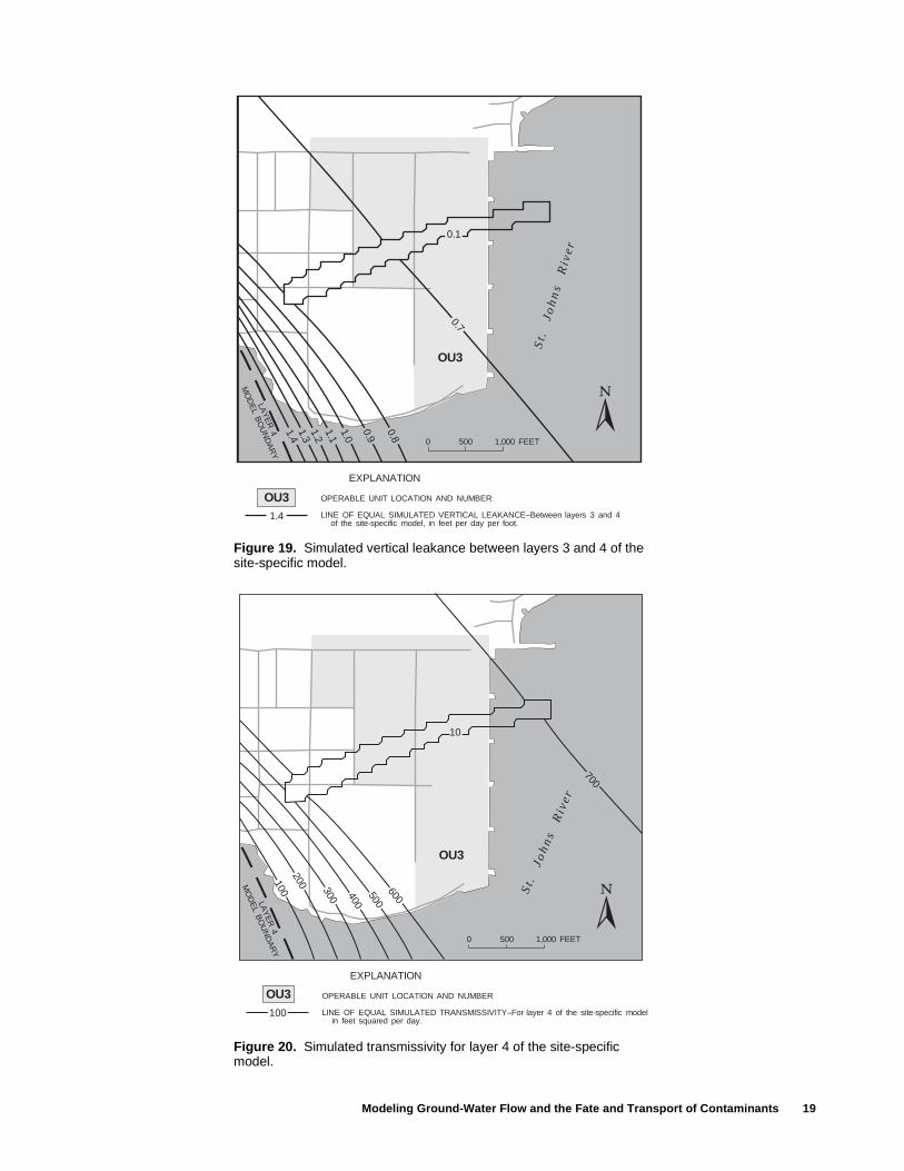
The simulated vertical leakance between layers 3 and 4 is shown in figure 19. The leakance was calcu-lated using a vertical hydraulic conductivity that was equal to the horizontal hydraulic conductivity. This calculation assured that ground-water flow properties of the site-specific model would be identical to the calibrated subregional model (combined layers 3 and 4 are identical to layer 2 of the subregional model). The simulated transmissivity distribution for layer 4 is shown in figure 20. As in layer 3, the elongated lower transmissivity zone of 10 ft2/d in layer 4 corresponds to the low-permeability channel-fill deposits; the transmissivity was calculated based on a hydraulic conductivity value of 0.4 ft/d. The transmissivity of the remaining part of layer 4 was calculated based on a hydraulic conductivity value of 20 ft/d. The variation in transmissivity is due to the variation in the thickness of layer 4.
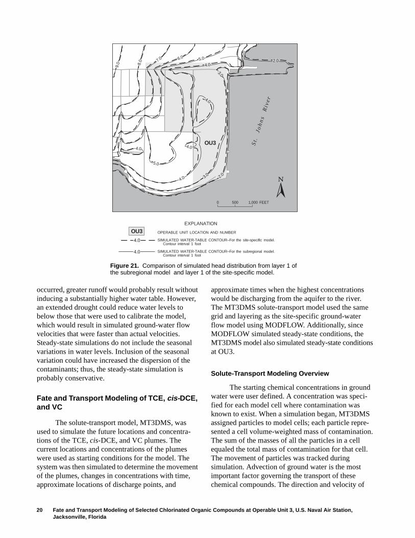
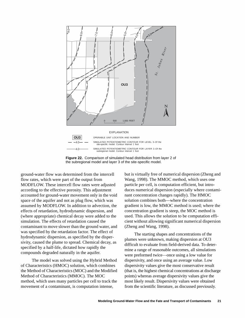
A comparison of the simulated water levels from layer 1 of the site-specific model and layer 1 of the subregional model is shown in figure 21. A compari-son of the simulated water levels from layer 3 of the site-specific model and layer 2 of the subregional model is shown in figure 22. The good agreement between the water levels shown in both of these figures indicates that the site-specific model is simulat-ing the aquifer in the same manner as the subregional model. Minor differences are probably due to the finer cell size and additional layering of the site-specific model. Additionally, the water balance between the site-specific model and the same area of the subre-gional model was equivalent.
Ground-Water Flow Model Limitations
The subregional model and the site-specific model are steady state. The surficial aquifer is under steady-state conditions because water levels in wells showed no long-term trend (but did show seasonal variation). The water table is generally close to the land surface, and there is little capacity for a substan-tial rise in water levels. If higher than average rainfall
Modeling Ground-Water Flow and the Fate and Transport of Contaminants 19
OPERABLE UNIT LOCATION AND NUMBER
LINE OF EQUAL SIMULATED TRANSMISSIVITY–For layer 4 of the site-specific modelin feet squared per day.
EXPLANATION
100
0 500 1,000 FEET
OU3
OU3
St .
Jo
hn
sR
ive
r
LAY
ER
4
MO
DE
LB
OU
ND
AR
Y
700
100200 300 400
600500
10
Figure 20. Simulated transmissivity for layer 4 of the site-specific model.
OPERABLE UNIT LOCATION AND NUMBER
LINE OF EQUAL SIMULATED VERTICAL LEAKANCE–Between layers 3 and 4of the site-specific model, in feet per day per foot.
EXPLANATION
1.4
St .
Jo
hn
sR
ive
r
OU3
OU3
0 500 1,000 FEET
1.31.21.11.0
0.9
1.4
0.8
0.7
0.1
LAY
ER
4
MO
DE
LB
OU
ND
AR
Y
Figure 19. Simulated vertical leakance between layers 3 and 4 of the site-specific model.
20 Fate and Transport Modeling of Selected Chlorinated Organic Compounds at Operable Unit 3, U.S. Naval Air Station, Jacksonville, Florida
occurred, greater runoff would probably result without inducing a substantially higher water table. However, an extended drought could reduce water levels to below those that were used to calibrate the model, which would result in simulated ground-water flow velocities that were faster than actual velocities. Steady-state simulations do not include the seasonal variations in water levels. Inclusion of the seasonal variation could have increased the dispersion of the contaminants; thus, the steady-state simulation is probably conservative.
Fate and Transport Modeling of TCE, cis-DCE, and VC
The solute-transport model, MT3DMS, was used to simulate the future locations and concentra-tions of the TCE, cis-DCE, and VC plumes. The current locations and concentrations of the plumes were used as starting conditions for the model. The system was then simulated to determine the movement of the plumes, changes in concentrations with time, approximate locations of discharge points, and
approximate times when the highest concentrations would be discharging from the aquifer to the river. The MT3DMS solute-transport model used the same grid and layering as the site-specific ground-water flow model using MODFLOW. Additionally, since MODFLOW simulated steady-state conditions, the MT3DMS model also simulated steady-state conditions at OU3.
Solute-Transport Modeling Overview
The starting chemical concentrations in ground water were user defined. A concentration was speci-fied for each model cell where contamination was known to exist. When a simulation began, MT3DMS assigned particles to model cells; each particle repre-sented a cell volume-weighted mass of contamination. The sum of the masses of all the particles in a cell equaled the total mass of contamination for that cell. The movement of particles was tracked during simulation. Advection of ground water is the most important factor governing the transport of these chemical compounds. The direction and velocity of
EXPLANATION
OPERABLE UNIT LOCATION AND NUMBER
SIMULATED WATER-TABLE CONTOUR–For the site-specific model.Contour interval 1 foot
SIMULATED WATER-TABLE CONTOUR–For the subregional model.Contour interval 1 foot
4.0
4.0
0 500 1,000 FEET
St .
Jo
hn
sR
ive
r
OU3
9.0 8.0 7.0 6.0 5.0
4.0
4.0
5.0
4.0
2.04.0
3.0
4.0
2.03.0
OU3
Figure 21. Comparison of simulated head distribution from layer 1 of the subregional model and layer 1 of the site-specific model.
Modeling Ground-Water Flow and the Fate and Transport of Contaminants 21
ground-water flow was determined from the intercell flow rates, which were part of the output from MODFLOW. These intercell flow rates were adjusted according to the effective porosity. This adjustment accounted for ground-water movement only in the void space of the aquifer and not as plug flow, which was assumed by MODFLOW. In addition to advection, the effects of retardation, hydrodynamic dispersion, and (where appropriate) chemical decay were added to the simulation. The effects of retardation caused the contaminant to move slower than the ground water, and was specified by the retardation factor. The effect of hydrodynamic dispersion, as specified by the disper-sivity, caused the plume to spread. Chemical decay, as specified by a half-life, dictated how rapidly the compounds degraded naturally in the aquifer.
The model was solved using the Hybrid Method of Characteristics (HMOC) solution, which combines the Method of Characteristics (MOC) and the Modified Method of Characteristics (MMOC). The MOC method, which uses many particles per cell to track the movement of a contaminant, is computation intense,
but is virtually free of numerical dispersion (Zheng and Wang, 1998). The MMOC method, which uses one particle per cell, is computation efficient, but intro-duces numerical dispersion (especially where contami-nant concentration changes rapidly). The HMOC solution combines both—where the concentration gradient is low, the MMOC method is used; where the concentration gradient is steep, the MOC method is used. This allows the solution to be computation effi-cient without allowing significant numerical dispersion (Zheng and Wang, 1998).
The starting shapes and concentrations of the plumes were unknown, making dispersion at OU3 difficult to evaluate from field-derived data. To deter-mine a range of reasonable outcomes, all simulations were preformed twice—once using a low value for dispersivity, and once using an average value. Low dispersivity values give the most conservative result (that is, the highest chemical concentrations at discharge points) whereas average dispersivity values give the most likely result. Dispersivity values were obtained from the scientific literature, as discussed previously.
St .
Jo
hn
sR
ive
r
OU3
OU3
0 500 1,000 FEET
EXPLANATION
OPERABLE UNIT LOCATION AND NUMBER
SIMULATED POTENTIOMETRIC CONTOUR FOR LEVEL 3–Of thesite-specific model. Contour interval 1 foot
SIMULATED POTENTIOMETRIC CONTOUR FOR LAYER 2–Of thesubregional model. Contour interval 1 foot
4.0
4.0
8.0
7.0
5.0
6.0
4.0
9.0
3.0
Figure 22. Comparison of simulated head distribution from layer 2 of the subregional model and layer 3 of the site-specific model.

22 Fate and Transport Modeling of Selected Chlorinated Organic Compounds at Operable Unit 3, U.S. Naval Air Station, Jacksonville, Florida
Determination of Effective Porosity
A reasonable effective porosity for the aquifer was established to simulate solute fate and transport. This was accomplished by modeling the movement of the leading edge of the TCE plume from the dry cleaner (established in 1962) to its present position at Area D. The plume was introduced as a single instantaneous pulse for this simulation. This is the only plume for which a reasonable starting date and location is known. The effective porosity was varied until the model simulation matched the known location. An effective porosity value of 12.5 percent gave the best match. This effective porosity was used in all subsequent fate and transport modeling. The effective porosity is different than the total aquifer porosity of 25 percent, which was used for the calculation of the retardation factors. The effective porosity represents only the part of the aquifer that is connected and readily allows for ground-water movement (such as the voids around the sand grains). The total aquifer poros-ity is composed of all the void spaces, including the very small, low-permeability voids between the fine silt and clay particles. Although the small voids do not add much to the overall permeability, the solute mole-cules can readily diffuse into them. For more discus-sion on this subject see Zheng and Bennett (1995).
The simulated concentrations reported herein were calculated by the model. However, there is a great deal of uncertainty in fate and transport model-ing. Simulation results can vary substantially with variations in the model input parameters, and the accuracy of the simulated future concentrations is unknown. Parameter effect on model simulation results are discussed the in a following section.
Modeling Results Assuming Low Dispersivity
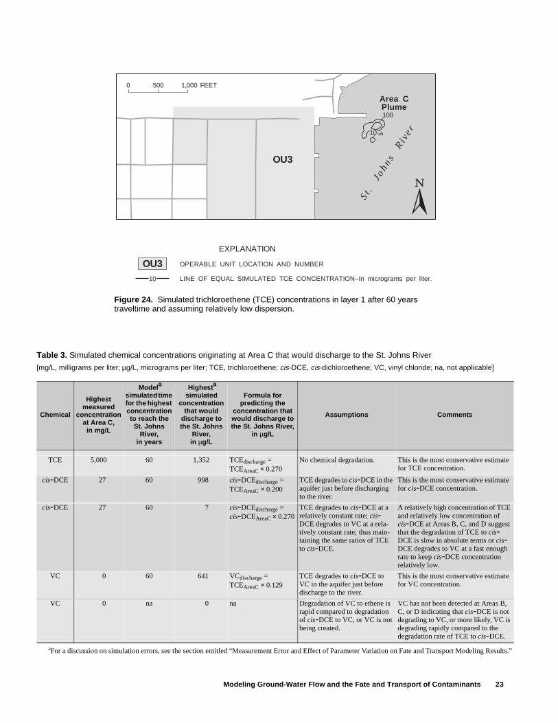
A horizontal dispersivity of 1 ft, a transverse dispersivity of 0.03 ft, and a vertical dispersivity of 0.03 ft were used in modeling the fate and transport of TCE. These values were at the low end of the expected range and, as discussed previously, resulted in the high-est, most conservative estimates of the discharge concentrations. The distribution of TCE in layers 3 and 1 for the Area B, C, and D plumes after 60 years traveltime is shown in figures 23 and 24, respectively. The Area B plume became elongated because it was in and near the low-permeability channel-fill deposits. The Area C plume moved completely beneath the river and began moving upward toward the river bottom. The Area D plume began moving under the river. The highest concentration of TCE discharging to the river, due to the Area C plume, occurred at 60 years traveltime and was simulated to be 1,352 micrograms per liter (µg/L) (table 3).
St .
Joh
ns
Riv
er
0 500 1,000 FEET
OU310
1010
100
100
1,000
1,000
1,00010
0
EXPLANATION
OPERABLE UNIT LOCATION AND NUMBER
LINE OF EQUAL SIMULATED TCE CONCENTRATION–In microgramsper liter. Interval is variable
10
Area D
Plume
Area CPlume
Area BPlume
OU3
Figure 23. Simulated trichloroethene (TCE) concentrations in layer 3 after 60 years traveltime and assuming relatively low dispersion.
Modeling Ground-Water Flow and the Fate and Transport of Contaminants 23
EXPLANATION
OPERABLE UNIT LOCATION AND NUMBER
LINE OF EQUAL SIMULATED TCE CONCENTRATION–In micrograms per liter.10
St .
Joh
ns
Riv
er
0 500 1,000 FEET
100
OU3
OU3
10
Area CPlume
Figure 24. Simulated trichloroethene (TCE) concentrations in layer 1 after 60 years traveltime and assuming relatively low dispersion.
Table 3. Simulated chemical concentrations originating at Area C that would discharge to the St. Johns River
[mg/L, milligrams per liter; µg/L, micrograms per liter; TCE, trichloroethene; cis-DCE, cis-dichloroethene; VC, vinyl chloride; na, not applicable]
Chemical
Highest measured
concentration at Area C,
in mg/L
Modela simulated time for the highest concentration to reach the
St. Johns River,
in years
Highesta simulated
concentration that would
discharge to the St. Johns
River,in µg/L
Formula for predicting the
concentration that would discharge to the St. Johns River,
in µg/L
Assumptions Comments
TCE 5,000 60 1,352 TCEdischarge =TCEAreaC × 0.270
No chemical degradation. This is the most conservative estimate for TCE concentration.
cis-DCE 27 60 998 cis-DCEdischarge =TCEAreaC × 0.200
TCE degrades to cis-DCE in the aquifer just before discharging to the river.
This is the most conservative estimate for cis-DCE concentration.
cis-DCE 27 60 7 cis-DCEdischarge =cis-DCEAreaC × 0.270
TCE degrades to cis-DCE at a relatively constant rate; cis-DCE degrades to VC at a rela-tively constant rate; thus main-taining the same ratios of TCE to cis-DCE.
A relatively high concentration of TCE and relatively low concentration of cis-DCE at Areas B, C, and D suggest that the degradation of TCE to cis-DCE is slow in absolute terms or cis-DCE degrades to VC at a fast enough rate to keep cis-DCE concentration relatively low.
VC 0 60 641 VCdischarge =TCEAreaC × 0.129
TCE degrades to cis-DCE to VC in the aquifer just before discharge to the river.
This is the most conservative estimate for VC concentration.
VC 0 na 0 na Degradation of VC to ethene is rapid compared to degradation of cis-DCE to VC, or VC is not being created.
VC has not been detected at Areas B, C, or D indicating that cis-DCE is not degrading to VC, or more likely, VC is degrading rapidly compared to the degradation rate of TCE to cis-DCE.
aFor a discussion on simulation errors, see the section entitled “Measurement Error and Effect of Parameter Variation on Fate and Transport Modeling Results.”

24 Fate and Transport Modeling of Selected Chlorinated Organic Compounds at Operable Unit 3, U.S. Naval Air Station, Jacksonville, Florida
After 100 years traveltime, the Area D plume had moved completely under the St. Johns River (figs. 25 and 26) and began moving vertically upward toward the river bottom. The highest concentration of TCE at this time, due to the Area D plume, was 3,434 µg/L. The Area C plume had largely migrated upward from layer 3 and the concentration was gener-ally less than 100 µg/L. The concentration in layer 1, due to the Area C plume, had dropped substantially due to upward leakage into the St. Johns River. The Area B plume had not yet begun to enter layer 1. The highest concentration in the Area B plume had migrated very little because this part of the plume was in lower permeability material.
Discussion of Area C Plume
The results of this study will be used by HLA to assess the risk of the dissolved chlorinated compounds to human health and the environment. The concentra-tion of these compounds must be predicted at the discharge point to the environment. The risk-assess-ment process involves selecting several representative wells from each area. The concentrations of contami-nants detected in the wells are then projected to the discharge point. The maximum concentration for TCE detected at Area C was 5,000 µg/L; the maximum simulated concentration discharging to the St. Johns River occurred after 60 years traveltime and was 1,352 µg/L. Using this ratio (1,352 µg/L divided by 5,000 µg/L = 0.270), the discharge concentration to the river for a concentration detected in an individual well can be estimated by using the following equation:
TCEdischarge = TCEAreaC × (0.270).
This procedure assumed no degradation of TCE.Using the equation, the most conservative
estimate of the discharge concentration for cis-DCE originating at Area C was made. This equation assumed that TCE was converted to cis-DCE just before discharging to the river. The 0.270 multiplier was used to estimate the concentration of TCE present at the discharge point and 0.739 (a cis-DCE molecule has 0.739 the mass of a TCE molecule) was used to correct for the mass change in the following equation:
cis-DCEdischarge = TCEAreaC × (0.270) × (0.739) =
TCEAreaC × (0.200).
This was the most conservative estimate for cis-DCE because the estimates assumed that all TCE degraded to cis-DCE immediately before discharging to the river. A more reasonable estimate of the cis-DCE concentration was made by assuming that
TCE degraded to cis-DCE at a relatively constant rate, that cis-DCE degraded to VC at a relatively constant rate and, thus, the same ratios of TCE to cis-DCE as are currently present at Area C were maintained. The cis-DCE discharge concentration can be estimated under these assumptions by using the formula:
cis-DCEdischarge = cis-DCEAreaC × (0.270).
Using the equation below, the most conservative estimate for the discharge concentration for VC was made by assuming that the TCE converted to cis-DCE, which then converted to VC just before discharging to the river. The 0.270 multiplier was used to estimate the concentration of TCE present at the discharge point and a 0.476 multiplier (a VC molecule has 0.476 the mass of a TCE molecule) was used to correct for the mass change.
VCdischarge = TCEAreaC × (0.270) × (0.476) =
TCEAreaC × (0.129).
VC had not been detected at Areas B, C, or D, indicating that either cis-DCE had not degraded to VC, or more likely, that VC had degraded rapidly to ethene (at least compared to the degradation rate of cis-DCE to VC). The discharge concentration of VC was 0. These equations and assumptions are summarized in table 3.
Discussion of Area D Plume
The maximum TCE concentration detected at Area D was 6,800 µg/L, and the maximum simulated concentration discharging to the St. Johns River was 3,434 µg/L at a traveltime of 100 years. The range of possible concentrations was determined for Area D by using the same methodology for computing discharge concentration as for Area C. The equations and assumptions are given in table 4.
Discussion of Area G Plume
The Area G plume location, after a traveltime of 200 years, is shown in figure 27. The ground-water velocities are substantially lower in this part of OU3, resulting in much slower migration. Natural degrada-tion of the chemicals has been documented at this area. When a first-order decay rate of 13.5 years was incor-porated into the model, the concentration of TCE dropped relatively quickly and the plume degraded before reaching the St. Johns River (fig. 28). The maximum concentration detected at Area G for TCE was 3,800 µg/L. The chemical concentrations that would discharge to the St. Johns River were simulated and are listed in table 5.
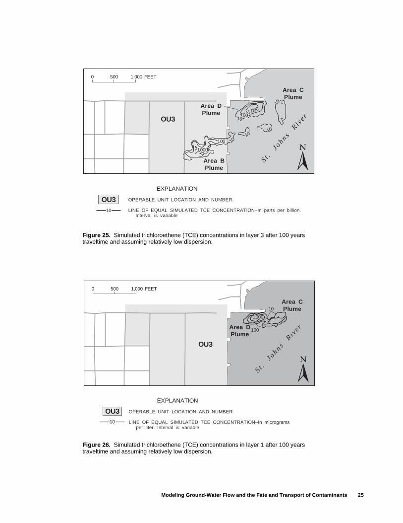
Modeling Ground-Water Flow and the Fate and Transport of Contaminants 25
EXPLANATION
OPERABLE UNIT LOCATION AND NUMBER
LINE OF EQUAL SIMULATED TCE CONCENTRATION–In microgramsper liter. Interval is variable
10
0 500 1,000 FEET
St .
JohnsR
iver
OU3
OU3
100
10
1,000
Area CPlume
Area DPlume
Figure 26. Simulated trichloroethene (TCE) concentrations in layer 1 after 100 years traveltime and assuming relatively low dispersion.
EXPLANATION
OPERABLE UNIT LOCATION AND NUMBER
LINE OF EQUAL SIMULATED TCE CONCENTRATION–In parts per billion.Interval is variable
10
St .
JohnsR
iver
0 500 1,000 FEET
OU3
OU3
1,000
100
1010
10
10
10
1,000
100
Area CPlume
Area DPlume
Area BPlume
Figure 25. Simulated trichloroethene (TCE) concentrations in layer 3 after 100 years traveltime and assuming relatively low dispersion.
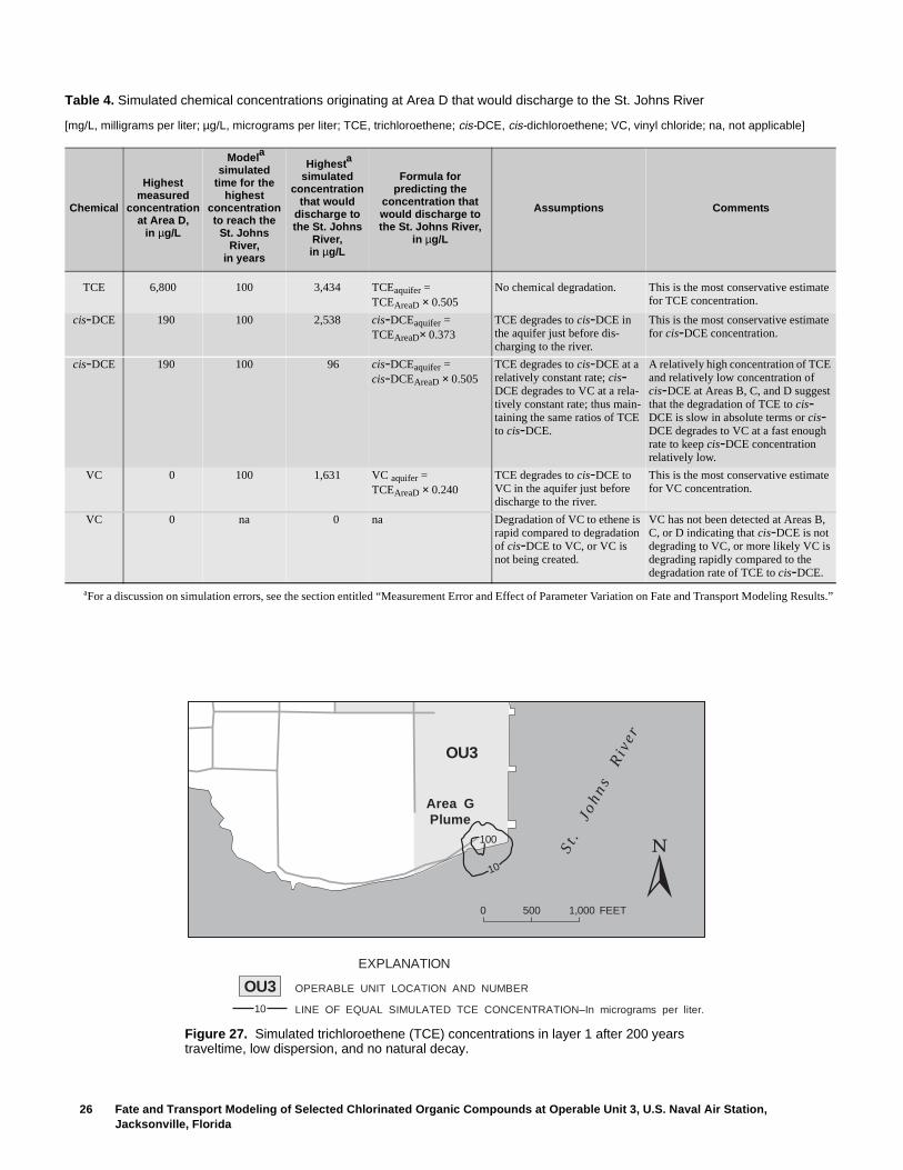
26 Fate and Transport Modeling of Selected Chlorinated Organic Compounds at Operable Unit 3, U.S. Naval Air Station, Jacksonville, Florida
Table 4. Simulated chemical concentrations originating at Area D that would discharge to the St. Johns River
[mg/L, milligrams per liter; µg/L, micrograms per liter; TCE, trichloroethene; cis-DCE, cis-dichloroethene; VC, vinyl chloride; na, not applicable]
Chemical
Highest measured
concentration at Area D,
in µg/L
Modela simulated
time for the highest
concentration to reach the
St. Johns River,
in years
Highesta simulated
concentration that would
discharge to the St. Johns
River,in µg/L
Formula for predicting the
concentration that would discharge to the St. Johns River,
in µg/L
Assumptions Comments
TCE 6,800 100 3,434 TCEaquifer =TCEAreaD × 0.505
No chemical degradation. This is the most conservative estimate for TCE concentration.
cis-DCE 190 100 2,538 cis-DCEaquifer =TCEAreaD× 0.373
TCE degrades to cis-DCE in the aquifer just before dis-charging to the river.
This is the most conservative estimate for cis-DCE concentration.
cis-DCE 190 100 96 cis-DCEaquifer =cis-DCEAreaD × 0.505
TCE degrades to cis-DCE at a relatively constant rate; cis-DCE degrades to VC at a rela-tively constant rate; thus main-taining the same ratios of TCE to cis-DCE.
A relatively high concentration of TCE and relatively low concentration of cis-DCE at Areas B, C, and D suggest that the degradation of TCE to cis-DCE is slow in absolute terms or cis-DCE degrades to VC at a fast enough rate to keep cis-DCE concentration relatively low.
VC 0 100 1,631 VC aquifer =TCEAreaD × 0.240
TCE degrades to cis-DCE to VC in the aquifer just before discharge to the river.
This is the most conservative estimate for VC concentration.
VC 0 na 0 na Degradation of VC to ethene is rapid compared to degradation of cis-DCE to VC, or VC is not being created.
VC has not been detected at Areas B, C, or D indicating that cis-DCE is not degrading to VC, or more likely VC is degrading rapidly compared to the degradation rate of TCE to cis-DCE.
aFor a discussion on simulation errors, see the section entitled “Measurement Error and Effect of Parameter Variation on Fate and Transport Modeling Results.”
0 500 1,000 FEET
St .
Joh
ns
Riv
er
OU3
OU3
10
100
EXPLANATION
OPERABLE UNIT LOCATION AND NUMBER
LINE OF EQUAL SIMULATED TCE CONCENTRATION–In micrograms per liter.10
Area GPlume
Figure 27. Simulated trichloroethene (TCE) concentrations in layer 1 after 200 years traveltime, low dispersion, and no natural decay.
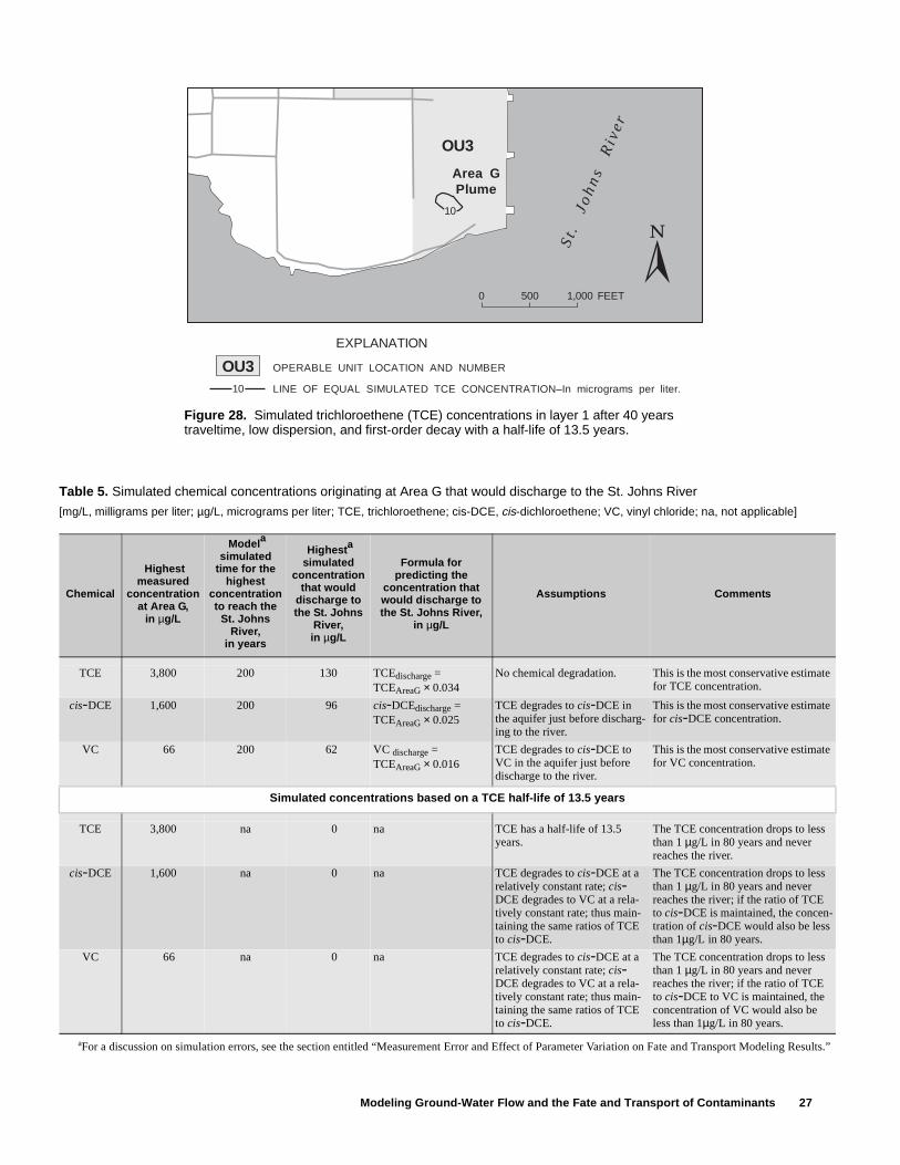
Modeling Ground-Water Flow and the Fate and Transport of Contaminants 27
0 500 1,000 FEET
St .
Jo
hn
sR
ive
r
OU3
EXPLANATION
OPERABLE UNIT LOCATION AND NUMBER
LINE OF EQUAL SIMULATED TCE CONCENTRATION–In micrograms per liter.10
OU3
10
Area GPlume
Figure 28. Simulated trichloroethene (TCE) concentrations in layer 1 after 40 years traveltime, low dispersion, and first-order decay with a half-life of 13.5 years.
Table 5. Simulated chemical concentrations originating at Area G that would discharge to the St. Johns River
[mg/L, milligrams per liter; µg/L, micrograms per liter; TCE, trichloroethene; cis-DCE, cis-dichloroethene; VC, vinyl chloride; na, not applicable]
Chemical
Highest measured
concentration at Area G,
in µg/L
Modela simulated
time for the highest
concentration to reach the
St. Johns River,
in years
Highesta simulated
concentration that would
discharge to the St. Johns
River,in µg/L
Formula for predicting the
concentration that would discharge to the St. Johns River,
in µg/L
Assumptions Comments
TCE 3,800 200 130 TCEdischarge =TCEAreaG × 0.034
No chemical degradation. This is the most conservative estimate for TCE concentration.
cis-DCE 1,600 200 96 cis-DCEdischarge =TCEAreaG × 0.025
TCE degrades to cis-DCE in the aquifer just before discharg-ing to the river.
This is the most conservative estimate for cis-DCE concentration.
VC 66 200 62 VC discharge =TCEAreaG × 0.016
TCE degrades to cis-DCE to VC in the aquifer just before discharge to the river.
This is the most conservative estimate for VC concentration.
Simulated concentrations based on a TCE half-life of 13.5 years
TCE 3,800 na 0 na TCE has a half-life of 13.5 years.
The TCE concentration drops to less than 1 µg/L in 80 years and never reaches the river.
cis-DCE 1,600 na 0 na TCE degrades to cis-DCE at a relatively constant rate; cis-DCE degrades to VC at a rela-tively constant rate; thus main-taining the same ratios of TCE to cis-DCE.
The TCE concentration drops to less than 1 µg/L in 80 years and never reaches the river; if the ratio of TCE to cis-DCE is maintained, the concen-tration of cis-DCE would also be less than 1µg/L in 80 years.
VC 66 na 0 na TCE degrades to cis-DCE at a relatively constant rate; cis-DCE degrades to VC at a rela-tively constant rate; thus main-taining the same ratios of TCE to cis-DCE.
The TCE concentration drops to less than 1 µg/L in 80 years and never reaches the river; if the ratio of TCE to cis-DCE to VC is maintained, the concentration of VC would also be less than 1µg/L in 80 years.
aFor a discussion on simulation errors, see the section entitled “Measurement Error and Effect of Parameter Variation on Fate and Transport Modeling Results.”

28 Fate and Transport Modeling of Selected Chlorinated Organic Compounds at Operable Unit 3, U.S. Naval Air Station, Jacksonville, Florida
Modeling Results Assuming Average Dispersivity
A horizontal dispersivity of 7 ft and transverse and vertical dispersivities of 0.18 ft were applied to the model to simulate average dispersion conditions. The distributions of the plumes in layer 3 at Areas B, C, and D after 60 years traveltime are shown in figure 29. Relatively higher dispersivities caused the plumes to spread substantially, resulting in lower concentrations that covered larger areas. The Area C plume had moved completely under the St. Johns River and was moving vertically upward toward the river bottom. The leading edge of the Area D plume had moved about 500 ft under the river. Part of the Area C plume had moved vertically upward into layer 1 of the model, directly below the bottom of the St. Johns River (fig. 30). The highest concentration in layer 1 at this time (and thus discharging into the river), due to the Area C plume, was 405 µg/L.
The Area D plume had moved largely under the St. Johns River and upward into layer 1 (figs. 31 and 32). The highest concentration in layer 1 at this time, due to the Area D plume, was 1,216 µg/L. The Area C plume had migrated largely upward from layer 3, and the concentrations were generally less than 100 µg/L. The concentration in layer 1, due to the Area C plume, had dropped substantially due to upward leakage into the St. Johns River. The highest concentration in the Area B plume had migrated very little because this part of the plume was in and near the lower permeability material.
Measurement Error and Effect of Parameter Variation on Fate and Transport Modeling Results
The simulation of future contaminant concentra-tion values and the times of arrival at the St. Johns River are subject to two major sources of error. First, the measured concentrations may not fully character-ize the contaminant concentrations in the aquifer and, second, the model input parameters may not accu-rately characterize the transport mechanisms.
Measurement Error
The simulated concentrations discharging to the St. Johns River are related directly to the initial concentrations at the beginning of the simulation. The simulation will underpredict the concentrations discharging to the river if concentrations in the plume
were substantially higher than concentrations sampled from the wells. However, the plumes, which were generally well defined laterally and vertically, were characterized using data from several wells, thus making the existence of substantially higher concen-trations less likely.
Effect of Parameter Variation on Fate and Transport Modeling
The model parameters such as retardation, hydrodynamic dispersion, porosity, and chemical degradation have a strong influence on the simulated movement of contaminants. Variations in each of the these parameters can affect the model-simulated fate and transport of contaminants. The effect of variation in the hydrodynamic dispersion was modeled and discussed earlier.
Retardation
Retardation is a function of the organic carbon content of the aquifer. As discussed previously, the organic carbon content was measured at two locations in the upper layer of the surficial aquifer and at four locations in the intermediate layer (U.S. Navy, 1998). The organic carbon content for each layer was aver-aged to determine the retardation factor to be used for modeling. The highest, lowest, and average retardation values for each layer are given in table 6. The range of values in the upper layer was fairly close to the aver-age. However, only two samples were taken, and the actual range of values in the aquifer is not well charac-terized and could be much greater. The range of values in the intermediate layer was almost twice the average value on the high side and half the average value on the low side.
The effect of retardation on contaminant move-ment is straightforward. If the retardation factor is doubled, the rate of travel of the contaminant is halved. Conversely, if the retardation factor is halved, the rate of travel is doubled. For example, the simulated concentration of TCE at a traveltime of 60 years is shown in figure 23. If the retardation factor for this simulation were doubled, the contours shown in figure 23 would be for 120 years (the contours would have exactly the same shape and value). Conversely, if the retardation factor were halved, the contours shown would be for 30 years.
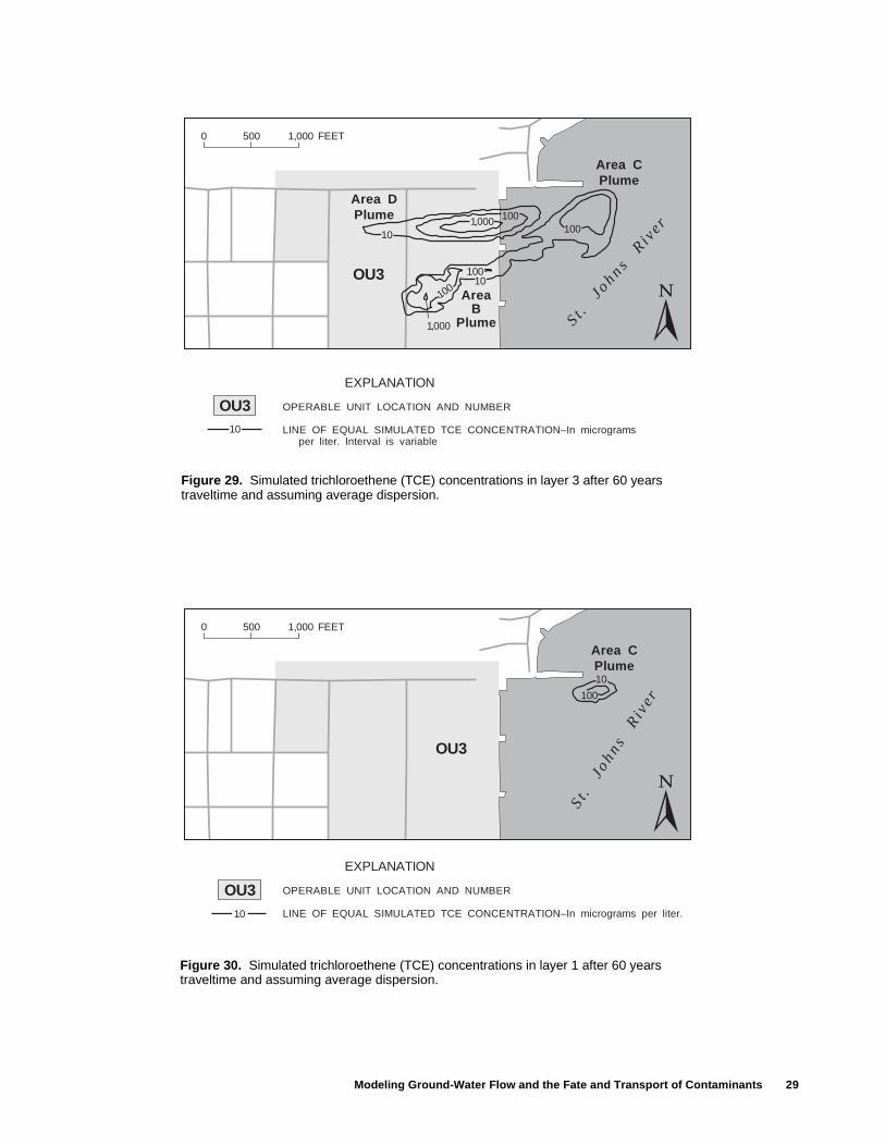
Modeling Ground-Water Flow and the Fate and Transport of Contaminants 29
EXPLANATION
OPERABLE UNIT LOCATION AND NUMBER
LINE OF EQUAL SIMULATED TCE CONCENTRATION–In micrograms per liter.10
St .
Joh
ns
Riv
er
OU3
OU3
0 500 1,000 FEET
100
10
Area CPlume
Figure 30. Simulated trichloroethene (TCE) concentrations in layer 1 after 60 years traveltime and assuming average dispersion.
EXPLANATION
OPERABLE UNIT LOCATION AND NUMBER
LINE OF EQUAL SIMULATED TCE CONCENTRATION–In microgramsper liter. Interval is variable
10
St .
Johns
Riv
er
OU3
OU3
0 500 1,000 FEET
10
100100
100
1,000
1,000
10010
Area DPlume
Area CPlume
AreaB
Plume
Figure 29. Simulated trichloroethene (TCE) concentrations in layer 3 after 60 years traveltime and assuming average dispersion.

30 Fate and Transport Modeling of Selected Chlorinated Organic Compounds at Operable Unit 3, U.S. Naval Air Station, Jacksonville, Florida
EXPLANATION
OPERABLE UNIT LOCATION AND NUMBER
LINE OF EQUAL SIMULATED TCE CONCENTRATION–In micrograms per liter.Interval is variable
10
St .
JohnsR
iver
OU3
OU3
10
10100
100
10
10
1,000
0 500 1,000 FEETArea CPlumeArea D
Plume
Area BPlume
Figure 31. Simulated trichloroethene (TCE) concentrations in layer 3 after 100 years traveltime and assuming average dispersion.
EXPLANATION
OPERABLE UNIT LOCATION AND NUMBER
LINE OF EQUAL SIMULATED TCE CONCENTRATION–In microgramsper liter. Interval is variable
10
St .
JohnsR
iver
OU3
OU3
1,000
100
0 500 1,000 FEET
Area CPlume
Area DPlume
10
Figure 32. Simulated trichloroethene (TCE) concentrations in layer 1 after 100 years traveltime and assuming average dispersion.

Modeling Ground-Water Flow and the Fate and Transport of Contaminants 31
Porosity
Similar to the retardation factor, the effective porosity affects the movement of contaminants in a straightforward manner. If the porosity is doubled, the traveltime of the contaminants is doubled. If the porosity is halved, the traveltime is halved. For example, in figure 23, if the porosity for this simulation had been halved, the contours shown would be for 30 years (the contours would have exactly the same shape and values). Conversely, if the porosity had been doubled, the contours shown would be for 120 years. The porosity used in the simulations was 12.5 percent, and as discussed previously, was determined by matching the location of the Area D plume with its suspected source. This porosity is on the low side when compared to other investigations. Therefore, it is unlikely that the actual aquifer porosity is lower, but it is reasonable that it may be higher. Since a low porosity will give fast traveltimes, the simulations by the model should be conservative (predicting an early arrival at the river), and a most likely upper limit on the traveltime would be double the current simulated values.
Chemical Degradation
Chemical degradation was modeled at Area G because Area G was the only place where the rate of degradation was documented and seemed to be fast enough to substantially reduce contaminant concentra-tion. The estimated half-life for TCE ranged from 3.75 to 13.5 years (U.S. Navy, 1998). Using the slower rate, simulations showed that TCE would degrade before reaching discharge points. Obviously, if the faster rate were used the TCE would decay even quicker. The traveltime to the river for higher concentrations of TCE was about 200 years, assuming no degradation. Thus, even fairly slow rates of degradation would have a long time to act to reduce contaminant levels.
Simulation of Pumping to Remediate Ground-Water Contamination
One of several remedial alternatives that the Navy is considering to prevent the discharge of TCE-contaminated ground water to the St. Johns River is to “pump and treat.” The pumping of ground water from the aquifer was simulated to help assess the effects of such an effort. The pump-and-treat alternative would consist of five wells pumping at 5 gallons per minute (gal/min).
The pump-and-treat simulations assume that all of the contamination is dissolved and that no free prod-uct is present to act as an ongoing source. This was assumed because the concentrations of containments were not high enough to indicate the presence of free product. However, if free product was present then the time necessary to remove the contamination by pump-ing would be increased significantly.
The first step in simulating the effects of pump-ing was to establish reasonable values for the constant head cells at the perimeter of the site-specific model. This was done by rerunning the subregional model with the five wells to determine a new steady-state head distribution. The new heads from the subregional model were then transferred to the site-specific model. The site-specific model was then run with the five pumping wells. The distribution of TCE after 5, 10, and 15 years of pumping are shown in figures 33, 34, and 35, respectively.
The simulated change in concentrations of TCE in ground water pumped from the two wells located at Area C is shown in figure 36. The concentrations trend downward and were below 1 µg/L after about 16 years (fig. 36). Well 3 was turned off after 17 years because a low concentration was attained. Well 4 was allowed to pump longer to capture some TCE that was trapped in a stagnation point that developed between wells 3 and 4.
The simulated change in concentrations of TCE at Area D is shown in figure 37. The concentrations trend downward and were below 1 µg/L after about 18 years (fig. 37). Well 1 was turned off after 11 years because a low concentration was attained. Well 2 initially had an increase in concentration because the well was located slightly downgradient from the high-est concentration in the aquifer. Well 2 had an increase in concentration after well 1 was turned off because a high concentration of TCE was trapped in a stagnation point that occurred between wells 1 and 2. After well 1 was turned off, the TCE moved toward well 2.
Table 6. Range of retardation factors for the upper and intermediate layers of the surficial aquifer
[TCE, trichloroethene; DCE, cis-dichloroethene; VC, vinyl chloride]
Surficial aquifer High Low Average
Upper Layer
TCE 3.3 2.2 2.8
DCE 2.5 1.8 2.2
VC 2.0 1.6 1.8
Intermediate layer
TCE 5.7 1.6 3.8
DCE 4.2 1.4 2.9
VC 3.1 1.3 2.2
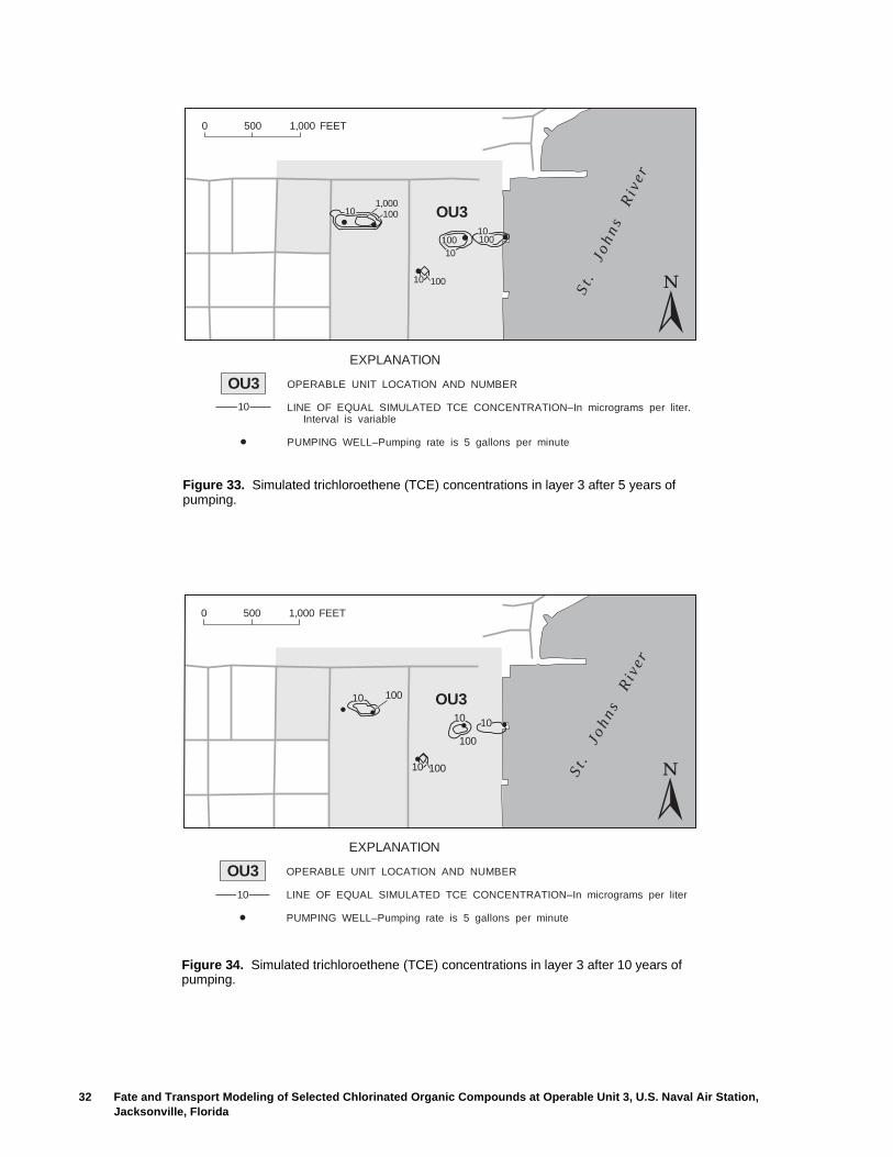
32 Fate and Transport Modeling of Selected Chlorinated Organic Compounds at Operable Unit 3, U.S. Naval Air Station, Jacksonville, Florida
EXPLANATION
OPERABLE UNIT LOCATION AND NUMBER
LINE OF EQUAL SIMULATED TCE CONCENTRATION–In micrograms per liter.Interval is variable
PUMPING WELL–Pumping rate is 5 gallons per minute
10
St .
Jo
hn
sR
ive
r
0 500 1,000 FEET
OU3
OU3
1001,000
10
100
100
10010
10
10
Figure 33. Simulated trichloroethene (TCE) concentrations in layer 3 after 5 years of pumping.
St .
Joh
ns
Riv
er
0 500 1,000 FEET
OU3
OU3
EXPLANATION
OPERABLE UNIT LOCATION AND NUMBER
LINE OF EQUAL SIMULATED TCE CONCENTRATION–In micrograms per liter
PUMPING WELL–Pumping rate is 5 gallons per minute
10
100
100
10
10
10 10
100
Figure 34. Simulated trichloroethene (TCE) concentrations in layer 3 after 10 years of pumping.
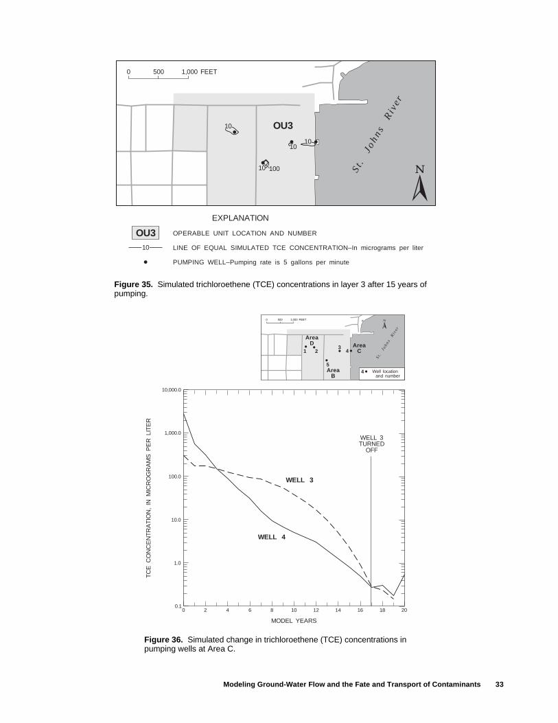
Modeling Ground-Water Flow and the Fate and Transport of Contaminants 33
WELL 3TURNED
OFF
00.1
1.0
10.0
100.0
1,000.0
10,000.0
2 4 6 8 10
MODEL YEARS
12 14 16 18 20
WELL 4
WELL 3
TC
EC
ON
CE
NT
RA
TIO
N,
INM
ICR
OG
RA
MS
PE
RLI
TE
R
21
St .
Joh
ns
Riv
er
0 500 1,000 FEET
321 4
5Well location
and number4
AreaD Area
C
AreaB
Figure 36. Simulated change in trichloroethene (TCE) concentrations in pumping wells at Area C.
St .
Joh
ns
Riv
er
0 500 1,000 FEET
OU3
EXPLANATION
OPERABLE UNIT LOCATION AND NUMBER
LINE OF EQUAL SIMULATED TCE CONCENTRATION–In micrograms per liter
PUMPING WELL–Pumping rate is 5 gallons per minute
10
OU3
10
10
100
10
10
Figure 35. Simulated trichloroethene (TCE) concentrations in layer 3 after 15 years of pumping.

34 Fate and Transport Modeling of Selected Chlorinated Organic Compounds at Operable Unit 3, U.S. Naval Air Station, Jacksonville, Florida
SUMMARY
The U.S. Naval Air Station (referred to as the Station) occupies 3,800 acres adjacent to the St. Johns River in Jacksonville, Florida. The Station was placed on the U.S. Environmental Protection Agency’s National Priorities List in December 1989, and is participating in the U.S. Department of Defense Instal-lation Restoration Program, which serves to identify and remediate environmental contamination in compliance with the Comprehensive Environmental Response, Compensation, and Liability Act and the Superfund Amendments and Reauthorization Act of 1980 and 1985, respectively.
Operable Unit 3 (OU3) occupies 134 acres on the eastern side of the Station. The Naval Aviation Depot, located at OU3, services numerous types of military aircraft. Waste materials spilled or disposed of at OU3 in past years include paint sludges, solvents, battery acids, aviation fuels, petroleum lubricants, and radioactive material. Contamination by the chlorinated
organic compounds trichloroethene (TCE), cis-dichlo-roethene (cis-DCE), and vinyl chloride (VC) have been found in the ground water of the surficial aquifer. The surficial aquifer is exposed at land surface and forms the uppermost permeable unit at the Station. This aquifer is 30- to 100-ft thick and consists of tan to yellow, medium to fine unconsolidated silty sands interbedded with lenses of clay, silty clay, and sandy clay. The surficial aquifer at OU3 is approximately 100-ft thick and consists of two distinct layers. The upper layer is unconfined and extends from land surface to about 10 to15 ft below sea level; the inter-mediate layer is confined and extends from the upper layer downward to the top of the Hawthorn Group. In the northern and central parts of OU3, the upper and intermediate layers are separated by a low-permeability clay layer.
Chlorinated organic compounds were detected at nine “hot spot” areas. Simulating the transport of TCE from four of these Areas (B, C, D, and G) was the emphasis of this investigation. TCE contamination is
WELL 1TURNED
OFF
00.1
1.0
10.0
100.0
1,000.0
10,000.0
2 4 6 8 10
MODEL YEARS
12 14 16 18 20
WELL 1
WELL 2
TC
EC
ON
CE
NT
RA
TIO
N,
INM
ICR
OG
RA
MS
PE
RLI
TE
R
St .
Joh
ns
Riv
er
0 500 1,000 FEET
34
5Well location
and number4
21
AreaD Area
C
AreaB
Figure 37. Simulated change in trichloroethene (TCE) concentrations in pumping wells at Area D.

References 35
located in the intermediate layer of the aquifer at Areas B, C, and D, and in the upper layer at Area G. The rate of degradation of TCE at Areas B, C, and D seems to be slow and the velocity of the ground water is rela-tively fast. As a result, TCE-contaminated ground water may reach the St. Johns River. The rate of degra-dation at Area G seems to be relatively fast, so that TCE-contaminated ground water is unlikely to reach discharge points.
Retardation factors for TCE, cis-DCE, and VC were 2.8, 2.2, and 1.8, respectively, for the upper layer of the surficial aquifer and 3.8, 2.9, and 2.2, respec-tively, for the intermediate layer. These factors were calculated based on average fraction organic carbon contents of 2.185×10⁻³ grams per gram (g/g) for the upper layer and 3.359×10⁻³ g/g for the intermediate layer.
Site-specific ground-water flow modeling was conducted at OU3 using MODFLOW. The site-specific model was of limited aerial extent with a small cell size. A previously developed MODFLOW model was used to establish the boundary conditions for the site-specific model, which contained 98 rows and 108 columns; all model cells were 50 ft on each side. Vertically, the surficial aquifer was divided into four layers.
Solute-transport modeling was conducted using MT3DMS. The solute-transport model used the same grid and layering as the site-specific ground-water flow model. All model simulations were conducted twice, once using low dispersivities and once using average dispersivities. A horizontal dispersivity of 1 ft and transverse and vertical dispersivities of 0.03 ft were used to represent values on the low end of the expected range. A horizontal dispersivity of 7 ft and transverse and vertical dispersivities of 0.18 ft were used to represent average values. An effective porosity of 12.5 percent was used.
Simulations using a low dispersivity, which resulted in the highest TCE concentrations discharging to the St. Johns River, gave the following results. At 60 years traveltime, the highest concentration of TCE associated with the Area C plume had moved under and discharge to the St. Johns River; TCE concentra-tions exceeded 1×10³ µg/L. At 100 years traveltime, the highest concentration of TCE associated with the Area D plume had moved under and discharged to the river; TCE concentrations exceeded 3×10³ µg/L. At 200 years traveltime, the Area B plume had not discharged to the river.
Natural degradation of chlorinated organic compounds has been documented at Area G. Simula-tions using a first-order decay rate half-life of 13.5 years resulted in the TCE plume degrading before the plume reached the St. Johns River. The ratio of the concentrations of TCE to cis-DCE and VC was assumed to remain relatively constant so that break-down products would also fail to reach the river.
Simulations using average dispersivity values gave the following results. At 60 years traveltime, the highest concentration of TCE associated with the Area C plume had discharged to the St. Johns River at a concentration exceeding 4×10² µg/L. At 100 years traveltime, the highest concentration of TCE associ-ated with the Area D plume had discharged to the river at a concentration exceeding 1×10³ µg/L. The Area B plume had not discharged to the river.
“Pump and treat” is under consideration as a remedial alternative to prevent the discharge of TCE-contaminated ground water from reaching the St. Johns River. Five wells pumping 5 gallons per minute were simulated—one well at Area B, and two wells each at Areas C and D. The concentration of TCE at Area B trended rapidly downward; however, one isolated pocket of TCE contamination remained because of low-permeability sediments at this area. The concen-tration of TCE at Area C trended rapidly downward and was below 1 µg/L in about 16 years. The concen-tration of TCE at Area D also trended rapidly down-ward and was below 1 µg/L in about 18 years.
REFERENCES
Brooks, H.K., 1981, Physiographic divisions, State of Flor-ida: University of Florida, Center for Environmental and Natural Resources Programs, 1 sheet.
Davis, J. H., Planert, M., and Andrews, W.J., 1996, Simula-tion of ground-water flow at the U.S. Naval Air Station, Jacksonville, Florida, with an evaluation of changes to ground-water flow caused by proposed remedial designs at Operable Unit 1: U.S. Geological Survey Open-File Report 96-597, 47 p.
Davis, J.H., 1998, Ground-water hydrology and simulation of ground-water flow at Operable Unit 3 and surround-ing region,U.S. Naval Air Station, Jacksonville, Florida: U.S. Geological Survey Open-File Report 98-68, 36 p.
Fairchild, R.W., 1972, The shallow-aquifer system in Duval County, Florida: Tallahassee, Florida Bureau of Geol-ogy Report of Investigations no. 59, 50 p.

36 Fate and Transport Modeling of Selected Chlorinated Organic Compounds at Operable Unit 3, U.S. Naval Air Station, Jacksonville, Florida
Gelhar, L.W., Welty, C., and Rehfeldt, K.R., 1992, A critical review of data on field-scale dispersion in aquifers: Water Resources Research, v. 28, no 7, 19 p.
Hillel, D., 1980, Fundamentals of soil physics, Academic Press, Inc., 413 p.
Hseih, P. A., and Freckleton, J. R., 1993, Documentation of a computer program to simulate horizontal-flow barri-ers using the U.S. Geological Survey’s modular three-dimensional finite-difference ground-water flow model: U.S. Geological Survey Open-File Report 92-477, 32 p.
McDonald, M.G., and Harbaugh, A.W., 1988, A modular three-dimensional finite-difference ground-water flow model: U.S. Geological Survey Techniques of Water-Resources Investigations, book 6, chap. A1, variously paged.
Mercer, J.W., Skipp, D.C., and Griffin, D., 1990, Basic pump-and-treat ground-water remediation technology: U.S. Environmental Protection Agency, EPA/600/8-90/003.
Miller, J.A., 1986, Hydrogeologic framework of the Flori-dan aquifer system in Florida, and in parts of Georgia, Alabama, and South Carolina: U.S. Geological Survey Professional Paper 1403-B, 91 p.
Scott, T.M., 1988, The lithostratigraphy of the Hawthorn Group (Miocene) of Florida: Tallahassee, Florida Geological Survey Bulletin no. 59, 148 p.
U.S. Navy Department, Southern Division, Naval Facilities Engineering Command, 1994a, Remedial investigation and feasibility study, Operable Unit 3, Naval Air Sta-tion, Jacksonville: South Division Contract N62467-89-D-0317, 142 p.
----- 1994b, Engineering evaluation and cost analysis build-ings 106 and 780 at Operable Unit 3, Naval Air Station, Jacksonville: South Division Contract N62467-89-D-0317/076, 48 p.
----- 1998, Engineering evaluation of areas with elevated groundwater contamination, Operable Unit 3, Naval Air Station, Jacksonville: South Division Contract N62467-89-D-0317/076, 107 p.
Zheng, C, and Bennett, G. D., 1995, Applied contaminant transport modeling, theory and practice: New York, Van Nostrand Reinhold, 440 p.
Zheng, C, and Wang, Patrick, 1998, MT3DMS Documenta-tion and user’s guide: Tuscaloosa, Ala., Departments of Geology and Mathematics, University of Alabama, 185 p.