Fatality Reduction by Safety Belts

U.S. Departmentof Transportation http://www.nhtsa.dot.gov

National HighwayTraffic Safety Administration

DOT HS 809 199 December 2000 NHTSA Technical Report

Fatality Reduction by Safety Beltsfor Front-Seat Occupantsof Cars and Light Trucks

Updated and Expanded EstimatesBased on 1986-99 FARS Data

This document is available to the public from the National Technical Information Service, Springfield, Virginia 22161.

The United States Government does not endorse products ormanufacturers. Trade or manufacturers’ names appear onlybecause they are considered essential to the object of this report.

Technical Report Documentation Page1. Report No.

DOT HS 809 199

2. Government Accession No. 3. Recipient’s Catalog No.

4. Title and Subtitle

FATALITY REDUCTION BY SAFETY BELTS FORFRONT-SEAT OCCUPANTS OF CARS AND LIGHT TRUCKSUpdated and Expanded Estimates Based on 1986-99 FARS Data

5. Report Date

December 20006. Performing Organization Code

7. Author(s)

Charles J. Kahane, Ph.D.

8. Performing Organization Report No.

9. Performing Organization Name and Address

Evaluation Division, Plans and PolicyNational Highway Traffic Safety AdministrationWashington, DC 20590

10. Work Unit No. (TRAIS)

11. Contract or Grant No.

12. Sponsoring Agency Name and Address

Department of TransportationNational Highway Traffic Safety AdministrationWashington, DC 20590

13. Type of Report and Period Covered

NHTSA Technical Report14. Sponsoring Agency Code

15. Supplementary Notes

16. Abstract

The National Highway Traffic Safety Administration estimated in 1984 that manual 3-point safety beltsreduce the fatality risk of front-seat occupants of passenger cars by 45 percent relative to the unrestrainedoccupant. The agency still relies on that estimate. Shortly after 1985, the prime analysis technique forFatality Analysis Reporting System (FARS) data, double-pair comparison, began producing inflated,unreliable results. This report develops an empirical tool to adjust double-pair comparison analyses of1986-99 FARS data. It validates the adjustments by comparing the belt use of fatally injured people incertain types of crashes to belt use observed on the road in State and national surveys. These methodsreconfirm the agency’s earlier estimates of fatality reduction by manual 3-point belts: 45 percent inpassenger cars and 60 percent in light trucks. Furthermore, they open the abundant 1986-99 FARS data toadditional analyses, permitting point-estimation of belt effectiveness by crash type, occupant age andgender, belt type, vehicle type, etc.

17. Key Words

safety belt; occupant protection; fatal crash;crashworthiness; FARS; fatality reduction;statistical analysis; evaluation; frontal impact; sideimpact; rollover; ejection; belt use; automatic belt

18. Distribution Statement

Document is available to the public through theNational Technical Information Service, Springfield,Virginia 22161

19. Security Classif. (Of this report)

Unclassified

20. Security Classif. (Of this page)

Unclassified

21. No. of Pages

77

22. Price

Form DOT F 1700.7 (8-72) Reproduction of completed page authorized

TABLE OF CONTENTS

1. History of the effectiveness estimates . . . . . . . . . . . . . . . . . . . . . . . . . . . . . . . . . . . . . . . . . . . 1

2. Goals of this report . . . . . . . . . . . . . . . . . . . . . . . . . . . . . . . . . . . . . . . . . . . . . . . . . . . . . . . . 4

3. “Classic” double-pair comparison: passenger cars in CY 1977-85 . . . . . . . . . . . . . . . . . . . . . 6

4. Inflated results for passenger cars in CY 1986-99 . . . . . . . . . . . . . . . . . . . . . . . . . . . . . . . . 10

5. The “universal exaggeration factor” (UEF) and its robustness . . . . . . . . . . . . . . . . . . . . . . . 13

6. A refined effectiveness estimate - controlling for crash mode . . . . . . . . . . . . . . . . . . . . . . . . 20

7. Sampling error considerations . . . . . . . . . . . . . . . . . . . . . . . . . . . . . . . . . . . . . . . . . . . . . . . 22

8. RESULTS: BELT EFFECTIVENESS ESTIMATES . . . . . . . . . . . . . . . . . . . . . . . . . . . . . 26

9. Validation: belt use of fatalities vs. observed on the road . . . . . . . . . . . . . . . . . . . . . . . . . . . 43

References . . . . . . . . . . . . . . . . . . . . . . . . . . . . . . . . . . . . . . . . . . . . . . . . . . . . . . . . . . . . . . . . 71

Appendix: State belt use surveys and laws, 1991-99 . . . . . . . . . . . . . . . . . . . . . . . . . . . . . . . . . 75

iii

1Final Regulatory Impact Analysis, Amendment to Federal Motor Vehicle SafetyStandard 208, Passenger Car Front Seat Occupant Protection, NHTSA Publication No. DOTHS 806 572, Washington, 1984, pp. IV-1 - IV-16.

2Fourth Report to Congress, Effectiveness of Occupant Protection Systems and their Use,NHTSA Publication No. DOT HS 808 919, Washington, 1999, pp. 11-12.

3Safety Belt Usage, A Review of Effectiveness Studies, Suggestions for State Programs,NHTSA Publication No. DOT HS 801 988, Washington, 1976, p. 1.

4Partyka, Susan C., “Seat Belt Effectiveness Estimates Using Data Adjusted for DamageType (January 1984),” Papers on Adult Seat Belts - Effectiveness and Use, NHTSA PublicationNo. DOT HS 807 285, Washington, 1988, pp. 1-12. Kahane, Charles J., Addendum to "Seat BeltEffectiveness Estimates Using Data Adjusted for Damage Type”, NHTSA Docket No. 74-14-N35-229-05, 1984.

5Final Regulatory Impact Analysis (1984), pp. IV-14 - IV-15.

1

1. HISTORY OF THE EFFECTIVENESS ESTIMATES

In 1984, the National Highway Traffic Safety Administration (NHTSA) issued its automaticprotection requirement for passenger cars. The agency’s regulatory impact analysis estimated thatmanual 3-point safety belts, when used by drivers or right-front passengers of cars, reduce fatalityrisk by approximately 45 percent relative to the unrestrained occupant1. The effectiveness wasalso stated as an interval estimate: 40 to 50 percent. These numbers became, and still remain2 theagency’s “official” estimates of belt effectiveness in cars. They were a retrenchment from theagency’s 1976 estimate of 60 percent3 and even higher numbers elsewhere in the literature thathad been based on relatively simple comparisons of fatality rates per 100 belted and unrestrainedoccupants.

The 45 percent estimate (or 40-50 percent range) was the agency’s consensus and best judgementbased on two types of analyses:

C Recognition that people who buckled up were involved in less severe crashes than peoplewho did not use belts (at least in those days). Conscientious efforts to “adjust” or“control” fatality rates per 100 occupants for differences in crash severity produced pointestimates of overall effectiveness in the 39-49 percent range4 (with a substantially widerrange if sampling error is included). In other words, a belted occupant was 39-49 percentless likely to die than an unrestrained person in a crash of the same severity.

C A reality check based on 11 countries and Canadian provinces that had enacted belt uselaws. In each case, the observed increase in belt use and the actual reduction in occupantfatalities after the law were employed to estimate the implicit belt effectiveness. Theseestimates varied considerably (because belt laws often coincided with economic up- ordown-swings in those volatile times) but averaged to 47 percent5.

6Evans, Leonard, “Double Pair Comparison - A New Method to Determine HowOccupant Characteristics Affect Fatality Risk in Traffic Crashes,” Accident Analysis andPrevention, Vol. 18, June 1986, pp. 217-227. Evans, Leonard, “The Effectiveness of Safety Beltsin Preventing Fatalities,” Accident Analysis and Prevention, Vol. 18, June 1986, pp. 229-241.

7Partyka, Susan C., “Belt Effectiveness in Pickup Trucks and Passenger Cars by CrashDirection and Accident Year (May 1988),” Papers on Adult Seat Belts - Effectiveness and Use,NHTSA Publication No. DOT HS 807 285, Washington, 1988, pp. 99-102.

8Ibid., p. 99 and p. 102.

9Traffic Safety Facts 1998, NHTSA Publication No. DOT HS 808 983, Washington,1999, p. 186.

2

These analyses made the previous 60+ percent estimates unrealistic and supported the 40-50percent range.

Within two years, Leonard Evans published his influential double-pair comparison analyses of1975-83 FARS data, showing a 41 percent fatality reduction by 3-point belts in passenger cars,with 2-sigma confidence bounds ± 8 percent6. Double-pair comparison (which will be definedwith examples in Section 3) is valuable because it allows the direct use of FARS data that have amuch higher N of fatalities than NASS or state files. A second major advantage is that double-pair comparison implicitly “adjusts” or “controls” for the differences in the severity of crashesinvolving belted and unrestrained occupants. The 41 percent effectiveness estimate was withinthe agency’s 40-50 percent range and, together with the two preceding analyses provided a strongfoundation for the agency’s position.

Analysts at NHTSA and elsewhere quickly adopted double-pair comparison for analyzing beltsand other safety devices. However, Susan Partyka and others soon noted that belt effectivenessestimates rose substantially as more recent FARS data were fed into the analyses. For example,analyses of 1982-87 FARS data produced a belt effectiveness estimate of 55 percent for passengercars7. After perhaps a little wishful thinking that earlier estimates might have been low by chancealone, or even that belts might have become more effective, NHTSA staff soon concluded thatsomething had gone wrong with belt use reporting on FARS (and other files) and had biasedeffectiveness estimates upwards8.

Specifically, New York was the first state to enact a belt use law, effective December 1, 1984. After a brief “wait and see,” 21 states, including 9 of the 10 most populous states had belt lawseffective by August 1986 for front-seat occupants of passenger cars9. For the first time, unbeltedpeople had a tangible incentive - avoidance of a fine - to report that they were belted. NHTSAhypothesized that:

C Uninjured or slightly injured occupants are often up and about before police arrive at thecrash scene. Since the investigating officer is not an eye-witness to their belt use, theyhave an opportunity, and now also a motive, to say they wore belts, even if they hadn’t.

10Partyka, Susan C., Lives Saved by Seat Belts from 1983 through 1987, NHTSAPublication No. DOT HS 807 324, Washington, 1988.

3

C Mortally injured occupants may be in their original post-crash location when police arrive,often allowing direct observation of belt use.

Thus, NHTSA believes belt use of fatalities is reported without net biases on FARS before andafter belt laws10. However, after the laws, belt use of survivors is overreported. A bias hasapparently been introduced in the reporting of this one data element, for survivors, as aconsequence of belt use laws. It has occurred despite the long-term, ongoing efforts by NHTSAand the states in data quality control and analyst training, which have resulted in more accurate,complete and consistent information on most FARS data elements.

When survivors who were actually unrestrained are reported as belted, it lowers the fatality oddsin the “belted” population, raises the odds in the “unrestrained” population, and bloats theeffectiveness estimate. The following hypothetical example shows how. For simplicity, it is basedon fatality rates per 100 crash-involved occupants, as might be derived from state crash files. However, the same type of bias would occur in a double-pair comparison analysis.

First, if belt use had been accurately reported by everyone, there would have been a population of100 unrestrained and 100 belted occupants, with a fatality rate 45 percent lower for the beltedoccupants than for the unrestrained:

Based on Actual Belt Use

Not FatalityBelted Belted Reduction

Fatalities 20 11Survivors 80 89Total 100 100Fatality rate .20 .11 45%

The “fatality reduction,” 45 percent = 1 - (.11/.20) = 1 - (belted fatality rate/unbelted fatality rate). If 15 of the unrestrained survivors misreported themselves as “belted” (while all the fatalitiescontinue to be correctly reported), the fatality rate for reportedly “unrestrained” people increasesand the “belted” fatality rate decreases:

11Partyka, “Belt Effectiveness in Pickup Trucks and Passenger Cars by Crash Directionand Accident Year,” op. cit.

12Preliminary Regulatory Impact Analysis, Proposed Extension of the AutomaticRestraint Requirements of FMVSS 208 to Trucks, Buses and Multi-Purpose Passenger Vehicleswith a Gross Vehicle Weight Rating of 8,500 Pounds or Less and an Unloaded Vehicle Weight of5,000 Pounds or Less, NHTSA Docket No. 74-14-N62-001, 1989, p. 15.

4

Based on Reported “Belt Use”

“Not FatalityBelted” “Belted” Reduction

Fatalities 20 11Survivors 80 - 15 = 65 89 + 15 = 104Total 100 - 15 = 85 100 + 15 = 115Fatality rate .24 .10 59%

The fatality reduction is inflated from a true 45 percent to an observed 59 percent.

The agency reached a decision point in 1989 when it extended automatic protection to lighttrucks. For the regulatory impact analysis, the agency needed to estimate the effectiveness ofmanual belts. Partyka’s double-pair comparison (based on FARS data through 1987) showed a69 percent fatality reduction for belts in pickup trucks11. The regulatory impact analysis assertedthat this result was inflated. Since Partyka’s data showed a 55 percent reduction in passengercars, whereas the agency believed 45 percent was the true reduction, the light truck estimateought to be scaled back by a similar amount: from 69 to 60 percent12. In the process, the agency:

C Reconfirmed the 45 percent estimate for cars and established a 60 percent estimate forlight trucks.

C Asserted that FARS analyses producing estimates higher than those were biased and oughtnot be accepted at face value.

2. GOALS OF THIS REPORT

Eleven years later, as of December 2000, the agency continues to rely on 45 and 60 percentestimates that are essentially based on 1975-85 data and 1975-85 vehicles. Abundant later FARSdata, with much higher N’s of belted fatality cases, remain untapped. The numbers could havebecome outdated as belt systems, vehicles and the crash environment changed. The old data donot allow estimates of post-1985 belt configurations, such as automatic belts or belts in vehicleswith air bags. The old data are too small a sample for accurate estimation of belt effectiveness in

13Kahane, Charles J., Evaluation of FMVSS 214 - Side Impact Protection: DynamicPerformance, NHTSA Publication No. DOT HS 809 004, Washington, 1999, pp. 15-16.

5

important subgroups of crashes, such as specific crash types, occupant age groups, vehicle types,etc.

The objectives of this paper are:

C To develop an empirical tool to adjust for the biases in double-pair comparison analyses oflater FARS data, and open up those FARS files for point estimates of fatality reductionconsistent with pre-1986 results.

C To obtain detailed point estimates of belt effectiveness by crash mode, occupant agegroup, etc., needed for NHTSA regulatory analyses and evaluations, and not reallyavailable from the limited pre-1986 data.

C To obtain point estimates of belt effectiveness for configurations that did not exist before1986, such as automatic belts, or manual belts in vehicles with dual air bags. Theseestimates, too, are needed for regulatory analyses and evaluations.

C To see if belt effectiveness has changed in the newer vehicles, or has changed over time inresponse to an evolving crash environment.

C To see if NHTSA’s long-standing estimates of 45 percent fatality reduction in cars and 60percent in light trucks are still appropriate.

However, the point estimates of this report, relying on several critical assumptions, are not likecustomary statistical estimates derived directly from the data. The uncertainty in our estimates,although it can be discussed to some extent, cannot be fully quantified, based on statistical theory,as “confidence bounds.”

3. “CLASSIC” DOUBLE-PAIR COMPARISON: PASSENGER CARS IN CY 1977-85

Evans, Partyka and others have provided detailed examples of double-pair comparison analyses inthe literature, but let us run through one case here from start to finish, both as a review and todemonstrate the specific estimation procedure used in this report.

The starting point for this analysis is FARS data for CY 1977-85. Records of passenger cars ofmodel years 1975-86 are extracted (1975 is the first model year with “Type 2" 3-point beltsystems, not counting 1974 where cars were also equipped with the ignition interlock). “Passenger cars” in MY 1975-80 are all FARS vehicle records with the variable BODY_TYP= 1-9, and in MY 1981-86 are the cases with decodable VINs that are passenger cars accordingto the VIN decode program developed for NHTSA evaluations13. The analysis is limited to:

6

C Cars with a driver and a right front (RF) passenger (and perhaps other passengers). Whentwo or more people occupy the same seat, according to FARS, only the occupant with thelowest PER_NO (person number) is included.

C The driver, or the RF passenger, or both were fatally injured.

C The driver and the RF passenger both have known reported belt use: MAN_REST has tobe 0 (unrestrained) or 1, 2, 3, 8 or 13 (belted, perhaps incorrectly).

C The driver and the RF passenger are both 14 to 97 years old.

There are 30,665 cars in CY 1977-85 with a driver and a RF passenger, at least one fatal, bothwith known belt use and 14-97 years old. The vehicle cases tabulate as follows, based on eachoccupant’s belt use and survival:

Vehicles Driver Died Driver Survived BothRF Survived RF Died Died

Both unrestrained 11,186 11,469 5,317Driver unrestrained, RF belted 300 152 74Driver belted, RF unrestrained 186 487 102Both belted 497 653 242

This can be tabulated as fatality rather than vehicle cases, by adding the “both died” column toeach of the preceding columns:

Fatalities Driver RF Driver/RFFatalities Fatalities Risk Ratio

Both unrestrained 16,503 16,786 0.983Driver unrestrained, RF belted 374 226 1.655Driver belted, RF unrestrained 288 589 0.489Both belted 739 895 0.826

In CY 1977-85, it is clear that (1) the overwhelming majority of people killed in crashes wereunrestrained; (2) unrestrained drivers and RF passengers are at nearly equal risk in the same crash;and (3) whoever buckled up substantially reduced their risk.

The four rows of data allow a total of four double-pair comparisons, two for computing theeffectiveness of belts for drivers, and two for RF passengers. The first comparison for the driveris based on the first and third rows of data:

7

Driver RF Driver/RFFatalities Fatalities Risk Ratio

Driver unrestrained RF unrestrained 16,503 16,786 0.983Driver belted RF unrestrained 288 589 0.489

In both pairs, the driver’s fatality risk is compared to the same control group: the unrestrained RFpassenger. The unrestrained driver has essentially the same fatality risk as the unrestrained RF inthe same crash, the belted driver about half. The fatality reduction for belts is

1 - (0.489/0.983) = 50.3 percent.

The other comparison for the driver is based on the second and fourth rows of data:

Driver RF Driver/RFFatalities Fatalities Risk Ratio

Driver unrestrained RF belted 374 226 1.655Driver belted RF belted 739 895 0.826

Here, the control group is the belted RF passenger. The unrestrained driver has higher fatalityrisk than the belted RF in the same crash, the belted driver, lower. The fatality reduction is:

1 - (0.826/1.655) = 50.1 percent.

It is important that the effectiveness estimates are nearly identical with the two control groups: itsuggests the estimates are robust and not affected by the choice of control group.

The first double-pair comparison for estimating belt effectiveness for the RF passenger is obtainedby using the first two rows of data, reversing the order of the columns and computing theRF/Driver rather than the Driver/RF risk ratio:

RF Driver RF/DriverFatalities Fatalities Risk Ratio

RF unrestrained Driver unrestrained 16,786 16,503 1.017RF belted Driver unrestrained 226 374 0.604

The control group is the unrestrained driver. The fatality reduction for the belted RF passengeris:

8

1 - (0.604/1.017) = 40.6 percent.

The second estimate uses the last two rows of data:

RF Driver RF/DriverFatalities Fatalities Risk Ratio

RF unrestrained Driver belted 589 288 2.045RF belted Driver belted 895 739 1.211

The control group is the belted driver. The fatality reduction for the belted RF passenger is:

1 - (1.211/2.045) = 40.8 percent.

Again, the two control groups produce nearly identical estimates. Also, as in earlier studies, belteffectiveness is lower for the RF passenger than for the driver.

The next task is to develop a weighting procedure that combines the two driver estimates into asingle number, and likewise for the two RF estimates.

In the 1977-85 FARS data, the actual number of driver fatalities is

Actual driver fatalities = 16,503 + 374 + 288 + 739 = 17,904

The first two numbers in that sum are unrestrained drivers, the last two, belted. However, ifevery driver had been unrestrained, that sum would have increased to

All-unrestrained driver fatalities = 16,503 + 374 + (0.983 x 589) + (1.655 x 895) = 18,937

(Here, 589 was the number of unrestrained RF fatalities that accompanied the 288 belted driversand 0.983 is the risk ratio of unrestrained driver to unrestrained RF fatalities; 895 is the number ofbelted RF fatalities that accompanied the 739 belted drivers and 1.655 is the risk ratio ofunrestrained drivers to belted RF fatalities.)

On the other hand, if every driver had buckled up, the sum would have dropped to

All-belted driver fatalities = (0.489 x 16,786) + (0.826 x 226) + 288 + 739 = 9,421

The overall effectiveness of belts for drivers is

(18,937 - 9,421) / 18,937 = 50.25 percent,

9

which is between the results of the two separate double-pair comparisons for drivers (50.1 and50.3 percent).

Similarly, the actual number of RF passenger fatalities is

Actual RF fatalities = 16,786 + 226 + 589 + 895 = 18,496

If every RF passenger had been unrestrained, that sum would have increased to

All-unrestrained RF fatalities = 16,786 + (1.017 x 374) + 589 + (2.045 x 739) = 19,267

(Here, 374 was the number of unrestrained driver fatalities that accompanied the 226 belted RFpassengers and 1.017 is the risk ratio of unrestrained RF to unrestrained driver fatalities; 739 isthe number of belted driver fatalities that accompanied the 895 belted RF and 2.045 is the riskratio of unrestrained RF to belted driver fatalities.)

But if every RF passenger had buckled up, the sum would have dropped to

All-belted RF fatalities = (0.604 x 16,503) + 226 + (1.211 x 288) + 895 = 11,442

The overall effectiveness of belts for RF passengers is

(19,267 - 11,442) / 19,267 = 40.61 percent,

which is between the results of the two separate double-pair comparisons for RF passengers (40.6and 40.8 percent).

Finally, for an estimate of the overall effectiveness of 3-point belts for front-outboard occupantsof passenger cars, we must note that drivers have over the years typically outnumbered RFpassengers by very close to 3 to 1 in the general crash-involved population (as opposed to thesespecial cases that were limited to cars with the RF seat occupied). The preceding statistics fordrivers need to be weighted by 3 and the statistics for RF passengers by 1. If all drivers and RFpassengers were unrestrained, that sum would have increased to

All-unrestrained front-outboard fatalities = (3 x 18,937) + 19,267 = 76,078

If they had all buckled up, the sum would have dropped to

All-belted front-outboard fatalities = (3 x 9,421) + 11,442 = 39,706

The overall effectiveness of 3-point belts for front-outboard occupants is

(76,078 - 39,706) / 76,078 = 47.81 percent,

10

which is between the estimates for drivers and RF passengers, but closer to the driver estimate, asit should be, given the higher weight factor for drivers.

4. INFLATED RESULTS FOR PASSENGER CARS IN CY 1986-99

Let us repeat the double-pair comparison analysis for passenger cars equipped with 3-point belts,but using more recent FARS data, specifically 1986-99.

Records of passenger cars of model years 1975-99 equipped with 3-point belts are extracted from1986-99 FARS files. “Passenger cars” in MY 1975-80 and 1999 are all FARS vehicle recordswith BODY_TYP 1-9, and in MY 1981-98 are the cases with VINs that decode as passengercars. “Three-point belts” include manual or automatic (door-mounted) 3-point belts, in cars withno air bags or dual air bags. Cars with only a driver air bag are excluded to preserve thesymmetry (nearly equal fatality risk) of the driver and the RF positions in the analysis. As inSection 3, the analysis is limited to cars with a driver and a right front (RF) passenger, both withknown reported belt use, both age 14-97, at least one and perhaps both fatally injured. There are70,668 cars in the 1986-99 files meeting those criteria. The basic tabulation of fatalities is:

Fatalities Driver RF Driver/RFFatalities Fatalities Risk Ratio

Both unrestrained 23,476 23,579 0.996Driver unrestrained, RF belted 3,934 1,622 2.425Driver belted, RF unrestrained 1,815 4,820 0.377Both belted 11,225 12,901 0.870

Relative to the CY 1977-85 data in Section 3, (1) the number of cases in the cells with belteddrivers and/or passengers is an order of magnitude larger - there are a lot more data to work withhere; (2) the effect of belts appears far more dramatic at first glance - the ratio of unrestraineddriver to belted RF fatalities increased from 1.655 to 2.425 while the ratio of belted driver tounrestrained RF decreased from 0.489 to 0.377. Working through the double-pair comparisonsand weighted averages as in Section 3 produces fatality reduction estimates of

63.26 percent for drivers57.71 percent for RF passengers61.89 percent for all front-outboard occupants

These are substantially higher than the corresponding reductions in 1977-85: 50 percent fordrivers, 41 percent for RF passengers and 48 percent combined. They raise three questions:

C When, and how quickly did the observed effectiveness escalate?

14Traffic Safety Facts 1998, op. cit., p. 186.

15A possible alternative approach would be to limit the “pre-law” period to 1977-84, retainthe “post-law” period as 1986-99, and to exclude the 1985 data from the analysis. The observedfatality reduction for 3-point belts in passenger cars is 44.69 percent in 1977-84, as compared to47.81 percent in 1977-85. This would have raised the UEF, as defined in Section 5, from 1.369to 1.452.

11

C Could a substantial part of the increase be due to real improvements in the life-savingeffectiveness of belts in later-model cars?

C Could a substantial part of the increase be due to changes in the crash environment that haveincreased the types of crashes where belts are most effective?

When a separate double-pair comparison analysis is run on each individual calendar year of FARSdata, the observed overall fatality reductions for belts are the following:

1977 49 percent1978 281979 441980 381981 521982 531983 381984 46

1985 55

1986 611987 581988 611989 631990 691991 621992 60

1993 601994 641995 631996 651997 581998 621999 59

The effectiveness results are also graphed in Figure 1.

During 1977-84, observed belt effectiveness varies a fair amount from year to year, due to the smallN’s of belted cases on FARS, but arguably centers on about 45 percent with little or no time trend. In 1986, the first year with belt use laws covering a large proportion of occupants (including 9 of the10 most populous states) the fatality reduction has already reached 61 percent, essentially the 1986-99 average, and it stayed close to that year after year, with no evidence of any time trend within1986-99. The year 1985 is hard to place: the 55 percent is higher than any preceding year, but justbarely higher, for example, than the 53 percent in 1982. It is lower than any subsequent year,although not much lower than the 58 percent in 1987 and 1997. Since belt use laws were justgetting started in a few states in 1985, but were well established in 198614, it seems most appropriateto include the 1985 data with the “pre-law” period15.

In any case, the escalation in the belt effectiveness estimate obviously coincided with the inception ofbelt use laws. The escalation came all at once, with little subsequent change. That not only answersthe first question (when and how quickly) but essentially the other two. If any substantial

12

FIGURE 1

OBSERVED EFFECTIVENESS OF 3-POINT BELTS IN CARS BY CALENDAR YEAR

OBSERVED FATALITYREDUCTION (%) 70 + | ! | | | 65 + ! | ! | ! ! | ! ! | ! ! 60 + ! ! | ! | ! ! | | 55 + ! | | ! | ! | 50 + |! | | | ! 45 + | ! | | | 40 + | | ! ! | | 35 + \ 28 + ! -+--+--+--+--+--+--+--+--+--+--+--+--+--+--+--+--+--+--+--+--+--+--+ 7 7 7 8 8 8 8 8 8 8 8 8 8 9 9 9 9 9 9 9 9 9 9 7 8 9 0 1 2 3 4 5 6 7 8 9 0 1 2 3 4 5 6 7 8 9

CALENDAR YEAR

13

part of the escalation had been due to genuine improvements in belts, that part would have beengradual, since late-model cars with the improved belts only gradually replace the older cars in theoverall vehicle population. The impact of changes in the crash environment would also have beengradual, not abrupt. It is most plausible to conclude that the escalation beginning in 1986 is in factdue to belt use laws resulting in overreporting of belt use by crash survivors, and that ordinarydouble-pair comparison analysis stopped producing accurate estimates of belt effectiveness in 1986.

A comparison of observed effectiveness by calendar year and model year provides additionalevidence that the escalation is due to changes in the data rather than changes in the vehicles:

Observed Fatality Reductions for 3-point Belts in Passenger Cars

Effect in Effect in1977-85 FARS 1986-99 FARS

Manual belts in MY 1975-79 cars 48 63Manual belts in MY 1980-85 cars 47 63Manual belts in MY 1986-90 cars 60Automatic 3-point belts (MY 1987-95) 64Manual belts in cars with dual air bags (MY 1987-99) 63

In the 1977-85 FARS data, belt effectiveness is nearly the same for MY 1975-79 and MY 1980-85cars. In the 1986-99 FARS data, belt effectiveness is essentially the same in all cohorts of vehiclemodel years (and higher than the corresponding numbers for 1977-85 FARS).

5. THE “UNIVERSAL EXAGGERATION FACTOR” (UEF) AND ITS ROBUSTNESS

The two basic results so far are that 3-point belts reduced fatality risk in passenger cars by 47.81percent in 1977-85 FARS data and were observed to “reduce” fatality risk by 61.89 percent in 1986-99 FARS data. The hypothesis is that the first estimate (give or take some “fine tuning” described inSection 6, and sampling error) is an unbiased estimate of the genuine fatality reduction for belts,whereas the second is biased upwards by inaccurate belt use reporting of survivors in FARS inresponse to belt use laws.

Let us define the “Universal Exaggeration Factor” (UEF) to be the relative difference of the twoestimates:

UEF = (100 - 47.81) / (100 - 61.89) = 1.369

16A possible alternative approach, since the CY 1977-85 data contain almost exclusivelyMY 1975-85 cars [with just a few early MY 1986 cars] would be to limit the analysis of 1986-99to MY 1975-85 cars, too. The observed fatality reduction for 3-point belts in MY 1975-85passenger cars is 62.90 percent in CY 1986-99, as compared to 61.89 percent for all MY 1975-2000 cars with 3-point belts in CY 1986-99. This would have raised the UEF from 1.369 to1.407.

14

It is the adjustment factor that has to be applied to the inappropriately low 1986-99 ratio of“belted” to “unbelted” fatality risk to obtain the accurate 1975-85 ratio of actual belted to unbeltedfatality risk:

1.369 x (100 - 61.89) = 100 - 47.81

47.81 = 100 - [1.369 x (100 - 61.89)]

This UEF derives from the effectiveness estimates for 3-point belts in passenger cars, in all types ofcrashes, based on direct double-pair comparison analyses16. Our hypothesis is that this same UEF= 1.369 is also empirically valid for other double-pair comparison analyses based on 1986-99FARS data, including other types of vehicles or belts, subgroups of crashes or occupants, andmore complex weighted averages of double-pair comparisons. In other words, if the analysis of1986-99 data yields an effectiveness estimate E*, the true effectiveness E is close to

E = 100 - [1.369 x (100 - E*)]

If this working hypothesis is acceptable, it would greatly increase the utility of double-paircomparison analysis. Since the 1986-99 FARS data contain an order of magnitude more beltedcases than the 1977-85 data, we will have enough data to obtain effectiveness estimates for specificsubgroups of interest (crash modes, occupant age groups, etc.). We will also be able to obtaineffectiveness estimates for current vehicle types that did not exist in 1977-85 (e.g., belteffectiveness in vehicles with dual air bags). The UEF should be viewed as an empirical tool forgenerating needed point estimates and not as a statistical method that will produce confidencebounds for those estimates.

The hypothesis can be tested (not in a formal, statistical sense) by performing double-paircomparison analyses for selected subsets of the 1977-85 data and the corresponding subsets of the1986-99 data. For each of the subsets, we will compute the exaggeration factor EF of the 1986 -99 effectiveness over the 1977-85 estimate, and compare it to the UEF = 1.369. We can acceptthe hypothesis that 1.369 is a “universal” exaggeration factor if the EF’s for the various subsets areall “relatively” close to 1.369, but not if they differ “a lot” from subset to subset. One factor thatcomplicates the testing is that the EF’s themselves, including the UEF, are statistics and subject tosampling error. Specifically, the 1977-85 FARS data contain relatively few belted cases. Whenthe data are subdivided the 1977-85 effectiveness estimates become quite imprecise, and so will theEF’s. After all, if the 1977-85 data were adequate for precise estimation of belt effectiveness insmall subsets, it would take away a prime motivation for analyzing the 1986-99 data.

15

The first step in testing the UEF is to measure its variation in randomly selected subsets of thedata. For example, FARS data can be split into 10 systematic random subsamples of equal sizebased on the last digit of the case identification number ST_CASE. If separate double-paircomparison analyses are performed on the 10 subsamples of 1977-85 and 1986-99 data, theeffectiveness estimates and UEF are:

ST_CASE Effect in Effect inEnding in 1977-85 FARS 1986-99 FARS UEF

0 44.95 64.00 1.52901 52.10 62.83 1.28882 66.22 60.93 0.86463 47.05 60.59 1.34364 48.25 59.35 1.27305 44.15 64.66 1.58046 51.15 62.12 1.28987 24.40 58.97 1.84248 41.44 62.01 1.54149 52.81 63.54 1.2944

1 Std. Dev. 10.55 1.93 0.2591

Belt effectiveness in the 1977-85 data varies considerably across these 10 subsamples, rangingfrom 24.4 to 66.2 percent, with a standard deviation of 10.55. But in the 1986-99 data, with muchlarger N’s of belted occupants, the inflated effectiveness estimate only ranges from 59.0 to 64.7percent, with a standard deviation of 1.93. The sampling error in the 1977-85 effect drives theerror in the UEF, which ranges from 0.86 to 1.84, with a standard deviation of 0.26.

These are the variations in the UEF from subset to subset, due to sampling error alone, even whenthe data are randomly split into subsets, and it is the minimum variation that can be expected. Ifthe data were instead split into 10 subsets of approximately equal size based on specific criteria(e.g., occupant age, crash mode), we can accept the “universality” of the UEF if its variation werejust moderately larger than the random case, and we would reject it if it were much larger.

The variations of the 1977-85 effect, the 1986-99 effect and the UEF can also be computed, asabove, when the data are split into more than 10 systematic random subsets, based on ST_CASE:

16

n of ó for ó for ó forSubsets 1977-85 Effect 1986-99 Effect UEF ó / /n

10 10.55 1.93 0.2591 0.081915 9.89 3.58 0.3701 0.095520 11.40 2.67 0.2702 0.060425 11.81 2.79 0.3401 0.068030 15.75 4.10 0.4961 0.090635 17.30 4.85 0.4966 0.0840

As the number of subsets increases from 10 to 35 and the sizes of the subsets decrease, the randomvariation of UEF also generally increases. (With 40 subsets based on ST_CASE, one of them hasno belted cases in CY 1977-85, making it impossible to calculate the UEF.)

The “standard error” of the subsample variation, ó / /n, remains fairly constant. The arithmeticaverage of the above six readings of ó / /n, 0.080 is a good estimate of the standard deviation ofthe UEF for the entire data set. Its coefficient of variation (CV) is 0.080 / 1.369 = 5.8 percent.

Now, let us look at the variation of the exaggeration factors across various key subsets of thecrash population.

We might expect the 1986-99 effectiveness estimates and the exaggeration factor to vary a lotfrom state to state. Starting in 1986, the public were perhaps more likely to overreport their beltuse in states where penalties were higher and more frequently enforced. Police might be especiallyskeptical in some states of belt use initially reported by the driver and instructed to follow up withadditional questions and investigations. Thus, we might expect one group of states with 1986-99effectiveness close to the true 45 percent, another group with exaggerated fatality reductions nearthe nationwide 62 percent average, and yet another group with still more exaggerated estimatesranging above 70, 80 or even 90 percent. Here are the 1977-85 and 1986-99 effectivenessestimates and exaggeration factors for the 20 states with the most fatalities of passenger carsoccupants in 1977-99 (in order of decreasing N of fatalities):

17

Percent of Effect in Effect inState U.S. Fatals 1977-85 FARS 1986-99 FARS UEF

California 8.13 67.21 68.17 1.03Texas 7.34 42.05 60.43 1.46Florida 6.00 45.15 58.44 1.32New York 4.51 52.01 66.10 1.42Pennsylvania 4.33 26.34 62.85 1.98Illinois 4.19 49.35 66.71 1.52Michigan 4.16 43.99 60.27 1.41Ohio 4.13 54.38 58.70 1.10North Carolina 3.63 36.66 62.95 1.71Georgia 3.59 36.22 62.06 1.68Tennessee 2.93 30.39 65.29 2.01Alabama 2.75 31.10 55.40 1.54Missouri 2.68 63.15 67.21 1.12Indiana 2.49 - 59.74 55.39 3.58Virginia 2.28 65.38 61.17 0.89New Jersey 2.25 46.12 63.07 1.46South Carolina 2.19 - 2.09 44.79 1.85Louisiana 2.10 30.84 60.48 1.75Kentucky 2.10 34.32 66.09 1.94Wisconsin 2.05 35.52 65.22 1.85

1 Std. Dev. 27.55 5.41 0.56

The 1986-99 effectiveness estimates are amazingly consistent from state to state, contrary to whatwe might have expected. Only South Carolina’s is in the 45 percent range - and that could be dueto chance alone, since it is based on a relatively small sample. Not a single estimate exceeds 70percent. Nineteen states range from 55 to 69 percent, suggesting that the tendency of 1986-99FARS data to produce exaggerated estimates is rather universal and rather equal across the UnitedStates. The standard deviation of the 1986-99 estimate for the 20 states is 5.41. The median statein this list has about 3 percent, i.e., 1/33 of the nation’s passenger car occupant fatalities. In thepreceding table, the standard deviation for 30 random subsets was 4.10, and for 35 randomsubsets, 4.85. Thus, the state-to-state variation (5.41) is only slightly larger than for randomsubsets.

The 1977-85 effectiveness estimate varies greatly from state to state (ó = 27.55), because somestates had only a handful of belted fatality cases in the early years, resulting in large samplingerrors. Nevertheless, the standard deviation of the UEF is only 0.56, and this is just slightly largerthan the standard deviations of the UEF for 30 or 35 random subsamples (both 0.50 in thepreceding table). The UEF does not vary substantially more from state to state than in randomsubsamples of comparable sizes. (One or two extreme outliers, such as the Indiana data in thepreceding table, could also be expected even in random subsamples of comparable sizes.)

18

We might expect the UEF to vary considerably depending on the driver’s behavior. Antisocialbehavior such as driving under the influence of alcohol or drugs, driving without a valid license, ahistory of violations or crashes, reckless driving, attempting to escape police, hit-and-run, or racing(for exact definitions, see Section 9) might be associated with misreported belt use, raising theUEF. Or, conversely, it might spur the police to be extra skeptical about reported belt use,reducing the UEF. Neither of these possibilities can be seen in the actual UEF’s:

Effect in Effect in1977-85 FARS 1986-99 FARS UEF

Drinking or other antisocial behavior 53.97 66.08 1.36No antisocial behavior 42.98 58.80 1.38

Belt effectiveness is higher for drivers with antisocial behavior than for law-abiding drivers,because many antisocial drivers are involved in rollover crashes and frontal impacts with fixedobjects, where belts are especially effective. However, this is true in 1986-99 just as in 1977-85. The UEF’s for antisocial and law-abiding drivers are virtually identical.

The UEF might be higher in single-vehicle crashes, which often have no witnesses, than inmultivehicle crashes, witnessed by occupants of the other vehicle(s). In fact, the observed UEF isjust slightly lower:


Single-vehicle crashes 63.77 71.32 1.26Multivehicle crashes 35.29 51.90 1.35

The UEF could vary by crash mode, for two reasons. One is that the crash modes themselvesindicate different types of driver behavior (frontal or rollover = aggressive driver, side impact =nonaggressive driver). The second is that effectiveness is much higher in some crash modes(rollovers) than others (side impacts), and the UEF might be confounded with the magnitude of theeffectiveness, as a mathematical artifact. Again, the UEF only varies to a modest extent:

19


All frontal impacts 43.31 63.52 1.55Frontals with another car 47.54 61.92 1.38

All side impacts 34.46 47.96 1.26Side impacts by another car 26.49 47.63 1.40

All rollovers 75.31 82.07 1.38

Finally, the UEF could differ for younger and older occupants, or for male and female occupants, ifage or gender had any association with the accuracy of belt use reporting. In fact, the UEF’s showsome variation, but no obvious trend in one direction or the other:


Driver # 30 RF # 30 55.37 63.85 1.23Driver # 30 RF $ 31 38.65 65.15 1.76Driver $ 31 RF # 30 35.10 58.98 1.58Driver $ 31 RF $ 31 40.24 56.00 1.36

Male driver Male RF 56.28 64.09 1.22Male driver Female RF 36.18 56.43 1.46Female driver Male RF 56.23 65.81 1.28Female driver Female RF 50.51 63.65 1.36

These analyses demonstrate that the UEF = 1.369 is quite robust across crash modes, driverdemographics and driver behaviors. They encourage extensive double-pair comparisons for 1986-99 FARS data, each time correcting the observed result by the UEF. This procedure will beapplied first to situations where effectiveness could also have been estimated directly from 1977-85data alone: large subgroups of crashes of passenger cars with manual 3-point belts. It will then beapplied where 1977-85 data are available, but in samples too small for statistically meaningfulresults: smaller subgroups of crashes of cars with 3-point belts, and all subgroups of light truckcrashes. Finally, it will be applied even where no 1977-85 data exist: automatic belts, vehiclesequipped with air bags.

Although the UEF opens up the 1986-99 data for many analyses, it has an element of “assumingwhat we are trying to prove”: it assumes the overall 1977-85 result is accurate, and that all 1986-99 results should be adjusted down to 1977-85 levels. For full confidence in the 1986-99 findings,they should be validated by another analysis method not dependent on the UEF. That method isdescribed in Section 9, where belt effectiveness is inferred by comparing the belt use of fatallyinjured people in FARS to belt use observed on the road in state and national surveys.

20

6. A REFINED EFFECTIVENESS ESTIMATE - CONTROLLING FOR CRASH MODE6

Double-pair comparison analysis has been criticized because the data are limited to vehiclesoccupied by a driver and a RF passenger. Unaccompanied drivers might have different types ofcrashes, and different belt effectiveness than accompanied drivers. The fatality reductions based ona single application of double-pair comparison, as in the preceding sections, might not be accuratefor the entire occupant population including unaccompanied drivers.

A procedure to mitigate this possible source of bias involves separate double-pair comparisonanalyses of 1986-99 data in 8 crash modes, resulting in 16 individual estimates: 8 for the driver and8 for the RF passenger. A weighted average of these estimates is calculated, weighted by thenumber of cases in the 16 cells in the entire 1977-99 population of unrestrained front-outboardfatalities including unaccompanied drivers, corrected by the UEF.

This procedure yields a “best” estimate of 45.02 percent overall fatality reduction for 3-point beltsin passenger cars, slightly lower than the 47.81 percent from the simple double-pair comparisons ofSections 3 and 4. The procedure works like this:

Five crash modes are defined as follows:

Frontal impacts IMPACT2 = 1,11,12 and HARM_EV …1 - 6Left side impacts IMPACT2 = 8,9,10 and HARM_EV … 1 - 6Right side impacts IMPACT2 = 2,3,4 and HARM_EV … 1 - 6Primary rollovers IMPACT2 = 13 or HARM_EV = 1Rear or other IMPACT2 = 5,6,7 or HARM_EV = 2 - 6 or (HARM_EV = 7 and not one

of the above)

The frontal, left-side and right-side impacts are further subdivided into single- and multivehiclecrashes, producing a total of eight crash modes. For passenger cars, the “rear or other” crashmode consists of 64 percent rear impacts by another vehicle, 1 percent rear impacts by trains, 23percent skidding rear-first into fixed objects, 6 percent immersions, 2 percent falling out of movingvehicles and 4 percent fires and other noncollisions. (For light trucks, they are 55% rear impactsby vehicles, 1% rear impacts by trains, 17% rear-first into fixed objects, 6% immersions, asubstantial 15% falling from moving vehicles and 6% fires and other noncollisions.)

Next, double-pair comparisons are used to compute belt effectiveness for drivers and RFpassengers in each of the eight crash modes, exactly as in Section 3 - i.e., in 1986-99 FARS, forMY 1975-99 passenger cars equipped with 3-point belts (manual belts and no air bags, or manualbelts and dual air bags, or 3-point automatic belts and no air bags), occupied by a driver and a RFpassenger both age 14 to 97 (and possibly other occupants). The 16 effectiveness estimates, notcorrected with the UEF, are:

21

Observed, Uncorrected Belt Effectiveness (%)

Crash Mode Drivers RF Passengers

Frontal Single-vehicle 71.92 66.29Frontal Multivehicle 58.60 55.06Left side Single-vehicle 40.10 58.88Left side Multivehicle 35.90 45.77Right side Single-vehicle 60.60 48.14Right side Multivehicle 54.06 20.09Rollover (primary) 81.52 79.78Rear & other 68.86 64.53

Next, the 214,560 cases of fatally-injured, unrestrained front-outboard occupants of MY 1975-99passenger cars in 1977-99 FARS, age 14-97, are tabulated by crash mode and seat position (allunbelted front-outboard occupants are included, regardless of the type of belt system and/or airbags installed in the car, and regardless of how many occupants were in the vehicle):

Actual unrestrained fatalities in 1977-99

Crash Mode Drivers RF Passengers

Frontal Single-vehicle 42,082 10,581Frontal Multivehicle 50,222 14,095Left side Single-vehicle 9,126 1,430Left side Multivehicle 17,767 2,549Right side Single-vehicle 7,342 3,880Right side Multivehicle 11,089 8,878Rollover (primary) 21,970 6,103Rear & other 5,374 2,072

The unrestrained fatality counts are multiplied by [1 - Effectiveness], the uncorrected belted-to-unrestrained fatality risk ratio, to obtain uncorrected estimates of how many fatalities there wouldhave been in each crash mode if the unrestrained occupants had been belted. The unrestrained andbelted fatalities are summed over the crash modes. The belted fatalities are multiplied by the UEFto obtain the overall effectiveness estimate:

22

Unrestrained Risk Ratio BeltedFatalities (1 - Effectiveness) Fatalities

Frontal Single-veh Driver 42,082 0.2808 11,817.5RF 10,581 0.3371 3,566.7

Multiveh Driver 50,222 0.4140 20,793.4RF 14,095 0.4494 6,334.7

Left Single-veh. Driver 9,126 0.5990 5,466.8RF 1,430 0.4112 588.0

Multiveh Driver 17,767 0.6410 11,388.8RF 2,549 0.5423 1,382.3

Right Single-veh. Driver 7,342 0.3940 2,892.7RF 3,880 0.5186 2,012.0

Multiveh. Driver 11,089 0.4594 5,094.1RF 8,878 0.7991 7,094.7

Rollover (Primary) Driver 21,970 0.1848 4,059.1RF 6,103 0.2022 1,234.2

Rear & Other Driver 5,374 0.3114 1,673.3RF 2,072 0.3547 734.9

UNCORRECTED FATALITIES 214,560 86,133.1

UEF Correction x 1.369

CORRECTED FATALITIES 214,560 117,970

FATALITY REDUCTION FOR 3-POINT BELTS 45.02 %

Based on the uncorrected effectiveness estimates, the 214,560 unrestrained fatalities would havedecreased to 86,133.1 if all occupants had worn belts. Application of the UEF (1.369) increasesthat estimate to 117,970. The corrected estimate of belt effectiveness is

1 - (1.369 x 86,133.1 / 214,560) = 1 - (117,970 / 214,560) = 45.02 percent

This is our “best” estimate based on 1986-99 FARS data and it is indeed very close to NHTSA’s1984 estimate of 45 percent.

7. SAMPLING ERROR CONSIDERATIONS

The discussion that follows presents formulas for calculating a “textbook” sampling error foreffectiveness estimates. Since the formulas do not capture the unknown and basicallyunquantifiable non-sampling error that could be present in our estimates, they are insufficient forgenerating “confidence bounds” - i.e., measuring the upper bound of possible uncertainty. But

17Hansen, Morris H., Hurwitz, William N., and Madow, William G., Sample SurveyMethods and Theory, Volume I, John Wiley & Sons, New York, 1953, pp. 512-514.

23

they are quite useful for assessing the minimum or lower bound of possible uncertainty due tosmall N’s. They help distinguish between those estimates that are based on a lot of data, yet mayhave unknown non-sampling error, and those estimates that are statistically meaningless under anycircumstances because they are based on small N’s.

The effectiveness estimate has just been defined as

E = 1 - (1.369 x 86,133.1 / 214,560) = 1 - (UEF x Belted / Unrestrained)

In other words, the corrected fatality risk ratio

R = 1 - E = UEF x Belted / Unrestrained

is the product and quotient of three statistics that are uncorrelated for all practical purposes: thevariance of UEF [to the extent that its variance is a meaningful concept] is essentially the varianceof the 1977-85 effectiveness estimate for passenger cars in all crashes, the variance of “Belted” isprimarily the uncertainty of the 1986-99 effectiveness estimate in the types of crashes we arestudying (here it happens to be all crashes), and the negligible variance of “Unrestrained” derivesfrom the variability of the crash-mode distribution of 1977-99 FARS (including cars withunaccompanied drivers). Under these circumstances it is acceptable17 to approximate

Var (R) / R 2 = [Var (UEF) / UEF 2] + [Var (Belted) / Belted 2] + [Var (Unres.) / Unres. 2]

and the standard deviation of effectiveness

s.d. (E) = s.d. (1 - E) = s.d. (R) = R x [CV(UEF) 2 + CV(Belted) 2 + CV(Unrestrained) 2] ½

where CV is the coefficient of variation (the standard deviation divided by the mean).

We already estimated the CV of the UEF in Section 5, based on subdividing the FARS data into10-35 systematic random subsamples and noting the variation of the observed UEF among thesubsamples. It is 5.8 percent.

It would be futile to compute the CV of “Belted” and “Unrestrained” by breaking the data into 10or more subsamples and computing these statistics within the subsamples. Since there arerelatively few belted fatality cases in some of the smaller cells (e.g., RF passengers in rear & otherimpacts), some of the subsamples are likely to have zero cases, making it impossible to calculatethe statistics.

18Mosteller, F. and Tukey, J.W., Data Analysis and Regression: A Second Course inStatistics, Addison-Wesley, Reading, MA, 1977.

24

Instead, it is appropriate to use a jackknife procedure18. Based on the last digit i of ST_CASE,the FARS data are allocated to ten overlapping subsamples, each containing 9/10 of the cases (byremoving 1/10 of the cases whose ST_CASE ends in i). “Belted” and “Unrestrained” areestimated for the 9/10 subsample, as in Section 6, without the UEF correction. “Pseudo-estimates” for the remaining 1/10 of the data are obtained by subtracting the 9/10 estimates fromthe uncorrected full-data-set estimates (86,133.1 for “Belted” and 214,560 for “Unrestrained”). The variation of the pseudo-estimates is used to compute the CV’s for the whole data set, asfollows:

Uncorrect. Uncorrect.Unres. Belted Fat. Red. Unres. Belted Fat. Red.

For the Full Data Set

214,560 86,133.1 59.86

For 9/10 of the Data Excluding Pseudo-Estimate forST_CASE Ending in: Remaining 1/10 of the Data

0 193,317 77,772.8 59.77 21,243 8,360.2 60.641 193,033 78,048.0 59.57 21,527 8,085.1 62.442 192,999 77,618.6 59.78 21,561 8,514.4 60.513 192,826 77,517.1 59.80 21,734 8,616.0 60.364 193,235 77,247.1 60.02 21,325 8,885.9 58.335 193,204 77,958.7 59.65 21,356 8,174.3 61.726 192,879 77,086.2 60.03 21,681 9,046.9 58.277 193,235 76,711.3 60.30 21,325 9,421.7 55.828 193,100 77,254.4 59.99 21,460 8,878.7 58.639 193,212 77,990.0 59.64 21,348 8,143.1 61.86

s = standard deviations of the pseudo-estimates: 165.1 441.3

S = /10 s = standard deviations for the full data set: 522.1 1,395.6

X = totals for the full data set 214,560 86,133.1

CV = S / X = coefficients of variation 0.24% 1.62%

The “Unrestrained” counts vary by negligible amounts among the pseudo-estimates, implying a CVof only 0.24 percent for the “Unrestrained” total of 214,560 for the entire data set. The “Belted”counts (and the uncorrected effectiveness estimates) vary a bit more, but still not much: even with

19In textbook analyses with normally distributed statistics, ±1.96 standard deviationscorrespond to “two-sided 95 percent confidence bounds.” In this report, the interval is notpresented as “confidence bounds” but as an indicator of minimum sampling error.

25

subsamples 1/10 as large as the full data set, uncorrected effectiveness ranges only between 55.82and 62.44 percent. The CV for the “Belted” total of 86,133.1 is 1.62 percent. Both aresubstantially lower than the CV of the UEF, 5.8 percent.

The standard deviation of the corrected effectiveness estimate (45.02 percent) is

s.d. (E) = (1 - E) x [CV(UEF) 2 + CV(Belted) 2 + CV(Unrestrained) 2] ½

= (1 - 0.4502) x [0.058 2 + 0.0162 2 + 0.0024 2] ½ = 3.31 percentage points

and the ± 1.96 ó sampling-error bounds19 are 45 ± 6.5 percent, or 38.5 to 51.5 percent.

In the preceding calculations, over 90 percent of the measurable sampling error in the effectivenessestimate derives from the UEF term. The CV’s of “Belted” and “Unrestrained” are small bycomparison. This situation prevails as long as we use the procedure to estimate effectiveness of 3-point belts, for all front-outboard occupants in all types of passenger car crashes. After all, wedefined the UEF to correct the 1986-99 effectiveness to make it the same as the 1977-85effectiveness. But the 1977-85 effectiveness is itself fairly uncertain, since it is based on relativelyfew belted FARS cases. Clearly, our corrected 1986-99 estimate, no matter how many FARScases it is based on, cannot have less uncertainty than the 1977-85 estimate that we demand it mustequal. Essentially, for the overall effectiveness estimate in passenger cars, the 1986-99 data do notadd any new information, because we basically continue to rely on the 1977-85 estimate.

A different situation will prevail, however, when we use this procedure to estimate effectivenessfor subgroups of crashes, vehicles, or occupants. The hypothesis in Section 5 is that the same UEFcan be used repeatedly for the various subgroups. It will continue to have CV = 5.8 percent. Onlythe CV’s for “Belted” and “Unrestrained” will grow as the subgroups shrink. We can now obtainmany effectiveness estimates, with relatively small sampling errors based on our formula, thatcould not have been obtained from the 1977-85 data alone.

But this empirical tool that generates credible point estimates and reduces measurable samplingerror - repeated application of the UEF - introduces an unknown non-sampling error. Even thoughwe showed in Section 5 that the UEF is quite robust in a variety of subgroups, we cannot prove itis valid for every subgroup considered in the next section, or quantify its error. Thus, the errorbounds generated by the preceding formulas, while useful for indicating the minimum range oferror in the point estimates that follow, cannot be considered confidence bounds that encompass allsources of uncertainty in the estimates.

20Double-pair comparisons are performed, by crash mode, using only the 2-point belt caseson the 1986-99 FARS. However, the uncorrected effectiveness at each crash mode/seat positionis weighted by all 1977-99 unrestrained passenger-car fatalities, including cars with 3-point belts,exactly as in Section 6. The rationale is to estimate the fatality reduction that would occur ifevery occupant of every car on the road used 2-point belts, relative to being unrestrained. Thus,“Unrestrained” is 214,560 as in Sections 6 and 7 and its CV is again 0.24 percent. The UEF =1.369 and its CV = 5.8 percent are also unchanged. However, the CV for “Belted” increasesfrom 1.62 to 7.82 percent since there are far fewer cases with 2-point belts.

21For example, in those 1987-89 Volkswagens, Hyundais, Mitsubishis and Yugos thatwere not even equipped with a lap belt, FARS reports that 65 percent of the fatally injured beltusers “wore lap and shoulder belts” and 7 percent wore the “lap belt only.” Only 11 percent werecorrectly reported “shoulder belt only” and the remainder “used belts - unknown type.”

22For 2-point belts, the uncorrected belted fatalities, as defined in Section 6, are 106,342,with standard deviation 8,316. For 3-point belts, these numbers are 86,133 and 1,396,respectively. The difference is 20,209 and its standard deviation is 8,432. This is statisticallysignificant (z = 2.40, p < .05).

23An analysis of the FARS cases of occupants who were certain or likely not to have usedthe lap belt - occupants of the 1987-89 cars that were not equipped with lap belts plus occupantscoded “shoulder belt only” in FARS - led to inconclusive results. The effectiveness estimate was28%, not really different from the 32% estimate for all 2-point belts.

26

8. RESULTS: BELT EFFECTIVENESS ESTIMATES

First, let us estimate the overall effectiveness of 2-point automatic belts in passenger cars and3-point belts in light trucks - i.e., pickup trucks, vans and sport utility vehicles (SUV). These arethe counterparts to the 45 percent effectiveness estimate for 3-point belts in passenger cars. (There are hardly any light trucks with 2-point automatic belts, certainly not enough to estimateeffectiveness.)

The analysis for cars with 2-point belts is similar to the one in Sections 6 and 720. It comprisesmotorized as well as non-motorized shoulder belts. “Belted” occupants include anybody withMAN_REST or REST_USE = 1, 2, 3, 8 or 13 on FARS. Although these include separate codesfor “lap-only,” “shoulder-only” and “lap+shoulder” belt use, FARS is not reliable for such precisedistinctions21. Thus, the “belted” occupants are a mix of people who used the manual lap belt aswell as the automatic shoulder belt, and those who did not. The fatality reduction for 2-point beltsis 32 percent (the minimum sampling error range, as defined in Section 7, is ± 13.0 percentagepoints). This is a lower point estimate than the 45 percent for 3-point belts in passenger cars. Based on the 1986-99 FARS data alone, and without considering the UEF or other possible biasesin these data, 3-point belts appear to be significantly more effective than 2-point belts22. It isunclear from FARS to what extent, if any, the effectiveness of 2-point belts is lowered becausesome occupants use only the shoulder belt and not the lap belt23.

24Double-pair comparisons are performed, by crash mode, on the MY 1975-2000 lighttrucks, with no air bags or with dual air bags, in CY 1986-99 FARS. The effectiveness estimatesat each crash mode/seat position are weighted by all 1977-99 unrestrained light-truck fatalities. “Unrestrained” is 88,119 and its CV is 0.24 percent. “Belted” is 25,638.9 and its CV is 2.97percent (about double the CV for cars with 3-point belts). The UEF = 1.369 and its CV = 5.8percent are unchanged from the car analyses. A modest proportion of the MY 1975-80 lighttrucks were equipped with separate lap and shoulder belts, or with lap belts only, rather than withintegral 3-point belts. A possible alternative approach would have been to limit the analysis toMY 1981-2000 light trucks, exclusively equipped with integral 3-point belts. That would haveraised the effectiveness estimate to 61% rather than 60%.

25Op. cit., NHTSA Docket No. 74-14-N62-001, p. 15.

26For cars, the uncorrected belted fatalities, as defined in Section 6, are 86,133, withstandard deviation 1,396; unrestrained fatalities are 214,560, with standard deviation 522. Theratio is 0.40144 and its standard deviation is 0.00658. For light trucks, the uncorrected beltedfatalities are 25,639, with standard deviation 760; unrestrained fatalities are 88,119, with standarddeviation 214; the ratio is 0.29096 and its standard deviation is 0.00862. The difference of theratios is 0.11048 and its standard deviation is 0.01084. This is statistically significant (z = 10.19,p < .01).

27The three alternative approaches considered in footnotes 15, 16 and 22 would haveproduced slightly different estimates: (1) Computation of the UEF based on CY 1977-84 ratherthan CY 1977-85 FARS data would have lowered the estimates to 42 percent for cars [with 3-point belts] and 58 percent for light trucks. (2) Computation of the UEF based on cars of MY1975-85 rather than on cars of all model years would have lowered the estimates to 44 percent forcars and 59 percent for light trucks. (3) Limiting the light trucks to MY 1981 and later [100%integral 3-point belts] would have raised the light truck estimate to 61 percent and left the carestimate unchanged. All of these alternative procedures generate car estimates in the 40-50percent range, and light truck estimates close to 60 percent. Basically, the alternative methods donot make an important difference in the results.

27

The fatality reduction for 3-point belts in light trucks - pickups, vans and SUVs - is estimated to be60 percent24 (minimum sampling error range ± 5.1 percentage points). That coincides exactly withthe agency’s 60 percent estimate of 198925. Based on the 1986-99 FARS data alone, belteffectiveness is significantly higher in light trucks than in cars (45 percent)26. The rest of thissection will show some of the reasons why.

Table 1 summarizes the overall effectiveness of belts in cars and light trucks27.

28Mser = minimum sampling error range based on the formula in Section 7: “x” denotesthe 1.96ó sampling error is in the ± 4-10 percentage point range - a precise point estimateaccording to the formula, but with unknown non-sampling error; “xx” = ± 10-20 percentagepoints; “xxx” = ± 20-50 percentage points; and “xxxx” denotes more than ± 50 percentage points,a statistically meaningless point estimate.

29The crash modes are defined at the beginning of Section 6. “Nearside” impacts includeleft-side impacts for drivers and right-side for RF passengers. “Farside” includes right-side fordrivers and left-side for RF. The analysis is the same as in Sections 6 and 7, except that onlysome of the cells are used in each case - e.g., the frontal effectiveness is the weighted average ofsingle-vehicle frontal and multivehicle frontal.

28

TABLE 1 - OVERALL EFFECTIVENESS OF SAFETY BELTS

Fatality Minimum SamplingReduction (%) Error Range28

Passenger cars, 3-point belts 45 xPassenger cars, 2-point automatic belts 32 xxLight trucks, 3-point belts 60 x

Table 2 addresses a fundamental issue: the effectiveness of safety belts by crash mode29:

TABLE 2: FATALITY REDUCTION BY DIRECTION OF IMPACT

Cars Cars Light Trucks3-Point Belts 2-Point Belts 3-Point Belts

Fat. Fat. Fat.Red. Mser Red. Mser Red. Mser

Frontal impacts 50 x 30 xx 53 xSide impacts 21 xx 18 xxx 48 x

Nearside 10 xx 18 xxx 41 xxFarside 39 x 18 xxx 58 x

Rollovers (primary) 74 x 62 x 80 xRear impacts & other crashes 56 x 68 xx 81 x

Three-point belts are quite effective in frontal crashes, and they are more or less equally effective incars (50%) and light trucks (53%). Two-point automatic belts are effective (30%) but apparentlyless so than 3-point belts.

30“Fixed object” includes all single-vehicle crashes. “By a car” includes all 2-vehiclecrashes where the other vehicle is a passenger car plus all 3-vehicle crashes where both of theother vehicles are cars.

29

The difference between cars and light trucks is quite clear in side impacts. In passenger cars,3-point belt effectiveness in side impacts after the UEF correction is only 21 percent, substantiallylower than in the other crash modes. In nearside impacts (left side for the driver, right side for theRF) the point estimate drops to 10 percent, with even the minimum sampling error range largerthan that. Only in farside impacts (39 percent) is effectiveness comparable to frontals. In lighttrucks, on the other hand, the fatality reduction in side impacts is a healthy 48 percent and even innearside impacts it is still 41 percent. We may surmise that nearside impacts to passenger carsoften involve compartment intrusion where belts are unable to prevent fatalities, while thecompartments of light trucks, often with higher sills and seating heights, are less vulnerable tointrusion and allow belts to accomplish their benefits of preventing ejection and mitigating impactswith interior components. Tables 3 and 4 will support that idea.

Belts are highly effective in rollovers, where, as we shall see in Table 4, the majority of unbeltedfatalities are ejectees. Effectiveness is high in light trucks (80%) and in cars with 3-point belts(74%) and it is slightly lower in cars with 2-point belts (62%).

Belts also have high point estimates of effectiveness in rear impacts and other crashes (immersions,falls from moving vehicles, etc.). That may surprise those who envision rear impacts as simple,moderate-severity crashes where the occupants’ primary motion is directly into the seat behindthem and belts are unlikely to be important. However, this “typical” rear impact is rarely fatal. Weshall see that many of the fatalities involve ejection, and many others undoubtedly have otherunusual circumstances, such as multiple or oblique impacts, where belts can be useful.

Table 3 looks at frontal and side impacts in-depth, subdividing them into single- and multivehicle,and the latter by the type of the “other” vehicle (car, light truck, heavy truck)30.

30

TABLE 3: FATALITY REDUCTION IN FRONTAL AND SIDE IMPACTSBY TYPE OF VEHICLE/OBJECT STRUCK


Fat. Fat. Fat.Red. Mser* Red. Mser* Red. Mser*

Frontal impactsFixed object 60 x 45 xx 64 xMultivehicle 42 x 18 xxx 40 x

With a car 48 x 13 xxx 51 xWith a light truck 39 x 15 xxx 42 xxWith a heavy truck 34 xx 53 xxxx 30 xx

Nearside impactsFixed object 21 xx 23 xxx 47 xxMultivehicle 5 xx 15 xxx 36 xx

By a car 12 xx 27 xxxx 69 xxBy a light truck 2 xx 23 xxxx 31 xxxBy a heavy truck 2 xxx - 26 xxxx - 17 xxx

Farside impactsFixed object 46 xx 52 xx 61 xxMultivehicle 35 x - 4 xxx 54 xx

By a car 45 xx - 25 xxxx 71 xxBy a light truck 36 x - 4 xxxx 50 xxBy a heavy truck 20 xx - 28 xxxx 18 xxx

*Minimum sampling error range: x = ± 4-10 percentage points, xx = ± 10-20, xxx = ± 20-50, xxxx= more than ± 50

In all three crash modes, observed belt effectiveness is higher, sometimes substantially higher inimpacts with fixed objects than in multivehicle crashes. For example, in cars with 3-point belts,belts reduce fatalities by 60 percent in frontals with fixed objects, versus 42 percent in frontalimpacts with other vehicles. In the multivehicle crashes, belt effectiveness is consistently highestwhen the “other” vehicle is a passenger car and lowest when it is a heavy truck. The findings arenot surprising: fixed-object impacts are especially likely to involve ejection (following non-catastrophic violation of passenger compartment integrity) - where belts work best, while impactsby heavy trucks are most likely to involve catastrophic intrusion - where belts help least.

Above all, Table 3 shows the contrast between belt effectiveness in cars and light trucks innearside impacts. In cars with 3-point belts, the fatality reduction is 21 percent in nearsideimpacts with fixed objects, but a negligible 5 percent in impacts by other vehicles. The pointestimate is smaller than even the minimum sampling error regardless whether the striking vehicle is

31Kahane, Charles J., An Evaluation of Door Locks and Roof Crush Resistance ofPassenger Cars, NHTSA Publication No. DOT HS 807 489, Washington, 1989, pp. 30-32. Evans, Leonard, Traffic Safety and the Driver, Van Nostrand Reinhold, New York, 1991, pp. 52-54. Evans, Leonard and Frick, Michael C., “Potential Fatality Reductions through EliminatingOccupant Ejection from Cars,” Accident Analysis and Prevention, Vol. 21, pp. 169-182. Sikora,James J., Relative Risk of Death for Ejected Occupants in Fatal Traffic Accidents, NHTSAPublication No. DOT HS 807 096, Washington, 1986.

31

another car, a light truck or a heavy truck. By contrast, belts are extremely effective in light truckswhen they are struck in the near side by a car (69%), may still have some benefits when the strikingvehicle is another light truck (31%), and become ineffective only when the striking vehicle is aheavy truck. Evidently, the high sills and rigid structures and higher seat heights of light trucksenable them to ward off intrusion when they are struck by passenger cars and allow safety belts toaccomplish their life-saving function of mitigating occupant contacts with undamaged interiorstructures.

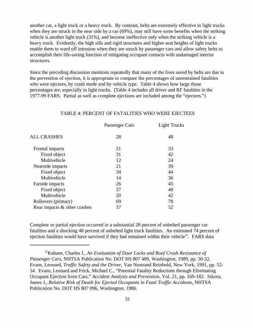
Since the preceding discussion mentions repeatedly that many of the lives saved by belts are due tothe prevention of ejection, it is appropriate to compare the percentages of unrestrained fatalitieswho were ejectees, by crash mode and by vehicle type. Table 4 shows how large thosepercentages are, especially in light trucks. (Table 4 includes all driver and RF fatalities in the1977-99 FARS. Partial as well as complete ejections are included among the “ejectees.”)

TABLE 4: PERCENT OF FATALITIES WHO WERE EJECTEES

Passenger Cars Light Trucks

ALL CRASHES 28 48

Frontal impacts 21 33Fixed object 31 42Multivehicle 12 24

Nearside impacts 21 39Fixed object 34 44Multivehicle 14 36

Farside impacts 26 45Fixed object 37 48Multivehicle 20 42

Rollovers (primary) 69 78Rear impacts & other crashes 37 52

Complete or partial ejection occurred in a substantial 28 percent of unbelted passenger carfatalities and a shocking 48 percent of unbelted light truck fatalities. An estimated 74 percent ofejection fatalities would have survived if they had remained within their vehicle31. FARS data

32In 1977-99 FARS data, the ratio of ejection to nonejection fatalities is 91 percent lowerfor belted occupants than for unbelted occupants of cars equipped with 3-point belts, and also inlight trucks. Even if belts had no effect on non-ejected fatalities, this would imply a 91 percentreduction of the probability of ejection. To the extent that belts also reduce nonejection fatalities,the reduction of the probability of ejection is greater than 91 percent.

32

suggest that 3-point belts reduce the probability of ejection by at least 91 percent in fatal crashes incars and also in light trucks32. If safety belts had no benefits other than preventing ejection, theywould reduce overall fatality risk by

0.28 x 0.74 x 0.91 = 19 percent in passenger carsand

0.48 x 0.74 x 0.91 = 32 percent in light trucks

In other words, prevention of ejection accounts for a substantial portion of the benefit of belts, butnot nearly all the benefits. The overall effectiveness of belts is 45 percent in cars and 60 percent inlight trucks, well beyond the 19 and 32 percent attributable to preventing ejection. Much of theirbenefit comes from mitigating injuries within the vehicle. These statistics also show one of themain reasons why belts are more effective in light trucks than in cars: a lot more of the fatalities inlight trucks are ejectees.

Table 4 also shows substantial differences in the proportions of ejectees by crash mode. Inrollovers, of course, the majority of unbelted fatalities are ejectees from passenger cars (69%), buteven more so from light trucks (78%). Ejectees account for a large proportion of the fatalities in“rear and other” impacts. However, ejection is also quite common in frontal and side impacts withfixed objects, more so than in multivehicle crashes. For example, in frontal impacts of passengercars, 31 percent of the fatalities were ejectees in fixed-object collisions but only 12 percent incollisions with other vehicles. That goes a long way to explaining why belts are more effective infixed-object than in multivehicle frontal collisions (60 vs. 42 percent according to Table 3). Ejectees also account for a larger proportion of the fatalities in farside than in nearside impacts(because a smaller proportion of the farside impacts involve intrusion that endangers theoccupant).

The only crash modes in which fewer than 15 percent of the fatalities are ejectees are multivehiclefrontal and nearside impacts of passenger cars. In the frontals, belts are still quite effective (42%according to Table 3), even though ejection is not a major factor, because they mitigate occupantinjuries within the vehicles. But in the nearside impacts, belts have little effect (5% according toTable 3) because intrusion takes away opportunities for belts to minimize occupant contacts withinterior surfaces.

Another factor that makes belts more effective in light trucks than cars is that a large proportion oflight-truck fatalities are in rollovers, where belts are most effective, as shown in Table 5.

33

TABLE 5: CRASH MODE DISTRIBUTION OF UNRESTRAINED FATALITIES


Frontal impacts 55 52Nearside impacts 19 10Farside impacts 10 7Rollovers (primary) 13 27Rear impacts & other crashes 3 4

100 100

Rollovers account for 27 percent of the fatalities of unrestrained occupants in light trucks, but only13 percent in cars. By contrast, cars are especially vulnerable in nearside impacts, accounting for19 percent of fatalities - where belts are least effective. Only 10 percent of unrestrained light-truckfatalities are nearside.

Tables 2 - 5 demonstrate three reasons why belts are more effective in light trucks than in cars:

C Ejection is substantially more frequent for unbelted occupants of light trucks than cars.C Belts are much more effective in side impacts of light trucks - especially nearside impacts

by light vehicles - because intrusion is much less of a problem in light trucks.C Light trucks have relatively more rollovers, where belts are most effective, and relatively

fewer side impacts, where belts are least effective.

Table 6 aggregates across crash modes to estimate effectiveness for all types of single vehiclecrashes and all multivehicle crashes, the latter subdivided by the type of the “other” vehicle.

TABLE 6: FATALITY REDUCTION - SINGLE VS. MULTIVEHICLE CRASHES



Single vehicle 58 x 49 xx 70 xMultivehicle 32 x 17 xxx 43 x

With a car 41 x 20 xxx 57 xWith a light truck 31 x 15 xxx 45 xxWith a heavy truck 25 xx 19 xxx 28 xx


33Evans, Traffic Safety and the Driver (op. cit.), p. 233. Partyka, Papers on Adult SeatBelts (op. cit.), p. 1-12.

34Since cars with 2- and 3-point belts for outboard occupants both have just a lap belt forthe CF occupant, they were combined for the CF analysis.

34

Effectiveness is substantially higher in single-vehicle crashes (fixed-object impacts + rollovers +other non-collisions) than in multivehicle crashes: 58 vs. 32 percent in cars with 3-point belts, 70vs. 43 percent in light trucks. In multivehicle crashes, belt effectiveness is the highest when the“other” vehicle(s) is a passenger car, and lowest when it is a heavy truck. However, 3-point beltshave point estimates 25 percent or higher in every configuration in Table 6.

Evans and Partyka both observed higher effectiveness of belts for drivers than RF passengers indouble-pair comparisons of pre-1986 FARS data, although Evans’ confidence bounds for the tworeductions substantially overlap33. Table 7 presents estimates of belt effectiveness by seat positionbased on 1986-99 FARS data, including the effect of the lap belt for the center-front (CF)occupant.

TABLE 7: FATALITY REDUCTION BY SEAT POSITION



In All Crashes

Driver 48 x 38 xx 61 xRF passenger 37 x 12 xxx 58 xCF passenger lap belt34 4 xxx 7 38 xxx

In Frontal Crashes

Driver 52 x 34 xx 54 xRF passenger 45 x 14 xxx 48 x


The data continue to show somewhat higher effectiveness for the driver (48%) than the RFpassenger (37%) in cars with 3-point belts. Based on the 1986-99 FARS data alone, thisdifference is statistically significant. In light trucks there is less difference, 61 vs. 58 percent.

35To evaluate belts for the CF passenger, records of MY 1975-99 vehicles with a driverand a CF passenger were extracted from 1986-99 FARS files. Both the driver and the CF had tohave known reported belt use, at least one and perhaps both fatally injured. There were only1,985 cars with a driver and CF, as compared 70,668 cars having a driver and RF. With this smallsample, analyses were limited to basic double-pair comparisons and correction by the UEF, as inSections 4 and 5, with no separate computation and weighting by crash mode. Since cars with 2-and 3-point belts for outboard occupants both have just a lap belt for the CF occupant, they werecombined for the CF analysis.

36Two sets of double-pair comparisons are performed: (1) drivers subdivided by age group(and RF can be any age 14 and over) to compute driver effectiveness by age group; (2) RFsubdivided by age group (drivers any age) to compute RF effectiveness. These estimates werethen weighted by unrestrained fatalities by age group, crash mode and seat position. RF age 5-14were analyzed separately, by double-pair comparison with drivers of any age. When data wereinsufficient to subdivide and average across 8 crash modes, simplified analyses with just 3 crashmodes (frontal, side, rollover + other) or without any subdivision were employed.

35

One reason that driver belt effectiveness could be higher is that unaccompanied drivers are slightlyoverinvolved in rollovers, where belts are especially effective, while a large portion of RF fatalitiesare in right-side impacts, where belts are least effective. For an analysis unbiased by possibledifferences in the distribution of crash modes, the lower half of Table 7 estimates effectiveness infrontal crashes only. Even in frontals, belt effectiveness is consistently higher for drivers than forRF: 52 vs. 45 percent in cars with 3-point belts and 54 vs. 48 percent in light trucks. The resultssuggest that the function of the driver’s belt (protecting the driver from dangerous impact with thesteering assembly) may be even more valuable than the function of the RF belt (protecting the RFfrom dangerous impacts with the instrument panel).

The 1986-99 FARS data do not contain enough cases of belted CF occupants of passenger cars fora statistically meaningful estimate of the overall effectiveness of lap belts (4%), let alone anyanalyses of subsets of the data35. The effectiveness of the CF lap belt in light trucks has a largepoint estimate, 38 percent, but it is highly uncertain.

The effectiveness of safety belts by occupant age, as shown in Table 8, is of interest. Belts couldbe less effective for the youngest and oldest occupants, who are least able to tolerate loading fromthe belt in crashes; young occupants also have difficulty wearing belts correctly.

Table 8 confirms that belts are most effective for occupants 15 to 54 years old, and effectivenessdrops off for pre-teen and early-teen passengers, as well as for occupants over 70 and, especially,over 8036. For example, in passenger cars, the highest estimate is 50 percent fatality reduction atage 15-29, dropping to 34 percent at age 5-9 and 27 percent at age 80 or older. Light trucks havethe same trend.

36

TABLE 8: FATALITY REDUCTION BY OCCUPANT AGE



In All Crashes

5- 9 (passengers) 34 xxx - 10 xxxx 59 xxx10-14 (passengers) 35 xx 12 xxxx 63 xx15-29 50 x 38 xx 63 x30-54 49 x 44 xx 64 x55-69 43 x 26 xxx 53 xx70-79 38 x 17 xxxx 42 xx80 and older 27 xx - 11 xxxx 30 xxx

In Frontal Crashes

5- 9 (passengers) 37 xx - 46 xxxx 45 xxx10-14 (passengers) 48 xx 15 xxxx 61 xxx15-29 52 x 33 xx 54 x30-54 51 x 38 xxx 58 x55-69 44 x 33 xxx 41 xxx70-79 39 xx 2 xxxx 34 xxx80 and older 36 xx 38 xxxx 28 xxx


Still, it is noteworthy how little, rather than how much effectiveness drops off for the youngest andoldest occupants, considering that a 3-point belt is really not designed to fit the 5-9 year old child,and considering the great vulnerability of people over 80 to impact loads. Although safety beltsare not ideal protection for these occupants, they are clearly better than no protection at all.

Moreover, the basic results in the top section of Table 8 overstate the drop-off. Young and oldoccupants are underrepresented in rollover crashes, where belts are especially effective. All of thechildren and most of the oldest occupants are RF passengers - whereas belts are more effective fordrivers. Thus, when the analysis is limited to frontal crashes, as in the lower half of Table 8,effectiveness in passenger cars varies only from 37 percent at age 5-9, to 52 percent at age 15-29,and back to 36 percent at age 80 and older.

37

Similarly Tables 8-D (drivers) and 8-P (passengers) confirm that effectiveness remains fairlyconstant, at each seat position, over a wide range of occupant age. For example, effectiveness forcar drivers in frontal crashes drops gradually from 52 percent for age 15-29 to 40 percent for age80 and above.

TABLE 8-D: DRIVERS - FATALITY REDUCTION BY AGE



In All Crashes

15-29 51 x 40 xx 63 x30-54 49 x 46 xx 64 x55-69 44 x 29 xxx 53 xx70-79 39 xx 25 xxxx 39 xxx80 and older 28 xx - 15 xxxx 28 xxx

In Frontal Crashes

15-29 52 x 33 xx 54 x30-54 51 x 38 xxx 58 x55-69 44 x 33 xxx 41 xxx70-79 40 xx 10 xxxx 32 xxx80 and older 40 xx 41 xxxx 28 xxx


37Evans, Traffic Safety and the Driver (op. cit.), pp. 22-25.

38The procedures are similar to the analyses by occupant age.

38

TABLE 8-P: RF PASSENGERS - FATALITY REDUCTION BY AGE



In All Crashes

5- 9 34 xxx - 10 xxxx 59 xxx10-14 35 xx 12 xxxx 63 xx15-29 49 x 32 xx 63 x30-54 44 x 33 xxx 63 x55-69 39 xx 13 xxx 57 x70-79 35 x - 5 xxxx 52 xx80 and older 27 xx - 2 xxxx 40 xxx

In Frontal Crashes

5- 9 37 xx - 46 xxxx 45 xxx10-14 48 xx 15 xxxx 61 xxx15-29 55 x 34 xx 57 x30-54 50 x 33 xxx 54 x55-69 48 xx 4 xxxx 43 xx70-79 37 xx - 21 xxxx 43 xx80 and older 29 xx 31 xxxx 25 xxx


Belt effectiveness might also differ for male and female occupants. “Real” anatomical orphysiological differences that could influence effectiveness include: greater vulnerability of femalesto impact loads37, belts improperly fitting small occupants (primarily female) or exceptionally largeoccupants (usually male). Furthermore, behavioral differences affect the crash exposure of malesand females, with consequences for the overall effectiveness - e.g., young males are overinvolvedin rollovers, where belts are especially effective; when a male and female ride together, the male ismore often the driver. Table 9 analyzes belt effectiveness by occupant gender38.

39

TABLE 9: FATALITY REDUCTION BY OCCUPANT GENDER



In All Crashes

Male 45 x 34 xx 60 xDriver 46 x 37 xx 60 xRF passenger 44 x 19 xxx 61 x

Female 45 x 33 xx 62 xDriver 51 x 41 xx 66 xRF passenger 33 x 17 xxx 57 x

In Frontal Crashes

Male 49 x 33 xx 53 xDriver 49 x 36 xx 53 xRF passenger 51 x 18 xxx 54 x

Female 52 x 29 xxx 53 xDriver 56 x 33 xxx 59 xRF passenger 43 x 21 xxx 44 x


Overall belt effectiveness is nearly the same for male and female occupants. For example, in allcrashes of passenger cars with 3-point belts, the estimates are identically 45 percent. Estimates arewithin a few percent, or identical, in frontal crashes, and in light trucks. However, Table 9 showsone pattern that is too strong and consistent to dismiss as coincidence: belt effectiveness isconsistently higher for female drivers than RF, whereas among males, belt effectiveness is nearlyequal for drivers and RF. The pattern appears even when the analysis is limited to frontal crashes(e.g., 56 vs. 43 percent for female drivers and RF in passenger cars). In fact, belts appear to bemore effective for the female than the male driver, but less effective for the female than the maleRF. Perhaps, belts are especially effective in protecting the small female, but less so the large male,from harmful contact with the steering assembly - compensating for other disadvantages of thefemale occupant (greater vulnerability to impact, poor belt fit). On the other hand, the observedpattern could be due to an artifact of the data - e.g., female passengers might be the group leastlikely to misreport their belt use, resulting in lower observed effectiveness estimates.

39I.e., MY 1975-79 vehicles involved in fatal crashes during 1986-99.

40This effectiveness estimate is the fatality reduction for safety belt plus air bag relative toair bag alone.

40

One of the most important reasons for analyzing 1986-99 FARS data is to find out if theeffectiveness of 3-point belts has changed since the early 1980's - by computing separate estimatesfor vehicles of older and more recent model-year groups. Modifications that made vehicles safer ingeneral, such as air bags or side impact protection, would not necessarily influence belteffectiveness if they have more or less the same relative benefits for the unrestrained as well as thebelted occupant. On the other hand, specific improvements to belt systems, such as pretensionersor load limiters, could augment belt effectiveness, since they have benefits for the belt user and nobenefits for the unrestrained occupant. Table 10 presents effectiveness estimates for severalgenerations of vehicles, and for specific types of automatic belts.

TABLE 10: FATALITY REDUCTION BY BELT TYPE AND MODEL YEAR GROUP


Fat. Fat.Red. Mser* Red. Mser*

Manual belts in non-air-bag vehicles 45 x 60 xMY 1975-7939 47 x 49 xxMY 1980-85 46 x 63 xMY 1986 + 42 x 60 x

Manual belts in dual-air-bag vehicles40 48 x 63 xx3-point automatic belts 48 xx n/a2-point automatic belts (with or w/o lap belts) 32 xx n/a


The effectiveness of all types of 3-point belts is close to 45 percent in passenger cars. There islittle difference in the manual belts of MY 1975-79 (47%), MY 1980-85 (46%), MY 1986-89(42%) or MY 1990-99 with dual air bags (48%) - these variations are easily within the “noise”range of the sampling error. In other words, when cars were made safer during 1975-99, theybecame safer by about the same relative amount for the belted and the unrestrained occupant.

For light trucks, the MY 1975-79 estimate (49%) is lower than the others (all close to 60%). Thisquite possibly is due to a modest proportion of the MY 1975-79 trucks being equipped withseparate lap and shoulder belts, or even with lap belts only, rather than with integral 3-point belts.

41The 1994 NOPUS controlled-intersection survey is the latest file of belt use observationsplus VINs to allow decoding of the type of belts. The use rates in cars with automatic 3-pointbelts, and in cars [of about the same age] with manual belts and air bags were both 69 percent.

42Evans, Traffic Safety and the Driver (op. cit.), pp. 235-236.

43For MY 1981-98, car weights in this analysis are based on decoding the VINs of theFARS cases to determine make-model/body type and linking to the Polk National VehiclePopulation Profile, which provides accurate curb weights. Prior to MY 1981, we used FARSVIN_WGT plus 100 pounds, since that variable in the past averaged 100 pounds below curbweight. For MY 1999, VIN_WGT has become a good estimate of curb weight.

41

However, it is hard to draw conclusions because the sampling error of the MY 1975-79 estimate isrelatively large (since the N of belted occupants is small in those older trucks).

Observed belt effectiveness in cars of the 1990's with dual air bags is a few percentage pointshigher than in earlier cars. This is not a significant increase, given the sampling errors. However,the numbers are at least consistent with the possibility that recent improvements to belt systems,such as pretensioners and load limiters, could be a factor.

Three-point automatic belts, when used, are about equally effective (48%) as manual belts in cars,when used (45%). The 1994 National Occupant Protection Use Survey shows equal use rates forautomatic and manual 3-point belts41. In other words, the automatic and manual 3-point beltsystems are basically equivalent in effectiveness and benefits (i.e., effectiveness x use).

Earlier studies did not show large differences in belt effectiveness in light and heavy cars42. Table11 estimates belt effectiveness for three curb-weight groups of passenger cars43.

TABLE 11: FATALITY REDUCTION BY PASSENGER CAR WEIGHT

In All Crashes In Frontal Crashes

Fat. Fat.Curb Weight Red. Mser* Red. Mser*

2499 pounds or lighter 48 x 52 x2500-3149 pounds 44 x 52 x3150 pounds or heavier 41 x 45 x


44Table 12 is limited to MY 1985-98 light trucks with decodable VINs.

42

The fatality reductions for all types of crashes show slight decreases as the cars get larger, but thedifferences are in the “noise” range. Belts are perhaps more effective in small cars because theyhave a higher proportion of rollovers. However, Table 11 shows a similar slight trend even infrontal crashes: 52 percent reductions for small and middle-weight cars, and 45 percent in heavycars. In other words, there is no clear evidence of differences by car size. Intuitively, both smalland large cars have characteristics that favor belts. Small cars tend to have younger occupants anda higher proportion of single-vehicle crashes, but large cars offer better protection againstintrusion.

Table 12 estimates belt effectiveness for different types of light trucks44.

TABLE 12: FATALITY REDUCTION BY LIGHT TRUCK TYPE

In All Crashes In Frontal Crashes

Fat. Fat.Red. Mser* Red. Mser*

Pickup truck 58 x 52 xCompact pickup 55 x 43 xxFull-sized pickup 61 x 59 x

Van or SUV 63 x 55 xMinivan 60 x 53 xxFull-sized van 62 xx 45 xxxCompact SUV 67 x 61 xxFull-sized SUV 74 xx 51 xxx


In general, the various types of light trucks have overall effectiveness close to 60 percent andfatality reductions in frontal crashes close to 53 percent (the averages for all light trucks in Tables1 and 2).

There are two hints of divergence from the average. Compact pickup trucks have point estimatesof belt effectiveness lower than average, especially in frontals. Compact SUVs have pointestimates slightly higher than the average. At first glance, it is peculiar that frontal effectiveness is61 percent in compact SUVs but only 43 percent in compact pickups, given that manufacturersoften build similar chassis, frame and body parts into their compact SUVs and pickups. However,the two vehicle types have dissimilar drivers and exposure patterns, resulting in different crashdistributions: SUVs have more rollovers, more off-road excursions, and more ejections. In

45The basic assumptions and procedure were documented by Partyka, Susan C., LivesSaved by Seat Belts from 1983 through 1987, NHTSA Publication No. DOT HS 807 324,Washington, 1988. They were reconfirmed by Blincoe, Lawrence J., Estimating the Benefitsfrom Increased Safety Belt Use, NHTSA Publication No. DOT HS 808 133, Washington, 1994,Appendix A; Klein, Terry M. and Walz, Marie C., Estimating Lives Saved by Restraint Use inPotentially Fatal Crashes, NHTSA Research Note, Washington, 1995.

43

compact SUVs, 65 percent of the unbelted fatalities are complete or partial ejections, the highestfor any truck type, but only 49 percent in compact pickups. In frontal crashes, 47 percent of theSUV fatalities are ejectees, but only 34 percent in the pickups. Even in multivehicle frontalcrashes, 37 percent of the SUV deaths are ejectees, but just 24 percent in the pickups. It isunknown whether the high ejection rate in SUVs represents vehicle factors (e.g., large sidewindows) in addition to exposure factors, but in any case this explains the high effectiveness ofbelts in SUVs.

9. VALIDATION: BELT USE OF FATALITIES VS. OBSERVED ON THE ROAD

History Since 1988, NHTSA has relied on the following assumptions and procedures to estimatethe number of lives saved by safety belts at front-outboard seats each year:

C The belt use of fatally injured occupants on FARS is accurately reported.

C Belt effectiveness is 45 percent in passenger cars and 60 percent in light trucks.

C Thus, for every 55 belted, fatally injured passenger car occupants on FARS, there mustexist 45 other people who were saved by the belt (and these people cannot necessarily beseen on FARS - e.g., if everybody in the crash survived), and for every 40 belted light truckfatalities on FARS there must exist 60 other people who were saved by the belt45.

While developing the procedure, NHTSA staff identified four different use rates for belts:

U1 = the actual use rate of fatally injured occupants as reported (accurately, we believe) onFARS. U1 = F1 / (F0 + F1) where F0 is the number of unrestrained fatalities and F1 is thenumber of belted fatalities.

U2 = the hypothetical belt use in potentially fatal crashes (UPFC), the use rate for the combinedpopulation of fatally injured people plus those who must have been saved by the belt. Ifeffectiveness is E,

U2 = {F1 + [E x F1 / (1-E)]} / {F0 + F1 + [E x F1 / (1-E)]}

In other words, we add [E x F1 / (1-E)], the hypothetical number of people who were savedby the belt, to both the numerator and the denominator of U1.

46Reinfurt, Donald W., Silva, Claudio Z. and Seila, Andrew F., A Statistical Analysis ofSeat Belt Effectiveness in 1973-75 Model Cars Involved in Towaway Crashes, Volume 1,NHTSA Publication No. DOT HS 802 035, Washington, 1976, pp. v-x and 13. Final RegulatoryImpact Analysis, Amendment to Federal Motor Vehicle Safety Standard 208, Passenger CarFront Seat Occupant Protection, NHTSA Publication No. DOT HS 806 572, Washington, 1984,p. IV-6.

44

U3 = the actual belt use observed on the road for the general traffic population in state surveys,the National Occupant Protection Use Survey (NOPUS), or the 19-City Study.

U4 = the reported belt use of crash survivors on FARS. This number is not consideredmeaningful, at least in absolute terms, because crash survivors have been overreportingtheir belt use since 1986, when belt use laws took effect in most of the large states (seeSections 1 and 4). It is further bloated by cases of occupants saved by the belt who gotinto the FARS system because some other person was killed in the crash.

U1, U2, and U3 are meaningful numbers. The relationship between them was studied extensively atNHTSA. Specifically, U1 is less than U2, by definition, whereas U2 for the overall potentially-fatal-crash population is empirically demonstrated to be less than U3 for the general motoring public.

U1 is less than U2 because belt use of fatally injured occupants excludes the belt users who weresaved by the belt, while UPFC includes them. The relationship between the actual rate U1 and thehypothetical rate U2 is deterministic, not statistical, and it can be specified exactly wheneffectiveness E is known. Indeed, U2 is a hypothetical rate that cannot be observed, but can onlybe imputed from U1 and E by the following formula:

U2 = U1 / {1 - [E x (1 -U1)]}

Conversely, U1 = [(1 - E) x U2] / [1 - (E x U2)]

For example, if U1 is 50 percent and E is 45 percent then U2 is necessarily 64.52 percent.

U2 is less than U3 because the type of people who get involved in actually or potentially fatalcrashes are less likely to use belts than the average person observed in seat belt surveys. It haslong been known that belt users are, on the average, more cautious drivers than non-users, andunderinvolved in severe crashes46. Alcohol-impaired drivers, risk-takers and people oblivious tosafety are less likely to use belts and they are overinvolved in severe crashes. Another factor isthat observational surveys are usually during the daytime, when belt use is higher, while many fatalcrashes are at night.

However, the relationship of U3 to U2 is not deterministic but can vary over time and place. Theonly certainties are when U3 is 0 percent, so is U2 and when U3 is 100 percent, so is U2. At all

47Partyka, Susan C. and Womble, Kathleen B., Projected Lives Savings from Greater BeltUse, NHTSA Research Note, Washington, 1989. Blincoe (op. cit.), Appendix B.

45

intermediate points, U2 lags behind U3. NHTSA uses empirical statistical models47 such asquadratic regressions over time and across states to model the “typical” lag of U2 behind U3. These models are needed to achieve two program objectives: (1) Predicting how many additionallives would be saved if on-the-road belt use increased by a specified number of percentage points;(2) Conversely, estimating U3 for states that did not perform observational surveys that year, basedon U1 observed and U2 calculated from FARS data for that year.

There are always two known, observable quantities U1 and U3 and two hypothetical constructs thatcannot be directly observed, E and U2. All of the above procedures simply assumed E was alsoknown (45 percent in cars and 60 percent in light trucks) and used the three “knowns” U1, U3 andE to calculate the other unobservable quantity U2 as well as the important statistic U3 - U2.

Analysis overview In the remainder of this report, the process will be reversed: we will assumewe know U2, the UPFC, and use it with U1, the belt use of fatally injured occupants to estimate theeffectiveness E. Just as in Sections 3-8, though, these point estimates, relying on several criticalassumptions, are not like customary statistical estimates derived directly from the data. Theiruncertainty can be discussed to some extent, but not be fully quantified, based on statistical theory,with “confidence bounds.” The analysis is another empirical tool to support a qualitativejudgement if NHTSA’s long-standing estimates of 45 percent fatality reduction in cars and 60percent in light trucks are still appropriate.

The above formulas for U1 or U2 can be solved for E:

E = [U2 - U1] / [U2 - (U2 x U1)]

Specifically, we will identify a subset of occupants in potentially fatal crashes whose belt use isarguably the same as the average road-users included in observational surveys - i.e., U2 = U3

for this subset. Then we can substitute the known, observed U3 for the unobservable U2 in thepreceding formula, and together with the belt use U1 of the fatalities in that subset, estimate theeffectiveness:

E = [U3 - U1] / [U3 - (U3 x U1)]

For example, if 50 percent of the fatalities were belted in this special subset, and belt use on theroad were 65 percent, belt effectiveness would be 46.15 percent.

In 1989, Susan Partyka took the first step in the direction of this analysis when she computed U1

and U2 for various subgroups in 1987-88 FARS - still assuming E = 45 percent in deriving U2 fromU1 - and then compared them to U3 = 44 percent, the observed belt use in passenger cars during

48Partyka, Susan C., Belt Use in Serious Impacts Estimated from Fatality Data, NHTSAPublication No. DOT HS 807 519, Washington, 1989. Bowman, Brian L. and Rounds, DonaldA., Restraint System Usage in the Traffic Population - 1988 Annual Report, NHTSA PublicationNo. DOT HS 807 447, Washington, 1989.

46

1987-88 in 19 U.S. cities48. Although U2 for the entire FARS was well below 44 percent, U2 fordrivers without police-reported alcohol use was 46 percent and U2 for drivers in daytime, weekdaycrashes, without police-reported alcohol use or previous crash involvements was 51.5 percent,actually exceeding belt use observed in the 19 cities. This study confirmed that the agency’s 45percent effectiveness estimate was more plausible than higher numbers proposed by someresearchers. It also demonstrated some groups had lower-than-average belt use: alcohol-impaireddrivers, people with bad driving records, and nighttime traffic.

The analysis in this report will be based on 1991-99 FARS, a large data base. Belt use of fatallyinjured occupants will be compared to belt use on the road, derived from national averages of1991-99 state observational surveys. We will define a FARS subgroup that arguably ought tohave UPFC equal to observed belt use on the road: non-drinking, “non-antisocial,” daytimeinvolvements in multivehicle crashes [or, alternatively, non-drinking, “non-antisocial,” daytimeinvolvements in all crashes]. This group can be defined on a fairly consistent basis across the statesand avoids some biases inherent in FARS data, as will be explained later. U1 will be obtained fromFARS for passenger cars with 3-point belts and for light trucks. The heart of the analysis is anadjustment of the 1991-99 state belt use rates, with the help of NOPUS and other data, to obtainseparate U3 rates for cars with 3-point belts and for light trucks that are comparable to U1. Finally,U1 and U3 will be used to compute the effectiveness E - but with a recognition that effectiveness inthis special subset of crashes (e.g., limited to multivehicle) should not necessarily be the same asfor all crashes.

Issues that must be considered in making state survey results comparable to FARS are:

C State surveys generate a single use rate each year, aggregating cars with 3-point belts, carswith 2-point automatic belts, and light trucks. We need to tease out separate rates for carswith 3-point belts and for light trucks, based on differentials seen in other data.

C Before 1998, a fair number of state surveys omitted some or all light trucks if the law inthat state did not cover light trucks and/or for other reasons. Many surveys omitted localroads, and a few were limited to drivers. Results need to be adjusted to reflect all front-outboard occupants of all types of light vehicles on all roads.

C Observational surveys have a rural-urban mix proportional to VMT, but FARS cases haveproportionately more rural crashes.

49Klein, Terry M., A Method for Estimating Posterior BAC Distributions for PersonsInvolved in Fatal Traffic Accidents, NHTSA Publication No. DOT HS 807 094, Washington,1986.

47

FARS data analysis A basic working assumption here, as elsewhere in this report and otherNHTSA studies, is that the belt use of fatally injured occupants is reported accurately in FARS, orat least without a net bias (net over- or underreporting).

Another given is that we cannot prove with existing data that any specific subgroup of peopleinvolved in fatal or potentially fatal impacts actually has the same belt use as the average person onthe road. The people “saved by the belt,” who are a part of the subgroup, simply aren’t in thedata. We can only make a logical argument, supported by the literature, that this subgroup oughtto have the same belt use as the general population.

This is fundamentally a process of excluding groups with behaviors that are typically associatedwith lower-than-average belt use, leaving a kernel of people “just like you and me” who had themisfortune of becoming involved in a fatal crash. The process needs to be reasonably consistentacross states and from year to year (1991-99).

As noted above, an excellent starting point is to exclude alcohol-impiared drivers and theiraccompanying RF passengers. However, the completeness of FARS/police reporting of alcoholinvolvement varies a lot from state to state49. Nineteen states, including California, Texas, Floridaand Illinois have “not reported,” “unknown” or missing data on over 40 percent of driver fatalitiesin cars or light trucks during 1991-99. Moreover, in some states (such as Texas and Missouri)these codes are often a surrogate for “no alcohol” while in others they really mean “unknown.”

That raises a question of whether to include only those specifically reported as “no alcohol” (andexclude the unknowns) or merely to exclude those positively reported as “alcohol-involved” (andinclude the unknowns). Limiting to the “no alcohol” cases is unsatisfactory because it woulddelete almost all the Texas and Missouri data and over 70 percent of California, Illinois, Georgia,Wisconsin, etc. cases: what remains would not be nationally representative. On the other hand,excluding only the “alcohol-involved” cases and retaining the unknowns would leave a fair numberof drinking drivers in the file: 17 states, including New York, Florida, North Carolina and Georgia,list under 20 percent of their cases as positively alcohol-involved (hard to believe - except Utah).

Thus, it is appropriate to exclude all driver records, and their accompanying RF passengers, thatwere positively coded as “alcohol-involved,” but that is only a starting point. We must identifyother behaviors that should be excluded, and that will make the exclusion rate more uniform acrossstates.

A more sweeping approach that turns out to be unsuccessful is to rely on the widely-acceptedtheory of “induced exposure”: the non-culpable party(s) in a multivehicle crash is for all practical

50Haight, Frank A., Indirect Methods for Measruing Exposure Factors as Related to theIncidence of Motor Vehicle Traffic Accidents, NHTSA Publication No. DOT HS 800 601,Washington, 1971. Cerrelli, Ezio, Driver Exposure: Indirect Approach for Obtaining RelativeMeasures, NHTSA Publication No. DOT HS 820 179, Washington, 1972.

48

purposes a typical road user who just happened to be in the wrong place at the wrong time50. Thatseems exactly what we need, even if it limits us to certain multivehicle involvements, because wecan be confident this group will have UPFC equal to the belt use of typical road users.

The FARS variables, “Related Factors - Driver Level,” DR_CF1 - DR_CF4 identify culpabledrivers to be excluded: anybody with one or more of these variables equal to 6, 26, 27, 28, 30, 31,35, 36, 38, 39, 44, 48, 50, 51, 57 or 58. Most of these codes are specific, momentary drivingerrors that lead directly to collisions: lane departure, failure to obey traffic signal, failure to yieldright of way, driving too fast for conditions, following too closely, etc. They are generally notunderlying behavioral problems or long-term conditions (although the culpable drivers may havesome of those, too). The non-culpable drivers to be included in the analysis are a large group withno DR_CF codes at all, and a smaller group with other codes than the above, generally notpertaining to specific driving errors (e.g., glare, crosswind).

Unfortunately this approach does not work with FARS data, even though it has been quitesuccessful with primarily nonfatal state data. The DR_CF codes in FARS are severely confoundedwith whether or not the driver survived. A disproportionate share of the driving errors areattributed to the fatally injured driver in a multivehicle crash. This becomes clear, for example, inhead-on, front-to-front collisions of two vehicles. Intuitively, which driver dies and which survivesought to have a lot to do with the relative weights of the vehicles and ages of the drivers, and littleto do with who “started” the collision by crossing the center-line. Head-on is pretty much head-on, regardless of how or where it happened. But in FARS, based on the DR_CF codes, 65 percentof the fatally injured drivers in these collisions were culpable, but only 32 percent of the survivingdrivers. There is a strong tendency to blame the crash on the dead driver, and it persists evenwhen the cases are subdivided by driver age, vehicle type, etc. We certainly would not want toanalyze belt effectiveness in a group whose selection factor (culpable or non-culpable) is highlyconfounded with the principal outcome variable of our analysis (survival or non-survival).

The remedy is to find an intermediate approach that works with FARS data. We need to exclude awider range of antisocial behaviors than just the drinking driver, but not exclude all culpabledrivers. The exclusions should be reasonably consistent across states (unlike the FARS alcohol-involvement variable), and not confounded with crash survival (unlike DR_CF as treated above).

The following drivers are excluded from the analysis because they display forms of antisocialbehavior that could indicate a lower belt use rate than the average driver on the road. RFpassengers are excluded if their accompanying driver exhibits any of these behaviors:

49

C FARS positively reports alcohol involvement (DRINKING = 1)C FARS positively reports drug use (DRUGS = 1)C Driving without a license, or with a suspended, revoked, expired, canceled or denied

license (L_STATUS = 0, 1, 2, 3, 4 in 1991-99)C A sub-par driving record as indicated by any one (or more) of the following during the 3

years preceding the fatal crash involvement:S at least 1 DWI conviction, orS at least 2 speeding convictions, orS at least 2 other harmful-moving-violation convictions, orS at least 2 license suspensions or revocations, orS at least 2 police-reported crash involvements

C Possibly antisocial behavior(s) at the time of the crash, as evidenced by any of DR_CF1 -DR_CF4 having the following values:19 driving on suspended or revoked license36 erratic, reckless, careless or negligent driving37 attempting to escape police pursuit46 racing90 hit and run91 vehicular homicide

Since Florida, Kansas, North Carolina, Ohio and Utah encode “erratic, reckless, careless ornegligent driving” far more often than other states, cases will be excluded from these states ifDR_CF1 = 36, but DR_CF2, DR_CF3 or DR_CF4 = 36 will not be grounds for exclusion.

All other drivers, and their accompanying RF passengers will be considered non-antisocial andbecome candidates for inclusion in the study. Inattentive driving due to a temporary distractionsuch as talking or eating (DR_CF = 6) is not considered “antisocial behavior” in this analysis.

The proportion excluded is fairly consistent from state to state, ranging from 15 percent of RhodeIsland daytime driver fatalities in 1994-99 to 45 percent of Kansas fatalities; however 41 of the 51states plus D.C. are in a relatively narrow range of 21 to 34 percent excluded. What remains afterthe exclusions is nationally representative. This is a better filter than the DRINKING variablealone, which resulted in near-zero exclusions from some important states. It is even moreconsistent year-to-year, showing a gradual downward trend from 51 percent excluded in 1977, to45 percent in 1991, to 41 percent in 1999, consistent with the real reductions in alcohol-impaireddriving and some other antisocial driving behaviors in the United States during the past 25 years.

Unlike “culpability,” FARS just minimally confounds this variable with the probability of survivinga crash. In head-on, front-to-front collisions of two vehicles of any type, 33 percent of the fatallyinjured drivers were excluded, but only 28 percent of the surviving drivers. In passenger cars,these percentages are an even closer 33 and 31, respectively.

Most important, it is plausible that the remaining “non-antisocial” drivers and their accompanyingRF passengers buckle up as much as the average road user. A wide range of habitual risk-taking,

50

aggressive or safety-indifferent behaviors - likely to be associated with a low rate of belt use - hasbeen excluded. Although the “non-antisocial” group still includes a fair number of “culpable”drivers, these are mostly one-time, specific driving errors, without a history of previous errors. Although they were “culpable” on that occasion, they are still “average” road users - not perfectdrivers, but susceptible to human error from time to time. Mere “culpability” need not indicatelow belt use.

Since belt use surveys are conducted in the daytime, the analysis is further limited to daytimecrashes, specifically from 7:00 A.M. to 6:59 P.M.

A question arises whether to include single-vehicle crashes. If running off the road per sedemonstrates aggressive, risk-taking behavior, it would be appropriate to limit the analysis tomultivehicle daytime non-antisocial crash involvements. But if running off the road, in the absenceof specific antisocial behaviors, is merely one of the errors occasionally committed by the averagedriver, it would not be necessary to exclude single vehicle crashes. Both approaches will be usedhere.

The 1991-99 FARS data included the following N’s of front-outboard fatalities in daytime, non-antisocial crash involvements, with belt use reported as either yes (REST_USE = 1, 2, 3, 8, 13) orno (REST_USE = 0), in model year 1975-99 passenger cars and light trucks equipped with 3-pointbelts:

C 37,713 multivehicle fatalities in passenger cars (57.5 percent belted)C 11,845 multivehicle fatalities in light trucks (42.3 percent belted)C 49,612 single + multivehicle fatalities in passenger cars (53.1 percent belted)C 19,997 single + multivehicle fatalities in light trucks (36.6 percent belted)

These are large N’s and they enable precise calculation of U1, the belt use rate of fatally injuredoccupants (sampling error based on 1.96 /pq/n is less than 1 percentage point in each case). Thenext tasks are to obtain U3, belt use observed on the road, that we assert equals U2, belt use inpotentially fatal crashes, and compute E, the fatality reducing effectiveness of belts. But first let ustake a step back and use double-pair comparison to estimate what kind of effectiveness we mightexpect to see in daytime, non-antisocial crash involvements.

Anticipated effectiveness, based on double-pair comparison Many rollovers occur at nightand/or involve drivers classified as “antisocial.” Table 2 showed belts are especially effective inrollovers. Thus, we cannot expect safety belts to be as effective in daytime, non-antisocial crashesas they are overall (45 percent in passenger cars, 60 percent in light trucks). Table 6 showed evenlower effectiveness in multivehicle crashes, where almost all rollovers are excluded. Table 13estimates belt effectiveness in daytime, non-antisocial crash involvements, based on the methods ofSections 3-8: double-pair comparison of 1986-99 FARS data, corrected by the UEF.

51Mser = minimum sampling error range (± 1.96 standard deviations) based on the formulain Section 7; does not include possible non-sampling errors from assuming the UEF is applicablefor all collision types, etc.

51

TABLE 13: FATALITY REDUCTION IN DAYTIME, NON-ANTISOCIAL CRASHINVOLVEMENTS - BASED ON DOUBLE-PAIR COMPARISON OF 1986-99 FARS


Fat. Fat.Red. Mser51 Red. Mser

In MULTIVEHICLE daytimenon-antisocial crash involvements 29 ± 10 42 ± 12

In ALL daytimenon-antisocial crash involvements 38 ± 8 52 ± 8

The point estimate of effectiveness for passenger cars in daytime, non-antisocial multivehiclecrashes is just 29 percent, with minimum sampling error range ± 10 percentage points. In otherwords, if the analysis method of this section produced an E anywhere from 19 to 39 percent itwould still be statistically consistent with the double-pair comparison result, and a validation of themethod of Sections 3-8, but the closer it is to 29 percent, the better. Similarly, we wouldanticipate a still-low 38 percent fatality reduction when single-vehicle crashes are included forpassenger cars. For light trucks, the anticipated effectiveness levels are 42 and 52 percent, alsolower than the overall 60 percent fatality reduction in light trucks.

Based on the formula:

U3 = U2 = U1 / {1 - [E x (1 -U1)]}

the belt-use rate of 57.5 percent for fatally injured occupants of passenger cars in the multivehiclecrashes, and the 29 percent effectiveness suggest an anticipated 65.6 percent belt use on the roadin cars during 1991-99. The belt-use rate of 53.1 percent in cars for single + multivehicle fatalities,combined with 38 percent effectiveness anticipate a quite similar 64.6 percent belt use on the road. The anticipated belt-use rates on the road for light trucks, calculated the same way, are 55.8percent and 54.6 percent, respectively. As a first cut, we can see these numbers are reasonablyclose to belt use actually observed on the road during the 1990's, and suggest the remaininganalyses are likely to validate the double-pair comparison estimates. Now, let us proceed withadjusting and interpreting the state observational survey data, so we may calculate a real E from areal U3 rather than an anticipated U3 from an anticipated E.

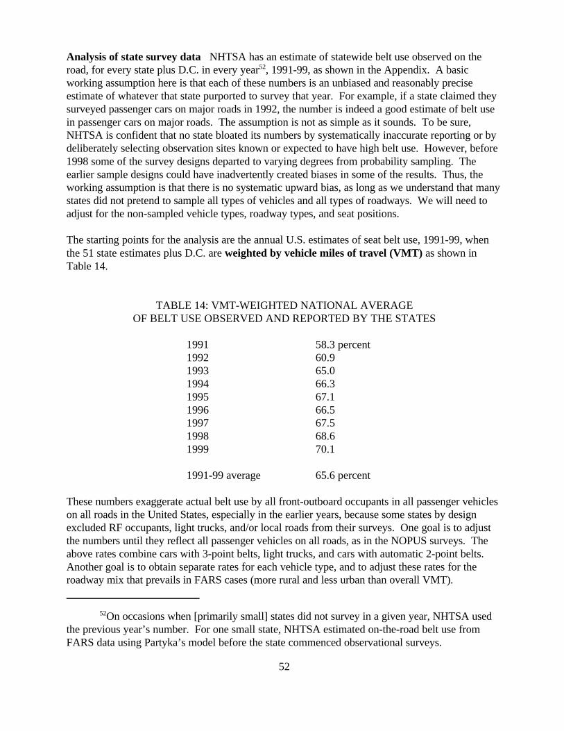
52On occasions when [primarily small] states did not survey in a given year, NHTSA usedthe previous year’s number. For one small state, NHTSA estimated on-the-road belt use fromFARS data using Partyka’s model before the state commenced observational surveys.

52

Analysis of state survey data NHTSA has an estimate of statewide belt use observed on theroad, for every state plus D.C. in every year52, 1991-99, as shown in the Appendix. A basicworking assumption here is that each of these numbers is an unbiased and reasonably preciseestimate of whatever that state purported to survey that year. For example, if a state claimed theysurveyed passenger cars on major roads in 1992, the number is indeed a good estimate of belt usein passenger cars on major roads. The assumption is not as simple as it sounds. To be sure,NHTSA is confident that no state bloated its numbers by systematically inaccurate reporting or bydeliberately selecting observation sites known or expected to have high belt use. However, before1998 some of the survey designs departed to varying degrees from probability sampling. Theearlier sample designs could have inadvertently created biases in some of the results. Thus, theworking assumption is that there is no systematic upward bias, as long as we understand that manystates did not pretend to sample all types of vehicles and all types of roadways. We will need toadjust for the non-sampled vehicle types, roadway types, and seat positions.

The starting points for the analysis are the annual U.S. estimates of seat belt use, 1991-99, whenthe 51 state estimates plus D.C. are weighted by vehicle miles of travel (VMT) as shown inTable 14.

TABLE 14: VMT-WEIGHTED NATIONAL AVERAGEOF BELT USE OBSERVED AND REPORTED BY THE STATES

1991 58.3 percent1992 60.91993 65.01994 66.31995 67.11996 66.51997 67.51998 68.61999 70.1

1991-99 average 65.6 percent

These numbers exaggerate actual belt use by all front-outboard occupants in all passenger vehicleson all roads in the United States, especially in the earlier years, because some states by designexcluded RF occupants, light trucks, and/or local roads from their surveys. One goal is to adjustthe numbers until they reflect all passenger vehicles on all roads, as in the NOPUS surveys. Theabove rates combine cars with 3-point belts, light trucks, and cars with automatic 2-point belts. Another goal is to obtain separate rates for each vehicle type, and to adjust these rates for theroadway mix that prevails in FARS cases (more rural and less urban than overall VMT).

53

Belt use parameters The strategy is to disaggregate national belt use and model it as a primarilylinear function of five discrete variables: vehicle type, belt law, road type, seat position andcalendar year:

4 vehicle typescars with 3-point beltscars with 2-point beltspickup trucksvans/SUVs

2 belt law conditions (depending on vehicle type)covered by lawnot covered by law

4 road typesmajor rural (interstate + arterial)local rural (local + collector)major urban (interstate +freeway + arterial)local urban (local + collector)

2 seat positionsdriverright front (RF)

9 calendar years: 1991 through 1999

Thus, BELTUSE(vehicle, law, road, seat, CY) will be estimated for the United States for a total of4x2x4x2x9 = 576 conditions. We will try to make this a linear model without interaction terms. In other words, if the driver has belt use 4 percentage points higher than the RF passenger inpickup trucks with a belt law on major rural roads in 1991 that will also be true in vans/SUVswithout a belt law on local urban roads in 1992, etc. (The only exception to this independentlinear approach, as we shall see, will be in cars with automatic 2-point belts.) It is necessary toseparate pickup trucks and vans/SUVs in the model, because they have different belt use rates andlaws, but later they will be combined into a single “light truck” estimate.

The parameters for this model will now be derived from various sources, including NOPUS, thestate surveys themselves, and sometimes, survivor belt use on FARS (percentage point differencesbetween rates, not absolute rates).

The effect of seat position is the easiest to derive, since all three full NOPUSes (1994, 1996 and1998) observed and reported belt use separately for drivers and RF. The average belt use in thosethree surveys was 4.0 percentage points higher for the driver than the RF.

53Evaluation of the Effectiveness of Occupant Protection - Federal Motor Vehicle SafetyStandard 208 - Interim Report, June 1992, NHTSA Publication No. DOT HS 807 843,Washington, 1992, p. 13, weighting the three types of 2-point belts in Table 2-2 at 45:40:15.

54Belt use rates among FARS survivors of daytime non-antisocial multivehicleinvolvements show similar differentials - viz., a 9 percentage point decrement for pickups and a 1percentage point increment for vans/SUVs over passenger cars with 3-point belts in 1998.

55The 1996 NOPUS also estimates belt use separately for “major” and “local” roads in“rural” and “non-rural” areas. It, too, shows highest belt use on “major non-rural” roads (67.1%)and lowest on “local rural” roads (57.4%). However, it is preferable to rely on the road-typedefinitions and belt-use differentials of FARS survivors, since they obviously correspond exactlyto categories that are defined for the FARS fatalities, and also to FHWA Highway Statistics.

54

Belt use in any type of vehicle, except cars with automatic 2-point belts, is 24.3 percentage pointslower if there is no belt law than if there is a belt law. This estimate is based on state surveys forCY 1991-94, comparing average belt use in states with laws to use in states without laws, in eachcalendar year.

Now, let us tackle the issue of belt use in cars with automatic 2-point belts, since this informationwill be needed for some of the other parameter estimates. Unlike all other vehicle types, belt use incars with automatic 2-point belts did not change throughout 1991-99, as evidenced by use rates ofFARS survivors. (Although these use rates are not credible as absolute numbers, they can betrusted as evidence that belt use did not change from year to year.) It is also unaffected by beltlaws. The absolute use rate for drivers was a more-or-less constant 84 percent during 1991-99(higher than the national-average use of 3-point belts in any vehicle type, road type or year). Thisis the average of 78.2 percent observed in the 1994 NOPUS (controlled intersections, cars withdecodable VINs) and the 89.5 percent observed in 19 cities during 1990-9153. Given 84 percentuse by drivers, that implies 80 percent for RF passengers (and 83 percent for a 75:25 driver:RFmix) in each CY, on all roads, with or without a belt law

All else being equal, belt use in pickup trucks is 10.8 percentage points lower than in cars with3-point belts. In vans/SUVs it is 0.6 percentage points higher than in cars with 3-point belts. Thedifferentials are estimated from the 1998 NOPUS, as follows. Belt use in all passenger cars is 71.3percent in 1998 NOPUS. Since 13.2 percent of passenger cars in 1998 had 2-point belts (seebelow), used by 83 percent of front-seat occupants, the use rate in cars with 3-point belts wouldhave to be 69.5 percent to get a 71.3 percent average for all cars. That compares to 58.7 inpickups (10.8 percentage points lower than 69.5) and 70.1 in vans/SUVs (0.6 percentage pointshigher)54.

The highest belt use rate is on major urban roads. The percentage point decrements in belt use onother roadway types are: 3.6 on major rural, 10.9 on local rural, 2.7 on local urban, as seen in thereported belt use of survivors in daytime non-antisocial multivehicle involvements. Thesedecrements are for passenger cars with 3-point belts, but are also approximately right for pickuptrucks, vans and SUVs55. Cars with automatic 2-point belts had similar belt use on all roadways.

55

Finally, belt use could change (generally increase) from year to year during 1991-99 (except in carswith automatic 2-point belts). However, the increments cannot be estimated at this point. Thatwill be the final step in developing the model, and it will be derived from the state survey data,after they have been adjusted to create NOPUS-like estimates.

Weight factors Now that we have deconstructed belt use into 576 cells, with a use rate in eachcell, we may reconstruct national overall use rates by assigning a weight factor to each cell andtaking the weighted average. Three sets of weight factors will be defined, allowing three types ofnational estimates:

C A national factor, NATLWGT(vehicle, law, road, seat, CY) that simply weights each cell ina given calendar year according to its proportion of the nation’s VMT in that year (or,more correctly, its proportion of front-outboard occupant miles of travel). When all thecells are weighted by NATLWGT, the result should be a “true” estimate of national beltuse in each year, comparable (but not necessarily equal) to what NOPUS generated in1994, 1996 and 1998.

C A state factor, STATEWGT that equals NATLWGT on those cells where all 51 state +D.C. surveys observe belt use - e.g., passenger car drivers on major roads - but is lowerthan NATLWGT on those cells where some of the states did not observe belt use - e.g.,pickup truck passengers, on local roads, in 1991. Each state is weighted by its share ofVMT; STATEWGT/NATLWGT equals the share of VMT for the states that did surveybelt use in that cell divided by the VMT for all states plus D.C. We will then set the CYparameters for BELTUSE so that when all the cells are weighted by STATEWGT, theresults will exactly equal the annual VMT-weighted national averages of belt use observedand reported by the states, as shown in Table 14. In other words, the basic state estimatesin Table 14 drive the rest of the model.

C A FARS factor, FARSWGT that weights each cell according to its proportion of thenation’s fatalities rather than VMT. We will generate one set of FARSWGT formultivehicle daytime non-antisocial involvements, and another for single + multivehicledaytime non-antisocial involvements. When all the cells are weighted by one of theseFARSWGT, the result will be an estimate of belt use in potentially fatal crashes (UPFC) weneed to complete our analysis.

NATLWGT The procedure for obtaining NATLWGT has two guidelines: (1) Whenever possible,it should use a simple multiplicative model, p(A and B) = p(A) x p(B), with interaction terms(conditional probabilities) only when they are really needed. We will obtain weight factors foreach of the parameters (vehicle type, law, road type, seat position) separately, or two-at-a-time,and multiply them to obtain the cell weight. (2) The cell weights in each CY add up to 1.

56In the 1994, 1996 and 1998 NOPUS, the average ratio was 73 to 27.

57Based on the “Key Provisions of Safety Belt Use Laws” tables in Fatal AccidentReporting System 1991 and Traffic Safety Facts 1992 through Traffic Safety Facts 1998,NHTSA publications. The information is summarized in the Appendix of this report.

58The 1994 NOPUS belt use results, 62.8 percent in cars and 50.2 percent in light trucks,for an overall average of 58.0 percent, imply that 62 percent of the vehicles in the sample werecars and 38 percent were light trucks.

56

The weight factors for seat position are 0.75 for the driver and 0.25 for the RF passenger. The 3to 1 ratio of drivers to passengers has been consistently observed in numerous data bases overmany years56.

Belt laws in many states always applied to all passenger vehicles, but before 1998 there were a fairnumber of states that exempted all light trucks, or just pickup trucks, from the laws. Thepercentages of vehicles in the United States covered by state belt laws (i.e., weighting the states byVMT), by calendar year, are shown in Table 1557. In other words, the “belt law” weight factor forpassenger cars in 1991 is 0.91 and the “no belt law” weight factor is 0.09.

TABLE 15: PERCENT OF VEHICLES COVERED BY BELT LAWS

Passenger Pickup Vans &Cars Trucks SUVs

1991 91.0 64.6 78.11992 93.1 65.2 78.61993 93.7 69.1 79.31994 97.7 73.4 83.61995 99.0 74.7 84.91996 99.6 78.9 85.41997 99.6 78.9 85.41998 & 99 99.6 99.6 99.6

The ratio of passenger cars to light trucks in NOPUS (weighted, moving-traffic data) should be thesame as their ratio of VMT. In 1994, the NOPUS data were 62 percent cars and 38 percent lighttrucks58. Comparable numbers for the 1996 and 1998 NOPUS are 58 percent and 57 percent cars,respectively. Smoothing out this trend gives approximately 64 percent cars in 1991, and thendeclining by 1 percentage point each year, down to 56 percent cars in 1999. Light trucks’ share ofVMT increased 1 percentage point a year from 36 percent in 1991 to 44 percent in 1999.

The passenger car VMT may be subdivided into cars equipped with 3-point belts or with automatic2-point belts, based on the distribution of FARS survivors in daytime non-antisocial multivehicle

59Teets, Mary K., Highway Statistics 1993, Publication No. FHWA-PL-94-023, FederalHighway Administration, Washington, 1994, p. V-116. By FHWA’s definition, a road is either“rural” or “urban”; most roads in suburbs are classified as “urban.”

57

crash involvements, by calendar year. The light truck VMT is split into pickup trucks orvans/SUVs, based on registration data from the R.L. Polk National Vehicle Population Profile. TheVMT shares for the four vehicle types are shown in Table 16. Above all, vans and SUVs increasedat the expense of passenger cars. Pickup trucks remained constant. Two-point automatic beltsincreased at first but began phasing out after 1994 because no new ones were entering the fleet.

TABLE 16: SHARES OF THE NATION’S VMT

Cars, Cars, Pickup Vans &3-Pt. Belts 2-Pt. Belts Trucks SUVs

1991 58.4 5.6 22.4 13.61992 56.5 6.5 22.3 14.71993 54.3 7.7 22.3 15.71994 52.6 8.4 22.8 16.21995 51.8 8.2 22.8 17.21996 50.9 8.1 22.7 18.31997 50.1 7.9 22.7 19.31998 49.5 7.5 22.6 20.41999 49.2 6.8 22.4 21.6

The Federal Highway Administration (FHWA) collects annual statistics on VMT by roadwaysystem. In 1993 (and these distributions change little from year to year), the VMT shares were59:

24.3% major rural (interstate + arterial)14.4% local rural (local + collector)47.4% major urban (interstate +freeway + arterial)13.9% local urban (local + collector)

The FHWA does not count VMT separately by vehicle type. We will use the above distributionfor all vehicle types. Intuitively, light trucks should have proportionately somewhat more ruralVMT and cars more urban. However, FARS data on crash survivors suggests the differences arerelatively small.

NATLWGT is the product of the parameters defined above. For example, the proportion ofoccupant miles traveled in 1991 that were drivers of passenger cars equipped with 3-point belts, instates with belt laws for cars, on major rural roads is:

0.75 x 0.91 x 0.584 x 0.243 = 0.0968549

58

For RF passengers of pickup trucks in states without belt laws on local rural roads in 1996, it is:

0.25 x 0.211 x 0.227 x 0.144 = 0.0017242

STATEWGT is computed for any cell by multiplying NATLWGT by the VMT-weightedproportion of state surveys that included the cell. We will obtain survey-inclusion factors for eachof the parameters (vehicle type, law, road type, seat position) separately, or two-at-a-time, andmultiply them to obtain the cell inclusion factor.

D.C., Kentucky, Missouri and West Virginia, comprising 5 percent of the nation’s VMT, surveyedonly drivers in 1996-97. All other states in 1996-97, and all states in 1998-99 surveyed drivers andRF passengers. In 1994, it is known that six states (or 5 states plus D.C.) surveyed only drivers,but it is unknown which ones. Let us assume those six jurisdictions included D.C., Kentucky,Missouri and West Virginia, and comprised 7.5 percent (5 x 6 / 4) of the nation’s VMT. Let usassume that the coverage in 1991-93 was the same as in 1994, but in 1995 it was midway between1994 and 1996 - i.e., 6.3 percent of the surveys were limited to drivers. In other words, the surveyinclusion parameter for drivers is always 1.0. For RF passengers, it is 0.925 in 1991-94, 0.937 in1995, 0.95 in 1996-97 and 1.0 in 1998-99.

All states surveyed passenger cars, regardless of whether or not the state had a belt law. In 1998-99, all states surveyed all passenger vehicles - cars, pickup trucks, vans and SUVs. During 1996-97, however, the nine states listed in the Appendix surveyed only passenger cars, but no lighttrucks. Interestingly, some states had belt laws for pickup trucks and/or vans and SUVs but didnot survey them, while others did not have belt laws but did survey them. Based on theinformation in the Appendix, in 1996-97, a VMT-weighted 84.4 percent of the states with beltlaws for pickup trucks also surveyed them, and 48.2 percent of the states without belt lawssurveyed them. The corresponding inclusion rates for vans and SUVs are 81.2 percent and 50.9percent.

In 1994, it is known that 24 state surveys were limited to passenger cars only. This is apparentlythe sum of all 19 states that did not have belt laws for pickup trucks in 1994, plus the 5 states thathad laws but were still not surveying light trucks in 1996-97. Therefore, we may assume that alsoin 1991-93, any state without a belt law for pickup trucks or vans/SUVs also did not survey them,and neither did the 5 states that had belt laws but still did not survey light trucks in 1996-97. Wemay also assume that the inclusion rates for 1995 were midway between 1994 and 1996. Theseassumptions result in the survey inclusion parameters shown in Table 17.

60Rood, Debra H., Kraichy, Patricia P. and Carubia, Jean, Evaluation of New York State’sMandatory Occupant Restraint Law, NHTSA Publication No. DOT HS 806 950, Washington,1985. National Occupant Protection Use Survey, Washington Consulting Group, Washington,1995.

61Wagnenaar, A.C., Wiviott, M.B.T. and Compton, C.P., Direct Observation of Seat BeltUse in Michigan: April 1985, Publication No. UMTRI 85-26, University of MichiganTransportation Research Institute, Ann Arbor, 1985.

62The 1996 NOPUS results for controlled intersections were halfway between the moving-traffic results for “all roads” and “major roads.”

59

TABLE 17: STATE SURVEY INCLUSION PARAMETERS -VEHICLE TYPE AND BELT LAW

Vehicle Type L Passenger Cars Pickup Trucks Vans and SUVs

In States With L Belt No Belt No Belt NoLaw Law Law Law Law Law

1991 1.0 1.0 0.807 0.0 0.792 0.01992 1.0 1.0 0.811 0.0 0.795 0.01993 1.0 1.0 0.821 0.0 0.797 0.01994 1.0 1.0 0.829 0.0 0.805 0.01995 1.0 1.0 0.835 0.241 0.810 0.2541996 1.0 1.0 0.844 0.482 0.812 0.5091997 1.0 1.0 0.844 0.482 0.812 0.5091998-99 1.0 1.0 1.0 1.0 1.0 1.0

All states surveyed belt use on “major” roads in one form or another, but quite a few states limitedor entirely omitted observation on “local” roads (where belt use is lower). NHTSA believes atleast ten states adapted Westat’s design for the NOPUS, which includes and gives appropriateweights to all types of roads60. Six states designed other types of surveys that clearly includedlocal as well as major roads. These 16 states comprise just over a of the Nation’s VMT. At leastten states (26% of U.S. VMT), such as Michigan, sampled and observed only at controlled orsignalized intersections61. NHTSA believes controlled-intersection surveys “miss” about half theVMT on local roads62. At least seven states (14% of VMT) limited their surveys to major roads,such as those inventoried in their Highway Performance Management Systems. Survey designs forother states are not currently on file at NHTSA, but many of them are known not to be the Westattype.

On the whole, it appears that approximately a of the state surveys (VMT-weighted) were Westatdesigns or other designs that included all types of local roads, a were based on controlledintersections and a were limited to major roads. Controlled-intersection surveys miss about half

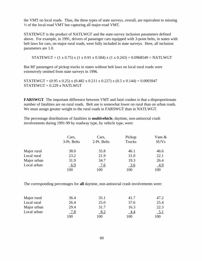
60

the VMT on local roads. Thus, the three types of state surveys, overall, are equivalent to missing½ of the local-road VMT but capturing all major-road VMT.

STATEWGT is the product of NATLWGT and the state-survey inclusion parameters definedabove. For example, in 1991, drivers of passenger cars equipped with 3-point belts, in states withbelt laws for cars, on major rural roads, were fully included in state surveys. Here, all inclusionparameters are 1.0.

STATEWGT = (1 x 0.75) x (1 x 0.91 x 0.584) x (1 x 0.243) = 0.0968549 = NATLWGT

But RF passengers of pickup trucks in states without belt laws on local rural roads wereextensively omitted from state surveys in 1996.

STATEWGT = (0.95 x 0.25) x (0.482 x 0.211 x 0.227) x (0.5 x 0.144) = 0.0003947STATEWGT = 0.229 x NATLWGT

FARSWGT The important difference between VMT and fatal crashes is that a disproportionatenumber of fatalities are on rural roads. Belt use is somewhat lower on rural than on urban roads. We must assign greater weight to the rural roads in FARSWGT than in NATLWGT.

The percentage distributions of fatalities in multivehicle, daytime, non-antisocial crashinvolvements during 1991-99 by roadway type, by vehicle type, were:

Cars, Cars, Pickup Vans &3-Pt. Belts 2-Pt. Belts Trucks SUVs

Major rural 38.0 35.8 46.1 46.6Local rural 23.2 21.9 31.0 22.1Major urban 31.9 34.7 19.3 26.4Local urban 6.9 7.6 3.6 4.9

100 100 100 100

The corresponding percentages for all daytime, non-antisocial crash involvements were:

Major rural 36.4 35.1 41.7 47.2Local rural 26.4 25.0 37.6 25.4Major urban 29.4 31.7 16.3 22.3Local urban 7.8 8.2 4.4 5.1

100 100 100 100

63For example, drivers constitute 75 percent of fatalities as well as occupants. While it istrue that passenger cars are overrepresented and light trucks are underrepresented amongoccupant fatalities, since we intend to compute UPFC separately for cars and light trucks, andnever to average the two, it is not necessary to develop new weights by vehicle type.

61

For the other parameters - seat position, belt law and vehicle type - we may use the same factors asNATLWGT63.

For example, in the multivehicle crashes, the FARSWGT for drivers of passenger cars equippedwith 3-point belts, in states with belt laws for cars, on major rural roads in 1991 is:

0.75 x 0.91 x 0.584 x 0.380 = 0.15146

and it is higher than NATLWGT (0.0968549), because fatality rates per VMT are higher on ruralroads.

Calibration of the belt-use-by-CY parameter We may now proceed to fill in the remaining gapin the model. Based on the STATEWGT factors for the 576 cells, and the linear effects of vehicletype, belt law, road type, and seat position on belt use that we have already calibrated, the leftcolumn of Table 18 shows exactly what percent driver belt use, on major urban roads, in belt-lawstates, in cars with 3-point belts, is needed in each calendar year to obtain exactly the overallaverage belt use reported in the state surveys. Those averages are shown in the right column ofTable 18, and they are copied from Table 14.

TABLE 18: CALIBRATION OF THE BELT-USE-BY-CY PARAMETER

Must have this belt use To obtain thisby drivers, cars, 3-pt. belts actual National averagemajor urban roads, belt law from state surveys

1991 62.8 58.31992 64.9 60.91993 69.1 65.01994 69.8 66.31995 71.4 67.11996 71.3 66.51997 72.5 67.51998 73.2 68.61999 74.9 70.1

The nine numbers in the left column drive the model, since the belt use rate in every cell can becomputed from one of them (or is already known, for cars with 2-point belts), and then averaged

62

using STATEWGT for a National average of the state surveys. For example, BELTUSE in 1991for drivers of passenger cars equipped with 3-point belts, in states with belt laws for cars, on majorrural roads is

62.8 - 3.6 = 59.2 percent

(where 62.8 percent is the 1991 belt use of drivers of cars with 3-point belts on major urban roadsin states with belt laws, as shown in Table 18, and 3.6 is the percentage point decrement for majorrural roads relative to major urban roads). The STATEWGT for this cell was derived earlier andfound to be 0.0968549.

For RF passengers of pickup trucks in states without belt laws on local rural roads in 1996,BELTUSE is

71.3 - 4.0 - 24.3 - 10.8 - 10.9 = 21.3 percent

(where 71.3 percent is the 1996 belt use of drivers of cars with 3-point belts on major urban roadsin states with belt laws, as shown in Table 18, and 4.0 is the percentage point decrement for the RFpassenger relative to the driver, 24.3 is the decrement for “no law,” 10.8 is the decrement forpickup trucks, and 10.9 is the decrement for local rural roads). The STATEWGT for this cell is0.0003947.

These examples illustrate the procedure for estimating BELTUSE in cars, pickup trucks andvans/SUVs with 3-point belts. The simpler procedure for cars with automatic 2-point belts wasdescribed earlier. When these BELTUSE numbers are averaged, weighted by STATEWGT, theywill yield exactly the VMT-weighted national averages of the state surveys, in each year, as shownin the right column of Table 18, or in Table 14.

Estimation of National on-the-road belt use The national average of the state surveys is anoverestimate of actual belt use on the road, especially before 1998, because a number of statesurveys did not include light trucks, RF passengers and/or local roads - where belt use is lowerthan for car drivers on major roads. But if the belt use rates in the 576 cells are weighted byNATLWGT rather than STATEWGT, they will yield national estimates of belt use on the road, foreach year from 1991 through 1999. Those estimates, at least in theory, ought to be directlycomparable to NOPUS, and subject to far less sampling error than NOPUS. Table 19 shows thesenational estimates for all vehicles, for passenger cars, and for light trucks. It also displays, forcomparison purposes, the unadjusted average of the state surveys (copied from Table 14), and theNOPUS results for 1994, 1996 and 1998.

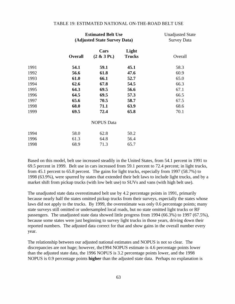
63

TABLE 19: ESTIMATED NATIONAL ON-THE-ROAD BELT USE

Estimated Belt Use Unadjusted State(Adjusted State Survey Data) Survey Data

Cars LightOverall (2 & 3 Pt.) Trucks Overall

1991 54.1 59.1 45.1 58.31992 56.6 61.8 47.6 60.91993 61.0 66.1 52.7 65.01994 62.6 67.8 54.5 66.31995 64.3 69.5 56.6 67.11996 64.5 69.5 57.3 66.51997 65.6 70.5 58.7 67.51998 68.0 71.1 63.9 68.61999 69.5 72.4 65.8 70.1

NOPUS Data

1994 58.0 62.8 50.21996 61.3 64.8 56.41998 68.9 71.3 65.7

Based on this model, belt use increased steadily in the United States, from 54.1 percent in 1991 to69.5 percent in 1999. Belt use in cars increased from 59.1 percent to 72.4 percent; in light trucks,from 45.1 percent to 65.8 percent. The gains for light trucks, especially from 1997 (58.7%) to1998 (63.9%), were spurred by states that extended their belt laws to include light trucks, and by amarket shift from pickup trucks (with low belt use) to SUVs and vans (with high belt use).

The unadjusted state data overestimated belt use by 4.2 percentage points in 1991, primarilybecause nearly half the states omitted pickup trucks from their surveys, especially the states whoselaws did not apply to the trucks. By 1999, the overestimate was only 0.6 percentage points; manystate surveys still omitted or undersampled local roads, but no state omitted light trucks or RFpassengers. The unadjusted state data showed little progress from 1994 (66.3%) to 1997 (67.5%),because some states were just beginning to survey light trucks in those years, driving down theirreported numbers. The adjusted data correct for that and show gains in the overall number everyyear.

The relationship between our adjusted national estimates and NOPUS is not so clear. Thediscrepancies are not huge; however, the1994 NOPUS estimate is 4.6 percentage points lowerthan the adjusted state data, the 1996 NOPUS is 3.2 percentage points lower, and the 1998NOPUS is 0.9 percentage points higher than the adjusted state data. Perhaps no explanation is

64Observed Safety Belt Use in 1996, NHTSA Research Note, Washington, 1997.

64

required: since the 2-sigma sampling error of NOPUS is ± 4 percentage points64, the discrepanciescan be considered within the “noise” range of NOPUS. They are substantially less than the 8.3percentage point discrepancy between 1994 NOPUS and the unadjusted state estimate, clearlybeyond sampling error bounds, and clearly due to the state surveys that omitted light trucks.

Less welcome explanations of why the adjusted state data exceed the early NOPUS could be thatour model does not fully correct for the state survey omissions in the earlier years, or even that thenon-probability sample designs of some early state surveys created upward biases that our modeldoes not address. However, if either of these are true - if the early adjusted state numbersoverestimate actual belt use - we can expect the effectiveness analysis later in this report tooverestimate fatality reduction in the earlier 1990's. As we shall see, it does not.

Belt effectiveness in daytime, non-antisocial crash involvements The final step of thevalidation analysis is to use the FARSWGT to estimate an on-the-road belt use we believe equal touse in potentially fatal crashes (U2 = U3), and in combination with the belt use of fatally injuredoccupants (U1), compute the fatality reduction by belts:

E = [U3 - U1] / [U3 - (U3 x U1)]

and compare it to the reductions obtained by double-pair comparison, adjusted by the UEF (Table13).

Table 20 computes belt use for our two populations of interest - front-outboard occupants ofpassenger cars equipped with 3-point belts, and of light trucks - on-the-road (using NATLWGT),and in potentially fatal crashes (using FARSWGT): multivehicle, and single + multivehicle daytime,non-antisocial crash involvements. Unlike Table 19, which combined 3-point and automatic 2-point belts into a single “passenger car” estimate for comparison with NOPUS, Table 20 is limitedto cars with 3-point belts.

Belt use on the road increased from 56.8 to 71.0 percent in cars with 3-point belts. These numbersare lower than in Table 19, because cars with automatic 2-point belts are excluded - but by 1999, itis only 1.4 percentage points lower (71.0 vs. 72.4), as the 2-point belts gradually phase out. Inlight trucks, it increased from 45.1 to 65.8 percent, as in Table 19. However, in potentially fatalmultivehicle crashes, belt use is 1.3 percentage points lower than on-the-road in cars, and 1.9percentage points lower than on-the-road in light trucks, because many of these crashes occur onrural roads, where belt use is lower. In single plus multivehicle crashes, belt use is yet another 0.3-0.5 percentage points lower, since an even greater proportion of the single-vehicle crashes arerural.

65

TABLE 20: BELT USE ON-THE-ROAD AND IN POTENTIALLY FATAL CRASHES

In Potentially Fatal, DaytimeOn Non-Antisocial Crash Involvementsthe

Road Multivehicle Single + Multi

Cars Light Cars Light Cars Light(3 Pt.) Trucks (3 Pt.) Trucks (3 Pt.) Trucks

1991 56.8 45.1 55.5 43.2 55.2 42.71992 59.4 47.6 58.1 45.7 57.8 45.21993 63.7 52.7 62.5 50.8 62.2 50.31994 65.4 54.5 64.2 52.6 63.8 52.11995 67.3 56.6 66.1 54.7 65.8 54.21996 67.4 57.3 66.1 55.4 65.8 54.91997 68.6 58.7 67.3 56.8 67.0 56.31998 69.3 63.9 68.0 62.0 67.7 61.51999 71.0 65.8 69.7 63.9 69.4 63.4

TABLE 21: FATALITY REDUCTION BASED ON UPFC, CARS WITH 3-POINT BELTSMULTIVEHICLE DAYTIME, NON-ANTISOCIAL CRASH INVOLVEMENTS

Belt Use (%)Fatality

Fatalities UPFCs Reduction (%)(U1) (U2 = U3) (E)

1991 49.0 55.5 23.11992 50.2 58.1 27.41993 54.6 62.5 27.81994 57.2 64.2 25.31995 57.2 66.1 31.41996 59.6 66.1 24.41997 61.3 67.3 23.11998 63.6 68.0 17.91999 63.7 69.7 23.8

Average 24.9Standard Deviation / /9 1.3

65If the adjusted state data had overestimated actual belt use in the earlier years, we wouldhave expected higher effectiveness in those years, and low effectiveness later on.

66Table 22 shows higher fatality reduction in 1998-99 than in preceding years, due to a1998 jump in our estimated U2 that exceeds the steady year-to-year gains in U1. Two factors maybe at work. (1) The accelerating market shift from pickup trucks to SUVs could increaseeffectiveness over time, since belts appear to be more effective in SUVs than in pickup trucks (seeTable 12 and its discussion). (2) Traffic Safety Facts (op. cit.) suggests all state belt lawsencompassed light trucks in 1998, but quite a few did not in 1997. Our method may haveunderstated belt use in light trucks in the last years before 1998 in the “no law” states, or theremay have been additional states that extended their belt laws to light trucks before 1998. Notwithstanding the jump in 1998, we believe the 1991-99 average effectiveness is accurate.

66

Table 21 performs the effectiveness analysis for passenger cars with 3-point belts in multivehicle,daytime non-antisocial crash involvements. It is remarkable how the belt use in potentially fatalcrashes, based on adjusted state survey data, rises in tandem with the belt use rate of fatally injuredoccupants, based on FARS. Belt effectiveness, E = [U3 - U1] / [U3 - (U3 x U1)], is close to 25percent in this special group of crashes, year after year65. The average of the nine annual estimatesis 24.9 percent. The standard deviation of the nine individual estimates, divided by /9, is thestandard error of the nine-year average. The 1.96ó sampling-error range for effectiveness is24.9 ± 2.5 percent. (This interval estimate is not presented as “confidence bounds” but as anindicator of minimum sampling error that could be augmented by non-sampling errors introducedby the various assumptions in the model.)

In multivehicle, daytime, non-antisocial crash involvements, the effectiveness estimate based ondouble-pair comparison analysis of 1986-99 FARS data, corrected by the UEF, is 29 ± 10 percent,as shown in Table 13. Thus, our interval estimate based on belt use among fatalities (1991-99FARS) and UPFC (1991-99 state surveys), 24.9 ± 2.5 percent, is well within the minimumsampling error range of the double-pair comparison analysis, 29 ± 10 percent. It validates the useof double-pair comparison, when corrected by the UEF, on post-1986 FARS data.

The remaining three analyses agree even more closely with the double-pair comparison results ofTable 13. Table 22 analyzes light trucks in multivehicle, daytime non-antisocial crashinvolvements.

Again, UPFC keeps a steady lead over U1, but by a greater margin than in Table 21, resulting in ahigher effectiveness. The sampling error range for this estimate, 39.3 ± 3.7 percent is entirelywithin the interval estimate based on double-pair comparison, 42 ± 12 percent, and the pointestimates are quite close66.

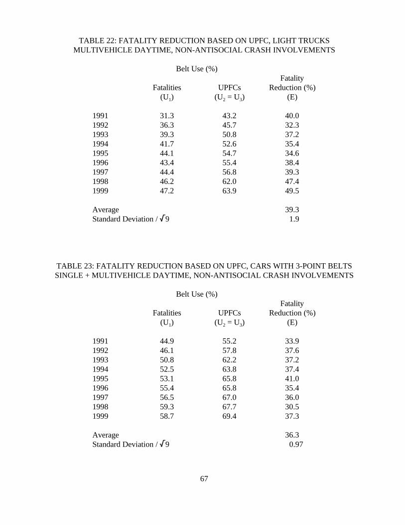
67

TABLE 22: FATALITY REDUCTION BASED ON UPFC, LIGHT TRUCKSMULTIVEHICLE DAYTIME, NON-ANTISOCIAL CRASH INVOLVEMENTS



1991 31.3 43.2 40.01992 36.3 45.7 32.31993 39.3 50.8 37.21994 41.7 52.6 35.41995 44.1 54.7 34.61996 43.4 55.4 38.41997 44.4 56.8 39.31998 46.2 62.0 47.41999 47.2 63.9 49.5


TABLE 23: FATALITY REDUCTION BASED ON UPFC, CARS WITH 3-POINT BELTSSINGLE + MULTIVEHICLE DAYTIME, NON-ANTISOCIAL CRASH INVOLVEMENTS



1991 44.9 55.2 33.91992 46.1 57.8 37.61993 50.8 62.2 37.21994 52.5 63.8 37.41995 53.1 65.8 41.01996 55.4 65.8 35.41997 56.5 67.0 36.01998 59.3 67.7 30.51999 58.7 69.4 37.3


67Table 24, like Table 22, shows higher effectiveness in 1998-99. See the discussion inFootnote 61.

68

Table 23 returns to passenger cars with 3-point belts, but expands the analysis to all daytime, non-antisocial crash involvements - single plus multivehicle. This analysis is based on the largest N ofFARS cases, and shows the highest year-to-year consistency for fatality reduction. Theeffectiveness estimate, 36.3 ± 1.9 percent is well within the interval estimate based on double-paircomparison, 38 ± 8 percent, and the two point estimates are quite close.

Table 24 analyzes light trucks in single plus multivehicle crashes.

TABLE 24: FATALITY REDUCTION BASED ON UPFC, LIGHT TRUCKSSINGLE + MULTIVEHICLE DAYTIME, NON-ANTISOCIAL CRASH INVOLVEMENTS



1991 27.4 42.7 49.31992 32.0 45.2 42.91993 33.4 50.3 50.41994 35.6 52.1 49.11995 37.8 54.2 48.61996 37.8 54.9 50.21997 39.4 56.3 49.61998 40.7 61.5 57.01999 39.4 63.4 62.5


The interval estimate of fatality reduction is 51.1 ± 3.7 percent and it is very compatible with the52 ± 8 percent generated by double-pair comparison. Indeed, all four analyses here validate theircounterpart estimates based on double-pair comparison67.

This method based on UPFC generates effectiveness estimates with less sampling error than thecorresponding double-pair comparisons. The reader will be tempted to ask, “Why did we limit theanalyses to just these special groups of fatal crashes? Why couldn’t we use this method directly toestimate the overall fatality reduction by safety belts?” The answer, of course, is that this methodonly works for subgroups of fatalities where it is plausible that the UPFC is equal to belt useobserved on the road. For the full set of fatalities, including alcohol-impaired drivers, reckless

68Specifically, the belt use rate of all passenger-vehicle front-outboard fatalities in 1991-99was 36.6 percent and the average 1991-99 belt use rate on the road, based on the adjusted statedata (Table 19, left column) was 62.9 percent. That works out to 66 percent effectiveness forbelts.

69Final Regulatory Impact Analysis (1984), p. IV-2.

69

drivers and nighttime crashes, UPFC is much lower than belt use observed in surveys, and thismethod would greatly overestimate effectiveness68.

However, we can compare the UPFC-based and double-pair comparison estimates for thesesubgroups of fatalities and, based on ratios, assess the implications for the full set of fatalities. Forcars with 3-point belts in multivehicle, daytime, non-antisocial crash involvements, the fatalityreduction is 24.9 percent based on the UPFC analysis (Table 21) and 29 percent based on double-pair comparison (Table 13). Since the overall effectiveness of belts is 45 percent, based on double-pair comparison (Table 1), the implicit effectiveness for all crashes, by the UPFC method would be

1 - {[(1 - 0.249) / (1 - 0.29)] x [1 - 0.45]} = 41.8 percent

For cars with 3-point belts in single + multivehicle, daytime, non-antisocial crash involvements, thefatality reduction is 36.3 percent with UPFC (Table 23) and 38 percent with double-paircomparison (Table 13). The implicit effectiveness for all crashes, by the UPFC method would be

1 - {[(1 - 0.363) / (1 - 0.38)] x [1 - 0.45]} = 43.5 percent

Both of these numbers are well within the 40 to 50 percent range that NHTSA estimated for safetybelt effectiveness in 1984 and still uses as its “official” estimate69. They are also well within the“noise” range of the UEF-corrected double-pair comparison estimate of 45 percent fatalityreduction by 3-point belts in passenger cars.

For light trucks in multivehicle, daytime, non-antisocial crash involvements, the fatality reduction is39.3 percent with UPFC (Table 22) and 42 percent with double-pair comparison (Table 13). Since the overall effectiveness of belts is 60 percent, based on double-pair comparison (Table 1),the implicit effectiveness for all crashes, by the UPFC method would be

1 - {[(1 - 0.393) / (1 - 0.42)] x [1 - 0.60]} = 58.1 percent

In the single + multivehicle crashes, the fatality reduction is 51.1 percent with UPFC (Table 24)and 52 percent with double-pair comparison (Table 13). The implicit effectiveness for all crashes,with UPFC would be

1 - {[(1 - 0.511) / (1 - 0.52)] x [1 - 0.60]} = 59.3 percent

70Preliminary Regulatory Impact Analysis (1989), p. 15.

70

Both of these numbers are close to NHTSA’s “official” 60 percent estimate70 and well within the“noise” range of the UEF-corrected double-pair comparison estimate of 60 percent fatalityreduction by belts in light trucks.

Conclusion The relatively high rate of belt use among fatally injured occupants in daytime, non-drinking, non-antisocial crash involvements shows it is very unlikely that belt effectiveness couldbe 60+ percent in cars, or 70+ percent in light trucks, as suggested by uncorrected double-paircomparison. These analyses of belt use on the road versus belt use of fatally injured occupantssupport NHTSA’s long-standing estimates that safety belts reduce fatalities by close to 45 percentin cars and 60 percent in light trucks. They support the use of the UEF, as defined in Section 5, toadjust downwards the estimates based on double-pair comparison of FARS data collected after1985.

71

REFERENCES

Blincoe, Lawrence J. Estimating the Benefits from Increased Safety Belt Use. NHTSAPublication No. DOT HS 808 133, Washington, 1994.

Bowman, Brian L. and Rounds, Donald A. Restraint System Usage in the Traffic Population -1988 Annual Report. NHTSA Publication No. DOT HS 807 447, Washington, 1989.

Cerrelli, Ezio. Driver Exposure: Indirect Approach for Obtaining Relative Measures. NHTSAPublication No. DOT HS 820 179, Washington, 1972.

Evaluation of the Effectiveness of Occupant Protection - Federal Motor Vehicle Safety Standard208 - Interim Report, June 1992. NHTSA Publication No. DOT HS 807 843, Washington, 1992.

Evans, Leonard. “Double Pair Comparison - A New Method to Determine How OccupantCharacteristics Affect Fatality Risk in Traffic Crashes.” Accident Analysis and Prevention, Vol.18, June 1986, pp. 217-227.

_________. “The Effectiveness of Safety Belts in Preventing Fatalities.” Accident Analysis andPrevention, Vol. 18, June 1986, pp. 229-241.

_________. Traffic Safety and the Driver. Van Nostrand Reinhold, New York, 1991.

Evans, Leonard and Frick, Michael C. “Potential Fatality Reductions through EliminatingOccupant Ejection from Cars.” Accident Analysis and Prevention, Vol. 21, pp. 169-182.

Final Regulatory Impact Analysis, Amendment to Federal Motor Vehicle Safety Standard 208,Passenger Car Front Seat Occupant Protection. NHTSA Publication No. DOT HS 806 572,Washington, 1984.

Fourth Report to Congress, Effectiveness of Occupant Protection Systems and their Use. NHTSA Publication No. DOT HS 808 919, Washington, 1999.

Haight, Frank A. Indirect Methods for Measruing Exposure Factors as Related to the Incidenceof Motor Vehicle Traffic Accidents. NHTSA Publication No. DOT HS 800 601, Washington,1971.

Hansen, Morris H., Hurwitz, William N., and Madow, William G. Sample Survey Methods andTheory, Volume I. John Wiley & Sons, New York, 1953.

Kahane, Charles J. Addendum to "Seat Belt Effectiveness Estimates Using Data Adjusted forDamage Type”. NHTSA Docket No. 74-14-N35-229-05, 1984.

72

_________. An Evaluation of Door Locks and Roof Crush Resistance of Passenger Cars. NHTSA Publication No. DOT HS 807 489, Washington, 1989.

_________. Evaluation of FMVSS 214 - Side Impact Protection: Dynamic Performance. NHTSA Publication No. DOT HS 809 004, Washington, 1999.

Klein, Terry M. A Method for Estimating Posterior BAC Distributions for Persons Involved inFatal Traffic Accidents. NHTSA Publication No. DOT HS 807 094, Washington, 1986.

Klein, Terry M. and Walz, Marie C. Estimating Lives Saved by Restraint Use in Potentially FatalCrashes. NHTSA Research Note, Washington, 1995.

Mosteller, F. and Tukey, J.W. Data Analysis and Regression: A Second Course in Statistics. Addison-Wesley, Reading, MA, 1977.

National Occupant Protection Use Survey. Washington Consulting Group, Washington, 1995.

Observed Safety Belt Use in 1996. NHTSA Research Note, Washington, 1997.

Partyka, Susan C. “Belt Effectiveness in Pickup Trucks and Passenger Cars by Crash Directionand Accident Year (May 1988).” Papers on Adult Seat Belts - Effectiveness and Use. NHTSAPublication No. DOT HS 807 285, Washington, 1988.

_________. Belt Use in Serious Impacts Estimated from Fatality Data. NHTSA Publication No.DOT HS 807 519, Washington, 1989.

_________. Lives Saved by Seat Belts from 1983 through 1987. NHTSA Publication No. DOTHS 807 324, Washington, 1988.

_________. “Seat Belt Effectiveness Estimates Using Data Adjusted for Damage Type (January1984).” Papers on Adult Seat Belts - Effectiveness and Use. NHTSA Publication No. DOT HS807 285, Washington, 1988.

Partyka, Susan C. and Womble, Kathleen B. Projected Lives Savings from Greater Belt Use. NHTSA Research Note, Washington, 1989.

Preliminary Regulatory Impact Analysis, Proposed Extension of the Automatic RestraintRequirements of FMVSS 208 to Trucks, Buses and Multi-Purpose Passenger Vehicles with aGross Vehicle Weight Rating of 8,500 Pounds or Less and an Unloaded Vehicle Weight of 5,000Pounds or Less. NHTSA Docket No. 74-14-N62-001, 1989.

Reinfurt, Donald W., Silva, Claudio Z. and Seila, Andrew F. A Statistical Analysis of Seat BeltEffectiveness in 1973-75 Model Cars Involved in Towaway Crashes, Volume 1. NHTSAPublication No. DOT HS 802 035, Washington, 1976.

73

Rood, Debra H., Kraichy, Patricia P. and Carubia, Jean. Evaluation of New York State’sMandatory Occupant Restraint Law. NHTSA Publication No. DOT HS 806 950, Washington,1985.

Safety Belt Usage, A Review of Effectiveness Studies, Suggestions for State Programs. NHTSAPublication No. DOT HS 801 988, Washington, 1976.

Sikora, James J. Relative Risk of Death for Ejected Occupants in Fatal Traffic Accidents. NHTSA Publication No. DOT HS 807 096, Washington, 1986.

Teets, Mary K. Highway Statistics 1993. Publication No. FHWA-PL-94-023, Federal HighwayAdministration, Washington, 1994.

Traffic Safety Facts 1998. NHTSA Publication No. DOT HS 808 983, Washington, 1999.

Wagnenaar, A.C., Wiviott, M.B.T. and Compton, C.P. Direct Observation of Seat Belt Use inMichigan: April 1985. Publication No. UMTRI 85-26, University of Michigan TransportationResearch Institute, Ann Arbor, 1985.

APPENDIX: STATE BELT USE SURVEYS AND LAWS, 1991-99

OBSERVED BELT USE (%) Belt Law Effective VMT 91-97 1998 9 9 9 9 9 9 9 9 9 Van/ Survey (Million) 1 2 3 4 5 6 7 8 9 Car P/U SUV Omits Survey Type

Alabama 54,870 53 58 55 55 52 54.0 52.0 52.0 58.1 91½ 98 98 ADT RoadsAlaska 4,489 66 66 69 69 69 53.0 56.0 57.0 64.0 * * * UnknownArizona 45,209 65 73 73 60 60 55.9 63.2 61.5 71.9 91 98 91 Signalized X-sectionArkansas 28,170 52 55 55 51 51 48.0 50.5 52.6 57.2 91½ 91½ 91½ ADT RoadsCalifornia 284,642 71 70 83 83 85 86.6 86.4 88.6 89.3 * * * Other Local-roadColorado 39,039 51 50 53 54 56 55.6 59.6 66.0 65.2 * * * Non-WESTAT Unk TypeConnecticut 29,142 61 71 71 72 72 59.4 59.8 70.1 72.5 * * * WESTAT SurveyDelaware 8,165 42 70 68 63 60 62.0 59.0 62.3 64.4 92 98 98 Non-WESTAT Unk TypeD.C. 3,282 49 59 62 62 63 57.0 66.0 79.6 77.9 * * * LT+RF WESTAT SurveyFlorida 136,624 60 57 62 61 59 62.7 60.0 57.2 59.0 * * * UnknownGeorgia 96,430 54 51 57 57 53 58.0 65.0 73.6 74.2 * 96 * ADT RoadsHawaii 7,929 85 83 84 84 85 78.3 80.0 80.5 80.3 * * * WESTAT SurveyIdaho 13,337 45 53 59 61 59 50.0 49.0 57.3 57.3 * * * Non-WESTAT Unk TypeIllinois 100,630 51 65 67 68 69 64.0 64.2 64.5 65.9 * * * LT ADT RoadsIndiana 68,443 52 56 56 56 64 52.7 53.2 61.8 57.3 * 98 98 Non-WESTAT Unk TypeIowa 28,722 68 71 73 73 76 74.8 74.9 76.9 78.2 * * * Other Local-roadKansas 26,936 64 70 70 70 54 54.0 56.0 58.7 62.6 * 98 * Other Local-roadKentucky 46,285 48 41 40 58 52 55.0 54.0 54.3 58.6 94½ 94½ 94½ RF UnknownLouisiana 40,063 37 47 48 50 59 59.0 64.0 65.6 67.0 * * * WESTAT SurveyMaine 13,468 35 36 36 36 50 50.0 61.0 61.3 59.0 96 96 96 Signalized X-sectionMaryland 48,044 72 75 72 69 70 70.0 71.0 82.6 82.7 * * * ADT RoadsMassachusetts 51,510 35 31 34 47 53 54.0 53.0 51.0 52.0 94 94 94 Signalized X-sectionMichigan 93,332 64 53 64 66 67 66.1 66.9 69.9 70.1 * * * Signalized X-sectionMinnesota 49,331 52 53 55 57 65 64.0 64.8 64.2 71.5 * * * WESTAT SurveyMississippi 33,999 32 24 25 43 46 46.0 48.2 58.0 54.5 * 98 * LT WESTAT SurveyMissouri 64,138 54 70 70 68 71 62.0 66.6 60.4 60.8 * 98 * LT+RF Non-WESTAT Unk TypeMontana 9,530 67 71 71 69 70 70.8 72.6 73.1 74.0 * * * Other Local-road

*In effect before 1991

OBSERVED BELT USE (%) Belt Law Effective VMT 91-97 1998 9 9 9 9 9 9 9 9 9 Van/ Survey (Million) 1 2 3 4 5 6 7 8 9 Car P/U SUV Omits Survey Type

Nebraska 17,459 33 33 54 63 64 64.6 62.9 65.1 67.9 93 93 93 Other Local-roadNevada 17,196 68 63 70 71 71 70.1 69.4 76.2 79.8 * 98 98 ADT RoadsNew Hampshire 11,499 49 50 51 54 57 56.0 57.7 55.6 56.0 N E V E R UnknownNew Jersey 64,111 58 68 71 64 61 60.3 62.0 63.0 63.3 * 98 98 LT WESTAT SurveyNew Mexico 22,053 67 66 75 79 86 85.0 88.0 82.6 88.4 * * * Non-WESTAT Unk TypeNew York 122,605 68 69 72 72 72 73.6 75.2 75.3 76.1 * 98 98 LT WESTAT SurveyNorth Carolina 84,747 60 70 80 81 81 80.0 82.0 76.7 78.1 * 93 * Signalized X-sectionNorth Dakota 7,299 30 30 30 32 42 41.8 49.4 40.0 46.7 94½ 94½ 94½ Non-WESTAT Unk TypeOhio 104,280 50 58 62 62 62 62.4 65.2 60.6 64.8 * * * LT Non-WESTAT Unk TypeOklahoma 41,770 37 44 47 45 46 47.5 60.0 56.0 60.7 * * * UnknownOregon 33,158 70 72 73 77 80 81.5 82.1 82.6 83.4 * 94 94 Signalized X-sectionPennsylvania 99,291 60 63 68 72 71 65.0 65.0 67.8 69.7 * * * Other Local-roadRhode Island 7,929 28 32 32 58 58 59.0 59.0 58.6 67.3 91½ 98 98 ADT RoadsSouth Carolina 42,557 60 53 59 64 64 61.1 60.8 64.8 65.0 * * * UnknownSouth Dakota 8,034 33 42 26 40 40 47.0 68.0 45.7 45.7 95 95 95 Non-WESTAT Unk TypeTennessee 62,169 51 58 58 60 64 63.0 61.0 56.7 61.3 * * * LT WESTAT SurveyTexas 204,726 68 69 69 71 72 74.0 74.6 74.4 74.0 * * * Signalized X-sectionUtah 21,134 45 50 50 53 56 60.1 62.9 66.7 67.4 * * * Non-WESTAT Unk TypeVermont 6,563 40 47 54 68 67 68.5 70.9 62.7 69.8 94 98 98 Non-WESTAT Unk TypeVirginia 70,255 58 72 73 72 70 69.6 67.1 73.6 69.9 * * * Signalized X-sectionWashington 51,615 69 73 78 81 83 83.2 81.4 79.1 81.1 * * * LT WESTAT SurveyWest Virginia 18,561 43 34 52 58 58 64.0 67.0 56.5 51.9 94 98 98 RF Signalized X-sectionWisconsin 55,448 58 59 64 64 64 58.1 51.6 61.9 65.1 * * * Signalized X-sectionWyoming 7,981 66 66 67 70 71 58.5 59.5 50.1 50.1 * * * Unknown

*In effect before 1991

Fatality Reduction by Safety Belts

Documents

Transcript of Fatality Reduction by Safety Belts