Fastparallelevaluationofexactgeometricpredicateson GPUs

Fast parallel evaluation of exact geometric predicates onGPUs

Marcelo de Matos Menezesa, Salles Viana Gomes de Magalhãesb, MatheusAguilar de Oliveirac, W. Randolph Franklind, Rodrigo Eduardo de Oliveira

Bauer Chichorroe

aUniversidade Federal de Viçosa (MG) Brasil, [email protected] Federal de Viçosa (MG) Brasil, [email protected]

cUniversidade Federal de Viçosa (MG) Brasil, [email protected] Polytechnic Institute, Troy NY, USA 12180, [email protected]

eUniversidade Federal de Viçosa (MG) Brasil, [email protected]

AbstractThis paper accelerates the exact evaluation of large numbers of 3D geometricpredicates with an algorithm whose work is partitioned between the CPU andthe GPU on a high-performance computer to exploit the relative strengthsof each. The test algorithm computes all the red–blue intersections betweena set of red 3D triangles and another set of blue 3D triangles. A sequenceof filters is employed that progressively eliminates more and more red–bluepairs that do not intersect, finally leaving only the actual intersections. Ini-tially, a uniform grid is constructed on the GPU to identify pairs of nearbytriangles. Then, these pairs are tested for intersection with single-precisioninterval arithmetic on the GPU. The ambiguous cases are next filtered withdouble-precision interval arithmetic on the multi-core CPU, and finally thehard cases are re-evaluated in parallel on the CPU using arbitrary-precisionrational numbers. The parallel speedup for the whole algorithm was up to414 times. It took only 1.17 seconds to find the 18M intersections betweentwo datasets containing a total of 14M triangles. The intersection computa-tion was sped up by up to 1936 times. The techniques that gave this excellentperformance should be useful for parallelizing other geometric algorithms infields such as CAD, GIS, and 3D modeling.

Keywords: Geometric predicates; Parallel programming; Exactcomputation; Polyhedron intersection

Preprint submitted to Computer-Aided Design November 29, 2021

1. Introduction

Addressing the errors caused by floating-point arithmetic is a particularchallenge in computational geometry. Inexact floating-point numbers violatemost of the axioms of an algebraic field, e.g., addition is not associative.Roundoff errors lead to topological errors such as causing an orientationpredicate to report a point to be on the wrong side of a line segment. Theseerrors may then propagate to higher-level operations, such as arise whenusing orientation predicates to compute a convex hull.

While there are heuristics, such as epsilon-tweaking and snap rounding,that try to solve this, they are not guaranteed to always work.

Representing coordinates with exact arbitrary-precision rational numbersguarantees that the computation will be free from round-off errors. However,the run-time overhead is often unacceptable. Indeed, the total number ofdigits in the numerator and denominator of the output is typically the sumof the numbers of digits in the operands, and so grows exponentially withthe depth of the computation tree. Likewise, the time and space cost of eachoperation will grow exponentially with the computation tree’s depth, badlydegrading performance.

Some techniques have been proposed to cope. Arithmetic filters usinginterval arithmetic represent each exact number e as an interval [l, h] offloating-point values containing e. The IEEE-754 floating-point standardguarantees that, for each arithmetic operation, a new interval guaranteedto contain the exact result can be computed. Thus, a predicate can be ini-tially evaluated using intervals. If the exact result can be inferred from thebounds of the interval, then this result is returned. Otherwise, the expres-sion is re-evaluated, either with exact arithmetic, or with intervals that havemore precise number types. Most of the time, computation with intervals isenough to infer the exact result [? ], and so predicates can be efficiently andexactly evaluated without the overhead of exact computation.

The computing capabilities of desktop computers and workstations haverecently increased due to multi-core processors and accelerators such as GPG-PUs (General Purpose Graphics Processing Units) and MICs (Many Inte-grated Core Architectures). However, many algorithms cannot take advan-tage of this because they are still designed for sequential architectures

This paper proposes to combine GPUs and multi-core CPUs, using theparticular strengths of each, to accelerate the evaluation of exact predicatesusing arithmetic filters. Our idea is to use the parallel processing power of

the GPU to quickly evaluate a batch of predicates using interval arithmetic.GPUs are designed for fast floating point calculations, which makes themsuitable for interval arithmetic. The few unreliable results are detected andre-evaluated in parallel on the CPU using exact arithmetic.

A preliminary version of this framework has been implemented and testedfor computing the intersections between two sets of 2D segments [? ]. Thisemploys a uniform grid to cull the number of segments. The CPU traversesthe grid and creates a list of pairs of segments, which is sent to the GPU for in-tersection evaluation using interval arithmetic. The results are then returnedto the CPU. They are represented with a flag with 3 possible values: inter-section, no intersection, or uncertain result (interval failure). Interval failuremeans this intersection cannot be safely determined using intervals. TheCPU processes each interval failure by recomputing the intersection usingmultiple-precision rational numbers. Compared to a sequential implemen-tation, the algorithm achieved speedups of up to 289 times for intersectionevaluation, and up to 40 times when the entire running time is included, onan NVIDIA GTX 1070 Ti GPU.

In [? ], we extended this to compute intersections between segmentsand triangles in 3D. The initial version performed badly because the pre-processing step, where the CPU creates a list of pairs of segments and trian-gles, was a bottleneck. Thus in [? ] we proposed a new method using threeauxiliary arrays to associate each GPU thread with the (segment, triangle)pairs assigned to it for testing.

This implementation led to a speedup of up to 17 times on a NVIDIAGTX 1070 Ti GPU, compared to a sequential implementation. Besides thefact that 3D predicates are more complex than 2D, which leads to morethread divergence, another reason for the smaller speedup of the 3D version isthat a bounding-box culling step was added before the intersection tests. Thisimproved the performance, but the improvement in the sequential version wasbetter than in the parallel one. The problem was that the bounding-box testincreased the GPU thread divergence. The issue is that GPU threads aregrouped by 32s into warps, and all the threads in one warp must execute thesame instruction or be idle.

Finally, in this paper, we extend the framework in three ways. First, weimprove the bounding-box step to increase the parallel speedup. Second, wecreate the array of pairs on the GPU. Third, we use single-precision floating-point arithmetic, instead of double-precision, for the intervals, because onGPUs, single is usually several times faster. We correct for the reduced

precision of single-precision as follows. Unreliable single-precision results areidentified by using interval arithmetic. They are re-evaluated with double-precision, and if still unreliable, with rationals.

We evaluated these novel ideas with a new case study, described in Sec-tion 4. It detects the pairwise intersections of 3D triangles from two meshes.Experiments were performed on the newer and faster NVIDIA RTX 8000GPU. We observed a speedup of up to 1936 times for intersection evalua-tion compared to a sequential implementation. The speedup for the entirerunning time was up to 414 times. On the older GTX 1070 Ti GPU, the par-allel speedup for the intersection computation was 407×, and for the entirerunning time was 158×.

The performance and correctness make this technique an excellent choicefor processing large datasets, where the chance of failure from inexact algo-rithms is higher, in interactive applications such as GIS and CAD systems.

2. Background

2.1. Roundoff errorsNon-integers are typically approximately represented in computers with

floating-point values. The difference between a non-integer and its approx-imation is called the roundoff error. Although these differences are usuallysmall, these errors accumulate as sequences of arithmetic operations are per-formed. The presence of floating point errors in computer programs can haveserious consequences in diverse fields such as the failures of the first ArianeV rocket [5] and the Patriot missile defense system [19].

In geometry, roundoff errors can generate topological inconsistencies caus-ing globally impossible results. For example, the computed intersection oftwo line segments may not lie on either line. Kettner et al. [14] gave someexamples of failures that can cause algorithms, e.g. for computing convexhulls, to fail.

The planar orientation predicate says whether three 2D points p = (px, py),q = (qx, qy), r = (rx, ry) are collinear, make a left turn, or make a right turn.It is the sign of the following determinant:∣∣∣∣∣∣

px py 1qx qy 1rx ry 1

∣∣∣∣∣∣

Figure 1: Roundoff errors in the planar orientation problem - Geometry of the planarorientation predicate for double precision floating point arithmetic. Yellow, red and bluepoints represent, respectively, collinear, negative and positive orientations. The diagonalline is an approximation of the segment (q, r). What should happen is that all the pixelsabove the line are blue, and all those below are red. Source: [14].

Positive, negative and zero signs mean that (p, q, r), respectively, makea left turn, right turn or are collinear. Roundoff errors may cause the signof this determinant to be evaluated wrongly, mis-classifying the orientation.To illustrate this problem, Kettner et al. [14] implemented a program toapply the planar orientation predicate (orientation(p, q, r)) to a point p =(px+xu, py+yu), where u is the step between adjacent floating point numbersof size around p, and 0 ≤ x, y ≤ 255. This results in a 256 × 256 matrixcontaining either blue, yellow and red points, where the colors mean thatthe corresponding point is computed to be above, on or below the line thatpasses through q and r. Figure 1 shows this experiment for p = (0.5, 0.5),u = 2−53, q = (12, 12) and r = (24, 24). Several points have orientationscomputed incorrectly.

As shown by [14], these inconsistent results in the orientation predicatescould make algorithms that use this predicate to fail.

There are various proposed solutions. The simplest one, epsilon-tweaking,uses an ε tolerance, and considers two values x and y equal if |x − y| ≤ε. However this is a formal mess because equality is neither transitive norinvariant under scaling. Thus, in practice, epsilon-tweaking can fail [14].

Snap rounding is another method to approximately represent arbitraryprecision segments on a fixed-precision grid [9]. However, snap rounding cangenerate inconsistencies, and deform the original topology if applied repeat-edly on the same data set. Some possible solutions are presented in [4, 8, 2].

Shewchuk [18] presents the Adaptive Precision Floating-Point techniquefor exactly evaluating predicates. The evaluation is performed using the onlyminimum precision necessary to achieve correctness. That allows some effi-cient exact geometric algorithms to be developed. Many geometric predicatesreduce to computing the sign of a determinant. So, the precise value of thisdeterminant does not need to be computed as long as its sign is correct. Todetermine if the sign can be trusted, the approximation and an error esti-mate are computed. If the error is big enough to make the sign uncertain,the values are recomputed using higher precision. However, this techniqueis not suitable for solving all geometric problems [18]. For example, “a pro-gram that computes line intersections requires rational arithmetic; an exactnumerator and exact denominator must be stored” [18].

The proper formal way to eliminate roundoff errors and guarantee algo-rithm robustness is to use exact computation with arbitrary precision rationalnumbers [15, 11, 14? ]. Computing in the algebraic field of rational num-bers over the integers, with the integers allowed to grow as large as necessary,allows the traditional arithmetic operations, +,−,×,÷, to be computed ex-actly with no roundoff error.

The cost is that the number of digits resulting from an operation is aboutequal to the sum of the numbers of digits in the two inputs. E.g., 214

433+

659781

= 452481338173

. Casting out common factors helps only to a small degree.However, this growth is acceptable if the depth of the computation tree issmall. Also, the cost can be significantly reduced by employing techniquessuch as arithmetic filtering with interval arithmetic, as we will discuss inSection 2.2.

2.2. Arithmetic filters and interval arithmeticOne technique to accelerate algorithms based on exact arithmetic is to

employ arithmetic filters and interval arithmetic [16]. Each floating-pointnumber is represented by an interval containing the exact value. During apredicate evaluation, such as the computation of the sign of an arithmeticexpression, the arithmetic operations are initially applied to the intervals.The resulting interval is computed so as to guarantee that it will containthe exact result of the operation (this is called the containment property).Finally, if the bounds of the resulting interval have the same sign, so thatthe sign of the exact result is known, that value is returned. Otherwise, thepredicate is re-evaluated using exact arithmetic instead of the floating-point

intervals. The term arithmetic filter derives from the process of filtering theunreliable results and recomputing them with exact arithmetic.

This is possible and efficient because the IEEE-754 floating-point numberstandard defines how arithmetic operations are approximated: “the result ofoperations can be seen as if they were performed exactly, but then roundedto one of the nearest floating-point values enclosing the exact value” [16].IEEE-754 defines three rounding-modes, selectable at runtime: rounding tothe nearest representable floating-point value, or down towards −∞ (i.e.,the closest smaller representable floating-point number), or up towards +∞(the closest larger representable floating-point number). So, the intervalcontainment property can be maintained.

CGAL [16] illustrates this process with addition. Suppose xInterval =[x.lower, x.upper] and yInterval = [y.lower, y.upper] are, respectively, floating-point intervals containing the exact values xExact and yExact. The floating-point interval [x.lower ± y.lower, x.upper ∓ y.upper] (where ± and ∓ rep-resent, respectively, rounding towards −∞ or +∞) is guaranteed to containthe exact value of the expression xExact+ yExact.

The Computational Geometry Algorithms Library (CGAL) [3] supportsexact computation because its framework makes it easy to develop algorithmsthat combine one of its number types, arbitrary precision rational numbers,with arithmetic filters.

There are multiple types of arithmetic filters [16]. Listing 1 shows one.Here, variables with the suffix _exact were created as GMP[7] (GNU Mul-tiple Precision Arithmetic Library) arbitrary precision rationals (of typempq_class) while the ones with suffix _interval use CGAL’s interval arith-metic number type. Both types overload the arithmetic and boolean oper-ators. If the comparison (line 8) cannot be evaluated safely, CGAL throwsan unsafe_comparison exception. When it is caught, that predicate can bere-evaluated using the exact version of the respective variables (line 14).

Evaluating a sequence of operations is challenging because we may notknow the exact value of the operands (since they were generated by severaloperations). CGAL provides a more generic and reusable type of filter thatsolves this by using a directed acyclic graph (DAG) to represent the historyof the operations that generated each geometric object.

This is transparent to the user, and does not require an explicit try...catch block as used in Listing 1 . Another advantage is that try... catchblocks sometimes execute very slowly. For example, when testing if (a +2 ∗ b + c < 0), intervals will be used first, to try to avoid using rationals.

Listing 1: Using CGAL interval arithmetic framework1 // Returns t rue i f the sum of x_exact wi th y_exact2 // i s p o s i t i v e and f a l s e o the rw i s e .3 // x_in t e r va l and y_in t e rva l must contain ,4 // r e s p e c t i v e l y , x_exact and y_exact .56 bool pr ed i c a t e (mpq_class x_exact ,7 mpq_class y_exact ,8 CGAL: : Interval_nt<> x_interval ,9 CGAL: : Interval_nt<> y_interva l ) {

10 try {11 i f ( x_interva l + y_interva l > 0)12 return true ;13 else14 return fa l se ;15 }16 catch (CGAL: : Interval_nt <>:: unsafe_comparison& ex ) {17 i f ( x_exact + y_exact > 0)18 return true ;19 else20 return fa l se ;21 }22 }

If the sign of (a + 2 ∗ b + c) can be evaluated, then we’re done. Otherwise(a + 2 ∗ b + c) is recomputed with rationals. This is possible because theassociated DAG represents the sequence of operations that computed it. Thisexact re-evaluation is lazily delayed until it is really needed (“as hopefully itwon’t be needed at all” [16]).

However these filters also have some drawbacks. The history DAG uses alot of memory, is hard to maintain, and is not thread-safe. Even operationsthat do not modify the geometric objects, like the “read-only” operations inorientation predicates, often cannot execute in parallel [13].

2.3. High-performance computing and CUDAPowerful multi-core CPUs and General Purpose GPUs (GPGPUs) with

thousands of cores have increased the computing capability of inexpensivecomputers. For example, in 2020, a NVIDIA GeForce 1070 Ti with 2432cores, costing $700 USD, provides 8 TFLOPS of peak floating-point perfor-mance. It is important to design parallel algorithms able to use this power.

High-performance computing has been employed to accelerate some geo-metric algorithms. For example, the commercial product Geometric Perfor-mance Primitives (GPP) [1], performs non-exact map overlays using GPUs.

Zhou et al. [13] and Magalhães et al. [? ] have developed exact parallel al-gorithms for shared-memory multi-core CPUs to perform boolean operationson 3D meshes. Zhou et al. [13] uses CGAL routines (for example, to detecttriangle-triangle intersections, to evaluate point-plane predicates, to performDelaunay triangulations, etc) with an exact kernel with a lazy number type.Since these operations are not thread-safe, the authors have employed mu-tex locks to ensure correctness. Magalhães et al. [? ], on the other hand,achieved thread-safety by explicitly managing the exact arithmetic opera-tions. For example, they implemented their own orientation predicates (usingCGAL’s interval arithmetic number type) and explicitly re-evaluated thesepredicates when the intervals were not reliable enough to ensure exactness(thus, CGALs’ lazy evaluation using the history DAG was not employed inthis algorithm).

While there have been exact and parallel algorithms for processing geo-metric data, porting these algorithms to GPUs is still a challenge, particularlywhen exact arithmetic operations with arbitrary-precision rationals are re-quired. The algorithms employed in arbitrary-precision arithmetic “are noteasily portable to highly parallel architectures, such as GPUs or Xeon Phi” [?]. One of the reasons for this is the typically non-trivial memory managementrequired by this kind of computation [? ].

Thus, libraries for performing higher-precision arithmetic on GPUs (suchas CAMPARI [? ] and GARPREC [? ]) are typically designed to processextended-precision floating-point numbers.

However, thanks to arithmetic filters, floating-point operations can signif-icantly reduce the frequency that rationals are required [? ]. In this work, wecombine the parallel computing capability of CPUs with GPUs for exactlyperforming geometric operations. The exact representation of the geometricobjects is kept on the CPU, while approximate intervals (represented withfloating-point numbers) are stored on the GPU. The combinatorial compo-nent of the geometric algorithms is executed on the CPU and the parallelevaluation of geometric predicates is offloaded to the GPU, which returnsthe exact result of each one or a flag indicating that a given predicate couldnot be safely evaluated with the intervals. The CPU then re-evaluates (alsoin parallel) the predicates that failed on the GPU.

While there has been research [? ? ] on implementing interval arith-

metic on GPUs, these works have focused on computer graphics applications(like ray tracing) and have not employed this technique to accelerate exactgeometric computation using arithmetic filters.

3. Implementing exact parallel predicates

As stated in Section 2.2, a correct implementation of interval arithmeticrelies on hardware compliance to the IEEE-754 standard. NVIDIA’s GPUs’double and single precision floating point comply, starting with computecapabilities 1.3 and 2.0, respectively [? ]. They adopt its newest version(IEEE-754:2008, as of June 2019), which allows the rounding criteria to beselected per machine instruction, completely removing the mode switchingoverhead [? ].

To make the interval arithmetic transparent, we created a separate C++class based on Collange et al. [? ]. Through operator overloading, the pred-icate code remains clean and concise, and the compiler intrinsics are hiddenfrom the user.

For example [? ], the sum of two intervals [a, b] and [c, d] is

[a, b] + [c, d] = [a+ c, b+ d]

where a+ c and b+ d indicate, respectively, the expression is rounded to-wards −∞ and +∞. Listing 2 illustrates the implementation of addition,where the CUDA C functions __dadd_rd and __dadd_ru switch the addi-tion double precision floating point rounding mode to −∞ and +∞, respec-tively.

Our class has also the method sign, which returns 1, 0, or −1 if theinterval’s sign is guaranteed to be, respectively, positive, zero or negative. Itreturns a special error flag when the sign can’t be inferred from the interval’sbounds. The 2D orientation predicate, described in Section 2.2, can be easilyimplemented on the GPU side with interval arithmetic using our class, asshown in Listing 3. However, when an interval failure occurs during thesign evaluation, the responsibility to correctly handle the case is delegatedto the CPU. Nonetheless, as shown by [? ], and reinforced by our case study(Sections 4 and 5) interval failures are rare and they usually do not affectthe algorithms’ overall performance.

GPUs are SIMT (Single Instruction, Multiple Threads) devices; this canbe exploited by applying the same operation (for example, evaluating orien-tation predicates) on multiple triples of points in parallel.

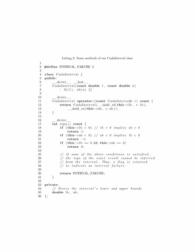
Listing 2: Some methods of our CudaInterval class12 #define INTERVAL_FAILURE 234 class CudaInterval {5 public :6 __device__ __host__7 CudaInterval ( const double l , const double u)8 : lb ( l ) , ub (u) {}9

10 __device__11 CudaInterval operator+(const CudaInterval& v) const {12 return CudaInterval (__dadd_rd( this−>lb , v . lb ) ,13 __dadd_ru( this−>ub , v . ub ) ) ;14 }1516 __device__17 int s i gn ( ) const {18 i f ( this−>lb > 0) // l b > 0 i m p l i e s ub > 019 return 1 ;20 i f ( this−>ub < 0) // ub < 0 i m p l i e s l b < 021 return −1;22 i f ( this−>lb == 0 && this−>ub == 0)23 return 0 ;2425 // I f none o f the above cond i t i on s i s s a t i s f i e d ,26 // the s i gn o f the exac t r e s u l t cannot be i n f e r r e d27 // from the i n t e r v a l , Thus , a f l a g i s re turned28 // to i n d i c a t e an i n t e r v a l f a i l u r e .2930 return INTERVAL_FAILURE;31 }3233 private :34 // Stores the i n t e r v a l ’ s lower and upper bounds35 double lb , ub ;36 } ;

Even though this example is focused on 2D orientation predicates, it canbe extended to other geometric operations using interval arithmetic.

Listing 3: Orientation predicate on GPU1 struct CudaIntervalVertex {2 CudaInterval x , y ;3 } ;45 __device__ int o r i e n t a t i o n (6 const CudaIntervalVertex ∗ p ,7 const CudaIntervalVertex ∗ q ,8 const CudaIntervalVertex ∗ r ) {9 return ( ( q−>x − p−>x) ∗ ( r−>y − p−>y) −

10 (q−>y − p−>y) ∗ ( r−>x − p−>x ) ) . s i gn ( ) ;11 }

4. Fast red–blue intersection tests

We evaluated these ideas by implementing a fast exact algorithm fordetecting red–blue intersections of triangles in 3D. Given T1 red triangles andT2 blue triangles, our objective is to find all the cases where a red triangleintersects a blue triangle. One application is to perform a quick interferencecull between a red object and a blue object, each represented by a union ofoverlapping triangles. Most possible red–blue pairs of objects do not interferewith each other (or intersect). We wish to quickly eliminate most of theimpossibilities, and then spend time on the few hard cases.

In this application, the red object will have many red–red intersections,and the blue object many blue–blue intersections, even if there are no red–blue intersections at all. That is a problem for the classic plane-sweep al-gorithms. They intersect the datasets with a plane and maintain a datastructure describing what objects that plane intersects, and their adjacenciesin that plane. This is used to compute future intersections.

As the plane sweeps up through the data, it stops at each vertex andfuture intersection, and updates its description to reflect adjacency changesand compute more future intersections. It is necessary to stop at all inter-sections, including the red–red and blue–blue ones, in order to update thatdescription.

Even if there are no red–blue intersections, the plane sweep might needto do quadratic work. Our algorithm does not have this problem.

It executes the following series of culls, with each step reducing the num-ber of remaining potential red–blue intersections:

• First, the triangles are indexed using a uniform grid. That is, we iterateover the triangles. For each triangle, all the grid cells that it intersectsare determined, and that information is stored with each such cell.

• Then we interate over the cells. In each cell, we iterate over all the red–blue pairs of triangles, and cull the pairs with a fast bounding-box test.The possible results of each such test are definitely do not intersect, ordon’t know.

• The remaining pairs are next tested with a triangle–triangle intersec-tion algorithm using geometric predicates implemented with intervalarithmetic. The possible results of each such test are definitely inter-sect, definitely do not intersect, or don’t know.

• Finally, the unknown cases are re-evaluated using exact arithmetic.

Details about each step will be presented in the next subsections.

4.1. Uniform Grid IndexingTo avoid testing each triangle from T1 against each one from T2, which

would require quadratic time in the number of triangles, we index the setsusing a uniform grid. This data structure is typically employed in compu-tational geometry to cull a combinatorial set of pairs of objects, generatinga smaller subset with elements that are more likely to coincide [? ]. If theinput is uniformly independent and identically distributed (i.i.d.), the ex-pected size of the resulting subset is linear on the size of the input plus theoutput [? ? 12].

This holds even though some cells might be much more populated thanothers, while many cells remain empty. Indeed, the number of triangles percell is a Poisson random variable. [? ? 12] work this out in detail; it is alsoobserved experimentally. A summary goes as follows.

Let g = r3 be the number of grid cells and n be the number of triangle–cell incidences. An incidence is one occurrence of a triangle intersecting (oroverlapping) one cell. Assume that the triangles are uniformly and indepen-dently distributed over the grid. Although there will be local exceptions tothis, as g, n → ∞ this is reasonable.

Let p be the probability that a given incidence occurs in a given cell.p = 1/g. The expected number of incidences in a given cell is n/g. Let L bethe random variable for the number of incidences in any given cell. L is anexample of combinatorial selection without replacement. Let l be a particularvalue of L. P [L = l] =

(nl

)pl(1− p)n−l. Since E[L] = n/g << n, an excellent

approximation is the Poisson distribution with parameter λ = E[L].If there are l triangles in a cell, the number of pairs of triangles is

(l2

)=

l2

2− l

2. Since for a Poisson distribution, the variance is the square of the

mean, the expected number of pairs of triangles in the cell, which is thetime to process the cell, is on the order of the square of the mean numberof incidences in the cell. With a typical choice of r, the time to process onecell is constant or slowly growing. We might pick r to keep E[L] constant,or sometimes, we might let E[l] grow slowly with dataset size to reduce thespace. Then, the time per cell also grows slowly [? ? 12].

The uniform grid implementation goes as follows. Given the sets of tri-angles T1 and T2, a grid G with resolution r and containing r× r× r cells iscreated covering a box that bounds T1 and T2 together. Next, each trianglet from either of the two input sets is inserted into all the grid cells that t’sbounding-box intersects. Then we iterate over the cells c in G, testing all thepairs of red and blue triangles from each c for intersection. This intersectiontest is the multistep process described earlier. That finds all the pairs ofintersecting triangles.

We implement the uniform grid with a ragged array, similarly to Mag-alhães et al. [? ]. This stores a collection of arrays in a contiguous blockof memory b, by using a dope vector d to keep track of each array’s initialposition. The j-th element of the i-th array is bj+di . Since a ragged arraystores the entire grid in contiguous memory [? ], it is more cache friendly anduses less space than storing one dynamic array per cell. It is also easier totransfer the grid to the GPU. Finally, it parallelizes better than a dynamicarray.

The ragged array is created as follows. First, the triangles are read, thecells intersecting each triangle are computed, and an array k containing thetotal number of triangles intersecting each cell is accumulated.

Then k is transformed into the dope vector d with a parallel prefix-sum,also known as an exclusive scan operation. That is, di =

∑i−1j=0 kj and d0 = 0.

This can be computed in parallel in O(log r) elapsed time, although it’salready so fast, that it doesn’t matter.

t1 t2 t3

t4

t5 t6 t7

t1 t2 t3 t4 t5 t6 t7

Figure 2: Dynamic array versus ragged array - 3 × 3 uniform grid using dynamic arrays(a) versus ragged array (b). Only the memory related to the first row of the grid is shown.Source: [? ]

Finally, the array b is allocated, and the triangles are inserted into it.A counter is kept of the number of triangles that have been inserted so farinto each cell. That can be stored in cells of b that haven’t been used so far.This can mostly be done in parallel. The counter for the number of trianglesin each cell has to be read and incremented atomically. However, when thenumber of cells is much more than the number of threads, collisions are rare.

Figure 2 illustrates the indexing of a mesh using a 2D uniform grid builtwith a dynamic array 2(a), and a ragged array 2(b).

4.2. Bounding-box CullingFor large datasets, depending on r, there may be many triangles in each

cell. In each cell, we will doubly iterate through the red and the blue triangles,testing each red–blue pair for intersection. Before the exact test, we use abounding box cull, since it is much faster than the exact test, and it eliminatesmany pairs that do not intersect.

Doing this correctly requires care. However that is necessary becausean incorrectly determined intersection might cause topological errors whenthis algorithm is a subroutine in a bigger algorithm such as determining allthe intersection information about intersecting two meshes, in addition tojust the intersecting triangles. The key is that, whenever a coordinate of abounding box is approximated, to round it in the direction of making thebox bigger.

The bounding-box filtering can be done on the GPU with two passes. Inthe first pass, the number of pairs whose bounding-boxes intersect each otheris counted. Each thread is responsible for checking one pair of triangles. Iftheir bounding-boxes overlap, the thread increments a counter (stored in theGPU global memory) via an atomic add operation (atomicAdd) . We will

show in the experiments that the synchronized operation does not imposea significant performance overhead. If this step were a bottleneck, it couldbe improved with a more sophisticated reduction operation using a fastermemory from the hierarchy.

The counter is returned to the CPU, which then allocates an array to holdall the pairs whose bounding-boxes do overlap, and so have to be tested forintersection. The algorithm then proceeds to the second pass, and the GPUis now responsible for populating this array. Each thread processes again onepair of triangles, and if their bounding-boxes overlap, the thread inserts itspair into the array. The insertion is performed by employing another globalcounter (initially set to 0), which is also incremented employing the thread-safe atomicAdd operation. This operation returns the value of the variable,and then increments it. This ensures each thread will insert a triangle intoa different position of the array.

To perform these passes, the pairs that each thread will process haveto be carefully selected. Traversing the grid to create an array of pairs sothat each GPU thread would be responsible for processing a pair can beunfeasible, as shown in our previous work [? ]. In order to avoid this costlypre-processing step, an approach for implicitly associating a thread with apair will be employed.

4.3. Implicit Thread AssociationIn [? ] we presented three techniques for delegating work to be done by

the GPU threads when there are many pairs of objects in a uniform grid.The focus of that work was on intersecting segments against triangles, butthis delegation strategy can also be applied for the current problem.

In this paper we will employ the method with the best performance tolaunch the threads in the two bounding-box filtering passes on the GPU).This subsection will describe this technique (details are available in [? ]).

The idea is to launch the thread blocks such that threads in the sameblock will always process the same uniform grid cell. Let T1c and T2c be thenumber of triangles in meshes T1 and T2, respectively that are contained inthe uniform grid cell c. If the algorithm is configured to launch Tc threadsper CUDA block,

⌈T1c×T2c

Tc

⌉blocks will have to be launched to completely

process the pairs of triangles in c.The following three arrays are created in order for each thread to deter-

mine which pair of triangles it is responsible for processing. For simplicity,these arrays are initially created on the CPU and then copied to the GPU:

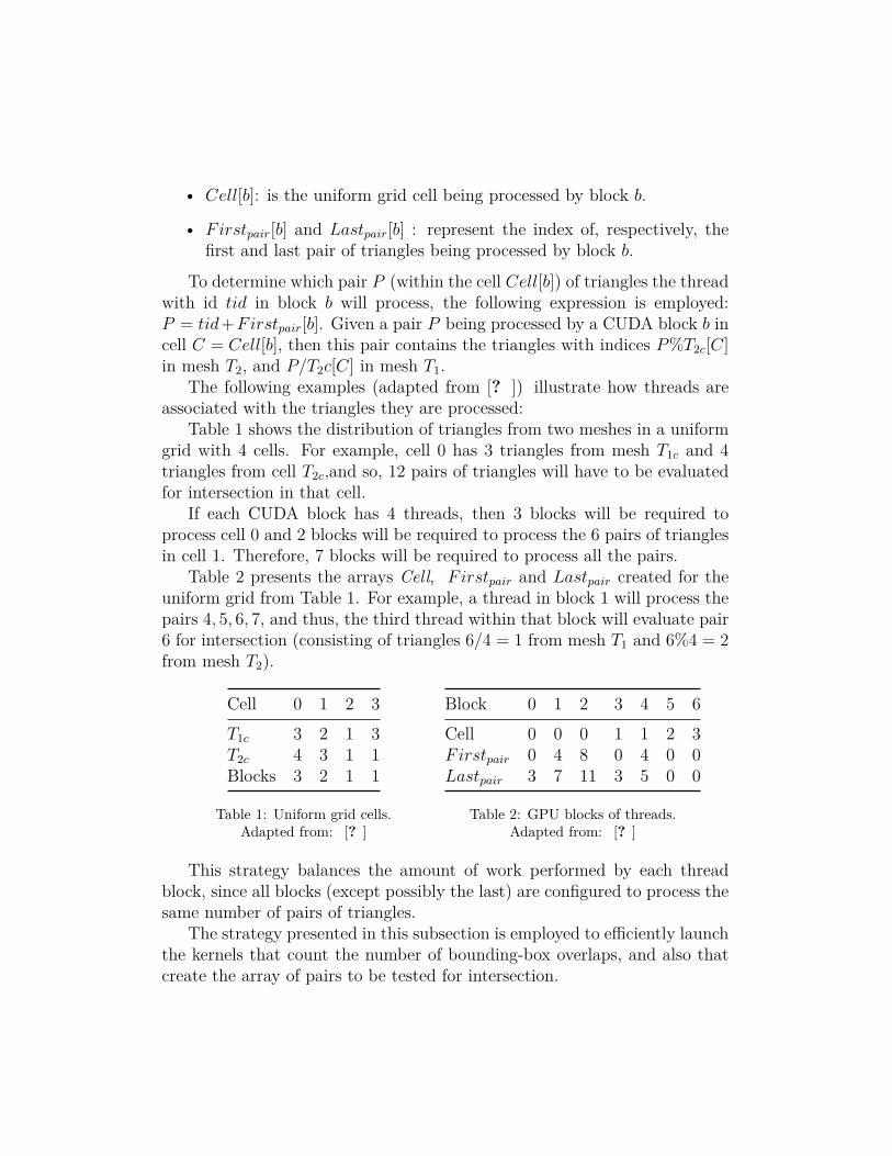
• Cell[b]: is the uniform grid cell being processed by block b.

• Firstpair[b] and Lastpair[b] : represent the index of, respectively, thefirst and last pair of triangles being processed by block b.

To determine which pair P (within the cell Cell[b]) of triangles the threadwith id tid in block b will process, the following expression is employed:P = tid+Firstpair[b]. Given a pair P being processed by a CUDA block b incell C = Cell[b], then this pair contains the triangles with indices P%T2c[C]in mesh T2, and P/T2c[C] in mesh T1.

The following examples (adapted from [? ]) illustrate how threads areassociated with the triangles they are processed:

Table 1 shows the distribution of triangles from two meshes in a uniformgrid with 4 cells. For example, cell 0 has 3 triangles from mesh T1c and 4triangles from cell T2c,and so, 12 pairs of triangles will have to be evaluatedfor intersection in that cell.

If each CUDA block has 4 threads, then 3 blocks will be required toprocess cell 0 and 2 blocks will be required to process the 6 pairs of trianglesin cell 1. Therefore, 7 blocks will be required to process all the pairs.

Table 2 presents the arrays Cell, Firstpair and Lastpair created for theuniform grid from Table 1. For example, a thread in block 1 will process thepairs 4, 5, 6, 7, and thus, the third thread within that block will evaluate pair6 for intersection (consisting of triangles 6/4 = 1 from mesh T1 and 6%4 = 2from mesh T2).

Cell 0 1 2 3

T1c 3 2 1 3T2c 4 3 1 1Blocks 3 2 1 1

Table 1: Uniform grid cells.Adapted from: [? ]

Block 0 1 2 3 4 5 6

Cell 0 0 0 1 1 2 3Firstpair 0 4 8 0 4 0 0Lastpair 3 7 11 3 5 0 0

Table 2: GPU blocks of threads.Adapted from: [? ]

This strategy balances the amount of work performed by each threadblock, since all blocks (except possibly the last) are configured to process thesame number of pairs of triangles.

The strategy presented in this subsection is employed to efficiently launchthe kernels that count the number of bounding-box overlaps, and also thatcreate the array of pairs to be tested for intersection.

The other strategies evaluated in [? ] presented challenges such as loadunbalancing. For example, if each CUDA thread was configured to processone triangle t from T1 and test it for intersection against triangles from T2 inthe same uniform grid cells as t, the varying number of triangles in each cellcould create thread divergence and load unbalance.

4.4. Intersection evaluationThe main step of the algorithm is evaluating intersection predicates with

interval arithmetic. After the uniform grid indexing and bounding-box culling,the result is an array (already located on the GPU) of potentially intersectingtriangle pairs. These pairs are then tested for intersection.

Two additional arrays are allocated in the GPU (with the same size asthe array of pairs) in order to store the pairs of triangles that intersect, andalso the ones that resulted in interval failures.

After the arrays are allocated, a GPU kernel is launched to test the pairsfor intersection. Each thread evaluates the intersection of a pair of triangles(t1,t2), using five 3D orientation predicates in order to verify if any edge oft1 intersects t2 (and vice-versa) [17].

The intersecting pairs (and the ones whose intersections resulted in in-terval failures) are inserted into the resulting arrays by employing a globalcounter for each array, using thread-safe atomicAdd operations.

A triangle may overlap, and so be inserted into, two or more differentuniform grid cells. Therefore one pair of triangles may be tested for inter-section more than once, causing duplicates in the intersections array. Theseduplicates are removed in the next step.

4.5. Eliminating Duplicates and Performing Exact Re-evaluationThe resulting arrays of intersecting pairs of triangles and interval failures

are sorted on the GPU with a parallel radix-sort, and then the duplicates areremoved. This uses sort and unique from the Thrust library [10]. (Whenthe sort key is a plain old datatype (POD), the radix sort takes time linear inthe number of records being sorted. It also reads and writes in a predictablepattern. Both properties contrast favorably to the widely used quicksort.)The sorted arrays are then copied back to the CPU for possible future useby other algorithms.

In the next step, the array containing the pair of triangles whose inter-section computation resulted in interval failures is exactly re-evaluated onthe CPU in parallel using OpenMP. Each pair is evaluated using the same

predicates that were used on the GPU. However this time, the computation isperformed with arbitrary precision rational numbers instead of floating-pointintervals.

If the intervals are implemented using single-precision floating-point num-bers, the post-processing time can be reduced by re-evaluating the arithmeticfailures with double-precision, and then using the rationals only for the pred-icates that also led to failures with doubles. This idea of re-evaluating pred-icates with increasing precision in geometric predicates has been previouslyapplied, for example, by Shewchuck [18].

The intersections detected in this step are then appended to the onesdetected on the GPU.

4.6. Algorithm complexityThe complexity of the bounding-box culling step is O(r3 +Bt), where r3

is the number of cells (for an uniform grid resolution r) and Bt is the totalnumber of bounding-box tests in all grid cells.

From Section 4.1, Bt is expected to be linear in the size of the input plusthe number of intersecting bounding-boxes. Thus, Bt = O(T1 + T2 + I),where T1 and T2 is the number of triangles in the input meshes and I is thenumber of intersecting bounding boxes in all grid cells.

In the worst case, the intersection tests and post-processing steps willhave a time complexity O(I) since the parallel sort in the post-processingstep is linear complexity, and the number of operations performed on eachpair of triangles is constant.

Therefore, the total time and space complexity of the algorithm are bothO(r3 + T1 + T2 + I). The resolution of the grid (r) is a small constant tunedby the user to achieve a small number of triangles per cell while keeping thenumber of duplicate bounding boxes in the grid small. That way, I is linearon the number of unique intersecting bounding boxes.

An adversary could create hard test cases where all the triangles in thetwo input meshes are equal, or every bounding-box intersects every cell. Theneach triangle will be in all r3 cells, and thus, I = O(r3 × T1 × T2), while thenumber of unique intersections is O(T1 × T2). However, bad test cases couldalso be created for other algorithms, such as the plane-sweep. Finally, thisdoes not affect our parallel speedup, since the number of intersection testswould be equal to the one in the sequential algorithm.

Mesh name Mesh id # vertices # triangles

OpenToys 914686 66 166 605 279GreatSkull 260537 67 265 664 101Pegasus 68380 106 955 1 066 547Armadillo - 340 043 3 377 086Lampan 518092 603 116 5 937 604BioInteractive 461112 841 883 8 494 878

Table 3: Number of vertices and triangles in the meshes employed in the experiments.The mesh id can be used to locate the ones downloaded from the Thingi10K website.

5. Experiments

The fast algorithm for intersecting triangles was implemented in C++and CUDA. It was evaluated on a dual Intel Xeon E5-2660 CPU at 2 GHz(3.2GHz Turbo Boost), with 256 GB of RAM and a NVIDIA Quadro RTX8000 GPU. Arbitrary-precision arithmetic was provided by the GMP li-brary [7].

We always used a uniform grid of size 100×100×100. However, there areheuristics for automatically choosing a grid resolution basing on statistics ofthe input datasets [? ? ], such as choosing the grid size make the expectednumber of edges per cell a constant. As shown by Magalhães et al. [? ], therange of grid configurations with reasonable performance optimum is broad.This follows because a finer grid causes one part of the algorithm to run morequickly and another part to run more slowly.

We performed experiments on meshes from two public repositories. TheArmadillo mesh was downloaded from the Stanford repository [20] and theother ones were downloaded from Thingi10K [? ]. These meshes were firsttetrahedralized using GMSH [6]. Table 3 describes the dataset and Fig-ure 3 illustrates it. These datasets’ sizes ranged from 600K to 8M triangles.Figure 4 shows the interior of mesh OpenToys after tetrahedralization, andFigure 5 shows two overlaid pairs of meshes employed in the experiments.

In contrast to CPUs, GPUs typically have significantly more single-precisionfloating point units than double-precision (since they focus on applicationswhere the lower precision of floats is acceptable) [? ]. For example, the RTX8000 GPU employed in these experiments has a peak single and double-precision performance of, respectively, 16 TFLOPS and 0.5 TFLOPS. Thus

(a) Armadillo (b) OpenToys

(c) GreatSkull (d) Pegasus

(e) Lampan (f) BioInteractive

Figure 3: Meshes employed in the experiments.

Figure 4: Mesh OpenToys (left). The right figure illustrates its tetrahedralized interior(Source: [? ]).

(a) (b)

Figure 5: Examples of pairs selected for intersection tests. (a) Armadillo (red) and Ar-madilloTranslated (white) (b) GreatSkull (red) and OpenToys (white).

we also implemented a version of the GPU code employing intervals withsingle-precision floats. As described in Section 4.5, the single-precision arith-metic failures were re-evaluated with double-precision intervals, and finallyonly if necessary were re-evaluated with rationals.

The following listing contains the 3 implementations evaluated in theexperiments:

• CPU : sequential CPU implementation employing arithmetic filters us-ing double-precision intervals (provided by the CGAL Interval_nt class [3]).This is the baseline implementation.

• GPUDouble: parallel GPU implementation using double-precision in-tervals implemented as described in this paper.

• GPUFloat: the same implementation as GPU double, but with single-precision floats in the intervals.

5.1. Experiments on the RTX 8000 GPUTables 4 and 5 present the results of intersecting pairs of triangles from

the input meshes. We assume the uniform grid index is already created asa ragged-array and loaded in the CPU memory.

Separate times were measured for pre-processing, intersection, post-processing,and data transfer.

The pre-processing includes accessing the index and performing bounding-box tests to cull the number of triangles actually tested for intersection. Forthe GPU implementation, the time for processing the uniform grid to dis-tribute the work to the threads (as described in Section 4.3) is also included(see Section 4.3).

The intersection is the time spent evaluating pairs of triangles for intersec-tion using interval arithmetic. In the current implementation, our algorithmonly reports nondegenerate intersections.

Special cases (such as two triangles intersecting at a single point), whichhappen when at least one of the orientation predicates returns 0, could behandled by flagging these cases and re-evaluating them on the CPU duringthe post-processing. Indeed, interval arithmetic would typically lead to in-terval failures in these cases because the sign of the interval of a determinantthat is equal to 0 cannot be reliably determined (since floating-point errorswill usually cause its bounds not to be both 0). This is not a limitation ofthe proposed technique for two reasons: first, this affects other algorithms

based on interval arithmetic, and second, as will be shown in the experiments,the number of intersection tests is typically much larger than the number ofintersections.

Post-processing includes sorting the pairs of intersecting triangles to re-move duplicates, and then re-evaluating, on the CPU, the computationswhose intervals failed.

The data transfer is the total time for transferring the input, intermediateand output data between the CPU and GPU.

Finally, the last four rows of each table include the number of bounding-box tests performed by the algorithm (including duplicates), the number ofunique bounding-box tests , the number of intersection tests (i.e., the numberof pairs of triangles whose bounding-boxes do intersect) and the number ofintersections.

In the CPU version of the algorithm, the bottleneck in all cases was test-ing pairs of triangles for intersection using interval arithmetic. In this step,GPUDouble achieved a speedup ranging from 50× to 63×, while GPUFloatachieved up to 1936× of speedup. This performance difference is consistentwith the difference in the peak single and double precision floating-pointcomputing powers of the RTX 8000 GPU.

The good performance of the GPU algorithms in this step can be ex-plained because they are compute-intensive, using 3D vector operations suchas subtraction and mixed-product.

In all tests with GPUFloat, the bottleneck was the data transfer. Morethan 80% of the total data transfer time was used for initially sending the uni-form grid, the triangles and the auxiliary arrays used for the implicit threadassociation to the GPU. Indeed, excluding the data transfers, the best to-tal speedup would have been 731× instead of 414×. Thus, applications notrequiring frequent data transfer between the CPU and GPU could benefiteven further from our method. Also, if processing many datasets simulta-neously, one job’s data transfer could occur concurrently with another job’scomputation, perhaps using CUDA streams.

The worst total speedup of GPUFloat was 127×, with the Armadillodatasets. This step had the lowest percentage of pairs of triangles (selectedby the index) whose bounding-boxes do intersect. Indeed, only 21% of thepairs of bounding-boxes filtered by the uniform grid do intersect, as opposedto 55%, 58% and 77% (the best total speedup) in the other test cases. As aresult, in this dataset 21% of the pairs of triangles selected at the indexingstep reached the intersection computation step (the most time-consuming

Dataset GreatSkull vs OpenToys

Method: CPU GPUDouble GPUFloat

Time (s) Time (s) Speedup Time (s) Speedup

Pre-processing 1.13 0.05 25 0.05 25Intersection 55.59 1.09 51 0.04 1496Post-processing 0.89 0.02 51 0.03 30Data transfer - 0.14 - 0.14 -Total time 57.62 1.29 45 0.25 232

#bounding-box tests 109.1× 106

#unique bounding-box tests 33.5× 106

#intersection tests 59.5× 106

#intersections 2.2× 106

Dataset Pegasus vs OpenToys



Pre-processing 1.73 0.07 24 0.07 25Intersection 81.59 1.63 50 0.05 1579Post-processing 1.40 0.04 31 0.04 33Data transfer - 0.25 - 0.24 -Total time (s) 84.71 2.00 42 0.41 208





Table 4: Times (in seconds) spent by the the intersection tests between meshes GreatSkullvs OpenToys and Pegasus vs OpenToys. Speedup shows the speedup of the correspondingGPU version of the algorithm when compared against the CPU one.

Dataset Armadillo vs ArmadilloTranslated








Dataset BioInteractive vs Lampan








Table 5: Times (in seconds) spent by the the intersection tests between meshes Armadillovs ArmadilloTranslated and BioInteractive vs Lampan. Speedup shows the speedup of thecorresponding GPU version of the algorithm when compared against the CPU one.

one in the CPU and the one with the best parallel speedup), which reducesthe total speedup.

The two GPU implementations had similar performance in the datatransfer and pre-processing steps (in the worst case GPUDouble was 10%slower than GPUFloat). The higher post-processing time of GPUFloat canbe explained because of the lower precision of floats, which leads to moreinterval failures, requiring more intersections to be re-evaluated with doublesand rationals on the CPU.

In the experiments intersecting meshes BioInteractive and Lampan, forexample, the post-processing time of 0.05s for GPUFloat was composed of0.011s for sorting the resulting intersections and removing duplicates, 0.003sfor filtering the pairs of triangles whose intersection computations had in-terval failures and 0.039s for re-evaluating the interval failures with doubles.In this experiment, only 0.01% of the intersection tests led to failures andthe results with double precision were computed successfully (thus, rationalswere not necessary). GPUDouble and CPU, on the other hand, had no filterfailures and, thus, only spent time sorting the results to remove duplicates.

The number of pairs of bounding-boxes evaluated for intersection wasfrom 1.6 to 3.4 times larger than the number of unique pairs. These duplicatesare not removed at the beginning of the algorithm because, as mentionedin Section 4.3, the list of pairs is implicitly created by the threads. Sincethe performance bottleneck is data transfer and these duplicates are nevertransferred to the CPU, this did not significantly affect the efficiency of thealgorithm.

Over all the experiments, in the worst case (intersection of meshes Pegasusand OpenToys), only 0.001 % of the intersection tests had to be performedwith rationals.

Table 6 compares the 3 implementations against versions without thebounding-box culling. As can be seen, detecting intersections was 80%, 86%and 25% slower when no bounding-box filtering was performed in, respec-tively, the CPU, GPUDouble and GPUFloat methods, while there was nosignificative difference in the other steps. As shown in Tables 4 and 5, inthis test case, the number of intersection tests when no bounding-box filteringis employed was 83% larger (109× 106 versus 59.5× 106).

5.2. Experiments on a lower-end computerWe also performed experiments on another computer with an NVIDIA

1070 Ti GPU (8 GB of RAM), AMD Ryzen 5 1600 CPU 3.2 GHz (12 hy-

Dataset GreatSkull vs OpenToysMethod CPU CPU* GPUD. GPUD.* GPUF. GPUF.*

Pre-processing 1.13 1.14 0.05 0.04 0.05 0.04Intersection 55.59 100.50 1.09 2.03 0.04 0.05Post-processing 0.89 0.90 0.02 0.02 0.03 0.04data transfer - - 0.14 0.14 0.14 0.14Total time 57.62 102.54 1.29 2.22 0.25 0.26

Table 6: Times (in seconds) spent by the different versions of the algorithms for intersectinga particular pair of meshes. The methods labeled with * do not employ a bounding-box culling. GPUD. and GPUF. represent, respectively, the GPUDouble and GPUFloatmethods.

perthreads), 16GB of RAM in order to evaluate the proposed technique ona lower-end GPU. Table 7 presents the results for a pair of meshes. Thebiggest difference was in the intersection step, whose time increased from0.05s to 0.20s compared to the time on the RTX 8000 GPU. Because of thedata transfer operations and sequential steps of the algorithm, the differencein the total running-time (for GPUFloat) is smaller (the total time increasedfrom 0.41s to 0.54s on the lower-end GPU).

Even though, as expected, the running-time on the lower-end GPU ishigher than on the RTX 8000 GPU, the performance difference when com-pared against the CPU implementation is still high. For example, GPUFloatachieved speedups of, respectively, 407× and 158× for the intersection andtotal times when compared against CPU.

6. Conclusions and future work

We proposed the use of GPUs to accelerate the evaluation of exact geo-metric predicates filtered with intervals of floating-point numbers. The ideais to evaluate the predicates using interval arithmetic on the GPU. The fewresults that could not be guaranteed to be correct are then re-evaluated onthe CPU using arbitrary-precision rationals.

As a proof of concept, a parallel algorithm for detecting intersections ofred and blue triangles has been implemented. Because of the high computingpower of the GPU for processing floating-point numbers, a speedup of up to1936 times (when compared against the sequential version) was obtained in

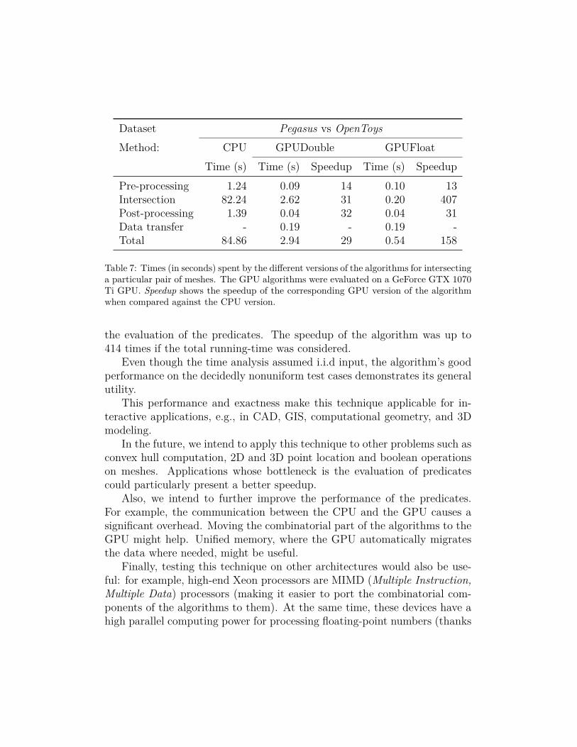
Dataset Pegasus vs OpenToysMethod: CPU GPUDouble GPUFloat


Pre-processing 1.24 0.09 14 0.10 13Intersection 82.24 2.62 31 0.20 407Post-processing 1.39 0.04 32 0.04 31Data transfer - 0.19 - 0.19 -Total 84.86 2.94 29 0.54 158

Table 7: Times (in seconds) spent by the different versions of the algorithms for intersectinga particular pair of meshes. The GPU algorithms were evaluated on a GeForce GTX 1070Ti GPU. Speedup shows the speedup of the corresponding GPU version of the algorithmwhen compared against the CPU version.

the evaluation of the predicates. The speedup of the algorithm was up to414 times if the total running-time was considered.

Even though the time analysis assumed i.i.d input, the algorithm’s goodperformance on the decidedly nonuniform test cases demonstrates its generalutility.

This performance and exactness make this technique applicable for in-teractive applications, e.g., in CAD, GIS, computational geometry, and 3Dmodeling.

In the future, we intend to apply this technique to other problems such asconvex hull computation, 2D and 3D point location and boolean operationson meshes. Applications whose bottleneck is the evaluation of predicatescould particularly present a better speedup.

Also, we intend to further improve the performance of the predicates.For example, the communication between the CPU and the GPU causes asignificant overhead. Moving the combinatorial part of the algorithms to theGPU might help. Unified memory, where the GPU automatically migratesthe data where needed, might be useful.

Finally, testing this technique on other architectures would also be use-ful: for example, high-end Xeon processors are MIMD (Multiple Instruction,Multiple Data) processors (making it easier to port the combinatorial com-ponents of the algorithms to them). At the same time, these devices have ahigh parallel computing power for processing floating-point numbers (thanks

to wide Single Instruction, Multiple Data - SIMD instructions in the individ-ual cores). Thus, we believe both algorithms and exact geometric predicatescould be accelerated on these devices using these instructions (keeping bothin the same device would reduce the communication overhead).

7. Acknowledgement

This research was partially supported by CAPES, FAPEMIG and FU-NARBE.

References

[1] Samuel Audet, Cecilia Albertsson, Masana Murase, and Akihiro Asa-hara. 2013. Robust and Efficient Polygon Overlay on Parallel StreamProcessors. In Proceedings of the 21st ACM SIGSPATIAL Interna-tional Conference on Advances in Geographic Information Systems(SIGSPATIAL’13). ACM, New York, NY, USA, 304–313. https://doi.org/10.1145/2525314.2525352

[2] Alberto Belussi, Sara Migliorini, Mauro Negri, and Giuseppe Pelagatti.2016. Snap Rounding with Restore: An Algorithm for Producing RobustGeometric Datasets. ACM Trans. Spatial Algorithms and Syst. 2, 1,Article 1 (March 2016), 36 pages. https://doi.org/10.1145/2811256

[3] CGAL. 2018. Computational Geometry Algorithms Library. (2018).Retrieved 2018-09-09 from https://www.cgal.org

[4] Mark de Berg, Dan Halperin, and Mark Overmars. 2007. Anintersection-sensitive algorithm for snap rounding. Computational Ge-ometry 36, 3 (Apr. 2007), 159–165.

[5] European Space Agency. [n. d.]. Ariane 501 Inquiry Board Report. ([n.d.]). http://ravel.esrin.esa.it/docs/esa-x-1819eng.pdf (retrieved on Jun-2015).

[6] Christophe Geuzaine and Jean-François Remacle. 2009. Gmsh: A 3-D finite element mesh generator with built-in pre-and post-processingfacilities. Int. J. for Numerical Methods in Eng. 79, 11 (May 2009),1309–1331. https://doi.org/10.1002/nme.2579

[7] Torbjorn Granlund and the GMP development team. 2014. GNU MP:The GNU Multiple Precision Arithmetic Library (6.0.0 ed.). http://gm-plib.org/ (retrieved on Jun-2015).

[8] John Hershberger. 2013. Stable snap rounding. Comput. Geom. 46, 4(May 2013), 403–416.

[9] John D. Hobby. 1999. Practical segment intersection with finite pre-cision output. Comput. Geom. 13, 4 (1999), 199–214. http://dblp.uni-trier.de/db/journals/comgeo/comgeo13.html\#Hobby99

[10] Jared Hoberock and Nathan Bell. 2010. Thrust: A Parallel TemplateLibrary. (2010). http://thrust.github.io/ Version 1.7.0.

[11] Christoff M. Hoffman. 1989. The Problems of Accuracy and Robustnessin Geometric Computation. Computer 22, 3 (1989), 31–40. https://doi.org/10.1109/2.16223

[12] Sara Hopkins and Richard G. Healey. 1990. A Parallel Implementationof Franklin’s Uniform Grid Technique for Line Intersection Detection ona Large Transputer Array. In 4th International Symposium on SpatialData Handling, Kurt Brassel and H. Kishimoto (Eds.). Zürich, 95–104.

[13] Alec Jacobson, Daniele Panozzo, et al. 2016. libigl: A Simple C++Geometry Processing Library. (2016). Retrieved 2017-10-18 from http://libigl.github.io/libigl/

[14] Lutz Kettner, Kurt Mehlhorn, Sylvain Pion, Stefan Schirra, and CheeYap. 2008. Classroom Examples of Robustness Problems in GeometricComputations. Comput. Geom. Theory Appl. 40, 1 (May 2008), 61–78.https://doi.org/10.1016/j.comgeo.2007.06.003

[15] Chen Li, Sylvain Pion, and Chee-Keng Yap. 2005. Recent progressin exact geometric computation. The Journal of Logic and AlgebraicProgramming (2005), 85–111.

[16] Sylvain Pion and Andreas Fabri. 2011. A generic lazy evaluation schemefor exact geometric computations. Sci. Comput. Program. 76, 4 (Apr.2011), 307 – 323.

[17] Rafael Jesús Segura and Francisco R. Feito. 2001. Algorithms to TestRay-Triangle Intersection. Comparative Study. In The 9-th Int. Conf.Central Europe Comput. Graph., Visualization Comput. Vision’2001,WSCG 2001. 76–81.

[18] Jonathan Richard Shewchuk. 1997. Adaptive Precision Floating-PointArithmetic and Fast Robust Geometric Predicates. Discret. & Comput.Geom. 18, 3 (Oct. 1997), 305–363.

[19] R. Skeel. [n. d.]. Roundoff Error and the Patriot Missile. SIAM News25 ([n. d.]). Jul. 1992.

[20] Stanford Scanning Repository 2016. The Stanford 3D Scanning Reposi-tory. (2016). Retrieved 2016-02-02 from http://graphics.stanford.edu/data/3Dscanrep/

Fastparallelevaluationofexactgeometricpredicateson GPUs

Documents

Transcript of Fastparallelevaluationofexactgeometricpredicateson GPUs