1

FastCam

Operation Manual by

Rafael Barrena & the FastCam Team(1)

Last revision: November 2010

(1) See www.iac.es/proyecto/fastcam/

2

Table of Contents 1. Introduction ................................................................................................................ 3

2. Control computers ...................................................................................................... 5

3. Observing sequence .................................................................................................... 6

4. Startup ......................................................................................................................... 7

5. Camera Operation ...................................................................................................... 7

5.1 Andor Camera Setup ........................................................................................... 8

5.2 Changing filters .................................................................................................... 9

5.3 Bias and flat-fields .............................................................................................. 10

5.4 Telescope control from FastCam ...................................................................... 10

6. Data saving and processing...................................................................................... 11

7. Exploring the reduced images ................................................................................. 14

8. Shutting down ........................................................................................................... 15

9. Some recommendations ........................................................................................... 15

9.1 Finding the right gain exposure time ................................................................ 15

9.1.1 How to use FastCam for long exposures ................................................... 16

9.2 Aligning FOVIA and FastCam.......................................................................... 16

9.3 Focusing the telescope ........................................................................................ 16

9.4 Pixel Scale and field orientation ........................................................................ 17

9.5 Atmospheric dispersion effects.......................................................................... 17

10. Frequent problems ................................................................................................. 17

11. References................................................................................................................ 18

Appendix A. On the EM gain ...................................................................................... 19

Appendix B. On the detector linearity........................................................................ 19

Appendix C. “ImageJ tasks”, a secondary software to process fastcam data cubes

........................................................................................................................................ 20

3

1. Introduction

FastCam (http://www.iac.es/proyecto/fastcam/) is an instrument jointly developed by

the Spanish Instituto de Astrofísica de Canarias and the Universidad Politécnica de

Cartagena, designed to obtain high spatial resolution images in the optical wavelength

range from ground-based telescopes.

The instrument consists of a very low noise and very fast readout speed EMCCD

camera capable of reaching the diffraction limit of medium-sized telescopes from 500 to

850 nm. The undisturbed images represent a small fraction of the observations.

Therefore, a special software package has been developed to extract, from cubes of tens

of thousands of images, those with better quality than a given level, following the

“lucky imaging” technique (see, e.g., Tubbs et al. 2003; Law, Mackay & Baldwin

2006). This is done in parallel with the data acquisition at the telescope.

The project started in March 2006 and, since then, FastCam has been successfully tested

in four telescopes: the 1.52-meter Telescopio Carlos Sánchez (TCS, Teide

Observatory), the 2.5-meter NOT, the 4.2-meter WHT and the 10.4m GTC telescope

(Roque de los Muchachos Observatory). The theoretical diffraction limit of the first

three telescopes has been reached in the I band (850 nm) -0.15, 0.09 and 0.06 arcsec,

respectively-, and similar resolutions have been also obtained in the V and R bands.

Figure 1. FastCam Optomechanics mounted at the Cassegrain focus of

the Carlos Sanchez telescope.

FastCam is, since September 2008, a common-user instrument at the Cassegrain focus

of the TCS. The instrument makes use of an Andor iXon DU-897 back-illuminated

system containing a 512x512 pixel frame transfer CCD sensor from E2V Technologies.

The pixel size is 16 micron and the DU-897 camera allows up to 30 exposures per

second.

4

Figure 2. FastCam system interconnection overview.

The image selection technique known as lucky imaging is based on the idea of

registering the instants of atmospheric stability, typically lasting just some milliseconds,

using very short exposures. The selection of only those images minimally affected by

turbulence allows the system to reach the resolution limit in the optical range, i.e. offers

to ground-based telescopes the possibility of obtaining resolutions similar to those of

space telescopes. This idea was originally presented by D. L. Fried (1979), who called

lucky images those exposures taken under minimum turbulence conditions.

Figure 3. Series of 30 ms images of the star GJ 436 taken with the

TCS. The PSF distortion due to the atmosphere can be seen with very

short exposures, generating Speckle patterns, i.e. sets of small spots

with the size of the telescope’s resolution limit and containing the

information of the star before its distortion. The field of view is of 6”

with a 2.2” seeing and a pixel size of 76mas/px.

5

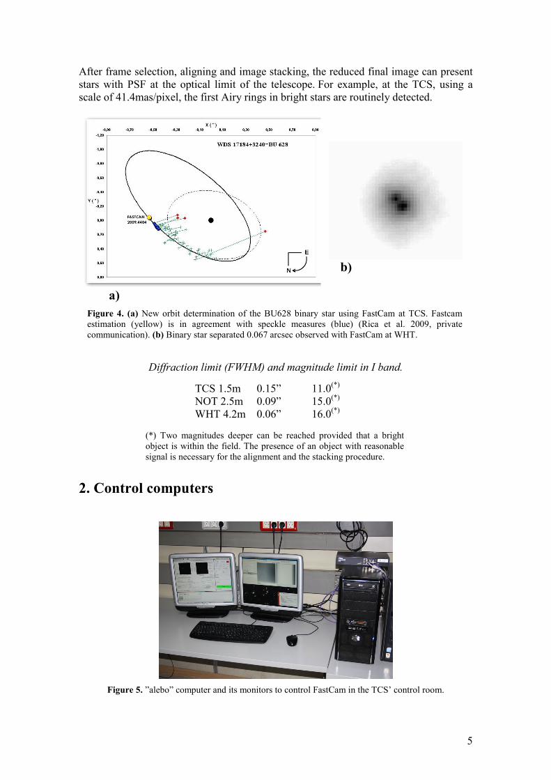
After frame selection, aligning and image stacking, the reduced final image can present

stars with PSF at the optical limit of the telescope. For example, at the TCS, using a

scale of 41.4mas/pixel, the first Airy rings in bright stars are routinely detected.

a)

b)

Figure 4. (a) New orbit determination of the BU628 binary star using FastCam at TCS. Fastcam

estimation (yellow) is in agreement with speckle measures (blue) (Rica et al. 2009, private

communication). (b) Binary star separated 0.067 arcsec observed with FastCam at WHT.

Diffraction limit (FWHM) and magnitude limit in I band.

TCS 1.5m 0.15” 11.0(*)

NOT 2.5m 0.09” 15.0(*)

WHT 4.2m 0.06” 16.0(*)

(*) Two magnitudes deeper can be reached provided that a bright

object is within the field. The presence of an object with reasonable

signal is necessary for the alignment and the stacking procedure.

2. Control computers

Figure 5. ”alebo” computer and its monitors to control FastCam in the TCS’ control room.

6

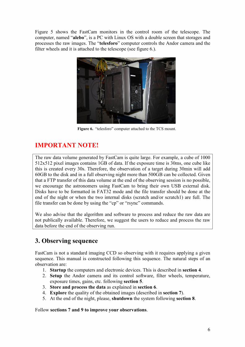
Figure 5 shows the FastCam monitors in the control room of the telescope. The

computer, named “alebo”, is a PC with Linux OS with a double screen that storages and

processes the raw images. The “telesforo” computer controls the Andor camera and the

filter wheels and it is attached to the telescope (see figure 6.).

Figure 6. “telesforo” computer attached to the TCS mount.

IMPORTANT NOTE!

The raw data volume generated by FastCam is quite large. For example, a cube of 1000

512x512 pixel images contains 1GB of data. If the exposure time is 30ms, one cube like

this is created every 30s. Therefore, the observation of a target during 30min will add

60GB to the disk and in a full observing night more than 500GB can be collected. Given

that a FTP transfer of this data volume at the end of the observing session is no possible,

we encourage the astronomers using FastCam to bring their own USB external disk.

Disks have to be formatted in FAT32 mode and the file transfer should be done at the

end of the night or when the two internal disks (scratch and/or scratch1) are full. The

file transfer can be done by using the “cp” or “rsync” commands.

We also advise that the algorithm and software to process and reduce the raw data are

not publically available. Therefore, we suggest the users to reduce and process the raw

data before the end of the observing run.

3. Observing sequence

FastCam is not a standard imaging CCD so observing with it requires applying a given

sequence. This manual is constructed following this sequence. The natural steps of an

observation are:

1. Startup the computers and electronic devices. This is described in section 4. 2. Setup the Andor camera and its control software, filter wheels, temperature,

exposure times, gains, etc. following section 5.

3. Store and process the data as explained in section 6. 4. Explore the quality of the obtained images (described in section 7). 5. At the end of the night, please, shutdown the system following section 8.

Follow sections 7 and 9 to improve your observations.

7

4. Startup

If all computers are off, please follow the next steps to startup the system (although this

should be done by the night assistant):

1. Switch the instrument on, connecting it to the 220AC red switches just behind the mirror of the telescope.

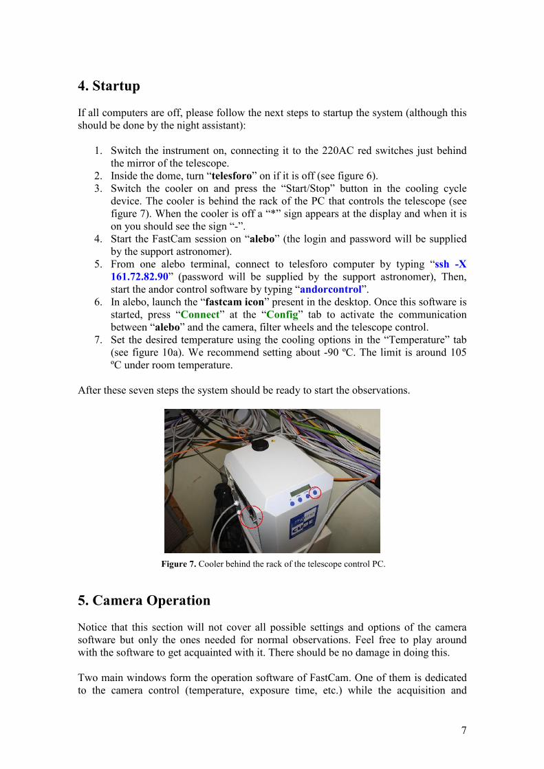
2. Inside the dome, turn “telesforo” on if it is off (see figure 6). 3. Switch the cooler on and press the “Start/Stop” button in the cooling cycle

device. The cooler is behind the rack of the PC that controls the telescope (see

figure 7). When the cooler is off a “*” sign appears at the display and when it is

on you should see the sign “-”.

4. Start the FastCam session on “alebo” (the login and password will be supplied by the support astronomer).

5. From one alebo terminal, connect to telesforo computer by typing “ssh -X 161.72.82.90” (password will be supplied by the support astronomer), Then,

start the andor control software by typing “andorcontrol”.

6. In alebo, launch the “fastcam icon” present in the desktop. Once this software is started, press “Connect” at the “Config” tab to activate the communication

between “alebo” and the camera, filter wheels and the telescope control.

7. Set the desired temperature using the cooling options in the “Temperature” tab (see figure 10a). We recommend setting about -90 ºC. The limit is around 105

ºC under room temperature.

After these seven steps the system should be ready to start the observations.

Figure 7. Cooler behind the rack of the telescope control PC.

5. Camera Operation

Notice that this section will not cover all possible settings and options of the camera

software but only the ones needed for normal observations. Feel free to play around

with the software to get acquainted with it. There should be no damage in doing this.

Two main windows form the operation software of FastCam. One of them is dedicated

to the camera control (temperature, exposure time, etc.) while the acquisition and

8

process tasks are done in a second window. In addition, there are two more frames to

control the telescope and the filter wheels. We explain all this functions in the following

paragraphs.

5.1 Andor Camera Setup

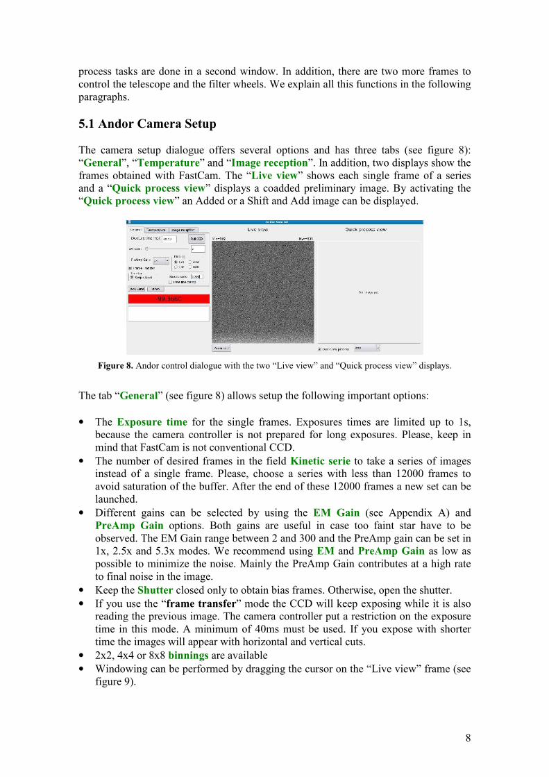
The camera setup dialogue offers several options and has three tabs (see figure 8):

“General”, “Temperature” and “Image reception”. In addition, two displays show the

frames obtained with FastCam. The “Live view” shows each single frame of a series

and a “Quick process view” displays a coadded preliminary image. By activating the

“Quick process view” an Added or a Shift and Add image can be displayed.

Figure 8. Andor control dialogue with the two “Live view” and “Quick process view” displays.

The tab “General” (see figure 8) allows setup the following important options:

• The Exposure time for the single frames. Exposures times are limited up to 1s,

because the camera controller is not prepared for long exposures. Please, keep in

mind that FastCam is not conventional CCD.

• The number of desired frames in the field Kinetic serie to take a series of images

instead of a single frame. Please, choose a series with less than 12000 frames to

avoid saturation of the buffer. After the end of these 12000 frames a new set can be

launched.

• Different gains can be selected by using the EM Gain (see Appendix A) and

PreAmp Gain options. Both gains are useful in case too faint star have to be

observed. The EM Gain range between 2 and 300 and the PreAmp gain can be set in

1x, 2.5x and 5.3x modes. We recommend using EM and PreAmp Gain as low as

possible to minimize the noise. Mainly the PreAmp Gain contributes at a high rate

to final noise in the image.

• Keep the Shutter closed only to obtain bias frames. Otherwise, open the shutter.

• If you use the “frame transfer” mode the CCD will keep exposing while it is also

reading the previous image. The camera controller put a restriction on the exposure

time in this mode. A minimum of 40ms must be used. If you expose with shorter

time the images will appear with horizontal and vertical cuts.

• 2x2, 4x4 or 8x8 binnings are available

• Windowing can be performed by dragging the cursor on the “Live view” frame (see

figure 9).

9

Figure 9. Windows can be selected by dragging the cursor on any point of the “Live view” display.

The window can be designed with any dimension and can be placed at any point within

the frame. Press “Full CCD” button to cancel the windowed mode. The “power of 2”

button applies this grey-scale option to enhance the contrast of the image.

Select the temperature of the CCD within the tab “Temperature” (see figure 10a) and

remember to press the “Cooler on” option to activate the cooling. A normal working

temperature is about -90 ºC. In the “Image reception” tab do not activate “Do not send

images” so that the frames can be displayed in the “Live view”.

After these steps, the camera should be ready to take images by pressing “Video”.

(a)

(b)

Figure 10. Temperature (a) and Image reception (b) tabs inside the Andor control dialogue.

5.2 Changing filters

The filter wheels are controlled through a custom application (see figure 11) in “alebo”

computer. FastCam has usually two wheels, one with standard broadband Johnson-

Bessell filters and a second wheel with narrow band filters. However, take into account

that the TCS dichroic sends the visible light to the autoguiding camera (FOVIA) while

only infrared bands (>700nm) arrive to FastCam so, by the moment, only red-infrared

bands can be used to observe with FastCam at the TCS. This will be solved in the next

future.

10

Figure 11. Filter wheel dialogue.

Because of the dichroic, and in case you do not need accurate photometry, we

recommend setting the Johnson filter wheel in a clear position. With this configuration I

and z bands will arrive to the FastCam detector with the maximum efficiency. Use I

filter if you want to reduce the atmospheric dispersion effects.

5.3 Bias and flat-fields

In the case of science cubes obtained in Lucky Imaging mode for astrometry purpose it

is not necessary to obtain dedicated bias or flat field cubes for each science target. In

fact, most pixels of your science cube will contain nothing else than blank sky, and

these are perfectly suited to determine bias level and bias structure from the science

data. In any case, the procedure to obtain bias frames is as follows: close the shutter

using “Shutter – Keep closed” in the Andor control dialogue, turn the lights off inside

the dome, close the mirror covers, and take a cube of images with the minimum

exposure time (typically 10 ms with the “frame transfer” mode off).

Flat-fields can be obtained using dome illumination. In order to obtain good signal

switch all the lights on and open the mirror covers. Then expose and process the series

using the “Add” option (lucky imaging has no sense for these frames). Figure 12 shows

a typical flat-field of FastCam.

Figure 12. Typical FastCam flat-field frame.

5.4 Telescope control from FastCam

FastCam is now able to connect with the telescope to point to the targets and to get

some data (airmass, ST, etc.) from the telescope control. This is done through the

“Telescope control” dialogue (see figure 13). There are two ways to add a target:

typing its coordinates by hand or loading a previously created catalogue from a browser

using the “Catalogues” option. Once the catalogue is loaded, the targets are selected by

clicking twice. Then press “Go” to point the telescope. The telescope can be stopped by

pressing “Stop” in any moment or parked to the zenith position by pressing “PARK”.

11

Default values can be restored by pressing “Reset”. Targets out of limits cannot by

pointed. In this case, the talker window will show a message in red advising the user of

this problem.

The “info” tab gives the actual position of the telescope. In this space the user can find

RA and Dec coordinates, Time and Airmass updated every two seconds.

Figure 13. “Telescope control” dialogue and “Info” tab

System catalogues, such as the SAO catalogue, are available. The user catalogues have

to be saved as text files “*.txt” in the /home/FastCam/cats directory following the

format:

Target1 21:12:34 +07:56:34 J 2000

Target2 15:11:12 +12:28:08 J 2000

Target3 05:23:34 +13:23:31 J 2000

Target4 12:06:54 +16:34:28 J 2000

… … … … …

6. Data saving and processing

FastCam uses custom software to acquire and save the data. This software can receive

the raw images from the Andor PC and saves as many series of images as the user

defines while the Andor CCD keeps exposing. This acquisition software starts by

launching the fastcam icon in the fastcam session desktop. This will open the window

shown in figure 14.

12

Figure 14. “Files” tab of the software to register and process the images.

The software has two display windows: one of them, left side, shows the images

registered, whilst the other, right side, shows a first result of a stacked and reduced

image. The software also shows the derived image, that enhances the contrast of the star

on the background sky. When the cursor is on these windows, 1D-profiles are shown.

(a)

(b)

Figure 15. (a) “Network” tab to acquire the images.

(b) “Config” tab to connect the Andor camera and to set the IPs and MACs.

The acquisition of images is performed from the tab “Network” (figure 15a). The left

part of this tab shows the header to be sent to the fits cubes. The right part of this tab is

dedicated to select the name of the file, storing directory, number of frames and series.

The cubes will be stored when pressing the “Process” button. If the “Processed” option

is active in the “Save” region, the software will process each cube separately. “Red +

Proc” option saves processed and reduced images, taking into account bias and flat-

field frames.

The software recognizes automatically the size of the image when a window is used (see

figure 9). On the left side, upper panel, the “Region” or “Track” options give different

ways to follow the speckle pattern in a set of frames and to stack them.

13

The raw frames saved are processed using the configuration set in the “Files” tab,

showed in figure 14. In a first place, the input files must be loaded enabling the “Load

and Process” option and selecting the processing parameters. The reduction can use the

bias images (we do not recommend to use flats; see section 5) selecting them in the

“Reductions” section.

One of the most important characteristics of this software is the method applied to stack

the images. There are three options (central panel):

1. “Add” stacks the 100% of the images producing a final image with the quality of a long exposure. The FWHM of the stars in this image is the natural seeing.

(see Section 9.1.1)

2. “Shift and add” computes offsets respect to the hottest pixel in each frame and stacks the 100% of the frames shifting them to a common reference point. This

reduction way does not select the best quality frames.

3. “Lucky images” selects the best quality images, compute the offsets and stacks the selected frames. The percentage of frames to be kept can be selected. This

process offers just the images with the best resolution which, if the number of

images to be kept is too low, can lead to a final image not too deep due to a low

effective exposure time. Usually, keeping a 20-30% of the images leads to

excellent results with good resolution and deepness. When observing a close

binary with components of similar magnitude click on the “Two stars” label.

This mode will avoid ghost stars in the processed image.

In some cases, the lucky imaging procedure yields black and flat frames or doubled

ghost targets in wrong positions. These effects are due to bad centered frames because

of the presence of cosmic rays or hot pixels. To correct this, we recommend the use of

the “Region” option marking the position of the target. The software will stack the

frames computing the position within this region.

Once established the reduction parameters the process is launched with the “Run”

button. The reduction process can be performed in iterative way, by using as inputs

other images previously reduced. The processed images can be saved using the

“output” parameters. The software allows the reduction of a maximum of 2 cubes of

1000 raw fits in a single shot.

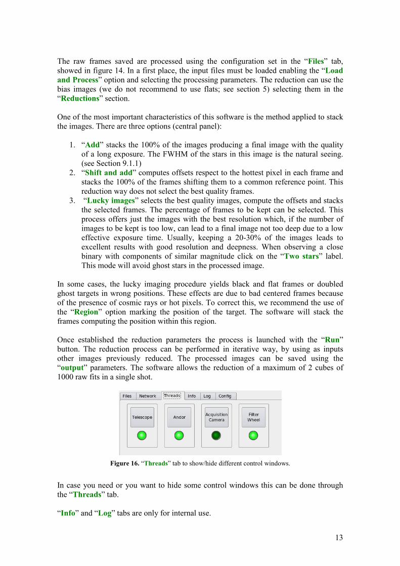
Figure 16. “Threads” tab to show/hide different control windows.

In case you need or you want to hide some control windows this can be done through

the “Threads” tab.

“Info” and “Log” tabs are only for internal use.

14

7. Exploring the reduced images

FastCam software also provides a function, “Inspector”, to explore the reduced images.

It is launched by clicking on the “inspect” button in the image registering software

(right side of figure 14), having the aspect showed in figure 17.

This environment is similar to the ds9 Saoimage tool, with user-friendly software. The

color map, palette and scales of the displays can be modified with the options appearing

at the upper right corner. The inspector displays both the direct image and the derived

image, although the contrast in the latter is higher and so objects such close binaries can

be distinguished much better here than in the direct image.

Inspector provides a rule to measure the distance between stars on the display. Firstly,

the pixel scale value has to be introduced (the usual pixel scale at the TCS is 42

mas/pix) and then, using the right button of the mouse and dragging on the display, the

user can estimate angular distances on the image. In addition, inspector provides

statistics of the image.

Figure 17. The inspector display.

15

8. Shutting down

1. Disable the cooling in the Temperature tab and close the water cycling pressing the “Start/Stop” button in the cooler device (see figure 7). Then, shutdown this

device.

2. Close the andor control software and disconnect telesforo from alebo. 3. Close the storage and processing software in alebo and exit from the “fastcam”

account.

4. Switch the instrument off and shutdown the “telesforo” computer (just behind the telescope M1).

9. Some recommendations

9.1 Finding the right gain exposure time

Golden rule: use the shortest possible exposure time in frame transfer mode. This will

offer a better temporal sampling of the speckle pattern. Of course, if the target is rather

dim and the maximum EM gain setting of 300 is already been used then the exposure

time must be increased. As a rule of thumb, to guarantee you are working in the linear

range of the detector, the maximum count value should be around 4,000 ADU, when the

EM gain is high.

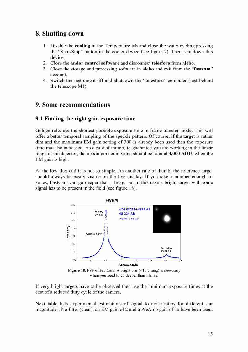
At the low flux end it is not so simple. As another rule of thumb, the reference target

should always be easily visible on the live display. If you take a number enough of

series, FastCam can go deeper than 11mag, but in this case a bright target with some

signal has to be present in the field (see figure 18).

Figure 18. PSF of FastCam. A bright star (<10.5 mag) is necessary

when you need to go deeper than 11mag.

If very bright targets have to be observed then use the minimum exposure times at the

cost of a reduced duty cycle of the camera.

Next table lists experimental estimations of signal to noise ratios for different star

magnitudes. No filter (clear), an EM gain of 2 and a PreAmp gain of 1x have been used.

16

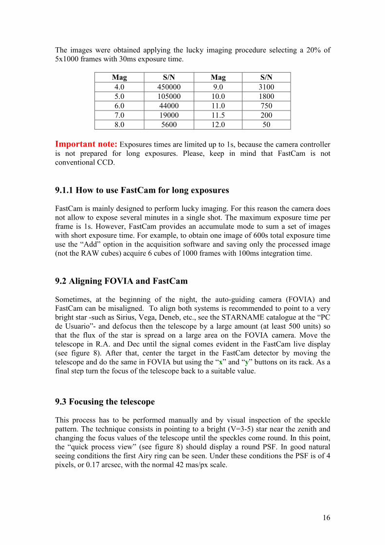
The images were obtained applying the lucky imaging procedure selecting a 20% of

5x1000 frames with 30ms exposure time.

Mag S/N Mag S/N

4.0 450000 9.0 3100

5.0 105000 10.0 1800

6.0 44000 11.0 750

7.0 19000 11.5 200

8.0 5600 12.0 50

Important note: Exposures times are limited up to 1s, because the camera controller is not prepared for long exposures. Please, keep in mind that FastCam is not

conventional CCD.

9.1.1 How to use FastCam for long exposures

FastCam is mainly designed to perform lucky imaging. For this reason the camera does

not allow to expose several minutes in a single shot. The maximum exposure time per

frame is 1s. However, FastCam provides an accumulate mode to sum a set of images

with short exposure time. For example, to obtain one image of 600s total exposure time

use the “Add” option in the acquisition software and saving only the processed image

(not the RAW cubes) acquire 6 cubes of 1000 frames with 100ms integration time.

9.2 Aligning FOVIA and FastCam

Sometimes, at the beginning of the night, the auto-guiding camera (FOVIA) and

FastCam can be misaligned. To align both systems is recommended to point to a very

bright star -such as Sirius, Vega, Deneb, etc., see the STARNAME catalogue at the “PC

de Usuario”- and defocus then the telescope by a large amount (at least 500 units) so

that the flux of the star is spread on a large area on the FOVIA camera. Move the

telescope in R.A. and Dec until the signal comes evident in the FastCam live display

(see figure 8). After that, center the target in the FastCam detector by moving the

telescope and do the same in FOVIA but using the “x” and “y” buttons on its rack. As a

final step turn the focus of the telescope back to a suitable value.

9.3 Focusing the telescope

This process has to be performed manually and by visual inspection of the speckle

pattern. The technique consists in pointing to a bright (V=3-5) star near the zenith and

changing the focus values of the telescope until the speckles come round. In this point,

the “quick process view” (see figure 8) should display a round PSF. In good natural

seeing conditions the first Airy ring can be seen. Under these conditions the PSF is of 4

pixels, or 0.17 arcsec, with the normal 42 mas/px scale.

17

9.4 Pixel Scale and field orientation

The pixel scale of FastCam in the TCS is of ∼42mas/px. The orientation is North to the

left and East down, but this reference system is turned about 1.5 deg from North to East.

We recommend the observer to acquire calibrations in the core of globular clusters with

HST astrometry or binaries with well known separation to calibrate the pixel scale and

the orientation each night (or at least each observing run). Double stars for calibrations

can be retrieved from the Washington Double Star Sixth catalogue, available in

http://ad.usno.navy.mil/wds/

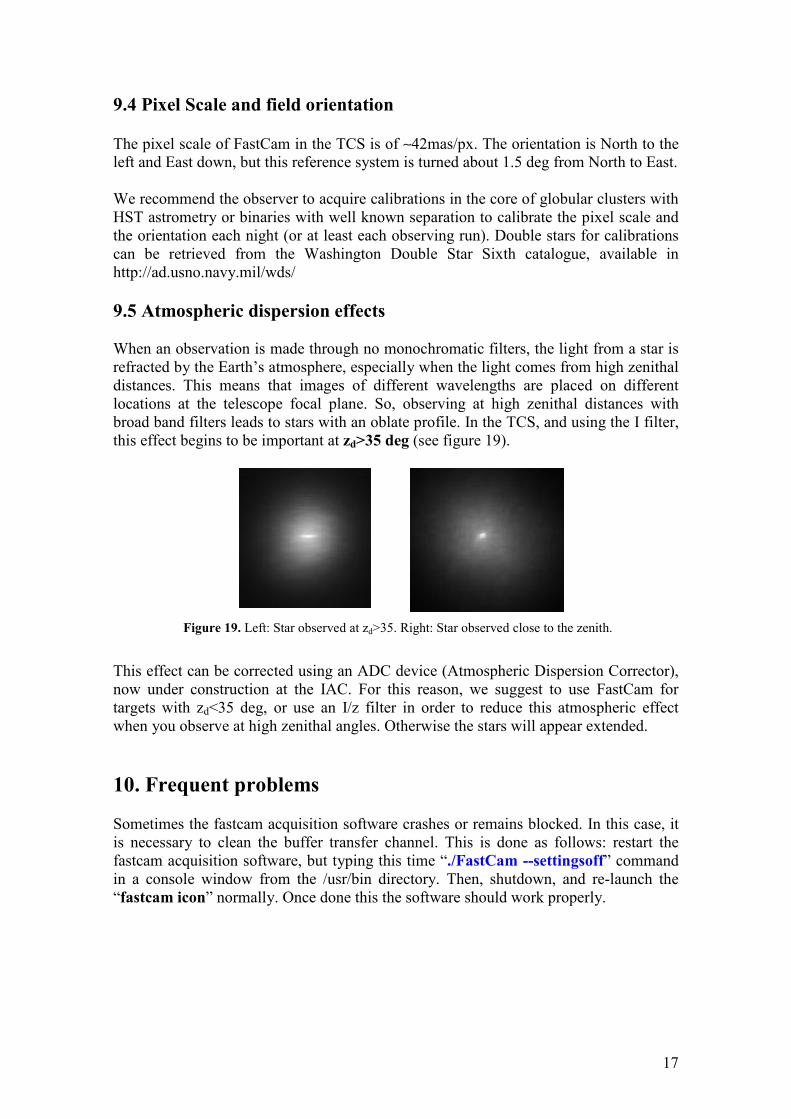
9.5 Atmospheric dispersion effects

When an observation is made through no monochromatic filters, the light from a star is

refracted by the Earth’s atmosphere, especially when the light comes from high zenithal

distances. This means that images of different wavelengths are placed on different

locations at the telescope focal plane. So, observing at high zenithal distances with

broad band filters leads to stars with an oblate profile. In the TCS, and using the I filter,

this effect begins to be important at zd>35 deg (see figure 19).

Figure 19. Left: Star observed at zd>35. Right: Star observed close to the zenith.

This effect can be corrected using an ADC device (Atmospheric Dispersion Corrector),

now under construction at the IAC. For this reason, we suggest to use FastCam for

targets with zd<35 deg, or use an I/z filter in order to reduce this atmospheric effect

when you observe at high zenithal angles. Otherwise the stars will appear extended.

10. Frequent problems

Sometimes the fastcam acquisition software crashes or remains blocked. In this case, it

is necessary to clean the buffer transfer channel. This is done as follows: restart the

fastcam acquisition software, but typing this time “./FastCam --settingsoff” command

in a console window from the /usr/bin directory. Then, shutdown, and re-launch the

“fastcam icon” normally. Once done this the software should work properly.

18

11. References [1] J. M. Beckers, “Adaptive optics for astronomy: Principles, performance and

applications,” in Annual review of astronomy and astrophysics, vol. 31.(1993). [2] Dantowitz, D., “Shaper Images Through Video”, in Sky & Telescope, August 1998. [3] D. L. Fried, “The nature of atmospheric turbulence effects on imaging and pseudo-

imaging systems, and its quantification”, University of Sydney, 1979, p. 4-1 to 4-43. [4] F. Gago, L. Rodriguez-Ramos, G. Herrera, J. Gigante A. Alonso, T. Viera, J.

Piqueras, and J. Diaz, “Tip-tilt mirror control based on FPGA for an adaptive optics

system,” in 3rd Southern Conference on Programmable Logic, 2007. SPL ’07. [5] N. M. Law, C. D. Mackay, and J. E. Baldwin, “Lucky imaging: high angular

resolution imaging in the visible from the ground,” in Astronomy and Astrophysics,

vol. 446, Feb, 2006, pp. 739–745 [6] A. Oscoz et al., “FastCam: a new lucky imaging instrument for medium-sized

telescopes”, Marseille, SPIE (2008). [7] L.F. Rodríguez-Ramos et al., “Real-time lucky imaging in FastCam project”,

Marseille, SPIE (2008). [8] L. F. Rodriguez-Ramos, T. Viera, G. Herrera, J. V. Gigante, F. Gago, and A.

Alonso, “Testing FPGAs for real-time control of of adaptive optics in giant

telescopes,” in Proceedings of SPIE - The International Society for Optical

Engineering, vol. 6272 July 2006. [9] L. F. Rodriguez-Ramos, A. Alonso, F. Gago, J. V. Gigante, G. Herrera, and T.

Viera, “Adaptive optics real-time control using FPGA,” in International Conference

on Field Programmable Logic and Applications 2006. FPL ’06. [10] Scardia, M. et al., “Speckle observations with PISCO in Merate - II. Astrometric

measurements of visual binaries in 2004”, MNRAS, 367, 1170 (2006). [11] Scardia, M. et al., “Speckle observations with PISCO in Merate - III. Astrometric

measurements of visual binaries in 2005 and scale calibration with a grating mask”,

MNRAS, 374, 965 (2007). [12] Tubbs, R. N., [PhD Thesis], Cambridge University (2003). [13] N. Labadie et al. “High contrast optical imaging of companions: the case of the

brown dwarf binary HD-130948BC”. Accepted for publication in A&A,

(http://xxx.unizar.es/abs/1009.5670).

19

Appendix A. On the EM gain

A note of caution. The gain components in an ICCD, an EMCCD and the EM register suffer from gain aging effects. For a given applied voltage to the gain

components you would expect the gain to remain constant. However the gain

components suffer from parasitic effects which lower their gain as a function of the

total charge extracted from them. Therefore if you measure the gain over a period of

time at a fixed voltage and temperature the gain will fall off and the fall off will be

more pronounced the more extracted charge that passes though the gain component.

The gain is not lost however and a certain gain can be recovered by simply

increasing the voltage in the gain component to compensate for the aging effect.

Ultimately the gain components can be damaged by excessive voltage so they do

have an ultimate lifetime.

To minimize the effects of gain aging it is desirable not to have the gain turned up

when the device is not recording signal and to use the gain sparingly i.e. set the gain

to give you sufficient sensitivity and not to use the gain at the maximum level

needlessly.

Appendix B. On the detector linearity

A linearity study has been done. Given the particular features of the EMCCD

detectors, the linearity changes depending on their PreAmp and EM gains. We

analyzed the detector response on October 2010 for several PreAmp and EM gains.

Figures 20 show the residuals from a linear fit for the whole dynamical range of the

detector. The following table lists the linearity limit for several gains.

20

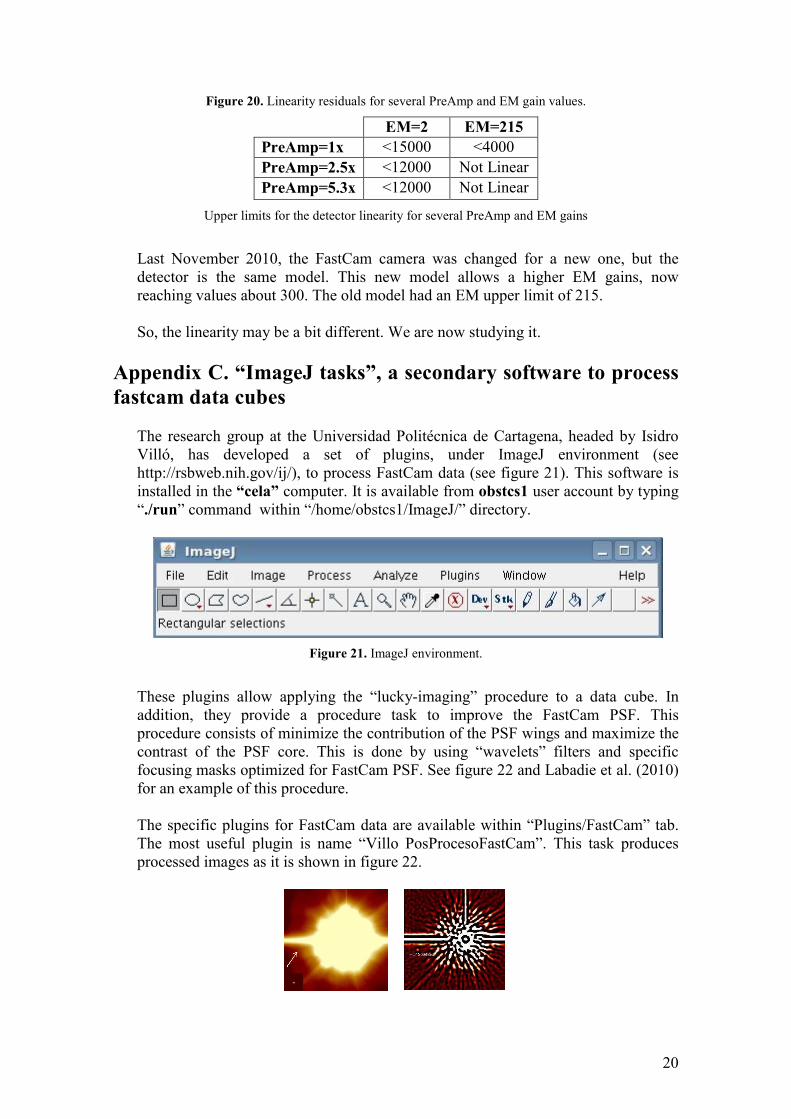
Figure 20. Linearity residuals for several PreAmp and EM gain values.

EM=2 EM=215

PreAmp=1x <15000 <4000

PreAmp=2.5x <12000 Not Linear

PreAmp=5.3x <12000 Not Linear

Upper limits for the detector linearity for several PreAmp and EM gains

Last November 2010, the FastCam camera was changed for a new one, but the

detector is the same model. This new model allows a higher EM gains, now

reaching values about 300. The old model had an EM upper limit of 215.

So, the linearity may be a bit different. We are now studying it.

Appendix C. “ImageJ tasks”, a secondary software to process

fastcam data cubes

The research group at the Universidad Politécnica de Cartagena, headed by Isidro

Villó, has developed a set of plugins, under ImageJ environment (see

http://rsbweb.nih.gov/ij/), to process FastCam data (see figure 21). This software is

installed in the “cela” computer. It is available from obstcs1 user account by typing

“./run” command within “/home/obstcs1/ImageJ/” directory.

Figure 21. ImageJ environment.

These plugins allow applying the “lucky-imaging” procedure to a data cube. In

addition, they provide a procedure task to improve the FastCam PSF. This

procedure consists of minimize the contribution of the PSF wings and maximize the

contrast of the PSF core. This is done by using “wavelets” filters and specific

focusing masks optimized for FastCam PSF. See figure 22 and Labadie et al. (2010)

for an example of this procedure.

The specific plugins for FastCam data are available within “Plugins/FastCam” tab.

The most useful plugin is name “Villo PosProcesoFastCam”. This task produces

processed images as it is shown in figure 22.

21

Figure 22. Left panel: Stacked image using lucky-image procedure of

HD130948. Right panel: Post-processed image using wavelets and focusing

masks (from Labadie et al. 2010).