Fast Space-varying Convolution and Its Application in ... · Fast Space-varying Convolution and Its...

Fast Space-varying Convolution and Its Application in StrayLight Reduction*

Jianing Weia, Guangzhi Caoa, Charles A. Boumana, and Jan P. Allebacha

aSchool of Electrical Engineering, Purdue University, West Lafayette, IN 47907-0501, USA

ABSTRACT

Space-varying convolution often arises in the modeling or restoration of images captured by optical imagingsystems. For example, in applications such as microscopy or photography the distortions introduced by lensestypically vary across the field of view, so accurate restoration also requires the use of space-varying convolu-tion. While space-invariant convolution can be efficiently implemented with the Fast Fourier Transform (FFT),space-varying convolution requires direct implementation of the convolution operation, which can be very com-putationally expensive when the convolution kernel is large.

In this paper, we develop a general approach to the efficient implementation of space-varying convolutionthrough the use of matrix source coding techniques. This method can dramatically reduce computation byapproximately factoring the dense space-varying convolution operator into a product of sparse transforms. Thisapproach leads to a tradeoff between the accuracy and speed of the operation that is closely related to thedistortion-rate tradeoff that is commonly made in lossy source coding.

We apply our method to the problem of stray light reduction for digital photographs, where convolutionwith a spatially varying stray light point spread function is required. The experimental results show that ouralgorithm can achieve a dramatic reduction in computation while achieving high accuracy.

Keywords: space-varying convolution, stray light, image restoration, matrix source coding

1. INTRODUCTION

Space-varying convolution often arises in the modeling or restoration of images captured by optical imagingsystems. This is due to the fact that the point spread function (PSF) and/or distortion introduced by a lenstypically varies across the field of view,1 so accurate restoration also requires the use of space-varying convolution.

In this work, we will consider the problem of stray light reduction for digital photographs.2 In all opticalimaging systems, a small portion of the entering light flux is misdirected to undesired locations in the imageplane. We refer to this severely misdirected light as stray light, but it is sometimes referred to as lens flare orveiling glare.1 Causes for this phenomena include but are not limited to: (1) Fresnel reflections from opticalelement surfaces; (2) scattering from surface imperfections on lens elements; (3) scattering from air bubbles intransparent glass or plastic lens elements; and (4) scattering from dust or other particles.

The stray light reduction algorithm is originally due to Jansson and Fralinger.3 It can be described by2, 4 thefollowing equation:

x = 2y − (1 − β)y − βSy, (1)

where y is the observed image, x is the estimate of the underlying image to be recovered, S is a matrix representingconvolution with the stray light PSF, and β is the weight of stray light. If S implements space-invariant 2Dcircular convolution, then Sy can be computed using a 2D FFT, which can dramatically reduce computation.5

*Research partially supported by E. I. du Pont De Nemours and Company.Further author information: (Send correspondence to Jianing Wei)Jianing Wei: E-mail: [email protected], Telephone: 1 765 494 3465Guangzhi Cao: E-mail: [email protected], Telephone: 1 765 494 6553Charles A. Bouman: E-mail: [email protected], Telephone: 1 765 494 0340Jan P. Allebach: E-mail: [email protected], Telephone: 1 765 494 3535

Computational Imaging VII, edited by Charles A. Bouman, Eric L. Miller, Ilya Pollak, Proc. of SPIE-IS&T Electronic Imaging,SPIE Vol. 7246, 72460B · © 2009 SPIE-IS&T · CCC code: 0277-786X/09/$18 · doi: 10.1117/12.813512

SPIE-IS&T/ Vol. 7246 72460B-1

Downloaded from SPIE Digital Library on 12 Jan 2010 to 128.46.156.233. Terms of Use: http://spiedl.org/terms

However, the stray light PSF is space-varying, so FFT cannot be directly used to speed up computation. Inaddition, the support of the stray light PSF is very large, which makes S a dense matrix, and the computationof Sy extremely expensive. If the image contains N pixels, the computation is O(N2). For a 106 pixel image, ittakes 106 multiplies to compute each output pixel, resulting in a total of 1012 multiplies. This means hours ofprocessing time, which makes it infeasible for real-world applications of the stray light reduction algorithm.

In this paper, we introduce a novel approach for efficient computation of space-varying convolution, based onthe theory of matrix source coding;6 and we demonstrate how the technique can be used to efficiently implementthe stray light reduction for digital cameras. The matrix source coding technique uses the method of lossy sourcecoding which makes the dense matrix S sparse. This is done by first decorrelating the rows and columns of S andthen quantizing the resulting compacted matrix so that most of its entries become zero. By making S sparse, wenot only save storage, but we also dramatically reduce the computation of the required matrix-vector product.

Our experimental results indicate that, by using this approach, we can reduce the computational complexityof space-varying convolution from O(N2) to O(N). For digital images exceeding 1 Meg pixel in size, this makesdeconvolution practically possible, and results in deconvolution algorithms that can be computed with 5 to 10multiplies per output pixel.

In the rest of this paper, we start by introducing the stray light contamination model and the algorithm forstray light reduction. We then elaborate on the theory and implementation of the matrix source coding approachfor space-varying convolution with the stray light point spread function. Finally, we present experimental resultsto demonstrate the effectiveness of our algorithm.

2. STRAY LIGHT REDUCTION STRATEGY

2.1 PSF Model FormulationThe PSF model for a stray light contaminated optical imaging system is supposed to account for the followingcontributions: (1) diffractive spreading owing to the finite aperture of the imaging device; (2) aberrations arisingfrom non-ideal aspects of the device design and device fabrication material; and (3) stray light due to scatteringand undesired reflections. Therefore, the forward model of stray light contamination can be expressed as

y = ((1 − β)G + βS)x, (2)

where G accounts for diffraction and aberration, S accounts for stray light due to scattering and undesiredreflections, β represents the weight factor of stray light. The entries of G are described by

Gq,p = g(iq, jq; ip, jp),

where (ip, jp) and (iq, jq) are the 2D positions of the input and output pixel locations, measured relative to thecenter of the camera’s field of view. Using this notation, we have modeled the diffraction and aberration PSFwith the following function2, 4, 7, 8

g(iq, jq; ip, jp) =1

2πσ2exp

(− (iq − ip)2 + (jq − jp)2

2σ2

). (3)

Similarly, the entries of S are described by

Sq,p = s(iq, jq; ip, jp).

We model this stray light PSF with the following function2, 4, 7, 8

s(iq, jq; ip, jp) =1z

1(1 + 1

i2p+j2p

((iqip+jqjp−i2p−j2

p)2

(c+a(i2p+j2p))2 + (−iqjp+jqip)2

(c+b(i2p+j2p))2

))α , (4)

where z is a normalizing constant that makes∫

iq

∫jq

s(iq, jq; ip, jp)diqdjq = 1. An analytic expression for z isz = π

α−1 (c + a(i2p + j2p))(c + b(i2p + j2

p)). The model parameters are then (a, b, c, α, β, σ). Previous work2, 4, 7, 8

has established an approach for estimating these parameters. We use the same apparatus and algorithm to doparameter estimation.

SPIE-IS&T/ Vol. 7246 72460B-2


2.2 Stray Light Reduction

Once the model parameters are estimated, we use Van Cittert’s method9, 10 to compute the restored image. VanCittert’s method is an iterative approach to restore images. The iteration formula is as follows:

x(k+1) = x(k) + y − Ax(k), (5)

where x(k) is the estimate of the original image at the kth iteration, A = ((1 − β)G + βS), and we initializex(0) with the observed image y. We can approximate the diffraction and aberration PSF with a delta function,2

leading to G = I. It has been shown that the result of the first iteration is already a good estimate of the originalimage.2 Therefore, our restoration equation becomes:

x = 2y − (1 − β)y − βSy. (6)

However, since our stray light PSF is global and space-varying, directly computing Sy is quite expensive. For a6 Megapixel image, it requires 6 million multiplies per output pixel, and a total of 3.6 × 1013 multiplies. So wecompress the transform matrix S using matrix source coding to reduce the on-line computation.

3. MATRIX SOURCE CODING

3.1 Matrix Source Coding Theory

The computationally expensive part in Eq. (6) is

x = Sy. (7)

Our strategy for speeding up computation is to compress the matrix S, such that it becomes sparse. In order tofind a sparse representation of the matrix S, we use the techniques of lossy source coding. Let [S] represent thequantized version of S. Then S = [S] + δS, where δS is the quantization error. This error δS results in somedistortion in x given by

δx = δSy. (8)

A conventional distortion metric for the source coding of the matrix S is ‖δS‖2. However, this may be verydifferent from the squared error distortion in the matrix-vector product result which is given by ‖δx‖2. Therefore,we would like to relate the distortion metric for S to the quantity ‖δx‖2.

It has been shown that if the image y and the quantization error δS are independent, then the distortion inx is given by6, 11

E[‖δx‖2|δS]

= ‖δS‖2Ry

= trace{δSRyδSt}, (9)

where Ry = E[yyt]. So if the data vector y is white, then Ry = I, and

E[‖δx‖2|δS]

= ‖δS‖2. (10)

In other words, when the data is white, minimizing the squared error distortion of the matrix S is equivalent tominimizing the expected value of the squared error distortion for the restored image x.

So our strategy for source coding of matrix S is to simultaneously:

• Whiten the image y, so that minimizing the distortion in the coded matrix is equivalent to minimizing thedistortion in the restored image.

• Decorrelate the columns of S, so that they will code more efficiently after quantization.

• Decorrelate the rows of S, so that they will code more efficiently after quantization.

SPIE-IS&T/ Vol. 7246 72460B-3


The above goals can be achieved by applying the following transformation

S = W1ST−1 (11)y = Ty, (12)

where T is a matrix that simultaneously whitens the components of y and decorrelates the columns of S, and W1

is a matrix that approximately decorrelates the rows of S. In our case, W1 is a wavelet transform, since wavelettransforms are known to be an approximation to the Karhunen-Loeve transform for stationary sources, and arecommonly used as decorrelating transforms.12 We form the matrix T by applying a wavelet transform to y

followed by gain factors designed to normalize the variance of the wavelet coefficients. Specifically, T = Λ−1/2w W2

and T−1 = W−12 Λ1/2

w , where W2 is also a wavelet transform, and Λ−1/2w is a diagonal matrix of gain factors

designed so thatΛw = E[diag(W2yytW t

2)].

This matrix T approximately whitens and decorrelates the image y. The diagonal matrix Λw can be estimatedfrom training images. We take the wavelet transform W2 of these training images, compute the variance ofwavelet coefficients in each band, and average over all images. In this way, we only have a single gain factor foreach band of the wavelet transform.

Using the above matrix source coding technique, the computation of the space-varying convolution nowbecomes

x ≈ W−11 [S]y, (13)

where [S] is the quantized version of S. Therefore, the on-line computation consists of two wavelet transformsand a sparse matrix vector multiply. We will show later that this technique results in huge savings in computationof space-varying convolution.

3.2 Efficient Implementation of Matrix Source Coding

In order to implement the fast space-varying convolution method of Eq. (13), it is first necessary to computethe source coded matrix [S]. We will refer to the computation of [S] as the off-line portion of the computation.Once the sparse matrix [S] is available, then the space-varying convolution may be efficiently computed usingon-line computation shown in Eq. (13).

However, even though the computation of [S] is performed off-line, rigorous evaluation of this sparse matrixis still too large for practical problems. For example, if the image is 16 Megapixel in size, then temporary storageof S requires approximately 1 Petabyte of memory. The following section describes an efficient approach tocompute [S] which eliminates the need for any such temporary storage.

In our implementation, we use the Haar wavelet transform13 for both W2 and W1. The Haar wavelet transformis an orthonormal transform, so we have that

S = W1ST−1

= W1SW t2Λ1/2

w .

Therefore, the precomputation consists of a wavelet transform W2 along the rows of S, scaling of the matrixentries, and a wavelet transform W1 along the columns. Unfortunately, the computational complexity of thesetwo operations is O(N2), where N is the number of pixels in the image, because the operation requires that eachentry of S be touched. In order to reduce this computation to order O(N), we will use a two stage quantizationprocedure combined with a recursive top-down algorithm for computing the Haar wavelet transform coefficients.

The first stage of this procedure is to reduce the computation of the wavelet transform W1. To do this, wefirst compute the wavelet transform of each row using W2, and then we perform an initial quantization step.This procedure is expressed mathematically as

[S] ≈ [W1[SW t2Λ1/2

w ]], (14)

SPIE-IS&T/ Vol. 7246 72460B-4


where the notation [· · · ] denotes quantization. After the initial quantization, the resulting matrix [SW t2Λ1/2

w ] isquite sparse. If the number of remaining nonzero entries in each row is K, then the computational complexityof the second wavelet transform W1 is reduced to order O(KN) rather than O(N2).

However, the problem still remains as to how to efficiently implement the first wavelet transform W2, sincenaive application of W2 to every row still requires O(N2) operations. The next section describes an approach forefficiently computing this first wavelet transform by only evaluating the significant coefficients. This can be doneby using a top-down recursive method to only evaluate the wavelet coefficients that are likely to have absolutevalues substantially larger than zero.

3.2.1 Determining the Location of Significant Wavelet Coefficients

As discussed above, we need a method for computing only the significant wavelet coefficients in order to reducethe complexity of the wavelet transform W2. To do this, we will first predict the location of the largest K entriesin every row of the matrix SW t

2Λ1/2w . Then we will present an approach for computing only those coefficients,

without the need to compute all coefficients in the transform.

Since each row of S is actually an image, we will use the 2D index (iq, jq) to index a row S, and (ip, jp)to index a column of S. Using this notation, S(iq,jq),(ip,jp) represents the effect of the point source at position(ip, jp) on the output pixel location (iq, jq).

Figure 1(a) shows an example of the row of S displayed as an image, together with its wavelet transform inFig. 1(b). The wavelet transform is then scaled by gain factors Λ−1/2

w , and represented by the corresponding rowof SW t

2Λ1/2w . Finally, Fig. 1(c) shows the locations of the wavelet coefficients that are non-zero after quantization,

and a circle in each band that is used to indicate the region containing all non-zero entries.

By identifying the regions containing non-zero wavelet coefficients, we can reduce computation. In practice,we determine these regions by randomly selecting rows of the matrix and determining the center and maximumradius necessary to capture all non-zero coefficients.

3.2.2 A Top-Down Approach for Computing Sparse Haar Wavelet Coefficients

In order to efficiently compute sparse Haar wavelet coefficients, we compute only the necessary approximationcoefficients at each level using a top-down tree-based approach. The tree structure is illustrated in Fig. 2. Sincethe approximation coefficients at different scales form a quad-tree, the value of each node can be computed fromits children as

fa[k][m][n] =12(fa[k − 1][2m][2n] + fa[k − 1][2m + 1][2n]

+fa[k − 1][2m][2n + 1] + fa[k − 1][2m + 1][2n + 1]), (15)

where fa[k][m][n] represents an approximation coefficient at level k and location (m, n). Here level k = 0 isthe lowest level corresponding to the full resolution image. A recursive algorithm can be easily formulated fromEq. (15). We know that when the corresponding detail coefficients of an approximation coefficient are all zero,it means that the approximation is perfect. So in this case, for the nodes whose corresponding detail coefficientsare all zeroed out after quantization, we stop and compute the value of the approximation coefficient by

fa[k][m][n] = 2kfa[0][2km][2kn]. (16)

Note that fa[0][2km][2kn] can be directly computed from the expression of the PSF. Another stopping pointoccurs when the leaves of the tree are reached, i.e. k = 0. Therefore, we have a recursive algorithm forcomputing the significant Haar wavelet approximation coefficients as shown in Fig. 3.

SPIE-IS&T/ Vol. 7246 72460B-5


1

100

100

000

400

500

000

700

000

000

1000

000 400 000 000 1000(1qJq

Z'AãW

I

iW

k+ 1

k

k-i

100 200 300 400 500 600 700 800 900 1000

100

200

300

400

500

600

700

800

900

1000

(a) An example of the row image. (b) The corresponding wavelet transform.

(c) Location of non-zero wavelet coefficients after quantization.

Figure 1. An example of a row of S displayed as an image together with its wavelet transform, and the locations ofnon-zero entries after quantization: (a) shows the log amplitude map of the row image, (b) shows the log of the absolute

value of its wavelet transform, (c) shows the locations of non-zero entries of the corresponding row of SW t2Λ

1/2w .

Figure 2. An illustration of the tree structure of approximation coefficients. Shaded squares indicate that the detailcoefficients are not zero at those locations. So we go to the next level recursion. Empty squares indicate that the detailcoefficients are zero, and we stop to compute their values.

After obtaining the significant approximation coefficients, we can compute the necessary wavelet coefficients13

using the following equation:

fhd [k][m][n] =

12(fa[k − 1][2m][2n]− fa[k − 1][2m][2n + 1] + fa[k − 1][2m + 1][2n] − fa[k − 1][2m + 1][2n + 1])

fvd [k][m][n] =

12(fa[k − 1][2m][2n] + fa[k − 1][2m][2n + 1] − fa[k − 1][2m + 1][2n] − fa[k − 1][2m + 1][2n + 1])

fdd [k][m][n] =

12(fa[k − 1][2m][2n]− fa[k − 1][2m][2n + 1] − fa[k − 1][2m + 1][2n] + fa[k − 1][2m + 1][2n + 1]),

(17)

where fhd [k][m][n], fv

d [k][m][n], and fdd [k][m][n] denote the horizontal, vertical, and diagonal detail coefficients

respectively, at level k, location (m, n). We can show that the complexity of our algorithm for computing

SPIE-IS&T/ Vol. 7246 72460B-6


float FastApproxCoef(k, m, n) {float value = 0;if (k==0) {

value = s(iq, jq ; m, n);fa[k][m][n] = value;return value;

}if (ZeroDetailCoef(k,m,n)) {

value = 2ks(iq, jq; 2km, 2kn);

fa[k][m][n] = value;return value;

}value += FastApproxCoef(k-1, 2m, 2n);value += FastApproxCoef(k-1, 2m, 2n+1);value += FastApproxCoef(k-1, 2m+1, 2n);value += FastApproxCoef(k-1, 2m+1, 2n+1);value = value/2;fa[k][m][n] = value;return value;

}(a) Primary function.

int ZeroDetailCoef(k,m,n) {if (d

`(m,n), (mk

c , nkc )

´> max{r(k)

h , r(k)v , r

(k)d }) {

/* (mkc , nk

c ) is the center of the circle at level k *//* d

`(m,n), (mk

c , nkc )

´is the distance from (m,n) to (mk

c , nkc ) */

return 1;}else {

return 0;}

}(b) Subroutine.

Figure 3. Pseudo code for fast computation of significant Haar approximation coefficients. Part (a) is the main routine.Part (b) is a subroutine called by (a). The approximation coefficient at level k, location (m, n) is denoted fa[k][m][n].

sparse Haar wavelet coefficients of an N -pixel image is O(K), where K represents the number of nonzero entriesafter quantization. The number of nodes that we visit in the tree of approximation coefficients is at most 4K.Computing these 4K nodes requires at most 16K additions. So the complexity of computing the approximationtree is O(K). Once the necessary approximation coefficients are computed, computing the detail coefficientsonly requires O(K) operations. Thus the complexity of our algorithm is O(K) for one row of S. Therefore, wereduce the complexity of precomputation of [S] from O(N2) to O(KN).

4. EXPERIMENTAL RESULTS

4.1 Experiments on Space-varying Convolution with Stray Light PSF

In order to test the performance of our algorithm in computing x = Sy, we use the test image shown inFig. 4 for y, and a realistic stray light PSF for S. The parameters of this PSF are: a = −1.65 × 10−5 mm−1,b = −5.35 × 10−5 mm−1, α = 1.31, c = 1.76 × 10−3 mm. The parameters of this PSF were estimated for anOlympus SP-510 UZ∗ camera. We picked three natural images as training images to obtain the scaling matrix

∗Olympus America Inc., Center Valley, PA 18034

SPIE-IS&T/ Vol. 7246 72460B-7


Figure 4. Test image for space-varying convolution with stray light PSF.

Λw. We use normalized root mean square error (NRMSE) as the distortion metric:

NRMSE =

√‖x − W−1

1 [S]y‖22

‖x‖22

. (18)

Our measure of computation is the average number of multiplies per output pixel (rate), which is given by theaverage number of non-zero entries in the sparse matrix [S] divided by the total number of pixels N .

In order to better understand the computational savings, we used two different image sizes of 256× 256 and1024 × 1024 for our experiments. In the 256× 256 case, we used an eight level Haar wavelet transform for W2.In the 1024× 1024 case, we used a ten level Haar wavelet transform for W2. In both cases, W1 was chosen to bea three level CDF 5-3 wavelet transform.14 In addition, the wavelet transform W1 was computed using a 64× 64block structure so as to minimize the size of temporary storage used in the off-line computation. Using a blockstructure enables us to compute the rows of [SW t

2Λ1/2w ] corresponding to one block, take the wavelet transform

along the columns, then quantize and save, and then go to the next block.

Figure 5(a) shows the distortion rate curves for a 256× 256 image using two different techniques, i.e. simplequantization of S and matrix source coding of S as described by Eq. (13). Note that direct multiplication by Swithout quantization requires 65, 536 multiplies per output pixel.

Figure 5(b) compares the distortion rate curves of our matrix source coding algorithm on two different imagesizes — 256 × 256 and 1024 × 1024. Notice that the computation per output pixel actually decreases with theimage resolution. This is interesting since the computation of direct multiplication by S increases linearly withthe size of the image N .

At 1024× 1024 resolution, with only 2% distortion, our algorithm reduces the computation from 1048576 =10242 multiplies per output pixel to 12 multiplies per output pixel; and that is a 87, 381:1 reduction in compu-tation.

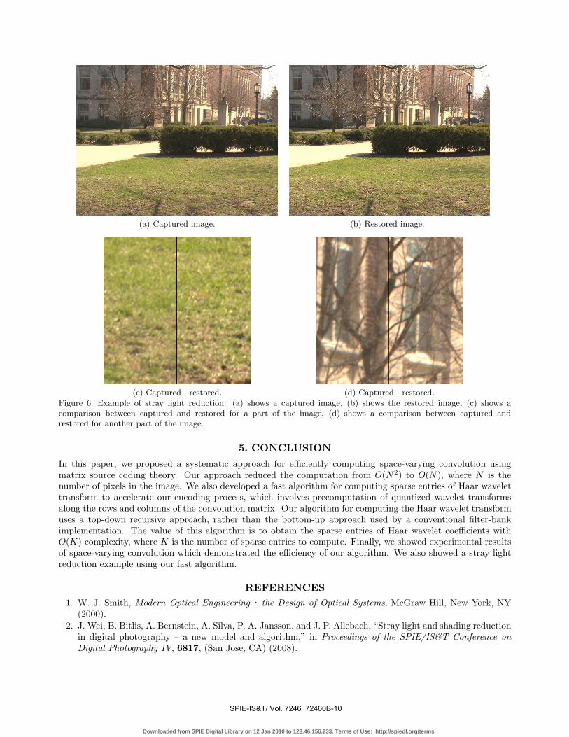
4.2 Experiment on Stray Light ReductionWe use Eq. (6) to perform stray light reduction. The space-varying convolution Sy is efficiently computed usingour matrix source coding approach. We take outdoor images with an Olympus SP-510UZ camera. The straylight PSF parameters were shown in the previous subsection. The other parameter β = 0.3937. We use an eightlevel Haar wavelet for W2, and a three level CDF 5-3 wavelet14 for W1, with block structure of block size 64×64.

Figure 4.2 shows an example of stray light reduction. Figure 4.2(a) is the captured image. Figure 4.2(b) isthe restored image. Figures 4.2(c-d) shows a comparison between captured and restored versions for differentparts of the image. From this example, we can see that the stray light reduction algorithm increases the contrastand recovers more details of the original scene.

SPIE-IS&T/ Vol. 7246 72460B-8


0 10 20 30 40 50 60 700

0.1

0.2

0.3

0.4

0.5

0.6

0.7

0.8

0.9

1

multiplies per output

NR

MS

E

matrix source coding of Sdirect quantization of S

(a) Distortion vs. computation for two methods on image size 256 × 256.

0 5 10 15 20 25 30 35 400

0.02

0.04

0.06

0.08

0.1

0.12

multiplies per output

NR

MS

E

image size 256x256image size 1024x1024

(b) Distortion vs. computation for two image sizes using matrix source coding of S.

Figure 5. Experiments demonstrating fast space-varying convolution with stray light PSF: (a) relative distortion versusnumber of multiplies per output pixel (i.e. rate) using two different matrix source coding strategies: the black solid lineshows the curve for our proposed matrix source coding algorithm as described in Eq. (13), and the red dashed line showsthe curve resulting from direct quantization of the matrix S; (b) comparison of relative distortion versus computationbetween two different resolutions: the solid black line shows the curve for 256 × 256, and the dashed blue line shows thecurve for 1024 × 1024.

SPIE-IS&T/ Vol. 7246 72460B-9


(a) Captured image. (b) Restored image.

(c) Captured | restored. (d) Captured | restored.

Figure 6. Example of stray light reduction: (a) shows a captured image, (b) shows the restored image, (c) shows acomparison between captured and restored for a part of the image, (d) shows a comparison between captured andrestored for another part of the image.

5. CONCLUSION

In this paper, we proposed a systematic approach for efficiently computing space-varying convolution usingmatrix source coding theory. Our approach reduced the computation from O(N2) to O(N), where N is thenumber of pixels in the image. We also developed a fast algorithm for computing sparse entries of Haar wavelettransform to accelerate our encoding process, which involves precomputation of quantized wavelet transformsalong the rows and columns of the convolution matrix. Our algorithm for computing the Haar wavelet transformuses a top-down recursive approach, rather than the bottom-up approach used by a conventional filter-bankimplementation. The value of this algorithm is to obtain the sparse entries of Haar wavelet coefficients withO(K) complexity, where K is the number of sparse entries to compute. Finally, we showed experimental resultsof space-varying convolution which demonstrated the efficiency of our algorithm. We also showed a stray lightreduction example using our fast algorithm.

REFERENCES1. W. J. Smith, Modern Optical Engineering : the Design of Optical Systems, McGraw Hill, New York, NY

(2000).2. J. Wei, B. Bitlis, A. Bernstein, A. Silva, P. A. Jansson, and J. P. Allebach, “Stray light and shading reduction

in digital photography – a new model and algorithm,” in Proceedings of the SPIE/IS&T Conference onDigital Photography IV, 6817, (San Jose, CA) (2008).

SPIE-IS&T/ Vol. 7246 72460B-10


3. P. A. Jansson and J. H. Fralinger, “Parallel processing network that corrects for light scattering in imagescanners,” US Patent 5,153,926 (1992).

4. B. Bitlis, P. A. Jansson, and J. P. Allebach, “Parametric point spread function modeling and reduction ofstray light effects in digital still cameras,” in Proceedings of the SPIE/IS&T Conference on ComputationalImaging VI, 6498, (San Jose, CA) (2007).

5. A. V. Oppenheim and R. W. Schafer, Digital Signal Processing, Prentice-Hall, Englewood Cliffs, NJ (1975).6. G. Cao, C. A. Bouman, and K. J. Webb, “Fast and efficient stored matrix techniques for optical tomography,”

in Proceedings of the 40th Asilomar Conference on Signals, Systems, and Computers, (2006).7. P. A. Jansson, “Method, program, and apparatus for efficiently removing stray-flux effects by selected-

ordinate image processing,” US Patent 6,829,393 (2004).8. P. A. Jansson and R. P. Breault, “Correcting color-measurement error caused by stray light in image

scanners,” in Proceedings of the Sixth Color Imaging Conference: Color Science, Systems, and Applications,(Scottsdale, AZ) (1998).

9. P. H. V. Cittert, “Zum einfluss der spaltbreite auf die intensitatswerteilung in spektrallinien,” Z. Physik 69,298–308 (1931).

10. P. A. Jansson, Deconvolution of Images and Spectra, Academic Press, New York, NY (1996).11. G. Cao, C. A. Bouman, and K. J. Webb, “Results in non-iterative map reconstruction for optical tomogra-

phy,” in Proceedings of the SPIE/IS&T Conference on Computational Imaging VI, 6814, (San Jose, CA)(2008).

12. D. Tretter and C. A. Bouman, “Optimal transforms for multispectral and multilayer image coding,” IEEETrans. on Image Processing 4(3), 296–308 (1995).

13. S. Mallat, A Wavelet Tour of Signal Processing, Academic Press, San Diego, CA (1998).14. M. Antonini, M. Barlaud, P. Mathieu, and I. Daubechies, “Image coding using wavelet transform,” IEEE

Trans. on Image Processing 1(2), 205–220 (1992).

SPIE-IS&T/ Vol. 7246 72460B-11


Fast Space-varying Convolution and Its Application in ... · Fast Space-varying Convolution and Its...

Documents

Transcript of Fast Space-varying Convolution and Its Application in ... · Fast Space-varying Convolution and Its...