Dan Jurafsky

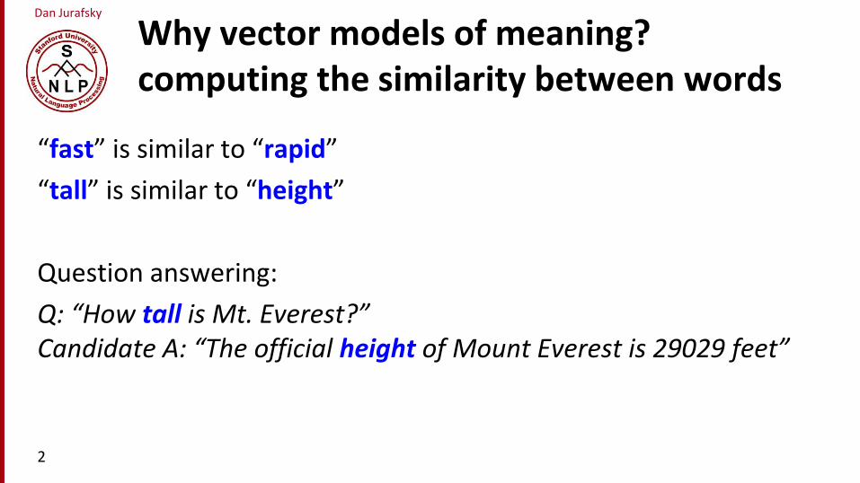
Why vector models of meaning?computing the similarity between words

“fast” is similar to “rapid”

“tall” is similar to “height”

Question answering:

Q: “How tall is Mt. Everest?”Candidate A: “The official height of Mount Everest is 29029 feet”

2

Dan Jurafsky

Word similarity for plagiarism detection

Dan Jurafsky

Word similarity for historical linguistics:semantic change over time

4

Kulkarni, Al-Rfou, Perozzi, Skiena 2015Sagi, Kaufmann Clark 2013

0

5

10

15

20

25

30

35

40

45

dog deer hound

Sem

anti

c B

road

en

ing <1250

Middle 1350-1500

Modern 1500-1710

Dan Jurafsky Distributional models of meaning= vector-space models of meaning = vector semantics

Intuitions: Zellig Harris (1954):

• “oculist and eye-doctor … occur in almost the same environments”

• “If A and B have almost identical environments we say that they are synonyms.”

Firth (1957):

• “You shall know a word by the company it keeps!”5

Dan Jurafsky

Intuition of distributional word similarity

• Nida example:A bottle of tesgüino is on the table

Everybody likes tesgüino

Tesgüino makes you drunk

We make tesgüino out of corn.

• From context words humans can guess tesgüino means

• an alcoholic beverage like beer

• Intuition for algorithm: • Two words are similar if they have similar word contexts.

Dan Jurafsky

Four kinds of vector models

Sparse vector representations

1. Mutual-information weighted word co-occurrence matrices

Dense vector representations:

2. Singular value decomposition (and Latent Semantic Analysis)

3. Neural-network-inspired models (skip-grams, CBOW)

4. Brown clusters

7

Dan Jurafsky

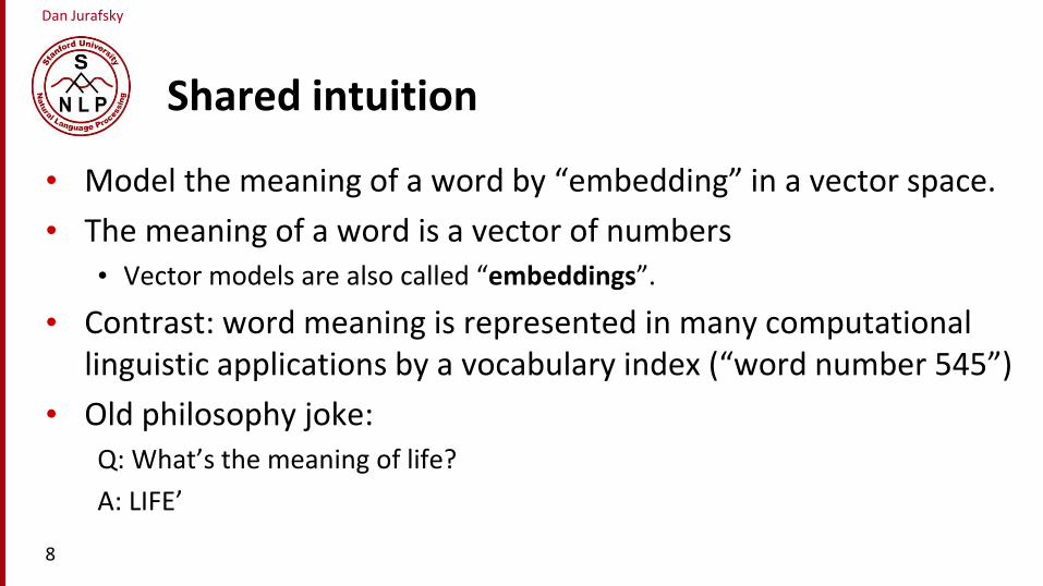
Shared intuition

• Model the meaning of a word by “embedding” in a vector space.

• The meaning of a word is a vector of numbers• Vector models are also called “embeddings”.

• Contrast: word meaning is represented in many computational linguistic applications by a vocabulary index (“word number 545”)

• Old philosophy joke: Q: What’s the meaning of life?

A: LIFE’

8

Dan Jurafsky

AsYouLikeIt TwelfthNight JuliusCaesar HenryV

battle 1 1 8 15

soldier 2 2 12 36

fool 37 58 1 5

clown 6 117 0 0

Reminder: Term-document matrix

• Each cell: count of term t in a document d: tft,d: • Each document is a count vector in ℕv: a column below

9

Dan Jurafsky

Reminder: Term-document matrix

• Two documents are similar if their vectors are similar

10

AsYouLikeIt TwelfthNight JuliusCaesar HenryV

battle 1 1 8 15

soldier 2 2 12 36

fool 37 58 1 5

clown 6 117 0 0

Dan Jurafsky

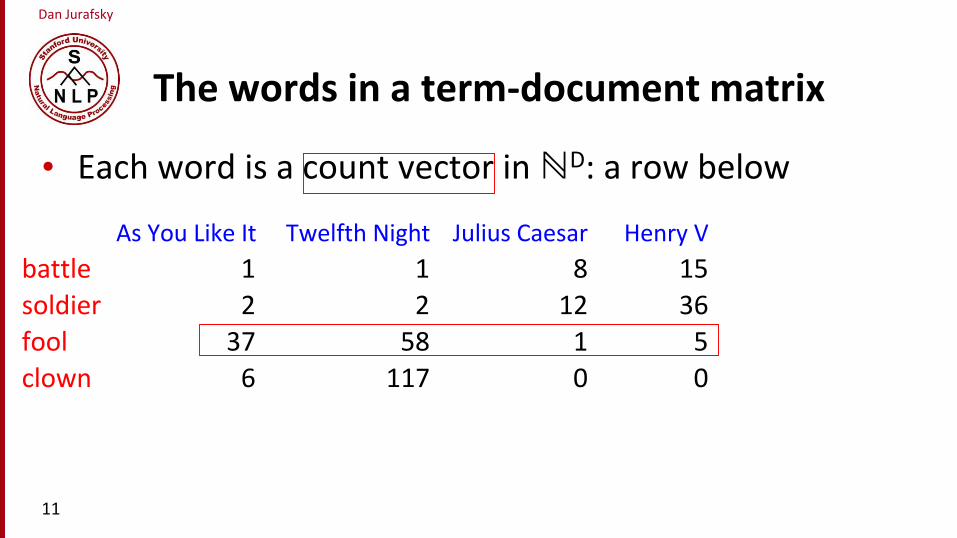
The words in a term-document matrix

• Each word is a count vector in ℕD: a row below

11

AsYouLikeIt TwelfthNight JuliusCaesar HenryV

battle 1 1 8 15

soldier 2 2 12 36

fool 37 58 1 5

clown 6 117 0 0

Dan Jurafsky

The words in a term-document matrix

• Two words are similar if their vectors are similar

12

AsYouLikeIt TwelfthNight JuliusCaesar HenryV

battle 1 1 8 15

soldier 2 2 12 36

fool 37 58 1 5

clown 6 117 0 0

Dan Jurafsky

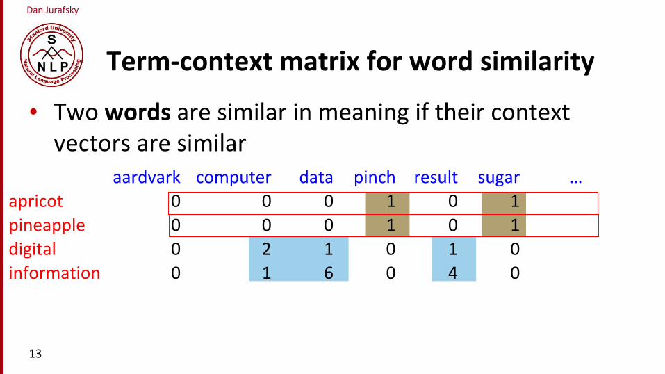
Term-context matrix for word similarity

• Two words are similar in meaning if their context vectors are similar

13

aardvark computer data pinch result sugar …

apricot 0 0 0 1 0 1

pineapple 0 0 0 1 0 1

digital 0 2 1 0 1 0

information 0 1 6 0 4 0

Dan Jurafsky

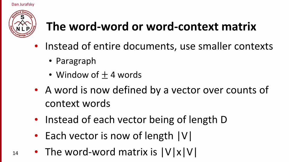
The word-word or word-context matrix

• Instead of entire documents, use smaller contexts

• Paragraph

• Window of ± 4 words

• A word is now defined by a vector over counts of context words

• Instead of each vector being of length D

• Each vector is now of length |V|

• The word-word matrix is |V|x|V|14

Dan Jurafsky

Word-Word matrixSample contexts ± 7 words

15

aardvark computer data pinch result sugar …

apricot 0 0 0 1 0 1

pineapple 0 0 0 1 0 1

digital 0 2 1 0 1 0

information 0 1 6 0 4 0

… …

Dan Jurafsky

Word-word matrix

• We showed only 4x6, but the real matrix is 50,000 x 50,000• So it’s very sparse

• Most values are 0.

• That’s OK, since there are lots of efficient algorithms for sparse matrices.

• The size of windows depends on your goals• The shorter the windows , the more syntactic the representation

± 1-3 very syntacticy

• The longer the windows, the more semantic the representation

± 4-10 more semanticy16

Dan Jurafsky

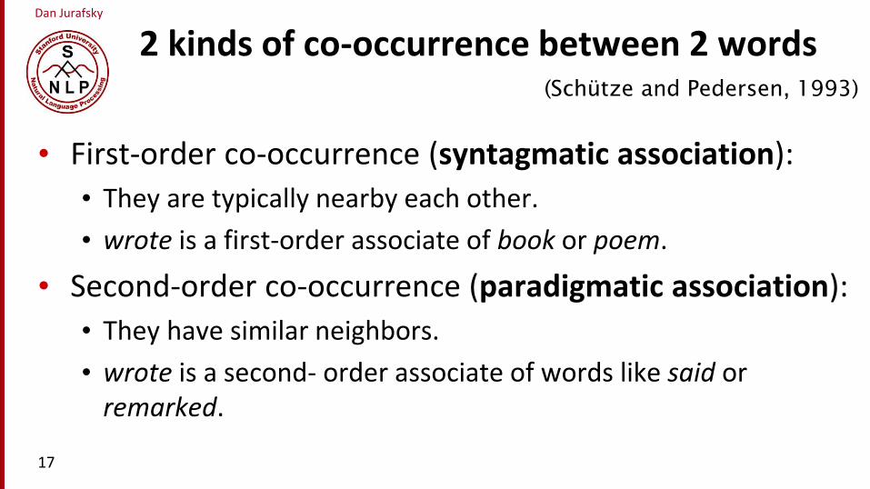
2 kinds of co-occurrence between 2 words

• First-order co-occurrence (syntagmatic association):

• They are typically nearby each other.

• wrote is a first-order associate of book or poem.

• Second-order co-occurrence (paradigmatic association):

• They have similar neighbors.

• wrote is a second- order associate of words like said or remarked.

17

(Schütze and Pedersen, 1993)

Positive Pointwise Mutual Information (PPMI)

Dan Jurafsky

Problem with raw counts

• Raw word frequency is not a great measure of association between words• It’s very skewed

• “the” and “of” are very frequent, but maybe not the most discriminative

• We’d rather have a measure that asks whether a context word is particularly informative about the target word.

• Positive Pointwise Mutual Information (PPMI)

19

Dan Jurafsky

Pointwise Mutual Information

Pointwise mutual information: Do events x and y co-occur more than if they were independent?

PMI between two words: (Church & Hanks 1989)

Do words x and y co-occur more than if they were independent?

PMI 𝑤𝑜𝑟𝑑1, 𝑤𝑜𝑟𝑑2 = log2𝑃(𝑤𝑜𝑟𝑑1, 𝑤𝑜𝑟𝑑2)

𝑃 𝑤𝑜𝑟𝑑1 𝑃(𝑤𝑜𝑟𝑑2)

PMI(X,Y ) = log2

P(x,y)P(x)P(y)

Dan Jurafsky

Positive Pointwise Mutual Information

• PMI ranges from −∞ to +∞

• But the negative values are problematic

• Things are co-occurring less than we expect by chance

• Unreliable without enormous corpora• Imagine w1 and w2 whose probability is each 10-6

• Hard to be sure p(w1,w2) is significantly different than 10-12

• Plus it’s not clear people are good at “unrelatedness”

• So we just replace negative PMI values by 0

• Positive PMI (PPMI) between word1 and word2:

PPMI 𝑤𝑜𝑟𝑑1, 𝑤𝑜𝑟𝑑2 = max log2𝑃(𝑤𝑜𝑟𝑑1, 𝑤𝑜𝑟𝑑2)

𝑃 𝑤𝑜𝑟𝑑1 𝑃(𝑤𝑜𝑟𝑑2), 0

Dan Jurafsky

Computing PPMI on a term-context matrix

• Matrix F with W rows (words) and C columns (contexts)

• fij is # of times wi occurs in context cj

22

pij =fij

fijj=1

C

åi=1

W

åpi* =

fijj=1

C

å

fijj=1

C

åi=1

W

å

p* j =

fiji=1

W

å

fijj=1

C

åi=1

W

å

pmiij = log2

pij

pi*p* j

ppmiij =pmiij if pmiij > 0

0 otherwise

ìíï

îï

Dan Jurafsky

p(w=information,c=data) =

p(w=information) =

p(c=data) =

23

p(w,context) p(w)

computer data pinch result sugar

apricot 0.00 0.00 0.05 0.00 0.05 0.11

pineapple 0.00 0.00 0.05 0.00 0.05 0.11

digital 0.11 0.05 0.00 0.05 0.00 0.21

information 0.05 0.32 0.00 0.21 0.00 0.58

p(context) 0.16 0.37 0.11 0.26 0.11

= .326/19

11/19 = .58

7/19 = .37

pij =fij

fijj=1

C

åi=1

W

å

p(wi ) =

fijj=1

C

å

Np(c j ) =

fiji=1

W

å

N

Dan Jurafsky

24

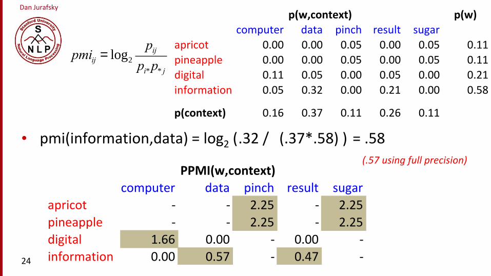
pmiij = log2

pij

pi*p* j

• pmi(information,data) = log2 (

p(w,context) p(w)

computer data pinch result sugar

apricot 0.00 0.00 0.05 0.00 0.05 0.11

pineapple 0.00 0.00 0.05 0.00 0.05 0.11

digital 0.11 0.05 0.00 0.05 0.00 0.21

information 0.05 0.32 0.00 0.21 0.00 0.58

p(context) 0.16 0.37 0.11 0.26 0.11

PPMI(w,context)

computer data pinch result sugar

apricot - - 2.25 - 2.25

pineapple - - 2.25 - 2.25

digital 1.66 0.00 - 0.00 -

information 0.00 0.57 - 0.47 -

.32 / (.37*.58) ) = .58(.57 using full precision)

Dan Jurafsky

Weighting PMI

• PMI is biased toward infrequent events

• Very rare words have very high PMI values

• Two solutions:

• Give rare words slightly higher probabilities

• Use add-one smoothing (which has a similar effect)

25

Dan Jurafsky Weighting PMI: Giving rare context words slightly higher probability

• Raise the context probabilities to 𝛼 = 0.75:

• This helps because 𝑃𝛼 𝑐 > 𝑃 𝑐 for rare c

• Consider two events, P(a) = .99 and P(b)=.01

• 𝑃𝛼 𝑎 =.99.75

.99.75+.01.75= .97 𝑃𝛼 𝑏 =

.01.75

.01.75+.01.75= .0326

Dan Jurafsky

Use Laplace (add-1) smoothing

27

Dan Jurafsky

28

Add-2SmoothedCount(w,context)

computer data pinch result sugar

apricot 2 2 3 2 3

pineapple 2 2 3 2 3

digital 4 3 2 3 2

information 3 8 2 6 2

p(w,context)[add-2] p(w)

computer data pinch result sugar

apricot 0.03 0.03 0.05 0.03 0.05 0.20

pineapple 0.03 0.03 0.05 0.03 0.05 0.20

digital 0.07 0.05 0.03 0.05 0.03 0.24

information 0.05 0.14 0.03 0.10 0.03 0.36

p(context) 0.19 0.25 0.17 0.22 0.17

Dan Jurafsky

PPMI versus add-2 smoothed PPMI

29

PPMI(w,context)[add-2]

computer data pinch result sugar

apricot 0.00 0.00 0.56 0.00 0.56

pineapple 0.00 0.00 0.56 0.00 0.56

digital 0.62 0.00 0.00 0.00 0.00

information 0.00 0.58 0.00 0.37 0.00

PPMI(w,context)

computer data pinch result sugar

apricot - - 2.25 - 2.25

pineapple - - 2.25 - 2.25

digital 1.66 0.00 - 0.00 -

information 0.00 0.57 - 0.47 -

Measuring similarity: the cosine

Dan Jurafsky

Measuring similarity

• Given 2 target words v and w

• We’ll need a way to measure their similarity.

• Most measure of vectors similarity are based on the:

• Dot product or inner product from linear algebra

• High when two vectors have large values in same dimensions.

• Low (in fact 0) for orthogonal vectors with zeros in complementary distribution31

Dan Jurafsky

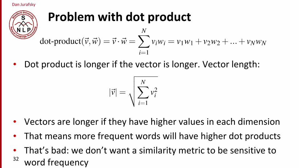
Problem with dot product

• Dot product is longer if the vector is longer. Vector length:

• Vectors are longer if they have higher values in each dimension

• That means more frequent words will have higher dot products

• That’s bad: we don’t want a similarity metric to be sensitive to word frequency32

Dan Jurafsky

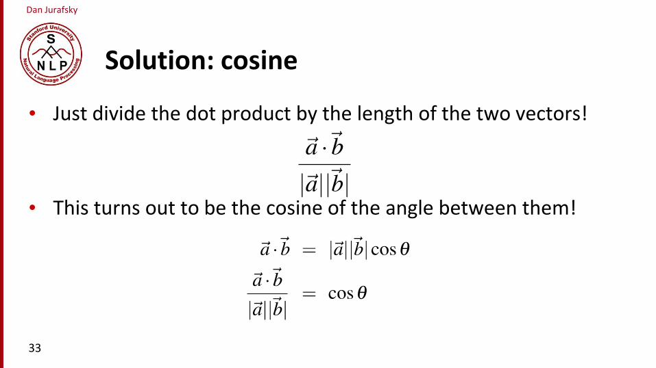
Solution: cosine

• Just divide the dot product by the length of the two vectors!

• This turns out to be the cosine of the angle between them!

33

Dan Jurafsky

Cosine for computing similarity

cos(v,w) =v ·w

v w=v

v·w

w=

viwii=1

N

å

vi2

i=1

N

å wi2

i=1

N

å

Dot product Unit vectors

vi is the PPMI value for word v in context iwi is the PPMI value for word w in context i.

Cos(v,w) is the cosine similarity of v and w

Sec. 6.3

Dan Jurafsky

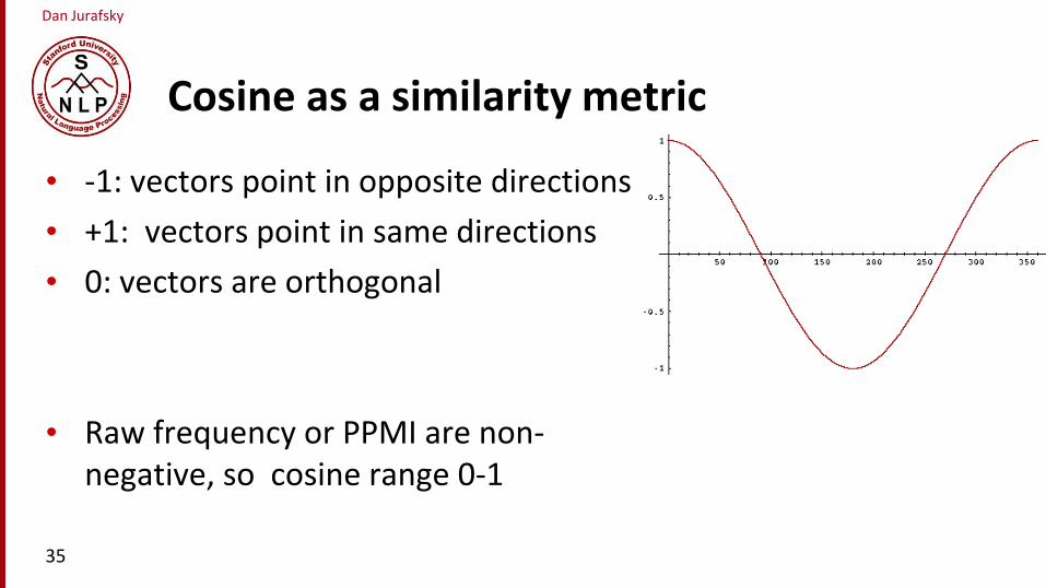
Cosine as a similarity metric

• -1: vectors point in opposite directions

• +1: vectors point in same directions

• 0: vectors are orthogonal

• Raw frequency or PPMI are non-negative, so cosine range 0-1

35

Dan Jurafsky

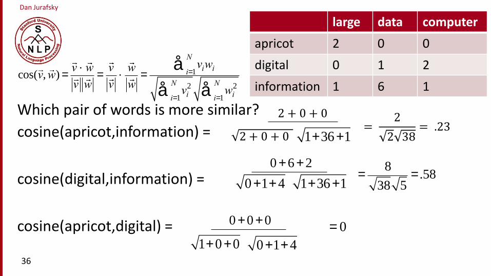
large data computer

apricot 2 0 0

digital 0 1 2

information 1 6 1

36

Which pair of words is more similar?

cosine(apricot,information) =

cosine(digital,information) =

cosine(apricot,digital) =

cos(v,w) =v ·w

v w=v

v·w

w=

viwii=1

N

å

vi2

i=1

N

å wi2

i=1

N

å

1+ 0+0

1+36+1

1+36+1

0+1+ 4

0+1+ 4

0 + 6 + 2

0 + 0 + 0

=8

38 5= .58

= 0

2 + 0 + 0

2 + 0 + 0=

2

2 38= .23

Dan Jurafsky

Visualizing vectors and angles

1 2 3 4 5 6 7

1

2

3

digital

apricotinformation

Dim

ensi

on

1:

‘la

rge’

Dimension 2: ‘data’37

large data

apricot 2 0

digital 0 1

information 1 6

Dan Jurafsky

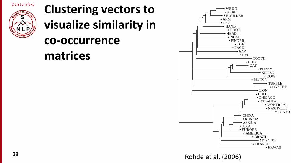
Clustering vectors to visualize similarity in co-occurrence matrices

Rohde, Gonnerman, Plaut Modeling Word Meaning Using Lexical Co-Occurrence

HEAD

HANDFACE

DOG

AMERICA

CAT

EYE

EUROPE

FOOT

CHINAFRANCE

CHICAGO

ARM

FINGER

NOSE

LEG

RUSSIA

MOUSE

AFRICA

ATLANTA

EAR

SHOULDER

ASIA

COW

BULL

PUPPYLION

HAWAII

MONTREAL

TOKYO

TOE

MOSCOW

TOOTH

NASHVILLE

BRAZIL

WRIST

KITTEN

ANKLE

TURTLE

OYSTER

Figure 8: Multidimensional scaling for three noun classes.

WRISTANKLE

SHOULDERARMLEG

HANDFOOT

HEADNOSEFINGER

TOEFACE

EAREYE

TOOTHDOGCAT

PUPPYKITTEN

COWMOUSE

TURTLEOYSTER

LIONBULLCHICAGOATLANTA

MONTREALNASHVILLE

TOKYOCHINA

RUSSIAAFRICAASIAEUROPE

AMERICABRAZIL

MOSCOWFRANCE

HAWAII

Figure 9: Hierarchical clustering for three noun classes using distances based on vector correlations.

20

38 Rohde et al. (2006)

Dan Jurafsky

Other possible similarity measures

Measuring similarity: the cosine

Dan Jurafsky

Using syntax to define a word’s context

• Zellig Harris (1968)

“The meaning of entities, and the meaning of grammatical relations among them, is related to the restriction of combinations of these entities relative to other entities”

• Two words are similar if they have similar syntactic contexts

Duty and responsibility have similar syntactic distribution:

Modified by adjectives

additional, administrative, assumed, collective, congressional, constitutional …

Objects of verbs assert, assign, assume, attend to, avoid, become, breach..

Dan Jurafsky

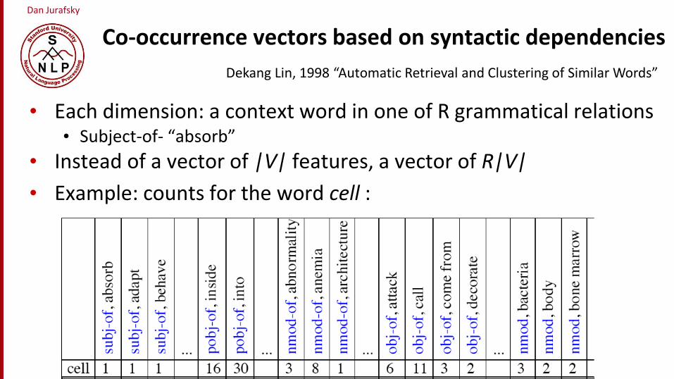
Co-occurrence vectors based on syntactic dependencies

• Each dimension: a context word in one of R grammatical relations• Subject-of- “absorb”

• Instead of a vector of |V| features, a vector of R|V|

• Example: counts for the word cell :

Dekang Lin, 1998 “Automatic Retrieval and Clustering of Similar Words”

Dan Jurafsky

Syntactic dependencies for dimensions

• Alternative (Padó and Lapata 2007):• Instead of having a |V| x R|V| matrix

• Have a |V| x |V| matrix

• But the co-occurrence counts aren’t just counts of words in a window

• But counts of words that occur in one of R dependencies (subject, object, etc).

• So M(“cell”,”absorb”) = count(subj(cell,absorb)) + count(obj(cell,absorb)) + count(pobj(cell,absorb)), etc.

43

Dan Jurafsky

PMI applied to dependency relations

• “Drink it” more common than “drink wine”

• But “wine” is a better “drinkable” thing than “it”

Object of “drink” Count PMI

it 3 1.3

anything 3 5.2

wine 2 9.3

tea 2 11.8

liquid 2 10.5

Hindle, Don. 1990. Noun Classification from Predicate-Argument Structure. ACL

Object of “drink” Count PMI

tea 2 11.8

liquid 2 10.5

wine 2 9.3

anything 3 5.2

it 3 1.3

Dan Jurafsky

Alternative to PPMI for measuring association

• tf-idf (that’s a hyphen not a minus sign)

• The combination of two factors• Term frequency (Luhn 1957): frequency of the word (can be logged)

• Inverse document frequency (IDF) (Sparck Jones 1972)

• N is the total number of documents

• dfi = “document frequency of word i”

• = # of documents with word I

• wij = word i in document j

wij=tfij idfi45

idfi

= logN

dfi

æ

è

çç

ö

ø

÷÷

Dan Jurafsky

tf-idf not generally used for word-word similarity

• But is by far the most common weighting when we are considering the relationship of words to documents

46

Dense Vectors

Dan Jurafsky

Sparse versus dense vectors

• PPMI vectors are

• long (length |V|= 20,000 to 50,000)

• sparse (most elements are zero)

• Alternative: learn vectors which are

• short (length 200-1000)

• dense (most elements are non-zero)

48

Dan Jurafsky

Sparse versus dense vectors

• Why dense vectors?

• Short vectors may be easier to use as features in machine learning (less weights to tune)

• Dense vectors may generalize better than storing explicit counts

• They may do better at capturing synonymy:

• car and automobile are synonyms; but are represented as distinct dimensions; this fails to capture similarity between a word with car as a neighbor and a word with automobile as a neighbor

49

Dan Jurafsky

Three methods for getting short dense vectors

• Singular Value Decomposition (SVD)

• A special case of this is called LSA – Latent Semantic Analysis

• “Neural Language Model”-inspired predictive models

• skip-grams and CBOW

• Brown clustering

50

Evaluating similarity

Dan Jurafsky

Evaluating similarity

• Extrinsic (task-based, end-to-end) Evaluation:• Question Answering

• Spell Checking

• Essay grading

• Intrinsic Evaluation:• Correlation between algorithm and human word similarity ratings

• Wordsim353: 353 noun pairs rated 0-10. sim(plane,car)=5.77

• Taking TOEFL multiple-choice vocabulary tests

• Levied is closest in meaning to:

imposed, believed, requested, correlated

Dan Jurafsky

Summary

• Distributional (vector) models of meaning

• Sparse (PPMI-weighted word-word co-occurrence matrices)

• Dense:

• Word-word SVD 50-2000 dimensions

• Skip-grams and CBOW

• Brown clusters 5-20 binary dimensions.

53

Dan Jurafsky

The remaining material is optionaland won’t be on the final exam.

54

Dense Vectors via SVD

Dan Jurafsky

Intuition

• Approximate an N-dimensional dataset using fewer dimensions

• By first rotating the axes into a new space

• In which the highest order dimension captures the most variance in the original dataset

• And the next dimension captures the next most variance, etc.

• Many such (related) methods:• PCA – principle components analysis

• Factor Analysis

• SVD56

Dan Jurafsky

57

Dimensionality reduction

Dan Jurafsky

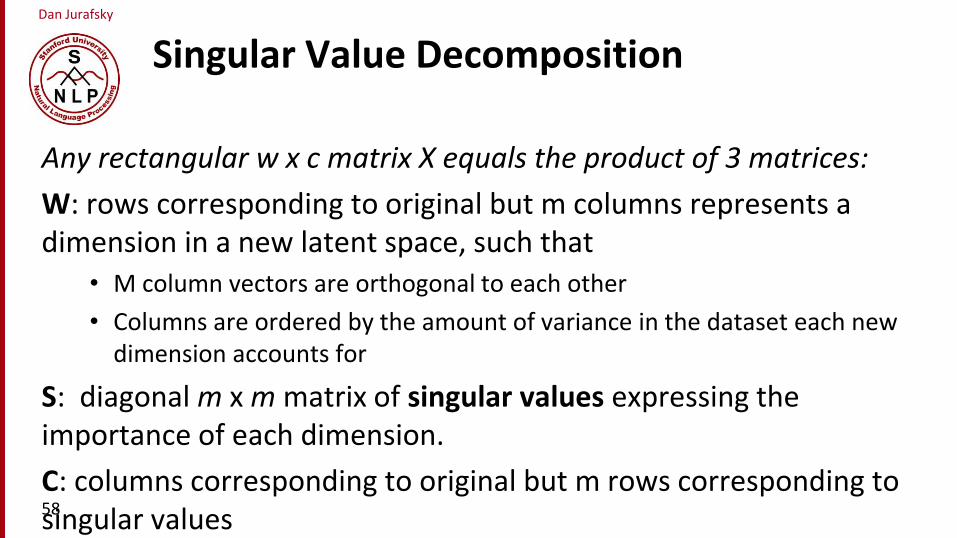
Singular Value Decomposition

58

Any rectangular w x c matrix X equals the product of 3 matrices:

W: rows corresponding to original but m columns represents a dimension in a new latent space, such that

• M column vectors are orthogonal to each other

• Columns are ordered by the amount of variance in the dataset each new dimension accounts for

S: diagonal m x m matrix of singular values expressing the importance of each dimension.

C: columns corresponding to original but m rows corresponding to singular values

Dan Jurafsky

Singular Value Decomposition

59 Landuaer and Dumais 1997

Dan Jurafsky

SVD applied to term-document matrix:Latent Semantic Analysis

• If instead of keeping all m dimensions, we just keep the top k singular values. Let’s say 300.

• The result is a least-squares approximation to the original X

• But instead of multiplying, we’ll just make use of W.

• Each row of W:• A k-dimensional vector

• Representing word W

60 k/

/k

/k

/k

Deerwester et al (1988)

Dan Jurafsky

LSA more details

• 300 dimensions are commonly used

• The cells are commonly weighted by a product of two weights• Local weight: Log term frequency

• Global weight: either idf or an entropy measure

61

Dan Jurafsky

Let’s return to PPMI word-word matrices

• Can we apply to SVD to them?

62

Dan Jurafsky

SVD applied to term-term matrix

63 (I’m simplifying here by assuming the matrix has rank |V|)

Dan Jurafsky

Truncated SVD on term-term matrix

64

Dan Jurafsky

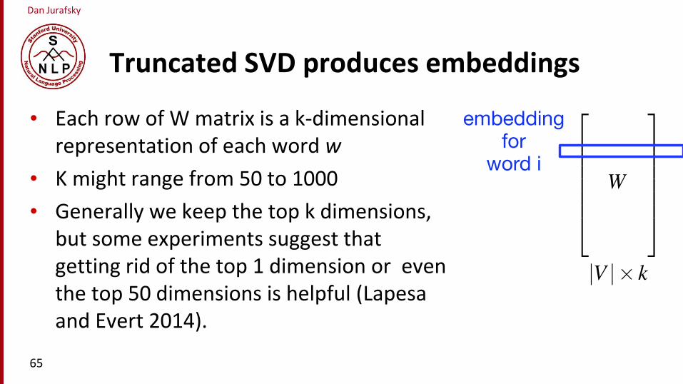
Truncated SVD produces embeddings

65

• Each row of W matrix is a k-dimensional representation of each word w

• K might range from 50 to 1000

• Generally we keep the top k dimensions, but some experiments suggest that getting rid of the top 1 dimension or even the top 50 dimensions is helpful (Lapesaand Evert 2014).

Dan Jurafsky

Embeddings versus sparse vectors

• Dense SVD embeddings sometimes work better than sparse PPMI matrices at tasks like word similarity• Denoising: low-order dimensions may represent unimportant

information

• Truncation may help the models generalize better to unseen data.

• Having a smaller number of dimensions may make it easier for classifiers to properly weight the dimensions for the task.

• Dense models may do better at capturing higher order co-occurrence.

66

Embeddings inspired by neural language models:

skip-grams and CBOW

Dan Jurafsky Prediction-based models:An alternative way to get dense vectors

• Skip-gram (Mikolov et al. 2013a) CBOW (Mikolov et al. 2013b)

• Learn embeddings as part of the process of word prediction.

• Train a neural network to predict neighboring words• Inspired by neural net language models.

• In so doing, learn dense embeddings for the words in the training corpus.

• Advantages:• Fast, easy to train (much faster than SVD)

• Available online in the word2vec package

• Including sets of pretrained embeddings!68

Dan Jurafsky

Skip-grams

• Predict each neighboring word

• in a context window of 2C words

• from the current word.

• So for C=2, we are given word wt and predicting these 4 words:

69

Dan Jurafsky

Skip-grams learn 2 embeddingsfor each w

input embedding v, in the input matrix W

• Column i of the input matrix W is the 1× d embedding vi for word i in the vocabulary.

output embedding v′, in output matrix W’

• Row i of the output matrix W′ is a d × 1 vector embedding v′i for word i in the vocabulary.

70

Dan Jurafsky

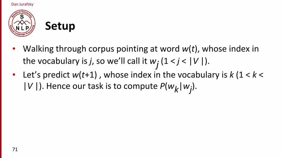
Setup

• Walking through corpus pointing at word w(t), whose index in

the vocabulary is j, so we’ll call it wj (1 < j < |V |).

• Let’s predict w(t+1) , whose index in the vocabulary is k (1 < k < |V |). Hence our task is to compute P(wk|wj).

71

Dan Jurafsky

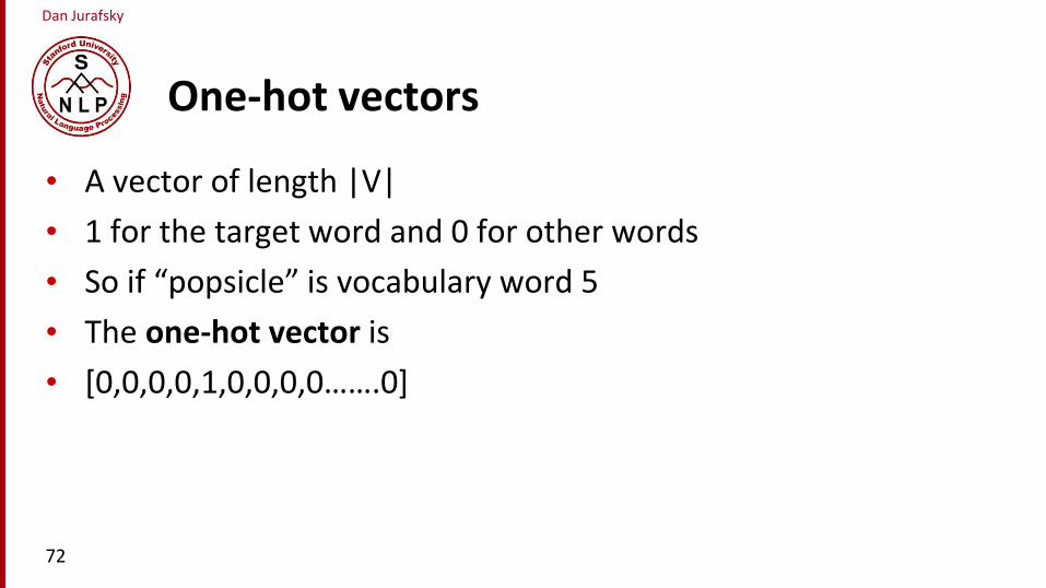
One-hot vectors

• A vector of length |V|

• 1 for the target word and 0 for other words

• So if “popsicle” is vocabulary word 5

• The one-hot vector is

• [0,0,0,0,1,0,0,0,0…….0]

72

Dan Jurafsky

73

Skip-gram

Dan Jurafsky

74

Skip-gramh = vj

o = W’h

o = W’h

Dan Jurafsky

75

Skip-gram

h = vj

o = W’hok = v’khok = v’k∙vj

Dan Jurafsky

Turning outputs into probabilities

• ok = v’k∙vj

• We use softmax to turn into probabilities

76

Dan Jurafsky

Embeddings from W and W’

• Since we have two embeddings, vj and v’j for each word wj• We can either:

• Just use vj

• Sum them

• Concatenate them to make a double-length embedding

77

Dan Jurafsky

But wait; how do we learn the embeddings?

78

Dan Jurafsky

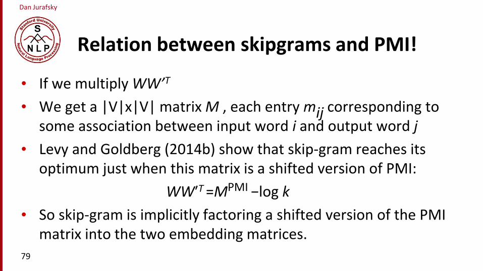
Relation between skipgrams and PMI!

• If we multiply WW’T

• We get a |V|x|V| matrix M , each entry mij corresponding to some association between input word i and output word j

• Levy and Goldberg (2014b) show that skip-gram reaches its optimum just when this matrix is a shifted version of PMI:

WW′T =MPMI −log k

• So skip-gram is implicitly factoring a shifted version of the PMI matrix into the two embedding matrices.

79

Dan Jurafsky

CBOW (Continuous Bag of Words)

80

Dan Jurafsky

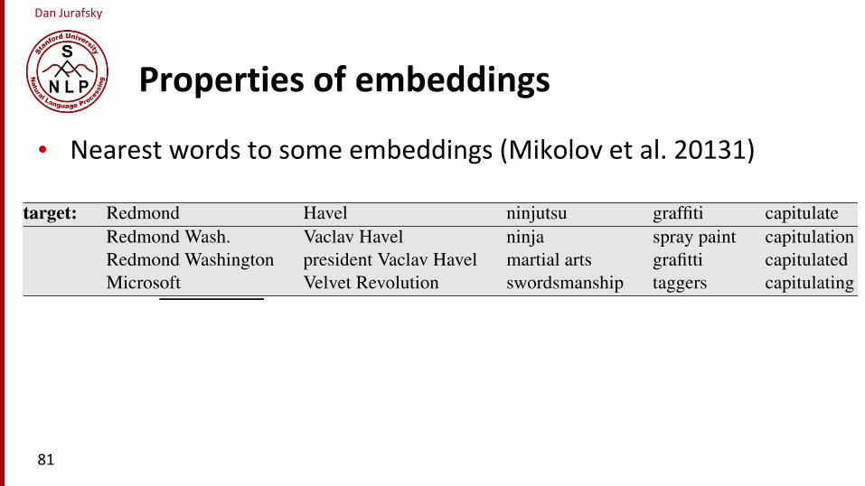
Properties of embeddings

81

• Nearest words to some embeddings (Mikolov et al. 20131)

Dan Jurafsky

Embeddings capture relational meaning!

vector(‘king’) - vector(‘man’) + vector(‘woman’) ≈ vector(‘queen’)

vector(‘Paris’) - vector(‘France’) + vector(‘Italy’) ≈ vector(‘Rome’)

82

Brown clustering

Dan Jurafsky

Brown clustering

• An agglomerative clustering algorithm that clusters words based on which words precede or follow them

• These word clusters can be turned into a kind of vector

• We’ll give a very brief sketch here.

84

Dan Jurafsky

Brown clustering algorithm

• Each word is initially assigned to its own cluster.

• We now consider consider merging each pair of clusters. Highest quality merge is chosen.• Quality = merges two words that have similar probabilities of preceding

and following words

• (More technically quality = smallest decrease in the likelihood of the corpus according to a class-based language model)

• Clustering proceeds until all words are in one big cluster.

85

Dan Jurafsky

Brown Clusters as vectors

• By tracing the order in which clusters are merged, the model builds a binary tree from bottom to top.

• Each word represented by binary string = path from root to leaf

• Each intermediate node is a cluster

• Chairman is 0010, “months” = 01, and verbs = 1

86

Brown Algorithm

• Words merged according to contextual

similarity

• Clusters are equivalent to bit-string prefixes

• Prefix length determines the granularity of

the clustering

011

president

walk

run sprintchairman

CEO November October

0 1

00 01

00110010

001

10 11

000 100 101010

Dan Jurafsky

Brown cluster examples

87

Dan Jurafsky

Class-based language model

• Suppose each word was in some class ci:

88

19.7 • BROWN CLUSTERING 19

Figure19.15 Vector offsets showing relational properties of the vector space, shown byprojectingvectorsontotwodimensionsusingPCA.Intheleft panel, ’king’ -’man’+ ’woman’iscloseto ’queen’. In theright, weseetheway offsetsseemtocapturegrammatical number.(Mikolov et al., 2013b).

19.7 BrownClustering

Brown clustering (Brownet al., 1992) isanagglomerativeclustering algorithm forBrownclustering

derivingvector representationsof wordsby clusteringwordsbasedontheir associa-tionswith theprecedingor followingwords.The algorithm makes use of the class-based language model (Brown et al.,class-based

languagemodel

1992),amodel inwhicheachwordw2 V belongstoaclassc2 CwithaprobabilityP(w|c). Class based LMsassigns a probability to a pair of wordswi−1 andwi bymodeling thetransition betweenclasses rather thanbetweenwords:

P(wi |wi−1) = P(ci |ci−1)P(wi |ci) (19.32)

Theclass-basedLM canbeusedtoassignaprobability toanentirecorpusgivenaparticularly clusteringC asfollows:

P(corpus|C) =

nY

i−1

P(ci |ci−1)P(wi |ci) (19.33)

Class-based language models are generally not used as a language model for ap-plications likemachine translation or speech recognition because they don’t workaswell as standard n-gramsor neural languagemodels. But they are an importantcomponent inBrownclustering.Brown clustering is a hierarchical clustering algorithm. Let’sconsider a naive

(albeit inefficient) versionof thealgorithm:

1. Eachword isinitially assigned to itsowncluster.

2. We now consider consider merging each pair of clusters. The pair whosemerger resultsin thesmallest decreasein thelikelihoodof thecorpus(accord-ing to theclass-based languagemodel) ismerged.

3. Clustering proceedsuntil all wordsare inonebigcluster.

Twowordsarethusmost likely tobeclustered if they havesimilar probabilitiesfor preceding and followingwords, leading tomorecoherent clusters. Theresult isthat wordswill bemerged if they arecontextually similar.By tracing theorder inwhichclustersaremerged, themodel buildsabinary tree

from bottom to top, in which the leavesare thewords in the vocabulary, and eachintermediate node in the tree represents the cluster that is formed by merging itschildren. Fig. 19.16 showsaschematic view of apart of atree.

19.7 • BROWN CLUSTERING 19

Figure19.15 Vector offsets showing relational properties of the vector space, shown byprojectingvectorsontotwodimensionsusingPCA. Intheleft panel, ’king’ -’man’ + ’woman’isclose to ’queen’. In theright, weseetheway offsetsseem tocapturegrammatical number.(Mikolov et al., 2013b).

19.7 BrownClustering

Brown cluster ing (Brownet al., 1992) isan agglomerativeclustering algorithm forBrowncluster ing

derivingvector representationsof wordsby clusteringwordsbasedon their associa-tionswith thepreceding or followingwords.The algorithm makes use of the class-based language model (Brown et al.,class-based

languagemodel

1992),amodel inwhicheachwordw2 V belongstoaclassc2 Cwith aprobabilityP(w|c). Class based LMs assigns a probability to a pair of wordswi− 1 andwi bymodeling the transition between classes rather than between words:

P(wi |wi− 1) = P(ci |ci− 1)P(wi |ci) (19.32)

Theclass-based LM canbeused toassign aprobability toanentirecorpusgivenaparticularly clusteringC asfollows:

P(corpus|C) =

nY

i− 1

P(ci |ci− 1)P(wi |ci) (19.33)

Class-based language models are generally not used as a language model for ap-plications likemachine translation or speech recognition because they don’t workaswell as standard n-gramsor neural language models. But they are an importantcomponent in Brownclustering.Brown clustering is a hierarchical clustering algorithm. Let’s consider a naive

(albeit inefficient) version of thealgorithm:

1. Eachword is initially assigned to itsowncluster.

2. We now consider consider merging each pair of clusters. The pair whosemerger results in thesmallest decrease in thelikelihoodof thecorpus(accord-ing to theclass-based languagemodel) ismerged.

3. Clustering proceedsuntil all wordsare in onebigcluster.

Twowordsare thusmost likely tobeclustered if they havesimilar probabilitiesfor preceding and followingwords, leading tomorecoherent clusters. The result isthat wordswill bemerged if they arecontextually similar.By tracing theorder inwhich clustersaremerged, themodel buildsabinary tree

from bottom to top, in which the leaves are the words in the vocabulary, and eachintermediate node in the tree represents the cluster that is formed by merging itschildren. Fig. 19.16 showsaschematic view of apart of a tree.