Fast Random Walk with Restart and Its Applications Hanghang Tong, Christos Faloutsos and Jia-Yu...
46
Fast Random Walk with Restart and Its Applications Hanghang Tong, Christos Faloutsos and Jia-Yu (Tim) Pan
-
date post
21-Dec-2015 -
Category
Documents
-
view
228 -
download
2
Transcript of Fast Random Walk with Restart and Its Applications Hanghang Tong, Christos Faloutsos and Jia-Yu...

Fast Random Walk with Restart and Its Applications
Hanghang Tong, Christos Faloutsos and Jia-Yu (Tim) Pan
ICDM 2006 Dec. 18-22, HongKong

2
Motivating Questions
• Q: How to measure the relevance?
• A: Random walk with restart
• Q: How to do it efficiently?
• A: This talk tries to answer!

3
1
4
3
2
56
7
910
8
11
12
Random walk with restart

4
Random walk with restart
Node 4
Node 1Node 2Node 3Node 4Node 5Node 6Node 7Node 8Node 9Node 10Node 11Node 12
0.130.100.130.220.130.050.050.080.040.030.040.02
1
4
3
2
56
7
910
811
120.13
0.10
0.13
0.13
0.05
0.05
0.08
0.04
0.02
0.04
0.03
Ranking vector More red, more relevant
Nearby nodes, higher scores
4r

5
Automatic Image Caption• Q
…
Sea Sun Sky Wave{ } { }Cat Forest Grass Tiger
{?, ?, ?,}
?A: RWR! [Pan KDD2004]
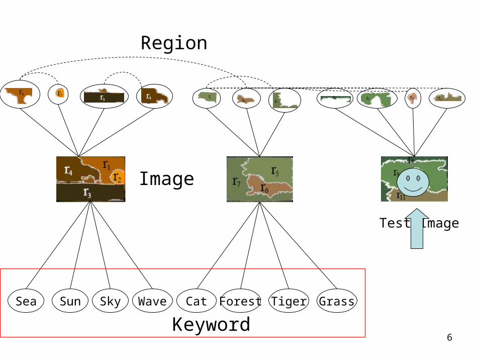
6
Test Image
Sea Sun Sky Wave Cat Forest Tiger Grass
Image
Keyword
Region
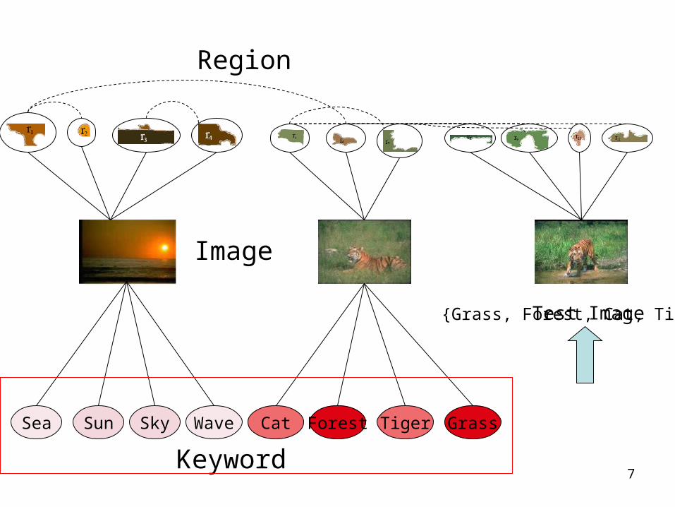
7
Test Image
Sea Sun Sky Wave Cat Forest Tiger Grass
Image
Keyword
Region
{Grass, Forest, Cat, Tiger}

8
Neighborhood Formulation
ICDM
KDD
SDM
Philip S. Yu
IJCAI
NIPS
AAAI M. Jordan
Ning Zhong
R. Ramakrishnan
…
…
… …
Conference Author
A: RWR! [Sun ICDM2005]
Q: what is most related conference to ICDM
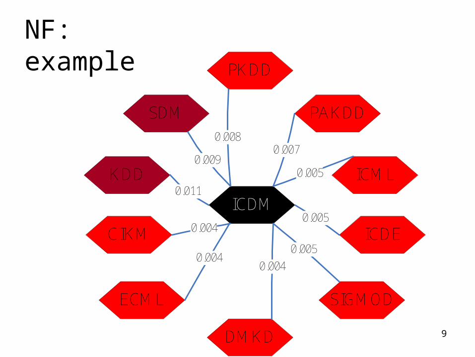
9
NF: example
ICDM
KDD
SDM
ECML
PKDD
PAKDD
CIKM
DMKD
SIGMOD
ICML
ICDE
0.009
0.011
0.0080.007
0.005
0.005
0.005
0.0040.004
0.004

10
Center-Piece Subgraph(CePS)
A C
B
A C
B
?
Original GraphBlack: query nodes
CePS
Q
A: RWR! [Tong KDD 2006]

11
CePS: Example
R. Agrawal Jiawei Han
V. Vapnik M. Jordan
H.V. Jagadish
Laks V.S. Lakshmanan
Heikki Mannila
Christos Faloutsos
Padhraic Smyth
Corinna Cortes
15 1013
1 1
6
1 1
4 Daryl Pregibon
10
2
11
3
16
12
Other Applications
• Content-based Image Retrieval [He]
• Personalized PageRank [Jeh], [Widom], [Haveliwala]
• Anomaly Detection (for node; link) [Sun]
• Link Prediction [Getoor], [Jensen]
• Semi-supervised Learning [Zhu], [Zhou]
• …
13
Roadmap
• Background– RWR: Definitions– RWR: Algorithms
• Basic Idea• FastRWR
– Pre-Compute Stage– On-Line Stage
• Experimental Results• Conclusion

14
Computing RWR
1
43
2
5 6
7
9 10
811
12
0.13 0 1/3 1/3 1/3 0 0 0 0 0 0 0 0
0.10 1/3 0 1/3 0 0 0 0 1/4 0 0 0
0.13
0.22
0.13
0.050.9
0.05
0.08
0.04
0.03
0.04
0.02
0
1/3 1/3 0 1/3 0 0 0 0 0 0 0 0
1/3 0 1/3 0 1/4 0 0 0 0 0 0 0
0 0 0 1/3 0 1/2 1/2 1/4 0 0 0 0
0 0 0 0 1/4 0 1/2 0 0 0 0 0
0 0 0 0 1/4 1/2 0 0 0 0 0 0
0 1/3 0 0 1/4 0 0 0 1/2 0 1/3 0
0 0 0 0 0 0 0 1/4 0 1/3 0 0
0 0 0 0 0 0 0 0 1/2 0 1/3 1/2
0 0 0 0 0 0 0 1/4 0 1/3 0 1/2
0 0 0 0 0 0 0 0 0 1/3 1/3 0
0.13 0
0.10 0
0.13 0
0.22
0.13 0
0.05 00.1
0.05 0
0.08 0
0.04 0
0.03 0
0.04 0
2 0
1
0.0
n x n n x 1n x 1
Ranking vector Starting vectorAdjacent matrix
1
(1 )i i ir cWr c e
Restart p
15
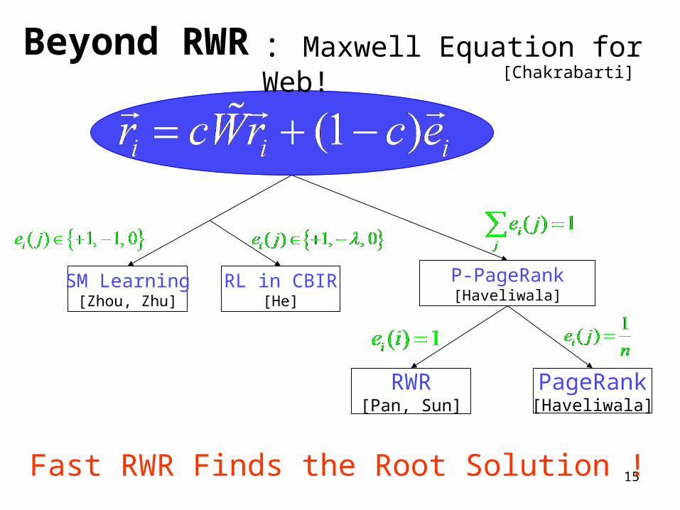
Beyond RWR
P-PageRank[Haveliwala]
PageRank[Haveliwala]
RWR[Pan, Sun]
SM Learning[Zhou, Zhu]
RL in CBIR[He]
Fast RWR Finds the Root Solution !
: Maxwell Equation for Web![Chakrabarti]

16
• Q: Given query i, how to solve it?
0 1/3 1/3 1/3 0 0 0 0 0 0 0 0
1/3 0 1/3 0 0 0 0 1/4 0 0 0 0
1/3 1/3 0 1/3 0 0 0 0 0 0 0 0
1/3 0 1/3 0 1/4
0.9
0 0 0 0 0 0 0
0 0 0 1/3 0 1/2 1/2 1/4 0 0 0 0
0 0 0 0 1/4 0 1/2 0 0 0 0 0
0 0 0 0 1/4 1/2 0 0 0 0 0 0
0 1/3 0 0 1/4 0 0 0 1/2 0 1/3 0
0 0 0 0 0 0 0 1/4 0 1/3 0 0
0 0 0 0 0 0 0 0 1/2 0 1/3 1/2
0 0 0 0 0
0
0
0
0
00.1
0
0
0
0
0 0 1/4 0 1/3 0 1/2 0
0 0 0 0 0 0 0 0 0 1/3 1/3
1
0 0
??

17
1
43
2
5 6
7
9 10
8 11
120.130.10
0.13
0.130.05
0.05
0.08
0.04
0.02
0.04
0.03
OntheFly: 0 1/3 1/3 1/3 0 0 0 0 0 0 0 0
1/3 0 1/3 0 0 0 0 1/4 0 0 0 0
1/3 1/3 0 1/3 0 0 0 0 0 0 0 0
1/3 0 1/3 0 1/4
0.9
0 0 0 0 0 0 0
0 0 0 1/3 0 1/2 1/2 1/4 0 0 0 0
0 0 0 0 1/4 0 1/2 0 0 0 0 0
0 0 0 0 1/4 1/2 0 0 0 0 0 0
0 1/3 0 0 1/4 0 0 0 1/2 0 1/3 0
0 0 0 0 0 0 0 1/4 0 1/3 0 0
0 0 0 0 0 0 0 0 1/2 0 1/3 1/2
0 0 0 0 0
0
0
0
0
00.1
0
0
0
0
0 0 1/4 0 1/3 0 1/2 0
0 0 0 0 0 0 0 0 0 1/3 1/3
1
0 0
0
0
0
1
0
0
0
0
0
0
0
0
0.13
0.10
0.13
0.22
0.13
0.05
0.05
0.08
0.04
0.03
0.04
0.02
1
43
2
5 6
7
9 10
811
12
0.3
0
0.3
0.1
0.3
0
0
0
0
0
0
0
0.12
0.18
0.12
0.35
0.03
0.07
0.07
0.07
0
0
0
0
0.19
0.09
0.19
0.18
0.18
0.04
0.04
0.06
0.02
0
0.02
0
0.14
0.13
0.14
0.26
0.10
0.06
0.06
0.08
0.01
0.01
0.01
0
0.16
0.10
0.16
0.21
0.15
0.05
0.05
0.07
0.02
0.01
0.02
0.01
0.13
0.10
0.13
0.22
0.13
0.05
0.05
0.08
0.04
0.03
0.04
0.02
No pre-computation/ light storage
Slow on-line response O(mE)
ir
ir
18
0.20 0.13 0.14 0.13 0.68 0.56 0.56 0.63 0.44 0.35 0.39 0.34
0.28 0.20 0.13 0.96 0.64 0.53 0.53 0.85 0.60 0.48 0.53 0.45
0.14 0.13 0.20 1.29 0.68 0.56 0.56 0.63 0.44 0.35 0.39 0.33
0.13 0.10 0.13 2.06 0.95 0.78 0.78 0.61 0.43 0.34 0.38 0.32
0.09 0.09 0.09 1.27 2.41 1.97 1.97 1.05 0.73 0.58 0.66 0.56
0.03 0.04 0.04 0.52 0.98 2.06 1.37 0.43 0.30 0.24 0.27 0.22
0.03 0.04 0.04 0.52 0.98 1.37 2.06 0.43 0.30 0.24 0.27 0.22
0.08 0.11 0.04 0.82 1.05 0.86 0.86 2.13 1.49 1.19 1.33 1.13
0.03 0.04 0.03 0.28 0.36 0.30 0.30 0.74 1.78 1.00 0.76 0.79
0.04 0.04 0.04 0.34 0.44 0.36 0.36 0.89 1.50 2.45 1.54 1.80
0.04 0.05 0.04 0.38 0.49 0.40 0.40 1.00 1.14 1.54 2.28 1.72
0.02 0.03 0.02 0.21 0.28 0.22 0.22 0.56 0.79 1.20 1.14 2.05
4
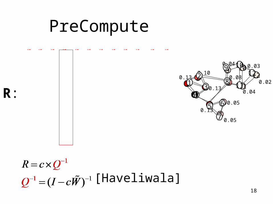
PreCompute
1 2 3 4 5 6 7 8 9 10 11 12r r r r r r r r r r r r
1
43
2
5 6
7
9 10
8 11
120.130.10
0.13
0.130.05
0.05
0.08
0.04
0.02
0.04
0.03
13
2
5 6
7
9 10
811
12
[Haveliwala]
R:

19
2.20 1.28 1.43 1.29 0.68 0.56 0.56 0.63 0.44 0.35 0.39 0.34
1.28 2.02 1.28 0.96 0.64 0.53 0.53 0.85 0.60 0.48 0.53 0.45
1.43 1.28 2.20 1.29 0.68 0.56 0.56 0.63 0.44 0.35 0.39 0.33
1.29 0.96 1.29 2.06 0.95 0.78 0.78 0.61 0.43 0.34 0.38 0.32
0.91 0.86 0.91 1.27 2.41 1.97 1.97 1.05 0.73 0.58 0.66 0.56
0.37 0.35 0.37 0.52 0.98 2.06 1.37 0.43 0.30 0.24 0.27 0.22
0.37 0.35 0.37 0.52 0.98 1.37 2.06 0.43 0.30 0.24 0.27 0.22
0.84 1.14 0.84 0.82 1.05 0.86 0.86 2.13 1.49 1.19 1.33 1.13
0.29 0.40 0.29 0.28 0.36 0.30 0.30 0.74 1.78 1.00 0.76 0.79
0.35 0.48 0.35 0.34 0.44 0.36 0.36 0.89 1.50 2.45 1.54 1.80
0.39 0.53 0.39 0.38 0.49 0.40 0.40 1.00 1.14 1.54 2.28 1.72
0.22 0.30 0.22 0.21 0.28 0.22 0.22 0.56 0.79 1.20 1.14 2.05
PreCompute:
1
43
2
5 6
7
9 10
8 11
120.130.10
0.13
0.130.05
0.05
0.08
0.04
0.02
0.04
0.03
1
43
2
5 6
7
9 10
811
12
Fast on-line response
Heavy pre-computation/storage costO(n ) O(n )
0.13
0.10
0.13
0.22
0.13
0.05
0.05
0.08
0.04
0.03
0.04
0.02
3 2

20
Q: How to Balance?
On-line Off-line

21
Roadmap
• Background– RWR: Definitions– RWR: Algorithms
• Basic Idea• FastRWR
– Pre-Compute Stage– On-Line Stage
• Experimental Results• Conclusion
22
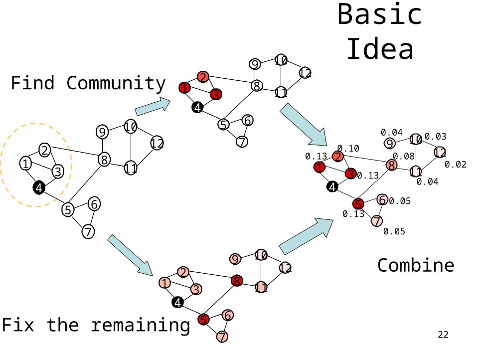
Basic Idea
1
43
2
5 6
7
9 10
8 11
120.130.10
0.13
0.130.05
0.05
0.08
0.04
0.02
0.04
0.03
1
43
2
5 6
7
9 10
811
12
Find Community
Fix the remaining
Combine1
43
2
5 6
7
9 10
8 11
12
1
43
2
5 6
7
9 10
8 11
12
5 6
7
9 10
811
12
1
43
2
5 6
7
9 10
8 11
12
1
43
2
5 6
7
9 10
8 11
12
1
43
2

23
Pre-computational stage
• Q: • A: A few small, instead of ONE BIG, matrices inversions
Efficiently compute and store Q-1

24
• Q: Efficiently recover one column of Q• A: A few, instead of MANY, matrix-vector multiplication
On-Line Query Stage
+
0
0
0
0
0
0
1
0
0
0
0
0
-1
ie ir

25
Roadmap
• Background– RWR: Definitions– RWR: Algorithms
• Basic Idea• FastRWR
– Pre-Compute Stage– On-Line Stage
• Experimental Results• Conclusion

26
Pre-compute Stage
• p1: B_Lin Decomposition– P1.1 partition– P1.2 low-rank approximation
• p2: Q matrices– P2.1 computing (for each partition)– P2.2 computing (for concept space)
11Q

27
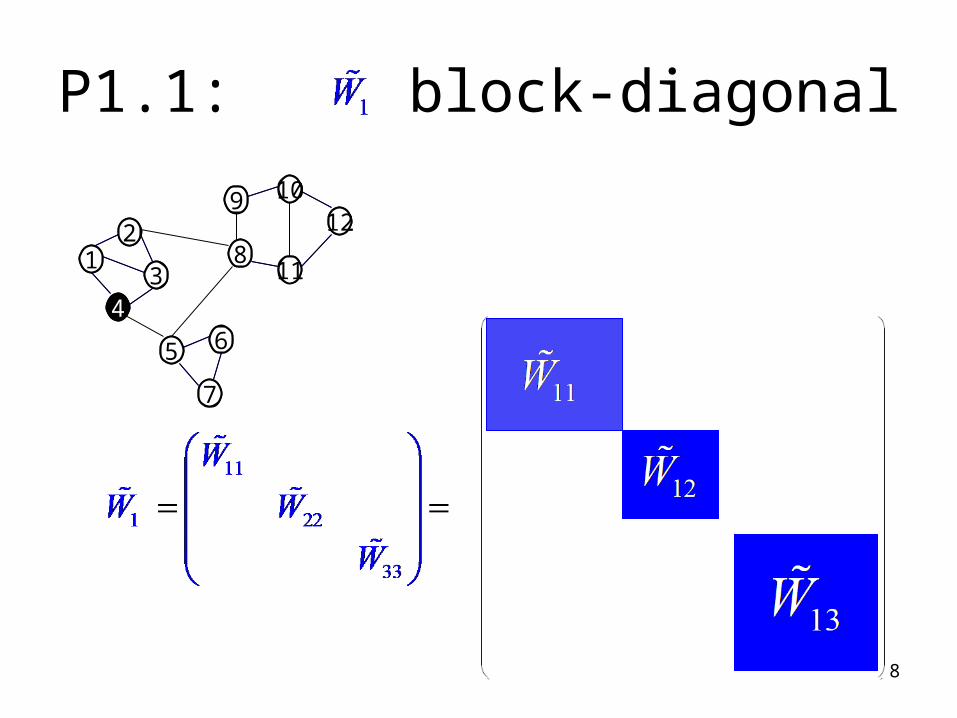
P1.1: partition
1
43
2
5 6
7
9 10
811
12
1
43
2
5 6
7
9 10
811
12
Within-partition links cross-partition links
28
P1.1: block-diagonal
1
43
2
5 6
7
9 10
811
12
1
43
2
5 6
7
9 10
811
12

29
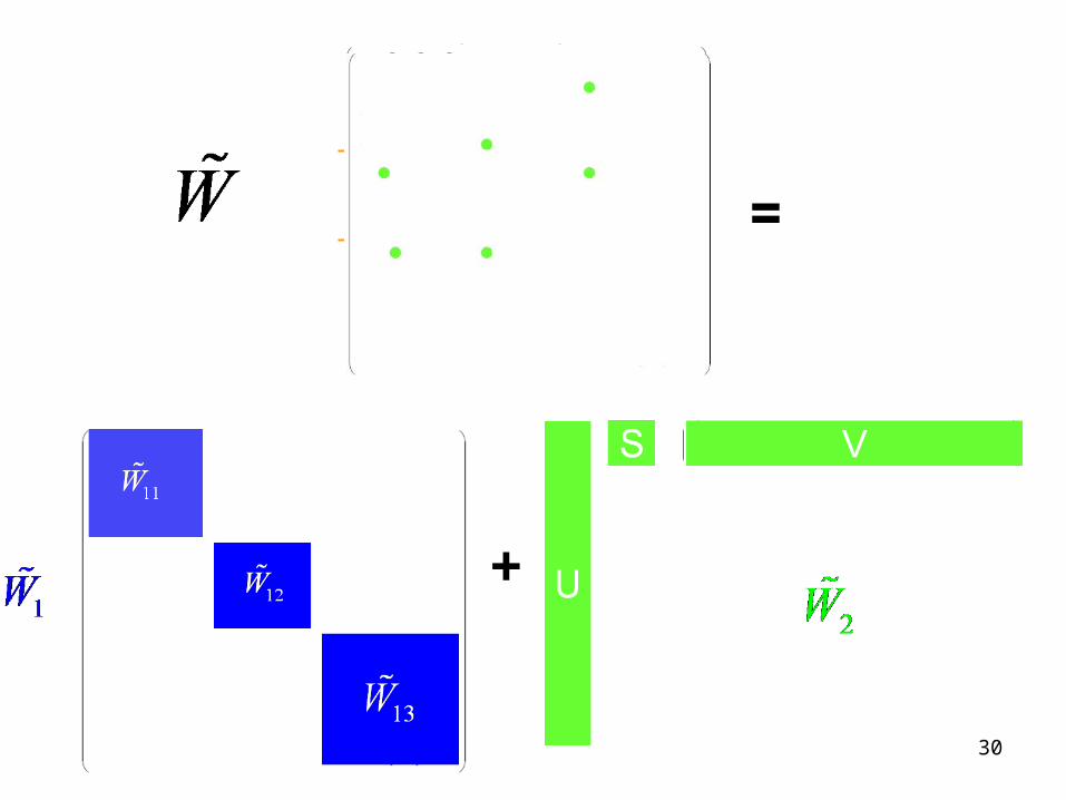
P1.2: LRA for
31
4
2
5 6
7
9 10
811
12
1
43
2
5 6
7
9 10
811
12
|S| << |W2|~
30
+
=

31
p2.1 Computing

32
Comparing and
• Computing Time– 100,000 nodes; 100 partitions– Computing 100,00x is Faster!
• Storage Cost – 100x saving!
Q 1,1
Q 1,2
Q 1,k
11Q
=
11Q
11Q
33
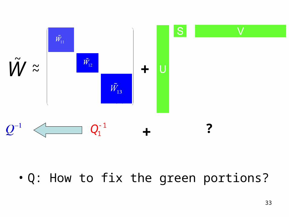
• Q: How to fix the green portions?
W +~
~~
11Q
+ ?

34
p2.2 Computing:
1S UV=_
-1
1
43
2
5 6
7
9 10
811
12
Q 1,1
Q 1,2
Q 1,k

35
SM Lemma says:
We have:
Communities Bridges
1 1 11 1
11U VcQQ Q Q
36
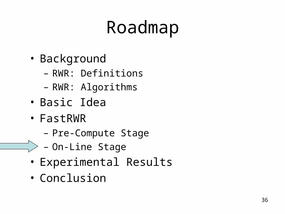
Roadmap
• Background– RWR: Definitions– RWR: Algorithms
• Basic Idea• FastRWR
– Pre-Compute Stage– On-Line Stage
• Experimental Results• Conclusion

37
On-Line Stage
• Q
+
Query
0
0
0
0
0
0
1
0
0
0
0
0
Result
?
• A (SM lemma)
Pre-Computation
ie ir

38
On-Line Query Stage
q1:q2:q3:q4:q5:q6:

39

40
Roadmap
• Background– RWR: Definitions– RWR: Algorithms
• Basic Idea• FastRWR
– Pre-Compute Stage– On-Line Stage
• Experimental Results• Conclusion
41
Experimental Setup
• Dataset– DBLP/authorship– Author-Paper– 315k nodes– 1,800k edges
• Approx. Quality: Relative Accuracy
• Application: Center-Piece Subgraph
42
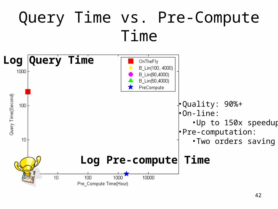
Query Time vs. Pre-Compute Time
Log Query Time
Log Pre-compute Time
•Quality: 90%+ •On-line:
•Up to 150x speedup•Pre-computation:
•Two orders saving

43
Query Time vs. Pre-Storage
Log Query Time
Log Storage
•Quality: 90%+ •On-line:
•Up to 150x speedup•Pre-storage:
•Three orders saving
44
Roadmap
• Background– RWR: Definitions– RWR: Algorithms
• Basic Idea• FastRWR
– Pre-Compute Stage– On-Line Stage
• Experimental Results• Conclusion

45
Conclusion
• FastRWR– Reasonable quality preservation (90%+)– 150x speed-up: query time– Orders of magnitude saving: pre-compute & storage
• More in the paper– The variant of FastRWR and theoretic justification– Implementation details
• normalization, low-rank approximation, sparse
– More experiments• Other datasets, other applications

46
Q&A
Thank you!
www.cs.cmu.edu/~htong