Fast Ions and Shear Alfvén Waves - UCI Physics and Astronomy

UNIVERSITY OF CALIFORNIA, IRVINE

Fast Ions and Shear Alfvén Waves

DISSERTATION

submitted in partial satisfaction of the requirements for the degree of

DOCTOR OF PHILOSOPHY

in Physics

By

Yang Zhang

Dissertation Committee: Professor William W. Heidbrink, Co-chair

Professor Roger McWilliams, Co-chair Professor Zhihong Lin

2008

ii

The dissertation of Yang Zhang is approved and is acceptable in quality and form for publication on microfilm

________________________

________________________

________________________

Committee Chair

University of California, Irvine 2008

iii

DEDICATION

To my wife Lily, and my parents,

for their love and support.

The LORD is my rock, and my fortress, and my deliverer; my God, my strength, in whom I will trust; my buckler, and the horn of my salvation, and my high tower.

Psalm 18:2

iv

TABLE OF CONTENTS

CONTENTS ………………………………………………………………………………….Page

TABLE OF CONTENTS ......................................................................................................... iv

LIST OF FIGURES .................................................................................................................vi

LIST OF TABLES.................................................................................................................... ix

LIST OF SYMBOLS................................................................................................................. x

ACKNOWLEDGMENTS......................................................................................................xiii

CURRICULUM VITAE ......................................................................................................... xv

ABSTRACT OF THE DISSERTATION.............................................................................. xvii

CHAPTER 1 INTRODUCTION...............................................................................................1

1.1 FAST IONS AND ALFVÉN WAVES IN PLASMAS .................................................................. 1 1.2 FAST-ION TRANSPORT PROJECT AT UC IRVINE ................................................................. 3 1.3 PREVIOUS CLASSICAL FAST-ION TRANSPORT STUDY ....................................................... 4 1.4 SHEAR ALFVÉN WAVES IN THE UPGRADED LAPD........................................................... 6 1.5 CONTENT OF THESIS....................................................................................................... 8

CHAPTER 2 EXPERIMENTAL APPARATUSES ................................................................12

2.1 BASIC PLASMA SCIENCE FACILITY AT UCLA—THE UPGRADED LAPD...........................12 2.2 IRVINE ELECTRON-POSITRON CHAMBER........................................................................17 2.3 IRVINE FAST-ION SOURCES.............................................................................................20

2.3.1 Thermionic Lithium Aluminosilicate Ion Sources .....................................................22 2.3.2 3-cm RF Ion Source Modification............................................................................47

2.4 SHEAR ALFVÉN WAVES ANTENNAS................................................................................48 2.5 DIAGNOSTIC TOOLS.......................................................................................................49

2.5.1 Collimated/Gridded Fast-ion Analyzers...................................................................50 2.5.2 B-dot Probes for Wave Magnetic Field ....................................................................59

CHAPTER 3 FAST-ION DOPPLER SHIFTED CYCLOTRON RESONANCE WITH SHEAR ALFVÉN WAVES .....................................................................................................62

3.1 RESONANCE THEORY.....................................................................................................63 3.2 SAW DISPERSION RELATION..........................................................................................65 3.3 RESONANCE ORBIT SIMULATION CODE..........................................................................66

3.3.1 Single particle simulation........................................................................................66 3.3.2 Monte-Carlo simulation ..........................................................................................72

3.4 RESONANCE EXPERIMENTAL SETUP...............................................................................76 3.4.1 Overview.................................................................................................................76 3.4.2 Fast-ion Signal Detection........................................................................................78 3.4.3 SAWs Launched by Loop Antenna............................................................................84 3.4.4 SAW Perpendicular Pattern.....................................................................................88

3.5 RESONANCE EXPERIMENT RESULTS...............................................................................89 3.5.1 Fast-ion Signal Shows SAW-Induced Transport .......................................................89 3.5.2 Measured Doppler Resonance Spectra ....................................................................93 3.5.3 Energy Test of Fast Ion Doppler Resonance...........................................................100

CHAPTER 4 SPECTRAL GAP OF SHEAR ALFVÉN WAVES IN A PERIODIC AR RAY

v

OF MAGNETIC MIRRORS ................................................................................................ 104

4.1 MOTIVATION ................................................................................................................105 4.2 SPECTRAL GAP ANALYTICAL THEORY..........................................................................107 4.3 SAW SPECTRAL GAP EXPERIMENTAL SETUP................................................................110

4.3.1 Mirror Array in the LAPD.....................................................................................110 4.3.2 Launching SAWs in the Magnetic Mirror Array .....................................................115

4.4 SAW SPECTRAL GAP EXPERIMENTAL RESULTS............................................................117 4.4.1 Characteristics of Wave Spectra ............................................................................117 4.4.2 Dependence of SAW Spectra on the Number of Mirror Cells..................................118 4.4.3 Characteristics of Spectral Gap and Continua.......................................................119 4.4.4 Varying Mirror Depth (M) .....................................................................................122 4.4.5 Verification: Interference Causes Spectral Gap......................................................126 4.4.6 Continuum Quality Factor Varying with Density....................................................129

4.5 SAW SPECTRAL GAP SIMULATION ...............................................................................131 4.5.1 Electro-Magnetic Wave Solver...............................................................................131 4.5.2 Periodic Array of Mirrors......................................................................................132 4.5.3 Simulation of Mirror Array in the LAPD................................................................135

CHAPTER 5 CONCLUSIONS ............................................................................................. 143

5.1 SUMMARY ...................................................................................................................143 5.2 IMPLICATIONS..............................................................................................................145 5.3 FUTURE WORK.............................................................................................................146

APPENDIX A: Typical Ion Beam and the LAPD Plasma Parameters............................. 151

APPENDIX B: Important Data Sets Supporting Experimental Results .......................... 153

APPENDIX C: Schematics for Experimental Apparatuses .............................................. 157

APPENDIX D: Instrument Calibration Data ................................................................... 164

vi

LIST OF FIGURES FIGURES ………………………………………………………………………………….Page FIG. 1.1. ILLUSTRATIONS OF WAVE-PARTICLE INTERACTIONS IN FUSION DEVICES

AND SPACE PLASMAS. ...................................................................................................2 FIG. 2.1. A PHOTOGRAPH OF THE LAPD MACHINE AND THE EXPERIMENTER........... 14 FIG. 2.2 DIAGRAM OF THE UPGRADED LARGE PLASMA DEVICE (THE LAPD) WITH

PORT NUMBERS LABELED. PORT 7, 13, 35, 41 AND 47 ARE CURRENTLY INSTALLED WITH A TOP RECTANGULAR PORT LARGE ENOUGH FOR FAST-ION SOURCES AND SAW ANTENNAS INSTALLATION. PORT 35 HAS A SIDE-ACCESS RECTANGULAR PORT IN ADDITION........................................................................... 15

FIG. 2.3. ELECTRON-POSITRON CHAMBER OF UC IRVINE ............................................. 19 FIG. 2.4. SCHEMATICS AND PHOTOGRAPHS OF LITHIUM ION SOURCES FROM HEAT

WAVE INC........................................................................................................................ 23 FIG. 2.5. CROSS SECTIONAL VIEW OF A GENERIC LITHIUM ION SOURCE IN THE

LAPD PLASMA AT A PITCH ANGLE OF 30˚. ................................................................ 25 FIG. 2.6. BEAM DIAGNOSTICS INSTALLED IN THE ELECTRON-POSITRON CHAMBER.

.......................................................................................................................................... 27 FIG. 2.7. PHOTOGRAPH VIEWING FROM ELECTRON-POSITRON CHAMBER END PORT.

.......................................................................................................................................... 27 FIG. 2.8. 0.6” EMITTER GUN EMISSION AND COLLECTION CURRENT VERSUS

ACCELERATION GAP VOLTAGE. ................................................................................. 29 FIG. 2.9. EMITTED BEAM PROFILES OF LITHIUM SOURCES.......................................... 30 FIG. 2.10. ELECTROSTATIC POTENTIAL LINES CALCULATED ACCORDING TO

DIFFERENT GUN CONFIGURATIONS..........................................................................33 FIG. 2.11. ENERGY DISTRIBUTIONS FROM 0.25” EMITTER GUN WITH DIFFERENT

EMITTER BIASES. .......................................................................................................... 35 FIG. 2.12. FAST-ION EXPERIMENTAL CONFIGURATION IN THE LAPD PLASMA

(SCHEMATIC). FIGURE SHOWS THAT FAST ION COMPLETES THREE CYCLOTRON ORBITS BEFORE BEING COLLECTED BY THE FAST-ION ANALYZER THREE PORTS AWAY FROM THE SOURCE (0.96 M). THE ANALYZER SCANS IN X-Y PLANE FOR BEAM SPATIAL PROFILE. ................................................................ 37

FIG. 2.13. EXPERIMENT FOR LITHIUM-7 ISOTOPE PURITY............................................. 40 FIG. 2.14. ILLUSTRATION OF THE MINI-LIGUN AND THE TOF DIAGNOSTIC............... 42 FIG. 2.15. INDIVIDUAL PULSES FROM LITHIUM ION SOURCE....................................... 43 FIG. 2.16. LITHIUM ION ENERGY SCAN.............................................................................. 44 FIG. 2.17. LITHIUM ION DISTRIBUTION FUNCTION. ........................................................ 46 FIG. 2.18. MATCHING EFFICIENCY CURVE OF THE MODIFIED CONNECTION OF THE

RF SOURCE. .................................................................................................................... 48 FIG. 2.19. PHOTOGRAPH OF THE LOOP ANTENNA. (T. CARTER, B. BRUGMAN, UCLA)

.......................................................................................................................................... 49 FIG. 2.20. ILLUSTRATION OF THE FAST-ION ANALYZER THAT DISTINGUISHES

FAST-ION SIGNALS FROM THERMAL PARTICLES. ................................................... 51 FIG. 2.21. TYPICAL FAST-ION ANALYZER COLLECTED SIGNAL WITH REFERENCE TO

LAPD PLASMA DENSITY AND LITHIUM SOURCE PROPERTIES (0.6” EMITTER GUN). ............................................................................................................................... 54

FIG. 2.22. CONTOURS OF 0.6” EMITTER GUN BEAM PROFILE IN THE LAPD PLASMA (COLOR BARS IN ΜA; ORIGIN AT LAPD MACHINE CENTER). ................................ 56

FIG. 2.23. WEIGHTED AVERAGE RADIAL BEAM PROFILE IN THE DISCHARGE AND THE AFTERGLOW. ......................................................................................................... 58

vii

FIG. 2.24. AN EXAMPLE OF THE ORTHOGONAL COILS IN A B-DOT PROBE.................. 59 FIG. 3.1 SINGLE-PARTICLE SIMULATION RESULTS..................................................... 68 FIG.3.2. SINGLE-PARTICLE SIMULATION RESULTS, CONT.............................................. 70 FIG.3.3 MONTE-CARLO SIMULATION FLOW CHART ....................................................... 74 FIG.3.4. MONTE-CARLO MODEL SIMULATED FAST-ION BEAM PROFILES WITH

DIFFERENT SAW PERTURBATIONS............................................................................. 76 FIG.3.5. EXPERIMENTAL SETUP AT THE LAPD.................................................................. 77 FIG.3.6 ELECTRICAL CONFIGURATIONS AND SHIELDING SOLUTIONS FOR FAST-ION

GENERATION AND DIAGNOSTICS. ............................................................................. 80 FIG.3.7. A TYPICAL LITHIUM FAST-ION BEAM PROFILE DURING THE DISCHARGE OF

THE LAPD PLASMA, WITH SUPERIMPOSED CURVES TO AID FURTHER ANALYSIS. ...................................................................................................................... 83

FIG.3.8. ARRANGEMENT OF FAST-ION SOURCE (RED DASHED) AND THE SAW FIELDS ON A PERPENDICULAR PLANE...................................................................... 86

FIG.3.9. SPECTRA OF Bx AND LOOP ANTENNA CURRENT BY TRIANGULAR DRIVE.

.......................................................................................................................................... 87 FIG.3.10. PERPENDICULAR SAW MAGNETIC FIELD PATTERNS. .................................... 88 FIG.3.11. TYPICAL FAST-ION SIGNAL TIME TRACES INFLUENCED BY SAWS AT THE

DOPPLER RESONANCE FREQUENCY.......................................................................... 91 FIG.3.12. COMPARISON OF FAST-ION BEAM PROFILE WITH AND WITHOUT SAW

INFLUENCE..................................................................................................................... 92 FIG.3.13. A) FAST-ION BEAM RADIAL PROFILES WITH VARIOUS SAW FREQUENCIES

(COLORED LINES/SYMBOLS) COMPARED TO THE UNPERTURBED PROFILE (BLACK-SOLID); B) CHANGES IN FWHM OF BEAM RADIAL PROFILES VERSUS SAW FREQUENCY; C) CHANGES IN GAUSSIAN PEAK INTENSITY (P0) VERSUS SAW FREQUENCY. (DATA ACQUIRED WITH 25 MHZ SAMPLING RATE, AVERAGING 8 SAMPLES AND 8 CONSECUTIVE PLASMA SHOTS, DEC. 07 LAPD RUN). 95

FIG.3.14. ILLUSTRATION OF WIDENED BEAM SPOT CAUSED BY BEAM

DISPLACEMENT ALONG THE r DIRECTION........................................................... 97 FIG.3.15. DOPPLER RESONANCE SPECTRA: EXPERIMENTAL AND THEORETICAL. ... 98

FIG.3.16. TYPICAL FFTS OF Bx SIGNAL LAUNCHED BY THE TRIANGULAR WAVE

ANTENNA DRIVE. ........................................................................................................ 100 FIG. 3.17. FAST-ION ENERGY CHANGE VERSUS ω AT RESONANT FREQUENCY

(SIMULATION).............................................................................................................. 101 FIG. 3.18 FAST-ION SIGNAL DETECTED WITH COLLECTOR AT HIGH BIAS (+ 480 V).102 FIG. 4.1. ILLUSTRATION OF COUPLED SHEAR ALFVÉN WAVE IN AN INFINITE

MAGNETIC MIRROR ARRAY CONFIGURATION. ..................................................... 110 FIG. 4.2. SIDE VIEW OF THE BASELINE MIRROR ARRAY CONFIGURATION (M = 0.25)

AT LAPD (LOWER HALF OF THE CHAMBER IS SEMI-TRANSPARENT)................ 112 FIG. 4.3. RADIAL PROFILES OF PLASMA PROPERTIES................................................... 114

FIG. 4.4. θB~

RADIAL PROFILES AT ∆Z = 10.24 M (PORT 14). ......................................... 116

FIG. 4.5. SAW SPECTRA WITH VARIOUS NUMBERS OF MIRROR CELLS IN LAPD. .... 119 FIG. 4.6. TWO DIFFERENT REPRESENTATIONS OF THE SAW SPECTRUM AT PORT 14

WITH THE BASELINE MIRROR CONFIGURATION (M = 0.25)................................. 121 FIG. 4.7. FOUR MAGNETIC MIRROR ARRAY CONFIGURATIONS WITH GRADUALLY

INCREASED MIRROR DEPTH..................................................................................... 123 FIG. 4.8. SAW SPECTRA FOR FOUR MAGNETIC MIRROR ARRAY CONFIGURATIONS

WITH DIFFERENT MIRROR DEPTH (M) AT PORT 14................................................ 124

viii

FIG. 4.9. DEPENDENCE OF SPECTRAL GAP WIDTH ON MIRROR DEPTH (M).............. 125 FIG. 4.10. TIME HISTORY OF THE RUNNING CROSS-COVARIANCE BETWEEN THE

WAVE FIELD AND THE ANTENNA CURRENT WITH THE BASELINE MIRROR ARRAY CONFIGURATION (M = 0.25) AT PORT 14..................................................... 128

FIG. 4.11. UPPER CONTINUUM SPECTRA WIDTH ( ++ f/γ ) WITH THREE DIFFERENT PLASMA DENSITIES. ................................................................................................... 130

FIG. 4.12. A): SIMULATION OF WAVE EXCITATION AS A FUNCTION OF sϕ AND

FREQUENCY. A SHARP FORBIDDEN GAP OF WAVE EXCITATION IS EVIDENT BETWEEN TWO BRANCHES OF TRAVELING WAVES. HERE THE WAVE AMPLITUDE IS NORMALIZED BY THE ANTENNA CURRENT. B): THE DISPERSION RELATION OF EXCITED WAVES FROM THE SIMULATION, IN WHICH F CORRESPONDS TO THE MAXIMUM OF EACH PEAK AND zsz Lk /ϕ≡ ................ 134

FIG. 4.13. COMPUTATIONAL SETUP USED TO SIMULATE THE MIRROR ARRAY IN THE LAPD SHOWN IN FIG. 4.2............................................................................................. 135

FIG. 4.14. THE RADIAL PROFILES OF AZIMUTHAL B FIELD (RMS) AT THREE FREQUENCIES COMPARING SIMULATION AND EXPERIMENTAL RESULTS. ..... 136

FIG. 4.15. COMPARISON OF θB : EXPERIMENT VERSUS THE SIMULATION............... 138

FIG. 4.16. THE CONTOUR PLOTS OF WAVE ENERGY DENSITY OBTAINED FROM EQ. (4.21) FOR THREE FREQUENCIES. ............................................................................. 140

FIG. 5.1. FAST ION TRANSPORT UNDER TURBULENCE FIELDS EXPERIMENT IN THE LAPD PLASMA. ............................................................................................................ 148

FIG. 5.2. MAGNETIC FIELD WITH DEFECT IN THE MIRROR ARRAY IN THE LAPD.... 149 FIG. 0.1 PHOTOGRAPH (LEFT) AND INSIDE STRUCTURE (RIGHT) OF THE 0.6”

EMITTER LITHIUM SOURCE (LIGUN)....................................................................... 157 FIG. 0.2. DIMENSIONS FOR ORIGINAL INNER STRUCTURES OF 0.6” EMITTER

LITHIUM SOURCE........................................................................................................ 158 FIG. 0.3. MODIFIED GRID STRUCTURE OF 0.6” EMITTER LITHIUM SOURCE SHOWING

28º OF INCIDENT ANGLE TO THE EDGE OF THE EMITTER, WITH 0.5 CM DIAMETER APERTURE................................................................................................ 159

ix

LIST OF TABLES TABLES……………………………………………………………………………………….Page TABLE 1. OVERVIEW OF FAST-ION SOURCES EMPLOYED BY THE UC IRVINE

FAST-ION GROUP IN COMPARISON WITH THE IDEAL SOURCE............................. 21 TABLE 2 LIST OF PARAMETERS FOR TYPICAL CASES OF FAST ION AND SAW

RESONANCE................................................................................................................... 72 TABLE 3 COMPARISON OF TIME RATES FOR DIFFERENT TRANSPORT MECHANISMS.

B0 = 1.2 KG....................................................................................................................... 73 TABLE 4 SIMILARITIES BETWEEN TAE AND MIRROR ARRAY ALFVÉN EXPERIMENT.

........................................................................................................................................ 145

x

LIST OF SYMBOLS

B0 Ambient Magnetic Field

Bθ Wave Magnetic Field Azimuthal Component

B Wave Magnetic Field

b Gauss Fit Coefficient Of Fast Ion Profile (Proportional To FWHM)

c Speed Of Light

cs Ion Sound Speed

e Electronic Charge

D Electric Displacement Vector

E Plasma Wave Electric Field

Ey Plasma Wave Electric Field Along The Y Direction

Ez Plasma Wave Electric Field Component Parallel To B0

/ /E Plasma Wave Electric Field Component Parallel To B0

⊥E Plasma Wave Electric Field Component Perpendicular To B0

fBragg Bragg Frequency Of A Periodic System

fG Saw Gap Frequency

f+ Saw Upper Continuum Frequency

f- Saw Lower Continuum Frequency

fci Plasma Ion Cyclotron Frequency

Iant Antenna Current

ja Antenna Current Density

k Boltzmann’s Constant

kBragg Bragg Wave Vector

k//, kz Wave Vector Component Parallel To B0

k Wave Vector Component Perpendicular To B0

La Antenna Length (Rod)

Lm Magnetic Mirror Length Perpendicular To B0

m Mass; Wave Mode Number

M Magnetic Mirror Depth

em Mass Of Electron

fm Mass Of Fast Ion

im Mass Of Plasma Ion

n Integer Wave Mode Number

xi

en Electron Density

in Plasma Ion Density

P Fast Ion Signal Intensity

qf Fast Ion Charge

r0 Gyro-Radius

r Radial Coordinate

rSAW Saw Perturbed Fast Ion Radial Coordinate

t Time

eT Electron Temperature

iT Ion Temperature

U Saw Magnetic Disk Energy Density

V Voltage

v Fast Ion Velocity

v⊥ Velocity Component Perpendicular To Magnetic Field

v, vz Velocity Component Parallel To Magnetic Field

ve Electron Velocity

vi Plasma Ion Velocity; Ion Sound Speed

fV Plasma Floating Potential

W Beam Energy

W⊥ Beam Energy Perpendicular To B0

/ /W Beam Energy Parallel To B0

x Fast Ion Coordinate

z Axial Position In The Lapd Parallel To B0

δz Fast Ion Travel Distance Parallel To B0

eβ Electron Beta To Determine Kinetic (>>1) Or Inertial (<<1) Alfvén Wave

δs Electron Skin Depth

δB Wave Magnetic Field Instensity

∆r SAW Induced Fast Ion Displacement Along The Radial Direction

∆Φ SAW Induced Fast Ion Displacement Along The Gyro Direction

0ε Permittivity Of Free Space

αβε Plasma Dielectric Tensor

θ Fast Ion Pitch Angle

eiν Electron-Ion Coulomb Collision Rate

e Landauν−

Effective Landau Damping Collision Frequency

xii

ωci Plasma Ion Cyclotron Frequency

ωpi Ion Plasma Frequency

ω Normalized Wave Angular Frequency

ρ 0 Fast Ion Beam Charge Density ρ Gyro-Radius

ρ s Ion Sound Gyro-Radius

Cyclotronτ Fast Ion Gyro Period

PASτ Pitch Angle Scattering Time

SAWτ Saw Period

trapτ Trapping Period Of Fast Ion In Wave Field

Wτ Fast Ion Slowing-Down Time

φ Gyro Phase

φ0 Phase Difference Between Fast Ion And Alfvén Wave

χ2 Chi Square Test µ Magnetic Moment

µ 0 Permeability Of Free Space

fΩ Fast Ion Gyro-Frequency

xiii

ACKNOWLEDGMENTS

I was very glad when I first got into the UC Irvine fast-ion transport group. The

faculty-to-student ratio has been 3 to 1 for nearly three years after Liangji graduated. I

don’t know if this is a nation high but I surely enjoyed the affluent experimental plasma

physics from all my advisors, Professor William W. Heidbrink, Professor Roger

McWilliams and Dr. Heinrich Boehmer.

Bill has always been an energetic researcher (it may be completely uncorrelated to

address here that his concentration is on energetic particles in fusion devices). The

experiment weeks at the LAPD facility are intense. I could barely stay awake after a

whole day of setting up instruments and tuning devices when I first started four years ago.

Now my stamina has been trained to last more than 14 hours a day, 7 days straight, all

because that Bill has set himself as a good example.

Roger is an experimental physicist, a jazz musician and an automobile hobbyist. He

taught me to train and trust my own senses before using any advanced instruments, as

well as the experimental skills in his plasma laboratory. He always shows me how

confident and eloquent a physicist can truly be. I still remember the time I was first

amazed by “Take Five” when he played sax with his band at the University Club, UC

Irvine. His performance at my wedding banquet was a great gift to Lily and me.

Dr. Boehmer’s memory is always young for all the experiments that he has done. I

learned what is called German efficiency and accuracy from him. His knowledge and

experience on fast-ion sources contributes greatly in the design and application of the

lithium fast-ion sources in this thesis. He told me that he enjoys pondering on a physics

problem in the afternoon breeze with a glass of wine. The coupled-wave model in the

xiv

second experiment of this thesis, for example, was a direct outcome of this habit.

I would also like to thank the LAPD group at UCLA, including Professor Walter

Gekelman, Dr. David Leneman, and Dr. Steve Vincena, for their hospitality at the facility

and essential support to this thesis work. Their expertise in shear Alfvén waves makes the

final fast-ion-wave resonance results possible. Professor Troy Carter and Brian Brugman

provided us with their loop antenna and power supply, Patrick Pribyl designed the b-dot

probes used in this thesis work and helped a lot with our noise reduction.

I would like to thank all the people that contributed to this thesis work at UC Irvine.

Liangji Zhao was my predecessor who initiated the transport project and finished the

fast-ion classical transport study and the Monte-Carlo simulation code. Professor Boris N.

Breizman (Univ. Texas, Austin) proposed the mirror-array experiment and Guangye Chen

(Univ. Texas, Austin) used his 2D finite difference code to simulate the spectral gap

experiment. I thank Professor Liu Chen for his enlightenment in resonance and wave

theories. I thank Virgil Laul, Rung Hulme for their helps in mechanical engineering. I

thank all the “comrade” graduate students including Wayne Harris, Yadong Luo, Deyong

Liu, Zehua Guo, Erik Trask, and Tommy Roche for their support and discussions.

I thank my dear wife, Lily Wu, for always being with me through the good times and

bad times of my graduate school life.

Above all else, I want to thank Jesus Christ for being my personal savior and helper

all the time. No matter what good I want to accomplish in my life, He always gives me

another chance to try, which turned out to be so important when doing experimental

plasma physics. I have never been this confident yet respectful when I am facing

problems in research and life.

xv

CURRICULUM VITAE

Yang Zhang

FIELD OF STUDY: Experimental Plasma Physics

EDUCATION: Ph. D. in Plasma Physics, UC Irvine 03/2008 M.S. in Plasma Physics, UC Irvine 10/2004 B.S. in Applied Physics, University of Science and Technology of China (USTC) 07/2002

COLLABORATIONS: The Basic Plasma Science Facility—the Large Plasma Device (LAPD)

UCLA 07/2004-03/2008 Guangye Chen (Department of Aerospace Engineering and Engineering Mechanics),

Boris N. Breizman (Institute for Fusion Studies), University of Texas, Austin 01/2006-03/2008

The CRPP Plasma Lab at EPFL (Lausanne, Switzerland) 01/2006-03/2008 Laboratory for Low Temperature Plasmas (KAIST, Korea) 10/2006-02/2007

HONORS & AWARDS: Regents Fellowship, $10,000, UC Irvine 09/2002-06/2004

PUBLICATIONS Observation of Fast-Ion Doppler-Shifted Cyclotron Resonance with Shear Alfvén

Waves Y. Zhang, H. Boehmer, W.W. Heidbrink, R. McWilliams (UC Irvine), S. Vincena, T. Carter, D. Leneman, P. Pribyl, W. Gekelman (UCLA), Phys. Plasmas, to be submitted 2008

Fundamental Studies of Alfvén Waves and Fast Ions in the LArge Plasma Device Proceedings of 10th International Atomic Energy Agency Technical Meeting on Energetic Particles in Magnetic Confinement Systems, Max-Planck-Institut für Plasmaphysik, Garching,

xvi

Germany 10/2007 Yang Zhang,a H. Boehmer,a B.N. Breizman,b T. Carter,c Guangye Chen,b W. Gekelman,c W.W. Heidbrink,a D. Leneman,c R. McWilliams,a and S. Vincenac, P. Pribylc (aUC, Irvine; bUniversity of Texas, Austin (UT, Austin); cUniversity of California, Los Angeles (UCLA))

Spectral Gap of Shear Alfvén Waves in a Periodic Array of Magnetic Mirrors Yang Zhang, W.W. Heidbrink, H. Boehmer, R. McWilliams (UC Irvine) Guangye Chen, B. N. Breizman (UT Austin)S. Vincena, T. Carter, D. Leneman, W. Gekelman, P. Pribyl, B. Brugman (UCLA), Phys. Plasmas, 15, 012103 01/2008

Lithium Ion Sources for Investigation of Fast-ion Transport in Magnetized Plasma Y. Zhang, H. Boehmer, W. W. Heidbrink, R. McWilliams, D. Leneman, S. Vincena, Rev. Sci. Instrum. 78, 013302 01/2007

Fast-ion source and detector for investigating the interaction of turbulence with suprathermal ions in a low temperature toroidal plasma G. Plyushchev, A. Diallo, A. Fasoli, I. Furno, B. Labit, S. H. Müller, M. Podestà, and F. M. Poli (EPFL), H. Boehmer, W. W. Heidbrink, and Y. Zhang (UC Irvine) Rev. Sci. Instrum. 77, 10F503 01/2006

Fundamental Studies of Alfvén Waves and Fast Ions in the LArge Plasma Device Proceedings of 9th International Atomic Energy Agency Technical Meeting on Energetic Particles in Magnetic Confinement Systems, Hida Earth Wisdom Center, Takayama, Japan. NIFS-PROC-63, p107 2005 Yang Zhang, H. Boehmer, W.W. Heidbrink, R. McWilliams, L. Zhao, (UC Irvine); B. Brugman, , T. Carter, D. Leneman, S. Vincena (UCLA)

PRESENTATIONS:

Observation of Fast-Ion Doppler-Shifted Cyclotron Resonance with Shear Alfvén Waves (Oral Pres.) SciDAC (www.scidac.gov) Gyrokinetic Simulation of Energetic Particle Turbulent and Transport Workshop 01/2008 21st US-European Transport Taskforce Workshop, IAEA, Boulder, CO 03/2008 Y. Zhang, W.W. Heidbrink, H. Boehmer, R. McWilliams (UC Irvine) S. Vincena, T. Carter, D. Leneman, P. Pribyl, W. Gekelman (UCLA)

Magnetic Mirror Array Induced Alfvén Spectral Gaps and Continua (Seminar) Physics and Astronomy, UCLA, 05/2007 Y. Zhang, W.W. Heidbrink, H. Boehmer, R. McWilliams (UC Irvine) Guangye Chen, Boris N. Breizman (UT Austin)S. Vincena, T. Carter, D. Leneman, W. Gekelman, B. Brugman (UCLA)

Shear Alfvén Wave (SAW) Spectra in a Periodic Magnetic Mirror Array (Oral Pres.) 12th US-European Transport Taskforce Workshop, IAEA, San Diego, CA 04/2007 Y. Zhang, W.W. Heidbrink, H. Boehmer, R. McWilliams (UC Irvine) Guangye Chen, Boris N. Breizman (UT Austin)S. Vincena, T. Carter, D. Leneman, W. Gekelman, B. Brugman (UCLA)

Transport of Fast Ions in Shear Alfvén Waves (Oral Pres.) Yang Zhang, Fast-Ion Workshop at Basic Plasma Facility, UCLA, 02/2006

xvii

ABSTRACT OF THE DISSERTATION

Fast Ions and Shear Alfvén Waves

By

Yang Zhang

Doctor of Philosophy in Physics

University of California, Irvine, 2008

Professor William W. Heidbrink, Co-Chair

Professor Roger McWilliams, Co-Chair

In order to study the interaction of ions of intermediate energies with plasma

fluctuations, two plasma immersible lithium ion sources, based on solid–state thermionic

emitters (Li aluminosilicate) were developed. Compared to discharge based ion sources,

they are compact, have zero gas load, small energy dispersion, and can be operated at any

angle with respect to an ambient magnetic field of up to 4.0 kG. Beam energies range

from 400 eV to 2.0 keV with typical beam current densities in the 1 mA/cm2 range.

Because of the low ion mass, beam velocities of 100 – 300 km/s are in the range of

Alfvén speeds in typical helium plasmas in the LArge Plasma Device (LAPD).

The Doppler-shifted cyclotron resonance (ω − kzvz = Ωf) between fast ions and shear

Alfvén waves is experimentally investigated. (ω: wave frequency; kz: axial wavenumber;

vz: fast-ion axial speed; Ωf: fast-ion cyclotron frequency. ) A test particle beam of fast

ions is launched by a Li+ source in the helium plasma of the Large Plasma Device

(LAPD), with shear Alfvén waves (SAW) (amplitude δB / B up to 1%) launched by a

xviii

loop antenna. A collimated fast-ion energy analyzer measures the non-classical spreading

of the beam, which is proportional to the resonance with the wave. A resonance spectrum

is observed by launching SAWs at 0.3 – 0.8 ωci. Both the magnitude and frequency

dependence of the beam-spreading are in agreement with the theoretical prediction using

a Monte Carlo Lorentz code that launches fast ions with an initial spread in real/velocity

space and random phases relative to the wave. Measured wave magnetic field data are

used in the simulation. Measurements of fast-ion signals on selected fast-ion energies

confirm that the particles gain/lose energy from/to the wave.

A multiple magnetic mirror array is formed at the LAPD to study axial

periodicity-influenced Alfvén spectra. SAWs are launched by antennas inserted in the

LAPD plasma and diagnosed by B-dot probes at many axial locations. Alfvén wave

spectral gaps and continua are formed similar to wave propagation in other periodic

media due to the Bragg effect. The measured width of the propagation gap increases with

the modulation amplitude as predicted by the solutions to Mathieu’s equation. A 2-D

finite-difference code modeling SAW in a mirror array configuration shows similar

spectral features. Machine end-reflection conditions and damping mechanisms including

electron-ion Coulomb collision and electron Landau damping are important for

simulation.

1

C h a p t e r 1

CHAPTER 1 INTRODUCTION

1.1 Fast Ions and Alfvén Waves In Plasmas

Fast ions are ions with energies that are much larger than typical thermal energies of

plasma constituents. In laboratory experiments, fast ions are produced by neutral or ion

beam injection, by ion cyclotron or lower hybrid heating, and by fusion reactions. In

astrophysical and space plasmas, instabilities and shocks generate fast ions. Fast ions also

are found when a hot plasma merges with a colder background plasma, as when the solar

wind collides with the magnetosphere.

Alfvén waves are also pervasive in both natural and laboratory plasmas. Alfvén

waves constitute the dominant components of the electromagnetic wave spectra in the

solar-terrestrial plasma environments and, consequently, can play crucial roles in

mechanisms from solar corona heating to acceleration of charged particles in the solar

wind1, 2, aurora and the Earth’s radiation belts. Resonances between energetic particles

and Alfvén waves are also suggested as one generating mechanism for the waves.

In many toroidal laboratory devices, Alfvén waves driven unstable by fast ions are

observed with an intense fast-ion population. For example, the famous

toroidicity-induced Alfvén eigenmode3, 4 (TAE) is the most extensively studied among

numerous other modes excited by energetic particles.4, 5 Fast ions can also be expelled by

2

these Alfvén instabilities and damage vessel components in fusion experiments.6, 7

Resonant heating of fast ions by Alfvén waves well below the ion cyclotron resonance

frequency might cause ion heating in toroidal fusion devices5, 8, 9.

The interaction of fast ions with waves and instabilities is challenging to study

experimentally because of difficulties in diagnosing the fast-ion distribution function and

the wave fields accurately, in either hot fusion devices or space plasmas. Conventional

experimental approaches are limited to non-contact, line or volume averaged methods in

a tokamak, such as various spectrometers and edge scintillators/collectors for fast ions4.

The Interplanetary Scintillation (IPS) array built at the Mullard Radio Astronomy

Observatory was a representative remote diagnostics for monitoring the solar wind

activities. Expensive spacecraft measurements near the earth can cover but a fraction of

the daunting space influenced by the solar wind.

FIG. 1.1. Illustrations of wave-particle interactions in fusion devices and space plasmas. left: wave-particle interaction in a toroidal fusion device (Pinches, Ph. D. Thesis10); right: Solar and Heliospheric Observatory (SOHO) image demonstrating the influence of the solar wind on earth’s magnetosphere.

3

1.2 Fast-ion Transport Project at UC Irvine

Starting from September 2004, this thesis work continues the effort that was awarded

$326K from 8/15/2003- 8/14/2006 as DOE grant DE-FG03-03ER54720, entitled

“Fast-ion studies in the Large Plasma Device”, where the Large Plasma Device (LAPD)11

at UCLA is a national user facility for basic plasma research. In May 2006, UC Irvine

team was renewed to be funded at $100K per year for three years. Fast-ion transport

studies are carried out with three phases. Classical fast-ion transport during the afterglow

of the LAPD was investigated during Phase I (2003 – 2005, Dr. L. Zhao). Phase II is

finished during this thesis work, which concentrates on the interactions between fast-ions

and Alfvén waves. Fast-ion nonlinear heating and transport in turbulent fluctuations will

be studied during Phase III.

During this thesis work, we have developed two lithium sources that are capable of

working at large pitch angles, published an instruments paper on the lithium sources,22

developed collimated fast-ion analyzers that detect fast-ion signals during the active

discharge plasma in the LAPD, published a physics paper on spectral gaps of Alfvén

waves in a magnetic mirror array,12 submitted a physics paper on resonant interactions of

fast ions with shear Alfvén waves,13 established collaborations with research teams from

three institutions including UCLA, University of Texas, Austin (UT Austin) and the

Ecole Polytechnique Federale de Lausanne (EPFL), and presented papers at various

domestic and international conferences.

The fast-ion sources developed are the major pieces of equipments contributed by

UC Irvine. The laboratory facilities at UC Irvine provide a valuable testbed for

4

developmental activities. The Irvine Mirror and Electron-Positron Machine (EPM) have

been modified to accommodate the entire source apparatus. New probes and source

improvements are conveniently tested at UC Irvine.

As part of their 5-year renewal (2005 – 2010), the LAPD will include two

campaigns14 in their program—a fusion-related and a space-related campaign. These

campaigns are supported by personnel and equipment that is supplied by the facility.

Approximately one month of experimental runtime will be devoted to each campaign.

The fusion-related campaign is led by Professor William Heidbrink and the focus is

“energetic ion physics of relevance to fusion research.” Many experimentalists, theorists,

and modelers from various institutions including UC Irvine and UT Austin have actively

participated. This thesis work is part of this fast-ion campaign.

1.3 Previous Classical Fast-ion Transport Study

During Phase I of the fast-ion transport project (2003 – 2005, Dr. Liangji Zhao),

classical fast-ion transport during the afterglow of the LAPD is investigated. A 3-cm

diameter rf ion gun launches a pulsed, ~300 eV ribbon shaped argon ion beam parallel to

or at 15 degrees to the magnetic field in the LAPD. The parallel energy of the beam is

measured by a two-grid energy analyzer at two axial locations (z = 0.32 m and z = 6.4 m)

from the ion gun in LAPD. To measure cross-field transport, the beam is launched at 15

degrees to the magnetic field. To avoid geometrical spreading, the radial beam profile

measurements are performed at different axial locations where the ion beam is

periodically focused. The measured cross-field transport is in agreement to within 15%

with the analytical classical collision theory and the solution to the Fokker-Planck kinetic

5

equation. Collisions with neutrals have a negligible effect on the beam transport

measurement but do attenuate the beam current. The beam energy distribution

measurements are calibrated by LIF (laser induced fluorescence) measurements15

performed in the Irvine Mirror.

The slowing-down of the fast-ion beam has been measured when the ion beam source

was in the direction parallel with the uniform magnetic field in the LAPD. The ion beam

deceleration is mainly due to the Coulomb drag by the thermal electrons. The measured

energy loss time is in agreement within 10% with the standard theoretical prediction.

The cross-field diffusion was measured when the ribbon shape ion beam was

launched at 15 degrees to the magnetic field. The cross-field spreading of the beam was

observed by scanning over the different planes normal to the magnetic field. The

measured diffusion coefficient is consistent within 15% with the classical Coulomb

collision theory and the solution to the Fokker-Planck kinetic equation.

The energy diffusion was not observed in this experiment. The beam ions in the

current experiment move so fast in the parallel direction and the fast-ion travel time is so

short ( 56 10t −×∼ sec.) that the parallel velocity diffusion (energy diffusion time 2τ ∼

sec) is obscured by initial energy spreading of the ion beam (~15 eV).

The charge-exchange and elastic scattering with the neutral particles does not have

significant effects on the measurements of the fast-ion transport in this experiment, but

the beam current decreases exponentially due to the loss of the fast ions caused by the

collisions with the neutrals. The observations are consistent with the theoretical (Monte

Carlo simulation) predictions.

6

1.4 Shear Alfvén Waves in the Upgraded LAPD

The LAPD is ideal for studying SAW because its large physical size, and sufficiently

high plasma density and magnetic field, allow it to accommodate multiple Alfvén

wavelengths. Research on SAW properties in the LAPD dates back to 1994 when a pair

of theoretical16,17 and experimental18,19 papers were published on SAWs radiated from

small perpendicular scale sources in the LAPD. Subsequently, other mechanisms were

discovered to generate Alfvén waves including a variety of inserted antennas, resonance

between the LAPD cathode and the semi-transparent anode—the Alfvén Maser20, and a

dense laser-produced plasma expansion21.

Two regimes of plasma parameters for SAW propagation have been investigated for

the cylindrical LAPD plasma with uniform axial magnetic field: the Kinetic Alfvén Wave

(KAW) for plasma electrons having a Boltzmann distribution in the presence of the

Alfvén wave fields and the Inertial Alfvén Wave (IAW) for electrons responding

inertially to the wave. The KAW is more relevant to the physics of the interior regions

of tokamak plasmas and the IAW to the edge and limiter regions. A dimensionless

parameter— 2 2v / ve te Aβ ≡ is a quantitative measure of how inertial or kinetic a plasma

region is, where v 2 /te e eT m= is the thermal electron speed with Te the electron

temperature. If 1>>eβ , the region is kinetic; if 1<<eβ , then it is inertial. The standard

MHD (magnetohydrodynamic) SAW dispersion relation is

2

6

222

44422

22

2222

// )(4

1

2

1

cici

pi

ci

pi ckckckω

ω

ωω

ω

ωω

ωω

−++−

−= ⊥⊥ , (1.1)

7

which can be reduced to the following form in the limit of ⊥<< kk// ,

2 2 2 2/// v (1 ),Akω ω= − (1.2)

where ciωωω /= and k// is the component of the wave vector parallel to the background

magnetic field. The corrections to the dispersion relation for the KAW are proportional to

22sk ρ⊥ , where ⊥k is the perpendicular wave number and sρ is the ion sound

gyro-radius ciss c ωρ /= with ( ) 2/1/ ies mTc = . The IAW correction is proportional to

22ek δ⊥ , where eδ is the electron skin depth, pee c ωδ /= with

e

epe m

en

0

2

εω = as the

plasma frequency. In this experimental work, both correction factors are on the order of

0.1 and thus negligible.

An important departure from MHD is that a component of the wave electric field may

be sustained parallel to B0 due to finite electron pressure (KAW) or inertia (IAW). This

parallel electric field can lead to energization of the background electrons and thus excite

the wave, which can be done by direct application of an oscillating charge density to a

flat, circular mesh “disk antenna”26 within the plasma, or it may be excited inductively

using a “blade antenna”15, 16 which is an externally fed current with one leg within the

plasma parallel to the background field. For either excitation mechanism, there are some

general characteristics of the radiated wave field patterns which may be illustrated by

considering the disk exciter in detail. Within or close to the inertial regime, a single SAW

cone can be excited from both antennas. Assuming azimuthal symmetry, the wave

magnetic field has one dominant component θB~

as a function of r and z:16

( ) [ ]1 //

0

sinexpantI k a

B dk J k r ik za kθ

∞⊥

⊥ ⊥⊥

∝ ∫ , (1.3)

8

in which Iant is the antenna current amplitude and a is the radius of the antenna

cross-section. There are three characteristic features of the radial profiles: 1) the field is

always zero at the disk center; 2) it increases with the radial distance away from the disk

center until reaching a peak value, the radial location of which increases with axial

distance away from the exciter; 3) upon reaching the position, redge (the location of the

outer Alfvén cone), defined by

2/ 1edge eA

r z av

ω δ ω = − + , (1.4)

the wave magnetic field decreases as 1/r.

1.5 Content of Thesis

This thesis is composed based on two major experiments. The first experiment

launches test-particle fast-ion beams in the LAPD with a narrow initial distribution

function in phase space using plasma immersible fast-ion sources22, 23. The unique LAPD

provides a probe-accessible plasma that features dimensions comparable to fusion

devices, which can accommodate both large Alfvén wave lengths and fast-ion gyro orbits.

The fast-ion beam is readily detected by a collimated fast-ion analyzer. With resonance

overlap of fast ions and shear Alfvén waves, resonant beam transport in addition to the

well calibrated classical transport is analyzed with good phase-space resolution.

The second experiment studies shear Alfvén wave (SAW) propagation and forbidden

gap formation in a periodic magnetic mirror array. The experiments are performed in the

Large Plasma Device (LAPD). Although the number of mirror cells is limited, the LAPD

is capable of generating a magnetic mirror array resembling the multi-mirror magnetic

9

confinement fusion devices24 , 25 in Novosibirsk, Russia. An advantage of the

low-temperature plasma in the LAPD is its accessibility to a variety of probes. Alfvén

wave propagation and interference can be studied with spatial resolution of ~ 1 – 10 mm.

To further investigate the Alfvén spectral gaps and continua, a cold-plasma wave code26

is adapted to launch Alfvén waves in a virtual LAPD with the number of mirror cells

ranging from a few to infinite. Measured plasma parameters are used in the code to

simulate wave spectra which are compared with experimental observations.

The arrangement of this thesis is as follows. Most of the important experimental

hardware including the lithium fast-ion sources, detectors and the LAPD facility are

introduced in Chapter 2. The results of fast-ion Doppler-shifted cyclotron resonance

experiment are presented in Chapter 3 and the phenomenon of SAW spectral gaps in the

LAPD mirror array is discussed in Chapter 4. A conclusion to the Phase II of the fast-ion

transport project and future work in the coming Phase III are stated in Chapter 5.

10

1 Joseph V. Hollweg and Philip A. Isenberg, J. Geophys. Res. 107 ( A7), 1147 (2002).

2 Valentin Shevchenko, Vitaly Galinsky, and Dan Winske, Geophys. Res. Lett. 33, L23101 (2006).

3 C. Z. Cheng, L. Chen, and M. S. Chance, Ann. Phys. 161 (1985) 21.

4 W.W. Heidbrink, Phys. of Plasmas, 15, 055501 (2008)

5 King-Lap Wong, Plasma Phys. Cont. Fusion 41. R1 (1999).

6 H. H. Duong, W. W. Heidbrink, E. J. Strait, et al., Nucl. Fusion 33, 749 (1993).

7 R. B. White, E. Fredrickson, D. Darrow et al., Phys. Plasma 2, 2871 (1995).

8 L. Chen, Z. H. Lin, and R. White, Phys. Plasmas 8, 4713 (2001)

9 R. White, L. Chen, and Z. H. Lin, Phys. Plasmas 9, 1890 (2002).

10 S. D. Pinches, Ph. D. thesis, University of Nottingham, 1996,

http://www.rzg.mpg.de~sip/thesis/node1.html.

11 W. Gekelman, H. Pfister, Z. Lucky, J. Bamber, D. Leneman, and J. Maggs, Rev. Sci. Instrum. 62,

2875 (1991)

12 Yang Zhang, W.W. Heidbrink, H. Boehmer, R. McWilliams, Guangye Chen, B. N. Breizman, S.

Vincena, T. Carter, D. Leneman, W. Gekelman, P. Pribyl, B. Brugman, Phys. Plasmas, 15, 012103

(2008)

13 Yang Zhang, W.W. Heidbrink, H. Boehmer, R. McWilliams, S. Vincena, T. Carter, W. Gekelman, D.

Leneman, P. Pribyl, Phys. Plasmas, submitted, 2008

14 http://plasma.physics.ucla.edu/bapsf/pages/current.html

15 D. Zimmerman, Master thesis, University of California, Irvine (2004)

16 G. J. Morales, R. S. Loritsch, and J. E. Maggs, Phys. Plasmas 1, 3765 (1994).

17 G. J. Morales and J. E. Maggs, Phys. Plasmas 4, 4118 (1997).

18 W. Gekelman, D. Leneman, J. Maggs, and S. Vincena, Phys. Plasmas 1, 3775 (1994).

19 W. Gekelman, S. Vincena, D. Leneman, and J. Maggs, J. Geophys. Res. 102, 7225 (1997).

20 J. E. Maggs, G. J. Morales, and T. A. Carter, Phys. Plasmas 12, 013103 (2005).

11

21 M. VanZeeland, W. Gekelman, S. Vincena and G. Dimonte, Phys. Rev. Lett. 87 (10), 2673 (1999).

22 Y. Zhang, H. Boehmer, W. W. Heidbrink, R. McWilliams, D. Leneman and S. Vincena, Rev. Sci.

Instrum. 78, 013302 (2007).

23 H. Boehmer, D. Edrich, W.W. Heidbrink, R. McWilliams, and L. Zhao, Rev. Sci. Instrum., 75, 1013

(2004).

24 A. A. Ivanov, A. V. Anikeev, P. A. Bagryansky, V. N. Bocharov, P. P. Deichuli, A. N. Karpushov, V.

V. Maximov, A. A. Pod’minogin, A. 1. Rogozin, T. V. Salikova, and Yu. A. Tsidulko, Phys. Plasmas 1

(5), 1529 (1994).

25 E. P. Kruglyakov, A. V. Burdakov, and A. A. Ivanov, AIP Conf. Proc. 812, 3 (2006).

26 Guangye Chen, Alexey V. Arefiev, Roger D. Bengtson, Boris N. Breizman, Charles A. Lee, and

Laxminarayan L. Raja, Phys. Plasmas 13, 123507 (2006).

12

C h a p t e r 2

CHAPTER 2 EXPERIMENTAL APPARATUSES

For modern experimental physicists, conventional apparatuses and emerging

electronic devices are necessities for a successful experiment. Computational models on

the other hand are often regarded as theorists’ specialty tools. This thesis work requires

applications of all of the above. This chapter discusses hardware tools used in this

project:

Sec. 2.1: The upgraded LAPD, the discharge plasma;

Sec. 2.2: Irvine Electron-Positron chamber—the test bed in Irvine;

Sec. 2.3: Fast-ion sources developed at UC Irvine;

Sec. 2.4: Shear Alfvén wave antennas;

Sec. 2.5: Diagnostic tools for plasma, fast ions and Alfvén waves.

2.1 Basic Plasma Science Facility at UCLA—the Upgraded

LAPD

The Basic Plasma Science Facility at UCLA commenced in August of 2001. It is a

frontier plasma research user facility. The core of the facility is a modern, large plasma

device (the LAPD) constructed by Professor Walter Gekelman (the facility director) and

13

his staff of reserch scientists and technicians. The first plasma was achieved in July, 2001

and the machine is now in operation. Usage of the facility is available to scientists from

national and international institutions, as well as industry. The unique nature of the LAPD

enables understanding of topics on the fundamental properties of plasmas related both to

fusion energy and space science.

The cylindrical vacuum chamber of the LAPD is one meter in diameter, ~ 20 m long,

and has excellent diagnostic access. The device produces reproducible plasmas at 1 Hz

continuously. The magnetically confined, linear plasma is generated by applying a 50 –

100 V voltage pulse between a 75 cm diameter Barium Oxide cathode and a grid anode

with a ~ 2 kA discharging current pulse at a 1 Hz repetition rate. Operating gases include

hydrogen, helium, argon and neon with partial pressures controlled by individual leak

valves and monitored by a central Residual Gas Analyzer (RGA). During the discharge

of 8 - 10 ms duration, the plasma density can reach 5 x 1012 cm-3 with an electron

temperature of 10 eV. The plasma density decays in the afterglow with an initial time

constant of ~10 ms; the plasma temperature drops within ~100 µs. While the plasma

contains various modes of turbulence during the discharge, it is quiet in the afterglow.

Normally, a uniform, ~1 kG magnetic field is employed but reconfiguration of the coils

and higher field strengths are possible. Plasma parameters and fluctuations are diagnosed

with a millimeter wave interferometer (at port 23), Langmuir probes of various

configurations and three axis b-dot probes for the measurement of magnetic field

fluctuations, for example of Alfvén waves. A sophisticated data acquisition system

consisting of computer-controlled actuators, digitizers, and workstations accommodate

automated probe scans.

14

For this thesis work and the planned fast-ion investigations of plasma turbulence,

helium is the major working gas. It will primarily focus on fast-ion interactions with

waves and turbulence during the high-density discharge, when the fast-ion beam density

of 5.0 x 108 cm-3 is typically four orders of magnitude smaller than the plasma density

during the discharge.

FIG. 2.1. A photograph of the LAPD machine and the experimenter.

15

FIG. 2.2 Diagram of the upgraded LArge Plasma Device (the LAPD)* with port numbers labeled. Port 7, 13, 35, 41 and 47 are currently installed with a top rectangular port large enough for fast-ion sources and SAW antennas installation. Port 35 has a side-access rectangular port in addition.

* http://plasma.physics.ucla.edu/bapsf/pages/diag2.html

16

The LAPD has excellent access for probes and optics. There are 450 radial ports, 64

of which are rectangular quartz windows, allowing a nearly 360 degree view of the

plasma in 8 locations along the machine length1. There are sixty rotatable "ball valve"

flanges, which allow probe placement anywhere in the plasma volume between pairs of

axial field magnets. Large devices can be introduced through the rectangular ports at

seven locations using custom-built square valves.

Aside from the large size and excellent accessibility, the LAPD has other attractive

features:

Programmable confining magnetic field can be up to 3.5 kG with error less than

3%.

Three portable cryo-pump vacuum stations and numerous gate valves for

differential pumping when probes or other devices are moved in and out of the

system without breaking vacuum.

Computer controlled 2D stepping motors can move probes with 0.5 mm

accuracy throughout the plasma column.

Data acquisition system with 12 channels of 8 bit, 5 GS/s digitizers, and 32

channels of 14-bit, 100 MS/s digitizers.

Plasma density diagnostics include a 56 GHz microwave interferometer for

line-integrated density measurements and four newly-installed interferometers

located at port 15, 23, 32 and 40.

Fifteen Digital Oscilloscopes ranging from 2 channel-175 MHz/channel to 4

channel-2 GHz/channel, 6 Stanford digital delay generators (1 ps accuracy), 2

BNC 8 channel pulse generators ( 1 ns accuracy), 1 LeCroy arbitrary waveform

17

generator (10 MHz), 2 Agilent arbitrary waveform generators (80 MHz), HP

8568B spectrum analyzer, 3 LeCroy 1820A Differential Amplifiers/Filters,

Agilent Network Analyzser (to 180 MHz), 2 four channel Tektronix-Sony 100

MHz optical isolators, 2 microscopes for probe construction (one with

micro-manipulators).

2.2 Irvine Electron-Positron Chamber

The Irvine Electron-Positron chamber is located in the McWilliams Plasma

Laboratory at UC Irvine. The machine was used for electron-positron plasma study by Dr.

H. Boehmer because of its high-vacuum capability (down to 8.0 x 10-9 torr) with a Varian

Turbo-450 pump system (Model: 969-9042). A photo of a typical setup of the chamber is

shown in FIG. 2.3. Most of the developing and testing of the lithium fast-ion sources,

including the initial activation of a lithium aluminosilicate source, the beam radial-profile

and energy scan measurements, and other equipment checks for a coming LAPD run, are

conducted in the Electron-Positron chamber.

The Electron-Positron chamber has been modified to a versatile test bed of equipment.

The original chamber is about 15 cm in diameter and has three sections connected using

conflat copper o-rings for excellent vacuum sealing. The total length is about 1.2 m. A 13

cm diameter stainless steel collector and a small 0.3 cm diameter rotary probe are

mounted on top of the center section. The turbo pump inlet is connected to the bottom of

the center section with a screen in between to protect the blades in the turbo pump. A new

cross section is added to extend the original chamber. The newly developed lithium

source re-coating device is currently installed in the cross. An aluminum square spool

18

similar to the rectangular port on the LAPD is connected with the cross through a KF-50

quick-disconnect valve. This spool can accommodate either the 0.6” lithium source or the

RF source. There are two sets of water cooled magnets to provide a mirrored background

magnetic field in the vacuum chamber if necessary. The magnetic field can be up to 2.4

kG at the center of the magnets and 1.2 kG at the center section with 100 A coil current.

19

FIG. 2.3. Electron-Positron chamber of UC Irvine a) Setup of UC Irvine Electron-Positron chamber with the RF fast-ion source in the square spool and the Mini-LiGun from side KF-50 port; b) Schematics of the Electron-Positron chamber.

a)

20

2.3 Irvine Fast-ion Sources

The proposed investigations and the fact that the ion source has to be immersed in

the plasma put severe constraints on the properties of the ion gun. An ideal source for this

research should have these features (Table 1):

• Wide energy range (400 – 2000 eV) to investigate the energy dependence of the

interaction;

• Low beam ion mass to be able to match the phase velocity of Alfvén waves in

helium plasmas;

• Operation at magnetic fields up to 4 kG and at any pitch angle;

• Low beam divergence to make the beam observable over large distances;

• Small energy dispersion;

• High current density to facilitate diagnostics, but small enough to prevent

collective wave excitation (test particle investigation);

• Small gas load;

• Source operation independent of plasma conditions (density, temperature, etc.);

• Small size to minimize the perturbation of the background plasma;

• No magnetic material.

21

Table 1. Overview of fast-ion sources employed by the UC Irvine fast-ion group in

comparison with the ideal source.

22

Initially in this program, a commercial argon ion gun from IonTech, featuring a RF

discharge as the ion source, was modified for operation in the LAPD2 and used to

investigate classical transport3 and for preliminary turbulent transport measurements4

(Sec. 2.3.2). Although fairly reliable in operation, it could not be operated at pitch angles

larger than 25o and only at magnetic fields of ~ 1 kG or less. Furthermore, it has much

reduced beam production with helium compared to argon, because the higher ionization

potential prevents the formation of a sufficiently high plasma density in the source RF

coil. A new fast-ion source with features compensating the RF source is necessary, and

presumably with different mechanism in fast-ion generation.

2.3.1 Thermionic Lithium Aluminosilicate Ion Sources

Alternatives to plasmas discharges as charged particle source are the solid-state

thermionic emitters. While they are widely used as electron emitters, they are used

infrequently as ion sources because of their limited current density. Of particular interest

as a thermionic ion emitter for the fast-ion program is lithium aluminosilicate (LAS). The

type of aluminosilicate used in this article is Beta Eucryptite5,6. Apart from lithium, these

ceramics are also available for other alkali ions: sodium, potassium and cesium. Because

of their ceramic nature, these emitters are inert to atmospheric constituents at room

temperature, but deteriorate in the presence of oxygen, vacuum oil, etc. at operating

conditions (1000 – 1200º C).

LAS sources have been used before in plasma related experiments. A small gridded

23

lithium ion source was used to investigate ion drift orbits in the vacuum magnetic field of

the Compact Auburn Torsatron7. Lithium ion and neutral beam sources, placed externally

to the plasma chamber, are also used for optical and beam probe diagnostics in tokamak

and stellarator configurations(8,9,10,11,12). Since these sources are operated in the absence of

plasma electrons and system magnetic fields, they can employ a Pierce configuration13,

which generates low emittance, high current density beams.

FIG. 2.4. Schematics and photographs of lithium ion sources from Heat Wave Inc. (a) Model 101142 0.6” Dia. Ion source; (b) Model 101139 0.25” Dia. Ion source. http://www.cathode.com/i_alkali.htm

24

A. Lithium Ion Source Design And Characterization

The Pierce geometry is the ideal configuration for charged particle sources since it

has no beam perturbing grid structures. Unfortunately, it can not be used for the

investigations of fast-ion behavior in plasmas because the background plasma

constituents streaming into the gun will modify the vacuum electric field of the electrodes.

In addition, the external magnetic field will modify the beam orbits within the large

physical structure of a Pierce source. Therefore, a gridded gun configuration was chosen

in which the emitter – extraction grid separation was small enough to render beam orbit

modifications within the gun structure by 0×v B and 0×E B forces insignificant.

Two lithium ion guns with lithium aluminosilicate as thermionic emitters of different

sizes (0.6” and 0.25” diameter, Heat Wave Inc.14) were designed, constructed and

characterized at UC Irvine. Lithium emitters with typical isotope concentrations of 92.5%

Li-7 and 7.5% Li-6 are chosen for testing the fast-ion sources. Li-7 isotopically purified

emitters are used for the fast-ion transport experiments (Chapter 3). The cross section of a

generic lithium ion gun is schematically shown in FIG. 2.5. The actual configurations are

scaled to the two different emitter sizes (Appendix C). While the gun with the 0.6”

emitter is the prototype, the smaller gun was developed to decrease the perturbation of

the LAPD plasma by the gun housing and to be able to use standard 50 mm diameter

vacuum interlock valves of LAPD. Both guns were tested first in the Electron-Positron

chamber’s ultrahigh vacuum environment.

25

FIG. 2.5. Cross sectional view of a generic lithium ion source in the LAPD plasma at a pitch angle of 30˚. Shaded area corresponds to the beam extraction region, which is also the domain used to simulate the field line configuration in FIG. 2.10.

26

Since the ion emission from LAS is not purely a thermally activated process but can

be enhanced by an external electric field (Schottky effect), it is desirable to have a high

potential difference between the emitter and the first grid. Therefore, to produce

sufficient beam currents even at low beam energies, an acceleration–deceleration strategy

is employed where the emitter is biased positive (with respect to the gun housing and the

second grid) to the desired beam energy while the first grid is biased to an appropriately

high negative potential. Measured by a laser beam, the optical transparency of the

grid-system poses an upper bound for the beam transmission efficiency (collection

current/emission current). Strong field line distortions or space charge effect will cause

the beam transmission efficiency to decrease from the optical transparency.

The ion guns are first tested in the Electron-Positron chamber, usually without the

presence of a plasma to neutralize the beam space charge. The distance from emitter to

exit, respectively, is 1.88 cm for 0.6” emitter source and 1.45 cm for 0.25” emitter source.

During vacuum operations, it was observed that the collector and the probe have to be

within a few centimeters from the source exit to measure the beam current. As indicated

in FIG. 2.2 a), a collector plate, a radial rotary probe and a Faraday cup are all installed on

the top flange of the center section. The probe can be rotated manually to cross the center

of the beam for measurement, or kept away from the beam while using the collector or

the Faraday cup.

27

FIG. 2.6. Beam diagnostics installed in the Electron-Positron chamber.

To test the basic performance of the ion guns, the emission current was monitored as

a function of emitter temperature as measured by an optical pyrometer viewing the

emitter through a quartz vacuum window at one end of the Electron-Positron chamber.

The emissivity of the emitter surface, assuming ε = 0.8, could cause ~ 65 ºC of

temperature underestimate. In this work, the emitter temperature is recorded without

emissivity corrections and serves as a relative indicator of beam current performance.

FIG. 2.7. Photograph viewing from Electron-Positron chamber end port. 0.6” emitter lithium source heater on: 5.0 V, 8.4 A (left) and 5.68 V, 9.24 A (right).

28

For the 0.6” emitter at 1150 ºC and biased to 2 kV, the observed current is 2 mA

which corresponds to a current density of 1 mA/cm2. Because the 0.6” diameter beam is

more than sufficient for this fast-ion transport investigation, to achieve a better spatial

resolution, this gun is usually operated with a 5 mm diameter circular aperture. The

secondary electron emission from the 1st grid is measured to be less than 1% of emission

current, which causes less than 10% of ion transmission overestimate. With two 40 lines

per inch (lpi), 91% transmission Molybdenum grids, the optical transparency is 81%. FIG.

2.8 compares the emission current and the current to an outside collector (2.5 cm from

the emitter) as a function of extraction voltage with the emitter temperature at 1050 ºC.

The space charge limit at 1000 V of extraction voltage is ~200 µA, which indicates that

most of the current levels are limited by thermionic emission instead of space charge

effect. On average, near 80% of the ion beam is transmitted through the grid holes with

the acceleration voltage above 500 V. Positioning the gun axis at an angle of 45o with

respect to an external magnetic field of up to 4 kG did not result in a change of emission

current. FIG. 2.9 (a) shows the beam cross-section 5 cm outside the gun in the UC Irvine

chamber, using a 3 mm diameter disk collector, demonstrating good beam optics. It

should be noted that in FIG. 2.9, the emitter current was intentionally kept low at (a) ~ 0.1

mA and (b) ~ 10 µA to reduce radial space charge modification of the beam profile. In

FIG. 2.9 (b), the beam radial profile is still widened by ~ 10% from the radial

expansion.

29

FIG. 2.8. 0.6” emitter gun emission and collection current versus acceleration gap voltage. Beam transmission efficiency is calculated for each pair of current levels. (Total grid optical transparency is 81%.)

30

FIG. 2.9. Emitted beam profiles of lithium sources. (a) 0.6” emitter gun beam profile across beam center collected 5 cm away from the beam exit. Profiles are taken with +2.0 kV emitter bias and 1050˚C emitter temperature; (b) Comparison of 0.25” emitter gun beam profiles before and after modifying 1st grid structure. Profiles are taken with +600 V emitter bias, –100 V 1st grid bias and 1050˚C emitter temperature.

31

Distortion of the ion orbits within the gun structure can be caused by the fringing

fields at the edge of the emitter and the grid support rings as well as by equipotential

surface deviations from being strictly parallel in close vicinity of the grid wires. These

effects are more prevalent for the small diameter emitter. Furthermore, care must be

taken to place insulating structures in such a way that accumulated charges will not

distort the field. To visualize the electric field pattern within the actual gun structures, the

Femlab software (COMSOL, Inc.) is used to calculate the 2D equipotential lines in

cylindrical coordinates and estimate the space charge effect (FIG. 2.10 (a), (b) and (c)).

The models’ boundary conditions are set at typical operating conditions. Since Femlab

lacks a poisson solver, the space charge effect of the beam is estimated by imposing

uniformly distributed space charge along the beam path. A 0.1 mA/cm2 , Li ion beam at

600 eV energy corresponds to a reference charge density of ρ0 (7.23 x 10-6 C/m3). A

potential barrier comparable to the beam energy does not appear in the source until the

imposed charge density is increased to 100ρ0. It can be seen that for the 0.6” emitter gun

(FIG. 2.10 a) the fringing fields and the field distortions around the grid wires are

minimal. Since this ion gun is usually operated with a 0.5 cm aperture, sampling only the

center part of the beam, it produces a high quality beam. In contrast, the 0.25” emitter

gun, where, to reduce edge effects, the emitter – grid spacing was reduced from 2.50 to

1.25 mm, these effects are more severe. FIG. 2.10 b) shows the field pattern for the 0.25”

emitter gun initial design using a 40 lpi first grid. Because the grid is much closer to the

emitter, the equipotential lines are greatly distorted around the grid wires, compared to

FIG. 2.10 a) where the same grid size but a larger spacing was used. In addition, in the

deceleration stage, the fringing field in the grid support ring reaches to the center of the

32

beam. As a result of both effects, the radial beam profile for this gun is wider than the

emitter diameter (FIG. 2.9 (b)) and the transmitted beam current is greatly reduced (~

30% of emission current). To improve the beam quality, a 90 lpi first grid was installed

and an additional 40 lpi grid was installed on the opposite side of the grid support ring

with a wider aperture (0.40” I.D.). The improvement of the field pattern is evident from

FIG. 2.10 c). Although the radial distribution of the beam (FIG. 2.9 (b)) is similar, the

transmitted beam current doubles with the modified design, in spite of the total optical

transparency dropping from 81% to 64%. The beam transmission efficiency is also

improved to be ~ 49 – 66 % (uncertainty caused by possible secondary electron emission)

that is comparable to the optical transparency.

33

FIG. 2.10. Electrostatic potential lines calculated according to different gun configurations. (a) 0.6” emitter gun; (b) 0.25” emitter gun initial design with a single 1st grid next to the emitter; (c) 0.25” emitter gun modified design with two 1st grids biased negatively. Cylindrical symmetry is assumed in simulations and all grid sizes are to scale (may appear to be a single dot). Dashed boxes show where space charge is uniformly distributed along the beam paths. Simulations are powered by Femlab (COMSOL, Inc.).

34

The large diameter planar collector that measures the total emitted beam current was

used to acquire the energy distribution of the beam by taking the derivative of the

collected current with respect to the collector bias. FIG. 2.11 gives examples of the beam

energy distributions for the 0.25” emitter gun. The width is about 4% of the beam energy

without deconvolving the energy resolution of the collector15. For these LAS emitters ,

the actual energy spread of a near zero energy beam is given by a Maxwellian

distribution determined by emitter temperature, which is about 0.25 eV. The low energy

tail of the distributions, becoming more prominent with increasing beam extraction

voltage, is likely due to the field line deviations from directions perpendicular to the

emitter, e.g. those around the wires of the extraction grids, as well as increased resolution

width of the collector at higher beam energy.

From these results it is evident, that great care has to be taken in the design of

gridded guns for good performance, and that the equipotential surfaces in the acceleration

and deceleration stages of the gun should deviate from planes as little as possible since

these field errors influence both the energy spread and the divergence of the beams. Edge

effects can be minimized by extending the parallel planes defined by emitter and first grid

to larger radii. In the acceleration stage, this is accomplished by providing a shield

structure around the emitter and by the grid support ring. In the deceleration stage, again

to provide flat equipotential planes, extra grids are sometimes necessary even though they

decrease the total optical transparency.

35

FIG. 2.11. Energy distributions from 0.25” emitter gun with different emitter biases. Data taken with – 100 V 1st grid bias and 1100 ˚C emitter temperature.

With a specially fabricated power supply (Appendix C) for high voltages and heater

current, the ion guns can be operated either in the DC mode or pulsed at the 1 Hz

repetition rate of the LAPD plasma using a minimum 15 ms pulse length. From the

experience of operating the larger gun at LAPD, the emitter lifetime was found to be

about 20 hours for an average beam current density of 1 mA/cm2. In a high vacuum

environment, the lifetime is considerably longer according to Heat Wave Labs, Inc.

36

B. Operation Of Lithium Sources In The LAPD

The introduction of the lithium fast-ion sources into the LAPD machine is a time

consuming process, mainly due to the out gassing of the heater. The lithium sources are

transported to UCLA with freshly replaced emitter pre-installed. Several layers of tight

bagging are convenient to prevent excessive water vapor during transportation. Taking #

35 side rectangular port on the LAPD as an example, 0.6” emitter source is first

mechanically installed on the spool, pumped down to ~ 5 x 10-6 torr using a cryo-pump

system in about two hours. Then the source needs to be out gassed at ~ 5.0 A and

monitored by an RGA for H2O partial pressure since oxygen is a major poison for the

LAPD cathode. The H2O partial pressure will first rise up then drop down to ~ 6 x 10-6 in

another two hours before opening the gate valve. It is advisable to coordinate the whole

process with other activities for efficiency.

Supported by stainless steel tubes that also carry the heater and high voltage cables,

the ion guns are placed into the LAPD vacuum chamber at various points along the axis

of the system. Differentially pumped chevron seals allow radial motion and rotation of

the guns without vacuum leaks. The ion gun and power supply system can be separated

electrically from the vacuum chamber ground. This allows the ion gun to float at the

plasma potential, decreasing the perturbation of the plasma by the ion gun housing. The

plasma – ion gun configuration at LAPD is shown schematically in FIG. 2.12.

37

FIG. 2.12. Fast-ion experimental configuration in the LAPD plasma (schematic). Figure shows that fast ion completes three cyclotron orbits before being collected by the fast-ion analyzer three ports away from the source (0.96 m). The analyzer scans in x-y plane for beam spatial profile. Operation of these ion guns inside a plasma environment has pros and cons

compared to operation in a vacuum field chamber. In the LAPD plasma, the beam with

the maximum current output is charge neutralized by the plasma electrons since the

plasma charge density, even during the afterglow, exceeds that of the beam by three

orders of magnitude, which is an obvious benefit for the fast-ion beam orbit studies.

There are also issues to be aware of when the source is immersed in a plasma. Firstly,

since the ion sources are often floated to reduce plasma perturbation, the exiting fast-ion

energy is referenced to plasma floating potential, which is subject to change of plasma

conditions. For example the floating potential in the discharge is ~10 V higher than that

in the afterglow, which causes ~10 eV of difference in beam energy given identical

extraction grid biases. Secondly, because the emitter is at the positive beam voltage and

because the grid holes, for any useful plasma density, are large compared to the Debye

length, plasma electrons can reach the emitter electrode of the ion gun. For operation in

the afterglow phase of the LAPD plasma, this just adds a few mA to the load of the high

38

voltage power supply, but otherwise does not impair the function of the ion gun. On the

other hand, during the high-density discharge, this current becomes excessively large. In

this case, the ion gun must be positioned at a sufficiently large pitch angle so that the

plasma electrons, tied to the magnetic field lines, are prevented from reaching the emitter,

which is schematically indicated in FIG. 2.5.

C. Experimental Determination of Lithium Isotope Concentration

The natural abundance of lithium-7 is 93%, with the remaining fraction to be

lithium-6. HeatWave Labs Inc. claimed their isotopically purified lithium-7 sources reach

99.99% grade of purity. To be objective about this number, a separate experiment was

conducted to determine the bottom line of the lithium-7 purity in a commercial 0.6” Dia.

lithium-7 source—using the LAPD as a large mass-spectrometer chamber (data set

indicated in Appendix B).

The plasma-fast-ion parameters are based on the Doppler resonance case (III) used in

Chapter 2. At first, a theoretical calculation predicts a ~ 90º difference in the collected

gyro phase between the Li-7 peak and Li-6 peak. The typical beam spread along the gyro

direction is ~ 40º, which means a weak Li-6 peak would has negligible effect on the main

Li-7 spot. Then in the experiment, a Li-7 spot is scanned with B0 = 1200 G, followed by

another scan with B0 changed to 1110 G, which would move the Li-6 spot, if any, to the

center of the same grid. The lithium source is pulsed on for ~ 20 ms with a initial rising

time of ~10 ms and a eventual decaying time of > 50 ms.

The data with the flat-energy duration (FIG. 2.13 b) of the lithium source pulse shows

39

> 91% purity. Averaged fast-ion net signal over the flat-energy time slot and the area of

the beam spot is calculated for 1200 G and 1110 G data. The 1200 G data show a strong

Li-7 spot as expected with the correct energy; the 1110 G data has a strong influence from

the Li-7 spot with lower beam energies (~ 575 eV) but a weak Li-6 spot does show up

towards the end of the flat-energy duration.

The slow decaying duration of the emitter bias is very useful for calibrating the

fast-ion energy, as shown in FIG. 2.13 a). Fast-ions traveled different numbers of

gyro-cycles with different initial energies at the collection plane, which corresponds to

multiple peaks shown in a). The energies of the peaks and the theoretical gyro-cycles

match in FIG. 2.13 c), which facilitates the identification of a lithium-6 center. This

technique yields a lithium-7 purity estimation of 97 ± 1.5 %.

40

FIG. 2.13. Experiment for lithium-7 isotope purity. (a) Fast-ion signal with multiple energy beams during the bias decaying time; (b) Emitter bias corresponding to the beam instant energy; (c) calibration using fast-ion beams traveled various numbers of gyro-cycles before collection.

41

D. Lithium Aluminosilicate Source Re-coating Project

Due to the finite source life time (~ 20 hrs) and high price marks (> 1100 $ for a new

0.6” Dia. Source), options were researched for alternatives, including having Heat Wave

Labs Inc. “re-imp” (company preferred jargon for re-coating) the depleted sources, and a

project to perform re-coating in the Electron-Postron chamber at UC Irvine.

Heat Wave Labs Inc. offers ~ 50% discount if a depleted source is sent and re-coated

there. The Sep. and Dec. 2007 LAPD data run proved the similar lifetime for the

refurbished sources. During a data run, it is important to have two refurbished sources

ready before the experiment. The Dec. 2007 run did require the back-up source since the

first one had a grainy emission surface that caused excessive beam divergence. Before

requesting a re-coating from the company, it is recommended to remove the depleted

material (Dremel tools) before sending the package and to emphasize “polish emission

surface at best effort”.

An independent heating device was designed (Appendix C) and installed in the

Electron-Positron chamber. The goal is to uniformly heat up the raw lithium

aluminosilicate powder (Heat Wave labs Inc. #101151-05) in the container of an empty

lithium 0.6” emitter. The original heater inside the source and an auxiliary tungsten heater

are used to increase the sample temperature to 1200 – 1300ºC. The closeness of the

melting temperature and the boiling temperature of the powder makes it critical to

maintain the temperature within the small gap. Once one fill of the powder is melted

down to form a glassy structure as preferred, the whole device is cooled down slowly

42

over a two hour range to prevent cracking of the glassy structure. Another fill is repeated

by the same process until the whole cap of the emitter is filled with fresh emission

material. A method to grind the surface flat is needed in the near future before completely

relying on this re-coating technique.

E. Calibration of a Time-of-Flight Neutral Particle An alyzer—Another

Application of the Lithium Fast-ion Source (0.25” Dia.)

The energy calibration of a time-of-flight (TOF) diagnostic (Wayne Harris)

implemented on the Irvine Field Reversed Configuration (IFRC) was accomplished with

the 0.25” Dia. Lithium fast-ion source (mini-LiGun). The purpose of the TOF diagnostic

is to obtain an energy distribution function from charge-exchanged neutral hydrogen. The

diagnostic includes a 13cm radius slotted disk rotating at 165Hz in vacuum which chops

the emitted neutrals at a rate of 26 kHz. In-situ timing verification was performed with a

DC xenon discharge lamp with an uncertainty less than 100ns for a 38µs chopping

period.

FIG. 2.14. Illustration of the mini-LiGun and the TOF diagnostic

Using a 500V emitter bias for the source, energy of 500eV was assumed to be correct

43

to calculate the slot open time. The lithium source produces a beam current of

0.1-1mA/cm2, which corresponds to a maximum of 1.8 × 1015 ions/s. Taking into account

the beam divergence of 3º and the flux reduction due to the slit geometry, the maximum

expected ion rate was around 9 ions/µs. The measured count rate was low enough to

detect individual particles. A sample shot is shown in FIG. 2.15.

FIG. 2.15. Individual Pulses from lithium ion source. Emitter Bias 800V, Chop Frequency 26 kHz

The ion source bias voltage was varied from 300V to 1500V for an energy scan. The

oscilloscope was triggered off of the TTL signal generated from the reference laser and

the pulse times were all measured from the point at which the signal was 5% of the

maximum on the leading edge. For the data shown in FIG. 2.16, the delay between the

reference laser and the average pulse position was measured for a 500V emitter bias on

the ion source. The delay between the slot open time and the reference laser signal was

44

used to calculate the slot open time for various ion energies as the emitter bias was

scanned. The standard deviation of the 500V bias data was 1.06µs and can be attributed

to the finite slit open time. As shown, the fitted line of the averaged data differs from the

expected energies by only 2%.

FIG. 2.16. Lithium ion energy scan. Expected trend (solid) represents a 1:1 correspondence between ion energy and emitter bias. Best-fit line (dashed) falls within error bars. Error bars calculated by the deviation from the mean at each bias voltage.

To determine the lithium energy distribution function, 650 pulses were sampled at an

800V emitter bias and binned according to the time difference between the reference laser

45

and the arrival time as shown in FIG. 2.17. The expected flux from a drifting

Maxwell-Boltzman distribution with peak energy of 800eV and temperature of 60eV is

shown for comparison, in addition to data taken from the biased planar collector in the

Electron-Positron Chamber. The Maxwell-Boltzman distribution and the collector data

have both been transformed to the time-domain and convoluted with the aperture function

in order to compare with the TOF data. As discussed earlier, the 60 eV empirical beam

temperature is largely due to the resolution of the diagnostics—the TOF or the collection

plate. The theoretical initial temperature of the lithium sources are still around 0.25 eV

determined by the surface temperature.

46

FIG. 2.17. Lithium ion distribution function. For 800V bias in time domain as measured by TOF diagnostic (boxes) where data are binned into 500ns intervals. Maxwell-Boltzman distribution comparison (solid) with 60eV temperature and 800eV drift convoluted with aperture function and compared with convoluted data from ion beam energy distribution from FIG. 2.11.

47

2.3.2 3-cm RF Ion Source Modification

The 3-cm RF fast-ion source used to have the vacuum feedthroughs on Teflon o-ring

seals, which developed a critical leak during an LAPD run. The final solution was to

replace the bottom of the cylindrical chamber for matching capacitors next to the RF coil

with a detachable flange (Appendix C). Four feedthroughs including a Swagelok for gas

feed are welded on to the flange. The original three capacitors are enclosed in the

cylindrical chamber with replaceable o-rings on both the front and the bottom flange. A

new RF matching efficiency curve (Pforward / Ptotal) is shown in FIG. 2.18, with best

efficiency up to 95% at ~ 20 MHz frequency. The RF source has its own features as been

able to operate at 0 to 20 degrees pitch angle and high throughput (> 10 mA ion current)

which is suitable for proposed test-particle Landau resonance experiment in the future

(Sec. 5.3).

48

FIG. 2.18. Matching efficiency curve of the modified connection of the RF source. Data taken 3.12.2006

2.4 Shear Alfvén Waves Antennas

In order to launch magnitude and frequency controllable shear Alfvén waves in the LAPD, a total

of three different antenna designs are used in this experiment for different azimuthal

mode numbers (m). For m = 0, the disk antenna is the standard small source with a

diameter (1.0 cm) comparable to the electron skin depth (δe ~ 0.5 cm). A phase locked rf

tone burst at a variable frequency (below the minimum cyclotron frequency at B0) is fed

to the positively-biased disk to drive SAW. The field aligned blade antenna is made of a

solid copper cylinder 0.96 cm in diameter. A sinusoidal rf current of ~ 2.0 A (rms) flows

in the long leg aligned along z axis and azimuthally inductively coupled to the plasma

with minimal influences from the two radial legs. To launch an m = 1 mode, a rectangular

loop antenna containing two parallel current channels can be used. The resulting field

49

pattern resembles two small disk or blade antennas separated by a small distance only in

perpendicular plane and driven with currents 180º out of phase16, 17. Two intersecting

Alfvén cone structures constructively interfere with each other to form a linearly

polarized wave field propagating through the loop antenna axis that also aligns with the

background magnetic field. Due to different preferences, the loop antenna is used in the

fast-ion Doppler resonance experiment, and the field aligned blade antenna and the small

disk antenna are most frequently used in the SAW spectral gap experiment.

FIG. 2.19. Photograph of the loop antenna. (T. Carter, B. Brugman, UCLA)

2.5 Diagnostic Tools

Apart from the fast-ion sources and SAW antennas, the diagnostic tools are

indispensable in detecting the desired fast-ion signals, ensuring plasma and waves behave

normally, and guiding the improvement of the experiments. They are really the “eyes” of

an experimentalist to “see” the invisible fast-ion beams and SAWs.

50

2.5.1 Collimated/Gridded Fast-ion Analyzers

Several probe designs to determine the position and energy distribution of the ion

beam in the LAPD plasma were tested. To have good spatial resolution as well as

sufficient collecting area, the probe collector has a diameter of typically 3.2 mm. With a

beam current density considerably less than 1 mA/cm2 typical probe current signals are in

the 0.1 - 1 µA range at large distances from the ion gun. Detection of these small signals

at the LAPD, particularly during the discharge, is challenging. The kiloamp level plasma

discharge current pulse causes stray signals due to ground loops and capacitive as well as

inductive coupling, which have to be eliminated by proper grounding and shielding. More

important is the influx of background plasma ions and electrons into the detector/analyzer.

Fast-ion analyzers taking advantage of either electrical or geometrical16 shielding have

been developed but none of them can detect fast-ion signals during the discharge. The

best design combines both shielding techniques together to detect fast-ion signal

successfully in the discharge (FIG. 2.20).

51

FIG. 2.20. Illustration of the Fast-ion Analyzer that distinguishes Fast-ion signals from thermal particles.

52

The collector of the fast-ion analyzer is biased positively at various voltages to obtain

the energy distribution of the ion beam in the LAPD plasma. For a 600 eV beam with a

pitch angle of 28º, measured 1” away from the beam exit in the LAPD afterglow plasma,

the energy spread (3%) is similar to that measured in a vacuum magnetic field. A

continuous low-energy tail is observed in the distribution.

For small pitch angles (<15˚), the collector of the fast-ion Analyzer is biased

sufficiently positive (~+50 V) to reject plasma ions. Since this would result in the

collection of plasma electrons, an intermediate grid is biased negative (~ - 50 V). In the

discharge plasma, the Debye length (~15 µm) is smaller than the grid holes (~70 µm) that

become partially transparent for electrons. Since grids with sufficiently small holes are

not practical, two successive grids on the same potential were employed, the first grid

reducing the plasma density and therefore increasing the Debye length for the second grid

to become effective. For larger pitch angle (>15˚) beams, the tubular housing surrounding

the recessed collector is directed parallel to the local ion beam trajectory. The collector is

recessed in the housing by more than the plasma electron and ion Larmor radii (FIG. 2.20)

to shield the collector from thermal particles geometrically. Thus one of the advantages

of choosing a large pitch angle (>15˚) beam for this research is obvious: both electrical

and geometrical shielding can work together to maximize the fast-ion signal to noise ratio.

The acceptance angle of the probe is also ~ 15˚, which defines the angular resolution of

the probe. During an experiment, the pitch angle of the probe can be optimized by

maximizing the fast-ion signal on a scope.

53

FIG. 2.21 shows signal traces of a typical large pitch angle beam diagnostics. They

are, as in four separate plots, the temporal evolution of the LAPD plasma line density, the

voltage pulse applied to the emitter, the emitter current and the probe current for gun

operation in the afterglow and during the discharge. The afterglow and the discharge

traces are scanned independently but presented here together according to their timings

relative to the LAPD plasma discharge. Both time windows, (1) and (2) in the figure, start

from 20 ms after each emitter bias trigger and last for 6 ms, during which time the plasma

conditions and ion gun performance are steady. The gun is operated at an angle of 28°

with respect to a 1.5 kG magnetic field. The beam signals are measured one port from the

gun (32 cm) where the ion beam has performed one cyclotron orbit. The probe signal

carries some residual fluctuations due to the plasma pulse especially in the discharge, but

the net signal is clearly revealed after subtracting the beam-off signal from the beam-on

signal.

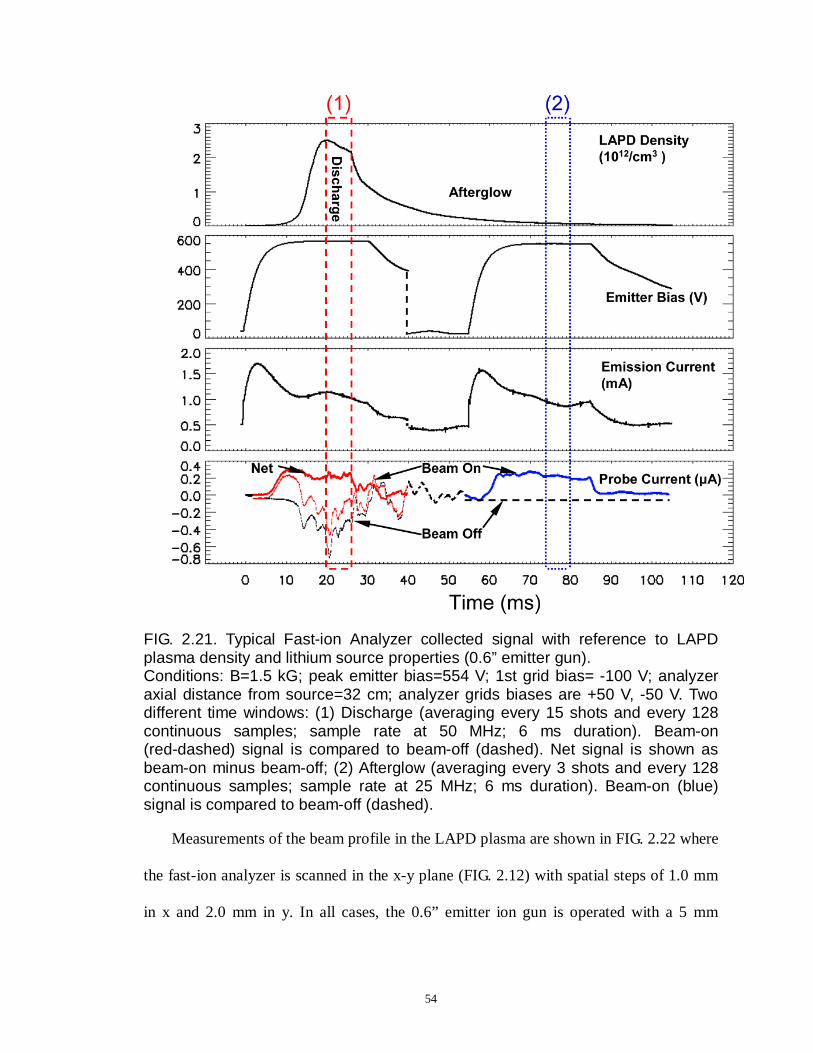
54

FIG. 2.21. Typical Fast-ion Analyzer collected signal with reference to LAPD plasma density and lithium source properties (0.6” emitter gun). Conditions: B=1.5 kG; peak emitter bias=554 V; 1st grid bias= -100 V; analyzer axial distance from source=32 cm; analyzer grids biases are +50 V, -50 V. Two different time windows: (1) Discharge (averaging every 15 shots and every 128 continuous samples; sample rate at 50 MHz; 6 ms duration). Beam-on (red-dashed) signal is compared to beam-off (dashed). Net signal is shown as beam-on minus beam-off; (2) Afterglow (averaging every 3 shots and every 128 continuous samples; sample rate at 25 MHz; 6 ms duration). Beam-on (blue) signal is compared to beam-off (dashed).

Measurements of the beam profile in the LAPD plasma are shown in FIG. 2.22 where

the fast-ion analyzer is scanned in the x-y plane (FIG. 2.12) with spatial steps of 1.0 mm

in x and 2.0 mm in y. In all cases, the 0.6” emitter ion gun is operated with a 5 mm

55

aperture. FIG. 2.22 (a) displays the transverse beam profile for a zero pitch angle beam in

the afterglow plasma, 2.5 cm from the ion gun. FIG. 2.22 (b) is a beam contour taken

during the afterglow plasma [time window (2) in FIG. 2.21]. It was found in our previous

fast-ion beam investigations 2 with argon ions, that, for helical beams, the slightly

divergent beam emanating from the gun is refocused at integer numbers of gyro orbits.

Therefore, orbits are always selected to complete integer numbers of gyro orbits that

coincide with the location of diagnostic ports. In FIG. 2.22 (b) the beam has completed

approximately one gyro orbit before reaching the analyzer at one port away (32 cm)

along the z direction. The beam spot is elongated in the direction of gyro motion. A likely

explanation for this effect is that, due to a finite energy spread, ions with different axial

velocities take different amounts of time to reach the z position of the detector. The gyro

phase φ at the detector is vcos

f z

θΩ ∆

, where fΩ is the cyclotron frequency, z∆ is the

fast-ion traveled distance in the z direction, v is the fast-ion speed and θ is the fast-ion

pitch angle. Since fΩ is independent of energy, ions with different energies reach the

detector with different gyro phases. The variation in gyro phase with energy, φ∆ , can be

expressed as

38 cosf fm z

EE

φ θΩ ∆

∆ = ∆ , (1)

where fm is the mass of lithium fast-ion and E∆ is the variation of fast-ion energy.

For a 20 eV beam energy spread, using parameters in FIG. 2.22 (b), the variation is 6.5

degrees in gyro phase and 0.31 cm in beam height along the gyro orbit. This results in the

extra spread along the gyro direction. In contrast, the radial beam width is determined

primarily by the emitted radius of the beam.

56

FIG. 2.22. Contours of 0.6” emitter gun beam profile in the LAPD plasma (color bars in µA; origin at LAPD machine center). White solid circle: 0.5 cm diameter aperture (ideal beam spot); Black cross hair: beam center; Black dash ellipse: ellipse with semimajor and semiminor axes calculated from 2D Gaussian fit of beam contour; White dash curve: part of the beam orbit projection of x-y plane with theoretical radius of 2.73 cm; White long dash line: radial line connecting beam center and orbit center.

57

The curvature of the gyro orbit at the beam collection point causes a small portion of

the beam to be absorbed on the probe wall before reaching the recessed collector, which

is the vignetting effect discussed in Ref. [18]. Since the analyzer is always rotated in the

y-z plane to match the incoming beam, the collector effective aperture in the y direction

is close to the collector diameter of 3.2 mm. The collector effective aperture in the x

direction is determined to be ~ 2.7 mm by a simulation of an ensemble of fast-ion orbits

in the analyzer geometry in the x-z plane. If a perfect 5 mm diameter beam is collected in

this manner, the widths of the beam along the x and y directions, convoluted with the

collector effective aperture, are 5.7 mm and 5.9 mm respectively.

To analyze the radial beam profile, the white dash curve is first fitted in FIG. 2.22 (b)

to indicate the beam trajectory in the x-y plane with a radius of 2.7 cm that is calculated

from the beam launching conditions. Then the profile data are extracted along radial lines

and fitted to Gaussian distributions with the goodness of fitting (χ2) recorded as statistical

weights 3. An example of a radial line is shown in FIG. 2.22 (b) connecting the cross hair

and the orbit center.

Radial profiles of the beam are shown in FIG. 2.23 for the discharge and the afterglow

signals. Both profiles are weighted averages of all the available radial lines with

sufficient signal intensity. The profiles are accurately represented by Gaussian

distributions. The error bars correspond to temporal fluctuations of beam local intensity

and they are calculated by taking standard deviations (STD) of 60 continuous time bins

(0.1 ms) of beam intensity at each radial location. The discharge beam signal is noisier

than the afterglow signal. The full width at half maximum (FWHM) for each curve is

close to the expected beam collection width.

58

FIG. 2.23. Weighted average radial beam profile in the discharge and the afterglow. r=2.7 (cm) corresponds to the predicted center of the gyro orbit. The horizontal line indicates the FWHM for each curve.

59

2.5.2 B-dot Probes for Wave Magnetic Field

The wave magnetic field is measured by a set of identically designed b-dot probes

featuring three orthogonal induction coil-pairs which are sensitive to the time derivative

of the wave magnetic field19. Each coil-pair is connected to a differential amplifier to

select magnetic signal and reject common mode noise. The calibration information of the

ten b-dot probes is in Appendix D. During the experiments, the magnetic coils are

oriented so that the three components of the wave field align with the LAPD coordinate

system.

FIG. 2.24. An example of the orthogonal coils in a b-dot probe. (Figure from S. Vincena Ph. D. thesis)

60

1 http://www.cscamm.umd.edu/cmpd/lapd.htm

2 H. Boehmer, D. Edrich, W.W. Heidbrink, R. McWilliams, and L. Zhao, Rev. Sci. Instrum., 75,

1013 (2004).

3 L. Zhao, W.W. Heidbrink, H. Boehmer, R. McWilliams, Phys. Pl. 12, 052108 (2005).

4 Y. Zhang et al., Bull. Am. Phys. Soc. FP1.00075 (2005).

5 M. Sasao, K. A. Connor, K. Ida, H. Iguchi, A. A. Ivanov, M. Nishiura, D. M. Thomas, M. Wada,

and M. Yoshinuma,IEEE Trans. Plasma Sci., 33(6), 1872(2005).

6 J. P. Blewett, Ernest J. Jones, Phys. Rev., 50, 464(1936).

7 G. E. Sasser, S. F. Knowlton, R. F. Gandy, H. Lin, E. E. Thomas, and M. A. Owens, Rev. Sci.

Instrum., 66(1), 324 (1995).

8 D. C. Pritchard, R. F. Gandy, J. D. Hanson, S. F. Knowlton, H. Lin, G. E. Sasser, E. Thomas, Jr.,

and J. Cooney, Phys. Plasmas, 4(1), 162 (1997).

9 D. M. Thomas, A. S. Bozek, J. I. Robinson, K. H. Burrell, T. N. Carlstrom, T. H. Osborne, R. T.

Snider, D. K. Finkenthal, R. Jayakumar, M. A. Makowski, D. G. Nilson, and B. W. Rice, Rev. of

Sci. Instrum. 72(1), 1023(2001).

10 R. J. Fonck, P. A. Duperrex, and S. F. Paul, Rev. of Sci. Instr. 61(11), 3487(1990).

11 G. McKee, R. Ashley, R. Durst, R. Fonck, M. Jakubowski, K. Tritz, K. Burrell, C. Greenfield, and

J. Robinson, Rev. of Sci. Instr. 70(1), 913(1999).

12 D. M. Thomas, Rev. of Sci. Instr. 66(1), 806(1995).

13 A. Theodore Forrester, Large Ion Beams—Fundamentals of Generation and Propagation

(Wiley,1988).

14 Heat Wave Labs, Inc. alkali ion source doc. http://www.cathode.com/pdf/tb-118.pdf

15 H. B. Haskell, O. Heinz, D. C. Lorents, Rev. Sci. Instrum., 37(5), 607 (1966).

16 W. Gekelman, S. Vincena and D. Leneman, Plasma Phys. Control. Fusion 39, A101 (1997).

17 Walter Gekelman, Stephen Vincena, David Leneman, James Maggs, J. Geophys. Res. 102, 7225

61

(1997).

18 W. W. Heidbrink, J. D. Strachan, Rev. Sci. Instrum. 56, 501 (1985)

19 D. Leneman, W. Gekelman, and J. Maggs, Phys. Plasmas 7 (10), 3934 (2000).

62

C h a p t e r 3

CHAPTER 3 FAST-ION DOPPLER SHIFTED

CYCLOTRON RESONANCE WITH

SHEAR ALFVÉN WAVES

This chapter presents the direct experimental measurement of fast-ion cross-field

transport induced by SAWs in the linear regime.

• Sec. 3.1: Analytical resonance theory

• Sec. 3.2: SAW dispersion relation

• Sec. 3.3: Simulation codes

• Sec. 3.4: Experimental setup

• Sec. 3.5: Resonance results

63

3.1 Resonance Theory

A charged particle is in cyclotron resonance with a transverse wave if the oscillation

of wave electric field E matches the Doppler-shifted cyclotron motion of the particle1,

when the particle and the wave exchange energy effectively. The condition for such a

resonance between fast ions and SAWs propagating parallel to the ambient magnetic field

B0 (along the z direction) is

vz z fkω − ≅ ±Ω , (3.1)

where ω and kz are the wave frequency and parallel wave number; vz is the parallel

velocity of the fast ions in the lab frame; and Ωf = qfB0 / mf is the cyclotron frequency of

the fast ions. For MHD shear Alfvén waves, the dispersion relation is ω = kz vA with

0 0v /A i iB n mµ= as the wave phase velocity (the Alfvén speed), nimi is the mass density

of the plasma. The upper/lower sign in Eq. (3.1) corresponds to the normal/anomalous

Doppler resonance where fast ions travel slower/faster than the wave phase velocity along

B0. In the following experiments, normal Doppler resonance is investigated. The goodness

of the resonance is first evaluated by this normalized difference

( )v / 1z z f fkω ω∆ = − −Ω Ω . (3.2)

The position x and velocity v of the fast ion is given by the Lorentz force law,

( )0f

f

qd

dt m

d

dt

= + × + × =

vE v B v B

xv

, (3.3)

where E and B are the wave fields of SAW. Adopting Cartesian coordinates, the wave

64

electric field can be modeled as linearly polarized in the y-z plane,

( ) 0ˆ ˆ( , , ) E E cos( v )y z z zy z t y z t kω ϕ= + − +E , (3.4)

where φ0 is the launched phase of the fast ion relative to the wave and assuming E 0x = .

From Ampere’s law, Ey is related to Bx

through:

BE - z x

y

k

ωµε=

, (3.5)

where µε is determined by the plasma dispersion relation (Sec. 3.2). In the experiment,

Ey has a perpendicular pattern determined by the characteristics of the SAW antenna

(see Sec. 3.4.4). Replace B in Eq. (3.3), then the changes of fast-ion velocity

components become

( )0

0

vv B

vv B 1 v E

vE v E

fxy

f

y fx z y

f z

fzz y y

f z

qd

dt m

d q

dt m k

qd

dt m k

ωµε

ωµε

= × = − × + − ⋅ = + ⋅

, (3.6)

which shows that perpendicular acceleration is only along the y direction, and that the

parallel acceleration is associated with the rate of change of perpendicular kinetic energy1,

as well as acceleration from Ez . At the exact Doppler resonance condition, vy grows

linearly with t. The phase of Ey seen by the fast ion changes and eventually turns

opposite, when the fast ion accelerates in the opposite direction. The amplitudes of the

parallel and perpendicular velocities undergo slow oscillations over time and space much

longer compared to the period and wavelength of the wave. This oscillation is actually the

fast ion’s trapping in the SAW. From Ref. [1], the trapping period (τtrap) can be calculated

65

as

trap 20

8

E vf

z f y z

m

k q

π ωτ = , (3.7)

where v0z is the initial parallel velocity. The distance traveled along the z direction in tTrap

is defined as λtrap, the trapping length.

The Landau resonance is another resonance mechanism for the fast-ion beam to

exchange energy with the SAW. The resonance condition for this case seems conceptually

simpler than the Doppler resonance:

v 0z zkω − ≅ . (3.8)

However, it requires a fast Li+ ion (> 2 keV) at a relatively small initial pitch angle, which

is currently not an operational regime for this thermionic emission source (see Sec. 2.3.1).

One example of the Landau resonance condition is listed in Table 2, where the plasma

conditions are modified from usual LAPD operations in order to slow down the wave.

3.2 SAW Dispersion Relation

There are two regimes of plasma parameters for SAW propagation: the Kinetic

Alfvén Wave (KAW) for plasma electrons having a Boltzmann distribution in the

presence of the Alfvén wave fields and the Inertial Alfvén Wave (IAW) for electrons

responding inertially to the wave. The KAW is more relevant to the physics of the

interior regions of tokamak plasmas and the IAW to the edge and limiter regions. In this

experiment, KAWs launched during the discharge of the LAPD are investigated.

A dimensionless parameter— 2 2v / ve te Aβ ≡ is a quantitative measure of how inertial

66

or kinetic a plasma region is, where v 2 /te e eT m= is the thermal electron speed with Te

the electron temperature. If 1>>eβ , as in the discharge plasma of the LAPD, it is

kinetic; if 1<<eβ , as in most of the afterglow, inertial. For the KAW, the dispersion

relation is

2 2 2 2 2 2/// v (1 ),A sk kω ω ρ⊥= − + (3.9)

where k// is the component of the wave vector parallel to the background magnetic field, ⊥k is the

perpendicular wave number and sρ is the ion sound gyro-radius ciss c ωρ /= with

( ) 2/1/ ies mTc = . The intensity of the parallel wave electric field is13

2

// 2 2 2 2 1/2v (1 )(1 )s

A s

i k

k

ω ρω ω ρ

⊥⊥

⊥− − +E = E . (3.10)

A typical ratio of / /

⊥

EE

is 0.01, which means that the non-vanishing parallel electric field

will modify vz in the resonance experiment. The perpendicular electric field can be

calculated from Ampère’s law and the dispersion relation:

2

2 2 2 1/2

v (1 )

(1 )A

sk

ωω ρ

⊥

⊥ ⊥

−

− +

E=

B

. (3.11)

3.3 Resonance Orbit Simulation Code

3.3.1 Single particle simulation

If the cross field transport of the test-particle beam is much smaller than the scale

67

length of the wave fields, then a single particle Lorentz code is capable of predicting the

expected resonance beam profile by launching particles at an ensemble of initial phases

(φ0).

In the plasma physics literature, cross-field diffusion usually refers to radial transport

of guiding centers. In this experiment, the fast ions only execute a few Larmor orbits

prior to measurement, so it is conceptually simpler to examine the full helical Lorentz

orbit rather than the guiding-center orbit. A typical Doppler resonance fast-ion trajectory

is shown in FIG. 3.1 a). Fast ion and wave parameters (Table 2) are chosen to satisfy the

Doppler resonance condition of ω∆ < 0.1, using feasible experiment conditions. To

indicate the relative strength of different SAWs, Bmax is defined as the maximum

amplitude of Bx in a specific z plane. If max ˆB Bx x=

at t = 0, the ions, initiated in phase

with the wave, would lose energy (FIG. 3.1 b) continuously from the wave and the

magnetic moment ( 2v / 2m Bµ ⊥= ) decreases. At several gyro-cycles away in the z

direction, the fast-ion energy (W) and µ changes linearly with the traveling time/distance;

as W changes, the initial phase φ0 will eventually change to 0ϕ π± , when W starts to

change in the opposite direction. The trapping length (λtrap) is ~ 46 m from the original z

position (FIG. 3.1 b). The fast ion oscillates in phase space over long periods—the

trapping of fast ions in the wave frame.

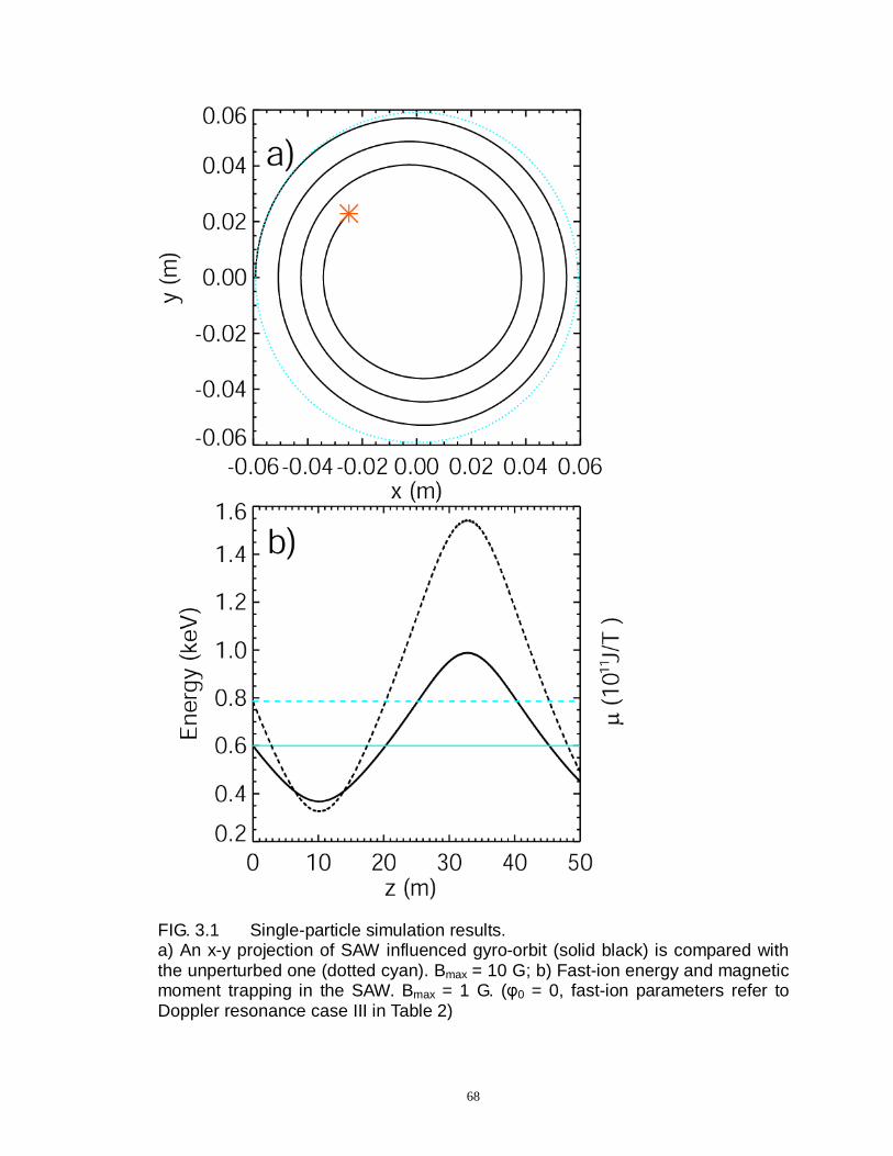
68

FIG. 3.1 Single-particle simulation results. a) An x-y projection of SAW influenced gyro-orbit (solid black) is compared with the unperturbed one (dotted cyan). Bmax = 10 G; b) Fast-ion energy and magnetic moment trapping in the SAW. Bmax = 1 G. (φ0 = 0, fast-ion parameters refer to Doppler resonance case III in Table 2)

69

If an ensemble of ions are launched with random phases relative to the wave,

0 [0,2 ]ϕ π∈ , other initial conditions being identical, their positions on the collection plane

mark the spatial spreading caused by the perturbation from the wave field (FIG.3.2 a). The

maximum displacements from the undisturbed position along the r and φ directions

are defined as ∆r and r0∆Φ. It is obvious that ∆r is a direct indicator of the change in

perpendicular ion energy (W). The gyro phase Φ at the collection plane is vf

z

zΩ ∆, where

z∆ is the distance traveled by fast ions in the z direction. Thus r0∆Φ indicates the change

in parallel energy (W//).

70

FIG.3.2. Single-particle simulation results, cont. a) Fast ion collection positions at ∆z = 0.96 m with 16 uniformly distributed values of initial wave phase φ0 (color crosses). Black box is the unperturbed collection position. Bmax = 1 G; b) Doppler resonance spectra of ∆r at variable z and Bmax. (Fast-ion parameters refer to Doppler resonance case III in Table 2)

71

In the simulation, varying the wave frequency from 0.1 to 1.0 ωci (singly-ionized

helium ion cyclotron frequency), one can obtain the spectrum of spatial displacements

caused by the SAW perturbation. In FIG.3.2 b) ∆r and r0∆Φ are plotted against

/ ciω ω ω= , where the frequency satisfying the resonance condition ( ω∆ = 0) is 0.65 ωci.

Resonance spectra show that the maximum displacement occurs at the expected frequency.

At larger ∆z (less than λtrap/4), the resonance frequency is closer to 0.65 ωci and the

resonance peak is sharper. At shorter lengths, e.g. several gyro-cycles away, the quality

factor of the resonance is degraded but a clear maximum is still observed. The spatial

displacements are proportional to the SAW wave field amplitude, as expected for

moderate field perturbations (δB / B < 1%) in the linear regime.

The simulation code was first used to find the optimal conditions for conducting the

resonance experiments with fast-ion sources in the LAPD. Realistic ranges for parameters

listed in Table 2 are evaluated in the code for ω∆ , ∆r and r0∆Φ. Those sets of parameters

satisfying 1ω∆ while producing observable ∆r and r0∆Φ are selected for experiments

at the LAPD. Three lithium fast-ion Doppler resonance conditions in Table 2 are realized

and measured experimentally. In this article, if not otherwise specified, the resonance

parameters are for 7Li + Doppler resonance case (III).

72

Resonance Parameter

7Li +

Doppler (I) 7Li +

Doppler (II) 7Li +

Doppler (III) Li+7 Landau

B (kG) 1.6 1.74 1.2 0.5

W (eV) 600 600 600 2000

θ (deg) 29.5 44.8 49.3 15

ρ (cm) 2.9 3.8 5.9 8.2

Gyro-cycle/port 1/1 4/3 1/1 1/6 ne (1012 cm-3) 2.0 2.5 2.5 4

Te (eV) 6 6 6 4

fci (kHz) 610 663 457 191

∆r (cm) (∆z = 0.96 m)

0.43 0.5 0.5 n/a

Resonance ω 0.63 0.63 0.65 128

Table 2 List of parameters for typical cases of fast ion and SAW resonance.

3.3.2 Monte-Carlo simulation

Since the single-particle model cannot simulate a finite beam with spatial and energy

distributions, an existing Monte-Carlo fast-ion orbit code2 is upgraded to include the

SAW induced fast-ion transport, as well as the classical transport caused by thermal ions

and electrons. In the LAPD discharge plasma, the electrons dominate Coulomb

slowing-down, while thermal ions dominate the pitch-angle scattering rate. A number of

fast ions are launched numerically according to the initial beam divergence in phase

space (±5 deg. in pitch angle and ~ 5 eV in energy). Due to the difference in time scales

of the transport mechanisms shown in Table 3, the classical transport effects can be

73

readily de-coupled from the SAW influence.

Transport Time Scales Time (ms) Pitch angle scattering: τPAS 5

Coulomb energy-loss: τW 1

SAW period: τSAW 0.002 – 0.02

Cyclotron Motion: τCyclotron ~ 0.003

Table 3 Comparison of time rates for different transport mechanisms. B0 = 1.2 kG

During the simulation of each fast-ion orbit, the pitch angle scattering event is

considered at a randomly selected time (t = t1), by which each gyro-period is divided into

two partitions (τCyclotron = t1 + t2). FIG.3.3 shows the flow chart of the simulation process.

The single-particle Lorentz code is carried on throughout t1 and t2 for SAW perturbation.

At the end of each time partition, the fast-ion energy is updated by the Coulomb

slowing-down effect:

' expW

tW W

τ

= − . (3.12)

At t = t1, a Monte-Carlo collision operator2 developed from the Coulomb scattering

theory3 is loaded to scatter the direction of the fast-ion velocity without changing its

magnitude. After the desired number of gyro-periods is finished, the fast-ion velocity and

coordinates are recorded in the computer memory and next fast-ion orbit is launched.

74

FIG.3.3 Monte-Carlo simulation flow chart

75

Using the same linearly polarized shear Alfvén wave fields as for the single-particle

simulation, thousands of fast-ion orbits are launched with random phases (φ0) to

contribute to the beam profile several gyro-cycles away. The SAW-perturbed beam

profiles are compared in FIG.3.4 with the classical profiles at different distances traveled

by fast ions. Notice in FIG.3.4, all the fast ions collected in the x-y plane are included

regardless of their final velocities. The classical beam profile produced by a 0.5 cm

diameter source aperture is shown in FIG.3.4 a). For the SAW-perturbed beam profiles,

Bmax is set at 10 G. At the resonance peak frequency (FIG.3.4 b, ω = 0.65), substantial

profile widening happens along both the r (gyro-radius) and φ (gyro-angle) directions.

The widening effect increases with the distance traveled by the fast ion. At the resonance

null frequency (FIG.3.4 c, ω = 0.20), on the contrary, fast ions only perform drifting

motions along with the guiding center, whereas the gyro-radius as well as the

perpendicular energy doesn’t change much. At ∆z = 0.32 m and 0.64 m, beam profiles at

different phase (φ0) form a ellipse. At ∆z = 0.96 m, where fast ions finish 3 gyro-cycles,

beam profile (FIG.3.4 c) has minimal drifting and is close to the unperturbed one in

FIG.3.4 a). These results from the Monte-Carlo model agree with the experimental

findings in Sec. 3.5.

76

FIG.3.4. Monte-Carlo model simulated fast-ion beam profiles with different SAW perturbations. The color of the dots indicates fast ion collection at different z planes: black (∆z = 0 m), blue (∆z = 0.32 m), green (∆z = 0.64 m) and orange (∆z = 0.96 m). (a) no SAW present; (b) SAW at ω = 0.65 (resonance peak), Bx

= 10 G; (c) SAW at ω =

0.20 (resonance null), Bx = 10 G.

3.4 Resonance Experimental Setup

3.4.1 Overview

This experiment is performed in the upgraded LAPD, which has a 17.56-m-long,

1-m-diameter cylindrical main vacuum chamber. Pulsed plasmas (~ 10 ms in duration, 1

Hz repetition rate and ±10% spatial uniformity) are created by a discharge between a

barium oxide coated cathode and a gridded molybdenum anode4. The cathode and anode

are separated by 50 cm and are both located at the south end of the machine. The working

gas is helium at a partial pressure ~ 3 x 10-5 Torr with less than 3% of impurities. Typical

77

average plasma parameters for this experiment are: ni ~ 2.5 x 1012 cm−3, Te ~ 6 eV, Ti ~ 1.0

± 0.5 eV.

FIG.3.5. Experimental setup at the LAPD. a) Overview of instruments; b) ambient magnetic field profile versus LAPD port number. The distance between two adjacent ports is 0.32 m. Instruments’ typical locations are marked by dashed perpendicular lines.

FIG.3.5 a) illustrates the hardware configurations for this experiment. The origin of

the z axis is defined as the location of the lithium fast-ion source (Sec. 2.3.1). The

beam-wave interaction region is ~ 10 meters downstream of the cathode to ensure

radially uniform background plasma properties. The SAW antenna (Sec. 2.4) is located at

z = - 3.52 m to avoid the near field effect (typical SAW wavelength parallel to B0 is ~ 4

m). The fast-ion analyzer (Sec. 2.5.1) scans fast-ion signals in the x-y plane 0.32 to 0.96

m away from the source to vary the interaction time between wave and particle. FIG.3.5 b)

shows the actual LAPD port locations of all the instruments relative to the ambient

78

magnetic field profile. The distance between two adjacent ports is 0.32 m. One set of

magnets next to the anode-cathode carries a higher current corresponding to a 1.4 kG

field to avoid strong Alfvén maser formation5 which is a major source of wave field

noise. A dissipating magnetic beach on the north end of the machine is used to suppress

reflection of the waves at the end of the machine. The axial magnetic field profiles are

calculated from the actual current distribution for all the magnets in the machine6. The

estimated axial field ripple amplitude at the radius of the machine is less than 2% for a

constant field configuration.

3.4.2 Fast-ion Signal Detection

The stainless steel source outer-shield (3” x 5”) changes local plasma parameters

(especially when the outer shield is grounded to the LAPD chamber as is preferred). A

measurement of plasma floating potential (Vf) near the source region shows up to 10 V of

decrease, which causes a small adjustment of the beam energy. SAWs launched from

inserted antennas can also be influenced if the source is aligned axially with the

oscillating current channels that create the wave (Sec. 3.4.4).

A special synchronization between the lithium source and the LAPD plasma is

employed, so that the ~ 20 ms fast-ion pulse is turned on and off every two plasma

discharges, with an adjustable delay and duration. The background signal is taken when

the source is disabled for one shot right after the previous beam-on shot. Even number of

shots is repeated at one spatial location before the probe drive moves on. The signals with

the source on are subtracted by the signals with the source off. The fast-ion signals shown

in this work are net signals with background subtractions.

79

An electrical diagram for the experiment is shown in FIG.3.6. Apart from the Alfvén

Maser signal, which is usually avoided as stated earlier, there exist two major noise

sources: the ~ 6 kA plasma discharge pulse causes ringing signals at 1 – 1000 Hz due to

capacitive and inductive couplings; the SAW rf driving-circuit generates EM noise

outside of the chamber as well as SAW propagation inside the plasma. It is thus very

important for the lithium source to have a solid ground reference to the LAPD chamber

ground with a complete shield around the heating and biasing circuit. Two Mu-metal

shielded high-voltage power supplies7 bias the emitter and the accel-decel grid at desired

voltages with < 0.05% ripple rate (< 0.3 Vpp ripple at 600 V), monitored by a Tektronix

P6015A high voltage probe.

80

FIG.3.6 Electrical configurations and shielding solutions for fast-ion generation

and diagnostics.

(Drawings are topologically correct but not to scale.)

After the beam travels in the plasma/wave fields, a collimated fast-ion analyzer is

employed to produce a good fast-ion signal-to-noise under strong rf noise environment

during the LAPD discharge. It packages a 3.2 mm dia. collector, an identical dummy for

differential amplification and three molybdenum grids for variable electrical barriers.

Typical probe current signals are in the 0.1 - 1 µA range at large distances from the ion

gun. At operational pitch angles for the source (> 28˚), the tubular housing is directed

parallel to the local ion beam trajectory (FIG.3.5 a), in which the collector is recessed by

81

more than the plasma ion Larmor radii to block thermal particles’ entrance geometrically.

The second grid is biased positive (~ + 50 V) and the first grid is biased negative (~ - 10

V) to further reject plasma ions and electrons electrically. Another application of the

analyzer is to sweep the bias of the second grid up to 800 V to obtain the energy

distribution of the ion beam. For a 600 eV beam with a pitch angle of 28º, measured 1”

away from the beam exit in the LAPD afterglow plasma, the energy spread (3%) is

similar to that measured in a vacuum magnetic field. A continuous low-energy tail in the

energy distribution function is observed in the distribution in the presence of the plasma.

The fast-ion current and the dummy pickup signal are fed through a RG 178B/U

coaxial cable twisted pair, shielded by the stainless 0.95 cm O.D. shaft. Due to the shaft

length that’s required by the LAPD standard probe drive as well as a minimum of ~ 1 m

for external connection, the total capacitance of each coaxial signal line is ~ 270 pf. For

this work, a 1 MΩ input resistance is needed for sufficient fast-ion signal as well as for

filtering out strong rf pickups. Signals are pre-amplified by a Lecroy DA1822A

differential amplifier. A SONY/Techtronix A6907 optical isolator separates the fast-ion

current reference and the data collection ground, reduces the offset caused by the plasma

discharge, and amplifies the beam signal for the 100 MHz, 8 bit digitizer.

Measurements of the beam profile and wave field utilize a 2D probe drive system (±

0.5 mm precision) and highly reproducible plasma shots of the LAPD. At each spatial

location, multiple time traces are collected with a number of plasma shots repeated. The

probe tip is then moved to the next spatial position according to the pre-selected grid and

the process is repeated.

The fast-ion signal data and other channels such as the SAW antenna current are

82

collected simultaneously by a computer controlled digitizer board. A Labview program

controls the data collection sequence including timing and triggering, probe driving, and

antenna frequency sweeping. HDF5 formatted files are compiled after each data run to

document all the fundamental information including the plasma discharge current and

density, chamber partial pressures, cathode temperature, interferometer trace and

magnetic field configuration. A typical fast-ion profile during the discharge of the LAPD

plasma is reconstructed from the data array and shown in FIG.3.7. The collimated fast-ion

analyzer has good fast-ion signal-to-noise and spatial resolution.

83

FIG.3.7. A typical lithium fast-ion beam profile during the discharge of the LAPD plasma, with superimposed curves to aid further analysis. Fast-ion analyzer located at z = 0.96 m. Gaussian center of x profiles: white diamond; Fitted gyro-orbit from Gaussian centers: white-dashed; Radial cuts every 1 degree: white-dotted; Minimum and maximum radial range: white-solid.

84

3.4.3 SAWs Launched by Loop Antenna

The LAPD’s large physical size and sufficiently high plasma density and magnetic

field accommodates multiple Alfvén wavelengths. Research on SAW properties in the

LAPD dates back to 1994 when pairs of theoretical8,9 and experimental10, 11 papers were

published on SAWs radiated from small perpendicular scale sources in the LAPD.

Subsequently, other mechanisms were discovered to generate Alfvén waves including a

variety of inserted antennas, resonance between the LAPD cathode and the

semi-transparent anode—the Alfvén Maser5, and a dense laser-produced plasma

expansion12. In 2005, Palmer13 measured thermal ion polarization and 0×E B drifts

caused by SAW fields.

To date, there are two different SAW perpendicular modes that are actively launched

from inserted antennae in the LAPD. An azimuthally symmetric SAW pattern (m = 0)

with ⊥E along the radial direction can be excited by direct application of an oscillating

charge density to a flat, circular mesh (r ~ 0.5 cm) or external feeding of an oscillating

current through a thin copper rod parallel to B0. By adding another identical current

channel along B0 at the opposite phase, a few centimeters away in the x-y plane, an m = 1

mode can be excited with a linearly polarized ⊥E region near the center of two current

channels.

This work uses an insulated rectangular copper loop14 as an antenna. It is 30 cm

along B0 and 15 cm along the y axis. Currents flowing through the two parallel wires

along B0 generate an m = 1 perpendicular field pattern. The linearly polarized region of

85

the m = 1 pattern is aligned with part of the gyro-orbit to produce the Doppler resonance

effect. FIG.3.8) shows the typical alignment of the Li+ orbit and the SAW fields in the x-y

plane, where the resonant fast ion gets a “kick/drag” every time it “swings” by the

maximum field region. The geometry and position of the source head is also drawn to

show that, for larger gyro-orbit condition, the source head is farther away from the SAW

current channels and has less effect on the fields.

86

FIG.3.8. Arrangement of fast-ion source (red dashed) and the SAW fields on a perpendicular plane. Electric field data (white arrows, length proportional to field intensity, maximum at 34.3 V/m) are calculated from measured magnetic field data ( Bx

shown by color contour) taken at z = 0.64 m. f = 297 kHz. The unperturbed fast-ion orbit is the black dashed circle.

87

Two different circuits drive the loop antenna. The primary rf supply drives up to 2 kA

through the loop and generates Alfvén wave amplitudes up to 10 G at variable

frequencies up to 0.8 ωci (FIG.3.8). An Ethernet controlled Agilent waveform-generator

manages the frequency of the output SAWs. The current wave form is triangular and

contains harmonics of the fundamental. Since the SAWs are expected to be strongly

damped near and above ωci,15 the harmonics are usually inconsequential but do affect

waves launched at fundamental frequencies lower than 0.3 ωci. The secondary driving

circuit produces a nearly sinusoidal wave form but requires matching capacitors for each

SAW frequency. It produces amplitudes up to 1 G. In the following, the default antenna

current drive is the triangular one unless otherwise noted.

FIG.3.9. Spectra of Bx and loop antenna current by triangular drive.

B-dot probe signal taken at the radial center of z = - 0.32 m during Sep. 2007 LAPD run. (Data acquired with 100 MHz sampling rate, averaging 8 samples and 8 consecutive plasma shots). The fluctuations of the Bx

spectrum (FIG.3.9) as ω varies are due to the

field-line-resonance effect studied by C. Mitchell et al.16, 17. Although a flaring field at

the north end of the machine is configured to reduce this effect (FIG.3.5 b), there are still

reflected waves to interfere with the primary waves. The b-dot probes measures the linear

88

addition of all wave fields. Since only the forward wave can satisfy the normal Doppler

resonance condition, using the b-dot probe measured fields for Doppler resonance

calculation would incur systematic error which can be estimated from FIG.3.9.

3.4.4 SAW Perpendicular Pattern

FIG.3.10. Perpendicular SAW magnetic field patterns. a) port 36 (z = -0.32 m), f = 297 kHz; b) port 33 (z = 0.64 m), f = 297 kHz; c) port 31 (z = 1.28 m), f = 297 kHz; d) port 31 (z = 1.28 m), f = 154 kHz.

B-dot probes plane scans at multiple ports show that the axial variations of the wave

field perpendicular pattern are small for the same launching frequency. The influence of

the grounded fast-ion source on the wave pattern is noticeable and frequency scans at

various frequencies reveal different levels of this effect on the wave pattern near the

source. Higher frequency SAWs, corresponding to shorter parallel wavelengths, have

more distortion in the wave pattern (FIG.3.10 which section). While a generic wave

perpendicular pattern can be employed first to estimate the theoretical resonance effect,

simulations using experimental wave field data for different frequencies are still

necessary to make careful comparison between theory and experiment (Sec. 3.5.2).

89

3.5 Resonance Experiment Results

3.5.1 Fast-ion Signal Shows SAW-Induced Transport

As discussed earlier, the ~ 20 ms fast-ion beam pulse is turned on and off every two

LAPD plasma discharges. Close to the end of each discharge, the plasma parameters

reach the best uniformity in time and space, when the loop antenna drives an adjustable rf

current for 0.5 – 0.8 ms, launching SAWs at the specified frequency. When the beam

pulse is on, it overlaps in time with the 10 ms LAPD discharge. The data collection

time-window opens for 2 ms with ~ 0.5 ms before and after SAW duration. A typical time

history of a Doppler resonance experiment is shown in FIG.3.11, with SAWs launched at

the resonance frequency (297 kHz for Doppler resonance case III). The triangular wave

form of the SAW current is magnified in the inset of FIG.3.11 c). Fast-ion net signals are

shown in FIG.3.11 a) and b) where the source is pulsed on for the whole ~ 2 ms window.

The fast-ion signals in FIG.3.11 a) and b) change significantly in intensity, towards

different directions, when SAWs propagate to the location of the fast-ion orbit several

microseconds after current drives through the antenna. The spatial locations of the two

time traces are different: a) is taken at the center of the beam spot whereas b) is near the

edge, which are accurately indicated in FIG.3.12. Since the RC time is much longer than

the SAW period, fast-ion signal variation at SAW frequency is filtered out. However the

averaged beam profile would still widen in the r and φ directions, as shown in the

Monte-Carlo simulation results (FIG.3.4). With particle conservation in mind, the fast

90

ions are transported from the center of the beam to the edge, during Doppler resonance.

This effect in experiment is shown in FIG.3.11 where the beam center/edge signal

decreases/increases when the SAW is turned on. When the SAW is turned off, the signal

restores back to the unperturbed values. The green curves in FIG.3.11 a) and b) are the

fitted RC decay/rise curves yielding an RC time of 0.3 0.05± ms, which is in agreement

with the estimated value.

In the following analysis, the SAW-influenced beam signal uses the averaged signal

from 0.6 ms after the onset of the antenna current, shown in FIG.3.11 a) and b) with the

red-dashed time window. This average has underestimation of the signal change if the

SAW-influence time was infinite, which means the actual fast-ion transport effect in the

experiment is up to ~ 8% more significant than shown by the current data. The

unperturbed beam signal, as a reference, is the average over the blue-dotted time window

before SAW-influence.

91

FIG.3.11. Typical fast-ion signal time traces influenced by SAWs at the Doppler resonance frequency. a) beam center signal RC decay; b) beam edge signal RC rise; c) Loop antenna current. Inset: magnified triangular current signal for the initial 0.5 ms. (SAW frequency 297 kHz; Data acquired with 25 MHz sampling rate, averaging 8 samples and 8 consecutive plasma shots, Dec. 07 LAPD run).

Time traces taken at a selected spatial grid are processed to show the fast-ion beam

profile at the x-y plane. Fast-ion signals with and without SAW influence show significant

difference in FIG.3.12, in agreement to the transport effect at resonance frequency. From

the 3D visualization in FIG.3.12 a), fast-ion intensity migrates from the center of the

beam to the edge, causing widening along the r and φ directions. The beam profile

92

along each direction is acquired using the statistical technique mentioned in Sec. 2.5.1.

Both profiles are widened as the SAW is turned on.

FIG.3.12. Comparison of fast-ion beam profile with and without SAW influence. a) 3D visualization of beam profiles with (gridded surface) and without SAW influence (shaded surface); b) Normalized weighted radial profiles with (red-solid) and without SAW influence (blue-dashed); c) Normalized gyro-direction profiles with (red-solid) and without SAW influence (blue-dotted) (SAW frequency 297 kHz; Data acquired with 100 MHz sampling rate, averaging 8 samples and 10 consecutive plasma shots, Sep. 07 LAPD run).

93

3.5.2 Measured Doppler Resonance Spectra

In this section, quantitative agreement between the measured and predicted resonant

spatial broadening is demonstrated. The resonance spectra of SAW-induced

displacements are measured and compared with the theoretical spectra.

Based on the theoretical spectra in FIG.3.2 b), a set of SAW frequencies is selected to

cover the important features of the spectra, e.g. peaks and nulls of the resonance. For

each of these frequencies, the antenna is driven for multiple plasma shots (8 – 10) and

fast-ion signals are taken at the same spatial location. After completing all the frequencies

and shots, the fast-ion analyzer is moved to the next point on the x-y grid. The total time

of the spectra measurement is usually kept within 2 hours (~ 1/10 of source lifetime) to

avoid significant change in the lithium source performance.

The spatial profile at each frequency is acquired from the data array and analyzed as

shown in FIG.3.7. As mentioned in Sec. 3.3, both ∆r and r0∆Φ are measurable indicators

of the resonance effect and ∆r is more favorable, which corresponds to the change in the

perpendicular fast-ion energy. In FIG.3.13 a), a typical set of radial profiles for the

selected frequencies (colored) are shown, to which the classical profile (black-dashed) is

compared. The fast-ion migrating effect varies as the frequency, which peaks at 0.65 ωci

and diminishes at 0.20 and 0.41 ωci, as expected from the theory. In FIG.3.13 b) and c),

plotted are the frequency dependences of full-width-half-maximum (FWHM) and the

beam intensity coefficient (P0) calculated from the Gaussian fit of the profile:

94

20

0 2

( )( ) exp c

r rP r P P

b

−= − + , (3.13)

where P is the radial profile, b is proportional to the FWHM and Pc is the background

level. It is obvious that the variations of both quantities have similar dependence on ω

as expected.

95

FIG.3.13. a) Fast-ion beam radial profiles with various SAW frequencies (colored lines/symbols) compared to the unperturbed profile (black-solid); b) Changes in FWHM of beam radial profiles versus SAW frequency; c) Changes in Gaussian peak intensity (P0) versus SAW frequency. (Data acquired with 25 MHz sampling rate, averaging 8 samples and 8 consecutive plasma shots, Dec. 07 LAPD run).

96

In order to determine ∆r quantitatively from the experimental beam profile, the

profile WITHOUT SAW is displaced digitally to find an empirical ∆r that produces the

best fit of a specific profile WITH SAW. The single-particle result in FIG.3.2 a) shows

that the fast-ion collection position undergoes elliptical displacements with SAW

perturbations at different phases (φ0). The projection of the SAW displaced beam center

(rSAW) along the r direction can be thus modeled by:

0 0sin( )SAWr r r ϕ= + , (3.14)

where r0 is the classical radial position and ∆r is as defined in Sec. 3.1. Then the

integration of all the displaced profiles across the region of 0 [0,2 ]ϕ π∈ yields an

empirical profile that is dependent on ∆r. If such a profile has the best χ2 fit to a SAW

perturbed profile, then the corresponding ∆r is regarded as the displacement inferred from

experimental data (FIG.3.14). For well-behaved Gaussian distributions like the beam

classical profiles in Eq. 3.13, that integration can be written as

( ) 2 20

0 020

( sin( ))1, exp

2 c

r r r tP r r P P d

b

π ω ϕπ

− − ∆∆ = − + ∫ . (3.15)

This algorithm converges rapidly as φ0 integration step goes below 2π/100.

97

FIG.3.14. Illustration of widened beam spot caused by beam displacement along the r direction.

FIG.3.15 shows the Doppler resonance spectra of calculated ∆r from measured

fast-ion beam profiles. For Doppler resonance case III, two different sets of data acquired

during two LAPD runs (Sep. and Dec. 2007) are plotted in FIG.3.15 a), both using the

triangular wave drive at similar intensities. The single-particle model using a generic

wave field pattern produces the continuous theory curve. The measured wave field

amplitude spectrum (FIG.3.9) is used in the simulation. Although slightly different in the

wave field strength and the source-antenna arrangement between the Sep. and the Dec.

run, the resonance spectrum is similarly characterized by both data sets. The absolute

magnitude of ∆r shows good agreement between experiment and theory. In FIG.3.15 b),

Doppler resonance case II is plotted with its own theoretical resonance curve. Agreement

is still good even though this case has smaller fast-ion gyro-radius (3.8 cm) and the

source has more perturbation on the SAW field pattern (FIG.3.10).

98

FIG.3.15. Doppler resonance spectra: experimental and theoretical. a) Doppler resonace case III (ρ = 5.9 cm). Bmax = 1.8 G (Dec. 2007 LAPD run): red-triangles are data taken with the triangular wave drive; Red-diamonds are sine wave drive. Bmax = 1.8 G (Sep. 2007 LAPD run): green-boxes are data with the triangle wave drive. b) Doppler resonance case II (ρ = 3.8 cm). (Sep. 2007 LAPD run). Red-triangles: data taken with the triangular wave drive; Blue-boxes: calculated displacements using experimental wave magnetic field data.

99

The error bars in FIG.3.15 are random errors calculated among data taken at 8

consecutive LAPD shots. During each shot, 5000 samples are averaged to get beam

signal at one spatial location, with and without SAW. The highly repeatable

plasma-fast-ion-SAW system contributes to the miniscule random errors. Potential

systematic errors do exist in this complicated measurement: Source-antenna alignment is

routinely done with a telescope through a quartz viewport at the north end of the LAPD

with ± 1 mm error; The b-dot probe measurements at multiple ports along fast-ion

trajectory ensures the wave perpendicular pattern is centered at the antenna center with

± 1 cm error; The collection of fast-ion beam integer gyro-cycles away by design shows

a strong boundary for the errors in the fast-ion initial mean energy (600 ± 1 eV)and

pitch angle (49.3 ± 0.2º); The ~ 10 % of fluctuation in wave magnetic field spectrum

caused by the field-line-resonance modes. However, none of these above error sources

can contribute to the non-linear resonance spectrum in FIG.3.15, especially with the nulls

and peaks observed experimentally.

It is obvious in FIG.3.15 a) that, using the triangular-wave antenna drive, ∆r does not

become a complete null at 0.20 ωci as predicted by the theory curve assuming single

mode SAW fields. As a matter of fact, the triangular waveform of the antenna current and

magnetic field contains 2nd (if not perfectly triangular) and 3rd harmonics (FIG.3.16). For

ω below 0.5, 2nd harmonic can still be effective, and so does 3rd harmonic for ω below

0.3. The sine-wave drive, although needs different matching capacitance at each

frequency, provides clean single mode wave for comparison. The displacements

measured with the sine-wave driver at 0.20, 0.33 and 0.73 ωci are reported in FIG.3.15 a)

as red-diamonds. There is a complete null effect for 0.20 ωci. At 0.73 ωci, the results from

100

triangle and sine wave drive are very similar since the higher harmonics are expected to

be strongly cyclotron-damped.

FIG.3.16. Typical FFTs of Bx signal launched by the triangular wave antenna

drive. Blue: ω = 0.22 ωci ; Red: ω = 0.66 ωci.

3.5.3 Energy Test of Fast Ion Doppler Resonance

Simulation results also predict that fast-ion beam energy is changed up to ~ 23 eV at

the Doppler resonance condition (FIG. 3.17) with 1.6 G wave magnetic field amplitude.

The observed beam profile broadenings along the r and φ directions are good

indicators of perpendicular and parallel energy change. To verify that the wave actually

affects the fast-ion energy, the 2nd grid of the fast-ion analyzer is biased at ~ + 480 V

relative to the beam energy reference (the LAPD anode) to effectively reject around half

of the fast-ion population in the beam energy distribution. The fast-ion signal at the beam

center drops to less than half of the one with + 50 V collector bias. The fast ions with

insufficient energy to pass the potential barrier in the analyzer will be cut off and the

SAW-induced energy change can thus become twice as obvious.

101

FIG. 3.17. Fast-ion energy change versus ω at resonant frequency (Simulation).

Several experiments with high collector bias were conducted and the results show

partial agreements with the theory. It has been established that the collection position is

correlated with the energies of the fast ions and their initial distribution in phase space.

When SAW is in resonance with the beam, fast ions gaining energy would move to a

position with a larger radius (left in the x-y plane) and lower in gyro-phase. A typical scan

is shown in FIG. 3.18 where the SAW perturbed beam profile is shown in a) and its

difference with the unperturbed profile is in b). While the fast-ion signal decreased along

the gyro direction, there are several spots where signal increased substantially (~ 50 %),

where the gyro-radius is higher. One would also expect, at much lower gyro phase

(higher energy), stronger fast-ion signals corresponding to the gaining of the fast-ion

energy. A complete energy scan at selected beam spot with and without SAW is feasible.

102

FIG. 3.18 Fast-ion signal detected with collector at high bias (+ 480 V). a) SAW perturbed fast-ion beam profile; b) Contour plot of the difference of fast-ion signal with and without SAW.

103

1 T. H. Stix, Waves in Plasmas, (American Institute of Physics, New York, 1992), p238-246.

2 L. Zhao, Ph. D. thesis, Univ. Cal. Irvine, (2005)

3 A. H. Boozer, Phys. Plasmas, 9, 4389 (2002).

4 D. Leneman, W. Gekelman, and J. Maggs, Rev. Sci. Instrum., 77, 015108 ( 2006).

5 J. E. Maggs, G. J. Morales, and T. A. Carter, Phys. Plasmas 12, 013103 (2005).

6 S. Vincena, Ph. D. thesis, Univ. Cal. Los. Angeles, (1999).

7 UltraVolt, Inc. High Power "C"/"F" Series High Voltage Power Supply,

http://www.ultravolt.com/hicser.htm

8 G. J. Morales, R. S. Loritsch, and J. E. Maggs, Phys. Plasmas 1, 3765 (1994).

9 G. J. Morales and J. E. Maggs, Phys. Plasmas 4, 4118 (1997).

10 W. Gekelman, D. Leneman, J. Maggs, and S. Vincena, Phys. Plasmas 1, 3775 (1994).

11 W. Gekelman, S. Vincena, D. Leneman, and J. Maggs, J. Geophys. Res. 102, 7225 (1997).

12 M. VanZeeland, W. Gekelman, S. Vincena and G. Dimonte, Phys. Rev. Lett. 87 (10), 2673 (1999).

13 N. Palmer, W. Gekelman and S. Vincena, Phys. Plasmas 12, 072102 (2005)

14 T.A. Carter, B.T. Brugman and D.W. Auerbach, CP932, Turbulence and Nonlinear Processes in

Astrophysical Plasmas—6th Annual International Astrophysical Conference, edited by D. Shaikh and

G. P. Zank© 2007 American Institute of Physics 978-0-7354-0443-4/07

15 S. Vincena,a) W. Gekelman, and J. Maggs, Phys. Plasmas 8 (9), 3884 (2001).

16 C. Mitchell, S. Vincena, J. Maggs and W. Gekelman, Geophys. Res. Lett., 28 (5), 923 (2001).

17 C. C. Mitchell, J. E. Maggs, and W. Gekelman, Phys. Plasmas 9 (7), 2909 (2002).

104

C h a p t e r 4

CHAPTER 4 SPECTRAL GAP OF SHEAR ALFVÉN

WAVES IN A PERIODIC ARRAY OF

MAGNETIC MIRRORS

This chapter presents the first experimental observation of an Alfvén spectral gap in

a periodic magnetic mirror array.

• Sec. 4.1: motivation and previous studies of Alfvén waves in the LAPD

• Sec. 4.2: analytical results from Mathieu’s equation in an infinite magnetic mirror

array;

• Sec. 4.3: experimental setup including the mirror array configuration, and plasma

and wave diagnostics;

• Sec. 4.4: spectral gap results

• Sec. 4.5: Numerical simulation of the mirror-induced spectral features.

105

4.1 Motivation

Waves propagating in periodic media have spectra with allowed bands separated by

forbidden gaps. This phenomenon was first discussed in 18871 by Strutt (Lord Rayleigh)

who recognized that it is characterized by the Hill and Mathieu differential equations.

One naturally-existing periodic system is a metallic crystal lattice, where the valence

electron wave function couples with the one propagating in the opposite direction when

the Bragg condition2 is satisfied as:

Lnkk n /π≡= , (1)

where k is the wave number, L is the distance between two adjacent ions in the lattice

and n is an integer. Two standing wave solutions are formed corresponding to two

distinct energy states with a prohibited energy gap in between. For electromagnetic

waves, similar propagation frequency gaps occur in many periodic systems, e.g., optical

fiber Bragg gratings, Distributed Feedback Lasers (DFL)3, 4 and waveguide Bragg

reflectors5,6. When the perfect translational symmetry is disrupted by a defect, e.g.,

donor/acceptor atoms in a semiconductor or holes in a photonic crystal7, 8, eigenmodes

can exist with frequencies inside the gap.

The propagation of TE and TM waves are treated analytically in a plasma with a

stratified density profile in 1968, 9 where the spectral gap and continuum structures are

found for both waves. Similar phenomena occur for Alfvén waves in magnetically

confined plasmas.10 The Alfvén speed vA depends on the magnetic field B0 and

106

plasma mass density as 0 0v /A i iB n mµ= , so periodic variations in either the magnetic

field or the mass density introduce periodic variations in the index of refraction. Gaps in

the shear Alfvén wave spectrum are associated with periodic variations in B0 caused by

toroidicity, 11 elongation12 or triangularity13 of flux surfaces, and many other

geometrical effects.14 The bands of propagation between these spectral gaps are called

the Alfvén continuum. Excitations in the continuum usually damp rapidly due to phase

mixing.

A number of previous studies on Alfvén modes were conducted in the LAPD plasma

with different boundary conditions, the results of which this experimental work benefits

from. C. Mitchell et al.15, 16 in 2001 used an impulsive driving current to study the

Field-Line-Resonance spectra for a constant magnetic field with strong reflective

boundary conditions (a conductive end-plate at one end and the anode/cathode at the

other end). A series of Field-Line-Resonance eigenmodes were discovered having

frequencies proportional to Alfvén velocity and inversely proportional to the length of the

machine with the finite ion cyclotron frequency correction. Later the same year, S.

Vincena et al.17 created a section (~3 m) of magnetic field gradient in the center of the

LAPD and studied Alfvén wave propagation in both parallel and perpendicular

directions. Upon reaching the cyclotron resonance location in the magnetic field gradient,

the wave was almost completely absorbed with no reflection observed. A WKB model

was used to find the ray of wave group velocity vectors and estimate the major damping

mechanisms. Soon after in 2002, C. Mitchell et al.18 expanded the magnetic field

gradient to ~ 9 meters and perpendicular SAW refraction was characterized as the Alfvén

wave traveled from the KAW ( 10≈eβ ) to the IAW ( 003.0≈eβ ) region.

107

4.2 Spectral Gap Analytical Theory

In this section, the expected generation of the spectral gap by a magnetic mirror array

field is estimated from the electromagnetic wave equations. Consider a periodic magnetic

field given by:

−+= z

LM

BBB

mz

π2cos1

2minmax

0 , (4.1)

where mL is the mirror length and )/()( minmaxminmax BBBBM +−= is the mirror depth.

The refraction index for SAW is

22

2 20 0

1v

i i

A z

n mcN

B ε= = >> , (4.2)

where c is the speed of light and 0ε is the vacuum permittivity. Substituting (4.1) into

(4.2) gives

222

max min 0 0

4 1 2~ 1 2 cos

( ) 21 cos

pi i

m

m

n mN M z

B B LM z

L

ε π

ε επ

= + + −

, (4.3)

for weak modulation amplitude (M << 1), where 2max min4 / ( )p i in m B Bε ≡ + .

The wave equation for the transverse electric wave field is

2 2 2/ / 0 0( ) ( ) 0y yE z N E zω µ ε∇ + = . (4.4)

The magnetic field can be obtained from Maxwell’s equations. Using a dimensionless

variable m

z

L

πξ = , Eq. (4.4) is cast into the form of the canonical Mathieu’s equation19:

2

2 ( 2 cos(2 )) 0y y

dE a q E

dξξ + − = , (4.5)

where the two coefficients are respectively,

108

( )( )

−=

−=

=

=

aMML

q

f

fLa

pm

Braggp

m

εµωπ

εµωπ

02

2

2

02

2

. (4.6)

The ideal Bragg frequency is defined as v

2A

Braggm

fL

= , at which the Bragg condition is

satisfied and the wave propagation is suppressed by multiple reflections from the mirror

cells. Here the average Alfvén speed vA is used and m

Bragg Lk

π= . Using the power

series for a and q from Ref. [19], with mode number n = 1, there are two branches of

solutions as:

−+=

−−=

−

+

...8

1

...8

1

2

2

qqa

qqa

. (4.7)

Dropping the nonlinear terms and solving for the upper and lower continuum

eigen-frequencies by inserting (4.6) into (4.5) gives

+=−=

−

+

Mf

f

Mf

f

Bragg

Bragg

1

1

1

1

. (4.8)

Thus the width of the SAW spectral gap is

BraggMffff ≈−=∆ −+ , (4.9)

which varies linearly with the field modulation amplitude M of an infinite magnetic

mirror array. There are two major premises for this result: infinite number of mirror cells

and a much-less-than-unity M—both are experimentally difficult to implement.

Nevertheless, Eq. (4.9) provides qualitative guidance for the following experimental

studies.

109

An alternative treatment of this problem also reveals that the coupling between the

forward and backward waves causes the spectral gap just as in other physical

environments. In the case of shear Alfvén waves propagating parallel to a constant

magnetic field, the dispersion relations for forward and backward waves are / /vAkω± = ± .

If the backward wave is purely contributed by reflections from a periodic magnetic

mirror array, the dispersion relation is modified to be ( )/ / 2 vBragg Ak kω−= − − in order to

satisfy the conservation of momentum at ω = 0. They are shown as two intersecting lines

in a ω – k// plot as in FIG. 4.1. The coupling of these two waves can be formally described

by equating the product of their dispersion relations with a coupling term CT20

/ / A / / A( - v ) ( ( - 2 ) v ) Braggk k k CTω ω× + = . (4.10)

Solving for ω yields two similar branches of solutions:

2 2//v ( ) vBragg A Bragg Ak k k CTω± = ± − + . (4.11)

At the Bragg condition, k = kBragg, this frequency gap is given by

CT2=∆ω . (4.12)

Choosing a specific value for CT ~ ω2+, a coupled dispersion relation is plotted in FIG.

4.1, which demonstrates both the forbidden gap and the forward and reflected branches at

k = kBragg.

110

FIG. 4.1. Illustration of coupled shear Alfvén wave in an infinite magnetic mirror array configuration. Parameters used for calculation are: CT = (2π x 25x103)2 (s-2), Lm = 3.63 (m), vA = 1.23 x 106 (m/s).

4.3 SAW Spectral Gap Experimental Setup

4.3.1 Mirror Array in the LAPD

The upgraded LAPD main vacuum chamber is surrounded by ten sets of pancake

111

electromagnets (90 in total) fed by ten independent power supplies—this offers a

maximum of five magnetic mirror cells (each cell requires two sets of magnets). Typical

average plasma parameters for mirror array experiments are ni ~ 1 x 1012 cm−3, Te ~ 6 eV,

Ti ~ 1.0 ± 0.5 eV. The low plasma density is chosen to avoid strong Alfvén maser

formation as a major source of wave field noise. The working gas is helium at a partial

pressure ~ 1.6 x 10-6 Torr with less than 3% of impurities.

FIG. 4.2 shows the baseline mirror array configuration (M = 0.25) for this experiment

together with the axial arrangement of SAW antennas and plasma/wave diagnostics. This

figure serves as a reference of relative z positions for the port numbers mentioned

throughout Chapter 4. The two sets of magnets next to the anode-cathode (south) are both

carrying the higher current corresponding to a 1.5 kG field to sustain a steady plasma

discharge, which leaves four and a half mirror cells available to form the array. A strong

dissipating magnetic beach on the north end of the machine was initially included in the

mirror array field design to suppress the cavity modes that would otherwise overlap with

multiple-mirror induced modes. The axial magnetic field profiles are calculated from the

actual current distribution for all the magnets in the machine21. The estimated axial field

ripple amplitude at the radius of the machine is less than 2% for a constant field

configuration.

112

FIG. 4.2. Side view of the baseline mirror array configuration (M = 0.25) at LAPD (lower half of the chamber is semi-transparent). Red arrows illustrate the vectors (not to scale) of mirror magnetic field. Circled numbers indicate port numbers of inserted instruments. Axial distance between two adjacent ports is 0.32 meter. Port 23: Microwave interferometers for column integrated plasma density calibration; Port 13, 15, 19, 35: Triple probes for local Te, ni measurements; Port 51: SAW small disk antenna; Port 46-49: SAW blade antenna; Port 47: rectangular loop antenna; Port 14, 16, 18, 20, 36, 38: B-dot probes for local SAW magnetic field measurements.

Since the LAPD was not previously diagnosed for a magnetic mirror array, plasma

parameter (ni, Te) profiles from triple Langmuir probe scans are examined before and

monitored during the SAW experiment to ensure that the plasma column is only slightly

perturbed by the mirror field. Chamber-wide (1 cm step for 96 cm) line scans along the x

axis (FIG. 4.2) are taken at port 13, 15, 19 and 35 with the baseline mirror array

configuration (M = 0.25). A stationary 56 GHz interferometer at port 23 measures the

real time line-integrated plasma density which is used to calibrate triple probe data.

113

Plasma density and temperature data are then used to calculate the thermal electron

velocity, the local Alfvén speed andeβ . FIG. 4.3 shows the calculated quantities along a

horizontal line (y = 0) to represent the radial profiles assuming azimuthal symmetry.

Comparing data of port 19 (B0max) to port 13 (B0min), the difference in vA and eβ are

due to the difference in local magnetic field. Port 35 (B0min) data are also plotted next to

those of port 13 (B0min) to demonstrate the plasma uniformity along the z axis. eβ

alternates to be above and below 1.0 as external B field changes between B0min and B0max,

which implies that the shear Alfvén waves alternate between the kinetic (eβ > 1) and the

inertial ( eβ < 1) regime.

114

FIG. 4.3. Radial profiles of plasma properties. a) the plasma density ne ~ ni, solid curve is a fit using n(r) = 9×1011 exp [ − 1.02 × 10-3 r2] (cm-3); b) the Alfvén speed vA; c) the electron thermal speed vte and d) eβ ,

dashed line shows eβ = 1. All in the LAPD baseline mirror array configuration (M = 0.25). Triple probe data including ni and Te are acquired with 50 MHz sampling rate of the digitizer, averaging 128 samples and 10 plasma shots. Random error < 10 %.

115

4.3.2 Launching SAWs in the Magnetic Mirror Array

As depicted in FIG. 4.2, three different antennas are individually placed at the radial

center of the cylindrical plasma column where the axial location of each antenna is

defined to be z = 0 for each probe. The advantage of studying axial (parallel)

periodicity-induced SAW spectra with various antennas and launching mechanisms is to

exclude any spectral features controlled by the physical characteristics of the antenna.

The disk and rectangular loop antenna are used only for preliminary studies of this work

and the spectral results are similar to those using the blade antenna. Unless otherwise

specified, all experimental results here are from the blade antenna.

During the experiment, the SAW antenna is driven by a rf sine wave train of ~ 200

periods at one frequency for a desired number of shots before changing to the next

frequency. A frequency scan from 75 kHz to 275 kHz with a step size of 5 kHz is typical.

The antenna current is found to be frequency dependent, steadily decreasing from 8.5 A at

25 kHz to 2.0 A at 325 kHz (FIG. 4.6). Measurements of the forward and reflected power

show that resonances in antenna coupling are absent over this frequency range.

Relative wave amplitudes ( 0/~

BBθ ) of up to 10-4 are observed 3.2 meters away from

the antenna. That distance is approximately half a SAW wavelength (near field influence

range) in uniform field LAPD plasma with an intermediate frequency. The wave activity

is in the linear response regime, which is a precondition for the following discussions of

spectral features.

116

FIG. 4.4 shows typical θB~

amplitude (averaged over 0.02 ms) radial profiles at port

14 (axial distance from the antenna south end to the probe ∆z = 10.24 m) comparing two

background field configurations: uniform field and baseline mirror array configuration

(M = 0.25). These profiles match the prediction of Eq. (1.3) with peak wave field

amplitude ~ 5 cm away from the minimum. With the magnetic mirror array, the wave

field drops drastically near fBragg ~ 159 kHz (L ~ 3.63 m).

FIG. 4.4. θB

~ radial profiles at ∆z = 10.24 m (port 14).

(a) uniform magnetic field 1.2 kG, average ne = 2.0 x 1012 cm-3, fBragg = 124 kHz; (b) baseline mirror array configuration (M = 0.25), 0.9 – 1.5 kG, average ne = 1.0 x 1012 cm-3, fBragg = 160 kHz. (Field amplitude data acquired with 100 MHz sampling rate, averaging 8 samples. (b) shows random error bars calculated from 5 consecutive plasma shots.)

117

4.4 SAW Spectral Gap Experimental Results

4.4.1 Characteristics of Wave Spectra

In the following sections, the spectral intensity observed at various axial points and

transverse to the magnetic field are plotted as a function of frequency. In a cylindrical

system, U is defined as the wave magnetic energy density integrated over the azimuthal

and radial coordinates,

+= ∫ plasma

edgeedge

edger

r

r

rbrdrrBU )ln()(~ 2

0

20 θπµ , (4.13)

where bedge is the magnitude of wave magnetic field at Alfvén cone edge redge and rplasma ~

30 cm is the average radius of the plasma column. Since U∆z yields the total wave

magnetic energy of a thin disk at one axial location, U can be also referred to as the “disk

energy density” 22.

In practice, a B-dot probe data scan at one axial position covers radially from 0 to 14

cm at a stepping of 1 cm. This range includes the peak of )(~

rBθ and part of the 1/r

falling tail. bedge can be reasonably replaced by the )(~

rBθ value at r = 14 cm.

The ideal Bragg frequency is used to normalize the frequency. There are two error

sources for estimating fBragg. First, the number of mirror cells is not infinite as the Bragg

theory requires. Having as many mirror cells as possible is again important in this sense.

Second, the value of the average Alfvén speedvA has some uncertainty. Here, vA is

calculated two ways: 1) by using the average plasma density and magnetic field in the

vA formula and 2) by dividing the wave travel distance by the launch-detection delay

time acquired from the cross-covariance analysis. The average of both methods is used

118

and they usually agree with each other to within 10%.

4.4.2 Dependence of SAW Spectra on the Number of Mirror Cells

The existence of the mirror-induced SAW spectral gap was first observed in the

experimental results shown in FIG. 4.5, where the wave spectra for various mirror

configurations are plotted: from zero (uniform field) to four mirror cells. The small disk

antenna is placed at port 51, defining the z = 0 position. A B-dot probe is inserted in port

14 (z = 11. 80 m) and radial scans are taken with SAW frequency swept from 50 kHz to

180 kHz at intervals of 5 kHz. The wave spectral intensity is the maximum field

amplitude )(~

rBθ of each radial wave field profile. The spectral gap becomes evident for

the 4-mirror configuration where the wave field amplitude forms a trough near fBragg

(~120 kHz). At higher frequencies above 150 kHz, the shaded area corresponds to large

under-estimate of field amplitude since these earlier radial scans were taken up to r = 10

cm and the peak amplitude of high frequencies were left out. Nevertheless, this test

shows that the spectral gap feature arises when there are a sufficient number of periods in

the mirror array configuration.

119

FIG. 4.5. SAW spectra with various numbers of mirror cells in LAPD. (a) magnetic mirror configurations including the uniform case, where the axial magnetic field is plotted against LAPD port number. (Axial distance between two adjacent ports is 0.32 meter.) (b) θB

~ versus SAW frequency, curves labeled

according to the mirror array configuration. (Field amplitude data acquired with 100 MHz sampling rate, averaging 8 samples and 16 consecutive plasma shots. Maximum vertical error is less than 10% and horizontal ± 1 kHz).

4.4.3 Characteristics of Spectral Gap and Continua

With expanded radial scan range (up to r = 14 cm) and frequency scan range (75 kHz

to 275 kHz), distinct spectral gap and two continua next to the gap can now be studied in

detail. FIG. 4.6 shows the SAW field spectrum for the baseline mirror array configuration

(M = 0.25). In FIG. 4.6 a) the radial-peak magnetic field and b) the “disk energy

120

density” are plotted versus the normalized frequency (f / fBragg). Both plots reveal the gap

and two continua distinctly but the “disk energy density” spectrum has a better contrast

between the peak and trough in addition to its better physical representation of the

spectral intensity. Also in FIG. 4.6 a), the current in the antenna is frequency dependent

but there are clearly no resonances. Here some spectral features are defined for future

discussions: fG and f+(-) are in turn the gap center frequency and the upper (lower)

continuum frequency; the spectral intensity at fG is defined as UG and U+(-) at f+(-); the

spectral Full-Width-at-Half-Maximum (FWHM) at f+(-) is defined as γ+(-); the spectral gap

width ∆fG is the difference between f+ and f-.

121

FIG. 4.6. Two different representations of the SAW spectrum at port 14 with the baseline mirror configuration (M = 0.25). a) normalized θB

~ versus f / fBragg; antenna current rms value is also over-plotted

(error bars may be too small to be distinguished from the curve); b) “disk energy density” normalized using a constant (1.0 x 105/ πµ0 ) versus f / fBragg. fBragg = 160 kHz. (All data acquired with 100 MHz sampling rate, averaging 8 samples and 5 consecutive plasma shots. Maximum horizontal error is ± 0.01.)

122

4.4.4 Varying Mirror Depth (M)

In order to verify the dependence of SAW spectral gap width (∆f) on the mirror depth

(M), four mirror array configurations are tested in the LAPD with different magnetic

mirror depths (FIG. 4.7). The axially aligned blade SAW antenna extends from port 46 to

port 49 for about 96 cm. The LAPD anode/cathode set is located 14 meters away to the

south of port 46, which provides a strong reflective boundary condition15, 16. At the north

end of the machine, a 2.6 meter long magnetic beach is presented for all configurations

for a strong absorbing boundary condition. A B-dot probe is inserted in port 14 (z =

10.24 m) for radial scans. Notice that the background magnetic field configuration to the

south of port 14 is kept constant for all mirror depths in order to preserve both a steady

performance of the LAPD discharge and a steady plasma environment for the SAW

diagnostics.

123

FIG. 4.7. Four magnetic mirror array configurations with gradually increased mirror depth (M calculated with B field from port 20 to port 53; axial distance between two adjacent ports is 0.32 meter.)

124

FIG. 4.8. SAW spectra for four magnetic mirror array configurations with different mirror depth (M) at port 14. (a) maximum )(

~rBθ versus f / fBragg and (b) “disk energy density” normalized

using a constant (1.0 x 105/ πµ0 ) versus f / fBragg. Vertical error bars calculated from 5 consecutive plasma shots. Maximum horizontal error is ± 0.01. The resulting spectra from all four mirror array settings are shown in FIG. 4.8 where

the gap width gradually increases with the mirror depth. Although each mirror array

configuration has different plasma density and thus different vA, the mirror array spectra

(normalized to fBragg) have a nearly identical gap center at f / fBragg ~ 1.05. With the

uniform 1.2 kG magnetic field, there is only one spectral peak that splits into two

branches once M is increased above zero.

125

FIG. 4.9. Dependence of spectral gap width on mirror depth (M). a) Experiment: diamond with error bars; Simulation: box; Green dotted line: theoretical prediction of Mathieu’s equation (Eq. 4.9) for an infinite system; Blue dashed line: analytical prediction from TAE model (Ref. 23); (b) transmitted wave field amplitude BG and disk energy density U versus mirror depth (M). (Vertical and horizontal error bars are random errors calculated from 5 consecutive plasma shots.)

126

The dependence of the normalized spectral gap width (∆fG / fG) on the magnetic

mirror depth (M) is shown in FIG. 4.9 (a). In both experiment and simulation (see Sec.

4.5.3.), the spectral gap width increases with the mirror depth. The agreement between

the experiment and the simulation is good for both small and large values of M. As M

goes significantly above 0.1, the gap width deviates from the linear dependence predicted

analytically in the small M limit (Eq. 4.9). The gap width is larger than the prediction in

both experiment and simulation. Simulations with an infinite number of mirror cells (Sec.

4.5.2) agree well with Eq. 4.9, showing that this difference is caused by the finite number

of mirror cells in the experiment. The transmitted wave field amplitude and disk energy

density at fG are shown in FIG. 4.9 (b). It is noticeable that the spectral intensity at the gap

center decreases with higher M, which suggests that higher modulation strength in a

periodic system cause higher reflectivity of the wave.

4.4.5 Verification: Interference Causes Spectral Gap

It is interesting to examine how the spectral features come into being over time. All

previous data analysis is done with rf magnetic field response averaged over ~ 0.2 ms

containing 15 full wave cycles for the lowest launching frequency (75 kHz). To have the

best temporal resolution, the cross-covariance analysis averages over one wave period of

each SAW frequency and progresses at a small time step (0.2 µs) forward from the onset

of the antenna current signal. The temporal resolution is determined roughly by the order

of the wave period so that the higher frequency has better resolution (up to 3.6 µs). The

contour plot in FIG. 4.10 a) shows the wave field amplitude versus frequency and time in

order to reveal the onset of mirror array-induced spectral features. The left curve shows

127

the time that it takes the wave front to propagate from the antenna to the B-dot probe the

first time, calculated from dividing the axial distance (10.24 m) by the parallel group

velocity in the cold-plasma (black solid) approximation. The curvature agrees with the

contour plot in that the higher frequency SAW travels with slower group velocity in the

parallel direction. It is important to notice that, before the wave is reflected back from the

anode/cathode, the gap and continua features are already formed, which shows that the

mirror cells alone can cause strong modification of the spectrum. The features then grow

to the fullest contrast upon reaching the curve to the right, which is the time that it takes

the wave to reflect from the anode/cathode and back to port 14, again calculated from the

dispersion relation. From FIG. 4.10 b), where the wave field amplitudes are plotted

against time for three characteristic frequencies (fG, f+ and f-), it is obvious that the wave

amplitude at the gap frequency fG peaks when the first forward wave front reflects back

(~ 16 µs) and then is further suppressed by the destructive interference between the

forward and reflected waves. All the features turn into steady state as seen in the previous

sections after the initial 40 µs.

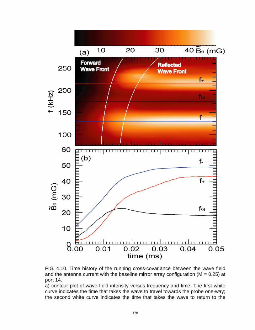
128

FIG. 4.10. Time history of the running cross-covariance between the wave field and the antenna current with the baseline mirror array configuration (M = 0.25) at port 14. a) contour plot of wave field intensity versus frequency and time. The first white curve indicates the time that takes the wave to travel towards the probe one-way; the second white curve indicates the time that takes the wave to return to the

129

probe after being reflected at the anode/cathode the first time. b) Temporal plot of wave field intensity growth at three characteristic frequencies: f+ (215 kHz), f- (130 kHz) and fG (175 kHz).

4.4.6 Continuum Quality Factor Varying with Density

The quality factors of the continuum depend on the damping mechanisms of SAW

propagation, the refraction and reflection at each mirror cell as well as the machine end

condition. Here theoretical damping estimation in a straight field LAPD plasma column

is used as the only contribution to the theoretical quality factor. In Ref. [17], SAW

damping along the ray path through the background field gradient were determined to be

mainly from three mechanisms: the ion-cyclotron damping, the electron Landau damping

and the electron-ion Coulomb collisions. In the baseline mirror array configuration (M =

0.25), the upper continuum f+ is lower than 0.6 fci at B0min, which means that the

ion-cyclotron damping is negligible. For a general resonant mode ω , the theoretical

quality factor can be expressed as:

22

//

)(

+==⊥− ω

ωννω

γω ci

Landaueeie

i

k

k

m

mQ , (4.14)

where eiν is the electron-ion Coulomb collision rate and ων ∝−Landaue is the effective

collision frequency for electron Landau damping rate (see Eq. 4.20). Several spectra are

taken with various ne in the LAPD as shown in FIG. 4.11, where the horizontal axis is the

normalized frequency f / fBragg centered to the upper continuum of each curve. When the

density drops from 2.66 x 1018 m-3 to 1.26 x 1018 m-3, the normalized spectral width drops

as predicted by Eq. 4.14 as shown in the inset. It is also noticeable that the spectral

intensity at the gap center increases with the higher density, which implies that if there

130

are any modes within the gap region, they are not subject to the continuum damping.

More quantitative discussions of mode damping mechanisms will be included in the

simulation works of Sec. 4.5.

FIG. 4.11. Upper continuum spectra width ( ++ f/γ ) with three different plasma densities. The upper continuum of each spectrum is centered at the horizontal origin. The inset shows the normalized spectra width versus plasma density. The error bars as well as the Gaussian fit of the f+ peak are shown for ne = 1.26 x 1018 m-3 case. (All data acquired with 100 MHz sampling rate, averaging 8 samples and 5 consecutive plasma shots. Maximum horizontal error is ± 0.01.)

131

4.5 SAW Spectral Gap Simulation

A linear electro-magnetic wave solver for cold magnetized plasma (Guangye Chen,

Univ. Texas, Austin) is employed to treat a magnetic mirror array configuration. The

details of the solver are described in Ref. [24], in which the solver was used to study

helicon modes.

4.5.1 Electro-Magnetic Wave Solver

The wave field is governed by Maxwell’s equations in the frequency domain

0

1,a

i ,

i

ω

ωµ

∇× = ∇× = − +

E B

B D j (4.15)

where E and B are the electric and magnetic fields, 0µ is the permeability of free space,

D is the electric displacement vector, ω is the antenna frequency, and j a is the antenna

current density. The cold plasma approximation yields the following relation between the

electric displacement vector and the electric field25, 37, ,αβαβαβ ε ED = or equivalently

)))((][(0 bbEbEED ⋅−+×+= εηεε ig (4.16) where b ≡ B0 / B0 is the unit vector along the external magnetic field and

2

2 2

2

2 2

2

1 ,( )

,( )

1 .( )

p

c

pc

c

p

i

i

gi

i

αα

α α α

αα

α α α

α

α α

ωω νεω ω ν ω

ωωω ω ν ω

ωη

ω ω ν

+= − + − = − + − = − +

∑

∑

∑

(4.17)

Here the subscript α labels particle species (electrons and ions), αω p is the plasma

frequency, αωc is the gyro-frequency, and αν is the collision frequency. Singly-ionized

132

helium ions are assumed. Equation (4.15) is solved for a given azimuthal mode number m

on a 2D domain (r, z).

The external magnetic field 0B is axisymmetric, with zr BB 00 << and 00 =θB . It

is therefore appropriate to use a near axis expansion for the magnetic field, which means

that zB0 is treated as a function of z only and

.)(

2

1),( 0

0 z

zBrzrB z

r ∂∂−= (4.18)

The antenna is a blade antenna shown in FIG. 4.2. The components of antenna current

density for the 0=m mode are given by

),()()(2

,0

)],()()[(2

0

0

aaaaaz

a

aaaar

RrzLzHzzHr

Ij

j

LzzzzrHr

Ij

−−+−=

=

−−−−=

δπ

δδπ

θ (4.19)

where 0I is the amplitude of the current, aL is the antenna length, az is the antenna

position as shown in FIG. 4.2, aR is the radius of the horizontal rod, and H is the

Heaviside step function.

4.5.2 Periodic Array of Mirrors

It is convenient to first consider a single mirror cell ( mLz≤≤0 ) with periodic

boundary conditions, which provides an ideal case to study the Bragg reflection induced

spectral gap as well as a benchmark for the realistic simulations of finite number of

mirrors. This single mirror cell has the same sinusoidal profile of the magnetic field

described in Eq. (4.1). The following boundary conditions are used:

1. The chamber wall at r = 0.5 m is assumed to be a conducting boundary where the

tangential components of the electric field vanish;

133

2. Since all the field components are regular at 0→r , there are: 00=

=rBθ and

0)(0=

=rrEθ for 0=m ; 0

0=

=rzE and 0)(0=

=rrEθ for 0≠m ;

3. Periodic boundary condition: 0

( , ) ( , ) s

m

i

z L zeφ

= ==E B E B , where sϕ is the given

phase difference between the field components at 0=z and mLz= .

The experimentally measured radial profile of the plasma density is used in the code

as shown in FIG. 4.3. The density is assumed to be independent of z. The collision

frequency for electrons is calculated as the electron-ion Coulomb collision frequency26

Λ×= −− ln1091.2 2/312eeei Tnν , where eT and en are expressed in eV and m-3,

respectively. The electron temperature is taken to be 8 eV; the Coulomb logarithm is

taken to be Λln = 12. The collision frequency for ions is set to zero.

In this simulation, 8.0=aL m, 1=az m, and 15.0=aR m. Although the antenna

launches several azimuthal modes, the amplitudes of all modes with 0≠m are

significantly smaller than that of the m = 0 mode. Therefore, only m = 0 mode is

considered here.

The amplitude of θB is recorded at (r = 0.04 m , z = 3 m) and normalized by the

antenna current 0I with different values of the phase angle )2,0( πϕ ∈s (FIG. 4.12. a).

In a uniform system, the phase angle sϕ determines the value of zsz Lk /ϕ= . In the

mirror configuration, the forbidden band appears around km = π / Lz . There are two

peaks in θB for each value of sϕ . For various ),0( πϕ ∈s , the lower-frequency peak

represents a right-traveling wave, and the one at the higher frequency is a left-traveling

wave.

134

FIG. 4.12. a): simulation of wave excitation as a function of sϕ and frequency. A sharp forbidden gap of wave excitation is evident between two branches of traveling waves. Here the wave amplitude is normalized by the antenna current. b): the dispersion relation of excited waves from the simulation, in which f corresponds to the maximum of each peak and zsz Lk /ϕ≡ .

At larger values of sϕ ( )2,( ππϕ ∈s ), the waves in both branches change the direction

of propagation, switching from the right to the left in the lower branch, and from the left

to the right in the upper branch. At the transition (where ϕs ≈ π ) the wave becomes a

standing wave, almost fully reflected by the mirrors due to the Bragg reflection. It is clear

that a gap is formed where the wave excitation is significantly suppressed as illustrated

with an envelope (solid line) in FIG. 4.12 (a). The dispersion curves found in the

simulation (FIG. 4.12 b) evidently reproduced FIG. 4.1. More importantly, because of the

definite kz in the simulation, the gap width can be determined accurately at kz = km, which

matches the prediction of Eq. (4.9).

135

4.5.3 Simulation of Mirror Array in the LAPD

Now the mirror array configuration in the LAPD is considered realistically as shown

in FIG. 4.13, with a magnetic beach as an absorbing end and the anode as a reflecting end.

The magnetic beach here is longer (7.74 m) than that in the experiment to ensure

complete absorption of the waves. A finite ion collision frequency iν is introduced to

resolve the ion cyclotron resonance in the beach area. The boundary conditions in the

radial direction remain the same as in the case of infinite periodic system.

FIG. 4.13. Computational setup used to simulate the mirror array in the LAPD shown in FIG. 4.2. a): the computational domain. b): the z component of the external magnetic field (left) and the finite ion collision frequency in the beach area (right).

136

FIG. 4.14. The radial profiles of azimuthal B field (rms) at three frequencies comparing simulation and experimental results. This simulation uses 4=α which is defined in Eq. (4.20).

To be consistent with the experiment, the z coordinates is pointing from right to left;

the origin is set at the left leg of the blade antenna with 0.1=aL m, and 005.0=aR m.

The variable antenna current due to rf coupling efficiency at different frequencies (FIG.

4.6) is used to calculate the wave field amplitude. The radial profile of θB for three

frequencies f = 127 kHz, 167 kHz and 202 kHz is shown in FIG. 4.14, compared with the

experimental measurement at z = 10.25 m (port 14). The calculated quantity θB in the

plot is 2/|),,(| zrfBθ , which is equivalent to the rms average of θB from the

measurement. The frequency scan of the radial maximum value of θB at z = 3.21 m

(port 36) and z = 10.25 m (port 14) are compared with the experimental data in FIG. 4.15.

137

Both in the simulation and the experiment, the wave signal at port 14 exhibits a gap at the

same frequency as in the periodic system, while at port 36, the gap is less obvious

because the detector is only one mirror away from the antenna.

Additional damping mechanism beside electron-ion Coulomb collisions is needed to

match the absolute value of wave amplitude. Since the electron thermal velocity is

comparable to the wave phase velocity in this study, electron Landau damping can play

an important role in the wave propagation. To take into account of the effect of Landau

damping, an effective electron collision frequency is introduced as

v

vte

e LandauA

ων α

−= , (4.20)

where α is a numerical factor. As a result of the frequency dependence of e Landauν−

, the

wave amplitude is more suppressed in the higher frequency region, which makes the

shape of the scan close to that in the experiment. A good agreement of the position, depth

and width of the gap at port 14 is reached in the calculation with α = 4. The

agreement at port 14 is better than that at port 36, which may be due to near-field effects

at port 36.

138

FIG. 4.15. Comparison of θB : experiment versus the simulation.

a): port 14 and b): port 36. The plots show the radial maximum of θB as a function of frequency. Three α values represent possible estimates of effective collision frequencies for Landau damping.

139

With the antenna placed in the last mirror, the waves are launched in both directions. It

is instructive to characterize wave propagation by the wave energy density27

* 2( ' )

4

E EW α β αβω ε

ω ω

∂=

∂ , (4.21)

where 'αβε is the Hermitian part of the dielectric tensor neglecting the collision

frequency. FIG. 4.16 shows the 2-D contour plots of the wave energy density for a

frequency below the forbidden gap at f = 120 kHz, a frequency inside the gap at f = 170

kHz, and a frequency above the gap at f = 220 kHz. It is seen that the wave energy is the

highest at the antenna. For the frequencies away from the forbidden gap, i.e. f = 120 kHz

and 220 kHz, the wave propagates leftwards and reflects as it reaches the boundary, the

anode in the experiment. The magnitude of the wave energy decreases along the

propagation due to damping and absorption. The patterns of wave energy density are

similar at these two frequencies. In the forbidden gap region, e.g. f = 170 kHz, the wave

amplitude decreases faster due to the multiple reflections from the mirror cells. As a result,

the wave energy diminishes as it reaches the anode. On the other hand, for all the cases, the

waves propagate rightwards without much reflection until absorbed at the magnetic beach.

140

FIG. 4.16. The contour plots of wave energy density obtained from Eq. (4.21) for three frequencies. a): f = 120 kHz below the gap; b): f = 170 kHz in the gap; c): f = 220 kHz above the gap.

141

1 Lord Rayleigh, Phil. Msg., vol. 24, pp.145-159; August, (1887).

2 Charles Kittel, Introduction to Solid State Physics, 7th Edition, (John Wiley & Sons Inc., 1996).

3 H. Kogelnik and C. V. Shank, Appl. Phys. Lett. 18 (4), 152 (1971).

4 H. Kogelnik and C. V. Shank, J. Appl. Phys. 43 (5), 2327 (1972).

5 C. K. Chong, D. B. McDermott, M. M. Razeghi, N. C. Luhmann, Jr., J. Pretterebner, D. Wagner, M.

Thumm, M. Caplan, and B. Kulke, IEEE Trans. Plasma Sci., 20 (3), 393 (1992).

6 J. J. Barroso, J. P. L. Neto, and K. G. Kostov, IEEE Trans. Plasma Sci., 31 (4), 752 (2003).

7 E. Yablonovitch, T. J. Gmitter, R. D. Meade, A. M. Rappe, K. D. Brommer, J. D. Joannopoulos,

Phys. Rev. Lett. 67 (24), 3380 (1991).

8 Mehmet Bayindir, B. Temelkuran, and E. Ozbay, Phys. Rev. Lett. 84 (10), 2140 - 2143 (2000).

9 K. F. Casey and J. R. Matthes, J. Math. Phys. 10 (5), 891 (1969).

10 C. Uberoi, Phys. Fluids 15, 1673 (1972).

11 D. A. D’Ippolito and J. P. Goedbloed, Plasma Phys. 22, 1091 (1980).

12 R. L. Dewar et al., Phys. Fluids 17, 930 (1974).

13 R. Betti and J. P. Freidberg, Phys. Fluids B 4, 1465 (1992).

14 M. S. Chu et al., Phys. Fluids B 4, 3713 (1992); Y. I. Kolesnichenko, V. V. Lutsenko, H. Wobig, Y.

V. Yakovenko, O. P. Fesenyuk, Phys. Plasmas 8, 491 (2001).

15 C. Mitchell, S. Vincena, J. Maggs and W. Gekelman, Geophys. Res. Lett., 28 (5), 923 (2001).

16 C. C. Mitchell, J. E. Maggs, and W. Gekelman, Phys. Plasmas 9 (7), 2909 (2002).

17 S. Vincena,a) W. Gekelman, and J. Maggs, Phys. Plasmas 8 (9), 3884 (2001).

18 C. C. Mitchell, J. E. Maggs, S. T. Vincena, and W. N. Gekelman, J. Geophys. Res. 107 (A12), 1469

(2002).

19 M. Abramovitz and I. A. Stegun, Handbook of Mathematical Functions, (Dover Publications, Inc.,

New York, 1972), p 722 (20).

20 H. Boehmer, M. Zales Caponi and J. Munch, in Free Electron Lasers, Proceedings of the 7th Course

142

on Physics and Technology of Free Electron Lasers of the International School of Quantum

Electronics, Erice, 1980, edited by S. Martellucci and Arthur N. Chester .

21 S. Vincena, Ph. D. thesis, Univ. Cal. Los. Angeles, (1999).

22 S. Vincena, W. Gekelman, and J. Maggs, Phys. Rev. Lett. 93 (10), 105003-1(2004).

23 G. Y. Fu and J. W. Van Dam, Phys. Fluids B 1 (10), 1949 (1994).

24 G. Chen, A.V. Arefiev, R.D. Bengtson, B.N. Breizman, C.A. Lee, L.L. Raja, Phys. Plasmas 13,

123507 (2006).

25 T. H. Stix, Waves in Plasmas, (American Institute of Physics, New York, 1992), p. 38.

26 P. Helander and D. J. Sigmar, Collisional Transport in Magnetized Plasmas, (Cambridge University

Press, Cambridge, UK, 2002), p. 5.

27 V.D. Shafranov, Reviews of Plasma Physics 3, (Consultants Bureau, New York, 1967), p. 143.

143

C h a p t e r 5

CHAPTER 5 CONCLUSIONS

5.1 Summary

Two basic plasma experiments are accomplished during this thesis work.

In preparing the hardware for the first experiment, lithium ion sources using lithium –

aluminosilicate as a thermionic emitter were developed and characterized. Two

commercially available emitter sizes (0.6” and 0.25”) with integrated heater assembly

were used. A compact ion gun structure was chosen featuring grids for acceleration –

deceleration sections. In principle, the ion guns can be operated at any angle with respect

to the magnetic field. At high plasma density environment, e. g. the discharge plasma of

the LAPD, a minimum pitch angle must be used to avoid plasma electron loading of the

emitter circuit. Typical ion beam densities are in the 1 mA/cm2 range at beam voltages

between 400 V and 2000 V. The ion guns successfully operated in the discharge of the

LAPD. Collimated/gridded fast-ion analyzers are developed to detect the fast-ion signals

in the LAPD discharge with good signal-to-noise and spatial resolution.

In the first experiment, Doppler shifted cyclotron resonance effect is directly

measured from the beam spatial non-classical spreading caused by single and multi-mode

shear Alfvén waves. Both qualitative and quantitative agreements of the SAW-induced

144

spatial displacements with theory are achieved. Primary and subordinate resonance peaks

in frequency are seen in experiment and simulation. A subordinate resonance is caused by

partial overlapping of the fast ion and wave phases when the frequency is an integer

fraction of the primary frequency. With a pure sine wave drive, a null effect point is

discovered in the resonance spectrum as predicted by theory. This null effect is absent

with a triangle wave drive because higher harmonics cause an extra resonance effect.

Resonance effect is kept within linear regime where spatial displacements are proportional

to SAW amplitude. Both single-particle and Monte-Carlo simulation codes proved robust

for predicting fast-ion resonance experiment. Finally, SAW-induced energy change of fast

ions was verified by variable potential barriers in the fast-ion analyzer.

In the second experiment, the axial magnetic periodicity induced Alfvén spectral gaps

and continua are discovered and characterized experimentally for the first time. The gap

spectral width is found to increase with the Magnetic mirror depth (M), which is predicted

by solving Mathieu’s equation as well as the coupled wave theory in TAE studies1, 2. The

running cross-covariance analysis shows that reflected wave from the LAPD

anode/cathode enhances the features of the spectral gap. The quality factor of the spectral

upper continuum is found to decrease with the plasma density.

A finite-difference simulation code successfully models this experiment in a 2-D r-z

plane. The results from an ideal case with periodic boundary conditions, i.e. infinite

number of mirrors, show wave energy reflection near the frequency satisfying the Bragg

condition. In a realistic simulation using experimental conditions at the LAPD machine,

two candidate damping mechanisms, the electron-ion Coulomb collision and the electron

Landau damping, are both essential in order to match the calculated spectra to the

145

experimental ones.

5.2 Implications

To emphasize the correlation of the second work with the TAE studies, the

similarities between the two are summarized in Table 4, where in both cases a frequency

gap arises due to a periodic modulation of the ambient magnetic field. Due to the toroidal

coupling in a tokamak and the magnetic shear, a certain discrete frequency can exist

inside the gap, i.e. TAE modes.

Experiments Properties TAE SAW in Mirror Array

Periodicity Magnetic field:

B0 (θ) Magnetic field:

B0 (z) Periodic length 2πqR Mirror length: Lm

B0 modulation strength

[Ref. 2]

Wave function ~exp(imθ) ~exp(ik// z)

Bragg Condition k//=n/2qR kn=nπ/Lm

Spectral Gap/ Continuum

Yes Yes

Eigenmodes Yes ?

Table 4 Similarities between TAE and mirror array Alfvén experiment.

In a toroidal geometry, at rational q (safety factor) magnetic surfaces,

where ( ) nmq /2/1+= , two different poloidal modes m and m+1 couple to each other

since their wave vector satisfy

+−= + q

mn

Rkk mm

01////

1. Solving the two coupled

eigenmode equations for poloidal electric fields2, the frequency difference between two

εminmax

minmax

BBBBM +

−=

146

continuum frequency branches is defined as the spectral gap width:

/ /ˆ2 vA mkω ω ω ε+ −∆ = − ≈ . From the analogy in Table 4, with proper substitution of

relevant quantities, the expressions for the spectral gap width in the magnetic mirror array

experiment is 2G Braggf f f Mf+ −∆ = − ≈ . This is shown as the blue dash line in FIG. 4.9.

This work in the LAPD can provide further understanding of the TAE mode due to the

benefits of simplicity and outstanding spatial and temporal resolutions.

5.3 Future work

Several improvements are possible for future experiments. In addition to having a

well-polished emitter surface, a new extraction grid design with less heat expansion can

help maintain the collimation of the fast-ion beam over long operation hours. The fast-ion

signal-to-noise is usually a limit for conducting resonance experiment at large numbers of

gyro-cycles. Coulomb scattering, beam divergence and the intensity loss of the beam to

the plasma make distant observations more difficult. The beam emission current is

usually kept low (< 1 mA) since it is inversely proportional to the source lifetime (~ 20

hrs). The cost of LAPD run time to replace the source on site (~ 6 hr) and the monetary

expense are both significant. A customized lithium-aluminosilicate refilling vacuum

furnace has been designed and tested to be capable of produce glassy emission material

using low-cost raw powder (Heatwave Labs, Inc.). Eventually a 7Li + source containing

two times the emission material (thicker scab) at half the cost would be practical to

operate at much higher emission current. Another way to improve the fast-ion

signal-to-noise is to design a pre-amplifier3, 4 right next to the fast-ion analyzer in order

147

to drive the ~ 10 ft long signal line. This would also enable the analyzer to observe SAW

frequency signal at chosen spatial locations.

An antenna containing two current loops at the correct phase difference can produce

left-circularly polarized SAW. A small gyro-radius (~ 2.5 cm) fast-ion orbit can be

designed to stay in phase and direction with the wave electric field for near a complete

cycle, which further enhances the resonance effect. A smaller footprint of lithium source

is required for this experiment and the existing 0.25” diameter lithium source22 is

suitable.

Fast-ion trapping in the SAW frame requires up to the full length of LAPD plasma.

Orbit designs with fast ions finishing multiple gyro-cycles per port can have the SAW

modified fast-ion energy oscillate faster along the z direction. Then it is convenient to fit

at least one energy oscillating cycle as in FIG. 3.1 b).

Resonance experiments with other types of waves, e.g. electrostatic waves, can also

be considered. Landau resonance experiments with the strong, low pitch angle Ar+ rf

source or the LAPD intense rf fast-ion source are been designed to implement in the near

future.

For UC Irvine fast-ion group, this experiment has established a foundation for

fast-ion transport experiments in turbulence fields. Nonlinear heating of fast-ion beam

with much stronger SAW fields (amplitude δB / B up to 1%) is one adjacent experiment

to try based on L. Chen’s multi-mode heating theory. The natural multi-mode triangular

wave drive can be used to launch SAWs with multiple frequencies and random phases

simultaneously. A conductive, fast-ion gyro-diameter sized disk was inserted into the

LAPD plasma and Alfvén-drift wave turbulence was created downstream (FIG. 5.1).

148

Fast-ion orbit designed to overlap with the strong turbulence fields showed non-classical

transport effects. Further experiments like this will be conducted.

FIG. 5.1. Fast ion transport under turbulence fields experiment in the LAPD plasma. RF source was used in the July 2004 experiment.

It will be further intriguing to study fast-ion transport in modes similar to the TAE

mode in a Tokamak. In order to create eigenmodes in this system, the axial periodicity

has to be broken with a strong defect, which can be made possible by introducing a sector

of magnet with much stronger background field (up to 3.5 kG) compared to the regular

mirror field (FIG. 5.2). The mirror field periods also need to match the reflective

boundary locations at both ends in order to provide the higher Q factor for the possible

modes.

149

FIG. 5.2. Magnetic field with defect in the mirror array in the LAPD. (July 2006 LAPD run)

150

1 G. Y. Fu and J. W. Van Dam, Phys. Fluids B 1 (10), 1949 (1994).

2 H. L. Berk, J. W. Van Dam, Z. Guo, and D. M. Lindberg, Phys. Fluids B 4 (7), 1806 (1992).

3 R. A. Pitts and R. Chavan,S. J. Davies, S. K. Erents, G. Kaveney, G. F. Matthews, G. Neill, J. E.

Vince and JET-EFDA workprogramme contributors, Rev. Sci. Instr. 74 (11), 4644 (2003)

4 P. Pribyl, W. Gekelman, M. Nakamoto, E. Lawrence, F. Chiang, J. Stillman, J. Judy, N. Katz, P.

Kintner, P. Niknejadi, Rev. Sci. Instr. 77, 073504 (2006)

151

APPENDIX A: Typical Ion Beam and the LAPD Plasma Parameters

I. The LAPD plasma (Helium plasma)

Magnetic field, B 1.0 -2.0 kG

Pressure, P 52.3 10 Torr−×

Electron density in afterglow, en 11 310 cm−

Electron density in Discharge, en 12 32 10 cm−×

Neutral density, 0n 11 36 10 cm−×

Electron temperature in afterglow, eT 0.13 eV

Electron temperature in Discharge, eT 6 - 7 eV

Ion temperature in afterglow,iT 0.1 eV

Ion temperature in Discharge,iT 1 eV

Plasma column length 18 m

Plasma column diameter 70 cm

Cathode-anode discharge current 5 - 6 kA

Cathode-anode discharge frequency 1 Hz

Afterglow time 50-60 ms

Discharge time 8 - 10 ms

Floating potential 45-50 V

152

II. Fast-ion beam (argon beam) and ion gun

Beam energy, W ~ 600 eV

Beam current density, j 1 2/mA cm

Beam size 0.5 cm Dia.

Pitch angle,θ 28 - 50º

Gyro-radius of fast ions,ρ 3 - 6 cm

Emitter voltage 600V

Accelerator voltage - 100 V

Energy spread,E∆ ~15 eV

Beam divergence ~5 degrees

153

APPENDIX B: Important Data Sets Supporting Experimental Results

In the LAPD backup folder (usually two copies on the lab computers), a data run

between July 2004 and Dec 2007 can be found in “PLASMA\Fast Ion

Turbulence\UCLA\”. Each data run has a separate folder with the month or the first day

of the experiment to be the folder name. A master experiment log is in MS Excel format

and named “Exp log 5.9.2005”, for example, which contains the details of the data sets

taken during that run. If the data set contains hdf5 copies, then it is convenient to use an

IDL program called “read_parameters.pro” to load the experimental setups for each data

set. Important data set names and corresponding programs related to the results shown in

this thesis is listed as follows.

I . Fast Ion Doppler Resonance Experiment

Programs can be found in PLASMA\Fast Ion Turbulence\UCLA\\LAPDdata\9.11.2007FIAR\FIAR.prj

Figure Data Set(s) IDL programs

FIG. 3.1 Fig1_FIAR_bdata.dat saw_init_59mm.pro

derivs_alfven_59mm.pro

PLASMA\Fast Ion

Turbulence\simulation\single particle alfven motion

lorentz_saw_59mm.pro

Fig1_FIAR.pro

FIG.3.2 jan20_0.1_0.8_0.005wci_norec_40ports.dat

Fig2_FIAR_a.pro

jan28_0.1_0.8_0.005wci_norec_3ports.d

at fig2b_FIAR.pro

jan28_0.1_0.8_0.005wci_norec_10ports.

dat

feb12_0.1_0.8_0.005wci_norec_3ports_1

0G.dat

PLASMA\Fast Ion

Turbulence\simulation\single particle

154

alfven motion

FIG.3.4 orbit_MC 0.650000Feb140G.dat DSC_FIAR.pro

orbit_MC 0.650000Jan25.2008.dat orbits_SAW.pro

orbit_MC 0.200000Feb1510G.dat Fig_4_FIAR.pro

PLASMA\Fast Ion

Turbulence\simulation\Monte_Carlo_SAW

FIG.3.7 10th_HYBIII_p32_sine_95kHz. SIS 3301 .dat

Fig_active_beam_profile_FIAR.pro

10th_HYBIII_p32_sine_95kHz.hdf5

(Use only the no SAW data)

\LAPDdata\12.04.2007FIAR

FIG.3.8 6th_b6_p33_50V_297kHz.SIS 3301.dat Fig88_FIAR.pro

\LAPDdata\12.04.2007FIAR

FIG.3.9 16th_b9_p36_fscan_50-500_10kHz_1200Gflare_80V. SIS 3301.dat Fig7b_rms_FIAR.pro

\LAPDdata\9.11.2007FIAR (7b is old label)

FIG.3.10 \LAPDdata\9.11.2007FIAR\16th_b9_p36_plane_fscan_80V. SIS 3301.dat Fig10_FIAR.pro

\LAPDdata\12.04.2007FIAR\10th_b6_p33_SAW_8f. SIS 3301.dat

\LAPDdata\9.11.2007FIAR\17th_b10_p31_plane_fscan_80V. SIS 3301.dat

FIG.3.11 \LAPDdata\12.04.2007FIAR\9th_HYBIII_p32_SAW_8f. SIS 3301.dat FIG_RC_SAW.pro

FIG_RC_SAW_plot.pro

FIG.3.12 \LAPDdata\9.11.2007FIAR\16th_FIAR_HYBIII_297kHz_80V. SIS 3301.dat rdsaw10shots_911_saveallshots.pro

Fig12_FIAR.pro

Fig12a_FIAR.pro

Fig12bc_FIAR.pro

read_saw_1s_6chn_911.pro

FIG.3.13 \LAPDdata\9.11.2007FIAR\16th_FIAR_HYBIII_297kHz_80V. SIS 3301.dat Fig13a_FIAR.pro

Fig13bc_FIAR.pro

Fig13bc_FIAR_plot.pro

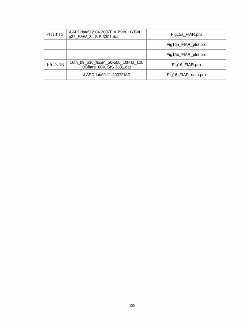
155

FIG.3.15 \LAPDdata\12.04.2007FIAR\9th_HYBIII_p32_SAW_8f. SIS 3301.dat Fig15a_FIAR.pro

Fig15a_FIAR_plot.pro

Fig15b_FIAR_plot.pro

FIG.3.16 16th_b9_p36_fscan_50-500_10kHz_1200Gflare_80V. SIS 3301.dat Fig16_FIAR.pro

\LAPDdata\9.11.2007FIAR Fig16_FIAR_data.pro

156

II . SAW Spectra Gap in the LAPD Mirror Array

Programs can be found in PLASMA\Fast Ion Turbulence\UCLA\1.25.2007 MAE\data \MAE2007Jan.prj

Figure Data Set(s) IDL programs

FIG. 4.3 triple_jan27_p13f_m1200base_13ne. SIS 3301.dat

Figure_2_plasma.pro

triple_jan26_p19m_m1200base_13ne_c.

SIS 3301.dat

triple_jan27_p35m_m1200base_13ne.

SIS 3301.dat

PLASMA\Fast Ion

Turbulence\UCLA\1.25.2007 MAE\data

FIG. 4.4 Jan26th_p14_no6_fscan_m1200_rod_13ne. SIS 3301.dat

Figure_b_vs_r.pro

Figure_rb2_vs_r.pro

FIG. 4.6 Jan26th_p14_no6_fscan_m1200_rod_13ne. SIS 3301.dat

Figure_5_U_character.pro

PLASMA\Fast Ion

Turbulence\UCLA\1.25.2007 MAE\data Fig5_iant.pro

Jan26th_p14_no6_fscan_m1200_rod_13

ne

FIG. 4.8 Jan26th_p14_no6_fscan_m1200_rod_13ne

Fig7a.pro

p14_p36_m1200deep_10ne Fig7a_flat.pro

p14_p36_m1200shal25percent_13ne Fig7b_disk.pro

Jan25th_p14_no6_fscan_flat1200_rod

PLASMA\Fast Ion

Turbulence\UCLA\1.25.2007 MAE\data

FIG. 4.10 Jan26th_p14_no6_fscan_m1200_rod_13ne. SIS 3301.dat Fig9.pro

PLASMA\Fast Ion Turbulence\UCLA\1.25.2007 MAE\data running_ccov.pro

157

APPENDIX C: Schematics for Experimental Apparatuses

I. 0.6” dia. Emitter Lithium Fast-ion Source (LiGun)

FIG. 0.1 Photograph (left) and inside structure (right) of the 0.6” emitter lithium source (LiGun).

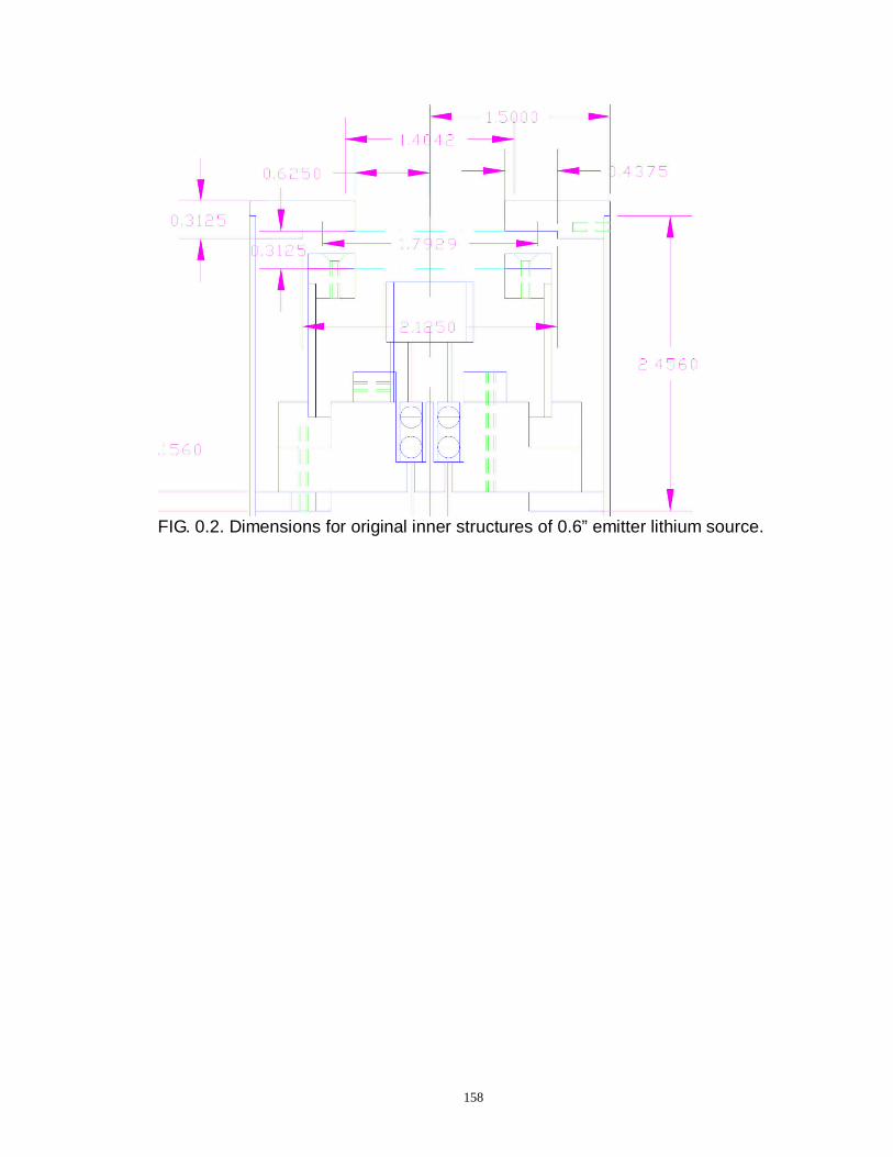
158

FIG. 0.2. Dimensions for original inner structures of 0.6” emitter lithium source.

159

FIG. 0.3. Modified grid structure of 0.6” emitter lithium source showing 28º of incident angle to the edge of the emitter, with 0.5 cm diameter aperture.

160

II. 0.25” dia. Emitter Lithium Fast-ion Source (mini-Li Gun)

161

III. Lithium Source High Voltage Power Supply Schematics

162

IV. Lithium Source Re-coating Device Schematics

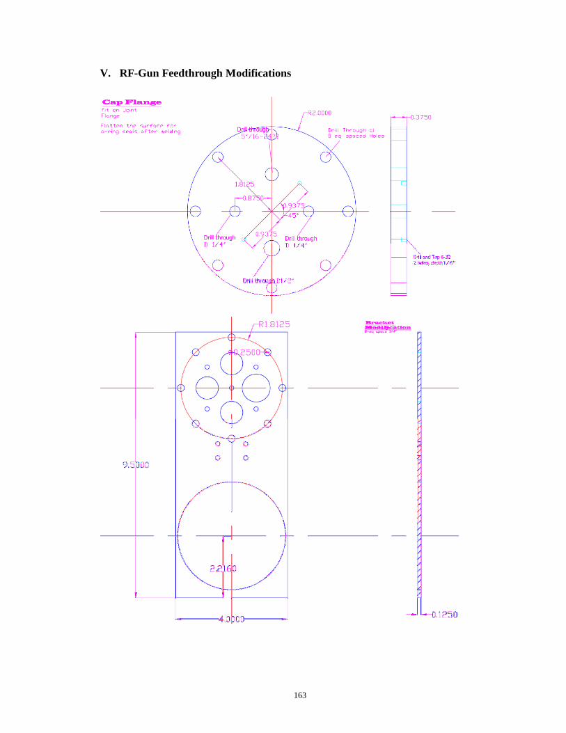
163

V. RF-Gun Feedthrough Modifications

164

APPENDIX D: Instrument Calibration Data

I. Calibration of b-dot probes at the LAPD

Fast Ions and Shear Alfvén Waves - UCI Physics and Astronomy

Documents

Transcript of Fast Ions and Shear Alfvén Waves - UCI Physics and Astronomy