Fast Incremental Maintenance of Approximate...

Fast Incremental Maintenance ofApproximate Histograms

PHILLIP B. GIBBONSIntel Research PittsburghYOSSI MATIASTel Aviv UniversityandVISWANATH POOSALABell Laboratories

Many commercial database systems maintain histograms to summarize the contents of large re-lations and permit efficient estimation of query result sizes for use in query optimizers. Delayingthe propagation of database updates to the histogram often introduces errors into the estima-tion. This article presents new sampling-based approaches for incremental maintenance of ap-proximate histograms. By scheduling updates to the histogram based on the updates to thedatabase, our techniques are the first to maintain histograms effectively up to date at all times andavoid computing overheads when unnecessary. Our techniques provide highly accurate approxi-mate histograms belonging to the equidepth and Compressed classes. Experimental results showthat our new approaches provide orders of magnitude more accurate estimation than previousapproaches.

An important aspect employed by these new approaches is a backing sample, an up-to-daterandom sample of the tuples currently in a relation. We provide efficient solutions for maintaininga uniformly random sample of a relation in the presence of updates to the relation. The backingsample techniques can be used for any other application that relies on random samples of data.

Categories and Subject Descriptors: H.2.4 [Database Management]: Systems—query processing

General Terms: Algorithms, Experimentation, Performance

Additional Key Words and Phrases: Approximation, histograms, incremental maintenance, sam-pling, query optimization

This work was performed while all three authors were with the Information Sciences ResearchCenter, Bell Laboratories.A preliminary version of this article appeared in Proceedings of the 23rd International Conferenceon Very Large Data Bases (Athens, August), 1997, pp. 466–475.Authors’ addresses: P. B. Gibbons, Intel Research Pittsburgh, 417 South Craig Street, Suite 300,Pittsburgh, PA 15213; email: [email protected]; Y. Matias, Department of Computer Sci-ence, Tel Aviv University, Tel Aviv 69978, Israel; email: [email protected]; V. Poosala, Bell Lab-oratories, Room 2A-212, 600 Mountain Avenue, Murray Hill, NJ 07974; email: [email protected] to make digital/hard copy of part or all of this work for personal or classroom use isgranted without fee provided that the copies are not made or distributed for profit or commercialadvantage, the copyright notice, the title of the publication, and its date appear, and notice is giventhat copying is by permission of the ACM, Inc. To copy otherwise, to republish, to post on servers,or to redistribute to lists, requires prior specific permission and/or a fee.C© 2002 ACM 0362-5915/02/0900-0261 $5.00

ACM Transactions on Database Systems, Vol. 27, No. 3, September 2002, Pages 261–298.

262 • P. B. Gibbons et al.

1. INTRODUCTION

Most database management systems (DBMSs) maintain a variety of statisticson the contents of the database relations in order to estimate various quanti-ties, such as selectivities within cost-based query optimizers. These statisticsare typically used to approximate the distribution of data in the attributesof various database relations. It has been established that the validity of theoptimizer’s decisions may be critically affected by the quality of these approx-imations [Christodoulakis 1984; Ioannidis and Christodoulakis 1991]. This isbecoming particularly evident in the context of increasingly complex queries(e.g., data analysis queries).

The most common technique used in practice for selectivity estimation ismaintaining histograms on the frequency distribution of an attribute. A his-togram groups attribute values into “buckets” (subsets) and approximates trueattribute values and their frequencies based on summary statistics maintainedin each bucket [Kooi 1980]. For most real-world databases, there exist his-tograms that produce low error estimates while occupying reasonably smallspace (of the order of 1 K bytes in a catalogue) [Poosala 1997]. Histograms areused in IBM DB2, Informix, Ingres, Oracle, Microsoft SQL Server, Sybase, andTeradata. They are also being used in other areas, for example, parallel joinload balancing [Poosala and Ioannidis 1996] to provide various estimates.

Histograms are usually precomputed on the underlying data and used with-out much additional overhead inside the query optimizer. A drawback of usingprecomputed histograms is that they may become outdated when the data in thedatabase are modified, and hence introduce significant errors in estimations.On the other hand, it is clearly impractical to compute a new histogram afterevery update to the database. Fortunately, it is not necessary to keep the his-tograms perfectly up to date at all times, because they are used only to providereasonably accurate estimates (typically within 1 to 10%). Instead, one needsappropriate schedules and algorithms for propagating updates to histograms,so that the database performance is not affected.

Despite the popularity of histograms, issues related to their maintenancehave only recently started receiving attention. Most of the work on histogramsso far has focused on proper bucketizations of values in order to enhance theaccuracy of histograms, and assumed that the database is not being modified.In our earlier work, we have introduced several classes of histograms that of-fer high accuracy for various estimation problems [Poosala et al. 1996]. Wehave also provided efficient sampling-based methods to construct various his-tograms, but ignored the problem of maintaining histograms. In a more generalcontext, we can view histograms as materialized views, but they are differentin certain aspects. First, during utilization, they are typically maintained inmain memory, which implies more constraints on space. Second, they need tobe maintained only approximately, and can therefore be considered as cachedapproximate materialized views. We are not aware of any prior work on approx-imate materialized views.

The most common approach used to date for histogram updates, which is fol-lowed in nearly all commercial systems, is to recompute histograms periodically

ACM Transactions on Database Systems, Vol. 27, No. 3, September 2002.

Maintenance of Approximate Histograms • 263

(e.g., every night or on demand). This approach has two disadvantages: anysignificant updates to the data between two recomputations could cause poorestimations in the optimizer, and recomputing a histogram from scratch byscanning the entire relation is computationally expensive for large relations.

In this article, we present fast and effective procedures for maintainingtwo histogram classes used extensively in database management systems:equidepth histograms (which are used in most DBMSs) and Compressed his-tograms (used in DB2). There are several key novel components to our approach.

(1) We introduce the notion of an approximate histogram that is maintainedin the presence of database updates, and which provides bounds on itsmaximum deviation from the true histogram.

(2) We develop a split and merge technique for quickly adjusting histogrambuckets in response to data updates.

(3) We introduce the notion of a “backing sample,” a random sample of the datathat is kept up to date in the presence of database updates. We demonstrateimportant advantages gained by using a backing sample when updatinghistograms, and present algorithms for its maintenance. We observe thatthe backing sample can be used in any application that requires uniformrandom samples of the current data in the database. For example, insteadof dynamically computing samples at usage-time (which is a drawback ofseveral sampling-based techniques), one can precompute the samples anduse our techniques to maintain them efficiently.1

The main advantages of our techniques are as follows.

— Our approach leads to approximate histograms that are close to the actualhistogram belonging to the same class, with high probability, regardless ofthe data distribution.

— Our algorithms handle all forms of updates to the database (insert, delete, andmodify operations). They are most efficient in insert-intensive environmentsor in data warehousing environments that house transactional informationfor sliding time windows.

— Our algorithms process the sequence of database updates; they almost neveraccess the relation on disk (the only exception is when the size of the relationhas shrunk dramatically due to deleting, say, half the tuples). For most insertoperations, our algorithms do not access the backing sample. The samplenevertheless remains up to date at all times.

We conducted an extensive set of experiments studying our techniquesand comparing them with the traditional approaches based on recomputation.The experiments confirm the theoretical findings and show that with a smallamount of additional storage and CPU resources, our techniques maintain his-tograms nearly up to date at all times.

1If a sampling-based algorithm requires a sample that may be larger than what is maintained,as can be the case for adaptive sampling [Lipton et al. 1990], then some ad hoc sampling may beunavoidable.



Recent Work. Since the completion of our work discussed in this article,there have been a number of important developments in the area of histogrammaintenance and related topics. First, there has been some commercial ac-ceptance of using sampling to speed up histogram recomputation. For exam-ple, when SQL Server recomputes a histogram, it first extracts a randomsample from the relation and then computes the histogram from the sample(see Chaudhuri et al. [1998]). Thus the extracted random sample serves thesame function as a backing sample, for the restricted purpose of computing anew histogram from scratch. Sampling during recomputation has the advan-tage that there are no overheads at database update time (versus the minimaloverheads with backing samples). On the other hand, as discussed in Section 3and elsewhere in this article, there are a number of advantages to having a pre-computed and maintained backing sample, and we exploit these advantages inour algorithms.

Second, a split and merge approach has been used to incrementally main-tain histograms in response to feedback from the query execution engine aboutthe actual selectivities of range queries [Aboulnaga and Chaudhuri 1999]. Suchhistograms are called self-tuning histograms, because they automatically adaptto changes in the database without looking at the updates and without re-computing from the database. Instead, the actual selectivity of the executedrange query is compared with the histogram estimate of that selectivity, andthe histogram bucket counts are adjusted by spreading any discrepancy overthe buckets that lie within the query range. Buckets with large counts are split.Buckets of near-equal frequencies are merged. Since a backing sample (or anyequivalent means) is not used, there are no bounds proved for the maximum de-viation of a self-tuning histogram from the true histogram. On the other hand,experimental results reported by Aboulnaga and Chaudhuri [1999] showed thetechnique performs well for multidimensional data distributions with low tomoderate skew. More recently, Bruno et al. [2001] applied a similar feedback-based technique to multidimensional histograms. A key feature of their ap-proach is its flexible partitioning of the multidimensional space into buckets.Unlike the techniques presented in our article, neither of these approaches usesthe contents of the data in a direct manner.

Finally, there have been a number of recent papers on approximate his-tograms, their maintenance, and their use in query result size estimation andin providing fast approximate answers to queries (e.g., Blohsfeld et al. [1999],Deshpande et al. [2001], Gilbert et al. [2002a,b], Greenwald and Khanna [2001],Gunopulos et al. [2001], Guha et al. [2001], Ioannidis and Poosala [1999],Jagdish et al. [1998], Konig and Weikum [1999], Matia et al. [1998, 2000], andPoosala and Ioannidis [1997]). Moreover, the notion of a backing sample hasbeen extended to the general notion of precomputed (and maintained) sampling-based data synopses, which have been shown to be effective for providing fast ap-proximate answers to queries (c.f. Acharya et al. [2000, 1999], Chaudhuri et al.[2001], Ganti et al. [2000], Gibbons [2001], and Gibbons and Matias [1998]).

Outline of the Article. In Section 2, we discuss histograms, approximate his-tograms, and histogram maintenance. Backing samples and their maintenance



are described in Section 3. Sections 4 and 5 present our algorithms for incre-mental maintenance of approximate equidepth histograms and Compressedhistograms, respectively. Our experimental evaluation is in Section 6, followedby conclusions in Section 7. A number of the proofs are left to the appendix.

2. HISTOGRAMS AND THEIR MAINTENANCE

The domain D of an attribute X is the set of all possible values of X and thevalue set V (⊆ D) for a relation R is the set of values of X that are presentin R. Let V ={vi : 1≤ i≤ |V|}, where vi < vj when i< j and |V| is the cardinal-ity of the set V. The frequency fi of vi is the number of tuples in R whosevalue for attribute X is vi. The data distribution of X (in R) is the set of pairsT ={(v1, f1), (v2, f2), . . . , (v|V|, f |V|)}.

A histogram on attribute X is constructed by partitioning the data distribu-tion T into β (≥1) mutually disjoint subsets called buckets and approximatingthe values and frequencies in each bucket in some common fashion. Typically,a bucket is assumed to contain either all m values in D between the smallestand largest values in that bucket (the bucket’s range), or just k≤m equidistantvalues in the range, where k is the number of distinct values in the bucket. Theformer is known as the continuous value assumption [Selinger et al. 1979], andthe latter is known as the uniform spread assumption [Poosala et al. 1996]. Letthe bucket frequency f B be the number of tuples in R whose value for attributeX is in bucket B.2 The frequencies for values in a bucket B are approximatedby their averages, that is, by either f B/m or f B/k.

Different classes of histograms can be obtained by using different rulesfor partitioning values into buckets. In this article, we focus on two impor-tant classes of histograms, namely, the equidepth and Compressed(V, F) (sim-ply called Compressed in this article) classes. In an equidepth (or equiheight)histogram, contiguous ranges of attribute values are grouped into bucketssuch that the number of tuples f B in each bucket B is the same. In a Com-pressed(V, F) histogram [Poosala et al. 1996], the n highest frequencies arestored separately in n singleton buckets; the rest are partitioned as in anequidepth histogram. In our target Compressed histogram, the value of nadapts to the data distribution to ensure that no singleton bucket can fit withinan equidepth bucket and yet no single value spans an equidepth bucket. Wehave shown in our earlier work [Poosala et al. 1996] that Compressed his-tograms are very effective in approximating distributions of low or high skew.

Equidepth histograms are used in one form or another in nearly all commer-cial systems, except DB2 which uses the more accurate Compressed histograms.

Histogram Storage and Usage. For both equidepth and Compressed his-tograms, we store for each bucket B the largest value in the bucket, B.maxval,

2For any value v that is the right endpoint of ranges for k ≥ 1 buckets, Bi , Bi+1, . . . , Bi+k−1, there isambiguity as to how to divide its frequency fv in the entire relation among f Bi , f Bi+1 , . . . , f Bi+k . Inthis article, we select the following resolution to this ambiguity. If fv > (k− 1)N/β, we assign N/βof fv to each bucket Bj , j = i + 1, . . . , i + k − 1, with v for both endpoints, so that f Bj =N/β. Theremainder of fv is assigned to f Bi ; none is assigned to f Bi+k . If fv ≤ (k− 1)N/β, we assign f Bi = 1,f Bi+k = 0, and, for j = i + 1, . . . , i + k− 1, f Bj = ( fv − 1)/(k− 1).



and a count, B.count, that equals or approximates f B. If B is a singleton bucket,then its range is the single value B.maxval. Otherwise, its range is from theB′.maxval of its preceding bucket (or the minimum value in the domain D, ifB is the first bucket) to B.maxval, excluding the value of each singleton bucketwithin this range (if any).

When using the histograms to estimate range selectivities, we use the ex-act range information provided by singleton buckets and apply the continuousvalue assumption for equidepth buckets. For equidepth buckets, the uniform-spread assumption could be used instead, but it requires knowing the numberof distinct values in each bucket, which is challenging to maintain (even ap-proximately) under updates both to the database and to the histogram bucketboundaries.

2.1 Approximate Histograms

An approximate class C histogram H∗ on an attribute X for a relation R isa histogram that may deviate from the actual class C histogram H as R isupdated. This deviation occurs because we cannot afford to recompute H eachtime R is updated. As R is modified, H∗ may deviate from H in the followingways.

(1) Class Error: H∗ may no longer be the correct class C histogram for R; forexample, it may not have the same bucket boundaries as H.

(2) Distribution Error: H∗ may contain inaccurate information about X ; forexample, it may not have the same bucket counts as H.

The quality of an approximate histogram can be evaluated according to variouserror metrics defined based on the class and distribution errors.

The µcount Error Metric. As an example, consider the following distributionerror metric, relevant to many histogram classes, which reflects the accuracy ofthe counts associated with each bucket. When R is modified, but the histogramis not, then there may be buckets B with B.count 6= f B; the difference betweenf B and B.count is the approximation error for B. We consider the error metricµcount defined as:

µcount= β

N

√√√√1β

β∑i=1

( f Bi − Bi.count)2 , (1)

where N is the number of tuples in R and β is the number of buckets. This isthe standard deviation of the bucket counts from the actual number of elementsin each bucket, normalized with respect to the mean bucket count (N/β).

2.2 Incremental Histogram Maintenance

The approach followed for maintenance in nearly all commercial systems is torecompute histograms periodically (e.g., every night), regardless of the numberof updates performed on the database. This approach has two disadvantages:any significant updates to the data since the last recomputation could result in



Fig. 1. Typical sizes of various entities.

poor estimations by the optimizer, and because the histograms are recomputedfrom scratch by discarding the old histograms, the recomputation phase forthe entire database can be computationally very intensive and may have to beperformed when the system is lightly loaded or offline.3

Instead, we propose an incremental technique, which maintains approxi-mate histograms within specified error bounds at all times with high proba-bility and never accesses the underlying relations for this purpose. There aretwo components to our incremental approach: maintaining a backing sample;and a framework for maintaining an approximate histogram that performs afew program instructions in response to each update to the database,4 and de-tects when the histogram is in need of an adjustment of one or more of itsbucket boundaries. Such adjustments make use of the backing sample. Thereis a fundamental distinction between the backing sample and the histogram itsupports: the histogram is accessed far more frequently than the sample anduses less memory, and hence it can be stored in main memory whereas thesample is likely stored on disk. Figure 1 shows typical sizes of various entitiesrelevant to our discussion.

Incremental histogram maintenance was previously studied in Gibbons andMatias [1998] for the important case of a high-biased histogram, which is aCompressed histogram with β − 1 buckets devoted to the β − 1 most frequentvalues, and 1 bucket devoted to all the remaining values. This algorithm didnot use the approach described above—for example, no backing sample wasmaintained or used.

In the next section, we describe how the backing sample is maintained inthe context of our approach.

3. BACKING SAMPLE

A backing sample is a uniform random sample of the tuples in a relation thatis kept up to date in the presence of updates to the relation. For each tuple, thesample contains the unique row id and one or more attribute values.

3To help alleviate this latter problem, some commercial systems such as SQL Server recompute (ap-proximate) histograms by first sampling the data and then computing a histogram on the sampleddata (as discussed in Section 1).4To further reduce the overhead of our approach, the few program instructions can be performedonly for a random sample of the database updates (as discussed in Section 6.2).



We argue that maintaining a backing sample is useful for histogram com-putation, selectivity estimation, and so on. In most sampling-based estimationtechniques, whenever a sample of size n is needed, either the entire relationis scanned to extract the sample, or several random disk blocks are read. Inthe latter case, the tuples in a disk block may be highly correlated, and henceto obtain a truly random sample, n disk blocks must be read. In contrast, abacking sample can be stored in consecutive disk blocks, and can therefore bescanned by reading sequential disk blocks. Moreover, for each tuple in the sam-ple, only the unique row id and the attribute(s) of interest are retained. Thusthe entire sample can be stored in only a small number of disk blocks, for evenfaster retrieval. Finally, an indexing structure for the sample can be created,maintained, and stored; the index enables quick access to sample values withinany desired range.

At any given time, the backing sample for a relation R needs to be equivalentto a random sample of the same size that would be extracted from R at thattime. Thus the sample must be updated to reflect any updates to R, but withoutthe overheads of such costly extractions. In this section, we present techniquesfor maintaining a provably random backing sample of R based on the sequenceof updates to R, while accessing R very infrequently (R is accessed only whenan update sequence deletes about half the tuples in R).

Let S be a backing sample maintained for a relation R. We first considerinsertions to R. Our technique for maintaining S as a simple random samplein the presence of inserts is based on the Reservoir Sampling techniques dueto Vitter [1985]. Typically, in DBMSs, the reservoir sampling algorithm is usedto obtain a sample of the data during a single scan of the relation without apriori knowledge about the number of tuples in the relation. The particularversion described here (called Algorithm X in Vitter’s paper), is as follows. Thealgorithm proceeds by inserting the first n tuples into a “reservoir.” Then arandom number of records are skipped, and the next tuple replaces a randomlyselected tuple in the reservoir. Another random number of records are thenskipped, and so forth, until the last record has been scanned. The distributionfunction of the length of each random skip depends explicitly on the numberof tuples scanned so far, and is chosen such that each tuple in the relation isequally likely to be in the reservoir after the last tuple has been scanned. Bytreating the tuple being inserted in the relation as the next tuple in the scanof the relation, we essentially obtain a sample of the data in the presence ofinsertions.

Extensions to Handle Modify and Delete Operations. We extend Vitter’s al-gorithm to handle modify and delete operations, as follows. Modify operationsare handled by updating the value field, if the tuple is in the sample. Deleteoperations are handled by removing the tuple from the sample, if it is in thesample. However, such deletions decrease the size of the sample from the targetsize n and, moreover, it is not known how to use subsequent insertions to obtaina provably random sample of size n once the sample has dropped below n. In-stead, we maintain a sample whose size is initially a prespecified upper boundU , and allow for it to decrease as a result of deletions of sample items down



MaintainBackingSample()

// S is the backing sample, R is the relation, X is the attribute of interest.// L and U are prespecified lower and upper bounds for the size of the sample.

After an insert of a tuple τ with τ.I D= id and τ.X = v into R:if |S| + 1= |R| ≤U then

S := S + {(id , v)};else with probability |S|/|R| do begin

select a tuple (id ′, v′) in S uniformly at random;S := S + {(id , v)}− {(id ′, v′)};

end;

After a modify to a tuple τ with τ.I D= id in R:if the modify changes τ.X then do begin

if id is in S thenupdate the value field for tuple id in S;

end;

After a delete of a tuple τ with τ.I D= id from R:if id is in S then do begin

remove the tuple id from S;

// This next conditional is expected to be true only when a constant// fraction of the database updates are delete operations.if |S| < min(|R|, L) then do begin

// Discard S and rescan R to compute a new S.S := ∅;rescan R, and for each tuple, apply the above procedure for inserts into R;

end;end;

Fig. 2. An algorithm for maintaining a backing sample of a relation under updates to the database.

to a prespecified lower bound L. If the sample size drops below L, we rescanthe relation to repopulate the random sample. In the appendix, we show thatsuch rescans are expected to be infrequent for large relations and, moreover,for databases with infrequent deletions, no such rescans are expected. Evenin the worst case where deletions are frequent, the cost of any rescans can beamortized against the cost of the (expected) large number of deletions requiredbefore a rescan becomes necessary.

Our algorithm, denoted MaintainBackingSample, is depicted in Figure 2.For each tuple selected for the backing sample S, we store its (unique) row idand the value(s) of all attribute(s) of interest to any applications that will usethe backing sample (e.g., for histograms, we store the value of the attributeon which the histogram is to be computed). For simplicity, we have shown inthis figure only the case of a single attribute, X , of interest, and we have notshown any of the performance optimizations described below. The algorithmmaintains the property that S is a uniform random sample of a relation R suchthat min(|R|, L)≤ |S| ≤U .

THEOREM 3.1. Algorithm MaintainBackingSample maintains a uniformrandom sample of relation R.

The proof appears in the appendix.



Optimizations. There are several techniques that can be applied to lowerthe overheads of the algorithm. First, a hash table of the row ids of the tuplesin S can be used to speed up the test of whether an id is in S. Second, if the pri-mary source of delete operations is to delete from R all tuples before a certaindate, as in the case of many data warehousing environments that maintain asliding window of the most recent transactional data on disk, then such deletescan be processed in one step by simply removing all tuples in S that are beforethe target date. Third, and perhaps most importantly, we observe that the al-gorithm maintains a random sample independent of the order of the updatesto the database. Thus we can “rearrange” the order to suit our needs, until anup-to-date sample is required by the application using the sample. We can uselazy processing of modify and delete operations, whereby such operations aresimply placed in a buffer to be processed as a batch whenever the buffer becomesfull or an up-to-date sample is needed. Likewise, we can postpone the process-ing of modify and delete operations until the next insert that is selected for S.Specifically, instead of flipping a biased coin for each insert, we select a ran-dom number of inserts to skip, according to the criterion of Vitter’s AlgorithmX (this criterion is statistically equivalent to flipping the biased coin each in-sert). At that insert, we first process all modify and delete operations that haveoccurred since the last selected insert; then we have the new insert replacea randomly selected tuple in S. Another random number of inserts are thenskipped, and so forth. Note that postponing the modify and delete operationsis important, since it reduces the problem to the insert-only case, and hencethe criterion of Algorithm X can be applied to determine how many inserts toskip.

With these optimizations, insert and modify operations to attributes not ofinterest are processed with minimal overhead, whereas delete and modify op-erations to attributes of interest may require larger overhead (due to the batchprocessing of testing whether the id is in the sample). Thus the algorithm is bestsuited for insert-mostly databases or for the data warehousing environmentsdiscussed above.

4. FAST MAINTENANCE OF APPROXIMATE EQUIDEPTH HISTOGRAMS

In this section, we demonstrate our approach for incremental histogram main-tenance by considering a specific important histogram: the equidepth his-togram. First, we present an algorithm for maintaining an approximate equi-depth histogram in the presence of insertions to the database; this algorithmhas provable guarantees on its accuracy. Next, we show how heuristics can beused to modify the algorithm in order to minimize the overheads. Finally, weshow how to extend both algorithms to handle modify and delete operations tothe database. We assume throughout that a backing sample S is being main-tained using the algorithm of Figure 2.

The standard algorithm for constructing an (exact) equidepth histogramfirst sorts the tuples in the relation by attribute value, and then selects tu-ples bi · N/βc, for i= 1, . . . , β. However, for large relations, this algorithm isquite slow because the sorting may involve multiple I/O scans of the relation.



EquiDepthSampleCompute();

// S is the sample to be used to compute the histogram, sorted on the attribute value X .// N is the total number of tuples in R.// β is the desired number of buckets.

For i := 1 to β do beginτ := the bi · |S|/βc’th tuple in S;Bi .maxval := τ.X ;Bi .count := bi · N/βc − b(i − 1) · N/βc;

end;

return ({B1, B2, . . . , Bβ })Fig. 3. Procedure for computing an approximate equidepth histogram from a random sample.

An approximate equidepth histogram approximates the exact histogram byrelaxing the requirement on the number of tuples in a bucket and/or the accu-racy of the counts. Such histograms can be evaluated based on how close thebuckets are to N/β tuples and how close the counts are to the actual numberof tuples in their respective buckets.

A Class Error Metric for Equidepth Histograms. Consider an approximateequidepth histogram with β buckets for a relation of N tuples. We consideran error metric µed that reflects the extent to which the histogram’s bucketboundaries succeed in evenly dividing the tuples in the relation:

µed = β

N

√√√√1β

β∑i=1

(f Bi −

Nβ

)2

. (2)

This is the standard deviation of the buckets’ sizes from the mean bucket size,normalized with respect to the mean bucket size.

Computing Approximate Equidepth Histograms from a Random Sample.Given a random sample, an approximate equidepth histogram can be computedby constructing an equidepth histogram on the sample but setting the bucketcounts to be N/β [Poosala et al. 1996]. This algorithm, denoted EquiDepth-SampleCompute, is depicted in Figure 3.

Section 4.1 presents an incremental algorithm that occasionally usesEquiDepthSampleCompute. The accuracy of the approximate histogram main-tained by the incremental algorithm depends on the accuracy resulting fromthis procedure, which is stated in the following theorem.5 The statement of thetheorem is in terms of a sample size m. To ensure such a sample size for the back-ing sample we maintain, we set L to be at least m in MaintainBackingSample.

THEOREM 4.1. Let β ≥ 3. Let m= (c ln2β)β, for some c ≥ 4. Let S be a random

sample of size m of values drawn uniformly from a set of size N ≥ m3, either withor without replacement. Let α= (c ln2

β)−1/6. Then EquiDepthSampleCompute

5Even though the computation of approximate histograms from a random sample of a fixed relationR has been considered in the past, we are not aware of a similar analysis.



EquiDepthSimple()

// R is the relation, X is the attribute of interest.// H is the ordered set of β buckets in the current histogram.// T is the current upper bound threshold on a bucket count.// γ > −1 is a tunable performance parameter.

After an insert of a tuple τ with τ.X = v into R:Determine the bucket B ∈ H whose interval contains v;B.count := B.count+ 1;

if B.count=T then do beginH := EquiDepthSampleCompute(); // (See Figure 3).T := d(2+ γ ) · |R|/βe;

end;

Fig. 4. An algorithm for maintaining an approximate equidepth histogram under insertions tothe database.

computes an approximate equidepth histogram such that with probability atleast 1−β−(

√c−1)−N−1/3, µed=µcount≤α.

The proof is given in the appendix.

4.1 Maintaining Equidepth Histograms Using a Backing Sample

Given our backing sample, we can compute an approximate equidepth his-togram at any time, using EquiDepthSampleCompute. To maintain approxi-mate histograms in the presence of database updates, one could invoke thisprocedure whenever the backing sample is modified. However, the overheadsof this approach may be too large, and we would like instead to have a procedurethat can maintain the histogram while only occasionally going to the backingsample to perform a full recomputation.

To this end, we devise an algorithm that monitors the accuracy of the his-togram, and performs (partial) recomputation only when the approximationerror exceeds a prespecified tolerance parameter. Figure 4 depicts the new al-gorithm, denoted EquiDepthSimple.

The algorithm proceeds in a series of phases. At each phase we maintain athreshold T =d(2+ γ )N ′/βe, where N ′ is the number of tuples in the relation Rat the beginning of the phase, and γ > −1 is a tunable performance parameter.The threshold is set at the beginning of each phase. The number of tuples inany given bucket is maintained below the threshold T . (Recall that the idealtarget number for a bucket size would be |R|/β.) As new tuples are added tothe relation, we increment the counts of the appropriate buckets. When a countexceeds the threshold T , the entire equidepth histogram is recomputed from thebacking sample using EquiDepthSampleCompute, and a new phase is started.

Performance Analysis. We first consider the accuracy of the above algo-rithm, and show that with very high probability it is guaranteed to be a goodapproximation for the equidepth histogram. The following theorem shows thatthe error parameter µcount remains unchanged, whereas the error parameterµed may grow by an additive factor of at most (1+ γ ), the tolerance parameter.The statement of the theorem is in terms of a sample size m.



THEOREM 4.2. Let β ≥ 3. Let m= (c ln2β)β, for some c ≥ 4. Consider

EquiDepthSimple applied to a sequence of N ≥ m3 inserts of tuples into aninitially empty relation. Let S be a random sample of size m of tuples drawn uni-formly from the relation, either with or without replacement. Let α= (c ln2

β)−1/6.Then EquiDepthSimple computes an approximate equidepth histogram suchthat with probability at least 1−β−(

√c−1)− (N/(2+γ ))−1/3, µed≤α+ (1+γ ) and

µcount≤α.

The proof appears in the appendix.We now consider the performance of the algorithm in terms of its computa-

tional overhead. Consider the cost of the calls to EquiDepthSimple. It is domi-nated by the cost of reading from disk a relation of size |S|, in order to extractthe β sample quantiles. This procedure is called at the beginning of each phase.It is easy to see that if the relation size is N at the beginning of the phase,then the number of insertions before the phase ends is at least (1 + γ )N/β.Also the relation size at the end of the phase is at least (1+ (1+ γ )/β)N . Theseobservations can be used to prove the following lemma, which bounds the totalnumber of calls to EquiDepthSampleCompute as a function of the final relationsize and the tolerance parameter γ .

LEMMA 4.3. Let α= 1+ (1+γ )/β. If a total of N tuples is inserted in all, thenthe number of calls to EquiDepthSampleCompute is at most min(logα N , N ).

4.2 The Split&Merge Algorithm

In this section we modify the previous algorithm in order to reduce the num-ber of recomputations from the sample, by trying to balance the buckets usinga local inexpensive procedure, before resorting to EquiDepthSampleCompute.When a bucket count reaches the threshold T we split the bucket in half in-stead of recomputing the entire histogram from the backing sample. In order tomaintain the number of buckets β, fixed, we merge two adjacent buckets whosetotal count does not exceed T , if such a pair of buckets can be found. Onlywhen a merge is not possible do we recompute from the backing sample. Asbefore, we define a phase to be the sequence of operations between consecutiverecomputations.

The operation of merging two adjacent buckets is quite simple; it merelyinvolves adding the counts of the two buckets and disposing of the boundary(quantile) between them. The splitting of a bucket is less straightforward; anapproximate median value in the bucket is selected to serve as the bucketboundary between the two new buckets, using the backing sample. In partic-ular, we select the median value among all tuples in the backing sample thatfall within the bucket being split. To minimize disk accesses when determin-ing the median value in a bucket, we keep the backing sample organized ondisk according to the histogram bucket. (Note that we visit the backing sam-ple each time we split or merge, so we can readily maintain this organization).The split and merge operation is illustrated in Figure 5. Note that split andmerge can occur only for γ >0. Figure 6 depicts our new algorithm, denotedEquiDepthSplitMerge.



Fig. 5. Split and merge operation during equidepth histogram maintenance.

EquiDepthSplitMerge()

// R is the relation, X is the attribute of interest.// H is the ordered set of β buckets in the current histogram.// T is the current threshold for splitting a bucket.// γ > −1 is a tunable performance parameter.

After an insert of a tuple τ with τ.X = v into R:Determine the bucket B ∈ H whose interval contains v;B.count := B.count+ 1;

if B.count=T then do beginif ∃ buckets Bi and Bi+1 such that Bi .count+ Bi+1.count < T then do begin

// Merge buckets Bi and Bi+1.Bi+1.count := Bi .count+ Bi+1.count;

// Split bucket B using the backing sample; use Bi for the first half of B’s tuples.m := median value among all tuples in S associated with bucket B.Bi .maxval := m;Bi .count := bT/2c;B.count := dT/2e;Reshuffle equi-depth buckets in H back into sorted order;

end;

else do begin// No buckets suitable for merging, so recompute the histogram from S.H := EquiDepthSampleCompute(); // (See Figure 3).T := d(2+ γ ) · |R|/βe;

end;end;

Fig. 6. The Split&Merge algorithm for maintaining an approximate equidepth histogram underinsertions.

The tolerance parameter γ determines how often a recomputation from thebacking sample occurs. Consider the extreme case of γ ≈ − 1. Here EquiDepth-SplitMerge recomputes the histogram with each database update: that is, thereare 2(|R|) phases. Consider the other extreme, of setting γ > |R|. Then the al-gorithm simply sticks to the original buckets, and is therefore equivalent tothe trivial algorithm which does not employ any balancing operation. Thus thesetting of the performance parameter γ gives a spectrum of algorithms, from



the most efficient one which provides very poor accuracy performance, to therelatively accurate algorithm which has a rather poor efficiency performance.By selecting a suitable intermediate value for γ , we can obtain an algorithmwith good performance, both in accuracy as well as in efficiency. For instance,setting γ = 1 will result in an algorithm whose imbalance factor is boundedby about 3 (since each phase begins with roughly |R|/β tuples per bucket, byTheorem 4.2, and the threshold T for splitting a bucket is 3 times that number),and the number of phases is O(log N ) (as shown in Theorem 4.6 below).

The following lemma establishes a bound on the number of splits in a phase,as a function of γ . We prove it for the range γ ≤ 2, in which we are particularlyinterested.

LEMMA 4.4. Let γ ≤ 2. The number of splits that occur in a phase is atmost β.

PROOF. Let a bucket be denoted as intact if it was involved in neither abucket split nor a bucket merge since the beginning of a phase. We claim thatat every merge of two adjacent buckets, at least one of these buckets must beintact. Indeed, note that a bucket that has participated in a bucket split hasa count of at least T/2. Further note that a bucket that has participated in abucket merge has a count of at least 2 ·T/(2+γ ) ≥ T/2, since the bucket countsat the beginning of the phase were T/(2+γ ), and γ ≤ 2. The claim follows fromthe observation that at least one of the merging buckets must have a countsmaller than T/2.

The claim implies that for every bucket merge, the number of intact bucketsdecreases by at least one, and hence the total number of possible bucket mergesin a phase is at most β. The lemma now follows since each bucket split occursafter a bucket merge.

The number of phases is bounded as follows.

LEMMA 4.5. Let α= 1 + γ /2 if γ >0, and otherwise let α= 1 + (1 + γ )/β.If a total of N tuples is inserted in all, then the number of calls to EquiDepth-SampleCompute is at most min(logα N , N ).

The proof appears in the appendix.We can now conclude.

THEOREM 4.6. Consider EquiDepthSplitMerge with β buckets and perfor-mance parameter −1 < γ ≤ 2 applied to a sequence of N inserts. Then the totalnumber of phases is at most logα N, and the total number of splits is at mostβ logα N, where α= 1+ γ /2 if γ >0, and otherwise α= 1+ (1+ γ )/β.

4.3 Extensions to Handle Modify and Delete Operations

Consider first the EquiDepthSimple algorithm. To handle deletions to thedatabase, we extend it as follows. Deletions can decrease the number of ele-ments in a bucket relative to other buckets, so we use an additional thresh-old T` that serves as a lower bound on the count in a bucket. At the start ofeach phase, we set T`=b|R|/(β(2+ γ`))c, where γ` >−1 is a tunable parameter.



Fig. 7. Merge and split operation during equidepth histogram maintenance.

We also set T as before. Consider a deletion of a tuple τ with τ.X = v from R.Let B be the bucket in the histogram H whose interval contains v. We decre-ment B.count, and if now B.count=T` then we recompute H from the backingsample, and update both T and T`.

For modify operations, we observe that if the modify does not change thevalue of attribute X , or if it changes the value of X such that the old value is inthe same bucket as the new value, thenH remains unchanged. Else, we updateH by treating the modify as a delete followed by an insert.

Note that the presence of delete and modify operations does not affect theaccuracy of the histogram computed from the backing sample. Moreover, theupper and lower thresholds control the imbalance among buckets during aphase, so the histograms remain quite accurate. On the other hand, the numberof phases can be quite large in the worst case. By repeatedly inserting items intothe same bucket until T is reached, and then deleting these same items, we canforce the algorithm to perform many recomputations from the backing sample.However, if the sequence of updates to a relation R is such that |R| increasesat a steady rate, then the number of recomputes can be bounded by a constantfactor times the bound given in Lemma 4.3, where the constant depends on therate of increase.

Now consider the EquiDepthSplitMerge algorithm. The extensions to han-dle delete operations are identical to those outlined above, with the followingadditions to handle the split and merge operations, as illustrated in Figure 7.If B.count=T`, we merge B with one of its adjacent buckets and then split thebucket B′ with the largest count, as long as B′.count ≥ 2(T` + 1). (Note that B′

might be the newly merged bucket.) If no such B′ exists, then we recompute Hfrom the backing sample. Modify operations are handled as outlined above.

Figure 8 depicts the full Split&Merge algorithm, denoted EquiDepthSplit-Merge2, for maintaining an approximate equidepth histogram under insert,delete, and modify operations.

5. FAST MAINTENANCE OF APPROXIMATE COMPRESSED HISTOGRAMS

In this section, we consider another important histogram type, theCompressed(V , F) histogram. We first present a Split&Merge algorithm formaintaining a Compressed histogram in the presence of database insertions,



EquiDepthSplitMerge2()

// R is the relation, X is the attribute of interest.// H is the ordered set of β buckets in the current histogram.// T (T`) is the current upper bound (lower bound, resp.) threshold on a bucket count.// γ > −1 and γ` > −1 are tunable performance parameters.

After an insert of a tuple τ with τ.X = v into R:Determine the bucket B ∈ H whose interval contains v; B.count := B.count+ 1;

if B.count=T then do beginif ∃ buckets Bi and Bi+1 such that Bi .count+ Bi+1.count < T then do begin

Bi+1.count := Bi .count+ Bi+1.count; // Merge buckets Bi and Bi+1.m := median value among all tuples in S associated with bucket B. // Split bucket B.Bi .maxval := m; Bi .count := bT/2c; B.count := dT/2e;Reshuffle equi-depth buckets in H back into sorted order;

end;

else do begin // No buckets suitable for merging, so recompute H from S.H := EquiDepthSampleCompute(); // (See Figure 3).T := d(2+ γ ) · |R|/βe; T` := b(|R|/β)/(2+ γ`)c;

end;end;

After a modify of a tuple τ in R, with τ.X = v before the modify and τ.X = v′ after the modify:if v 6= v′ then do begin

Determine the buckets for v and v′;If v and v′ belong to different buckets then do begin

Apply the procedure below for deleting τ with τ.X = v from R;Apply the procedure above for inserting τ with τ.X = v′ into R;

end;end;

After a delete of a tuple τ with τ.X = v from R:Determine the bucket B ∈ H whose interval contains v; B.count := B.count− 1;

if B.count = T` then do begin // Merge bucket B with one of its adjacent buckets.Bi := an adjacent bucket to B;Bi .maxval := max(B.maxval, Bi .maxval); Bi .count := B.count+ Bi .count;

B′ := a bucket such that ∀ j : B′.count ≥ Bj .count;if B′.count ≥ 2(T` + 1) then do begin // Split bucket B′.

m := median value among all tuples in S associated with bucket B′.B.maxval := m; B.count := bB′.count/2c; B′.count := dB′.count/2e;Reshuffle equi-depth buckets in H back into sorted order;

end;

else do begin // No bucket suitable for splitting, so recompute H from S.H := EquiDepthSampleCompute(); // (See Figure 3).T := d(2+ γ ) · |R|/βe; T` := b(|R|/β)/(2+ γ`)c;

end;end;

Fig. 8. The Split&Merge algorithm for maintaining an approximate equidepth histogram underupdates.

and then show how to extend the algorithm to handle database modify anddelete operations. To simplify the presentation, we omit any explicit roundingof quotients to the next smaller or larger integer. We assume throughout thata backing sample S is being maintained using MaintainBackingSample.

Definitions. Consider a relation of (a priori unknown) size N . In anequidepth histogram, values with high frequencies can span a number of



buckets; this is a waste of buckets since the sequence of spanned buckets for avalue can be replaced with a single bucket with a single count. A Compressedhistogram has a set of such singleton buckets and an equidepth histogramover values not in singleton buckets. Our target Compressed histogram withβ buckets has β ′ equidepth buckets and β −β ′ singleton “high-biased” buckets,where 1≤β ′ ≤β, such that the following requirements hold: (R1) each equidepthbucket has N ′/β ′ tuples, where N ′ is the total number of tuples in equidepthbuckets, (R2) no single value “spans” an equidepth bucket (i.e., the set of bucketboundaries is distinct), and conversely, (R3) the value in each singleton buckethas frequency ≥ N ′/β ′. Associated with each bucket B is a maximum valueB.maxval (either the singleton value or the bucket boundary) and a count,B.count.

An approximate Compressed histogram approximates the exact histogramby relaxing one or more of the three requirements above and/or the accuracy ofthe counts.

Class Error Metrics. Consider an approximate Compressed histogram Hwith equidepth buckets B1, . . . , Bβ ′ and singleton buckets Bβ ′+1, . . . , Bβ . Recallthat f B is defined to be the number of tuples in a bucket B. Let N ′ be thenumber of tuples in equidepth buckets; that is, N ′ = ∑β ′

i=1 f Bi . We define twoclass error metrics µed and µhb (µed is as defined in Section 4 but applied onlyto the equidepth buckets):

µed = β ′

N ′

√√√√ 1β ′

β ′∑i=1

(f Bi −

N ′

β ′

)2

(3)

µhb = β ′

N ′∑v∈U

∣∣∣∣ fv − N ′

β ′

∣∣∣∣ , (4)

where U is the set of values that violate requirement (R2) or (R3). This metricpenalizes mistakes in the choice of high-biased buckets in proportion to howmuch the true frequencies deviate from the target threshold N ′/β ′ normalizedwith respect to this threshold.

Computing Approximate Compressed Histograms from a Random Sample.Given a random sample, an approximate Compressed histogram can be com-puted by constructing a Compressed histogram on the sample but scaling thebucket counts by the scaling factor |R|/|S|. This algorithm, denoted Com-pressedSampleCompute, is depicted in Figure 9. This is a new algorithmfor computing an approximate version of our target Compressed histogram,and can be used as well to compute our exact target Compressed histogram bytaking S to be all of R.

Note that if the counts in the sample S accurately reflect the counts in theset R, then the condition f Svi

≥ m′/β ′ of the first loop addresses Requirement(R3). The size of the error µhb will depend on how accurately f Svi

representsfvi , as well as the magnitude of the residual sample size m′. The latter is thenumber of items left in the sample after removing all copies of items vj , j ≤ i.



CompressedSampleCompute();

// S is the random sample of R used to compute the histogram.// β is the desired number of buckets.

// Compute the scaling factor for the bucket counts, and initialize β ′ and m′.λ := |R|/|S|; β ′ := β; m′ := |S|;For each value v in S compute f Sv , the frequency of v in S;Let v1, v2, . . . , vβ−1 be the β − 1 most frequent values in nonincreasing order.

For i := 1 to β − 1 while f Svi≥ m′/β ′ do begin

// Create a singleton bucket for vi .Bβ ′ .maxval := vi ; Bβ ′ .count := λ · f Sv ;m′ := m′ − f Sv ; β ′ = β ′ - 1;

end;

Let S ′ be the tuples in S whose values are not in singleton buckets, sorted by value;

// Create β ′ equi-depth buckets from S ′.For i := 1 to β ′ do begin

u := the value of tuple i ·m′/β ′ in S ′;Bi .maxval := u; Bi .count := λ ·m′/β ′;

end;

return ({B1, B2, . . . , Bβ }, λ ·m′, β ′);Fig. 9. Procedure for computing an approximate Compressed histogram from a random sample.

The accuracy directly depends on m′/β ′, and for good accuracy we should aimat having m′/β ′ ≥ λ, for a suitable choice of λ. For example, λ ≥ 5 ensures goodaccuracy with reasonably high confidence. Problems arise with highly skeweddata. For example, if a single value were sufficiently popular such that all theremaining values together were only a fraction α < 1

2 of the entire relation, andthe backing sample size were such that |S| < λ(β − 1)/α, then after the firstiteration, we would have

m′

β ′= m′

β − 1≈ α|S|β − 1

< λ .

This implies that having a backing sample that is sufficiently large to satisfyRequirement (R3) for highly skewed data will be very wasteful for more uniformdata.

A possible solution is to replace the random sample with a concise sample,as defined in Gibbons and Matias [1998]. A concise sample represents multiplesample items having the same value v as a single pair 〈v, c(v)〉, where c(v) is thenumber of sample items with value v (tuple Ids are not retained). Thus eachvalue in the sample uses only constant space, regardless of its popularity. Thisenables a larger uniform sample to be stored within the given space bound, andin particular, the frequency f Svi

in a concise sample is essentially indifferent tothe popularity of other values vj , j 6= i. As a result we can set the space boundfor S such that S will be sufficient but not wasteful across all distributions,regardless of skew.



5.1 A Split&Merge Algorithm for Compressed Histograms

In this section, we show how the approach in EquiDepthSplitMerge can beextended to handle Compressed histograms.

On an insertion of a tuple with value v into the relation, the (singleton orequidepth) bucket B for v is determined, and the count is incremented. If B isan equidepth bucket, then as in EquiDepthSplitMerge, we check to see if itscount now equals the threshold T for splitting a bucket, and if it does, we updatethe bucket boundaries. The steps for updating the Compressed histogram aresimilar to those in EquiDepthSplitMerge, but must address several additionalconcerns.

(1) New values added to the relation may be skewed, so that values that didnot warrant singleton buckets before may now belong in singleton buckets.

(2) The threshold for singleton buckets grows with N ′, the number of tuples inequidepth buckets. Thus values rightfully in singleton buckets for smallerN ′ may no longer belong in singleton buckets as N ′ increases.

(3) Because of concerns (1) and (2) above, the number of equidepth bucketsβ ′ grows and shrinks, and hence we must adjust the equidepth bucketsaccordingly.

(4) Likewise, the number of tuples in equidepth buckets grows and shrinksdramatically as sets of tuples are removed from and added to singletonbuckets. The ideal is to maintain N ′/β ′ tuples per equidepth bucket, butboth N ′ and β ′ are growing and shrinking.

Briefly and informally, our algorithm addresses each of these four concernsas follows. To address concern (1), we use the fact that a large number of up-dates to the same value v will suitably increase the count of the equidepthbucket containing v so as to cause a bucket split. Whenever a bucket is split,if doing so creates adjacent bucket boundaries with the same value v, thenwe know to create a new singleton bucket for v. To address concern (2), weallow singleton buckets with relatively small counts to be merged back intothe equidepth buckets. As for concerns (3) and (4), we use our proceduresfor splitting and merging buckets to grow and shrink the number of buck-ets, while maintaining approximate equidepth buckets, until we recomputethe histogram. The imbalance between the equidepth buckets is controlled bythe thresholds T and T` (which depend on the tunable performance param-eters γ and γ`, as in EquiDepthSplitMerge). When we convert an equidepthbucket into a singleton bucket or vice versa, we ensure that at the time,the bucket is within a constant factor of the average number of tuples in anequidepth bucket (sometimes additional splits and merges are required). Thusthe average is roughly maintained as such equidepth buckets are added orsubtracted.

Figure 10 depicts the new algorithm, denoted CompressedSplitMerge.The requirements for when a bucket can be split or when two buckets can

be merged are more involved than in EquiDepthSplitMerge. A bucket B is acandidate split bucket if it is an equidepth bucket with B.count ≥ 2(T`+ 1) ora singleton bucket such that T/(2+ γ )≥ B.count ≥ 2(T`+ 1). A pair of buckets



CompressedSplitMerge()

// R is the relation, A is the attribute of interest, S is the backing sample.// H is the set of β ′ ≥ 1 equidepth buckets (sorted by value) and// β − β ′ singleton buckets in the current histogram.// T is the current threshold for splitting an equidepth bucket.// T` is the current threshold for merging a bucket.// γ > −1 and γ` > −1 are tunable performance parameters.

After an insert of a tuple τ with τ.A= v into R:Determine the bucket B ∈ H for v;B.count := B.count+ 1;

if B is an equidepth bucket and B.count=T thenSplitBucket(B);

SplitBucket(B) // This procedure either splits B or recomputes H from S.

m := median value among all tuples in S associated with bucket B.Let Bp be the bucket preceding B among the equidepth buckets.

if m 6= Bp.maxval and m 6= B.maxval thenif ∃ buckets Bi and Bj that are a candidate merge pair then do begin

Bj .count := Bi .count+ Bj .count; // Merge Bi into Bj .Bi .maxval := m; Bi .count := T/2; B.count := T/2; // Split B.

end;else do begin // No suitable merge pair, so recompute H from S.

(H, N̂ ′, β ′) := CompressedSampleCompute(); // (see Figure 9).T := (2+ γ ) · N̂ ′/β ′; T` := N̂ ′/((2+ γ`)β ′); // Update thresholds.

end;

else if m= Bp.maxval then do begin// Create a singleton bucket for the value m.B.count := Bp.count+ B.count− f Sm · |R|/|S|; // First use B for B ∪ Bp−m.Bp.maxval := m; Bp.count := f Sm · |R|/|S|; // Then use Bp for m.

if B.count ≥ T then // The merged bucket (without m) is too big.SplitBucket(B);

else if B.count ≤ T` then do begin // The merged bucket (without m) is too small.if ∃ buckets Bi and Bj that are a candidate merge pair such that B= Bi

or B= Bj and ∃ bucket Bs that is a candidate split bucket thenBj .count := Bi .count+ Bj .count; SplitBucket(Bs); // Merge and split.

else do begin(H, N̂ ′, β ′) := CompressedSampleCompute(); // (see Figure 9).T := (2+ γ ) · N̂ ′/β ′; T` := N̂ ′/((2+ γ`)β ′); // Update thresholds.

end;end;

else if m= B.maxval then// This case is similar to the previous case, focusing on B and the bucket after it.

Fig. 10. An algorithm for maintaining an approximate Compressed histogram under insertions.

Bi and Bj is a candidate merge pair if (1) either they are adjacent equidepthbuckets or they are a singleton bucket and the equidepth bucket in which itssingleton value belongs, and (2) Bi.count+ Bj .count < T . When there is morethan one candidate split bucket (candidate merge pair), the algorithm selectsthe one with the largest (smallest combined, respectively) bucket count.



LEMMA 5.1. Algorithm CompressedSplitMerge maintains the following in-variants. (1) For all buckets B, B.count>T`. (2) For all equidepth buckets B,B.count < T. (3) All bucket boundaries (B.maxval) are distinct. (4) Any value vbelongs to one singleton bucket, one equidepth bucket, or two adjacent equidepthbuckets (in the last case, any subsequent inserts or deletes are targeted to the firstof the two adjacent buckets).

Thus the set of equidepth buckets has counts that are within a factor ofT/T`= (2+ γ )(2+ γ`), which is a small constant independent of |R|.

5.2 Extensions to Handle Modify and Delete Operations

We now discuss how to extend CompressedSplitMerge to handle deletions tothe database. Deletions can decrease the number of tuples in a bucket relativeto other buckets, resulting in a singleton bucket that should be converted to anequidepth bucket or vice versa. A deletion can also drop a bucket count to thelower threshold T`.

Consider a deletion of a tuple τ with τ.X = v from R. Let B be the bucketin the histogram H whose interval contains v. We decrement B.count, and ifB.count=T`, we do the following. If B is part of some candidate merge pair,we merge the pair with the smallest combined count and then split the candi-date split bucket B′ with the largest count. (Note that B′ might be the newlymerged bucket.) If no such B′ exists, then we recompute H from the back-ing sample. Likewise, if B is not part of some candidate merge pair, we re-compute H from the backing sample. As in the insertion-only case, the con-version of buckets from singleton to equidepth and vice versa is primarilyhandled by detecting the need for such conversions when splitting or mergingbuckets.

For modify operations, we observe as before that if the modify does not changethe value of attribute X , or it changes the value of X such that the old valueis in the same bucket as the new value, then H remains unchanged. Else, weupdate H by treating the modify as a delete followed by an insert.

The invariants in Lemma 5.1 hold for the version of the algorithm that in-corporates these extensions for modify and delete operations.

6. EXPERIMENTAL EVALUATION

In this section, we experimentally study the effectiveness of our histogrammaintenance techniques and their efficiency. First, we describe the experimenttestbed.

Database. We model the base data already in the database independentlyfrom the update data. Both are modeled using an extensive set of Zipfian [Zipf1949] data distributions. The z value was varied from 0 to 4 to vary the skew(z = 0 corresponds to the uniform distribution). The number of tuples (T ) inthe relation was 100 K to start with and the number of distinct values (D) wasvaried from 200 to 1000. Since the exact attribute values do not affect the rela-tive quality of our techniques, we chose the integer value domain. Finally, the



frequencies were mapped to the values in different orders—decreasing (decr),increasing (incr), and random (random)—thereby generating a large collectionof data distributions. We refer to a Zipf distribution with the parameter z andorder x as the zipf (z, x) distribution.

Histograms. The equidepth and Compressed histograms consisted of 20buckets and were computed from a sample of 2000 tuples, which was also thesize of the backing sample.

Updates. We used the following classes of updates, based on the mix ofinsert, delete, and modify operations. In each case, the update data were takenfrom a Zipf distribution. By varying the z parameter, we were able to vary theskew in the updates. The number of updates was increased up to 400 K (fourtimes the relation size).

(1) Insert: The first class of updates consists of just insert operations. Since ouralgorithms are most efficient for such an environment, they are studied inmost detail.

(2) Warehouse: This class contains an alternating sequence of a set of in-serts followed by a set of deletes. This pattern is common in data ware-houses keeping transactional information during sliding time windows(loading fresh data and discarding very old data, when loaded close tocapacity).

(3) Mixed: This class contains a uniform mixture of insert, delete, and modifyoperations occurring in random order.

Unless otherwise specified, experimental results are for the Insert class ofupdates.

Techniques. We studied several variants of old and new techniques whichare described below in terms of their operations for a single insert (operationsfor delete are similar in principle).

(1) Fixed-Histogram: The sum of frequencies in each bucket is incremented by1/β so that the total sum of the frequencies increases by 1. This is essentiallythe technique in use in nearly all systems prior to our work, in that theyupdate the number of tuples but do not update the histogram.

(2) Periodic-Sample-Compute: This (expensive) technique requires recomput-ing the histogram from the backing sample after each insertion into thesample, while the total sum of frequencies is incremented as in the abovetechnique.

(3) SplitMerge: This is the class of techniques corresponding to the algorithmsproposed in this article.

(4) No-Recompute: This technique differs from SplitMerge by not performingthe recomputations and simply increasing the split threshold when a mergecan not be performed.

(5) Fixed-Buckets: This technique differs from SplitMerge by not attemptingto split any bucket. But, unlike the Fixed-Histogram algorithm, the size ofthe bucket containing the inserted value is correctly incremented.



Fig. 11. Effect of γ and recomputation on µed errors.

Error Metrics. The following error metrics are used: µcount (Equation (1)),µed (Equations (2) and (3)), and µhb (Equation (4)). In addition, a new metricµrange is defined, which captures the accuracy of histograms in estimating theresult sizes of range predicates (of the form X ≤a). The query set containsrange predicates over all possible values in the joint value domain. For eachquery, we find the error as a percentage of the result size. µrange is defined asthe average of these errors over the query set.

All our experiments were conducted five times to reduce the accidental effectsof samples and had similar results in each instance. Hence, we present theresults of one of the runs.

6.1 Effects of Recomputation and γ

Figure 11 depicts the errors (µed) of the equidepth histogram obtained at theend of 400 K insertions as a function of γ , under the SplitMerge and No-Recompute techniques. The base data distribution for this case was uniformand the update distribution was zipf(2,decr). It is clear that SplitMerge out-performs the technique without recomputations. Also, the errors due to thetechniques are lowest for low values of γ and increase rapidly as γ increases.This is because for low values of γ , the histogram is recomputed more of-ten and the bucket sizes do not exceed a low threshold, thus keeping theµed small.

On the other hand, small values of γ result in a larger number of disk accesses(for the backing sample). Figure 12 shows the effect of γ on the number ofrecomputations. It is clear that too small values of γ result in a large numberof recomputations. Based on similar sets of experiments conducted over theentire set of data distributions, we concluded that γ = 0.5 is a reasonable valuefor limiting the number of computations as well as for decreasing errors; weuse this setting in all the remaining experiments.



Fig. 12. Effect of γ on the number of recomputations.

Fig. 13. Effect of update sampling.

6.2 Update Sampling

Nearly all the experiments in this article were conducted by considering everyinsertion in the database. In some update-intensive databases this could resultin intolerable performance degradation. Hence we propose uniformly samplingthe updates with a certain probability and modifying the histograms only for thesampled updates. In this experiment, we study the effect of the update samplingprobability on histogram performance. The base and update distributions arechosen to be zipf(1,incr) and zipf(0.5, random), respectively, and the histogramis Compressed. Figure 13 depicts the errors due to the SplitMerge technique forvarious sampling probabilities. The x-axis represents the average number ofupdates that are skipped and the y-axis represents the errors incurred by thehistogram resulting at the end of 400 K inputs in estimating the result sizes ofrange queries (µrange). It is clear from this figure that the accuracy depends on



Fig. 14. µed errors (equidepth histograms).

the number of updates sampled; as long as not too many updates are skipped(say, at most 100 in this experiment), the errors are reasonably small.

6.3 Approximation of Equidepth Histograms

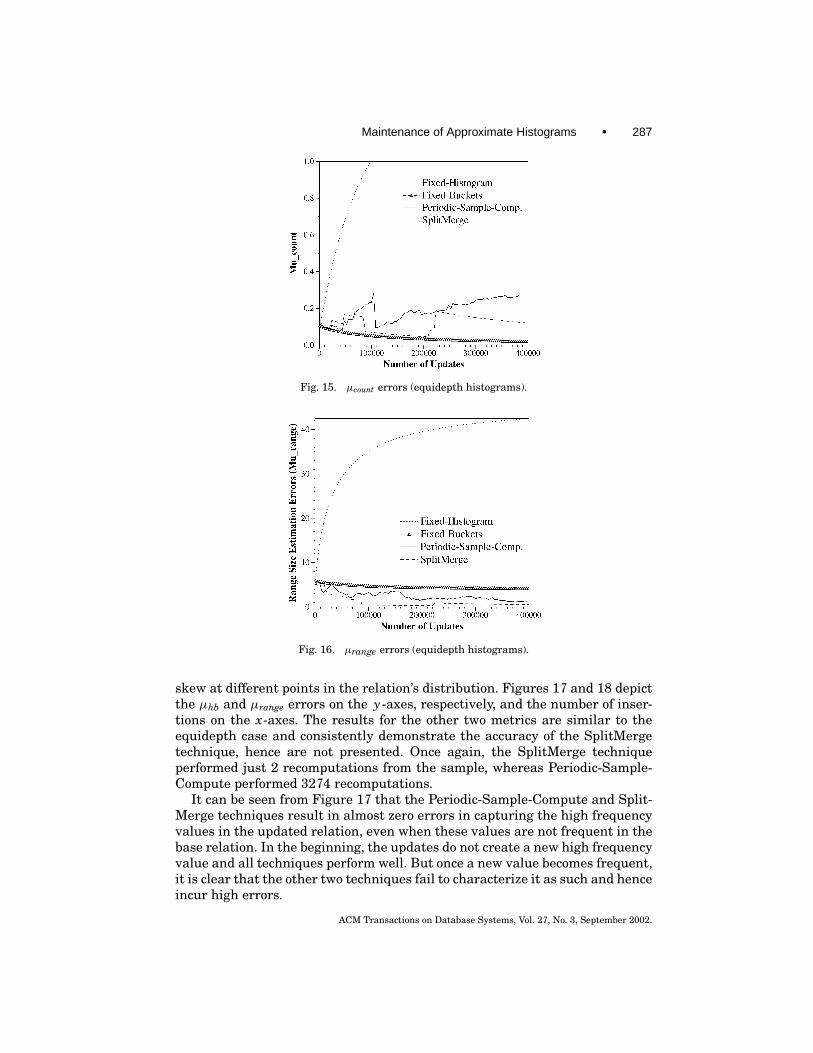
We compare the effectiveness of various techniques in approximating equidepthhistograms under insertions into the database. The results are presented foruniform base data and zipf(2,incr) update data and are fairly consistent overmost other combinations. Figures 14 through 16 depict various error measuresas a function of the number of insertions. For this experiment, the SplitMergetechnique performed just 2 recomputations from the backing sample, whereasPeriodic-Sample-Compute performed 3276.

It is clear from Figure 14 that the SplitMerge technique is nearly identicalto the more expensive Periodic-Sample-Compute technique in maintaining thehistogram close to equidepth. The Periodic-Sample-Compute technique doesnot maintain a perfectly equidepth histogram because it is recomputed fromthe backing sample which may not reflect all the insertions. The other twotechniques clearly result in a very poor equidepth histogram because they donot perform any splits of the overpopulated buckets. Figure 15 shows that theSplitMerge and Fixed-Buckets techniques are very accurate in reflecting theaccurate counts, because their bucket sizes are correctly updated after everyinsertion. For the other two techniques, the size of a bucket is always equalto N/β, hence the µcount and µed measures are identical. Finally, it is clearfrom Figure 16 that the SplitMerge technique offers the best performance inestimating range query result sizes as well.

6.4 Approximation of Compressed Histograms

We compare the effectiveness of various techniques in maintaining approximat-ing Compressed histograms. The base data distribution is zipf(1,incr) (a skeweddistribution is chosen so that the Compressed histogram will contain a few high-biased buckets) and the update distribution is zipf(2,random), which introduces



Fig. 15. µcount errors (equidepth histograms).

Fig. 16. µrange errors (equidepth histograms).

skew at different points in the relation’s distribution. Figures 17 and 18 depictthe µhb and µrange errors on the y-axes, respectively, and the number of inser-tions on the x-axes. The results for the other two metrics are similar to theequidepth case and consistently demonstrate the accuracy of the SplitMergetechnique, hence are not presented. Once again, the SplitMerge techniqueperformed just 2 recomputations from the sample, whereas Periodic-Sample-Compute performed 3274 recomputations.

It can be seen from Figure 17 that the Periodic-Sample-Compute and Split-Merge techniques result in almost zero errors in capturing the high frequencyvalues in the updated relation, even when these values are not frequent in thebase relation. In the beginning, the updates do not create a new high frequencyvalue and all techniques perform well. But once a new value becomes frequent,it is clear that the other two techniques fail to characterize it as such and henceincur high errors.



Fig. 17. µhb errors (Compressed histograms).

Fig. 18. µrange errors (Compressed histograms).

Figure 18 shows that the errors in range size estimation follow a similarpattern to that of the equidepth case. Also, as expected from our earlier work[Poosala et al. 1996], the Compressed histograms are observed to incur smallererrors than the equidepth histograms from Figure 16.

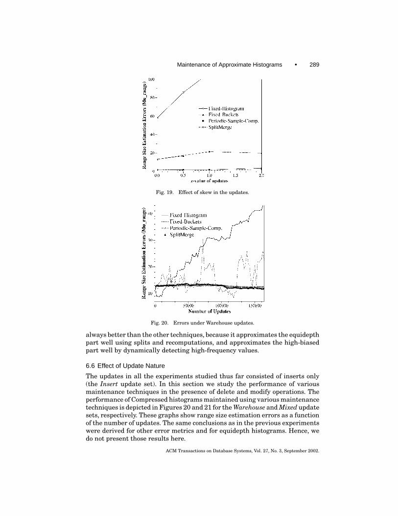
6.5 Effect of Skew in the Updates

High skew in the update data can alter the overall data distribution dra-matically, and hence requires effective histogram maintenance techniques. InFigure 19 we depict the performance of various Compressed histograms result-ing from the techniques at the end of 400 K insertions to the database. Thex-axis represents the z parameter values and the y-axis represents the errorsin estimating range query result sizes (µrange). The Fixed-Histogram techniquefails very quickly because it assumes that the updates are uniform and hencedoes not update the high-biased part correctly. It is clear from this figure thatthe SplitMerge technique performs consistently well for all levels of skew and is



Fig. 19. Effect of skew in the updates.

Fig. 20. Errors under Warehouse updates.

always better than the other techniques, because it approximates the equidepthpart well using splits and recomputations, and approximates the high-biasedpart well by dynamically detecting high-frequency values.

6.6 Effect of Update Nature

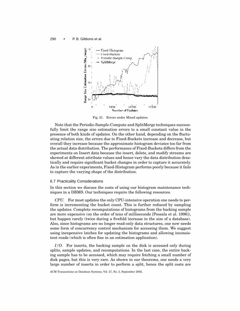
The updates in all the experiments studied thus far consisted of inserts only(the Insert update set). In this section we study the performance of variousmaintenance techniques in the presence of delete and modify operations. Theperformance of Compressed histograms maintained using various maintenancetechniques is depicted in Figures 20 and 21 for the Warehouse and Mixed updatesets, respectively. These graphs show range size estimation errors as a functionof the number of updates. The same conclusions as in the previous experimentswere derived for other error metrics and for equidepth histograms. Hence, wedo not present those results here.



Fig. 21. Errors under Mixed updates.

Note that the Periodic-Sample-Compute and SplitMerge techniques success-fully limit the range size estimation errors to a small constant value in thepresence of both kinds of updates. On the other hand, depending on the fluctu-ating relation size, the errors due to Fixed-Buckets increase and decrease, butoverall they increase because the approximate histogram deviates too far fromthe actual data distribution. The performance of Fixed-Buckets differs from theexperiments on Insert data because the insert, delete, and modify streams areskewed at different attribute values and hence vary the data distribution dras-tically and require significant bucket changes in order to capture it accurately.As in the earlier experiments, Fixed-Histogram performs poorly because it failsto capture the varying shape of the distribution.

6.7 Practicality Considerations

In this section we discuss the costs of using our histogram maintenance tech-niques in a DBMS. Our techniques require the following resources.

CPU. For most updates the only CPU-intensive operation one needs to per-form is incrementing the bucket count. This is further reduced by samplingthe updates. Complete recomputations of histograms from the backing sampleare more expensive (on the order of tens of milliseconds [Poosala et al. 1996]),but happen rarely (twice during a fivefold increase in the size of a database).Also, since histograms are no longer read-only data structures, one now needssome form of concurrency control mechanism for accessing them. We suggestusing inexpensive latches for updating the histograms and allowing inconsis-tent reads (which is often fine in an estimation application).

I/O. For inserts, the backing sample on the disk is accessed only duringsplits, sample updates, and recomputations. In the last case, the entire back-ing sample has to be accessed, which may require fetching a small number ofdisk pages, but this is very rare. As shown in our theorems, one needs a verylarge number of inserts in order to perform a split, hence the split costs are



also quite negligible. Similarly, for a large relation, the backing sample is alsoupdated very rarely. On the other hand, our techniques for arbitrary deleteand modify operations require accessing the backing sample on every sampledupdate, which may make the techniques expensive in some environments. Fordelete operations in a data warehouse environment, which houses transactionalinformation for sliding time windows, the techniques are I/O effective.

Space. Our techniques do not require any additional data in memory otherthan those already present in a histogram. On the other hand, they need diskspace (on the order of 1 to 10 pages) for the backing sample. In comparisonwith typical relation and disk sizes, this is clearly negligible (see Figure 1 foran illustration).

Overall, the above argues qualitatively that the resource requirements ofthe maintenance algorithms are negligibly small in most situations. Furtherquantitative studies in real database systems are needed in order to measurethe overheads occurring in practice.

7. CONCLUSIONS

This article proposed a novel approach for maintaining histograms and sam-ples up to date in the presence of updates to the database. This is critical forvarious DBMS components (primarily query optimizers) that rely on estimatesrequiring information about the current data. Algorithms were proposed for thewidely used equidepth histograms and the highly accurate class of Compressedhistograms. We introduced these innovations:

—The notion of a backing sample, with its advantages over previous approachesto obtaining samples, and techniques for its maintenance;

—The idea of maintaining histograms incrementally by making use of the back-ing sample. The backing sample can be much larger than the histogram andreside on the disk; it is accessed very rarely in support of the histogram,which is typically in main memory; and

—Split and merge techniques on histogram buckets, which drastically reduceaccesses to the disk for the backing sample.

Next, we conducted a large set of experiments to demonstrate the effec-tiveness of our algorithms in maintaining histograms. Our conclusions are asfollows.

—The new techniques are very effective in approximating equidepth andCompressed histograms. They are equally effective for relations orders ofmagnitude larger. In fact, as the relation size grows, the relative over-head of maintaining a backing sample with equal accuracy becomes evensmaller.

—Very few recomputations from the backing sample are incurred for a largenumber of updates, proving that our split and merge techniques are quiteeffective in minimizing the overheads due to recomputation.



—The experiments clearly show that histograms maintained using these tech-niques remain highly effective in result size estimation, unlike the previousapproaches.

The CPU, I/O, and storage requirements for these techniques are negligible forinsert-mostly databases and for data warehousing environments.

Based on our results, we recommend that these techniques be used in mostDBMSs, for effective incremental maintenance of approximate histograms.

APPENDIX

A. PROOFS FROM SECTION 3

In this section, we prove the correctness of MaintainBackingSample, as wellas various properties about the algorithm. An important assumption we use isthat the sequence of database operations is independent of the random choicesmade by our algorithm.

Let S be a set of size N . A sample of size n≤N (without replacement) fromS is a subset of size n of the elements in S. There are ( N

n ) possible samples of Sof size n. A random sample of size n is a sample of S selected with probability1/( N

n ).Our algorithm treats database insertions as in Vitter’s [1985] algorithm, so

we use the following fact shown in Vitter [1985], restated using the terminologyof this article.

OBSERVATION A.1. Let S be a set of size N, and let x be an element not inS. Let S1 be a random sample of size n of S, and let u be an element selecteduniformly at random from S1. Let S2 be constructed as follows.

S2 ={

S1 + {x} − {u} with probability n(N+1)

S1 otherwise.

Then S2 is a random sample of size n of S+{x}.

Next consider deletions. For an element just deleted from the relation R, ifthe element is in the backing sample S, our algorithm deletes it from S, else itleaves S unchanged. Lemma A.2 establishes that this maintains the propertythat S is a random sample.

LEMMA A.2. Let S be a set of size t, and let y be an element in S. Let S1 bea random sample of size s of S. Then if y is not in S1 then S2= S1−{ y}= S1 isa random sample of size s of S−{ y}. Else if y is in S1 then S2= S1−{ y} is arandom sample of size s− 1 of S−{ y}.

PROOF. In the former case ( y is not in S1), there are ( t−1s ) possible

samples of size s of S that do not contain y , each of which is equallylikely to be selected for S1. Since S2= S1, there is a one-to-one correspon-dence between samples S1 not containing y and samples S2. Thus, for any S2,Pr[S2 selected]=Pr[S1 selected |select a sample without y]= Pr[S1 selected]/



Pr[ select a sample without y], which equals

1(ts

)(

t − 1s

)(

ts

)= 1(

t − 1s

) .

In the latter case ( y is in S1), there are ( ts ) − ( t−1

s )= ( t−1s−1 ) possible samples

size s of S that contain y , each of which is equally likely to be selected for S1.There is a one-to-one correspondence between samples S1 containing y andsamples S2. Thus, for any S2, the probability S2 is selected is 1/( t−1

s−1 ).

We now proceed to prove Theorem 3.1.

PROOF OF THEOREM 3.1. Consider a sequence of insert, modify, and delete op-erations for an initially empty relation R. Let S be the sample resulting fromapplying MaintainBackingSample to the sequence, with a given L and U ,1≤ L≤U . We first prove the claim that the ids in S are a random sampleof the ids in R.

The proof is by induction on the length k of the sequence. For a sequenceof length k, let Rk be the set of ids in R resulting from applying the up-dates in the sequence to an initially empty relation R, and let Sk be theset of ids in S resulting from applying the algorithm in response to thesequence.

For the base case k= 1, the first update must be an insert for some id . Thisid is added to S, so S1={id } is a random sample of R1={id }.

Assume the claim is true for k≥1, and consider an arbitrary sequence Ak+1,of length k+ 1. The sequence Ak+1 consists of a sequence Ak of length k followedby a single update operation (an insert, a modify, or a delete). Let Rk and Sk bedefined according to Ak .

First, consider the case where the (k+ 1)st update is an insert of a newelement id . Thus Rk+1= Rk +{id }. If |Sk| +1= |Rk+1| ≤U then |Sk| = |Rk| andboth sets contain the same ids. By the algorithm, Sk+1= Sk +{id }, and theclaim holds by the inductive assumption. Else the claim holds by the inductiveassumption and Observation A.1.

Second, consider the case where the (k+ 1)st update is a modify of one ormore of the values of an element id in Rk . By the algorithm, Rk+1= Rk andSk+1= Sk , so the claim holds by the inductive assumption.

Third, consider the case where the (k+ 1)st update is a delete of an elementid in Rk . If id 6∈ Sk , then the claim holds by the inductive assumption andLemma A.2. If id ∈ Sk , then also by the inductive assumption and Lemma A.2,the ids in Sk −{id } are a random sample of the ids in Rk+1. If the algorithmscans Rk+1, then consider some sequence A′ of |Rk+1|< k inserts, one insert foreach element in Rk+1. By the inductive assumption applied to A′, the ids inSk+1 are a random sample of the ids in Rk+1.



Since in all three cases the claim holds for an arbitrary Ak+1, the claim ismaintained for all sequences of length k+ 1, and hence by induction holds forall finite length sequences.

Finally, consider the relation R after an arbitrary sequence of update oper-ations and a sample S generated by the algorithm. Since the set of ids in Sis a random sample of the set of ids in R, and the updates are independent ofthe random choices made by the algorithm, then for any attribute X of R, theset Vs=

⋃id∈S id.X of values is a random sample of the set Vr =

⋃id∈R id.X of

values. The theorem follows.

MaintainBackingSample maintains a backing sample S such thatmin(|R|, L)≤ |S| ≤U , where L and U are prespecified upper and lower bounds.It populates S up to U elements and then a series of U − L+ 1 deletes of sampleelements are needed in order to force the algorithm to rescan the relation R inorder to repopulate S. The next lemma shows that rescans are expected to beinfrequent for large relations.

LEMMA A.3. Consider an initial relation R and a backing sample S for R ofsize U. Consider any sequence of updates to R and let N0≥U be a lower boundon the size of R after each such update. (There is no upper bound imposed on|R|.) Then at most one rescan is expected every N0(U − L+ 1)/U updates.

PROOF. Initially, |S| =U , so a series of U − L+ 1 deletes of sample elementsis needed in order to force a rescan of R. At any time, the probability that anid selected for deletion is in S is |S|/|R| (since ( |R|−1

|S|−1 )/( |R||S| ) = |S|/|R|). Since|S|/|R| ≤U/N0, the expected number of deletions needed is at least N0(U −L+ 1)/U . After the rescan, |S| =U , and the argument can be repeated.

As an example, consider a relation of size N = 2N0 and L=U/2+ 1. Then inorder to force a rescan, we must delete half of the relation. Moreover, in suchcases, the number of tuples to be rescanned is N/2, which can be amortizedagainst the N/2 deletions needed to force the rescan.

B. PROOFS FROM SECTION 4

To simplify the presentation of the proofs that follow, we ignore the use of floorsand ceilings in the algorithms.

PROOF OF THEOREM 4.1. Since each bucket count is set to N/β, µed=µcount forthis algorithm. We assume without loss of generality that all values are distinct;this can be accomplished by appending to each original value a unique label.

The probability that sampling with replacement will pick m distinct elementsis

N (N − 1)(N − 2) · · · (N −m+ 1)Nm ≥

(N −m

N

)m

=(

1− mN

)m≥ 1− m2

N.

Since m≤N 1/3, the probability is at least 1− 1/N1/3. Thus we ignore the differ-ence between sampling with and without replacement by considering whicheverone is more suited to the analysis, and compensate by subtracting N−1/3 from



the probability of obtaining the stated bounds. (This can be argued formallyusing conditioned events.)

By Lemma 7.1 in Reif and Valiant [1987], for each bucket Bi,

Pr

{f Bi ∈

[(1±

(mβ

)−1/6)

Nβ

]}≥ 1− 2√

c lnββ−√

c ,

which is greater than 1−β−√

c. Thus f Bi is within the above range for all i withprobability at least 1− β−(

√c−1). This implies that, with the same probability,

µed ≤ β

N

√√√√1β

β∑i=1

(Nβ

(mβ

)−1/6)2

=(

mβ

)−1/6

.

The theorem follows.

PROOF OF THEOREM 4.2. Consider some phase in the EquiDepthSimple algo-rithm, at which the relation is of size N . At the beginning of the phase, letN ′ be the size of the relation, and let µ′count and µ′ed be the errors µcount andµed, respectively. Let ρ ′ = 1−β − (

√c−1)− (N ′)−1/3, and let ρ= 1−β−(

√c−1)− (N/

(2+ γ ))−1/3. Since during a phase N ≤N ′(2+ γ ), we have ρ ≤ ρ ′. By Theorem 4.1,µ′ed=µ′count≤α with probability at least ρ ′, and hence at least ρ.

During a phase, a value inserted into bucket Bi increments both f Bi andBi.count. Therefore, by the definition of µcount (Equation 1), its value doesnot change during a phase, and hence at any time during the phase µcount=µ′count≤α with probability ρ. It remains to bound µed.

Let f ′Biand Bi.count′ be the values of f Bi and Bi.count, respectively, at the

beginning of the phase. Let 1′i = f ′Bi−N ′/β, and let 1i = f Bi −N/β. We claim

that |1i −1′i| ≤ (1+ γ )N ′/β. Note that |1i −1′i| ≤ max( f Bi − f ′Bi, N/β −N ′/β).

The claim follows since f Bi − f ′Bi= Bi.count− Bi.count′ ≤T − Bi.count′ =

(2+ γ )N ′/β −N ′/β, and N −N ′ ≤β(Bi.count− Bi.count′).By the claim,

1i2 ≤ (1′i + (1+ γ ) N ′/β)2 = 1′i2 + 21′i(1+ γ ) N ′/β + ((1+ γ ) N ′/β)2.

Note that∑β

i=11′i =

∑β

i=1( f Bi − N ′/β) = 0. Hence, substituting for 12i in the

definition of µed (Equation (2)) we obtain

µed = β

N

√√√√1β

(β∑i

1′i2 +

β∑i=1

((1+ γ )N ′/β)2

)

≤ µ′ed+β

N(1+ γ ) N ′/β ≤µ′ed+ (1+ γ ).

The theorem follows.

PROOF OF LEMMA 4.5. Let N ′ be the total number of elements at the beginningof a phase t. Note that the sum of the bucket counts at the start of phase t is N ′.Each new element increases this sum by one, and both splitting and merginghave no effect on this sum. Thus throughout phase t, the sum of the bucketcounts is always exactly the number of elements.



Consider first the case that γ >0. Recall that a phase ends when there isno pair of adjacent buckets Bi and Bi+1 such that Bi.count+ Bi+1.count<T .Therefore, summing over the pairs, {B2 j−1, B2 j } for j = 1, 2, . . . , β/2 we ob-tain that the sum of the bucket counts (and hence the total number of el-ements) at the end of phase t is at least (β/2) · T =β/2 · (2 + γ ) · N ′/β =(1+ γ /2)N ′.

For the case−1<γ ≤ 0 we note that a bucket can get to be of size T only aftergetting (1+ γ )N ′/β new elements. Therefore the total number of elements atthe end of the phase is at least (1+ (1+ γ )/β)N ′.

Thus in either case, the number of phases after N inserts is at most logα N .The lemma follows because the number of phases is also upper bounded by thenumber of inserts.

ACKNOWLEDGMENTS

We acknowledge the contributions of Andy Witkowski to the algorithm formaintaining approximate equidepth histograms. We also thank Nabil Kahaleand Sridhar Rajagopalan for discussions related to this work. Finally, wethank the anonymous referees for their helpful comments on improving thearticle.

REFERENCES

ABOULNAGA, A. AND CHAUDHURI, S. 1999. Self-tuning histograms: Building histograms withoutlooking at data. In Proceedings of the ACM SIGMOD International Conference on Managementof Data, ACM, Philadelphia, 181–192.

ACHARYA, S., GIBBONS, P. B., AND POOSALA, V. 2000. Congressional samples for approximate an-swering of group-by queries. In Proceedings of the ACM SIGMOD International Conference onManagement of Data, ACM, Dallas, 487–498.

ACHARYA, S., GIBBONS, P. B., POOSALA, V., AND RAMASWAMY, S. 1999. Join synopses for approximatequery answering. In Proceedings of the ACM SIGMOD International Conference on Managementof Data, ACM, Philadelphia, 275–286.

BLOHSFELD, B., KORUS, D., AND SEEGER, B. 1999. A comparison of selectivity estimators for rangequeries on metric attributes. In Proceedings of the ACM SIGMOD International Conference onManagement of Data, ACM, Philadelphia, 238–250.

BRUNO, N., CHAUDHURI, S., AND GRAVANO, L. 2001. STHoles: A multidimensional workload-awarehistogram. In Proceedings of the ACM SIGMOD International Conference on Management ofData, ACM, Santa Barbara, CA, 211–222.

CHAUDHURI, S., DAS, G., AND NARASAYYA, V. 2001. A robust, optimization-based approach for ap-proximate answering of aggregate queries. In Proceedings of the ACM SIGMOD InternationalConference on Management of Data, ACM, Santa Barbara, CA, 295–306.

CHAUDHURI, S., MOTWANI, R., AND NARASAYYA, V. 1998. Random sampling for histogram construc-tion: How much is enough? In Proceedings of the ACM SIGMOD International Conference onManagement of Data, ACM, Seattle, 436–447.

CHRISTODOULAKIS, S. 1984. Implications of certain assumptions in database performance evalua-tion. ACM Trans. Database Syst. 9, 2 (June), 163–186.

DESHPANDE, A., GAROFALAKIS, M., AND RASTOGI, R. 2001. Independence is good: Dependency-basedhistogram synopses for high-dimensional data. In Proceedings of the ACM SIGMOD InternationalConference on Management of Data, ACM, Santa Barbara, CA, 199–210.

GANTI, V., LEE, M.-L., AND RAMAKRISHNAN, R. 2000. ICICLES: Self-tuning samples for approximatequery answering. In Proceedings of the 26th International Conference on Very Large Data Bases,Morgan Kaufman, Cairo, 176–187.



GIBBONS, P. B. 2001. Distinct sampling for highly-accurate answers to distinct values queries andevent reports. In Proceedings of the 27th International Conference on Very Large Data Bases,Morgan Kaufman, Rome, 541–550.

GIBBONS, P. B. AND MATIAS, Y. 1998. New sampling-based summary statistics for improving ap-proximate query answers. In Proceedings of the ACM SIGMOD International Conference onManagement of Data, ACM, Seattle, 331–342.

GILBERT, A., GUHA, S., INDYK, P., KOTIDIS, Y., MUTHUKRISHNAN, S., AND STRAUSS, M. J. 2002a. Fastsmall-space algorithms for approximate histogram maintenance. In Proceedings of the 34th ACMSymposium on the Theory of Computing, ACM, Montreal.

GILBERT, A. C., KOTIDIS, Y., MUTHUKRISHNAN, S., AND STRAUSS, M. J. 2002b. How to summarize theuniverse: Dynamic maintenance of quantiles. In Proceedings of the 28th International Conferenceon Very Large Data Bases, Morgan Kaufman, Hong Kong.

GREENWALD, M. AND KHANNA, S. 2001. Space-efficient online computation of quantile summaries.In Proceedings of the ACM SIGMOD International Conference on Management of Data, ACM,Santa Barbara, CA, 58–66.

GUHA, S., KOUDAS, N., AND SHIM, K. 2001. Data-streams and histograms. In Proceedings of the 33rdACM Symposium on Theory of Computing, ACM, Hersonissos, Crete, 471–475.

GUNOPULOS, D., KOLLIOS, G., TSOTRAS, V. J., AND DOMENICONI, C. 2000. Approximating multi-dimensional aggregate range queries over real attributes. In Proceedings of the ACM SIGMODInternational Conference on Management of Data, ACM, Dallas, 463–474.

IOANNIDIS, Y. AND CHRISTODOULAKIS, S. 1991. On the propagation of errors in the size of join results.In Proceedings of the ACM SIGMOD Conference on Management of Data, ACM, Denver, 268–277.

IOANNIDIS, Y. AND POOSALA, V. 1999. Histogram-based techniques for approximating set-valuedquery-answers. In Proceedings of the 25th International Conference on Very Large Databases,Morgan Kaufman, Edinburgh, 174–185.

JAGADISH, H. V., KOUDAS, N., MUTHUKRISHNAN, S., POOSALA, V., SEVCIK, K., AND SUEL, T. 1998. Optimalhistograms with quality guarantees. In Proceedings of the 24th International Conferece on VeryLarge Data Bases, Morgan Kaufman, New York, 275–286.

KONIG, A. C. AND WEIKUM, G. 1999. Combining histograms and parametric curve fitting forfeedback-driven query result-size estimation. In Proceedings of the 25th International Confer-ence on Very Large Databases, Morgan Kaufman, Edinburgh, 423–434.

KOOI, R. P. 1980. The optimization of queries in relational databases. PhD Thesis, Case WesternReserve University.

LIPTON, R. J., NAUGHTON, J. F., AND SCHNEIDER, D. A. 1990. Practical selectivity estimation throughadaptive sampling. In Proceedings of the ACM SIGMOD Conference on Management of Data,ACM, Atlantic City, NJ, 1–11.

MATIAS, Y., VITTER, J. S., AND WANG, M. 1998. Wavelet-based histograms for selectivity estimation.In Proceedings of the ACM SIGMOD International Conference on Management of Data, ACM,Seattle, 448–459.

MATIAS, Y., VITTER, J. S., AND WANG, M. 2000. Dynamic maintenance of wavelet-based histograms.In Proceedings of the 26th International Conference on Very Large Data Bases, Morgan Kaufman,Cairo, 101–110.

POOSALA, V. 1997. Histogram-based estimation techniques in database systems. PhD Thesis, Uni-versity of Wisconsin-Madison.

POOSALA, V. AND IOANNIDIS, Y. 1996. Estimation of query-result distribution and its application inparallel-join load balancing. In Proceedings of the 22nd International Conference on Very LargeDatabases, VLDB, Bombay, 448–459.

POOSALA, V. AND IOANNIDIS, Y. 1997. Selectivity estimation without the attribute value indepen-dence assumption. In Proceedings of the 23rd International Conference on Very Large Data Bases,Morgan Kaufman, Athens, 486–495.

POOSALA, V., IOANNIDIS, Y., HAAS, P., AND SHEKITA, E. 1996. Improved histograms for selectivityestimation of range predicates. In Proceedings of the ACM SIGMOD Conference on Managementof Data, ACM, Montreal, 294–305.

REIF, J. H. AND VALIANT, L. G. 1987. A logarithmic time sort for linear size networks. J. ACM 34, 1,60–76.



SELINGER, P. G., ASTRAHAN, M. M., CHAMBERLIN, D. D., LORIE, R. A., AND PRICE, T. T. 1979. Accesspath selection in a relational database management system. In Proceedings of the ACM SIGMODConference on Management of Data, ACM, Boston, 23–34.

VITTER, J. S. 1985. Random sampling with a reservoir. ACM Trans. Math. Softw. 11, 37–57.ZIPF, G. K. 1949. Human Behaviour and the Principle of Least Effort. Addison-Wesley, Reading,

Mass.

Received February 2001; revised August 2002; accepted August 2002


Fast Incremental Maintenance of Approximate...

Documents

Transcript of Fast Incremental Maintenance of Approximate...