Fast Fourier transform with examples inMATLAB

Parsiad Azimzadeh

Contents1 Introduction 1

2 Discrete Fourier transform 22.1 Roots of unity . . . . . . . . . . . . . . . . . . . . . . . . . . . . . 22.2 Forward and inverse transforms . . . . . . . . . . . . . . . . . . . 32.3 Some immediate results . . . . . . . . . . . . . . . . . . . . . . . 42.4 Convolution and cross-correlation . . . . . . . . . . . . . . . . . . 52.5 Real signals . . . . . . . . . . . . . . . . . . . . . . . . . . . . . . 6

3 Fast Fourier transform 73.1 Radix-2 algorithm . . . . . . . . . . . . . . . . . . . . . . . . . . 83.2 Periodicity error (a.k.a. wrap-around error) . . . . . . . . . . . . 8

4 Image compression (with MATLAB code) 10

1 IntroductionIn mathematics, the discrete Fourier transform (DFT) converts a finite list ofequally spaced samples of a function into the list of coefficients of a finite com-bination of complex sinusoids, ordered by their frequencies, that has those samesample values. It can be said to convert the sampled function from its originaldomain (often time or position along a line) to the frequency domain.

The DFT is the most important discrete transform, used to perform Fourieranalysis in many practical applications. In digital signal processing, the functionis any quantity or signal that varies over time, such as the pressure of a soundwave, a radio signal, or daily temperature readings, sampled over a finite timeinterval (often defined by a window function). In image processing, the samplescan be the values of pixels along a row or column of a raster image. The DFT isalso used to efficiently solve partial differential equations, and to perform otheroperations such as convolutions or multiplying large integers.

A fast Fourier transform (FFT) is an algorithm to compute the DFT and itsinverse. Fourier analysis converts time (or space) to frequency and vice versa; an

1

FFT rapidly computes such transformations by factorizing the DFT matrix intoa product of sparse (mostly zero) factors. As a result, fast Fourier transformsare widely used for many applications in engineering, science, and mathematics.The basic ideas were popularized in 1965, but some FFTs had been previouslyknown as early as 1805. Fast Fourier transforms have been described as “themost important numerical algorithm[s] of our lifetime”.

2 Discrete Fourier transform

2.1 Roots of unityDefinition 1 (Roots of unity in C). Let n be a positive integer. z ∈ C is saidto be an n-th root of unity if and only if zn = 1.

Corollary 2. If z is an n-th root of unity, so too is zw for any w ∈ C.

Proof. Follows immediately from the definition: (zw)n

= (zn)w

= 1w = 1.

Corollary 3. Let n be a positive integer and ωn ≡ e−2πi/n.{ωjn}n−1j=0

are then-th roots of unity.

Proof. It is easily verified that these are indeed n-th roots of unity:(ωjn)n

=ωjnn = e−2πij = 1. Since zn is an n-th degree polynomial, the fundamentaltheorem of algebra yields there are no other such roots.

Definition 4 (Kronecker Delta). The Kronecker delta, δi,j , is defined to be 1if and only if i = j and zero otherwise. That is,

δi,j ≡

{1 if i = j

0 otherwise.

Lemma 5. Let n be a positive integer and z 6= 1 be an n-th root of unity. Then∑n−1m=0 z

m = 0.

Proof. Being a finite geometric series, we can write

n−1∑m=0

zm =1− zn

1− z.

Since zn is an n-th root of unity, the above is zero.

Corollary 6. Let n be a positive and integer and 0 ≤ j, j′ < n. Then

n−1∑k=0

ω(j−j′)kn = nδj,j′ .

Proof. If j = j′, the sum above reduces to∑n−1k=0 1 = n. Otherwise, ωj−j

′

n 6= 1is an n-th root of unity (Corollary 2) and the result follows.

2

Remark 7. Denote by z† the conjugate transpose of z. Similarly, for a scalar z,denote by z its conjugate.

Theorem 8 (Orthogonality). Let uj ∈ Cn with

uj ≡⟨ω0n, ωjn, ω2j

n , . . . , ω(n−1)jn

⟩.

{uj}n−1j=0

is an orthogonal basis for Cn.

Proof. Using Corollary 6,

⟨uj ,uj

′⟩

=(uj

′)†

uj =

n−1∑k=0

ω−j′k

n ωjkn =

n−1∑k=0

ω(j−j′)kn = nδj,j′ .

2.2 Forward and inverse transformsIntuitively, the forward transform takes a signal from its original domain to thefrequency domain. The inverse transform does the reverse.

Remark 9 (Indexing vectors). Denote by [z]k and zk the k-th index of a vectorz. Vector indices in this exposition start at 0 to simplify modulo arithmetic.

Definition 10 (Forward and inverse transforms). Let F : Cn → Cn, the for-ward Fourier transform, be defined by

[Fx]k ≡n−1∑j=0

xjωjkn

and F−1 : Cn → Cn, the inverse Fourier transform, by

[F−1X

]j≡ 1

n

n−1∑k=0

Xkω−jkn .

Theorem 11 (Invertibility). F−1 is the inverse of F .

Proof. Let x ∈ Cn and X ≡ Fx. Then

[F−1X

]j

=1

n

n−1∑k=0

n−1∑j′=0

xj′ωj′kn

ω−jkn

=1

n

n−1∑j′=0

xj′n−1∑k=0

ω(j−j′)kn =

1

n

n−1∑j′=0

xj′nδj,j′ = xj .

3

Remark 12 (Vector-scalar multiply). Many software libraries do not provide aninterface to F−1 directly and instead define an “inverse” transform G by

[GX]j ≡n−1∑k=0

Xkω−jkn .

Note that F−1X = GX/n. This avoids the need for the extra vector-scalarmultiply with 1/n for performance. For example, MATLAB uses the definitionsof F and F−1 given here for their fft and ifft functions. The popular softwarelibrary FFTW, does not.

2.3 Some immediate resultsTheorem 13 (Plancherel theorem). Let x,y ∈ Cn, X ≡ Fx, and Y ≡ Fy.Then

〈x,y〉 =1

n〈X,Y〉 .

Proof. First, note that

XkYk =

n−1∑j=0

xjωjkn

n−1∑j′=0

yj′ω−j′kn

=

n−1∑j,j′=0

xjyj′ω(j−j′)kn

and hencen−1∑k=0

XkYk =

n−1∑j,j′=0

xjyj′n−1∑k=0

ω(j−j′)kn =

n−1∑j,j′=0

xjyj′nδj,j′ = n

n−1∑j=0

xjyj

as desired.

Corollary 14 (Parseval’s theorem). Let x ∈ Cn and X ≡ Fx. Then

〈x,x〉 =1

n〈X,X〉 .

Proof. Follows from the Plancherel theorem by taking x = y.

Lemma 15 (Periodicity). Let x ∈ Cn and X ≡ Fx. Then Xk+mn = Xk forany integer m (the same result can be established for the inverse transform).

Proof. This follows immediately from the definition of F :

Xk+mn =

n−1∑j=0

xjωj(k+mn)n =

n−1∑j=0

xjωjkn ω

jmnn =

n−1∑j=0

xjωjkn = Xk.

Theorem 16 (Shift theorem). Let x ∈ Cn and x′ be defined by x′j ≡ ωjmn xj.Let X ≡ Fx and X′ ≡ Fx′. Then X′k = Xk−m.

4

2.4 Convolution and cross-correlationThe DFT provides an alternative way to compute the convolution and cross-correlation of signals of length n. These calculations, naïvely, require Θ

(n2)

floating point operations (FLOPs). FFTs reduce this to Θ (n log n).

Remark 17. Denote by a mod b the least nonegative residue of j modulo n(this is not its most common usage, in which it denotes instead an equivalenceclass). For example, 3 mod 2 = 1 (as opposed to the usual 3 mod 2 = [1] ={. . . ,−4,−2, 1, 3, 5, . . .}).Remark 18 (Periodicity). For the remainder of this document, vectors are ex-tended as follows: if x ∈ Cn, define

xj ≡ [x]j ≡ xj mod n if j < 0 or j ≥ n.

Definition 19 (Circular convolution). The circular convolution of vectors x,y ∈Cn is a vector x ∗ y ∈ Cn defined by

[x ∗ y]j ≡n−1∑`=0

x`yj−`.

Remark 20. Denote by x ◦ y the element-wise product of (finite) vectors x andy.

Theorem 21 (Convolution theorem). Let x,y ∈ Cn, X ≡ Fx, and Y ≡ Fy.Then,

F−1 {X ◦Y} = x ∗ y.

Proof. First, note that

XkYk =

(n−1∑`=0

x`ω`kn

)(n−1∑`′=0

y`′ω`′kn

)=

n−1∑`,`′=0

x`y`′ω(`+`′)kn .

From this, it follows that

[F−1 {X ◦Y}

]j

=1

n

n−1∑k=0

n−1∑`,`′=0

x`y`′ω(`+`′)kn ω−jkn

=1

n

n−1∑`,`′=0

x`y`′n−1∑k=0

ω(`+`′−j)kn .

Since 0 ≤ `, `′ < n, we cannot use Corollary 6 directly. Note, however, that asimilar argument yields

n−1∑k=0

ω(`+`′−j)kn = nδ(`+`′) mod nj .

5

Since δ(`+`′) mod n,j = 1 exactly when (`+ `′) mod n = j (equivalently (j − `′) mod n =`), [

F−1 {X ◦Y}]j

=

n−1∑j=0

x`y`−j

as desired.

Remark 22. The proofs of Theorems 23, 25, and 26 are identical in strategy andthus omitted.

Theorem 23 (Convolution theorem (dual)). Let X,Y ∈ Cn, x ≡ F−1X, andy ≡ F−1Y. Then,

F {x ◦ y} = X ∗Y.

Definition 24 (Circular cross-correlation). The circular cross-correlation ofvectors x,y ∈ Cn is a vector x ? y ∈ Cn defined by

[x ? y]j ≡n∑`=0

x`yj+`.

Theorem 25 (Cross-correlation theorem). Let x,y ∈ Cn, X ≡ Fx, and Y ≡Fy. Then,

F−1{X† ◦Y

}= x ? y.

Theorem 26 (Cross-correlation theorem (dual)). Let X,Y ∈ Cn, x ≡ F−1Xand y ≡ F−1Y. Then,

F{x† ◦ y

}= X ?Y.

2.5 Real signalsIn practice, the input to the forward transform is often a real signal (i.e. avector in Rn). It is useful to derive some facts about such signals.

Theorem 27 (Conjugate symmetry). Let x ∈ Rn and X ≡ Fx. For 0 < k < n,Xk = Xn−k.

Proof. Since the conjugate of a real scalar is itself,

Xk =

n−1∑j=0

xjωjkn =

n−1∑j=0

xjω−jkn = Xn−k.

Theorem 28. Let x,y ∈ Rn and z ≡ x + iy. Further let X ≡ Fx, Y ≡ Fy,and Z ≡ Fz. Then,

Xk =Zk + Zn−k

2and

Yk =Zk − Zn−k

2.

6

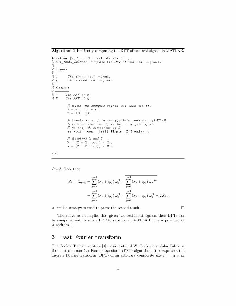
Algorithm 1 Efficiently computing the DFT of two real signals in MATLAB.

function [X, Y] = f f t_ r e a l_ s i gna l s (x , y )% FFT_REAL_SIGNALS Computes the DFT of two r ea l s i g n a l s .%% Inputs% −−−−−−% x The f i r s t r e a l s i g n a l .% y The second r ea l s i g n a l .%% Outputs% −−−−−−−% X The FFT of x% Y The FFT of y

% Bui ld the complex s i g n a l and take i t s FFTz = x + 1 . i ∗ y ;Z = f f t ( z ) ;

% Create Zr_conj , whose ( j+1)− th component (MATLAB% ind i c e s s t a r t at 1) i s the conjugate o f the% (n−j+1)− th component o f ZZr_conj = conj ( [ Z(1 ) f l i p l r (Z ( 2 :end ) ) ] ) ;

% Retr ieve X and YX = (Z + Zr_conj ) / 2 . ;Y = (Z − Zr_conj ) / 2 . ;

end

Proof. Note that

Zk + Zn−k =

n−1∑j=0

(xj + iyj)ωjkn +

n−1∑j=0

(xj + iyj)ω−jkn

=

n−1∑j=0

(xj + iyj)ωjkn +

n−1∑j=0

(xj − iyj)ωjkn = 2Xk.

A similar strategy is used to prove the second result.

The above result implies that given two real input signals, their DFTs canbe computed with a single FFT to save work. MATLAB code is provided inAlgorithm 1.

3 Fast Fourier transformThe Cooley–Tukey algorithm [1], named after J.W. Cooley and John Tukey, isthe most common fast Fourier transform (FFT) algorithm. It re-expresses thediscrete Fourier transform (DFT) of an arbitrary composite size n = n1n2 in

7

terms of smaller DFTs of sizes n1 and n2 recursively, in order to reduce thecomputation time to Θ (n log n).

3.1 Radix-2 algorithmThe radix-2 algorithm coresponds to the case of n1 = n2 = n/2 (hence the name"radix-2"). That is, it divides a DFT of size n into two interleaved DFTs of sizen/2 with each recursive stage. The motivation comes from considering X ≡ Fxfor x ∈ Cn:

Xk =

n−1∑j=0

xjωjkn

=

n/2−1∑j=0

x2jω2jkn +

n/2−1∑j=0

x2j+1ω(2j+1)kn

=

n/2−1∑j=0

x2jω2jkn + ωkn

n/2−1∑j=0

x2j+1ω2jkn

= Ek + ωknOk

where E and O are the DFTs of the even and odd parts of the original signalx, respectively. Since

ωk+n/2n = e−πiωkn = −ωkn,

by the periodicity of the DFT, the above is further simplified to the two equa-tions

Xk = Ek + ωknOk

Xk+n/2 = Ek − ωknOk

for 0 ≤ k < n/2. The flow of data in this algorithm is represented pictorially inFigure 1.

3.2 Periodicity error (a.k.a. wrap-around error)It is often the case that we do not wish to compute the circular convolutionand circular cross-correlations of vectors, but rather (noncircular) convolutionsand (noncircular) cross-correlations. However, doing so by the FFT approachdescribed above introduces error. This issue is resolved by introducing stringsof zeros into the original input signals prior to the procedure.

Definition 29 (Convolution). The (noncircular) convolution of vectors x,y ∈Cn is a vector x∗y ∈ Cn defined by

8

Figure 1: The “butterfly” diagram depicting the flow of data in the radix-2algorithm (CC BY 3.0, by Wikimedia user Virens).

[x∗y]j ≡j∑`=0

x`yj−`.

respectively.

Corollary 30. The error incurred from approximating a noncircular convolu-tion with a circular convolution is

∣∣∣[x ∗ y]j − [x∗y]j

∣∣∣ ≡∣∣∣∣∣∣n−1∑`=j+1

x`yj−`

∣∣∣∣∣∣ .Theorem 31 (Fixing periodicity error in a convolution). Let x,y ∈ Cn andx, y ∈ C2n−1 such that xj = xj and yj = yj for 0 ≤ j < n and xj = yj = 0 forn ≤ j < 2n− 1. Then for 0 ≤ j < n,

[x ∗ y]j = [x∗y]j .

Proof. Note that

[x ∗ y]j ≡2n−2∑`=0

x`yj−` =

n−1∑`=0

x`yj−` +

2n−2∑`=n

x`︸︷︷︸0

yj−` =

n−1∑`=0

x`yj−`

and since yj−` = 0 whenever j < ` < n and yj−` = yj−` whenever 0 ≤ ` ≤ j,the desired result follows.

9

Definition 32 (Cross-correlation). The (noncircular) cross-correlation of vec-tors x,y ∈ Cn is a vector x ?′ y ∈ Cn defined by

[x?y]j ≡n−1−j∑`=0

x`yj+`.

Theorem 33 (Fixing periodicity error in a cross-correlation). Let x,y ∈ Cnand x, y ∈ C2n−1 such that xj = xj and yj = yj for 0 ≤ j < n and xj = yj = 0for n ≤ j < 2n− 1. Then for 0 ≤ j < n,

[x ? y]j = [x?y]j .

4 Image compression (with MATLAB code)Image compression is one possible use of the DFT. It can be achieved by(1) transforming to the frequency-domain via a DFT and (2) dropping high-frequency components. The more high-frequency components are dropped, themore space is saved (while simultaneously lowering the quality of the image).To retrieve the original image, one must transform back to the original domain.Algorithm 2 gives a MATLAB implementation. Figure 2 shows the results ofthis algorithm.

References[1] James W Cooley and John W Tukey. An algorithm for the machine calcula-

tion of complex fourier series. Mathematics of computation, 19(90):297–301,1965.

10

Algorithm 2 MATLAB code for image compression.

function [ dft_R , dft_G , dft_B ] = compress_image ( image , r a t i o )% COMPRESS_IMAGE Compresses an image .%% Inputs% −−−−−−% image The o r i g i n a l image .% ra t i o The compression r a t i o in ( 0 , 1 ] . 1 f o r no compression .%% Outputs% −−−−−−−% dft_R The d i s c r e t e Fourier transform of the red channel% a f t e r removing high f r e quenc i e s .% dft_G The d i s c r e t e Fourier transform of the green channel% a f t e r removing high f r e quenc i e s .% dft_B The d i s c r e t e Fourier transform of the b lue channel% a f t e r removing high f r e quenc i e s .

% Normalizeimage_d = double ( image) / double (max (max (max ( image ) ) ) ) ;

% FFTcompressed_image = f f t2 ( image_d ) ;dft_R = sparse ( compressed_image ( : , : , 1 ) ) ;dft_G = sparse ( compressed_image ( : , : , 2 ) ) ;dft_B = sparse ( compressed_image ( : , : , 3 ) ) ;

% Size o f image[m, n , ~] = s ize ( image ) ;p = ce i l (m / 2 ) ;q = ce i l (n / 2 ) ;

% Number o f p i x e l s to remove from width and he i gh tf = (1 − sqrt ( r a t i o ) ) / 2 ;dm = round ( f ∗ m) ;dn = round ( f ∗ n ) ;

% The new image w l i l on ly have s q r t ( r )∗m ∗ s q r t ( r )∗n = r∗m∗n% f r e quenc i e sX = p − dm + 1 : p + dm;Y = q − dn + 1 : q + dn ;dft_R(X, : ) = 0 ;dft_R ( : , Y) = 0 ;dft_G(X, : ) = 0 ;dft_G ( : , Y) = 0 ;dft_B(X, : ) = 0 ;dft_B ( : , Y) = 0 ;

end

11

Algorithm 3 MATLAB code for image decompression.

function [ image ] = decompress_image (dft_R , dft_G , dft_B)% DECOMPRESS_IMAGE Returns a f u l l r ep r e s en ta t i on o f the image .%% Inputs% −−−−−−% dft_R The compressed red channel .% dft_G The compressed green channel .% dft_B The compressed b lue channel .%% Outputs% −−−−−−−% image The uncompressed image .

[m, n ] = s ize ( dft_R ) ;image = zeros (m, n , 3 ) ;image ( : , : , 1) = real ( i f f t 2 ( f u l l ( dft_R ) ) ) ;image ( : , : , 2) = real ( i f f t 2 ( f u l l (dft_G ) ) ) ;image ( : , : , 3) = real ( i f f t 2 ( f u l l ( dft_B ) ) ) ;

end

Algorithm 4 MATLAB code used to create example.

% Load the imageearth = imread ( ’ earth . png ’ ) ;

% Compression r a t i or a t i o = 0 . 1 5 ;

% DFT the image channels and drop high f r e quenc i e s[ dft_R , dft_G , dft_B ] = compress_image ( earth , r a t i o ) ;

% dft_∗ are s to red as sparse complex matr ices so t ha t zero en t r i e s% do not con t r i bu t e to the s to red s i z e s o f dft_∗

% To view the image , we have to turn perform an inve r s e DFT:imshow ( decompress_image (dft_R , dft_G , dft_B ) ) ;

12

(a) No compression (706 kilobytes).

(b) 15% data retention (106 kilobytes).

Figure 2: An image with varying compression ratios.

13