fast decoupled power flow for unbalanced radial distribution system
77
1 FAST DECOUPLED POWER FLOW FOR UNBALANCED RADIAL DISTRIBUTION SYSTEM Thesis submitted in partial fulfillment of the requirements for the award of degree of Master of Engineering in Power Systems & Electric Drives Thapar University, Patiala By: Kuldeep Singh (Regn. No. 80741012) Under the supervision of: Ms. Suman Bhullar Lecturer, EIED ELECTRICAL & INSTRUMENTATION ENGINEERING DEPARTMENT THAPAR UNIVERSITY PATIALA – 147004 JUNE - 2009
Transcript of fast decoupled power flow for unbalanced radial distribution system
1
FAST DECOUPLED POWER FLOW FOR
UNBALANCED RADIAL DISTRIBUTION SYSTEM
Thesis submitted in partial fulfillment of the requirements for the award of
degree of
Master of Engineering
in
Power Systems & Electric Drives
Thapar University, Patiala
By:Kuldeep Singh
(Regn. No. 80741012)
Under the supervision of:Ms. Suman Bhullar
Lecturer, EIED
ELECTRICAL & INSTRUMENTATION ENGINEERING DEPARTMENTTHAPAR UNIVERSITY
PATIALA – 147004
JUNE - 2009

2
DEDICATED
TO
MY PARENTS

3

4

5
ABSTRACT
Now these days load flow is a very important and fundamental tool for the analysis of any power
system and is used in the operational as well as planning stages. Certain applications, particularly
in distribution automation and optimization of a power system, require repeated load flow
solutions. In these applications it is very important to solve the load flow problem as efficiently
as possible. Since the invention and widespread use of digital computers and many methods for
solving the load flow problem have been developed. Most of the methods have “grown up”
around transmission systems and, over the years, variations of the Newton method such as the
fast decoupled method, have become the most widely used.
The assumptions necessary for the simplifications used in the standard fast decoupled Newton
method often are not valid in distribution systems. In particular, R/X ratios can be much higher.
However, some work has been done to attempt to overcome these difficulties.
Some of the methods based on the general meshed topology of a typical transmission system are
also applicable to distribution systems which typically have a radial or tree structure.
Specifically, we will compare the proposed method to the standard Newton method, and the
implicit Zbus Gauss method. These methods do not explicitly exploit the radial structure of the
system and therefore require the solution of a set of equations whose size is of the order of the
number of buses.
Our goal was to develop a formulation and solution algorithm for solving load flow in large
three-phase unbalanced systems which exploits the radial topological structure to reduce the
number of equations and unknowns and the numerical structure to further reduce computation as
in the fast decoupled methods for distribution systems.

6
CONTENTS
Page No.
CERTIFICATE 3
ACKNOWLEDGEMENT 4
ABSTRACT 5
TABLE OF CONTENTS 6-9
LIST OF FIGURES 10
LIST OF TABLES
LIST OF SYMBOLS
11
12
1. INTRODUCTION 13- 19
1.1 Overview 13
1.2 Distribution System 13
1.3 Power Flow 14
1.4 Literature Survey
1.5 Structure of the Thesis
1.6 Aim of Thesis
15
22
23
2. DISTRIBUTION SYSTEM 24-38
2.1 Electricity Distribution
2.2 Power Distribution System
24
24
2.2.1 Global Design of Distribution Networks 24

7
2.3 History of Distribution System 26
2.4 Modern Distribution System 26
2.5 Requirement of Distribution System 27
2.5.1 Proper Voltage
2.5.2 Availability of Power Demand
2.5.3 Reliability
27
27
27
2.6 Classification of Distribution System 28
2.7 Essential Parts of Distribution System 28
2.8 A.C. Distribution System 30
2.9 Direct Current System 32
2.10 Over head versus Underground System 32
2.11 Connection Scheme of Distribution System 33
2.12 Radial Distribution System 34
2.12.1 Objective of Radial Distribution System 35
2.12.2 Advantages of Radial Distribution System 36
2.12.3 Drawback of Radial Distribution System 36
2.13 Ring Main System 37
2.14 Interconnected System 38
3. LOAD FLOW 39-46
3.1 Power Flow Analysis 39
3.2 Need of Load Flow Study 41

8
3.3 Significance of Load Flow Study 41
3.4. Information Obtained from Load Flow Studies 41
3.5. Methods used to Solve Static Load Flow Equations 41
3.5.1 The Advantages of These Methods 42
3.6 Constraints at Nodes 42
3.6.1 PQ Bus- bar 43
3.6.2 PV Bus-bar 43
3.6.3 Slack Bus 43
3.7 Choice of Variables 43
3.8 Summary of Variables in Load flow analysis
3.9 Power Flow Solution
45
46
4. ROLE OF POWER FLOW IN DISREIBUTION SYSTEM 47-60
4.1 Introduction 47
4.2 General Purpose Newton Raphson’s Method
4.2.1 Power flow equations
4.2.2 Algorithm for Newton Raphson’s Method
48
48
50
4.3 General purpose Fast Decoupled Power Flow Method 53
4.3.1 Mathematical Model of Fast Decoupled Method
4.3.2 Fast Decoupled Power Flow for Radial Distribution System
54
56
4.4 Algorithm for Fast Decoupled Power Flow Method 58
4.5 Advantages of Fast Decoupled Method 60
9
5. RESULTS AND DISCUSSION 62-68
5.1 Discussion 62
5.2. Results 63
6. CONCLUSIONS AND SCOPE FOR FUTURE WORK 69-70
6.1 Conclusion 69
6.2 Future Scope 70
7. REFERENCES 71-74
8. APPENDIX 75-77
10
LIST OF FIGURES
S. No. Figure No. Figure Name Page No.
1 Figure 2.1 The single line diagram of distribution system 25
2 Figure 2.2 Primary Distribution System 30
3 Figure 2.3 Secondary Distribution System 31
4 Figure 2.4 Radial Distribution System 34
5 Figure 2.5 Single Line Diagram of Radial Distribution System 34
6 Figure 2.6 29-Node Radial Distribution System 35
7 Figure 2.7 Ring Main System 37
8 Figure 2.8 Interconnected System 38
9 Figure 4.1 Typical bus of a power system network 47
10 Figure 4.2 Flow Chart for NR Method. 52
11 Figure 4.4 Flow Chart Load flow for Lateral 61

11
LIST OF TABLES
S. No. Table No. Table Name Page No.
1 Table 2.1 Elements of Distribution System 29
2 Table 3.1 Variables in Power Flow Analysis 45
3 Table 5.1 Result for 10 Bus System without Load Flow Solution 63
4 Table 5.2 Result for 10 Bus System By using Load Flow
Solution
64
5 Table 5.3 Results for 33 Bus Systems without Load Flow
Solution
65
6 Table 5.4 Results for 33 bus system by using load flow
techniques
67
7 Table A 1 Data for 10 Bus Distribution Network 75
8 Table B 1 Data for 33 Bus Distribution Network 76

12
LIST OF SYMBOLS
kV- Kilo Volts
kVA- Kilo volt ampere
kVAr - Amount of reactive power
kW- kilo watts
MW – Mega watts
MVAr – Amount of reactive power
NB - The total no. of nodes
MB – Number of voltage controlled buses
NR – Newton Raphson Method
FDPFM - Fast Decoupled Power Flow Method
PL - Active Power Load
QL - Reactive Power Load
Vi, Vj - Voltage magnitude at the ith and jth buses
13
CHAPTER-1
INTRODUCTION
1.1 Overview
To meet the present growing domestic, industrial and commercial load day by day, effective
planning of radial distribution network is required. To ensure the effective planning with load
transferring, the load-flow study of radial distribution network becomes utmost important. In this
chapter, introduction of distribution system will be carried out at first followed by load-flow.
1.2 Distribution System
Electrical power is transmitted by high voltage transmission lines from sending end substation to
receiving end substation. At the receiving end substation, the voltage is stepped down to a lower
value (say 66kV or 33kV or 11kV). The secondary transmission system transfers power from
this receiving end substation to secondary sub-station. A secondary substation consists of two or
more power transformers together with voltage regulating equipments, buses and switchgear. At
the secondary substation voltage is stepped down to 11kV. The portion of the power network
between a secondary substation and consumers is known as distribution system. The distribution
system can be classified into primary and secondary system. Some large consumers are given
high voltage supply from the receiving end substations or secondary substation.
The area served by a secondary substation can be subdivided into a number of sub- areas. Each
sub area has its primary and secondary distribution system. The primary distribution system
consists of main feeders and laterals. The main feeder runs from the low voltage bus of the
secondary substation and acts as the main source of supply to sub- feeders, laterals or direct
connected distribution transformers. The lateral is supplied by the main feeder and extends
through the load area with connection to distribution transformers. The distribution transformers
are located at convenient places in the load area. They may be located in specially constructed
enclosures or may be pole mounted. The distribution transformers for a large multi storied
building may be located within the building itself. At the distribution transformer, the voltage is
stepped down to 400V and power is fed into the secondary distribution systems. The secondary
14
distribution system consists of distributors which are laid along the road sides. The service
connections to consumers are tapped off from the distributors. The main feeders, laterals and
distributors may consist of overhead lines or cables or both. The distributors are 3- phase, 4 wire
circuits, the neutral wire being necessary to supply the single phase loads. Most of the residential
and commercial consumers are given single phase supply. Some large residential and
commercial consumer uses 3-phase power supply. The service connections of consumer are
known as service mains.
The consumer receives power from the distribution system. The main part of distribution system
includes:-
1. Receiving substation.
2. Sub- transmission lines.
3. Distribution substation located nearer to the load centre.
4. Secondary circuits on the LV side of the distribution transformer.
5. Service mains.
1.3 Power Flow
For distribution system the power flow analysis is a very important and fundamental tool. Its
results play the major role during the operational stages of any system for its control and
economic schedule, as well as during expansion and design stages. The purpose of any load flow
analysis is to compute precise steady-state voltages and voltage angles of all buses in the
network, the real and reactive power flows into every line and transformer, under the assumption
of known generation and load.
During the second half of the twentieth century, and after the large technological developments
in the fields of digital computers and high-level programming languages, many methods for
solving the load flow problem have been developed, such as Gauss-Siedel (bus impedance
matrix), Newton-Raphson’s (NR) and its decoupled versions. Nowadays, many improvements
have been added to all these methods involving assumptions and approximations of the
transmission lines and bus data, based on real systems conditions.
The Fast Decoupled Power Flow Method (FDPFM) is one of these improved methods, which
was based on a simplification of the Newton-Raphson’s method and reported by Stott and Alsac
15
in 1974. This method due to its calculations simplifications, fast convergence and reliable results
became the most widely used method in load flow analysis. However, FDPFM for some cases,
where high R/X ratios or heavy loading (Low Voltage) at some buses are present, does not
converge well. For these cases, many efforts and developments have been made to overcome
these convergence obstacles. Some of them targeted the convergence of systems with high R/X
ratios, others those with low voltage buses. Though many efforts and elaborations have been
achieved in order to improve the FDPFM, this method can still attract many researchers,
especially when computers and simulations are becoming more developed and are now able to
handle and analyze large size system.
1.4 Literature Survey
In the literature, there are a number of efficient and reliable load flow solution techniques, such
as: Gauss-Seidel, Newton-Raphson’s and Fast Decoupled Load Flow. Hitherto they are
successfully and widely used for power system operation, control and planning. However, it has
repeatedly been shown that these methods may become inefficient in the analysis of distribution
systems with high R/X ratios or special network.
Zimmerman Ray D. and Chiang Hsiao-Dong [1] successfully presented and concluded a novel
power flow formulation and an effective solution method for general unbalanced radial
distribution system in this paper the authors exploited the radial structure (physical property) and
the decoupling numerical property of a distribution system to develop a fast decoupled Newton
method for solving unbalanced distribution load flow. The objective of this work was to develop
a formulation and an efficient solution algorithm for the distribution power flow problem which
takes into account the detailed and extensive modeling necessary for use in the distribution
automation environment of a real world electric power distribution system.
The modeling includes unbalanced three-phase, two-phase, and single-phase branches, constant
power, constant current, and constant impedance loads connected in Wye or Delta formations,
co-generators, shunt capacitors, line charging capacitance, switches, and three-phase
transformers of various connection types.

16
Bose A. and Rajicic D [2] tells that Fast Decoupled Method is probably the most popular
because of its efficiency. Its reliability for most power systems 1s very high but ' it does have
difficulties in convergence for systems with high ratios of branch resistance to reactance.
Modifications, that retain the advantages of this method but can handle high r/x ratios, are of
great interest and certain compensation techniques have been used forth is purpose. Both the
series and parallel compensation techniques, however, give mixed results and a new modification
is presented here that performed better on several test systems.
Zhu Y. and Tomsovic K [3] presented an adaptive distributed power flow solution method
based on the compensation-based method. The comprehensive distributed system model includes
3-phase nonlinear loads, lines, capacitors, transformers, and dispersed generation units. This
paper presents an adaptive distributed power flow solution method based on the compensation-
based method. The comprehensive distributed system model includes 3-phase nonlinear loads,
lines, capacitors, transformers, and dispersed generation units. It is illustrated that this adaptive
method is especially appropriate for simulation of slow dynamics.
Wu W.C. and Zhang B.M [4] suggested theoretical formulation of the forward/backward sweep
with compensation power flow method is presented. Subsequently, a novel solution of
unbalanced three-phase power systems based on loop-analysis method is developed in this paper.
This proposed method has clear theory foundation and takes full advantage of the radial (or
weakly meshed) structure of distribution systems.
Augugliaro A. et al [5] purposed an efficient method for radial distribution networks solution.
The method is based on an iterative algorithm with some special procedures to Increase the
convergence speed. It uses a simple matrix representation for the network topology and branch
current flow management. The method developed in has been again studied by Jasmon and Lee
in order to improve it. The actual network, made of different lines, is reduced to a single line
system; the equations used in the iterative process are the real and reactive powers injected in the
equivalent line. Further modifications have been proposed by Chiang for networks constituted of
a primary feeder and primary laterals.

17
Bandyopadhyay G. & Syam P [6] tells a diakoptic theory based fast decoupled load flow
algorithm which is suitable for distributed computing. If computations for different subsystems
of an integrated system are done concurrently using a number of processors load flow study can
be done in a shorter time. Moreover, if distributed processing is done in real time, data is to be
collected from local points only and a comparatively smaller data base is to be updated locally at
regular intervals. Transmission of data over long distance to the central processing computer can
thus be reduced.
A.M, Van Amerongen [7] presented the general purpose fast decoupled power flow, he tells
that probably almost all the relevant known numerical methods used for solving the nonlinear
equations have been applied in developing power flow models. Among various methods, power
flow models based on the Newton- Raphson (NR) method have been found to be most reliable.
Many decoupled polar versions of the NR method have been attempted for reducing the memory
requirement and computation time involved for power flow solution. Among decoupled versions,
the fast decoupled load flow (FDLF) model developed
Nanda J. et al [8] proposed a model of General Purpose Fast Decoupled Power Flow Model, all
network shunts such as line charging, external shunts at buses, shunts formed due to II
representation of off-nominal in-phase transformers etc. are treated as constant impedance loads.
The effect of line resistances is considered while forming the [B’] matrix. The main aim of the
presented work was to develop a fast decoupled power flow (FDPF) model which suits both
normal and ill-conditioned systems and also to show clearly the role of the line series resistances
on the convergence behavior of the FDPF models.
Eid R. et al [9] presented an Improved Fast Decoupled Power Flow Method (IFDPFM) based on
different strategies of updating the voltage angle (δ) and the bus voltage (V) in each iteration.
This method was tested on many bus test systems. When compared with the Newton-Raphson’s
and with the classical Fast Decoupled methods, the IFDPFM resulted in large computing savings
in the order of 70 %, thus in faster convergence.

18
Aravindhababu P [10] presented a new, robust, and fast technique to obtain the load flow
solution in distribution networks. The proposed method is based on the Newton- Raphson’s
technique using equivalent current-injection and rectangular coordinates. The load flow problem
is considered as an optimization problem and is decoupled into two sub-problems. The
assumptions on voltage magnitudes, angles, and r/x ratios necessary for decoupling the network
in the conventional FDPF are eliminated in the proposed method. This method is simple,
insensitive to r/x ratios of the distribution lines, and uses a constant Jacobian matrix. It is solved
similar to FDPF.
Kumar K Vinoth and Selvan M.P [11] proposed a simple approach for load flow analysis of a
radial distribution network. The proposed approach utilizes forward and backward sweep
algorithm based on Kirchoff’s current law (KCL) and Kirchoff’s voltage law (KVL) for
evaluating the node voltages iteratively. In this approach, computation of branch current depends
only on the current injected at the neighboring node and the current in the adjacent branch. This
approach starts from the end nodes of sub lateral line, lateral line and main line and moves
towards the root node during branch current computation. The node voltage evaluation begins
from the root node and moves towards the nodes located at the far end of the main, lateral and
sub lateral lines.
Mekhamera S.F. et al [12] presented a new method for solving the load flow problem for radial
distribution feeder, without solving the conventional well-known load flow methods. They
should have high speed and low storage requirement, especially for real time large system
application; they should also be highly reliable especially for ill-conditioned problem, outage
studies and real time application.
Semlyen A et al. [14] described a new power flow method for solving weakly meshed
distribution and transmission networks, using a multi-port compensation technique and basic
formulations of Kirchhoff's laws. This method has excellent convergence characteristics and is
very robust. A computer program implementing this power flow solution scheme was developed
and successfully applied to several practical distribution networks with radial and weakly
19
meshed structure. This program was also successfully used for solving radial and weakly meshed
transmission networks.
Stott B [15] presented a survey on the currently available numerical techniques for power system
load-flow calculation using the digital computer. The review deals with methods that have
received widespread practical application, recent attractive developments, and other methods that
have interesting or useful characteristics. The analytical bases, computational requirements, and
comparative numerical performances of the methods are discussed.
Stott B. and Alsac O [16] paper described a simple, very reliable and extremely fast load-flow
solution method with a wide range of practical application. It is useful for accurate or
approximate off- and on-line routine and contingency calculations for networks of any size, and
can be implemented efficiently on computers with restrictive core-store capacities. It combines
many of the advantages of the existing "good" methods. The algorithm is simpler, faster and
more reliable than Newton's method, and has lower storage requirements for entirely in-core
solutions. The method is equally suitable for routine accurate load flows as for outage-
contingency evaluation studies performed on- or off-line.
Tinney William.F. and Hart Clifford E [17] presented and concluded ac power flow problem
can be solved efficiently by Newton's method. Only five iterations, each equivalent to about
seven of the widely used Gauss-Seidel method, are required for an exact solution. The iterative
methods converge slowly and are subject to ill-conditioned situations. Their memory
requirements are minimal and directly proportional to problem size, but the number of iterations
for solution increases rapidly with problem size. However, for large problems only the iterative
methods have proved practical. Now that larger systems than ever before are being studied, the
need for a better method is becoming increasingly urgent. The purpose of this method is to
described an improved version of one of the previously published direct methods which offers a
definite margin of advantage over other methods for any size or kind of problem. The
characteristics of this method is high speed, accurate and less memory requirement etc.
20
Das D. et al. [18] had proposed a load-flow technique for solving radial distribution networks by
calculating the total real and reactive power fed through any node. They have proposed a unique
node, branch and lateral numbering scheme which helps to evaluate exact real and reactive
power loads fed through any node. Methods developed for the solution of ill-conditioned radial
distribution systems may be divided into two categories. The first group of methods is based on
the forward-backward sweep process for solution of ladder networks. On the other hand, the
second group of methods is utilized by proper modification of existing methods such as Newton-
Raphson’s.
Rajicic D et al [20] presented a method for power flow solution of weakly meshed distribution
and transmission networks. It is based on oriented ordering of network elements. That allows an
efficient construction of the loop impedance matrix and rational organization of the processes
such as: power summation (backward sweep), current summation (backward sweep) and node
voltage calculation (forward sweep). The first step of the algorithm is calculation of node
voltages on the radial part of the network. The second step is calculation
of the breakpoint currents.
Ghosh S and Das D. [21] proposed a method involves only the evaluation of a simple algebraic
expression of receiving-end voltages. The main aim of the authors has been to developed a new
load-flow technique for solving radial distribution networks. The proposed method involves only
the evaluation of a simple algebraic expression of receiving-end voltages. The proposed method
is very efficient. It is also observed that the proposed method has good and fast convergence
characteristics. Loads in the present formulation have been presented as constant power.
However, the proposed method can easily include composite load modeling, if the composition
of the loads is known. Several radial distribution feeders have been solved successively by using
the proposed method. The speed requirement of the proposed method has also been compared
with other existing methods.
Rajicic D and Tamura Y [22] a modification to the FDLF is presented named MFDLF. It is
shown that its convergency is much better than that of FDLF for ill conditioned systems. In this,
it is done by multiplying unitary (rotation) operators to the bus injection complex power and

21
each row of the admittance matrix. In the literature, other methods have been proposed for
improving FDLF’s convergency. But these methods suffer from slower convergency if a
transmission line is a part of a loop.
Hawkins E.S et al [24] described a computerized method of calculating unbalanced load flow or
fault currents on multi-grounded radial distribution circuits. It was developed by engineers of the
Baltimore Gas and Electric Company, and is now being used in operating and expanding their
distribution system. The basic concept employed is that the electrical characteristics of any
portion of an unbalanced 3-phase circuit can be represented by a 6-element wye-delta network.
Program input consists of power and coincidence factors, source voltage, wire-size and length of
branches, and loads of transformers. Program outputs can be any or all of the following: phase-to
neutral voltages, phase and neutral amperes, phase angles, real and reactive line losses, and such
quantities as kVA, kvar, and kW flow.
Willis L and Kersting W.M [28] presented the complete data for three four-wire wye and one
three-wire delta radial distribution test feeders. The purpose of publishing the data was to make
available a common set of data that could be used by program developers and users to verify the
correctness of their solutions.
Mok H.M. et al [39] reported on an efficient method of power flow analysis for solving
balanced and unbalanced radial distribution systems. The radial distribution system is modeled
as a series of interconnected single feeders. Using Kirchhoff’s laws, a set of iterative power flow
equations was developed to conduct the power flow studies. For the purpose of power flow
study, the radial distribution system is modeled as a network of buses connected by distribution
lines or switches connected to a voltage specified source bus. Each bus may also have a
corresponding bus load, compensating load (shunt capacitor or inductor), lateral load and/or co-
generator connected to it.
Abu-Mouti F.S. and El-Hawary M.E. [43] presented a new procedure for solving the power
flow for radial distribution feeders taking into account embedded distribution generation sources
and shunt capacitors. The proposed algorithm procedures are tested on sample feeder systems. In
22
this, the equations are modified and the iterative procedures proposed are completely different.
Also, new approximation formulas are proposed to reduce the number of solution required
iterations. The result improves the power flow algorithm performance. Three test feeder systems
are considered and solved by this proposed technique and the results are compared with those of
other methods. The complex voltages and currents solved by basic phase relations.
1.5 Structure of the Thesis
Chapter 1 presents the introduction of distribution system, load-flow, literature survey on load-
flow and distribution system, objectives of the research, scope of the research and organization
of the research.
Chapter 2 Introduction to distribution systems is given where various basics have been
introduced. Types of existing distribution system models have also been discussed, a thorough
analysis has been done on the existing methods. History of distribution system, modern
distribution system, requirement of distribution system etc. is also explained in this chapter.
Chapter 3 In this chapter various assumptions, various load flow methods are first explained,
followed by constraints concerned to load flow for distribution system. Significance of load
flow, need of load flow, different types of load flow methods is also discussed.
Chapter 4 The role of power flow in distribution system is explained in this chapter thoroughly.
The methods used for this purpose is also explained. Newton-Raphson’s and Fast Decoupled
Load flow solutions are used to solve this purpose. The algorithm of both these methods are also
explained.
Chapter 5 Results and Discussion.
Chapter 6 Conclusion and Scope for Future Work.

23
1.6 Aim of thesis
In this thesis work, the main aim was to develop a computer algorithm for radial distribution
system based on an efficient load flow technique developed in Ref. [1]. The load flow technique
used is Fast Decoupled Power Flow analysis for unbalanced radial distribution system. The
proposed method has the capability to consider lateral branches. It also considers voltage
constraint. We can calculate the reactive power, active power, path loss and voltage in each bus
number in a radial distribution system.

24
CHAPTER-2
DISTRIBUTION SYSTEM
2.1 Electricity Distribution
Electrical Distribution is the final stage in the delivery of electricity to end users. A distribution
system's network carries electricity from the transmission system and delivers it to consumers.
Typically, the network would include medium-voltage (less than 50 kV) power lines, electrical
substations and pole-mounted transformers, low-voltage (less than 1000 V) distribution wiring
and sometimes electricity meters. So that the part of power system used for distribution of
electric power for local use is known as distribution system.
In general, the distribution system is the electrical system between the substation fed by the
transmission system and the consumers’ meters.
2.2 Power Distribution System
Distribution networks have typical characteristics. The aim of this article is to introduce distribution
networks design and establish the distinction between country and urban distribution networks.
2.2.1 Global Design of Distribution Networks
The electric utility system is usually divided into three subsystems which are generation,
transmission, and distribution. A fourth division, which sometimes is made, is sub transmission.
However, the latter can really be considered as a subset of transmission since the voltage levels
and protection practices are quite similar. The distribution system is commonly broken down into
three components: distribution substation, distribution primary and secondary. At the substation
level, the voltage is reduced and the power is distributed in smaller amounts to the customers.
Consequently, one substation will supply many customers with power. Thus, the number of
transmission lines in the distribution systems is many times that of the transmission systems.
Furthermore, most customers are connected to only one of the three phases in the distribution
system. Therefore, the power flow on each of the lines is different and the system is typically

25
‘unbalanced’. This characteristic needs to be accounted for in load-flow studies related to
distribution networks.
Figure 2.1 shows the single line diagram of a typical low tension distribution system.
(i) Feeders: A feeder is a conductor, which connects the sub-station (or localized generating
station) to the area where power is to be distributed. Generally, no toppings are taken from the
feeder so that the current in it remains the same throughout. The main consideration in the design
of a feeder is the current carrying capacity.
(ii) Distributor: A distributor is a conductor from which tapping are taken for supply to the
consumers. In Figure2.1, AB, BC, CD, and DA are the distributors. The current through a
distributor is not constant because tapping are taken at various places along its length. While
designing a distributor, voltage drop along its length is the main consideration since the statutory
limit of voltage variations is ±10% of rated value at the consumer’s terminals.
(iii) Service mains: A service mains is generally a small cable which connects the distributor
to the consumer’s terminals.
Figure 2.1 The single line diagram of a typical low tension distribution system.

26
2.3 History of Distribution System
In the early days of electricity distribution, direct current DC generators were connected to loads
at the same voltage. The generation, transmission and loads had to be of the same voltage
because there was no way of changing DC voltage levels, other than inefficient motor-generator
sets. Low DC voltages were used (on the order of 100 volts) since that was a practical voltage for
incandescent lamps, which were then the primary electrical load. The low voltage also required
less insulation to be safely distributed within buildings.
The losses in a cable are proportional to the square of the current, the length of the cable, and the
resistivity of the material, and are inversely proportional to cross-sectional area. Early
transmission networks were already using copper, which is one of the best economically feasible
conductors for this application. To reduce the current and copper required for a given quantity of
power transmitted would require a higher transmission voltage, but no convenient efficient
method existed to change the voltage level of DC power circuits. To keep losses to an
economically practical level the Edison DC system needed thick cables and local generators.
2.4 Modern Distribution System
The modern distribution system begins as the primary circuit leaves the sub-station and ends as
the secondary service enters the customer's meter socket. A variety of methods, materials, and
equipment are used among the various utility companies, but the end result is similar. First, the
energy leaves the sub-station in a primary circuit, usually with all three phases.
The most common type of primary is known as a Wye configuration (so named because of the
shape of a "Y".) The Wye configuration includes 3 phases (represented by the three outer parts of
the "Y") and a neutral (represented by the centre of the "Y".) The neutral is grounded both at the
substation and at every power pole.
The other type of primary configuration is known as delta. This method is older and less
common. Delta is so named because of the shape of the Greek letter delta, a triangle. Delta has
only 3 phases and no neutral. In delta there is only a single voltage, between two phases (phase
to phase), while in Wye there are two voltages, between two phases and between a phase and
27
neutral (phase to neutral). Wye primary is safer because if one phase becomes grounded, that is,
makes connection to the ground through a person, tree, or other object, it should trip out the
circuit breaker tripping similar to a household fused cut-out system. In delta, if a phase makes
connection to ground it will continue to function normally. It takes two or three phases to make
connection to ground before the fused cut-outs will open the circuit. The voltage for this
configuration is usually 4800 volts.
2.5 Requirement of Distribution system
A considerable amount of effort is necessary to maintain an electric power supply within the
requirements of various types of consumers. Some of the requirements of a good distribution
system are: proper voltage, availability of power on demand, and reliability
2.5.1 Proper Voltage: One important requirement of a distribution system is that voltage
variations at consumers’ terminals should be as low as possible. The changes in voltage are
generally caused due to the variation of load on the system. Low voltage causes loss of revenue,
inefficient lighting and possible burning out of motors. High voltage causes lamps to burn out
permanently and may cause failure of other appliances. Therefore, a good distribution system
should ensure that the voltage variations at consumers’ terminals are within permissible limits.
The statutory limit of voltage variations is +10% of the rated value at the consumers’ terminals.
Thus, if the declared voltage is 230 V, then the highest voltage of the consumer should not
exceed 244 V while the lowest voltage of the consumer should not be less than 216 V.
2.5.2 Availability of Power Demand: Power must be available to the consumers in any amount
that they may require from time to time. For example, motors may be started or shut down, lights
may be turned on or off, without advance warning to the electric supply company. As electrical
energy cannot be stored, therefore, the distribution system must be capable of supplying load
demands of the consumers. This necessitates that operating staff must continuously study load
patterns to predict in advance those major load changes that follow the known schedules.
2.5.3 Reliability: Modern industry is almost dependent on electric power for its operation.
Homes and office buildings are lighted, heated, cooled and ventilated by electric power. This
28
calls for reliable service. Unfortunately electric power, like everything else that is man-made, can
never be absolutely reliable. However, the reliability can be improved to a considerable extent by
(a) inter-connected system, (b) reliable automatic control system and (c) providing additional
reserve facilities.
2.6 Classification of Distribution System
A distribution system may be classified according to:
(i) Nature of current: According to nature of current, distribution system may be classified as
(a) d.c. distribution system and (b) a.c. distribution system. Now-a-days a.c. system is universally
adopted for distribution of electric power as it is simpler and more economical than direct current
method.
(ii) Type of construction: According to type of construction, distribution system may be
classified as (a) overhead system and (b) underground system. The overhead system is generally
employed for distribution as it is 5 to 10 times cheaper than the equivalent underground system.
In general, the underground system is used at places where overhead construction is
impracticable or prohibited by the local laws.
(iii) Scheme of connection: According to scheme of connection, the distribution system may be
classified as (a) radial system, (b) ring main system and (c) inter-connected system. Each scheme
has its own advantages and disadvantages.
2.7 Essential Parts of Distribution System
Various type of distribution system have identical subsystems and components. These components
can be connected and configured in various alternative ways depending upon the area covered, load
density, type and importance of consumer, reliability and freedom from interruption desired, cost of
land and right of way available.
A. Sub-transmission Circuits.
B. Distribution Substations.
C. Primary Distribution Circuit.
D. Distribution Transformers.
E. Secondary Distribution System.
29
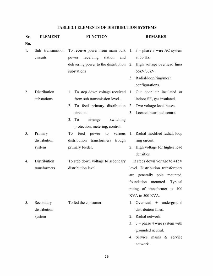
TABLE 2.1 ELEMENTS OF DISTRIBUTION SYSTEMS
Sr.
No.
ELEMENT FUNCTION REMARKS
1. Sub transmission
circuits
To receive power from main bulk
power receiving station and
delivering power to the distribution
substations
1. 3 – phase 3 wire AC system
at 50 Hz.
2. High voltage overhead lines
66kV/33kV.
3. Radial/loop/ring/mesh
configurations.
2. Distribution
substations
1. To step down voltage received
from sub transmission level.
2. To feed primary distribution
circuits.
3. To arrange switching
protection, metering, control.
1. Out door air insulated or
indoor SF6 gas insulated.
2. Two voltage level buses.
3. Located near load centre.
3. Primary
distribution
system
To feed power to various
distribution transformers trough
primary feeder.
1. Radial modified radial, loop
ring circuit.
2. High voltage for higher load
densities.
4. Distribution
transformers
To step down voltage to secondary
distribution level.
It steps down voltage to 415V
level. Distribution transformers
are generally pole mounted,
foundation mounted. Typical
rating of transformer is 100
KVA to 500 KVA.
5. Secondary
distribution
system
To fed the consumer 1. Overhead + underground
distribution lines.
2. Radial network.
3. 3 – phase 4 wire system with
grounded neutral.
4. Service mains & service
network.

30
2.8 A.C. Distribution System
Nowadays electrical energy is generated, transmitted and distributed in the form of alternating
current. One important reason for the widespread use of alternating current in preference to
direct current is the fact that alternating voltage can be conveniently changed in magnitude by
means of a transformer. Transformer has made it possible to transmit a.c. power at high voltage
and utilize it at a safe potential. High transmission and distribution voltages have greatly reduced
the current in the conductors and the resulting line losses.
There is no definite line between transmission and distribution according to voltage or bulk
capacity. However, the down sub-station is fed by the transmission system and the consumers’
meters. The a.c. distribution system is classified into (i) primary distribution system and (ii)
secondary distribution system.
(i) Primary Distribution System: It is part of a.c. distribution system, which operates a voltages
somewhat higher than general utilization and handles large blocks of electrical energy than the
average low-voltage consumer uses.
Figure 2.2 Primary Distribution Systems.
The voltage used for primary distribution depends upon the amount of power to be conveyed and
the distance of the sub-station required to be fed. The most commonly used primary distribution
voltages are 22 kV, 6.6 kV and 2.2 kV. Due to economic considerations, primary distribution is
carried out by 3-phase, 3-wire system. Figure 2.2 shows a typical primary distribution system.
Electric power from the generating station is transmitted at high voltage to the sub-station

31
located in or near the city. At this sub-station, voltage is stepped down to 11kV with the help of
step-down transformer. Power is supplied to various sub-stations for distribution or to big
consumers at this voltage. This forms the high voltage distribution or primary distribution.
(ii) Secondary Distribution System: It is that part of a.c. distribution system that includes the
range of voltages at which the ultimate consumer utilizes the electrical energy delivered to him.
The secondary distribution employs 400/230 V, 3-phase, 4-wire system. Figure 2.3 shows a
typical secondary distribution system.
Figure 2.3 Secondary Distribution Systems.
The primary distribution circuit delivers power to various sub-stations, called distribution sub-
stations. The sub-stations are situated near the consumer’s localities and contain step-down
transformers. At each distribution sub-station, the voltage is stepped down to 400 V and power is
delivered by 3-phase, 4-wire a.c. system. The voltage between any two phases in 400 V and
between any phase and neutral is 230. The single phase domestic loads are connected between
any one phase and the neutral whereas 3-phase 400 V motor loads are connected across 3-phase
lines directly.

32
2.9 Direct Current System
Direct current systems usually consist of two or three wires. Although such distribution systems
are no longer employed, except in very special instances, older ones now exist and will continue
to exist for some time. Direct current systems are essentially the same as single- phase ac
systems of two or three wires; the same discussion for those systems also applies to dc systems.
2.10 Over Head versus Underground System
The distribution system can be overhead or underground. Overhead lines are generally
mounted on wooden, concrete or steel poles which are arranged to carry distribution
transformers in addition to the conductors. The choice between overhead and underground
system depends upon a number of widely differing factors.
1. Public Safety:- The underground system is more safe than overhead system because all
distribution wiring is placed underground and there are little chances of any hazard.
2. Initial Cost:- The underground system is more expensive due to the high cost of trenching,
conduits, cables, manholes, and other special equipments. The initial cost of an underground
system may be five to ten times than that of an overhead system.
3. Flexibility:- The overhead system is much more flexible than the underground system. In the
latter case, manholes, duct lines etc., are permanently placed once installed and the load
expansion can only be met by laying new lines. However on an overhead system, poles, wires,
transformer etc., can be easily shifted to meet the change in load conditions.
4. Faults:- The chances of fault in underground system are very rare as the cables are laid
underground and are generally provided with better insulation.
5. Appearance:- The general appearance of an underground system is better as all the
distribution lines are visible. This factor is exerting considerable public pressure on electric
supply companies to switch over to underground system.
6. Fault location and repairs:- In general, there are little chances of fault in an underground
system. However, if a fault does occur, it is difficult to locate and repair the system. On an
overhead system, the conductors are visible and easily accessible so that fault locations and
repairs can easily be made.

33
7. Current carrying capacity and voltage drop:- An overhead distribution conductor has a
considerably higher current carrying capacity than an underground cable conductor of the same
material and cross-section. On the other hand, underground cable conductor has much lower
inductive reactance than that of an overhead conductor because of closer spacing of conductor.
8. Useful Life:- The useful life of underground system is much longer than that of an overhead
system. An overhead system may have a useful life of 25 years, whereas an underground system
may have a useful life of more than 50 years.
9. Maintenance cost:- The maintenance cost of underground system is very low as compared
with that of overhead system because of less chances of fault and service interruptions from
wind, ice, lightning as well as from traffic hazards.
10. Interference with communication circuits:- An overhead system causes electromagnetic
interference with telephone lines. The power line currents are superimposed on speech currents,
resulting in the potential of the communication channel being raised to an undesirable level.
However, there is no such interference with the underground system.
2.11 Connection Scheme of Distribution System
All distribution of electrical energy is done by constant voltage system. In practice, the following
distribution circuits are generally used. According to connection scheme the distribution system
has three types as given below:
(i) Radial System.
(ii) Ring Main System.
(iii)Interconnected system.

34
2.12 Radial Distribution System
A radial system has only one power source for a group of customers. A power failure, short-
circuit, or a downed power line would interrupt power in the entire line which must be fixed
before power can be restored. The figure of Radial Distribution System is shown as :-
Figure 2.4 Radial Distribution System
In this system, separate feeders radiate from a single sub-station and feed the distributors at one
end only. Figure 2.5 (a) shows a single line diagram of a radial system for d.c. Distribution
where a feeder OC supplies a distributor AB at point A. Obviously, the distributors are fed at one
point only i.e. point A in this case. Figure 2.5 (b) shows a single line diagram of radial system for
a.c. distribution. The radial system is employed only when power is generated at low voltage and
the sub-station is located at the centre of load. This is the simplest distribution circuit and has the
lowest initial cost.
Figure 2.5 Single Line Diagram of Radial Distribution System
35
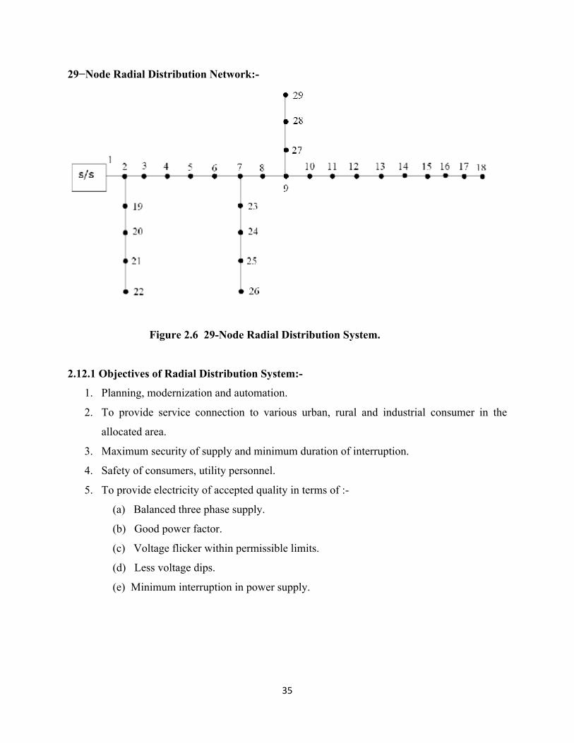
29−Node Radial Distribution Network:-
Figure 2.6 29-Node Radial Distribution System.
2.12.1 Objectives of Radial Distribution System:-
1. Planning, modernization and automation.
2. To provide service connection to various urban, rural and industrial consumer in the
allocated area.
3. Maximum security of supply and minimum duration of interruption.
4. Safety of consumers, utility personnel.
5. To provide electricity of accepted quality in terms of :-
(a) Balanced three phase supply.
(b) Good power factor.
(c) Voltage flicker within permissible limits.
(d) Less voltage dips.
(e) Minimum interruption in power supply.
36
2.12.2 Advantages of Radial Distribution System:-
(a) Radial distribution system is easiest and cheapest to build.
(b) The maintenance is easy.
(c) It is widely used in sparsely populated areas.
2.12.3 Drawback of Radial Distribution System:-
(a) The end of the distributor nearest to the feeding point will be heavily loaded.
(b) The consumers are dependent on a single feeder and single distributor. Therefore, any
fault on the feeder or distributor cuts off supply to the consumers who are on the side of
the fault away from the sub-station.
(c) The consumers at the distant end of the distributor would be subjected to serious voltage
fluctuations when the load on the distributor changes.
37
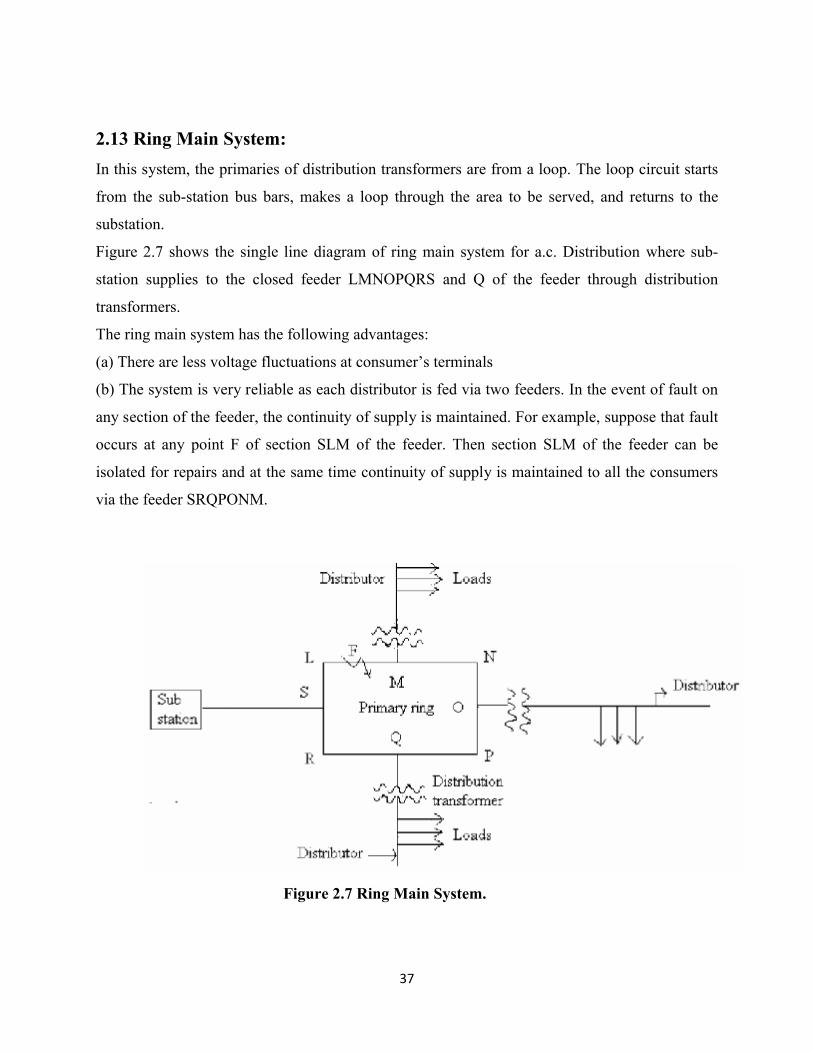
2.13 Ring Main System:
In this system, the primaries of distribution transformers are from a loop. The loop circuit starts
from the sub-station bus bars, makes a loop through the area to be served, and returns to the
substation.
Figure 2.7 shows the single line diagram of ring main system for a.c. Distribution where sub-
station supplies to the closed feeder LMNOPQRS and Q of the feeder through distribution
transformers.
The ring main system has the following advantages:
(a) There are less voltage fluctuations at consumer’s terminals
(b) The system is very reliable as each distributor is fed via two feeders. In the event of fault on
any section of the feeder, the continuity of supply is maintained. For example, suppose that fault
occurs at any point F of section SLM of the feeder. Then section SLM of the feeder can be
isolated for repairs and at the same time continuity of supply is maintained to all the consumers
via the feeder SRQPONM.
Figure 2.7 Ring Main System.

38
2.14 Interconnected System:
When the feeder ring is energized by two or more than two generating stations or sub stations, it
is called interconnected system. Figure 2.8 shows the single line diagram of interconnected
system where the closed feeder ring ABCD is supplied by two sub-stations S1 and S2 at points D
and C respectively. Distributors are connected to points O, P, Q and R of the feeder ring through
distribution transformers.
The interconnected system has the following advantages:
(a) It increases the service reliability.
(b) Any area fed from one generating station during peak load hours can be fed from the other
generating station. This reduces reserve power capacity and increases efficiency of the system.
The figure for the interconnected distribution system is given following as 2.8
Figure 2.8 Interconnected System.

39
CHAPTER-3
LOAD FLOW
3.1 Power Flow Analysis
The electric power system is one of the tools for converting and transporting energy, which is
playing an important role in meeting the challenges of modern life.
Planning the operation, looking out for a scope of expansion in future, all require a proper load
flow study of the system, transient behavior of the system as well as correct analysis of fault and
methods to mitigate the effects of the same.
Load flow analysis aims at determination of system parameters like voltage, current, power
factor power (real and reactive) flow at various points in the electric system under existing
conditions of normal operation. This analysis helps in determining the scope of future expansion
of the system.
In power system powers are known rather than currents. Thus the resulting equations in terms of
power, known as power flow equation, become non linear and must be solved by iterative
techniques. Power flows studies, commonly referred to as load flow, are the backbone of power
system analysis and design. They are necessary for planning, operation, economic scheduling
and exchange of power between utilities. In addition, power flow analysis is required for many
other analyses such as transient stability and contingency studies.
The two primary considerations in the development of an effective engineering computer
program are:
(1) The formulation of a mathematical description of the problem; and
(2) The application of a numerical method for a solution.
The analysis of the problem must also consider the interrelation between these two factors. The
mathematical formulation of the problem results in a system of algebraic nonlinear equations.
The load flow problem consists of calculation of power flow and voltages of a network for
specified terminal or bus conditions. A single phase representation is adequate since power
systems are usually balanced. First the power and load shared by each of the generators is
calculated during the course of normal operation. Then the effect on bus system on changing the
load requirement will be seen.

40
The power flow analysis is a very important and fundamental tool in power system analysis.
Power flow analysis plays the major role during the operational stages of any system for its
control and economic schedule, as well as during expansion and design stages. The purpose of
any load flow analysis is to compute precise steady-state voltages and voltage angles of all buses
in the network, the real and reactive power flows into every line and transformer, under the
assumption of known generation and load.
Successful operation of electrical systems requires that :-
a. Generation must supply the demand (load) plus the losses.
b. Bus voltage magnitudes must remain close to rated values.
c. Generators must operate within specified real and reactive power limits.
d. Transmission lines and transformers should not be overloaded for long periods.
The voltages and power flows in an electrical system can be determined for a given set of
loading and operating conditions. This is known as the power flow problem. Power flow analysis
is used extensively in the planning, design and operation of electrical systems.
In power flow analysis, it is normal to assume that the system is balanced and that the network is
composed of constant, linear, lumped-parameter branches. (In the most basic form of the power
flow, transformer taps are assumed to be fixed. This assumption is relaxed in commercial power
flows though.). Therefore nodal analysis is generally used to describe the network. However,
because the injection/demand at bus-bars is generally specified in terms of real and reactive
power, the overall problem is nonlinear. Accordingly, the power flow problem is a set of
simultaneous nonlinear algebraic equations. Numerical techniques are required to solve this set
of equations.

41
3.2 Need of Load Flow Study
Load flow study in power system is the steady state solution of power system network .The
power system is modeled by an electric network and solve for steady state power and voltage at
various buses .The direct analysis of circuits is not possible as the loads are given in terms of
complex powers rather than impedances and the generators behaves more like power source than
voltage source.
3.3 Significance of Load Flow Study
1. Determination of current, voltage, active power, reactive power etc. at various buses in power
system operating under normal steady state or static condition.
2. To plan best operation and control of existing system.
3. To plan future expansion to keep pace with load growth.
4. Help in ascertaining the effect of new load, new generating stations, new lines and new
interconnections before they are installed.
5. Due to this information system losses are minimized and also check is provided on system
stability.
6. Provides the proper prefault power system analysis to avoid system outage due to fault.
3.4 Information Obtained from Load flow Studies
1. Magnitude of voltages (Vi) .
2. Phase angle of voltages (δi) .
3. Active power (Pi) .
4. Reactive power (Qi)
3.5 Methods Used to Solve Static Load Flow Equations
It is important to note that the voltages and power flows in an electrical system can be
determined for a given set of loading and operating conditions. This is known as the power flow
problem. Power flow analysis is used extensively in the planning, design and operation of
,electrical systems.

42
The solution of static load flow equation is difficult because of non linear characteristics of
equations as bus voltages are involved in product form and sine, cosine terms are present. Hence
solutions are possible through only iterative numerical techniques.
Following methods are used to solve static load flow equation:
1. GAUSS-SEIDEL METHOD.
2. NEWTON RAPHSON METHOD.
3. FAST DECOUPLE METHOD.
3.5.1 The Advantages of These Methods used in Distribution System are
a) They should have high speed and low storage requirements, especially for real-time large
system applications, as well as multiple case and interactive applications.
b) They should be highly reliable, especially for ill-conditioned problems, outage studies,
and real-time applications.
c) They should have acceptable versatility and simplicity.
3.6 Constraints at Nodes
Four variables are associated with each node:-
a. Bus voltage magnitude (V ).
b. Voltage angle (θ).
c. Real power (P).
d. Reactive power (Q).
Each node introduces two equations, namely the real and reactive power balance equations. To
obtain (isolated) solutions for a set of simultaneous equations, it is necessary to have the same
number of equations as unknowns. Therefore two of the variables associated with each bus must
be specified, i.e., given fixed values. The other two variables are free to vary during the solution
process.
The traditional way of specifying bus-bar quantities allows buses to be identified as follows:-

43
3.6.1 PQ Bus-bar:- At which the net active and reactive powers are specified. The net power
entering a bus-bar is the power supplied to the system from a generating source minus the power
consumed by a load at that bus-bar.
3.6.2 PV Bus-bar:- At which the net active power is specified, and the voltage magnitude is
specified.
The net reactive power is an unknown which is determined as part of the power flow solution.
This type of bus-bar typically represents a node in the system at which a synchronous source
(generator or compensator) is connected, where the source’s reactive power output is varied to
control the voltage magnitude to a scheduled value.
3.6.3 Slack or Swing Bus-bar:- Where the voltage magnitude and angle are specified.
Generally the angle is set to zero. Unlike the other two bus types, which represent physical
system conditions, this bus-bar type is more a mathematical requirement. It is needed to provide
a ‘reference’ angle to which all other angles are referred. Also, this bus absorbs any real power
mismatch across the system. (Note that it is not possible to specify the net active power at all
buses in the system, because transmission losses are unknown until the power flow solution is
completed.) Normally there can only be one slack bus-bar in the system. It is generally chosen
from among the voltage controlled bus-bars.
3.7 Choice of Variables
Basically load-flow analysis deals with known real and reactive power flows at each bus, and
those voltage magnitudes that are explicitly known, and from this information calculating the
remaining voltage magnitudes and all the voltage angles. We are familiar with the notion of
organizing the descriptive variables of the circuit into categories of “knowns” and “unknowns,”
whose relationships can subsequently be expressed in terms of multiple equations.
For AC circuits, because we have introduced the dimension of time: unlike in DC, where
everything is essentially static (except for the instant at which a switch is thrown), with AC we
are describing an ongoing oscillation or movement. Thus each of the two main variables, voltage
and current, in an AC circuit really has two numerical components: a magnitude component and
a time component. By convention, AC voltage and current magnitude are described in terms of

44
root-mean-squared (r.m.s.) values and their timing in terms of a phase angle, which represents
the shift of the wave with respect to a reference point in time . To fully describe the voltage at
any given node in an AC circuit, we must, therefore, specify two numbers: a voltage magnitude
and a voltage angle. Accordingly, when we solve for the currents in each branch, we will again
obtain two numbers: a current magnitude and a current angle.
When we consider the amount of power transferred at any point of an AC circuit, we again have
two numbers: a real and a reactive component. An AC circuit thus requires exactly two pieces of
information per node in order to be completely determined. More than two, and they are either
redundant or contradictory; fewer than two and possibilities are left open so that the system
cannot be solved. Owing to the nonlinear nature of the load-flow problem, it may be impossible
to find one unique solution because more than one answer is mathematically consistent with the
given configuration. However, it is usually straightforward in such cases to identify the “true”
solution among the mathematical possibilities based on physical plausibility and common sense.
Conversely, there may be no solution at all because the given information was hypothetical and
does not correspond to any situation that is physically possible. Still, it is true in principle—and
most important for a general conceptual understanding that two variables per node are needed to
determine everything that is happening in the system. In practice, current is not known at all; the
currents through the various circuit branches turn out to be the last thing that we calculate once
we have completed the load-flow analysis. Voltage, as we will see, is known explicitly for some
buses but not for others. More typically, what is known is the amount of power going into or out
of a bus.
Load-flow analysis consists of taking all the known real and reactive power flows at each bus,
and those voltage magnitudes that are explicitly known, and from this information calculating the
remaining voltage magnitudes and all the voltage angles. This is the hard part. The easy part,
finally, is to calculate the current magnitudes and angles from the voltages. We know how to
calculate real and reactive power from voltage and current: power is basically the product of
voltage and current, and the relative phase angle between voltage and current determines the
respective contributions of real and reactive power. Conversely, one can deduce voltage or
current magnitude and angle if real and reactive power are given, but it is far more difficult to
work out mathematically in this direction. This is because each value of real and reactive power
would be consistent with many different possible combinations of voltages and currents. In order
45
to choose the correct ones, we have to check each node in relation to its neighboring nodes in the
circuit and find a set of voltages and currents that are consistent all the way around the system.
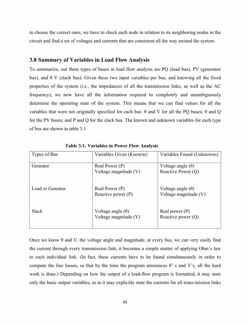
3.8 Summary of Variables in Load Flow Analysis
To summarize, our three types of buses in load flow analysis are PQ (load bus), PV (generator
bus), and θ V (slack bus). Given these two input variables per bus, and knowing all the fixed
properties of the system (i.e., the impedances of all the transmission links, as well as the AC
frequency), we now have all the information required to completely and unambiguously
determine the operating state of the system. This means that we can find values for all the
variables that were not originally specified for each bus: θ and V for all the PQ buses; θ and Q
for the PV buses; and P and Q for the slack bus. The known and unknown variables for each type
of bus are shown in table 3.1
Table 3.1: Variables in Power Flow Analysis
Types of Bus Variables Given (Knowns) Variables Found (Unknowns)
Genrator
Load or Genrator
Slack
Real Power (P)Voltage magnitude (V)
Real Power (P)Reactive power (P)
Voltage angle (θ)Voltage magnitude (V)
Voltage angle (θ)Reactive Power (Q)
Voltage angle (θ)Voltage magnitude (V)
Real power (P)Reactive power (Q)
Once we know θ and V, the voltage angle and magnitude, at every bus, we can very easily find
the current through every transmission link; it becomes a simple matter of applying Ohm’s law
to each individual link. (In fact, these currents have to be found simultaneously in order to
compute the line losses, so that by the time the program announces θ’ s and V’s, all the hard
work is done.) Depending on how the output of a load-flow program is formatted, it may state
only the basic output variables, as in it may explicitly state the currents for all trans-mission links

46
in amperes; or it may express the flow on each transmission link in terms of an amount of real
and reactive power owing, in megawatts (MW) and (MVAr).
3.9 Power Flow Solution
Power flow studies ,commonly known as load flow ,form an important part of power system
analysis .They are necessary for planning ,economic rescheduling ,and control of existing system
as well as planning its future expansion .The problem consists of determining the magnitudes
and phase angle of voltages at each bus and active and reactive power flow in each line .
In solving a power flow problem, the system is assumed to be operating under balanced
conditions and a single phase model is used .Four quantities are associated with each bus.
These are voltage magnitude │V│, phase angle δ, real power P, and reactive power Q. The
system buses are generally classified into three types.
Slack bus one bus, known as slack or swing bus, is taken as reference where the magnitude and
phase angle of the voltage are specified. This bus makes up the difference between the scheduled
loads and the generated power that are caused by losses in the network.
Load buses at these buses the active and reactive powers are specified. The magnitude and phase
angle of the bus voltages are unknown. These buses are called P-Q buses.
Regulated buses these buses are the generator buses. They are also known as voltage-controlled
buses. At these buses, the real power and voltage magnitude are specified. The phase angles of
the voltage and reactive power are to be determined. The limits on the value of reactive power
are also specified. These buses are called P-V buses.

47
CHAPTER-4
ROLE OF POWER FLOW IN DISTRIBUTION SYSTEM
4.1 Introduction
Load flow analysis forms an essential prerequisite for power system studies. Considerable
research has already been carried out in the development of computer programs for load flow
analysis of large power systems. However, these general purpose programs may encounter
convergence difficulties when a radial distribution system with a large number of buses is to be
solved and, hence, development of a special program for radial distribution studies becomes
necessary.
There are many solution techniques for load flow analysis. The solution procedures and
formulations can be precise or approximate, with values adjusted or unadjusted, intended for
either on-line or off-line application, and designed for either single-case or multiple-case
applications.
Power flow method is a fundamental tool in application software for distribution management
system. In the past decades, a mass of methods to solve the distribution power flow problem
have been developed and well documented. These methods can be roughly categorized as node
based methods and branch based methods.
The first category used node voltages or currents injection as state variables to solve power flow
problem. In this category, the most notable methods include network equivalence method, Z-bus
method, Newton–Raphson’s algorithm, Fast Decoupled algorithm. The second category adopted
branch currents or branch powers as state variables to solve power flow problem. The
backward/forward sweep based methods and loop impedance methods can be categorized in this
group.
We are discussing here the Newton Raphson’s method and the Fast Decoupled Load Flow
method for the distribution system. The Fast Decoupled method is the modified version of
Newton Raphson’s method.

48
4.2 General Purpose Newton Raphson’s Method of Power flow Analysis
In solving a power flow problem, system is assumed to be operating under balanced conditions
and a single phase model is used. Four quantities are associated with each bus. These are voltage
magnitude |V|, phase angle δ, real power P, and reactive power Q.
The system buses are generally classified into three types:
Newton Raphson method is used for solving non linear algebraic equations. This method is
successive approximation procedure based on initial estimate of unknown and use of Taylor
series.
4.2.1 Power flow equation
Typical bus of a power system network shown in figure 4.1 as:
Figure 4.1 Typical bus of a power system network.
Applying kcl at this node
Ii = (y
i0+y
i1+y
i2+…y
in) Vi-y
i1V
1-y
i2V
2-… -y
inV
n … ..………...…(1)
where j≠I ….………… (2)
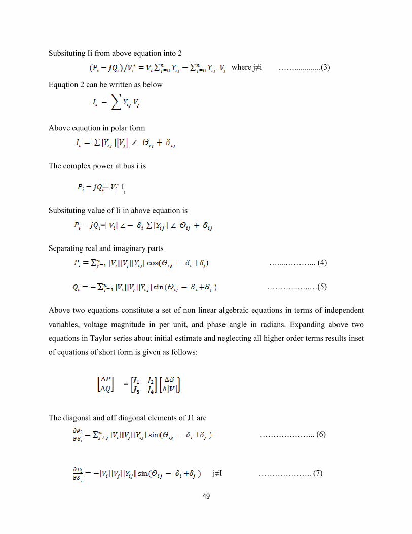
49
Subsituting Ii from above equation into 2
where j≠i …….............(3)
Equqtion 2 can be written as below
Above equqtion in polar form
The complex power at bus i is
= Ii
Subsituting value of Ii in above equation is
=|
Separating real and imaginary parts
) …....………... (4)
………...…..…(5)
Above two equations constitute a set of non linear algebraic equations in terms of independent
variables, voltage magnitude in per unit, and phase angle in radians. Expanding above two
equations in Taylor series about initial estimate and neglecting all higher order terms results inset
of equations of short form is given as follows:
=
The diagonal and off diagonal elements of J1 are
………………... (6)
j≠I ……………….. (7)

50
The diagonal and off diagonal of J4 are
= -2 - ……...........(8)
= - ………………(9)
The terms ΔPi(k) and ΔQi(k) are the differences between the scheduled and calculated
values,termed as power residuals, given by
ΔPi(k) = Pi(sch) -- Pi(k) ……………….(10)
ΔQi(k) = Qi(sch) - Qi(k) .…………........(11)
The new estimates for bus voltages are
δi(k+1) =δi(k) + Δδi(k) ………….........(12)
|Vi(k+1)| = |Vi(k)| + Δ|Vi(k)| ……………….(13)
4.2.2 Algorithm for Newton Raphson method of Load Flow Analysis
The procedure for power flow solution by the Newton-Raphson method is as follows:
1. For load buses , where Pi(sch) and Qi(sch) are specified, voltage magnitudes and phase
angles are set equal to the slack bus values , or 1.0 and 0.0, i.e., |Vi(0)| = 1.0 and δi(0) =
0.0. For voltage-regulated buses, where |Vi| and Pi(sch) are specified, phase angles are set
equal to the slack bus angle, or 0, i.e., δi(0) = 0.
2. For load buses, Pi(k) and Qi
(k) are calculated from (4)and (5)and ΔPi(k) and ΔQi
(k) are
calculated (10) and (11).
3. For voltage-controlled buses, Pi(k) and ΔPi
(k) are calculated from (4) and (10), respectively.
4. The elements of the Jacobian matrix (J1,J2,J3 and J4) are calculated from (6)- (8).
5. The linear simultaneous equation is solved directly by optimally ordered triangular
factorization and Gaussian elimination.

51
6. The new voltage magnitudes and phase angles are computed from (12) and (13).
7. The process is continued until the residuals ΔPi(k) and ΔQi
(k) are less than the specified
accuracy i.e.,
| ΔPi(k)| <= ε
| ΔQi(k)| <= ε
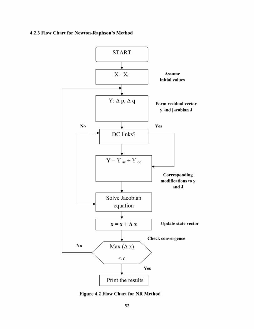
52
4.2.3 Flow Chart for Newton-Raphson’s Method
Figure 4.2 Flow Chart for NR Method
START
X= X0
Y: Δ p, Δ q
Y = Y ac + Y dc
Solve Jacobian equation
x = x + Δ x
Print the results
Max (Δ x)
< ε
DC links?
Assume initial values
Form residual vector y and jacobian J
No Yes
Corresponding modifications to y
and J
Update state vector
No
Yes
Check convergence

53
4.3 General purpose Fast Decoupled Power Flow Method
Probably almost all the relevant known numerical methods used for solving the nonlinear
equations have been applied in developing power flow models. Among various methods, power
flow models based on the Newton- Raphson (NR) method have been found to be most reliable.
Many decoupled polar versions of the NR method have been attempted for reducing the memory
requirement and computation time involved for power flow solution. Among decoupled versions,
the fast decoupled load flow (FDLF) model developed by Stott and Alsac is possibly the most
popular of those frequently used by the power utilities.
The basic equations used in FDLF methods are given below:-
'B
V
P…………………(14)
And
VBV
Q
" …………………(15)
Where [ B ] = -ve imaginary elements of Ybus matrix.
While forming the above model, certain additional assumptions have been made to improve the
convergence property of the FDLF model, they are:-
a) While forming [B’], parameters such as shunt reactance and off-nominal in-phase
transformer taps are omitted.
b) Line series resistances are neglected while forming [B’].
These additional assumptions have a significant effect on the convergence property of the FDLF
model.
In view of the above, another motivating factor is to develop an efficient but simple
compensation technique to handle the problems of Q-limit enforcements at PV buses associated
with bus-type switching. Therefore, in the proposed work, attention is focused on two aspects:-

54
a) To develop a FDPF model which exhibits stable convergence behavior for both normal
and ill-conditioned situations and to compare its performance with that of the Stott FDLF
model.
b) To develop an efficient compensation technique for Q-limit enforcement problems at PV
buses to contain the number of iterations taken so that they are comparable with the
number of iterations taken for the unadjusted solution case.
4.3.1 Mathematical Model of Fast Decoupled Power Flow Method
In a power system network, the net injected active and reactive powers at an ith bus are given
by:-
NB
lijijijijjii BGVVP
1
sincos …………………(16)
And
NB
Jijijijijjii BGVVQ
1
coscos .............................(17).
where Vi and Vj , voltage magnitudes at the ith and jth buses, respectively; Gij + jBij is the ijth
element of the Y-bus; and NB, total number of buses. The linearised power flow eqns. 16 and
17 are expressed in compact form as:-
VJJ
JJ
Q
P 43
21 ...............................(18)
In eqn. 18, the sub matrices J1 and J4 have dissimilar dimensions due to the absence of the Q-V
equations of PV buses. The following assumptions are made in shaping the FDPF model from
eqn. 18:-
(i) The sub matrices J2 and J3 are ignored.
(ii) All network shunt reactance such as line charging reactance, external reactance located at
buses and shunts formed due to representation of off-nominal in-phase transformers are lumped

55
at each bus and are treated as constant impedance loads. Hence, the Y-bus elements (diagonals)
are devoid of these shunts. By involving the second assumption, the number of parameters
involved will be reduced while forming [B’] and [B”] matrices and attention can be focused on
line series resistances to study their effect on the convergence behavior of the FDPF model. The
effect of phase shifters is not studied in the present model. All buses are assumed to be of the PQ
type while forming the Jacobean-like matrices [B’] and [B”] with a flat voltage start of 1.0 p.u.
After incorporating the above assumptions, the resulting FDPF equations are:-
'
'B
V
P .........................(19)
And
VBV
Q
"
' ………...........(20)
Where
1,1,,'
shuntscaloulatedtscheduledi PPPP
ishuntstcalculatedfscheduledi QQQQ ,,,' ……………....(21)
The suffix i stands for the ith bus. Pshunts,i ; Qshunts,i are the real and reactive powers, respectively,
due to lumped shunts at the ith bus. It should be. noted that the dimensions of the Jacobians [ B’ ]
and [ B’’] are the same, (NB - 1) by (NB - 1) in eqns. (19) and (20) whereas that of [ B”] in eqn.
15 is (NB - MB - 1) by (NB - MB - 1) where, MB is the number of voltage controlled buses.
When both [ B’] and [ B”] are of the same order of (NB - 1). These matrices are real, sparse and
only contain network elements. These matrices are only factorised once, then stored and are held
constant throughout the solution process. The solution of eqns. 22 and 23 are given by:-
V
PB
'' 1 ……...............(22)
And
V
QBV
'" 1 ...….................(23)
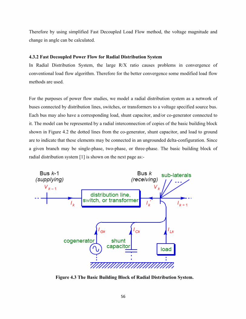
56
Therefore by using simplified Fast Decoupled Load Flow method, the voltage magnitude and
change in angle can be calculated.
4.3.2 Fast Decoupled Power Flow for Radial Distribution System
In Radial Distribution System, the large R/X ratio causes problems in convergence of
conventional load flow algorithm. Therefore for the better convergence some modified load flow
methods are used.
For the purposes of power flow studies, we model a radial distribution system as a network of
buses connected by distribution lines, switches, or transformers to a voltage specified source bus.
Each bus may also have a corresponding load, shunt capacitor, and/or co-generator connected to
it. The model can be represented by a radial interconnection of copies of the basic building block
shown in Figure 4.2 the dotted lines from the co-generator, shunt capacitor, and load to ground
are to indicate that these elements may be connected in an ungrounded delta-configuration. Since
a given branch may be single-phase, two-phase, or three-phase. The basic building block of
radial distribution system [1] is shown on the next page as:-
Figure 4.3 The Basic Building Block of Radial Distribution System.

57
One of the key concepts behind our formulation is that the voltage and current at one bus can be
expressed as a function of the voltage and current at the next bus. If we let the equations [1] as
1k
kk I
VW ..........................(24).
The branch update function [1] is given below as:
kkk wgW 1 ….......................(25).
Where Wk is a vector containing the real and imaginary parts of the voltages and currents at bus
k. The function gk is determined by the sub-laterals attached at bus k as well as the models for
distribution lines, switches, transformers, loads, shunt capacitors, and co-generators. From Vk we
can compute the currents injected by the loads, shunt capacitors, and co-generators. Given Ik + 1
and the currents Ij injected into sub-laterals branching off from bus k, we apply KCL at bus k to
caculate current [1] given as:-
KAJ
jkLKCKGKk IIIIII 1' …….…............(26).
Where Ak is the set of buses adjacent to bus k on sub-laterals.
From the following equation (28), we can solve for the voltage and current at the primary given
the voltage and current at the secondary [1] as:-
k
k
ssk
spk
psk
ppk
K
K
V
V
YY
YY
I
I 1
' …………………(27).
Therefore by solving equation (27) , we get
kss
kksp
kk VYIYV
'1
1 ..........................(28).
And
kps
kkpp
kk VYVYI 1 ..........................(29).
So that by using this method we get the converged value easily and fast than the other ordinary
methods.

58
4.4 Algorithm for Fast Decoupled Power Flow Method
The stepwise algorithm to solve the power flow problem by using Fast Decoupled Power Flow
Method is given below as:-
Step 1: Creation of the bus admittance Ybus according to the lines data given by the IEEE
standard bus test systems.
Step 2: Detection of all kinds and numbers of buses according to the bus data given by the IEEE
standard bus test systems, setting all bus voltages to an initial value of 1 pu, all voltage angles to
0, and the iteration counter iteration to 0.
Step 3: Creation of the matrices B' and B" according to equations (30) and (31) as given below:-
'BVi
P...........................(30).
And
VBVi
Q
" ...........................(31).
Where B' and B" are the imaginary part of the bus admittance matrix Ybus
, such that B’ contains
all buses admittances except those related to the slack bus, and B" is B' deprived from all
voltage-controlled buses related admittances.
Step 4: Calculate the value of ΔP and ΔQ by using the following equations as
HP ........................(32).
And
VLQ .........................(33).
Step 5: Check the convergence as
Now if max(ΔP, ΔQ) ≤ accuracy
then Go to Step 6.
59
Else
(a). Calculation of the H and L elements from the following equqtions as given:-
iiiii BVH .............................(34).
And
ijiij BVH .............................(35).
Similarly, the diagonal elements of the L matrix can be written as:-
iiiii BVL .............................(36).
And
ijiij BVL .............................(37).
(b). Calculation of the real and reactive power at each bus, and checking if Mvar of
generator buses are within the limits, otherwise update the voltage magnitude at these buses by
±2 %.
(c). Calculation of the power residuals, ΔP and ΔQ.
(d). Calculation of the bus voltage and voltage angle updated Δδ and ΔV according to
equations given below:-
V
PB
1' ......................(38).
And
V
QBV
1" .......................(39).
(e). Update of the voltage magnitude V and the voltage angle δ at each bus .

60
(f). The current can be calculated from the calculated Ybus and the calculated voltage as
given in the following equation as:-
k
k
ssk
spk
psk
ppk
k
k
V
V
YY
YY
I
I 1
'……...........(40).
(g). Increment of the iteration counter iter = iter + 1.
Step 6: if iter ≤ maximum number of iteration
Then Go to Step 4
Else Print out ‘Solution did not converge’ and go to Step 6.
Step 7: Print out of the power flow solution, computation and display of the line flow, current
and losses.
4.5 Advantages of Fast Decoupled Method:-
1. The memory requirement is very less than the other ordinary used method like as
Newton’s method, Gauss-Seidel method etc.
2. This method is less complicated than the other methods, therefore it is more easy method
to calculate the power flow.
3. The number of iteration and size of equations used is less.
4. The convergence is fast than the other method.
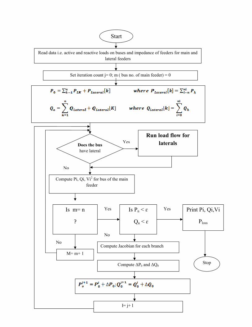
61
Read data i.e. active and reactive loads on buses and impedance of feeders for main and lateral feeders
Set iteration count j= 0; m ( bus no. of main feeder) = 0
Does the bushave lateral
Run load flow for laterals
Compute Pi, Qi, Vi2 for bus of the main feeder
Compute Jacobian for each branch
Compute ΔP0 and ΔQ0
I= j+ l
Print Pi, Qi,Vi
Ploss
Stop
M= m+ 1
Start
Is m= n
?
Is Pn < ɛ
Qn < ɛ
Yes
No
Yes Yes
No
No

62
CHAPTER-5
RESULTS AND DISCUSSION
5.1 Discussion
Load flow is very important and fundamental tool for the analysis of any power system and used
in the operational as well as planning stages. Certain application, particularly in distribution
automation and optimization of power system requires repeated load flow solution. In these
applications it is very important to solve the load flow problem as efficiently as possible.
So that there are different type of methods are used to solve the load flow problem. A new
method of power flow analysis for solving balanced and unbalanced radial distribution systems
has been developed and successfully implemented. First, the radial distribution system is
properly modeled and a set of power flow equations is derived. After that, the solution method is
developed for solving the power flow study. The validity of the results of radial distribution flow
has also been verified by comparing them with the existing methods of power flow analysis. The
proposed method offers a very attractive combination of advantages over the existing methods
including the Newton Raphson’s method and the Fast-Decoupled method in terms of convergent
characteristic, computation time, simplicity and memory storage requirements. These methods
are explained above. In addition, its performance was also found to be better than the other
recent methods of power flow analysis developed for distribution systems. A more accurate
prediction of the power system performance can also be obtained with the incorporation of static
load models in the power flow study. The constant-power load model gave the most conservative
results, with the lowest voltage profile and the highest load demand as opposed to the constant-
impedance load model. Hence, it can be seen that accurate modeling of the load is necessary for
a good distribution system design. The convergence analysis on this power flow method shows
that its convergence property is neither affected by the number of buses nor the R/X ratio of the
distribution system. However, the method would take longer to converge for very heavily loaded
systems as well as for systems whereby there are more than 5 levels of laterals. In addition, using
different load models also affect the convergence of the method. The more sensitive the load
models are to the bus voltage, the slower the rate of convergence.

63
Here we used Newton Raphson’s and Fast Decoupled Power Flow Methods to solve the power
flow problem for the given distribution system. The Newton Raphson’s and Fast Decoupled
power flow solution techniques and host of their derivatives have efficiently solved “well
behaved” power systems. By using these methods we are able to calculate the active power (P),
reactive power (Q), path-loss and voltage (V) for 10 bus system data and for 33 bus system data.
5.2 Results
The results by using the methods explained above for the distribution system are given in the
following tables as:-
Table 5.1 Results for 10 Bus Systems without Load Flow Solution
Bus No. Active Power Reactive Power Path loss Voltage
1 3.170300 1.163396 0.010894 1.000000
2 2.724629 0.928449 0.000923 0.993463
3 2.489705 0.807121 0.041338 0.988780
4 2.021367 0.633850 0.024990 0.966335
5 1.615377 0.171734 0.045392 0.952326
6 1.185985 -0.011342 0.011806 0.923624
7 0.987878 -0.047832 0.019017 0.914543
8 0.694861 -0.072903 0.022967 0.897525
9 0.437895 -0.116926 0.011449 0.870152
10 0.035446 -0.171110 0.000000 0.000000
Total Active Power = 15.3677
Total Reactive Power = 3.1951
Total Path loss = 0.1888
Here these results are calculated without using any load flow technique.
The result for the same 10 bus distribution system by using load flow technique is given below,
the load flow technique used here is the Newton Raphson and Fast Decoupled Power flow
method.
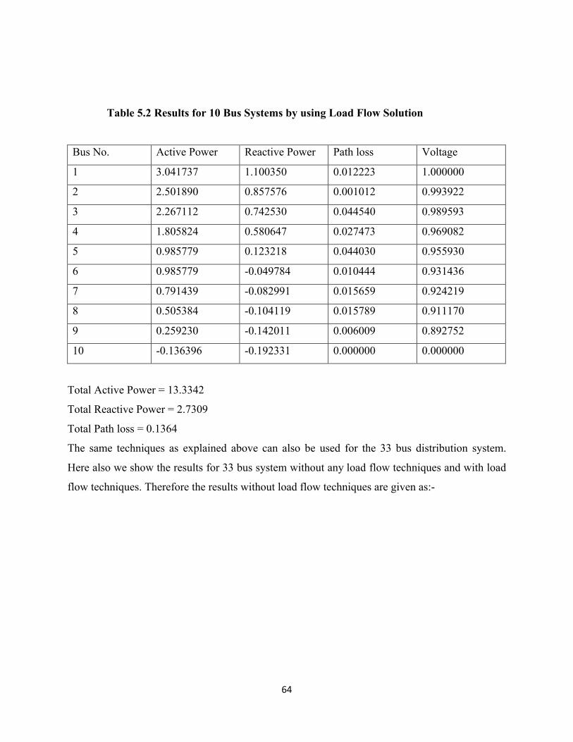
64
Table 5.2 Results for 10 Bus Systems by using Load Flow Solution
Bus No. Active Power Reactive Power Path loss Voltage
1 3.041737 1.100350 0.012223 1.000000
2 2.501890 0.857576 0.001012 0.993922
3 2.267112 0.742530 0.044540 0.989593
4 1.805824 0.580647 0.027473 0.969082
5 0.985779 0.123218 0.044030 0.955930
6 0.985779 -0.049784 0.010444 0.931436
7 0.791439 -0.082991 0.015659 0.924219
8 0.505384 -0.104119 0.015789 0.911170
9 0.259230 -0.142011 0.006009 0.892752
10 -0.136396 -0.192331 0.000000 0.000000
Total Active Power = 13.3342
Total Reactive Power = 2.7309
Total Path loss = 0.1364
The same techniques as explained above can also be used for the 33 bus distribution system.
Here also we show the results for 33 bus system without any load flow techniques and with load
flow techniques. Therefore the results without load flow techniques are given as:-

65
Table 5.3 Results for 33 Bus Systems without Load Flow Solution
Bus No. Active Power Reactive Power Path Loss Voltage
1 0.365649 0.251579 0.001090 1.000000
2 0.319410 0.200005 0.004399 0.997215
3 0.213011 0.165243 0.001711 0.984202
4 0.199300 0.159207 0.001624 0.976480
5 0.191676 0.151781 0.003249 0.969651
6 0.105427 0.090438 0.00249 0.952647
7 0.085179 0.079127 0.000253 0.947693
8 0.064926 0.063717 0.000602 0.939762
9 0.048323 0.052224 0.000379 0.932188
10 0.041944 0.045935 0.000055 0.926226
11 0.037388 0.042936 0.000089 0.925465
12 0.031300 0.033957 0.000229 0.924163
13 0.025071 0.024167 0.000049 0.918412
14 0.013023 0.018113 0.000022 0.916318
15 0.007001 0.011884 0.000011 0.915146
16 0.000990 0.002406 0.000001 0.914348
17 -0.005011 -0.006955 0.000004 0.913978
18 -0.014015 -0.010668 1.011000 0.914501
1 0.036078 0.031653 0.000024 0.997215
2 0.026976 0.021857 0.000114 0.996537
3 0.017862 0.010765 0.000011 0.992139
4 0.008851 0.004172 0.000004 0.991357
5 -0.000153 -0.000144 0.001210 0.990716
1 0.093823 0.025625 0.000270 0.984202
2 0.083730 0.017076 0.000425 0.981050
3 0.041305 0.006211 0.000102 0.975505
4 -0.000797 -0.000599 0.000024 0.972861

66
Bus No. Active Power Reactive Power Path loss Voltage
1 0.079049 0.049827 0.000127 0.952647
2 0.070887 0.047232 0.000148 0.951264
3 0.064754 0.039455 0.000436 0.949498
4 0.058363 0.029469 0.000245 0.942567
5 0.046143 0.022438 0.000095 0.938092
6 0.045057 0.015074 0.000155 0.936247
7 0.029918 0.005847 0.000020 0.932254
8 0.008900 0.001746 0.000002 0.931490
9 -0.001102 -0.000867 0.000256 0.931224
Total Active Power = 2.4291
Total Reactive Power = 1.6974
Total Path loss = 0.0161
Here the power is distributed as from bus number 1-18, 1-5, 1-4 and from 1-9 by using the
distribution system.

67
Table 5.4 Results for 33 bus system by using load flow techniques are given as
Bus No. Active Power Reactive Power Path loss Voltage
1 10.518657 5.550569 0.101456 1.000000
2 9.209444 2.637625 0.010492 0.980900
3 8.964952 2.100510 0.533791 0.968041
4 8.004162 1.131802 0.449411 0.895906
5 7.173750 0.301195 1.136312 0.841283
6 5.653438 -0.837834 0.461245 0.712067
7 5.005894 -1.266013 0.980040 0.665094
8 3.751854 -1.835428 2.041124 0.569145
9 1.476729 -3.023783 2.165726 0.469736
10 1.079997 -4.298044 0.000000 0.601050
11 1.027264 -4.475270 0.005980 0.622751
12 0.582284 -4.844129 0.325793 0.656977
13 0.022887 -5.450928 0.313005 0.723883
14 0.717118 -5.830173 0.909303 0.761072
15 0.593185 -7.083504 0.487651 0.861326
16 0.278466 -7.651796 1.151400 0.909909
17 1.059234 -8.330173 2.714102 0.992246
18 1.929167 -9.883589 3.069534 1.182474
19 1.365367 -11.647924 0.071023 1.370562
20 0.903344 -11.934320 0.088023 1.397348
21 0.595274 -12.284987 0.432832 1.438107
22 0.023442 -13.093120 0.411262 1.516891
23 0.621819 -13.532684 1.177840 1.559054
24 0.983021 -14.671304 0.550194 1.677413
25 0.051827 -15.589803 1.321855 1.729065
26 1.654028 -16.481829 3.147915 1.817563
27 1.680187 -18.292955 3.521232 2.011023

68
Bus No. Active Power Reactive Power Path loss Voltage
28 2.115045 -20.301507 0.599838 2.230037
29 1.281207 -21.104086 1.364194 2.308275
30 0.473987 -22.954771 3.194340 2.500890
31 2.994353 -24.983443 3.569614 2.735867
32 0.809261 -25.793499 3.215165 2.801830
33 2.796905 -27.664257 0.000000 0.000000
Total Active Power = 2.0135
Total Reactive Power = 1.396
Total Path loss = 0.0136
By comparing table 5.3 and table 5.4 it is clear that total path loss value is lower in table 5.4
which is obtained from results for 33 bus system by using load flow technique. Also, active
power is increased and reactive power is decreased by using load flow techniques which when
compared to results for 33 bus system without load flow solution.
69
CHAPTER-6
CONCLUSION AND FUTURE SCOPE
6.1 Conclusion
In this a new method of power flow analysis for solving unbalanced radial distribution systems
has been developed and successfully implemented. In this we have exploited the radial structure
(physical property) and the decoupling numerical property of a distribution system to develop a
fast decoupled Newton method for solving unbalanced distribution load flow. It involves a
reduced set of equations and unknowns proportional to the number of laterals in the network as
opposed to the number of buses. Due to the reduced number of equations and the fact that the
Jacobian is approximated by a constant triangular matrix, it is significantly faster than the
implicit Zbus Gauss method or the traditional Newton method based on Ybus. Since each function
evaluation involves updating each bus voltage and current and the Jacobian is triangular the
computation in each iteration is proportional to n, making it suitable for very large radial
systems. It is also shown to be more efficient than the backward/forward sweep method of due to
the savings during the update of the end voltages. The load flow method proposed in this paper
could possibly be improved further in several ways. As described here, it is limited to radial
systems with one voltage-regulated bus treated as the source. Therefore considerable saving in
the execution time has been achieved. The proposed model exhibits very reliable convergence
even for high degree of ill-conditioning, where traditional Newton’s method failed to converge.
The model will be very useful for reactive power planning and management studies on all sizes
of system with any degree of ill-conditioning. Effectiveness of the proposed method has been
tested by two examples 10-node and 33- node radial distribution networks. The voltage
convergence has assured the satisfactory convergence in all these cases. The superiority of the
proposed method in terms of speed has been checked by comparing with the other existing
methods. The proposed method consumes less amount of memory compared to other load flow
techniques.

70
The network is then solved using a radial load flow algorithm along with corrections to the
breakpoint currents or powers. These approaches also allow for PV buses, treated as artificial
breakpoints, making them suitable for weakly-meshed transmission systems.
6.2 Future Scope
(i) Due to some distinct characteristics of distribution system, conventional load flow algorithm
may fail to converse in solving to distribution network. Therefore various sweep based methods
can be used to study the power flow of distribution network. Backward/forward sweep algorithm
for three phase load flow analysis of radial distribution can be used.
(ii) The Jacobian matrix used to solve the load flow problem is a time consuming system and the
memory requirement is more. The Fast Decoupled Power Flow has less memory requirement and
it is easy to operate. So that in future the use of Fast Decoupled Power Flow method to solve the
power flow in distribution and transmission system is best.

71
REFERENCES
[1] Zimmerman Ray D and Chiang Hsiao-Dong, “Fast Decoupled Power Flow for Unbalanced
Radial Distribution Systems”, IEEE Transactions on Power Systems, Vol.10, no.4, pp.2045-
2052, 1995.
[2] Bose A. and Rajicic D, “A Modification to the Fast Decoupled Power Flow for
Networks with High R/X Ratios”, IEEE Transactions on Power Systems, Vol. 3, No. 2, pp. 743-
746, May 1988.
[3] Zhu Y and Tomsovic K, “Adaptive Power Flow Method for Distribution Systems with
Dispersed Generation”, IEEE Transactions on Power Delivery, Vol. 17, NO. 3, pp. 822-827, July
2002.
[4] W.C. Wu, B.M. Zhang, “A three-phase power flow algorithm for distribution system power
flow based on loop-analysis method”, Electrical Power and Energy Systems, Vol. 30, pp. 8–15,
June 2007.
[5] Augugliaro A, Dusonchet L, Ippolito M.G and Sanseverind E.Riva, “An Efficient Iterative
Method for Load flow Solution in Radial Distribution Networks”, IEEE Porto Power Tech
Conference, Sep. 2001.
[6] Bandyopadhyay G and Syam P, “Distributed Fast Decoupled Load Flow Analysis”,
Department of Electrical Engineering, BE College (DU), Howrah, Vol. 84, pp. 183-188, March
2003.
[7] A.M, Van Amerongen, “A general purpose version of the fast decoupled load flow”, IEEE
Trans., on PS,Vol.4,No.2,May 1989.
[8] Prof. Nanda j, Bijwe P.R, Henry J and Raju Bapi, “General purpose fast decoupled power
flow”, Department of Electrical Engineering Indian Institute of Technology, Hauz Khas, New
Delhi, IEE Proceedings-C, Vol. 139, No. 2, pp. 87-92, March 1992.
[9] Eid R, Georges S.W and Jabr R.A, “Improved Fast Decoupled Power Flow”, Notre-Dame
University, [email protected]
[10] Aravindhababu P, “A New Fast Decoupled Power Flow Method for Distribution Systems”,
Department of Electrical Engineering, Annamalai University, Annamalainagar, Tamil Nadu,
India, Vol 31, No.9, pp. 869-878, Sep 2003.
72
[11] Kumar K. Vinoth and Selvan M.P, “A Simplified Approach for Load Flow Analysis of
Radial Distribution Network”, International Journal of Computer, Information, and Systems
Science, and Engineering, Vol 2, No.4, pp 271-282, 2008.
[12] Mekhamer S.F, Soliman S.A, Moustafa M.A and El-Hawary, “Load flow solution of radial
distribution feeders: a new contribution”, Electrical and Machines Department, Ain Shams
University, Abbassia, Cairo, Egypt, Vol. 24, pp. 701-707, Nov 2001.
[13] Semlyen and Luo G.X, “Efficient Load Flow for Large Weakly Meshed Networks”, IEEE
Transactions on Power Systems, Vol. 5, No. 4, pp. 1309-1316, Nov 1990.
[14] Semlyen A, Shirmohammadi D, Luo G.X and Hong H.W, “A Compensation-based Power
Flow Method for Weakly Meshed Distribution and Transmission Networks”, IEEE Transactions
on Power Systems, Vol. 3, No. 2, pp. 753-762, May 1988.
[15] Stott B, “Review of Load-Flow Calculation Methods”, Proceedings of the IEEE, Vol. 2, No.
7, pp. 916-929, July 1974.
[16] Stott B and Alsaç O, “Fast Decoupled Load Flow”, IEEE Transactions on Power
Apparatus and Systems, Vol. PAS-93, pp. 859-869, May 1974.
[17] Hart C.E and Tinney W.F, “Power Flow Solution by Newton’s Method”, IEEE
Transactions on Power Apparatus and Systems, Vol. PAS-86, No. 11, pp. 1449-1460, Nov
1967.
[18] Das D, Kothari D.P and Nagi H.S, “Novel Method for Solving Radial Distribution
Networks”, IEE Proc. C, Vol. 141, (4), pp.291-298, 1994.
[19] Kothari D.P, Nanda J and Srivastava S.C, “Some important Observations on Fast Decouple
Load Flow Algorithm”, Proc. IEEE, Vol. 75, pp. 732-733, 1987.
[20] Rajicic D, Ackovski R, Taleski R, “Voltage Correction Power Flow”, IEEE/PES 1993
Summer Meeting, Vancouver, B.C., Canada, 93 SM 570-2, July 1993.
[21] Das D and Ghosh S, “Method for Load Flow Solution of Radial Distribution Networks”,
IEE Proc. Gen., Trans., and Dist., Vol. 146, (6), pp. 641-648, 1999.
[22] Rajicic D and Tamura Y, “A modification to fast decoupled power flow for networks with
high R/X ratios”, IEEE Trans., PWRS-3, pp. 743-746, 1988.
[23] Chebli E, Hwang K.J, Chen M.S, Kotas P and Chen T.H, “Distribution System Power Flow
Analysis - A Rigid Approach”, IEEE Transactions on Power Delivery, Vol. 6, No. 3, pp. 1146-
1152, July 1991.

73
[24] Hawkins E.S, Berg R, and Pleines W.W, “Mechanized Calculation of Unbalanced Load
Flow on Radial Distribution Circuits”, IEEE Transactions on Power Apparatus and Systems,
Vol. PAS-86, No. 4, pp. 415-421, April 1967.
[25] Wu F.F, “Theoretical Study of the Convergence of the Fast Decoupled Load-flow”, IEEE
Trans. Power App. Syst., vol. PAS-96, pp. 273-280, Feb 1977.
[26] Chiang H.D, “A Decoupled Load Flow Method for Distribution Power Networks:
Algorithms, Analysis and Convergence Study”, Electrical Power & Energy Systems, Vol. 13,
No. 3, pp. 130-138, June 1991.
[27] Wang Lu and Rong X, “Fast Decoupled power flow”, IEEE Trans., on PS, Vol.15, No.1,
February 2000.
[28] Willis L and Kersting W.M, “Radial distribution test systems,” IEEE Trans. Power System,
vol. 6, pp. 975–985, Aug. 1991.
[29] Chen M.S and Dillon W.E, “Power System Modelling”, Proceedings of the IEEE, Vol. 62,
No. 7, pp. 901-915, July 1974.
[30] Iwamoto S and Tamura Y, “A load flow calculation method for power systems”, IEEE
Trans., PAS-100, pp. 1736-1713, 1981.
[31] F. Zhang and C. S. Cheng, “A Modified Newton Method for Radial Distribution System
Power Flow Analysis”, IEEE Transactions on Power Systems,vol.12, no.1, pp.389-397, February
1997.
[32] Lin Whei-Min and Teng Jen-Hao, “Three-Phase Distribution Network Fast-Decoupled
Power Flow Solutions”, Electrical Power and Energy Systemsvol.22, pp.375-380, 2000.
[33] Tripathy S.C, Prasad G.D, Malik O.P and Hope G.S, “Load Flow Solutions for Ill-
Conditioned Power Systems by a Newton-Like Method”, IEEE Trans. on Power Apparatus and
Systems, Vol. PAS-101 (10), pp. 3648-3657, 1982.
[34] Iwamoto S and Tamura Y, “A Load Flow Calculation Method For Ill-Conditioned Power
Systems”, IEEE Trans. on Power Apparatus and Systems, Vol.PAS-100 (4), pp. 1736-1743,
1981.
[35] Stagg G.W and El-Abiad A.H, Computer Methods in Power System Analysis, McGraw
Hill, 1968.
[36] Cespedes G. Renato, “New Method for the Analysis of Distribution Networks”, IEEE
Transactions on Power Delivery, Vol.5, no.1, pp. 391-396, 1990.

74
[37] Das D, Kothari D.P and Kalam A, “Simple and Efficient Method for Load Flow Solution of
Radial Distribution Networks”, Electrical Power & Energy Systems, Vol.17, no:5, pp.335-346,
1995.
[38] Haque M.H, “Load Flow Solution of Distribution Systems with Voltage Dependent Load
Models”, Electrical Power Systems Research, Vol. 36, pp.151-156, 1996.
[39] Mok S, Elangovan S, Longjian C and Salama M, “A New Approach for Power Flow
Analysis of Balanced Radial Distribution Systems”, Electric Machines and Power Systems, Vol.
28, pp. 325-340, 2000.
[40] Ranjan R and Das D, “Simple and Efficient Computer Algorithm to Solve Radial
Distribution Networks”, Electric Power Components and Systems, Vol.31, pp. 95- 107, 2002.
[41] Thukaram D, Banda H.M.W and Jerome J, “A Robust Three-Phase Power Flow Algorithm
for Radial Distribution Systems”, Electric Power Systems Research, vol.50, pp.227 236, June
1999.
[42] Goswami, S.K. and Basu, S.K, “Direct solution of distribution systems”, IEE Proc. C, Vol.
188, (I), pp. 78-88, 1991.
[43] Abu-Mouti F.S and El-Hawary M.E, “A New and Fast Power Flow Solution Algorithm for
Radial Distribution Feeders Including Distributed Generations”, IEEE Transactions on Power
Systems, pp. 2668-2672, 2007.

75
APPENDIX A
TABLE A 1 DATA FOR 10 BUS DISTRIBUTION NETWORK
Bus No. PL kw QL kvar From Bus To Bus R ohms X ohms
1 0 0 0 1 0.0007 0.0036
2 0.439 0.109 1 2 0.0001 0.0048
3 0.234 0.0812 2 3 0.0059 0.00953
4 0.427 0.10653 3 4 0.0052 0.00481
5 0.381 0.439 4 5 0.0156 0.01367
6 0.384 0.1433 5 6 0.00716 0.00624
7 0.1863 0.0262 6 7 0.01626 0.00921
8 0.274 0.0143 7 8 0.0379 0.02149
9 0.234 0.031 8 9 0.0422 0.0239
10 0.391 0.0477 9 10

76
APPENDIX B
TABLE B 1 DATA FOR 33 BUS DISTRIBUTION SYSTEM
Bus No. PL kw QL kvar R ohms X ohms
0 0.000 0.0000 0.0058 0.0029
1 0.001 0.01318 0.0308 0.0157
2 0.009 0.0075 0.0228 0.0166
3 0.012 0.00479 0.0238 0.0121
4 0.006 0.0066 0.0511 0.0441
5 0.02 0.0063 0.0117 0.0386
6 0.02 0.01049 0.0168 0.0771
7 0.016 0.01425 0.0643 0.0462
8 0.006 0.01106 0.0651 0.0462
9 0.0045 0.00602 0.0123 0.0041
10 0.006 0.00298 0.0234 0.0077
11 0.006 0.00895 0.0916 0.0721
12 0.012 0.00961 0.0338 0.0445
13 0.006 0.00599 0.0369 0.0328
14 0.006 0.00621 0.0488 0.034
15 0.006 0.00947 0.0804 0.1074
16 0.009 0.00936 0.0457 0.0358
17 0.000 0.00371 0.0102 0.0098
18 0.009 0.000 0.0939 0.0846
19 0.009 0.0097 0.0255 0.0298
20 0.009 0.01099 0.0442 0.0585
21 0.000 0.00658 0.0282 0.0192
22 0.009 0.00431 0.056 0.0442
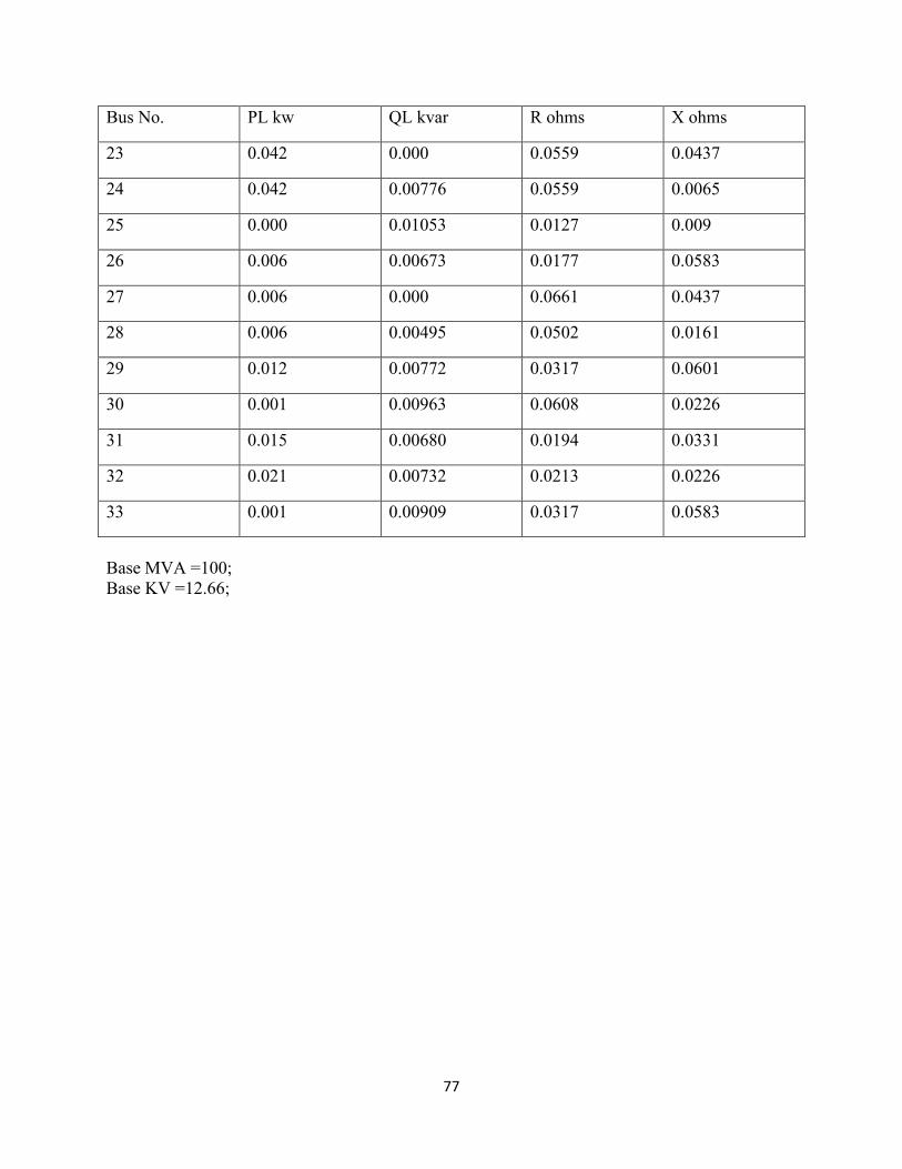
77
Bus No. PL kw QL kvar R ohms X ohms
23 0.042 0.000 0.0559 0.0437
24 0.042 0.00776 0.0559 0.0065
25 0.000 0.01053 0.0127 0.009
26 0.006 0.00673 0.0177 0.0583
27 0.006 0.000 0.0661 0.0437
28 0.006 0.00495 0.0502 0.0161
29 0.012 0.00772 0.0317 0.0601
30 0.001 0.00963 0.0608 0.0226
31 0.015 0.00680 0.0194 0.0331
32 0.021 0.00732 0.0213 0.0226
33 0.001 0.00909 0.0317 0.0583
Base MVA =100;Base KV =12.66;