DRAFT VERSIONAPRIL 13, 2014Preprint typeset using LATEX style emulateapj v. 08/22/09

FARADAY SIGNATURE OF MAGNETIC HELICITY FROM REDUCED DEPOLARIZATION

AXEL BRANDENBURG1,2AND RODION STEPANOV3,4

1Nordita, KTH Royal Institute of Technology and Stockholm University, Roslagstullsbacken 23, 10691 Stockholm, Sweden2Department of Astronomy, AlbaNova University Center, Stockholm University, 10691 Stockholm, Sweden

3Institute of Continuous Media Mechanics, Korolyov str. 1, 614013 Perm, Russia4Perm National Research Polytechnic University, Komsomolskii Av. 29, 614990 Perm, Russia

(Received 2014 January 16, accepted 2014 March 18, Revision: 1.253 )Draft version April 13, 2014

ABSTRACTUsing one-dimensional models, we show that a helical magnetic field with an appropriate sign of helicity

can compensate the Faraday depolarization resulting from the superposition of Faraday-rotated polarizationplanes from a spatially extended source. For radio emissionfrom a helical magnetic field, the polarization asa function of the square of the wavelength becomes asymmetric with respect to zero. Mathematically speak-ing, the resulting emission occurs then either at observable or at unobservable (imaginary) wavelengths. Wedemonstrate that rotation measure (RM) synthesis allows for the reconstruction of the underlying Faraday dis-persion function in the former case, but not in the latter. The presence of positive magnetic helicity can thus bedetected by observing positive RM in highly polarized regions in the sky and negative RM in weakly polarizedregions. Conversely, negative magnetic helicity can be detected by observing negative RM in highly polarizedregions and positive RM in weakly polarized regions. The simultaneous presence of two magnetic constituentswith opposite signs of helicity is shown to possess signatures that can be quantified through polarization peaksat specific wavelengths and the gradient of the phase of the Faraday dispersion function. Similar polarizationpeaks can tentatively also be identified for the bi-helical magnetic fields that are generated self-consistently bya dynamo from helically forced turbulence, even though the magnetic energy spectrum is then continuous. Fi-nally, we discuss the possibility of detecting magnetic fields with helical and non-helical properties in externalgalaxies using the Square Kilometre Array.Subject headings: galaxies: magnetic fields — methods: data analysis — polarization

1. INTRODUCTION

For many decades, polarized radio emission from externalgalaxies has been used to infer the strength and structure oftheir magnetic field. This emission is caused by relativisticelectrons gyrating around magnetic field lines and producingthe polarized synchrotron emission. The plane of polarizationgives an indication about the electric (and thus magnetic) fieldvectors at the source of emission. The line-of-sight compo-nent of the field can be inferred through the Faraday effect thatleads to a wavelength-dependent rotation of the plane of po-larization. The resulting change of the angle of the polariza-tion plane over a certain wavenumber interval gives the rota-tion measure (RM), whose variation across different positionswithin external galaxies gives an idea about the global struc-ture of the magnetic fields of these galaxies (Sofue et al. 1986;Beck et al. 1996, 2005; Fletcher 2010; Beck & Wielebinski2013).

In practice, an observer will always see a superposition ofdifferent polarization planes from different depths, which canlead to a reduction in the degree of polarization. Firstly, theorientation of the magnetic field changes, causing differentpolarization planes at different positions. Secondly, Faradayrotation causes the plane of polarization to rotate. The de-crease in polarized emission resulting from this superpositionis referred to as Faraday depolarization. This was regardedasa problem that can be alleviated partially by restricting one-self to observations at shorter wavelengths (Soida et al. 2011).This situation has changed with the advent of new genera-tions of radio telescopes that can measure polarized emissionover a broad and continuous range of wavelengths. This al-lows one to apply the method of Burn (1966) that utilizes the

wavelength-dependent depolarization to determine the distri-bution of radio sources with respect to Faraday depth (Brent-jens & de Bruyn 2005; Heald et al. 2009; Gießubel et al. 2013;Frick et al. 2011). However, the interpretation of distributedmagnetic fields still remains a challenge (Beck et al. 2012;Bell & Enßlin 2012).

Of particular interest to the present study is the possibil-ity of detecting helicity of the magnetic field. The helicityof the magnetic field reflects the linkage of the magneticfield (Moffatt 1978). In the context of the large-scale mag-netic field in galaxies, one can think of the linkage betweenthe poloidal and toroidal magnetic field components. Three-dimensional visualizations of these two components together,such as Fig. 5 of Donner & Brandenburg (1990), show thatthe magnetic field lines describe a spiralling pattern. An-other manifestation of a helical field is the rotation of a mag-netic field vector perpendicular to the line of sight. Deter-mining the presence of such swirling magnetic field patternswould be an important step toward understanding the natureof the underlying dynamo process that is needed to achievebetter agreement between observations and theory of astro-physical dynamos. A promising result for probing magnetichelicity in the interstellar medium has been obtained by Vole-gova & Stepanov (2010), who have shown that a helical tur-bulent magnetic field produces a nonzero cross-correlationofRM and the degree of polarization. The sign of the cross-correlation coefficient permits one to define the sign of thetotal magnetic helicity. However, the theoretical backgroundof this approach was not clearly understood. Subsequent at-tempts by Junklewitz & Enßlin (2011) and Oppermann et al.(2011) did not clarify this effect either, because they excluded

2

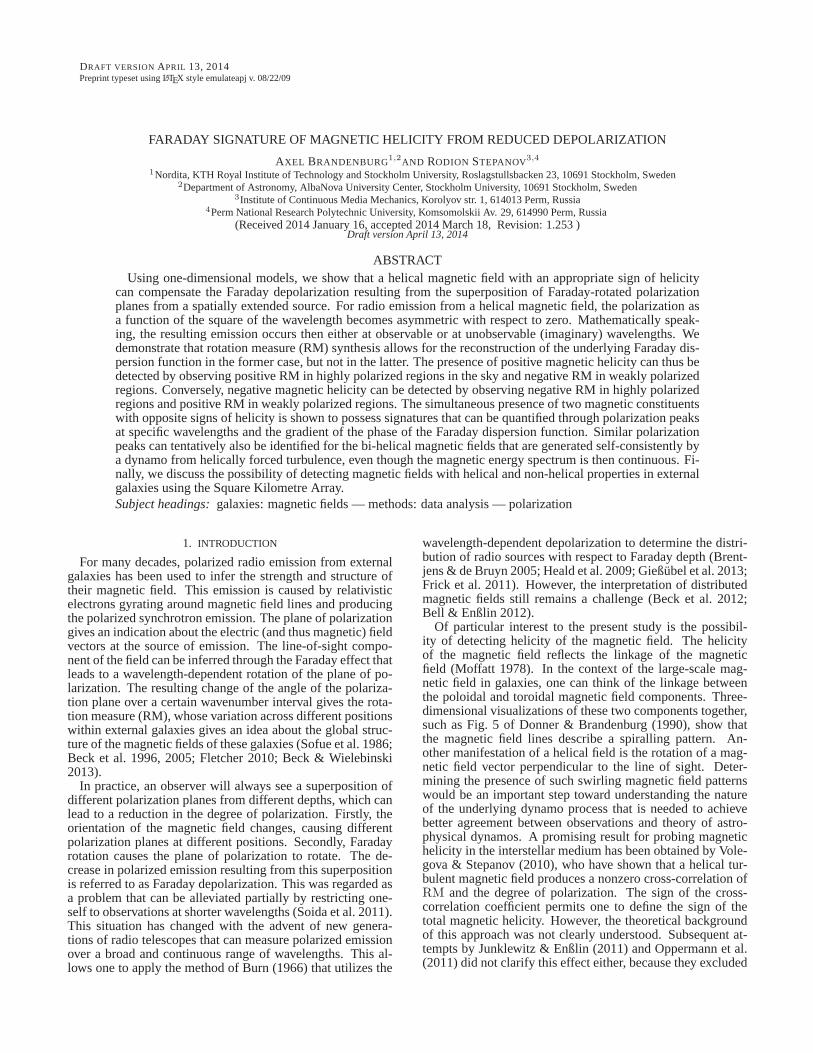
FIG. 1.— Sketch illustrating position of source and observer.

the effect of Faraday depolarization from the beginning. Toexplain the results of Volegova & Stepanov (2010), we stressthe fact that, if the magnetic field is helical, i.e., the mag-netic field lines spiral toward or away from the observer, theresulting Faraday depolarization can be either enhanced orre-duced, depending on the relative signs of magnetic helicityand the line-of-sight component of the magnetic field and thusRM. In a related paper by Horellou & Fletcher (2014), thiseffect was used to study the polarized intensity in selectedwavelength ranges for both signs of helicity. The exploita-tion of this effect, which was first discussed by Sokoloff etal. (1998) as an anomalous depolarization due to a twistedmagnetic field, is an important motivation behind the presentpaper.

While the effect of a helical magnetic field is easily under-stood for simple magnetic spirals, it becomes less obvious inthe case of more complicated fields. We are here particularlyinterested in helical magnetic fields consisting of constituentsthat have large and small length scales with opposite signs ofmagnetic helicity. Such fields are called bi-helical and areofcentral importance in dynamo theory (for a review, see Bran-denburg & Subramanian 2005) and have also been detectedin the solar wind (Brandenburg et al. 2011) and on the solarsurface (Zhang et al. 2014). There is now also some evidencefor helical magnetic fields in the jets emanating from activegalactic nuclei (Reichstein & Gabuzda 2012). We first dis-cuss the observational signatures of singly helical fields andturn then to the case of bi-helical magnetic fields. Next, wediscuss a method referred to as cross-correlation analysisus-ing magnetic field configurations similar to those studied inthe first part of the paper. Those fields are used to mimic theeffects of turbulence consisting of randomly oriented patcheswith singly helical or bi-helical fields oriented randomly inthe sky. Finally, we present preliminary results from more re-alistic magnetic field configurations generated by a turbulentdynamo in the presence of shear. We conclude with a dis-cussion of the possibilities of detecting helical and bi-helicalmagnetic fields in external galaxies using the Square Kilome-tre Array.

2. COMPENSATING DEPOLARIZATION

The synchrotron emission of magnetized interstellar or in-tergalactic media is commonly observed through its total in-tensity,

I(λ2) =

∫ ∞

0

ǫ(z, λ) dz, (1)

and through the StokesQ andU parameters combined into acomplex polarization as

P (λ2) ≡ Q+ iU = p0

∫ ∞

0

ǫ(z, λ)e2i(ψ(z)+φ(z)λ2) dz, (2)

at a given point in the sky. Herep0 is the intrinsic polariza-tion (depending on the energy spectrum of the cosmic rays),ǫ(z, λ) ∝ nc(z)B

σ⊥(z)f(λ) is the polarized emissivity with

σ ≈ 1.9 being an exponent related to the spectral index

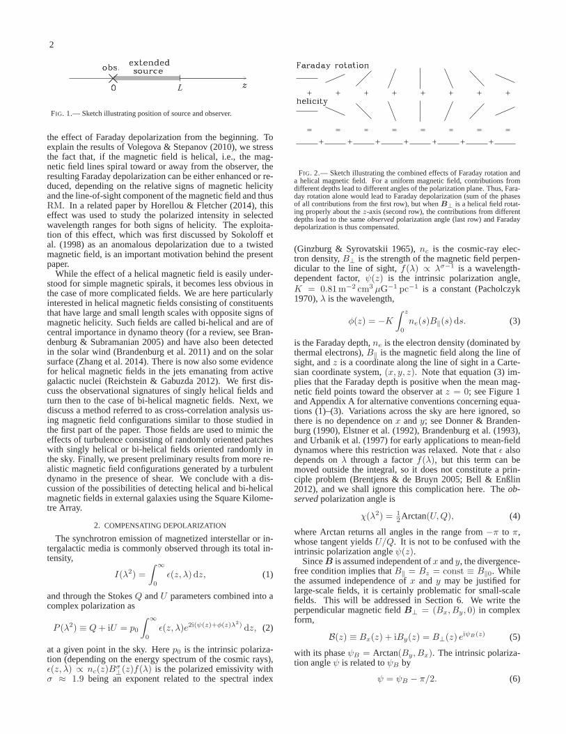
FIG. 2.— Sketch illustrating the combined effects of Faraday rotation anda helical magnetic field. For a uniform magnetic field, contributions fromdifferent depths lead to different angles of the polarization plane. Thus, Fara-day rotation alone would lead to Faraday depolarization (sum of the phasesof all contributions from the first row), but whenB⊥ is a helical field rotat-ing properly about thez-axis (second row), the contributions from differentdepths lead to the sameobserved polarization angle (last row) and Faradaydepolarization is thus compensated.

(Ginzburg & Syrovatskii 1965),nc is the cosmic-ray elec-tron density,B⊥ is the strength of the magnetic field perpen-dicular to the line of sight,f(λ) ∝ λσ−1 is a wavelength-dependent factor,ψ(z) is the intrinsic polarization angle,K = 0.81m−2 cm3 µG−1 pc−1 is a constant (Pacholczyk1970),λ is the wavelength,

φ(z) = −K

∫ z

0

ne(s)B‖(s) ds. (3)

is the Faraday depth,ne is the electron density (dominated bythermal electrons),B‖ is the magnetic field along the line ofsight, andz is a coordinate along the line of sight in a Carte-sian coordinate system,(x, y, z). Note that equation (3) im-plies that the Faraday depth is positive when the mean mag-netic field points toward the observer atz = 0; see Figure 1and Appendix A for alternative conventions concerning equa-tions (1)–(3). Variations across the sky are here ignored, sothere is no dependence onx andy; see Donner & Branden-burg (1990), Elstner et al. (1992), Brandenburg et al. (1993),and Urbanik et al. (1997) for early applications to mean-fielddynamos where this restriction was relaxed. Note thatǫ alsodepends onλ through a factorf(λ), but this term can bemoved outside the integral, so it does not constitute a prin-ciple problem (Brentjens & de Bruyn 2005; Bell & Enßlin2012), and we shall ignore this complication here. Theob-served polarization angle is

χ(λ2) = 12Arctan(U,Q), (4)

where Arctan returns all angles in the range from−π to π,whose tangent yieldsU/Q. It is not to be confused with theintrinsic polarization angleψ(z).

SinceB is assumed independent ofx andy, the divergence-free condition implies thatB‖ = Bz = const ≡ B‖0. Whilethe assumed independence ofx and y may be justified forlarge-scale fields, it is certainly problematic for small-scalefields. This will be addressed in Section 6. We write theperpendicular magnetic fieldB⊥ = (Bx, By, 0) in complexform,

B(z) ≡ Bx(z) + iBy(z) = B⊥(z) eiψB(z) (5)

with its phaseψB = Arctan(By, Bx). The intrinsic polariza-tion angleψ is related toψB by

ψ = ψB − π/2. (6)

3

Here theπ/2 term comes from the fact that the plane of polar-ization is parallel to the electric field and perpendicular to themagnetic field of the radio wave, which, in turn, is parallel tothe ambient fieldB⊥. [Note that this term is sometimes omit-ted; see Waelkens et al. (2009) for such an example. Sokoloffet al. (1998) included it, but dropped the resulting minus signafter their equation (16).] Due to the factor2 in the expo-nent of equation (2), which is a consequence of the definitionof the Stokes parameters being essentially squared quantities,the phase of the magnetic field has aπ ambiguity. This is aserious restriction, because it means that the underlying mag-netic field cannot be determined fully without additional as-sumptions.

We now want to determine a condition on the structure ofthe magnetic field under which the integral in equation (2)gives maximum contribution, that is, for which the Faradaydepolarization is minimal. As was already shown by Sokoloffet al. (1998), this is the case when, for a certain value ofλ, thephase2(ψ(z) + φ(z)λ2) is a constant. For the purpose of thepresent discussion we assume constant values ofB⊥, ne, andnc, denoted byB⊥0, ne0, andnc0, respectively. Therefore,φ(z) = −Kne0B‖0z is linear inz, and so the (half) phaseunder the integral in equation (2) is given by

ψ(z) + φ(z)λ2 = ψ(z)−Kne0B‖0λ2z, (7)

which becomes independent ofz and equal to a constantψ0,giving thus maximum contribution to the integral, when

ψB(z) = ψ0 − kz, (8)

whereψ0 is an arbitrary phase shift and

k = −Kne0B‖0λ2 (9)

is the required wavenumber of the magnetic field. A simi-lar condition was also derived by Arshakian & Beck (2011),without however explicitly making reference to the helicalna-ture of the magnetic field.

Equation (8) implies that we have aunique solution for themagnetic field that gives maximum contribution to the inte-gral in equation (2) by essentially canceling the Faraday de-polarization from theexp(2iφλ2) term, as illustrated in Fig-ure 2. Inserting equation (8) into equation (5) and assumingB⊥ = const, we have

B =(

B⊥0 cos(kz − ψ0),−B⊥0 sin(kz − ψ0), B‖0

)

. (10)

Such a twisted magnetic field withψB(z) ∝ z is a Beltramifield and has been considered by Sokoloff et al. (1998) for thedemonstration of anomalous depolarization.

As motivated above, we are interested in the magnetic he-licity of the field. It is defined as〈A · B〉, where angu-lar brackets denote volume averaging andA is the mag-netic vector potential withB = ∇ × A and componentsA = (Bx/k,By/k + xB‖0, 0). Here the linearly varyingcomponentxB‖0 is needed to give the constantB‖ = B‖0,but this contribution averages out in the calculation of themagnetic helicity,

〈A ·B〉 = k−1B2⊥0. (11)

Another quantity of interest, which is based on the currentdensityJ = ∇ × B/µ0 with µ0 being the vacuum perme-ability, is the current helicity,〈J · B〉 = kB2

⊥0/µ0. In thepresent example, it has the same sign as〈A·B〉 and is positive(negative) for positive (negative) values ofk. Note also that

ψB decreases (increases) withz when the magnetic helicity ispositive (negative). Somewhat surprisingly, this impliesthatthe tips of the magnetic field vectors describe a left-handed(right-handed) spiral when magnetic helicity is positive (neg-ative).

For agiven magnetic field, that is, prescribedk andB‖0,|P (λ2)| as a function ofλ becomes maximal if equation (9)holds, that isλ2 = −k/Kne0B‖0. Obviously, onlyλ2 >0 is observable, so only negative (positive) helicities can bedetected via the observation of a maximum of|P (λ2)| if B‖0

is positive (negative), i.e., the field points away from (toward)the observer.

To give an example for typical values of the radio wave-length expected from magnetic fields in the interstellarmedium and in external galaxies, let us takek = 2π/ kpc forthe wavenumber of a field of one kpc scale,ne0 = 0.03 cm−3

(Taylor & Cordes 1993), andB‖0 = 3µG, then|P (λ2)| peaksat λ ≈ 30 cm. To probe fields with larger (smaller) lengthscales, one would need shorter (longer) wavelengths of theradio emission.

3. FARADAY DISPERSION FUNCTION

To characterize the observational signature of a helicalmagnetic field, we compute the corresponding complex po-larization as a function ofλ2 using equation (2). For the pur-pose of further analysis the polarization can be expressed as aFourier integral,

P (λ2) =

∫ ∞

−∞

F (φ) e2iφλ2

dφ, (12)

whereF (φ) = f(φ) e2iψ(φ) (13)

is called the Faraday dispersion function (Burn 1966) withf(φ) = |F (φ)|. Provided that equation (3) defines a strictlymonotonous functionφ(z), we havedφ/dz 6= 0 and canchange variables fromz to φ in equation (2), and we write

f(φ) = −p0ǫ(φ)/Kne(φ)B‖(φ), (14)

where the denominator is justdφ/dz resulting from the trans-formation fromz to φ. The factor2 in the exponent of equa-tion (13) results in theπ ambiguity. It is therefore useful tocharacterize signatures of helical magnetic fields directly interms ofF (φ). This is particularly important, because thereis, at least in principle, the chance to reconstructF (φ) fromP (λ2) using Fourier transformation with respect to the conju-gate variable2λ2 (Burn 1966). Given the lack of any informa-tion aboutP (λ2) for λ2 < 0 we define the synthesized Fara-day dispersion function (Burn 1966; Brentjens & de Bruyn2005),

Fsyn(φ) =1

2π

∫ ∞

0

P (λ2) e−2iφλ2

d(2λ2), (15)

which is supposed to be a reasonable approximation of theactualF (φ), which would be obtained if the integral in equa-tion (15) were from−∞ to∞.

We now consider a concrete example using equation (10)with k = k1 to construct a magnetic field in a slab of thicknessL with 0 ≤ z < L. In the following, we take|k1| = 2π/L,i.e., we have within the slab just two nodes in each of the twocomponents ofB⊥. Outside this range, we assumeB⊥ = 0,but we keepB‖ = B‖0 everywhere. The Faraday depth,

4

φ = −Kne0B‖0z, is a uniformly varying coordinate andR ≡ φ(L) = −Kne0B‖0L is the equivalent intrinsic Faradayrotation measure or simply the Faraday thickness of the slab.Thenǫ(φ) 6= 0 is the range0 ≤ φ/R ≤ 1. For normalizationpurposes we introduce here the wavelengthλ1. It is given by

λ21 = −k1/Kne0B‖0 (16)

and determines the peak of the modulus of the resulting com-plex polarization,

P (λ2) = p0I P(

R(λ2 − λ21))

, (17)

whereP (ξ) =

(

1− e2iξ)/

2iξ (18)

is Burn’s non-dimensional depolarization function, indicatedby a hat. It applies in the absence of magnetic helicity to a uni-form slab of Faraday thicknessR. Note that in our normaliza-tion, P (0) = −1, where the minus sign is a consequence oftheπ/2 term in equation (6). Note also thatd arg(P )/dξ = 1,in spite of the factor2 in the exponential function in equa-tion (18).

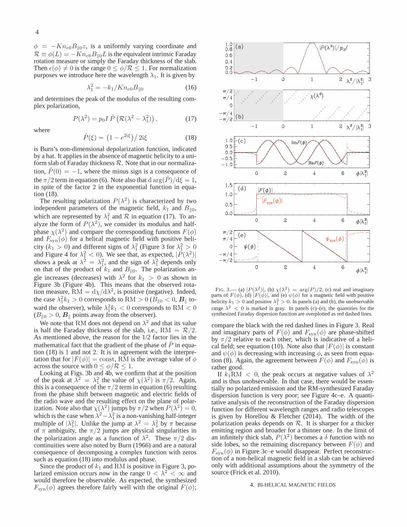
The resulting polarizationP (λ2) is characterized by twoindependent parameters of the magnetic field,k1 andB‖0,which are represented byλ21 andR in equation (17). To an-alyze the form ofP (λ2), we consider its modulus and half-phaseχ(λ2) and compare the corresponding functionsF (φ)andFsyn(φ) for a helical magnetic field with positive heli-city (k1 > 0) and different signs ofλ21 (Figure 3 forλ21 > 0and Figure 4 forλ21 < 0). We see that, as expected,|P (λ2)|shows a peak atλ2 = λ21, and the sign ofλ21 depends onlyon that of the product ofk1 andB‖0. The polarization an-gle increases (decreases) withλ2 for k1 > 0 as shown inFigure 3b (Figure 4b). This means that the observed rota-tion measure,RM = dχ/dλ2, is positive (negative). Indeed,the caseλ21k1 > 0 corresponds toRM > 0 (B‖0 < 0, B‖ to-ward the observer), whileλ21k1 < 0 corresponds toRM < 0(B‖0 > 0, B‖ points away from the observer).

We note thatRM does not depend onλ2 and that its valueis half the Faraday thickness of the slab, i.e.,RM = R/2.As mentioned above, the reason for the 1/2 factor lies in themathematical fact that the gradient of the phase ofP in equa-tion (18) is1 and not2. It is in agreement with the interpre-tation that for|F (φ)| = const, RM is the average value ofφacross the source with0 ≤ φ/R ≤ 1.

Looking at Figs. 3b and 4b, we confirm that at the positionof the peak atλ2 = λ21 the value ofχ(λ2) is π/2. Again,this is a consequence of theπ/2 term in equation (6) resultingfrom the phase shift between magnetic and electric fields ofthe radio wave and the resulting effect on the plane of polar-ization. Note also thatχ(λ2) jumps byπ/2 whenP (λ2) = 0,which is the case whenλ2−λ21 is a non-vanishing half-integermultiple of |λ21|. Unlike the jump atλ2 = λ21 by π becauseof π ambiguity, theπ/2 jumps are physical singularities inthe polarization angle as a function ofλ2. Theseπ/2 dis-continuities were also noted by Burn (1966) and are a naturalconsequence of decomposing a complex function with zerossuch as equation (18) into modulus and phase.

Since the product ofk1 andRM is positive in Figure 3, po-larized emission occurs now in the range0 < λ2 < ∞ andwould therefore be observable. As expected, the synthesizedFsyn(φ) agrees therefore fairly well with the originalF (φ);

FIG. 3.— (a) |P (λ2)|, (b) χ(λ2) = arg(P )/2, (c) real and imaginaryparts ofF (φ), (d) |F (φ)|, and (e)ψ(φ) for a magnetic field with positivehelicity k1 > 0 and positiveλ2

1> 0. In panels (a) and (b), the unobservable

rangeλ2 < 0 is marked in gray. In panels (c)–(e), the quantities for thesynthesized Faraday dispersion function are overplotted as red dashed lines.

compare the black with the red dashed lines in Figure 3. Realand imaginary parts ofF (φ) andFsyn(φ) are phase-shiftedby π/2 relative to each other, which is indicative of a heli-cal field; see equation (10). Note also that|F (φ)| is constantandψ(φ) is decreasing with increasingφ, as seen from equa-tion (8). Again, the agreement betweenF (φ) andFsyn(φ) israther good.

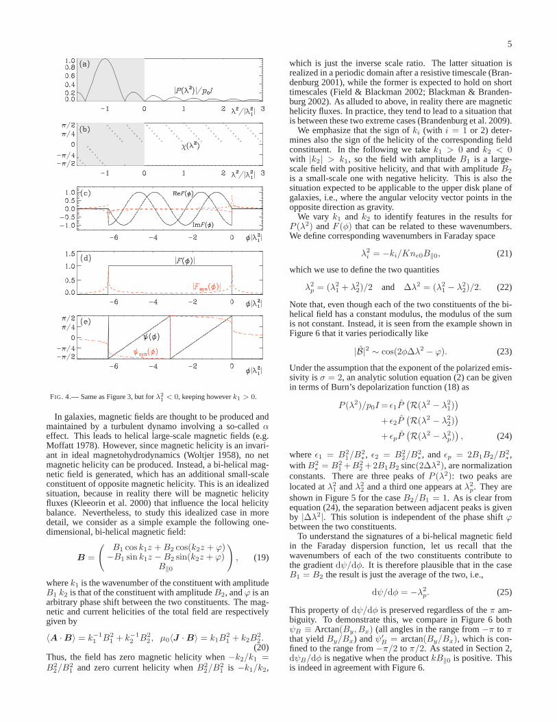
If k1RM < 0, the peak occurs at negative values ofλ2

and is thus unobservable. In that case, there would be essen-tially no polarized emission and the RM-synthesized Faradaydispersion function is very poor; see Figure 4c–e. A quanti-tative analysis of the reconstruction of the Faraday dispersionfunction for different wavelength ranges and radio telescopesis given by Horellou & Fletcher (2014). The width of thepolarization peaks depends onR. It is sharper for a thickeremitting region and broader for a thinner one. In the limit ofan infinitely thick slab,P (λ2) becomes aδ function with noside lobes, so the remaining discrepancy betweenF (φ) andFsyn(φ) in Figure 3c–e would disappear. Perfect reconstruc-tion of a non-helical magnetic field in a slab can be achievedonly with additional assumptions about the symmetry of thesource (Frick et al. 2010).

4. BI-HELICAL MAGNETIC FIELDS

5

FIG. 4.— Same as Figure 3, but forλ21< 0, keeping howeverk1 > 0.

In galaxies, magnetic fields are thought to be produced andmaintained by a turbulent dynamo involving a so-calledαeffect. This leads to helical large-scale magnetic fields (e.g.Moffatt 1978). However, since magnetic helicity is an invari-ant in ideal magnetohydrodynamics (Woltjer 1958), no netmagnetic helicity can be produced. Instead, a bi-helical mag-netic field is generated, which has an additional small-scaleconstituent of opposite magnetic helicity. This is an idealizedsituation, because in reality there will be magnetic helicityfluxes (Kleeorin et al. 2000) that influence the local helicitybalance. Nevertheless, to study this idealized case in moredetail, we consider as a simple example the following one-dimensional, bi-helical magnetic field:

B =

(

B1 cos k1z +B2 cos(k2z + ϕ)−B1 sin k1z −B2 sin(k2z + ϕ)

B‖0

)

, (19)

wherek1 is the wavenumber of the constituent with amplitudeB1 k2 is that of the constituent with amplitudeB2, andϕ is anarbitrary phase shift between the two constituents. The mag-netic and current helicities of the total field are respectivelygiven by

〈A ·B〉 = k−11 B2

1 + k−12 B2

2 , µ0〈J ·B〉 = k1B21 + k2B

22 .

(20)Thus, the field has zero magnetic helicity when−k2/k1 =B2

2/B21 and zero current helicity whenB2

2/B21 is −k1/k2,

which is just the inverse scale ratio. The latter situation isrealized in a periodic domain after a resistive timescale (Bran-denburg 2001), while the former is expected to hold on shorttimescales (Field & Blackman 2002; Blackman & Branden-burg 2002). As alluded to above, in reality there are magnetichelicity fluxes. In practice, they tend to lead to a situationthatis between these two extreme cases (Brandenburg et al. 2009).

We emphasize that the sign ofki (with i = 1 or 2) deter-mines also the sign of the helicity of the corresponding fieldconstituent. In the following we takek1 > 0 andk2 < 0with |k2| > k1, so the field with amplitudeB1 is a large-scale field with positive helicity, and that with amplitudeB2

is a small-scale one with negative helicity. This is also thesituation expected to be applicable to the upper disk plane ofgalaxies, i.e., where the angular velocity vector points intheopposite direction as gravity.

We vary k1 and k2 to identify features in the results forP (λ2) andF (φ) that can be related to these wavenumbers.We define corresponding wavenumbers in Faraday space

λ2i = −ki/Kne0B‖0, (21)

which we use to define the two quantities

λ2p = (λ21 + λ22)/2 and ∆λ2 = (λ21 − λ22)/2. (22)

Note that, even though each of the two constituents of the bi-helical field has a constant modulus, the modulus of the sumis not constant. Instead, it is seen from the example shown inFigure 6 that it varies periodically like

|B|2 ∼ cos(2φ∆λ2 − ϕ). (23)

Under the assumption that the exponent of the polarized emis-sivity is σ = 2, an analytic solution equation (2) can be givenin terms of Burn’s depolarization function (18) as

P (λ2)/p0I= ǫ1P(

R(λ2 − λ21))

+ ǫ2P(

R(λ2 − λ22))

+ ǫpP(

R(λ2 − λ2p))

, (24)

whereǫ1 = B21/B

2∗ , ǫ2 = B2

2/B2∗ , andǫp = 2B1B2/B

2∗ ,

withB2∗ = B2

1 +B22 +2B1B2 sinc(2∆λ2), are normalization

constants. There are three peaks ofP (λ2): two peaks arelocated atλ21 andλ22 and a third one appears atλ2p. They areshown in Figure 5 for the caseB2/B1 = 1. As is clear fromequation (24), the separation between adjacent peaks is givenby |∆λ2|. This solution is independent of the phase shiftϕbetween the two constituents.

To understand the signatures of a bi-helical magnetic fieldin the Faraday dispersion function, let us recall that thewavenumbers of each of the two constituents contribute tothe gradientdψ/dφ. It is therefore plausible that in the caseB1 = B2 the result is just the average of the two, i.e.,

dψ/dφ = −λ2p. (25)

This property ofdψ/dφ is preserved regardless of theπ am-biguity. To demonstrate this, we compare in Figure 6 bothψB ≡ Arctan(By, Bx) (all angles in the range from−π to πthat yieldBy/Bx) andψ′

B = arctan(By/Bx), which is con-fined to the range from−π/2 to π/2. As stated in Section 2,dψB/dφ is negative when the productkB‖0 is positive. Thisis indeed in agreement with Figure 6.

6

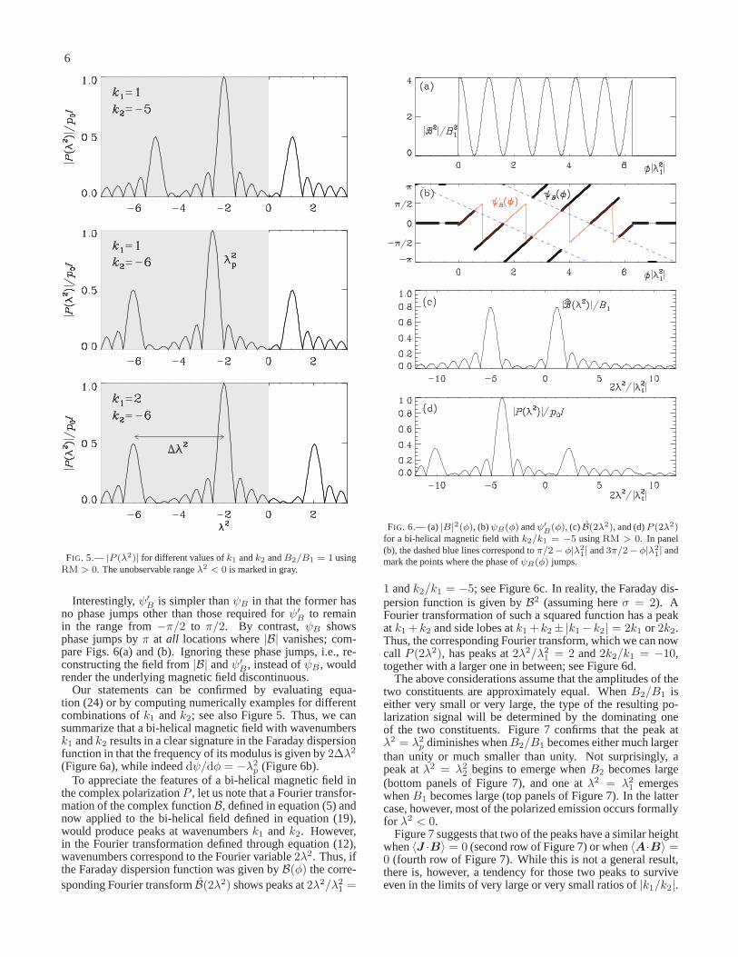
FIG. 5.— |P (λ2)| for different values ofk1 andk2 andB2/B1 = 1 usingRM > 0. The unobservable rangeλ2 < 0 is marked in gray.

Interestingly,ψ′B is simpler thanψB in that the former has

no phase jumps other than those required forψ′B to remain

in the range from−π/2 to π/2. By contrast,ψB showsphase jumps byπ at all locations where|B| vanishes; com-pare Figs. 6(a) and (b). Ignoring these phase jumps, i.e., re-constructing the field from|B| andψ′

B , instead ofψB , wouldrender the underlying magnetic field discontinuous.

Our statements can be confirmed by evaluating equa-tion (24) or by computing numerically examples for differentcombinations ofk1 andk2; see also Figure 5. Thus, we cansummarize that a bi-helical magnetic field with wavenumbersk1 andk2 results in a clear signature in the Faraday dispersionfunction in that the frequency of its modulus is given by2∆λ2

(Figure 6a), while indeeddψ/dφ = −λ2p (Figure 6b).To appreciate the features of a bi-helical magnetic field in

the complex polarizationP , let us note that a Fourier transfor-mation of the complex functionB, defined in equation (5) andnow applied to the bi-helical field defined in equation (19),would produce peaks at wavenumbersk1 andk2. However,in the Fourier transformation defined through equation (12),wavenumbers correspond to the Fourier variable2λ2. Thus, ifthe Faraday dispersion function was given byB(φ) the corre-sponding Fourier transformB(2λ2) shows peaks at2λ2/λ21 =

FIG. 6.— (a)|B|2(φ), (b)ψB(φ) andψ′B(φ), (c) B(2λ2), and (d)P (2λ2)

for a bi-helical magnetic field withk2/k1 = −5 usingRM > 0. In panel(b), the dashed blue lines correspond toπ/2− φ|λ2

1| and3π/2− φ|λ2

1| and

mark the points where the phase ofψB(φ) jumps.

1 andk2/k1 = −5; see Figure 6c. In reality, the Faraday dis-persion function is given byB2 (assuming hereσ = 2). AFourier transformation of such a squared function has a peakatk1+k2 and side lobes atk1+k2±|k1−k2| = 2k1 or 2k2.Thus, the corresponding Fourier transform, which we can nowcall P (2λ2), has peaks at2λ2/λ21 = 2 and2k2/k1 = −10,together with a larger one in between; see Figure 6d.

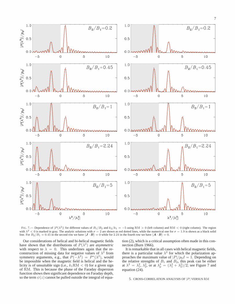
The above considerations assume that the amplitudes of thetwo constituents are approximately equal. WhenB2/B1 iseither very small or very large, the type of the resulting po-larization signal will be determined by the dominating oneof the two constituents. Figure 7 confirms that the peak atλ2 = λ2p diminishes whenB2/B1 becomes either much largerthan unity or much smaller than unity. Not surprisingly, apeak atλ2 = λ22 begins to emerge whenB2 becomes large(bottom panels of Figure 7), and one atλ2 = λ21 emergeswhenB1 becomes large (top panels of Figure 7). In the lattercase, however, most of the polarized emission occurs formallyfor λ2 < 0.

Figure 7 suggests that two of the peaks have a similar heightwhen〈J ·B〉 = 0 (second row of Figure 7) or when〈A·B〉 =0 (fourth row of Figure 7). While this is not a general result,there is, however, a tendency for those two peaks to surviveeven in the limits of very large or very small ratios of|k1/k2|.

7

FIG. 7.— Dependence of|P (λ2)| for different values ofB1/B2 andk2/k1 = −5 usingRM > 0 (left column) andRM < 0 (right column). The regionwith λ2 < 0 is marked in gray. The analytic solutions withσ = 2 are shown as red dotted lines, while the numerical one forσ = 1.9 is shown as a black solidline. ForB2/B1 = 0.45 in the second row we have〈J ·B〉 = 0 while for 2.24 in the fourth row we have〈A ·B〉 = 0.

Our considerations of helical and bi-helical magnetic fieldshave shown that the distributions ofP (λ2) are asymmetricwith respect toλ = 0. This underlines again that the re-construction of missing data for negative values ofλ2 fromsymmetry arguments, e.g., thatP (−λ2) = P ∗(λ2), wouldbe impossible when the magnetic field is helical and the he-licity is of unsuitable sign (i.e.,k1RM < 0) for a given signof RM. This is because the phase of the Faraday dispersionfunction shows then significant dependence on Faraday depth,so the termψ(z) cannot be pulled outside the integral of equa-

tion (2), which is a critical assumption often made in this con-nection (Burn 1966).

It is remarkable that in all cases with helical magnetic fields,there is a particular valueλ2 for which the polarization ap-proaches the maximum value of|P |/p0I = 1. Depending onthe relative strengths ofB1 andB2, this peak can be eitherat λ2 = λ21, λ22, or atλ2p = (λ21 + λ22)/2; see Figure 7 andequation (24).

5. CROSS-CORRELATION ANALYSIS OF|P | VERSUSRM

8

Our present investigations have implications that help un-derstand earlier work in the field. Recent surveys of polarizedemission in the interstellar medium have provided continu-ous distributions ofQ andU on the sky for certain ranges ofwavelengths. Due to finite beam size, only a small number ofindependent lines of sight are available for analysis. Probingmagnetic helicity with a cross-correlation analysis betweenRM and the polarization degreeP ≡ |P |/p0I had been sug-gested by Volegova & Stepanov (2010) using simulated data.While the numerical demonstration of the method was con-vincing, no theoretical proof or explanation had been avail-able yet.

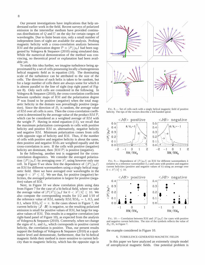
To study this idea further, we imagine turbulence being ap-proximated by a set of cells possessing locally a homogeneoushelical magnetic field as in equation (10). The dominatingscale of the turbulence can be attributed to the size of thecells. The direction of each helix is taken to be random, butfor a large number of cells there are always some for which itis almost parallel to the line of sight (top right panel of Fig-ure 8). Only such cells are considered in the following. InVolegova & Stepanov (2010), the cross-correlation coefficientbetween synthetic maps ofRM and the polarization degreeP was found to be positive (negative) when the total mag-netic helicity in the domain was prevailingly positive (nega-tive). Since the direction ofB‖ is random, the average valueof RM over all cells is zero. Then the cross-correlation coeffi-cient is determined by the average value of the productRMP,which can be considered as a weighted average ofRM withthe weightP. Having in mind equation (11), we recall thatthe maximum polarization corresponds to cells with positivehelicity and positiveRM or, alternatively, negative helicityand negativeRM. Minimum polarization comes from cellswith opposite sign of helicity andRM. Thus, if the numberof cells with positive and negative helicity is about the same,then positive and negativeRMs are weighted equally and thecross-correlation is zero. If the cells with positive (negative)helicity are dominant, then〈RMP〉 is positive (negative).

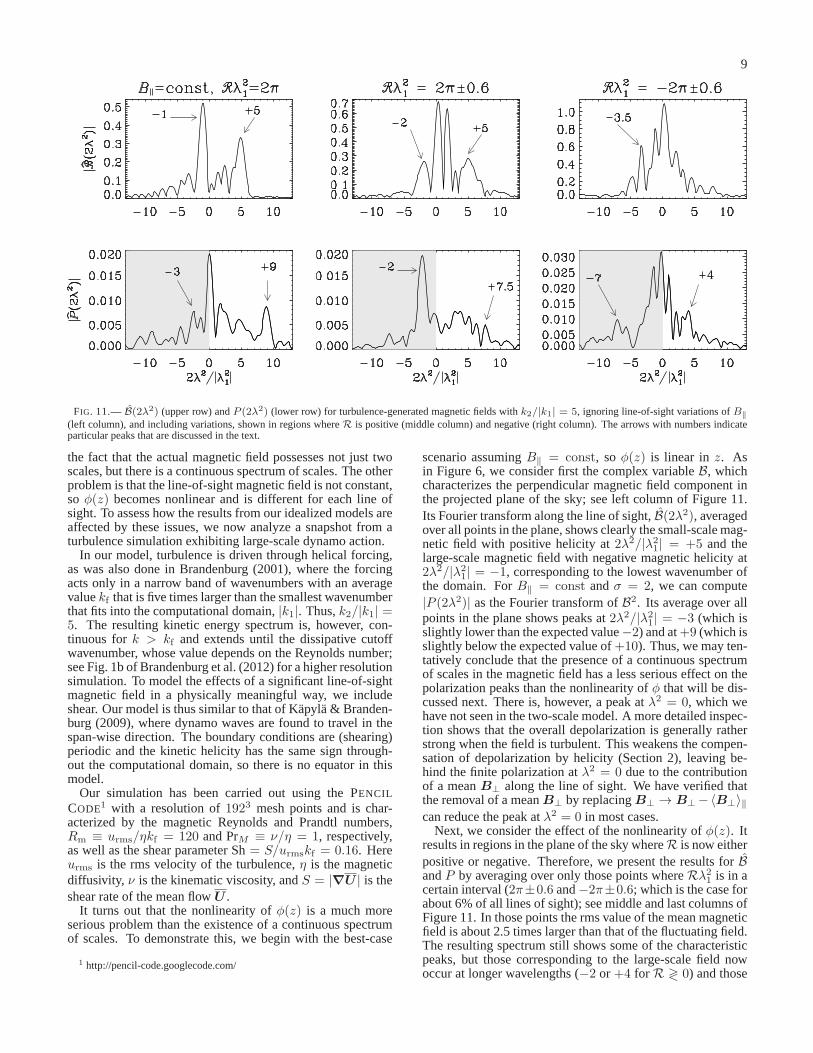
In the following, another test is suggested for the cross-correlation diagnostics. We consider the averaged polariza-tion 〈|P |/p0I〉 by averaging overλ2, using however only onecell. In Figure 9 we show first the dependence of〈|P |/p0I〉onRM for different wavenumbers using a singly helical mag-netic field. Here we have averaged over wavelengths in therange0 < λ2 ≤ λ21. We see that, for positive (negative) he-licities, the averaged polarization is largest for positive (nega-tive) values ofRM.

Next, in Figure 10 we show correlation plots using datafrom Figure 7 for the case of a bi-helical field, where we takethe average value of|P (λ2)|/p0I for 0 < λ2/λ21 ≤ 10. Wealso compute the corresponding results for 1/2 and 1/10 ofthe reference value ofRM, namelyRM/RM0 = 1, 0.5, and0.1, whereRM0λ

21 = π. In the cases shown in Figure 7, the

current helicity〈J ·B〉 is negative, so the resulting polarizedemission is small for positive values ofRM, but large for neg-ative values ofRM. This results in a negative correlation (seeright-hand panel of Figure 10), as expected from the analysisof Volegova & Stepanov (2010). Conversely, when we changethe signs ofk1 andk2, which corresponds to positive currenthelicity, the correlation is positive. Thus, our present resultssupport the findings of Volegova & Stepanov (2010) at a qual-itative level and demonstrate, furthermore, that for bi-helicalmagnetic fields their method is more sensitive to current heli-city than to magnetic helicity, which has the opposite sign in

FIG. 8.— Set of cells each with a singly helical magnetic field of positivehelicity. The tips of the vectors describe a left-handed spiral.

FIG. 9.— Dependence of〈P/p0I〉 on RM for different wavenumbersk(relative to a reference wavenumberk1) and cases with positive and negativecurrent helicities (positive and negative values ofk) using an average over0 < λ2/λ2

1≤ 10.

FIG. 10.— Correlation betweenRM and〈P/p0I〉 for cases with positiveand negative current helicities. The size of the symbols reflects the value ofB2/B1 in Figure 7.

the example considered in Figure 10.

6. TURBULENCE-GENERATED MAGNETIC FIELDS

In this paper we have analyzed an extremely simple modelof astrophysical magnetic fields. One potential problem is

9

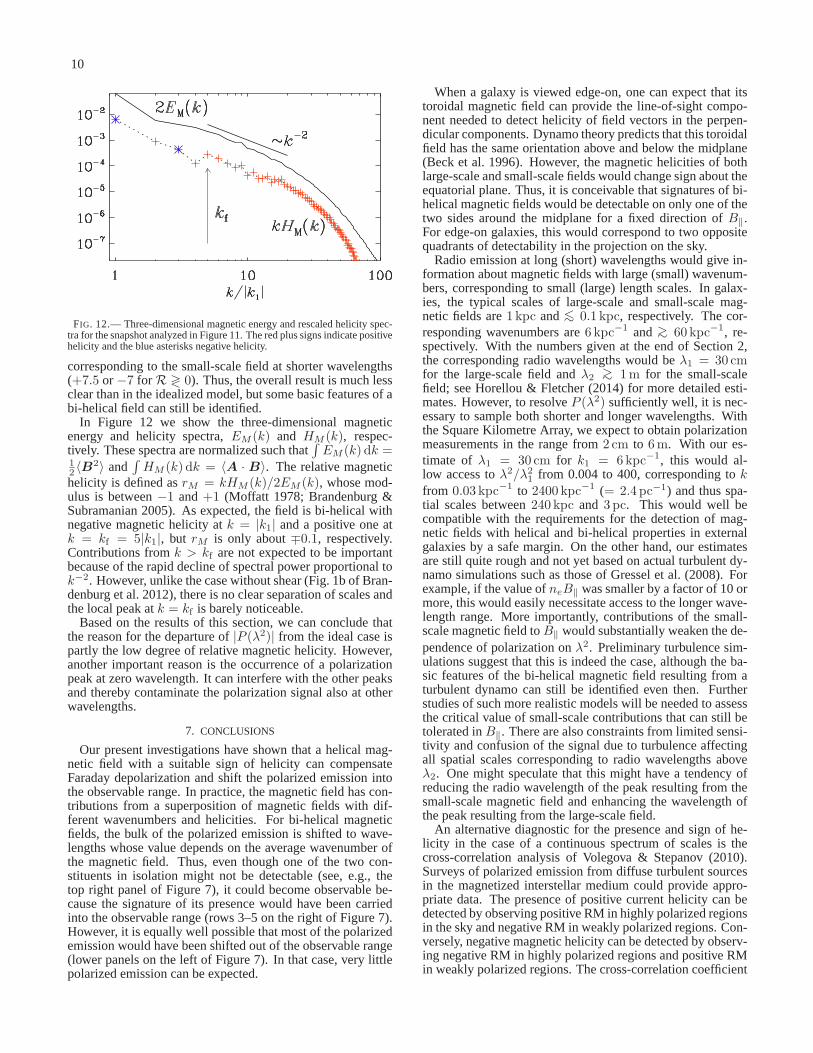
FIG. 11.— B(2λ2) (upper row) andP (2λ2) (lower row) for turbulence-generated magnetic fields withk2/|k1| = 5, ignoring line-of-sight variations ofB‖

(left column), and including variations, shown in regions whereR is positive (middle column) and negative (right column). The arrows with numbers indicateparticular peaks that are discussed in the text.

the fact that the actual magnetic field possesses not just twoscales, but there is a continuous spectrum of scales. The otherproblem is that the line-of-sight magnetic field is not constant,so φ(z) becomes nonlinear and is different for each line ofsight. To assess how the results from our idealized models areaffected by these issues, we now analyze a snapshot from aturbulence simulation exhibiting large-scale dynamo action.

In our model, turbulence is driven through helical forcing,as was also done in Brandenburg (2001), where the forcingacts only in a narrow band of wavenumbers with an averagevaluekf that is five times larger than the smallest wavenumberthat fits into the computational domain,|k1|. Thus,k2/|k1| =5. The resulting kinetic energy spectrum is, however, con-tinuous fork > kf and extends until the dissipative cutoffwavenumber, whose value depends on the Reynolds number;see Fig. 1b of Brandenburg et al. (2012) for a higher resolutionsimulation. To model the effects of a significant line-of-sightmagnetic field in a physically meaningful way, we includeshear. Our model is thus similar to that of Kapyla & Branden-burg (2009), where dynamo waves are found to travel in thespan-wise direction. The boundary conditions are (shearing)periodic and the kinetic helicity has the same sign through-out the computational domain, so there is no equator in thismodel.

Our simulation has been carried out using the PENCIL

CODE1 with a resolution of1923 mesh points and is char-acterized by the magnetic Reynolds and Prandtl numbers,Rm ≡ urms/ηkf = 120 and PrM ≡ ν/η = 1, respectively,as well as the shear parameter Sh= S/urmskf = 0.16. Hereurms is the rms velocity of the turbulence,η is the magneticdiffusivity, ν is the kinematic viscosity, andS = |∇U | is theshear rate of the mean flowU .

It turns out that the nonlinearity ofφ(z) is a much moreserious problem than the existence of a continuous spectrumof scales. To demonstrate this, we begin with the best-case

1 http://pencil-code.googlecode.com/

scenario assumingB‖ = const, soφ(z) is linear inz. Asin Figure 6, we consider first the complex variableB, whichcharacterizes the perpendicular magnetic field component inthe projected plane of the sky; see left column of Figure 11.Its Fourier transform along the line of sight,B(2λ2), averagedover all points in the plane, shows clearly the small-scale mag-netic field with positive helicity at2λ2/|λ21| = +5 and thelarge-scale magnetic field with negative magnetic helicityat2λ2/|λ21| = −1, corresponding to the lowest wavenumber ofthe domain. ForB‖ = const andσ = 2, we can compute|P (2λ2)| as the Fourier transform ofB2. Its average over allpoints in the plane shows peaks at2λ2/|λ21| = −3 (which isslightly lower than the expected value−2) and at+9 (which isslightly below the expected value of+10). Thus, we may ten-tatively conclude that the presence of a continuous spectrumof scales in the magnetic field has a less serious effect on thepolarization peaks than the nonlinearity ofφ that will be dis-cussed next. There is, however, a peak atλ2 = 0, which wehave not seen in the two-scale model. A more detailed inspec-tion shows that the overall depolarization is generally ratherstrong when the field is turbulent. This weakens the compen-sation of depolarization by helicity (Section 2), leaving be-hind the finite polarization atλ2 = 0 due to the contributionof a meanB⊥ along the line of sight. We have verified thatthe removal of a meanB⊥ by replacingB⊥ → B⊥−〈B⊥〉‖can reduce the peak atλ2 = 0 in most cases.

Next, we consider the effect of the nonlinearity ofφ(z). Itresults in regions in the plane of the sky whereR is now eitherpositive or negative. Therefore, we present the results forBandP by averaging over only those points whereRλ21 is in acertain interval (2π±0.6 and−2π±0.6; which is the case forabout 6% of all lines of sight); see middle and last columns ofFigure 11. In those points the rms value of the mean magneticfield is about 2.5 times larger than that of the fluctuating field.The resulting spectrum still shows some of the characteristicpeaks, but those corresponding to the large-scale field nowoccur at longer wavelengths (−2 or +4 for R ≷ 0) and those

10

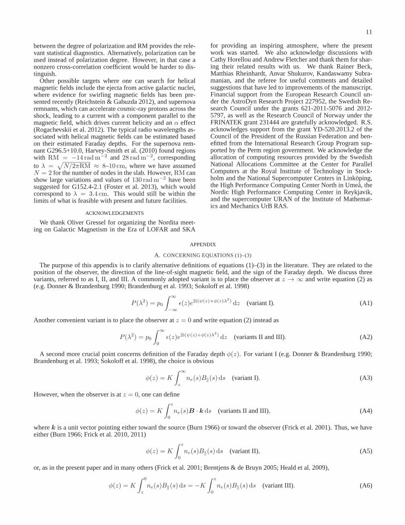
FIG. 12.— Three-dimensional magnetic energy and rescaled helicity spec-tra for the snapshot analyzed in Figure 11. The red plus signsindicate positivehelicity and the blue asterisks negative helicity.

corresponding to the small-scale field at shorter wavelengths(+7.5 or−7 for R ≷ 0). Thus, the overall result is much lessclear than in the idealized model, but some basic features ofabi-helical field can still be identified.

In Figure 12 we show the three-dimensional magneticenergy and helicity spectra,EM (k) and HM (k), respec-tively. These spectra are normalized such that

∫

EM (k) dk =12 〈B

2〉 and∫

HM (k) dk = 〈A · B〉. The relative magnetichelicity is defined asrM = kHM (k)/2EM (k), whose mod-ulus is between−1 and+1 (Moffatt 1978; Brandenburg &Subramanian 2005). As expected, the field is bi-helical withnegative magnetic helicity atk = |k1| and a positive one atk = kf = 5|k1|, but rM is only about∓0.1, respectively.Contributions fromk > kf are not expected to be importantbecause of the rapid decline of spectral power proportionaltok−2. However, unlike the case without shear (Fig. 1b of Bran-denburg et al. 2012), there is no clear separation of scales andthe local peak atk = kf is barely noticeable.

Based on the results of this section, we can conclude thatthe reason for the departure of|P (λ2)| from the ideal case ispartly the low degree of relative magnetic helicity. However,another important reason is the occurrence of a polarizationpeak at zero wavelength. It can interfere with the other peaksand thereby contaminate the polarization signal also at otherwavelengths.

7. CONCLUSIONS

Our present investigations have shown that a helical mag-netic field with a suitable sign of helicity can compensateFaraday depolarization and shift the polarized emission intothe observable range. In practice, the magnetic field has con-tributions from a superposition of magnetic fields with dif-ferent wavenumbers and helicities. For bi-helical magneticfields, the bulk of the polarized emission is shifted to wave-lengths whose value depends on the average wavenumber ofthe magnetic field. Thus, even though one of the two con-stituents in isolation might not be detectable (see, e.g., thetop right panel of Figure 7), it could become observable be-cause the signature of its presence would have been carriedinto the observable range (rows 3–5 on the right of Figure 7).However, it is equally well possible that most of the polarizedemission would have been shifted out of the observable range(lower panels on the left of Figure 7). In that case, very littlepolarized emission can be expected.

When a galaxy is viewed edge-on, one can expect that itstoroidal magnetic field can provide the line-of-sight compo-nent needed to detect helicity of field vectors in the perpen-dicular components. Dynamo theory predicts that this toroidalfield has the same orientation above and below the midplane(Beck et al. 1996). However, the magnetic helicities of bothlarge-scale and small-scale fields would change sign about theequatorial plane. Thus, it is conceivable that signatures of bi-helical magnetic fields would be detectable on only one of thetwo sides around the midplane for a fixed direction ofB‖.For edge-on galaxies, this would correspond to two oppositequadrants of detectability in the projection on the sky.

Radio emission at long (short) wavelengths would give in-formation about magnetic fields with large (small) wavenum-bers, corresponding to small (large) length scales. In galax-ies, the typical scales of large-scale and small-scale mag-netic fields are1 kpc and<∼ 0.1 kpc, respectively. The cor-responding wavenumbers are6 kpc−1 and>∼ 60 kpc−1, re-spectively. With the numbers given at the end of Section 2,the corresponding radio wavelengths would beλ1 = 30 cmfor the large-scale field andλ2 >∼ 1m for the small-scalefield; see Horellou & Fletcher (2014) for more detailed esti-mates. However, to resolveP (λ2) sufficiently well, it is nec-essary to sample both shorter and longer wavelengths. Withthe Square Kilometre Array, we expect to obtain polarizationmeasurements in the range from2 cm to 6m. With our es-timate of λ1 = 30 cm for k1 = 6kpc−1, this would al-low access toλ2/λ21 from 0.004 to 400, corresponding tokfrom 0.03 kpc−1 to 2400 kpc−1 (= 2.4 pc−1) and thus spa-tial scales between240 kpc and 3 pc. This would well becompatible with the requirements for the detection of mag-netic fields with helical and bi-helical properties in externalgalaxies by a safe margin. On the other hand, our estimatesare still quite rough and not yet based on actual turbulent dy-namo simulations such as those of Gressel et al. (2008). Forexample, if the value ofneB‖ was smaller by a factor of 10 ormore, this would easily necessitate access to the longer wave-length range. More importantly, contributions of the small-scale magnetic field toB‖ would substantially weaken the de-pendence of polarization onλ2. Preliminary turbulence sim-ulations suggest that this is indeed the case, although the ba-sic features of the bi-helical magnetic field resulting fromaturbulent dynamo can still be identified even then. Furtherstudies of such more realistic models will be needed to assessthe critical value of small-scale contributions that can still betolerated inB‖. There are also constraints from limited sensi-tivity and confusion of the signal due to turbulence affectingall spatial scales corresponding to radio wavelengths aboveλ2. One might speculate that this might have a tendency ofreducing the radio wavelength of the peak resulting from thesmall-scale magnetic field and enhancing the wavelength ofthe peak resulting from the large-scale field.

An alternative diagnostic for the presence and sign of he-licity in the case of a continuous spectrum of scales is thecross-correlation analysis of Volegova & Stepanov (2010).Surveys of polarized emission from diffuse turbulent sourcesin the magnetized interstellar medium could provide appro-priate data. The presence of positive current helicity can bedetected by observing positive RM in highly polarized regionsin the sky and negative RM in weakly polarized regions. Con-versely, negative magnetic helicity can be detected by observ-ing negative RM in highly polarized regions and positive RMin weakly polarized regions. The cross-correlation coefficient

11

between the degree of polarization and RM provides the rele-vant statistical diagnostics. Alternatively, polarization can beused instead of polarization degree. However, in that case anonzero cross-correlation coefficient would be harder to dis-tinguish.

Other possible targets where one can search for helicalmagnetic fields include the ejecta from active galactic nuclei,where evidence for swirling magnetic fields has been pre-sented recently (Reichstein & Gabuzda 2012), and supernovaremnants, which can accelerate cosmic-ray protons across theshock, leading to a current with a component parallel to themagnetic field, which drives current helicity and anα effect(Rogachevskii et al. 2012). The typical radio wavelengths as-sociated with helical magnetic fields can be estimated basedon their estimated Faraday depths. For the supernova rem-nant G296.5+10.0, Harvey-Smith et al. (2010) found regionswith RM = −14 radm−2 and 28 radm−2, correspondingto λ =

√

N/2πRM ≈ 8–10 cm, where we have assumedN = 2 for the number of nodes in the slab. However,RM canshow large variations and values of130 radm−2 have beensuggested for G152.4-2.1 (Foster et al. 2013), which wouldcorrespond toλ = 3.4 cm. This would still be within thelimits of what is feasible with present and future facilities.

ACKNOWLEDGEMENTS

We thank Oliver Gressel for organizing the Nordita meet-ing on Galactic Magnetism in the Era of LOFAR and SKA

for providing an inspiring atmosphere, where the presentwork was started. We also acknowledge discussions withCathy Horellou and Andrew Fletcher and thank them for shar-ing their related results with us. We thank Rainer Beck,Matthias Rheinhardt, Anvar Shukurov, Kandaswamy Subra-manian, and the referee for useful comments and detailedsuggestions that have led to improvements of the manuscript.Financial support from the European Research Council un-der the AstroDyn Research Project 227952, the Swedish Re-search Council under the grants 621-2011-5076 and 2012-5797, as well as the Research Council of Norway under theFRINATEK grant 231444 are gratefully acknowledged. R.S.acknowledges support from the grant YD-520.2013.2 of theCouncil of the President of the Russian Federation and ben-efitted from the International Research Group Program sup-ported by the Perm region government. We acknowledge theallocation of computing resources provided by the SwedishNational Allocations Committee at the Center for ParallelComputers at the Royal Institute of Technology in Stock-holm and the National Supercomputer Centers in Linkoping,the High Performance Computing Center North in Umea, theNordic High Performance Computing Center in Reykjavik,and the supercomputer URAN of the Institute of Mathemat-ics and Mechanics UrB RAS.

APPENDIX

A. CONCERNING EQUATIONS (1)–(3)

The purpose of this appendix is to clarify alternative definitions of equations (1)–(3) in the literature. They are related to theposition of the observer, the direction of the line-of-sight magnetic field, and the sign of the Faraday depth. We discussthreevariants, referred to as I, II, and III. A commonly adopted variant is to place the observer atz → ∞ and write equation (2) as(e.g. Donner & Brandenburg 1990; Brandenburg et al. 1993; Sokoloff et al. 1998)

P (λ2) = p0

∫ ∞

−∞

ǫ(z)e2i(ψ(z)+φ(z)λ2) dz (variant I). (A1)

Another convenient variant is to place the observer atz = 0 and write equation (2) instead as

P (λ2) = p0

∫ ∞

0

ǫ(z)e2i(ψ(z)+φ(z)λ2) dz (variants II and III). (A2)

A second more crucial point concerns definition of the Faraday depthφ(z). For variant I (e.g. Donner & Brandenburg 1990;Brandenburg et al. 1993; Sokoloff et al. 1998), the choice isobvious

φ(z) = K

∫ ∞

z

ne(s)B‖(s) ds (variant I). (A3)

However, when the observer is atz = 0, one can define

φ(z) = K

∫ z

0

ne(s)B · k ds (variants II and III), (A4)

wherek is a unit vector pointing either toward the source (Burn 1966) or toward the observer (Frick et al. 2001). Thus, we haveeither (Burn 1966; Frick et al. 2010, 2011)

φ(z) = K

∫ z

0

ne(s)B‖(s) ds (variant II), (A5)

or, as in the present paper and in many others (Frick et al. 2001; Brentjens & de Bruyn 2005; Heald et al. 2009),

φ(z) = K

∫ 0

z

ne(s)B‖(s) ds = −K

∫ z

0

ne(s)B‖(s) ds (variant III). (A6)

12

This formulation is also equivalent to the now-common notation where one writes (e.g. Heald 2009; Braun et al. 2010; Gießubelet al. 2013)

φ(z) = K

∫ observer

source

neB · dl (variant III), (A7)

becauseB · dl is the same as ourB‖(s) ds, while source and observer correspond toz and0, so the integral goes fromz to 0.Concerning the definition ofφ(z), we emphasize that Faraday rotation of the polarization plane is a physical process that does

not depend on the coordinate system or the position of the observer. Apparently, the sense of clockwise or counterclockwiserotation depends on the position of the observer with respect to the polarization plane. Consider two observers, Observer A atz = 0 looking in the direction of+∞ and Observer B atz = +∞ looking towardz = 0. The Faraday rotation corresponds thento an increase (decrease) of the polarization angle in the(x, y) plane with increasing (decreasing)z, i.e., for a wave approachingObserver B (Observer A). However, both observers will see counterclockwise rotation of the polarization plane of the waves. Acommon convention is that positive RM means that the line-of-sight magnetic field between the source and the observer pointstoward the observer. This is the case for equation (A3) and equation (A6) withRM = dχ/dλ2. On the other hand, withequation (A5) one would need to writeRM = −dχ/dλ2, which is mathematically correct, but not recommended in view ofRM synthesis techniques where Faraday depth is used with thesame convention as RM. We conclude therefore that the onlymeaningful definitions are either equation (A1) with equation (A3) (variant I) or equation (A2) with equation (A6) (variant III).

REFERENCES

Arshakian, T. G., & Beck, R. 2011, MNRAS, 418, 2336Beck, R., Brandenburg, A., Moss, D., Shukurov, A., & Sokoloff, D. 1996,

ARA&A, 34, 155Beck, R., Fletcher, A., Shukurov, A., Snodin, A., Sokoloff,D. D., Ehle, M.,

Moss, D., & Shoutenkov, V. 2005, A&A, 444, 739Beck, R., Frick, P., Stepanov, R., & Sokoloff, D. 2012, A&A, 543, A113Beck, R., & Wielebinski, R. 2013, in Planets, Stars and Stellar Systems, ed.

T. D. Oswalt & G. Gilmore (Dordrecht: Springer), 641Bell, M. R., & Enßlin, T. A. 2012, A&A, 540, A80Blackman, E. G., & Brandenburg, A. 2002, ApJ, 579, 359Brandenburg, A. 2001, ApJ, 550, 824Brandenburg, A., Candelaresi, S., & Chatterjee, P. 2009, MNRAS, 398, 1414Brandenburg, A., Donner, K. J., Moss, D., Shukurov, A., Sokoloff, D. D., &

Tuominen, I. 1993, A&A, 271, 36Brandenburg, A., Sokoloff, D., & Subramanian, K. 2012, Spa. Sci. Rev.,

169, 123Brandenburg, A., & Subramanian, K. 2005, Phys. Rep., 417, 1Brandenburg, A., Subramanian, K., Balogh, A., & Goldstein, M. L. 2011,

ApJ, 734, 9Braun, R., Heald, G., & Beck, R. 2010, A&A, 514, A42Brentjens, M. A., & de Bruyn, A. G. 2005, A&A, 441, 1217Burn, B. J. 1966, MNRAS, 133, 67Donner, K.J., Brandenburg, A. 1990, A&A, 240, 289Elstner, D., Meinel, R., Beck, R. 1992, A&AS, 94, 587Field, G. B., & Blackman, E. G. 2002, ApJ, 572, 685Fletcher, A. 2010, in ASP Conf. 438, The Dynamic InterstellarMedium, ed.

R. Kothes, et al. (San Francisco, CA: ASP), 197Foster, T. J., Cooper, B., Reich, W., Kothes, R., & West, J. 2013, A&A, 549,

A107Frick, P., Sokoloff, D., Stepanov, R., & Beck, R. 2010, MNRAS, 401, L24Frick, P., Sokoloff, D., Stepanov, R., & Beck, R. 2011, MNRAS, 414, 2540Frick, P., Stepanov, R., Shukurov, A., & Sokoloff, D. D. 2001, MNRAS,

325, 649Gießubel, R., Heald, G., Beck, R., & Arshakian, T. G. 2013, A&A, 559, A27Ginzburg, V. L., & Syrovatskii, S. I. 1965, ARA&A, 3, 297

Gressel, O., Elstner, D., Ziegler, U., & Rudiger, G. 2008, A&A, 486, L35Harvey-Smith, L., Gaensler, B. M., Kothes, R., Townsend, R.,Heald, G. H.,

Ng, C.-Y., & Green, A. J. 2010, ApJ, 712, 1157Heald, G. 2009, in IAU Symp. 259, Cosmic Magnetic Fields: From Planets,

to Stars and Galaxies, ed. K. G. Strassmeier et al. (Cambridge:CambridgeUniv. Press), 591

Heald, G., Braun, R., & Edmonds, R. 2009, A&A, 503, 409Horellou, C., & Fletcher, A. 2014, MNRAS, in press (arXiv:1401.4152)Junklewitz, H., & Enßlin, T. A. 2011, A&A, 530, A88Kapyla, P. J., & Brandenburg, A. 2009, ApJ, 699, 1059Kleeorin, N., Moss, D., Rogachevskii, I., & Sokoloff, D. 2000, A&A, 361,

L5Moffatt, H.K. 1978, Magnetic Field Generation in Electrically Conducting

Fluids (Cambridge: Cambridge Univ. Press)Oppermann, N., Junklewitz, H., Robbers, G., & Enßlin, T. A. 2011, A&A,

530, A89Pacholczyk, A. G. 1970, Radio astrophysics (Freeman, San Francisco)Reichstein, A., & Gabuzda, D. 2012, J. Phys. Conf. Ser., 355,012021Rogachevskii, I., Kleeorin, N., Brandenburg, A., & Eichler, D. 2012, ApJ,

753, 6Sofue, Y., Fujimoto, M., & Wielebinski, R. 1986, ARA&A, 24, 459Soida, M., Krause, M., Dettmar, R.-J., & Urbanik, M. 2011, A&A,531,

A127Sokoloff, D. D., Bykov, A. A., Shukurov, A., Berkhuijsen, E.M., Beck, R.,

& Poezd, A. D. 1998, MNRAS, 299, 189Taylor, J. H., & Cordes, J. M. 1993, ApJ, 411, 674Urbanik, M., Elstner, D., & Beck, R. 1997, A&A, 326, 465Volegova, A. A., & Stepanov, R. A. 2010, JETP Lett., 90, 637Waelkens, A. H., Schekochihin, A. A., & Enßlin, T. A. 2009, MNRAS, 398,

1970Woltjer, L. 1958, Proc. Nat. Acad. Sci., 44, 489Zhang, H., Brandenburg, A., & Sokoloff, D. D. 2014, ApJ, 784,L45