Sorting and Turnover in a Dynamic Assignment Model*

Simeon D. Alder† Fane N. Groes‡

September 11, 2017

Abstract

We build a tractable assignment model to characterize the matching and separation

patterns of CEOs and their employers. Managers learn about their own type by observing

a sequence of public signals (productivity shocks). The sorting is ex ante perfect across

managers of a given cohort whose most recent assignment is the same, but is not typically

so ex post. Moreover, in the special case with costless matching, perfect ex ante sorting oc-

curs across managers of a given cohort regardless of their assignment history. We calibrate

the model to match empirical targets from a large matched employer-employee dataset

covering the Danish labor force between 2000 and 2009. We have a particular interest in

the degree of complementarity between the characteristics of the manager and those of the

firm in the production function and our results fill a gap in the literature on the aggregate

effects of a particular form of misallocation, namely mismatch, which depend critically on

this elasticity.

JEL Codes: C78, D33, E23, J31, O47

Keywords: Sorting, complementarity, occupational choice, identification, firm size distribu-

tion, aggregate productivity

*For many helpful comments we thank seminar participants at CEMFI, Copenhagen Business School, Einaudi,Frankfurt, Notre Dame, and Oslo as well as participants at the 2014 Search and Matching Conference in Edin-burgh, the Development and Midwest Search and Matching Workshops at the Federal Reserve Bank of Chicago,the UCLA Alumni Conference, the HEC Paris Entrepreneurship Workshop, the EEA Annual Congress, the NordicSummer Symposium in Macroeconomics in Smogen (2015), and the 2015 Search Theory Workshop at NYU. Aspecial thank you goes to our discussants Andrea Eisfeldt, Hugo Hopenhayn, and Kathrin Schlafmann. Hugo,in particular, offered valuable insights and comments on numerous other occasions. All remaining errors are, ofcourse, our own.

†University of Wisconsin - Madison, Department of Economics, email: sdalder@wisc.edu‡Copenhagen Business School, email: fg.eco@cbs.dk

1

1 Introduction

A sizeable literature addresses the allocation of skills across firms or jobs. Beginning with

Lucas (1978) it has been argued that idiosyncratic differences in technologies or organization

capital, for instance, are key to understanding the size distribution of firms and establish-

ments. Similarly, individuals are endowed with different innate abilities, which, by way of

investment or experience, manifest themselves as variations in skill or human capital (as in

Bhattacharya et al., 2013, for instance). While the idea of heterogeneity in productivities and

skills is uncontroversial, the extent to which complementarities govern their interaction re-

mains an open question. Abowd et al. (1999) find no empirical evidence for worker-job com-

plementarities. Lopes de Melo (forthcoming), on the other hand, argues that the estimates

from fixed effects regressions may be biased due to the non-monotonicity of wages in firm

types, a feature that Eeckhout and Kircher (2011) also emphasize. Lise et al. (2013) find evi-

dence for positive complementarity, at least for relatively well educated workers in the United

States.

But why should we care about complementarities at all? With complementarities, a worker’s

marginal product is a function of her own skill as well as the characteristics of the job she

is assigned to. Clearly then, the prices that decentralize the optimal assignment of workers

to jobs depend on the degree to which skills and productivities complement each other. In

such an environment, maximizing aggregate productivity is not just a matter of making sure

everyone has a job but requires that everybody ends up with the right kind of job.

The intuition is quite simple and to fix ideas consider the planner’s problem of assigning a

manager to a firm. In the absence of complementarities, a CEO’s marginal product is only

a function of the efficiency units she embodies. Her contribution to the total surplus does

not vary across firms and the assignment of managerial talent is of no consequence for ef-

ficiency. Only the aggregate supply of talent matters. In contrast, if managers and firms are

gross complements in production, a competent CEO’s marginal product is a steeper function

of firm productivities compared to the profile of an incompetent manager and positive sort-

ing is optimal. The empirically relevant degree of complementarity, however, is still an open

question.

Consider, for example, a Canadian street performer by the name of Guy Laliberte. He started

his career as an accordeon player, fire breather, and stiltwalker with a small group of colorful

characters in the small Canadian town of Baie-Saint-Paul. In due time he founded a circus

and named it Cirque du Soleil, which is now a global enterprise with several thousand em-

ployees. While Guy reportedly was creative from an early age, his compensation – and thus

arguably his marginal product – rose sharply over the course of his career. It was low while

1

he was entertaining pedestrians on the sidewalks of Baie-Saint-Paul. Soon, however, he quit

the sidewalks and moved into the first Cirque du Soleil tent seating 800 spectators in 1984. Af-

ter several upgrades, the circus is now on multiple simultaneous tours in addition to resident

shows in Las Vegas and Orlando. Guy’s creativity is now paired with a technology that al-

lows him to reach a much larger audience than the few dozen or hundred pedestrians who

saw him on a street corner in his early days. Back then, he probably never imagined that he

would one day spend $35 million for an eleven-day vacation on the International Space Station.

In the absence of talent-technology complementarities, Guy’s marginal product and com-

pensation are proportional to his skills and that, in turn, would suggest that his perfor-

mance talent increased by a few orders of magnitude over the course of three decades. While

we acknowledge the importance of (endogenous) skill accumulation, we also believe that

technology-skill complementarities are critical features of talent markets in general and the

market for entrepreneurs and senior managers more specifically. Once we admit such com-

plementarities, identifying the empirically relevant degree turns into a first-order concern.

If managerial abilities and firm productivities were observable attributes, one could identify

the extent to which they complement each other simply by matching the salient empirical

price moments to their model-generated counterparts. Alas, we cannot observe them di-

rectly and have no choice but to back out the distribution of firm and manager attributes as

well as the substitution elasticity from other data moments. Given the data limitations of the

time, earlier assignment models like Gabaix and Landier (2008) and Tervio (2008) sidestepped

the challenges associated with identifying the relevant degree of complementarity altogether.

While moments from widely available cross-sectional data are necessary to calibrate an assign-

ment model of this kind, previous work highlighted the importance of the data’s time series

dimension to pin down the substitution elasticity between firms and managers more defini-

tively (Alder, 2016). Consequently, we need panel data with enough variation in the time

series dimension and a dynamic assignment model with endogenous separation and turnover

to make further progress. With these two ingredients, data and theory, we can overcome

many of the identification problems and calibrate the parameters of a dynamic assignment

model to match population moments in a panel data set.

The basic idea is the following. To learn something about Guy Laliberte’s creative talent

separately from the contribution of the technologies he operates, we need to know the 1980s

busker/entrepreneur of Baie-Saint-Paul as well as the successful CEO from the 1990s and

2000s. Not only that, we also need a population of entrepreneurs and managers, some of

whom have trajectories similar to Guy’s, while others have fairly unremarkable careers, and

yet another group may experience some sort of failure.

Our theory accomplishes this goal in a tractable way and we parameterize our model us-

2

ing matched employer-employee data from three different sources that cover the Danish

labor force from 2000 to 2009. The first of the data sources are register data that contains

socioeconomic variables, employment information, and a complete employer-employee link

for the entire population between 2000 and 2009. The second source is the Købmandstadens

Oplysningsbureau (KOB) dataset that contains firm accounting data for all Danish limited lia-

bility firms from 1991 to the present. Lastly, the third dataset, Erhvervs- og Selskabstyrelsen (ES)

data, identifies CEOs and board members of limited liability firms from 2000 to 2010. Unique

firm and worker identifiers enable us to merge information from these three sources into a

single dataset and to construct employment histories for virtually all individuals of interest,

namely CEOs and entrepreneurs. This rich panel structure delivers the additional identifica-

tion we need to jointly characterize the distribution of managerial abilities and productivities

as well as the parameter that governs substitutability in the technology that generates the

match surplus.

In our model, agents do not know their own type but receive a sequence of public signals

(productivity shocks) that enables them to update their beliefs using Bayes’ rule (as in Groes

et al., 2015). In contrast to Jovanovic (1979) agents learn about their own abilities rather than

about an ex ante unknown match quality.1 Conditional on age – and possibly the managers’

most recent assignment – our model features perfect sorting in the agents’ priors, but not ex

post. The planner separates CEOs from their previous match whenever the gap between their

prior and posterior is sufficiently wide. In the special case where matching is costless, the

sorting of CEOs is ex ante perfect conditional on age, but does not depend on her assignment

history. Moreover, in this frictionless version of the model, the dynamic program “collapses”

to a simple static optimization problem. The aggregate state (i.e. the aggregate distribution of

beliefs) is stationary by construction since it does not depend on any previous assignment de-

cision and the only relevant idiosyncratic state variable is an individual manager’s expected

ability.

When matching is costly, however, both the aggregate and idiosyncratic states have additional

elements. To begin with, the aggregate state is now the joint distribution of beliefs (about

the managers’ abilities) and qualities that reflects last period’s assignments adjusted for a

one-period Bayesian update on all the managers’ expected abilities. Similarly, the manager’s

idiosyncratic state has two elements: yesterday’s match and the manager’s belief about her

type today. Theoretically, this allows for the possibility of sufficiently – but not excessively

– persistent mismatch in the planner’s constrained efficient assignment of CEOs to firm. Yet

it also preserves enough variation in the time-series or life-cycle dimension to structurally

uncover the strength of the CEO-firm complementarities. Similar to Bandiera et al. (2017),

1See also Nagypal (2007) for a similar distinction. Jovanovic (2015) considers the implications of private outputhistories.

3

our empirical evidence suggests that assignment frictions play a crucial role. In addition,

the dynamics of our model and the panel structure of our dataset enable us to recover the

importance of these frictions from a structural calibration and – in future work – we plan to

connect our results to the extensive literature on mismatch and aggregate productivity.2

To begin with, we solve the planner’s problem without fixed costs and discuss the cross-

sectional and life-cycle participation and assignment patterns. Since this simple model fea-

tures excessive turnover, we introduce a fixed (deadweight) cost for match formation and

parameterize this second version to match the salient stylized fact in the data, which includes

age- and ability-specific entry, exit, and employer-to-employer transitions. We leave the de-

centralization for future work.

Our theory has potential applications beyond the CEO-to-project assignments considered

here. For instance, it is a natural building block toward a dynamic theory of entrepreneur-

ship. In our model, the returns to entrepreneurship are uncertain while the outside option is

associated with a constant flow payment.3 Occupational choice theories like Johnson (1978),

Jovanovic (1979), or Miller (1984) suggest that individuals select risky occupations when they

are young. Evans and Jovanovic (1989), in contrast, argue that liquidity constraints are tighter

for younger individuals since they have, on average, accumulated less wealth. This constraint

acts as a countervailing force to the rookies’ appetite for risk. Evans and Leighton (1989) find

that the hazard rate into self-employment is constant in age, which is consistent with the

conclusion that liquidity constraints are binding in the data.

Our theory offers alternative support for this Knightian view according to which risk-bearing

is a defining trait of entrepreneurship (Knight, 1921). In our model, the optimal assignment of

entrepreneurs to projects takes into account the trade-off between someone’s expected ability

and the variance of her contribution to the match surplus. In a nutshell, younger cohorts ex-

hibit more moderate cross-sectional variance in the expected abilities of its members, but any

one individual’s beliefs are less precise. When these features are combined with diminishing

marginal returns to the match surplus, the model delivers a rich pattern of entrepreneurial or

managerial dynamics and selection that we can calibrate to corresponding moments in our

matched employer-employee dataset.

We emphasize that our model is a building block rather than a full-fledged theory of en-

trepreneurship. Most importantly, we abstract from entry, exit, and other firm dynamics that

are distinct from those of the managers and entrepreneurs themselves. We believe, however,

that this is a promising direction for future research.4

2See, for instance, Bhattacharya et al. (2013) or Guner et al. (2017), in addition to some of our own earlier work.3One may think of the outside option as the wage associated with supplying a raw unit of labor, as in Lucas’

canonical span-of-control model (Lucas, 1978).4See, for instance, ongoing work by Alder et al. (2016).

4

The remainder of the paper is organized as follows. Section 2 details the model environment

and introduces the dynamic planning problem. Section 4 characterizes the patterns of CEO

mobility. We describe the data in section 5 and the specifics of our calibration strategy in

section 6. The counterfactuals in section 7 quantify the effects of mismatch (to be completed).

Section 8 concludes (to be completed).

2 Model

2.1 Population and Endowment

The economy is populated by a unit measure of individuals who are endowed (at birth) with

skill a. This ability to manage a firm is drawn from a known normal distribution with mean

zero and precision φ. The draws from this distribution are i.i.d. across agents.

Individuals live for R periods. Each period, a new cohort of size 1R

enters the economy, while

the oldest cohort (of the same size) retires. New entrants do not know their type. Instead, they

observe a public signal a0 = a + ǫ0. The innovation ǫ0 is drawn from a normal distribution

with mean zero and precision ψ. At age r ∈ {1, . . . , R}, a manager’s contemporaneous ability

is given by ar = a + ǫr. The uncertainty associated with the CEOs’ type, ǫr, is drawn from

the same distribution as ǫ0.5 The innovations are independent cross-sectionally and over time.

Individuals have a periodic unit endowment of time and they can split it between performing

managerial tasks and an “outside” occupation or activity that generates a surplus w per unit

of time.6

The economy is also endowed with a measure N ∈ (0, 1] of long-lived projects with idiosyn-

cratic attributes denoted by q. The qualities or productivities are drawn from a c.d.f. G(·)

with corresponding density g(·). Each individual owns one such project for the duration of

her lifetime. When generation g dies after R periods, the “orphaned” projects are bequested

to randomly chosen individuals of the cohort with birth date g +R.

5Relaxing this assumption generates the same qualitative results but requires heavier notation.6In Lopes de Melo (forthcoming), unemployed workers receive a flow value b(x) that depends on their type

x. Similarly, we could allow for the flow surplus of an unmatched agent to depend on her type, but we do notexplore this possibility here. While nothing prevents the planner from making part-time assignments, doing soturns out to be inefficient. In the planner’s solution, agents are either managing full time or they are not managingat all.

5

2.2 Individual Preferences and Technology

Individuals have linear preferences over their discounted consumption stream. At age r, their

valuation is:

U(

{cr})

=

R∑

t=r

βt−rct.

Since there is no consumption-saving tradeoff ct, is simply the sum of an agent’s income at

age t in the decentralized equilibrium: the flow value associated with the outside option, if

taken, her managerial income, and the flow profit associated with ownership of a project. The

social planner simply values the sum of (integral over) the individual households’ valuations.

A CEO of age r matched to a project q generates a surplus xr, which is a function of her

contribution ar = a+ ǫr and q:

xr = x(a+ ǫr, q) (1)

The technology is continuous and increasing in both the manager’s effective ability ar and

the firm’s productivity (or the project’s quality) q. Moreover, x(·, ·) satisfies the (weakly) in-

creasing differences property:

x(

a′r, q′)

− x(

ar, q′)

≥ x(

a′r, q)

− x(

ar, q)

, for a′r ≥ ar and q′ ≥ q. (2)

In addition, we allow for the possibility that the formation of a new match entails a dead-

weight cost µ ≥ 0, which does not depend on the agent’s belief or the project’s productiv-

ity. This is a particularly parsimonious way to model the effect of frictions such as time-

consuming or costly search, as well as moving or start-up costs associated with a change in

employer (employee). Importantly, paying the cost µ yields no information.

2.3 Beliefs

The distribution of true, but unobserved managerial talent is stationary. Each cohort of size1R

draws types from the same normal distribution with mean zero and variance φ−1. Clearly

then, the aggregate distribution of talent follows that same distribution. In contrast, individ-

ual realizations of a are not observable. Instead, at age r an agent receives a public signal (or

managerial ability shock) ar = a+ ǫr and forms a belief about her own type. Since ar is public

information, everybody has the same belief about any one individual’s type. Recall that ǫ is

drawn from a mean-zero normal distribution with precision ψ, regardless of age:

ǫt ∼ N(

0, ψ−1)

, for all t (3)

6

Each signal enables individuals to update their prior using a Kalman filter. Since the inno-

vation is normal, the distribution of posteriors, denoted by a′, of someone who is r years old

is:

a′ ≡ E(

a′)

= φi+rψφi+(r+1)ψ a+

ψφi+(r+1)ψarthelaw, (4)

where a denotes the mean of the agent’s distribution of priors a. The posteriors’ variance is

independent of the realization of at and given by:

Var(

a′)

= ψ(φ+rψ)(φ+(r+1)ψ) . (5)

Note that the variance of the posteriors is independent of the individuals’ life-time history of

shocks and decreasing in age: older workers have a more precise idea about their own abil-

ities. Since there is no private information, this implies that everybody in this economy has

more precise beliefs about the abilities of older workers compared to younger ones. More-

over, since φ+rψφ+(r+1)ψ + ψ

φ+(r+1)ψ = 1 and the second term is decreasing in r, it is easy to see

that agents put more and more weight on their prior ar at the expense of the innovation ar as

they approach retirement at age R.

One can also show that the mean priors in the cohort of age r agents are distributed normally,

ar ∼ N(

0, rψφ(φ+rψ)

)

,

and we will write ar ∼ Fr(A).

Since we are, at least initially, interested in the efficient allocation of managerial talent to tech-

nologies with different productivities, we begin by writing down the planner’s problem. In

future research, we will characterize the types of contract(s) that are needed to decentralize

the economy and verify whether or not they can replicate the planner’s constrained efficient

assignments.

3 Planner’s Problem

Before we can specify the planner’s Bellman equation, we need to introduce some additional

notation. LetA ⊆ R and Q ⊆ R+ denote the domains for the agents’ abilities and the projects’

productivities, respectively, and let ∆(A × Q) be the set of all feasible matches. For each r ∈

{1, . . . , R}, let a feasible assignment be characterized by the joint measureHr ∈ ∆(A×Q) with

marginal HAr (a) = Fr(a)/R. The set of joint measures {Hr(a, q)}

Rr=1 describes the (endogenous)

state of the economy. Feasibility requires that the sum of marginal measures over q, which are

7

denoted by HQr , coincide with the exogenous distribution of productivities:

R∑

r=1

HQr (q) = G(q). (6)

The planner’s policy is a set of feasible matches (joint measures) {Mr(a, q)}Rr=1 ∈ ∆(A × Q)

that satisfy MAr (a) = Fr(a)/R for all r and

∑Rr=1M

Qr (q) = G(q).

The planner assigns managers to projects in order to maximize the total match surplus net of

the deadweight costs associated with the formation of a new match.7 Formally, the planner

solves:

V(

{Hr}Rr=1

)

= max{Mr}Rr=1

R∑

r=1

∫

A×Q

(

Ea,r

[

x(a, q)]

− µ1[

Mr(a, q)−Hr(a, q) > 0]

)

dMr(a, q)

+ δV(

{H ′r}Rr=1

)

, (7)

where

Ea,r

[

x(a, q)]

=

∫

A

x(a, q)(2πσ2r )− 1

2 exp

[

−(a− a)2

2σ2r

]

da

and

σ2r =φ+ (r + 1)ψ

ψ(φ + rψ).

The law of motion for H is an application of the Kalman filter in equations (4) and (5) to

the set of joint measures {Mr}Rr=1, with all the uncertainty over innovations integrated out.

Formally, we write H ′r+1 = κ(Mr), for r ∈ {1, . . . , R − 1}. Since agents exit the economy

deterministically after R periods, we know that Hr(a, q) = 0 for any q ∈ Q and r > R. We

also assume that all agents in the age cohort r = 1 are unmatched and therefore we have

H1(a, q) = 0.

Before we attempt to characterize the solution of the dynamic program more sharply, it is

worth mentioning that the planner will sort agents and projects positively whenever he can,

provided µ is sufficiently small.8 In particular, due to the supermodularity of x(·, ·) all pairs

7To be precise, the planner aggregates the utility valuations of all agents in the economy. Since individualpreferences are linear, there is no consumption-saving decision and aggregate income equals aggregate surplus.This implies that the planner simply maximizes the total surplus net of total matching costs.

8We have not yet derived sufficient conditions for positive sorting in the presence of matching costs, exceptin the simple R = 2 case.

8

that are separated will be re-matched assortatively. In the special case with µ = 0, {Mr}Rr=1

will implement perfect sorting ex ante. When µ is positive, the gain from separating and

reassigning a CEO may not be big enough to offset the deadweight losses associated with

the formation of new matches and the planner’s policy will not implement the unconstrained

first best.

Since the youngest agents in the economy are unattached, the planner can and will sort them

positively. Put differently, the assignment of age-1 managers to projects is a bijection G1 :

A → Q. This eliminates, to the best of our knowledge, potential multiplicities in the optimal

assignment of CEOs to projects.

To build some intuition for the optimal assignment in this overlapping generations model, it

helps to first consider the frictionless case.

3.1 Special Case with µ = 0

In the special case with zero matching costs, the planner’s dynamic program collapses to a

sequence of static problems. The efficient assignment that solves the Bellman equation (7)

with µ = 0 is such that:

1. For each r ∈ {1, . . . , R}, the assignment of managers to firms is a strictly increasing

one-to-one correspondencemr : q → a from project qualities to beliefs.9

2. For each q, optimality implies

Ear ,r

[

x(a, q)]

= Ea′r ,r′

[

x(a, q)]

, for r, r′ ∈ {1, . . . , R}.

3. Lastly, the resource constraint imposes

1

R

R∑

r=1

[

Fr(

mr(q))

− Fr

(

mr

(

min(q))

)]

= G(q).

3.2 General Case with µ ≥ 0

The planner’s Bellman equation for the more general µ ≥ 0 case provides only limited in-

tuition for the constrained optimal allocation of CEOs to projects. To fix ideas, consider a

version of this economy with R = 2. When managers – both current and prospective – reach

age R, the planner decides whether to leave them in place (i.e., they remain with their cur-

9The proof relies on the fact that (2) implies that Ear,r

[

x(·, ·)]

also exhibits weakly increasing differences.

9

rent match q or unmatched), assign them to a different project q′ (re-assignment), drop them

altogether (exit), or “promote” them to a managerial position for the first time (entry).

For the time being, we’re only considering stationary solutions to the planner’s problem. The

constrained-efficient transition dynamics are beyond the scope of this paper.

Since everybody retires at age R, the value of (always) forming a new match between a man-

ager of that age with belief a to a technology q is:

v(a, q;R) =EaR,R

[

x(a, q)]

− µ

1− δ. (8)

Since v(a, q;R) is super-modular, the planner will sort positively between the available man-

agers and technologies. In contrast to the special case with µ = 0, the distribution of beliefs

and projects in this “assignment pool” is not exogenous. It depends on last period’s matches

(when they were aged r) and the planner’s choice to break up or preserve them once they

reach age r + 1.

To decide whether or not to break up an existing match, the planner needs to know the effi-

cient assignmentmR(q). The reason is that the value of a recently separated manager depends

on the “best” available assignment today and that in turn depends on how many other CEOs

are being released from the current match.

To fix ideas, consider the case of a project q that “inherited” a CEO with updated belief a

and age R.10 To characterize the optimal break-up decision, we need to consider the possible

alternatives. If q was in the assignment pool, the planner would assign the project to a CEO

with belief aR(q) = mR(q). Similarly, if a was single and the image of some q in the domain Q

he would assign her to a project of quality m−1R (a) = q(a). Otherwise she remains unmatched

(since 0 < N < 1 by assumption).

The planner is indifferent between preserving and breaking up the (a, q) match if there exists

a belief a such that:

v(a, q;R) + v(a(q), q(a);R) = v(a, q(a);R) + v(a(q), q;R) −(

1 + I(

q(a) ∈ Q)

)

µ. (9)

In fact, there are two beliefs that satisfy this indifference condition and we denote them by

aR(q) and aR(q). The former is too incompetent to remain in the same match while the latter

is too competent. The planner preserves all the matches between q and CEOs with beliefs

aR(q) ≤ a ≤ aR(q) and he splits up the remainder.

10The planner matched this CEO to q yesterday since she had belief m1(q) = a. Between yesterday and today,she observed one more productivity shock and updated her belief from a to a. She also “updated” her age from 1to 2 and this matters because of (5).

10

Now that we know what the planner does with CEOs when they reach age R, we can char-

acterize the planner’s optimization problem for young CEOs. By assumption, individuals of

age 1 enter the economy as singles and the planner anticipates his optimal assignment pol-

icy for older CEOs when he forms the initial assignments. In particular, using the separation

thresholds we derived earlier he can derive the probability of future separations and the man-

ager’s posterior distribution of beliefs conditional on her match status. Once we put all the

pieces back together, the value of assigning a CEO with belief a when she is young (i.e. r = 1)

to a project q is:

v(a, q; 1) =Ea1,1

[

x(a, q)]

− µ+ δ∫ a2(q)a2(q) Ea2,2

[

x(a, q)]

dFa2|a1(a2)

1− δPr(

a2|a1 /∈[

a2(q), a2(q)]) .

The assignment that solves (7) in this two-period problem is such that:

1. The assignment functions are strictly increasing one-to-one correspondences {mr : q →

a}2r=1.

2. For each q, the planner is indifferent between CEOs of different ages. That is, a1(q) =

m1(q) and a1(q) = m2(q) are such that:

v(

a1(q), q; 1)

= v(

a2(q), q; 2)

.

3. For given m1 : q → a, m2 : q → a is feasible. Put differently, the distribution of projects

in the assignment pool, denoted by G(·), is stationary.

The solution to the yet more general case with R > 2 satisfies analogous conditions, but

is numerically more demanding to implement. This is currently work in progress. In the

the meantime, it is informative to compare the constrained efficient assignments in the two-

period version of the model with different values of µ.

3.3 Effect of µ in Two-Period Version of Model

There isn’t much we can characterize in closed form so instead we impose functional forms

for G (the distribution of projects) and x(·, ·), plus parameters that govern the distribution of

beliefs (namely φ and ψ), and the aggregate measure of projects N .

We assume that projects follow a unit-scale Generalized Pareto distribution with tail index ξ >

0. The match surplus technology is CES with substitution elasticity σ, and share parameters

11

λa and λq for the CEO and the project, respectively. Moreover, the manager’s contribution is

exponentiated and is thus effectively log-normal.11

G(q) = 1− (1 + ξq)− 1

ξ (10)

x(a, q) =(

λa exp(a+ ǫ)σ−1

σ + λqqσ−1

σ

)σ

σ−1

(11)

Figure 1 shows the age-specific assignments for different values of the matching cost µ to-

gether with the frictionless matches (dashed line). Two patterns emerge. Since it’s optimal

to assign some young CEOs to projects, some of them will not be in the assignment pool one

period later. The drop in the availability of projects affects the two age cohorts differentially.

All else equal, young CEOs are less affected by the presence of matching costs since they

remain in their original assignment with positive probability. Old ones, on the other hand,

will be separated from their project with probability one and hence incur the cost µ every

period. The left panels 1a, 1c, and 1e show that m1(µ′) < m1(µ) for µ′ > µ. Put differently,

the presence of matching costs favors the participation and assignment of young CEOs. The

effect on older managers is more subtle. Since µ is more onerous relative to the value for

low-productivity / low-ability matches, old and incompetent CEOs tend to lose out while

high-ability types benefit. Although it’s not immediately obvious from these plots, positive

matching costs tend to discourage entry by old CEOs and we will return to this in the discus-

sion of our – admittedly preliminary – calibration results.

4 Entry, Exit, and Assignment Patterns in the Cross-Section and

over the Life-Cycle

The mobility patterns of CEOs in this model are governed by the evolution of the age-specific

cross-sectional distribution of mean beliefs, the precision (i.e., the inverse of the variance) of

the individuals’ beliefs, the size of the matching cost µ, and the amount of curvature in the

production technology x(·, ·). While matching is assortative in beliefs across members of a

given age cohort who have their most recent assignment (including the outside option) in

common, the matching cost generates assignment “overlap” when we consider the various

decisions of an entire cohort. The planner may assign CEOs with identical beliefs and of

11The CES technology is convenient since a single parameter governs the substitution elasticity. An alternativefunctional form would be bilinear as in Lindenlaub (2016).To deal with the possibility of non-positive realizationsof a + ǫ, we exponentiate the managers contributions and effectively assume that managerial ability follows alog-normal distribution. This has been done elsewhere (Alder et al., 2016, see, for example).

12

0.00 0.25 0.50 0.75Firm Rank

1.5

2.0

Belie

f

μ=0μ=0.025

(a) µ = 0.025, r = 1

0.00 0.25 0.50 0.75Firm Rank

2

Belie

f

μ=0μ=0.025

(b) µ = 0.025, r = 2

0.00 0.25 0.50 0.75Firm Rank

1.5

2.0

Belie

f

μ=0μ=0.075

(c) µ = 0.075, r = 1

0.00 0.25 0.50 0.75Firm Rank

2

Belie

f

μ=0μ=0.075

(d) µ = 0.075, r = 2

0.00 0.25 0.50 0.75Firm Rank

1.5

2.0

Belie

f

μ=0μ=0.125

(e) µ = 0.125, r = 1

0.00 0.25 0.50 0.75Firm Rank

2

Belie

f

μ=0μ=0.125

(f) µ = 0.125, r = 2

Figure 1: Optimal Assignments under Different Values of µ

13

the same age to different projects and this complicates the CEOs’ participation, separation,

and exit decisions. In fact, we have to rely on numerical solutions to describe these lifecycle

patterns.

When the fixed matching cost is positive, the sorting of agents across productivities within

age cohorts is not perfect and it is a bit of a challenge to highlight the role of the remaining

parameters transparently. To build some intuition for the various forces that shape sorting

patterns in the economy, let us consider a very stylized model endowed with a unit measure

of potential managers, costless matching (µ = 0), and three age cohorts.

4.1 Illustrative Parameterizations with µ = 0

We start this exercise with the following set of parameter values: ψ → ∞, ρ→ ∞, and N = 1.

Put differently, the agents’ beliefs coincide with the distribution of true types in the economy

(and hence do not evolve with the agents’ age), the surplus technology is (almost) linear, and

the planner can match all the individuals to a project.12 We plot all the results by quintile

of the distribution of productivities. As Figure 2a illustrates, the assignment of managers to

projects is identical across the three age cohorts.

In Figure 2b, managers have imprecise beliefs and sorting with ψ < ∞ is affected by two

distinct forces: First, the mean beliefs of young agents are more tightly clustered around the

mean of the distribution and that generates the inverted U -shape of the blue bars. Second,

since the managers’ contributions are effectively log-normal, the assignment of young CEOs

is skewed to the right of the size distribution of firms. Since all agents of all age cohorts

participate in this assignment market, market clearing implies that assignment of older CEOs

is skewed to the left of the size distribution.

When we tighten the degree of complementarity as in 2c, the curvature partially offsets the

skewness of the managers’ effective contributions to the match surplus. Young CEOs are

more tightly clustered around the median productivity whereas older managers tend to be

assigned more frequently to extreme project types in either tail of the size distribution.

Next, let’s consider the case where the supply of potential managers exceeds the aggregate

measure of projects, that is, N < 1. In the example illustrated in Figure 2d, N = 0.1. Since

the distribution of mean beliefs varies by age, the measure of matched managers also differs

across cohorts. Older agents are more likely to be managers than their more junior colleagues.

12In this stylized thought experiment, the substitution elasticity is high, but finite. When the technology islinear, the assignment problem is uninteresting since optimality does not require perfect sorting. Any assignmentmaximizes the total surplus. A tiny bit of curvature is enough, however, to restore sorting while marginal productsremain largely functions of the manager’s (or firm’s) own type and this is exactly the point from where we wantto build the intuition for the effects of alternative parameter values.

14

1 2 3 4 50.15

0.16

0.17

0.18

0.19

0.2

0.21

0.22

0.23

0.24

0.25

YoungMiddl e -AgedO ld

(a) ψ → ∞, ρ high, N = 1

1 2 3 4 50.15

0.16

0.17

0.18

0.19

0.2

0.21

0.22

0.23

0.24

0.25

YoungMiddl e -AgedO ld

(b) ψ low, ρ high, N = 1

1 2 3 4 50.15

0.16

0.17

0.18

0.19

0.2

0.21

0.22

0.23

0.24

0.25

YoungMiddl e -AgedO ld

(c) ψ low, ρ low, N = 1

1 2 3 4 50

0.005

0.01

0.015

0.02

0.025

0.03

0.035

0.04

YoungMiddl e -AgedO ld

(d) ψ low, ρ low, N < 1

1 2 3 4 50

0.005

0.01

0.015

0.02

0.025

0.03

0.035

0.04

YoungMiddl e -AgedO ld

(e) ψ even lower, ρ low, w > 0

Figure 2: Stylized Sorting Patterns by Age and Size Quintile, R = 3, and µ = 0

15

This is, in fact, a pattern that we also observe in the data.

Lastly, if participation is not universal, the precision of the productivity shocks (ψ) affects

the hazard rate into managerial work or entrepreneurship across different age groups. In

Figure 2e, for instance, as the innovations become less precise, young managers are less likely

to participate in the market, but there is a differential effect across the size distribution of

firms. The planner is less averse to matching a young manager to a high productivity project

compared to a low productivity one.

In sum, the three key parameters generate a fairly rich sorting pattern across the managerial

talent and productivity distributions. Furthermore, the matching cost µ interacts with these

three parameters in non-trivial ways and we are currently working on an analogous stylized

example (in section 4.2).

As for the parameterization of the model, the challenge is to find a set of moments in the

data with corresponding counterparts in the model in order to discipline the parameteriza-

tion. Before we turn our attention to the calibration strategy, we discuss the data used in the

quantitative exercise in some detail. This is, in fact, what we are turning our attention to in

the next two sections.

4.2 Illustrative Parameterization with µ > 0

TO BE COMPLETED.

5 Data

We use information on CEOs and firm accounting data from three different data sources dur-

ing the period 2000 to 2009. The first is the Danish administrative register data covering 100

percent of the population of individuals and firms in the years 2000 to 2009. The second is

from Købmandstadens Oplysningsbureau (KOB), which contains accounting data from the firm

population dating back to 1991. The third is from the Danish Commerce and Companies

Agency (Erhvervs- og Selskabstyrelsen, or ES) at the Ministry of Economic and Business Affairs

and has information on managers of firms from 2000 to 2010. Personal information on man-

agers can be linked from the ES data to the register data through a personal id number and

the information on firm accounting data can be linked from the KOB data to the register data

through a firm identifier. The register data further contains a link between the firm and the

manager identifiers. Using all three datasets we can identify the CEOs of all Danish publicly

and privately held stock companies and link them to their respective firms’ accounting data.

16

Our first dataset is administrative register data, from Statistics Denmark, covering 100 per-

cent of the population in the years 2000 to 2009. The Statistics Denmark data is from the

Integrated Database for Labor Market Research (IDA), which contains annual information on

socioeconomic variables (e.g., age, gender, education), characteristics of employment (e.g.,

wages, earnings, occupations, industries), and a employer-employee link for the population.

The employer-employee links only exist for those individuals who held a job during the last

week of November in any given year.

Clearly, we do not need prices to calibrate the planner’s problem, yet we extract a fair amount

of information on the managers’ compensation from our dataset and we do so for two reasons.

First, the data is of independent interest in that it offers a general description of the population

we are focusing on. Moreover, since we plan to decentralize the planner’s problem at a future

stage, we decided to discuss prices and allocations in a single comprehensive data section.

For the managers in our dataset, we generate a measure of yearly earnings that contains

yearly taxable salaries including perks, tax-free salaries, jubilee and severance payments, and

the value of stock options and futures. These values are recorded when they are taxed, that

is, when the options are exercised or the stock grants are vesting. The measure of earnings

further contains payment for work on any board of directors. Payments for consulting work

and other work related to giving presentations that are distinct from the tasks carried out in

their capacity as CEOs of their employer are not included in the earnings variable.

The Statistics Denmark individual register data can be linked, through a firm identifier, to our

second dataset, KOB, that contains firm accounting data, covering 100 percent of the publicly

and privately held stock companies in the population since 1991. The KOB dataset is collected

and digitized from scanned documents at the Ministry of Economic and Business Affairs by

a private data collector called Experian. According to Danish law, all stock companies must

provide the Ministry of Economic and Business Affairs with information about the firms’

assets and measures of profitability such as operating cost and net income. Other types of firm

information (e.g., the number of employees, total wage bill, sales) are provided on a voluntary

basis by a majority of the firms. The firms’ reported accounting data are subject to random

auditing by external accountants and the reliability of the accounting data is accordingly high.

Our third dataset, ES, is provided by the Danish Ministry of Economic and Business Affairs

and contains information on all CEOs and board members of publicly and privately held

stock companies in Denmark as well as information about the founders of the firms. The

dataset contains information about the start and end dates (where applicable) of each spell

for all CEOs, board members, and founders. Thanks to an individual ID number we can link

the individuals in the ES data to their background characteristics in the Statistics Denmark

dataset. The dataset also contains information on the type of firm the managers work for

17

(e.g., the legal form of the firm) and the year the firm was founded in.

We deflate the labor earnings, assets, and value added to the 2000 level using Statistics Den-

mark’s consumer price index.

5.1 Sample Selection

We use privately and publicly held stock market firms in Denmark containing employees

who work either part time or full time during the period 2000-2009. We then select those

firms where the CEO has wage work in the firm as his or her main occupation during the last

week of November of a given year.

While we can match a CEO to 94 percent of all stock market firms in Denmark, only 74 per-

cent of the firms have a CEO who has his or her main employment in the firm. Since our

focus is on the match between CEOs and firms, we exclude all firms without a CEO with a

main employment in the firm. The excluded firms are smaller than the average size since all

included firms account for 80 percent of total employment. Of the matched firms, 8 percent

have more than one registered CEO and for these firms, we identify the “unique” CEO as

the individual with the highest occupational code (e.g., ”Directors and chief executives” is a

higher occupational code than ”Productions and operations manager”).13 If a firm has two

or more registered CEOs who have the same occupation code, we select the individual with

the highest earnings. In a small fraction, 0.2 percent, of the firms the co-CEOs have identical

earnings and we exclude them from the sample for the time being.14

For our estimation we need accounting information from the firm and we therefore match the

Statistics Denmark data to the accounting data from KOB. We match 95.5 percent of workers

and 93.5 percent of the firms where the unmatched firms are smaller than average or firms

that terminate during our selected sample period. We exclude the firms with unmatched KOB

accounting data and we also exclude firms in the years they have missing information on

value added, total assets, or fixed assets. Less than 1 percent of firm-years have missing data

on total assets or fixed assets and there are 4 percent of firm-years with missing value added.

The firms with missing information are also primarily firms that are in their termination year

or firms that have recently entered the sample. In total, this gives a base sample of 149,272

stock companies that all have non-missing accounting data and an identified CEO whose

main occupation is as CEO of the company.

We think of a CEO as someone who manages people and we therefore select CEOs from firms

13The occupation codes are from the Danish version of the ISCO codes.14We exclude them for the simple reason that we cannot structurally connect managerial “teams” to our theory.

Eventually, we need to find a way to include them.

18

with five or more employees. For the time being, we also exclude stock companies where

the CEO is the founder of the company because of problems separating company profit from

CEO earnings when the CEO is also the founder. This reduces the sample of stock companies

to 85,791. In the remaining sample of CEOs 7 percent are women and we exclude them to con-

trol for potential gender pay gap.15 We also exclude CEOs without a valid education, which

leaves a sample of 79,995 male CEOs. In order to avoid complication with CEO retirement we

further exclude all companies with CEOs of age 60 and above in 2009.16 We also exclude all

CEOs below the age of 25 in 2000, which is less than 1 percent of the sample. Our final sam-

ple features 57,279 CEOs in stock companies employing 3.985 million workers. Descriptive

statistics of the CEO and firm samples used in the analysis are in Tables 1 and 2 below.17

25th 75th

Mean Median percentile percentile

Number of CEOs 57,279

CEO to CEO switchers across firms 0.0326

Males 1

Age 44.2 44 39 49

Potential experience 24.3 24 19 30

CEO tenure in firm 5.88 6 3 9

Hourly nominal wage in 2000 DKK 415.8 340 234 500

Total nominal earnings in 2000 DKK 709,811 571,824 390,309 848,562

Total nominal income in 2000 DKK 950,403 696,544 485,778 1,031,895

Table 1: Summary Statistics for CEOs

5.2 Empirical Moments

To calibrate our model, we match empirical moments to their model counterparts. To param-

eterize the planner’s problem, we rely on “assignment moments” exclusively. For complete-

ness, we also discuss the moments we plan to use in a parameterization of the decentralized

equilibrium, namely the cross-sectional and life-cycle patterns of CEO compensation. To start

with, let us focus on the moments we use to parameterize the planner’s problem.

15Clearly, firms managed by their owners or founders and female CEOs are not much of a concern when wecalibrate the planner’s problem where we need not worry about the split of the surplus between the firm’s ownerand the firm’s CEO. We are in the process of reinstating these firms and then repeat the calibration exercise withupdated targets.

16Selecting CEOs of age 59 or below in 2009 means that the oldest cohort of CEOs we include in the sample arethe ones who are 50 in 2000 (and therefore 59 years old in year 2009).

17Note that between 2000 and 2009, the exchange rate fluctuated between 4.7 and 8.5 Danish Kronor per USDollar.

19

25 75Mean Median percentile percentile

Number of firms 57,279

Number of employees 60 19 10 41

Total assets in 1,000 DKK 615,777 16,926 7,558 47,330

Intangible assets in 1,000 DKK 536,348 10,877 4,785 30,760

Value added in 1,000 DKK 44,262 9,838 5,037 22,837

Table 2: Summary Statistics for Firms

5.2.1 Allocations

We can generate the “net” assignment moments fairly directly from the data. In fact, the

description of entry, exit, and assignment patterns (cross-sectionally and over the life-cycle)

in section 4 is all we need. Since we work with only a handful of parameters, we will select

only the most salient ones from the full set of moments. We will return to this point when we

discuss our calibration strategy in section 6.

The more challenging task is the characterization of gross flows, particularly those related to

the re-assignment of CEOs from one project to another. We calculate the CEO-to-CEO transi-

tion probability based on observed changes of employer, conditional on (plausibly) keeping

the title of CEO. To the best of our abilities we are taking the effect of mergers, acquisitions,

and spin-offs into account when we classify these separations. For our purposes a switch is a

CEO-to-CEO transition that happens between year t and t+1 or between t to t+2, separated

by a year of not being a CEO in the sample. The reason for allowing a transition year is a

peculiarity with respect to occupational classifications in our sample. CEOs are labeled as

such if their job in November is their main employment during the year. By allowing a tran-

sition year we can account for CEO-to-CEO transitions that take place toward the end of the

year, but before the end of November. In this case, their November employment is not their

main employment for that year. In the CEO-to-CEO transitions we therefore condition the

CEO in year t on also being a CEO in year t+ 1 or t+ 2. The average CEO-to-CEO transition

probability across firms is 2.6 percent.18

We estimate the quality distribution of firms in a number of different ways. One of the meth-

ods does not rely on prices and simply assumes that the firms’ productivities (which capture

the joint contribution of the underlying project’s quality as well as the ability of the assigned

18To be classified as a CEO-to-CEO transition, the CEO in question must be in the CEO sample in the year t+2.Clearly, then, the relevant comparison group are CEOs who show up twice in at least one [t, t + 2] period in thesample. The corresponding sample size is 43,220 observations.

20

CEO) are proportional to employment.19 Other proxies for size rely on value added, which

has a direct counterpart in the planner’s problem, namely the match surplus, or the firms’

intangible capital stock. The shape parameter ξ that characterizes the tail shape of a General-

ized Pareto distribution is somewhat sensitive to the choice of firm size proxy and we discuss

the implications in section 6.

5.2.2 Prices

In addition to the allocation moments above, we generate three “price” moments in the data.

The first one is Roberts’ Law, the (cross-sectional) elasticity of CEO pay with respect to firm

size, which has been used in earlier work on CEOs (for instance, Gabaix and Landier, 2008;

Alder, 2016), and which we calculate by using either employment or value added as a proxy

for firm size. We find that the elasticities are around 0.27 and are robust to conditioning on 1

to 4-digit industry fixed effects.

The average CEO share of the total match surplus is 0.33 and it is calculated by finding the

average of CEO earnings over the sum of CEO earnings and the flow value of intangible

assets.20

The annual wage growth of CEO compensation over the lifecycle is found by calculating the

average growth rate in earning by age for each cohort of CEOs. To estimate this semi-elasticity

we follow Beaudry and Green (2000) and regress log earnings on a cubic polynomial in age,

a quadratic polynomial in cohort, and a linear interaction term between age and cohort while

controlling for business cycle conditions.21 As in Beaudry and Green (2000) we perform this

regression for the log of cohort-year averages in earnings, which, after taking averages, has 90

observations. The marginal effect of age on log earnings equals the excess annual growth rate

of CEO compensation (i.e., the differential between growth in CEO vs. non-CEO pay), which

is 1.93 percent.

6 Calibration

How do the parameters we choose affect the various moments the model generates and which

we try to match to their empirical counterparts? We already know from the stylized param-

eterizations in section 4.1 that variations in individual parameter values can generate a fairly

19The model underlying this assumption is a Lucas span-of-control economy as in Alder (2016).20This is the same methodology that was used for publicly traded US firms in Alder (2016).21Business cycle conditions follow the same procedure as Beaudry and Green (2000). In a nutshell, they are the

residuals from a linear regression of the unemployment rate of the population of men aged 25-60 on a quadratictime trend.

21

rich set of changes in model-generated moments. This is, of course, a feature that ours shares

with many other model and we try to highlight the main “thrust” of an individual parameter

as much as possible.

At this point, a few preliminary remarks are in order. First, we currently set µ = 0 since

it is computationally far less demanding. It will be quite obvious, however, that assignment

frictions play a critical role and we discuss how and what they matter for below. Second, since

we don’t have direct evidence for the managers’ marginal products, we have nothing to say

about how the planner would or should split the match surplus between the project owner

and manager. In a sense that’s perfectly fine since there are no welfare consequences. For this

reason, we set the share parameters in the surplus function to λa = λq = 1 in equation (11).

However, we are planning to set up counterfactual experiments in order to quantify the costs

of matching frictions. To do so with some degree of empirical discipline, we need to recover

values for these parameters from managerial compensation which, we have argued in Alder

(2016), is reasonble proxy for the CEO’s marginal product. These limitations notwithstanding,

let us now discuss our calibration strategy in some more detail.

6.1 Calibration Strategy

The distribution of firm sizes is a function of (1) the distribution of (true) managerial abilities,

(2) the process governing the productivity shocks, and (3) the project qualities (or productiv-

ities). While the noise parameter ψ has a perceptible impact on the shape of the size distri-

bution of firms, this moment is primarily driven by the precision of the normal distribution

of true abilities φ and the tail index ξ associated with the Generalized Pareto distribution of

projects in (10). Since we’re not splitting the surplus between managers and owners in any

particular way, we set φ = 1 and pick a value for ξ such that the tail index of distribution of

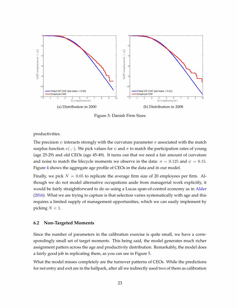
match surpluses equals its empirical counterpart of 0.51 (see Figure 3); ξ = 0.48 does the job.

The precision of normal productivity shocks (or signal) is denoted by ψ. It determines, via

equation (4), the relative importance of priors and innovations in the agents’ Bayesian updates

of their posterior mean beliefs. All else equal, a low ψ generates more volatile beliefs and

hence triggers more frequent separations, entry and exit. Moreover, it governs the rate at

which the distribution of mean beliefs converges toward the true mean-zero normal with

variance φ−1. But that it is not all. Since we exponentiate a + ǫt in the surplus technology,

the distribution of the CEO’s contribution is effectively log-normal and hence skewed.22 The

distribution of mean beliefs interacts with the skewness of effective contributions and with

the curvature parameter ρ to generate a rich pattern of participation and assignment across

22Any convex transformation of normally distributed beliefs generate such skewness. See Bolton et al. (2013)for a more detailed discussion.

22

0 1 2 3 4 5 6 7 8 9 10−12

−10

−8

−6

−4

−2

0

ln (employment)

ln(

Pr[employment>

x])

Fitted GP CDF (tail index = 0.50)Empirical CDF

(a) Distribution in 2000

0 1 2 3 4 5 6 7 8 9 10−12

−10

−8

−6

−4

−2

0

ln (employment)

ln(

Pr[employment>

x])

Fitted GP CDF (tail index = 0.51)Empirical CDF

(b) Distribution in 2008

Figure 3: Danish Firm Sizes

productivities.

The precision ψ interacts strongly with the curvature parameter σ associated with the match

surplus function x(·, ·). We pick values for ψ and σ to match the participation rates of young

(age 25-29) and old CEOs (age 45-49). It turns out that we need a fair amount of curvature

and noise to match the lifecycle moments we observe in the data: σ = 0.125 and ψ = 0.15.

Figure 4 shows the aggregate age profile of CEOs in the data and in our model.

Finally, we pick N = 0.05 to replicate the average firm size of 20 employees per firm. Al-

though we do not model alternative occupations aside from managerial work explicitly, it

would be fairly straightforward to do so using a Lucas span-of-control economy as in Alder

(2016). What we are trying to capture is that selection varies systematically with age and this

requires a limited supply of management opportunities, which we can easily implement by

picking N < 1.

6.2 Non-Targeted Moments

Since the number of parameters in the calibration exercise is quite small, we have a corre-

spondingly small set of target moments. This being said, the model generates much richer

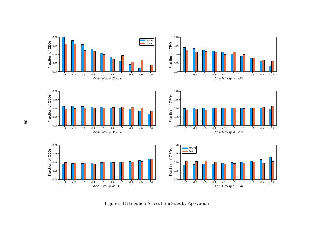
assignment patters across the age and productivity distribution. Remarkably, the model does

a fairly good job in replicating them, as you can see in Figure 5.

What the model misses completely are the turnover patterns of CEOs. While the predictions

for net entry and exit are in the ballpark, after all we indirectly used two of them as calibration

23

25-29 30-34 35-39 40-44 45-49 50-54Age Group

0.0

0.1

0.2

Fractio

n of all CE

Os

ModelData

Figure 4: Age Distribution of CEOs

targets, the gross flows are way off. We are particularly interested in transitions from one CEO

assignment to another and these are actually quite low in the data. Moreover, they follow

an inverted U-shape pattern. Young CEOs have high exit rates and don’t switch to another

executive job very often. Middle-aged managers are most likely to have a CEO spell followed

by another one while the oldest tend to stay put or exit. Moreover, the latter have very low

entry rates and the fraction of older CEOs actually drops once they are past their late 40s.

Our model generates an inverted-U-shaped transition pattern but with excessive churning

and with a fairly strong inflow of new managers even as they approach retirement. These

particular model prediction led us to introduce costly match formation in order to reduce

the rate of turnover in general and to stem the entry of fairly old mangers in particular. At

this point, the calibration is still work in progress and we only have the stylized results from

section 4.2.

7 Counterfactual Experiments

TO BE COMPLETED.

24

d.1 d.2 d.3 d.4 d.5 d.6 d.7 d.8 d.9 d.10Age Group 25-29

0.00

0.05

0.10

0.15

0.20

Frac

tion

of C

EOs Model

Data

d.1 d.2 d.3 d.4 d.5 d.6 d.7 d.8 d.9 d.10Age Group 30-34

0.00

0.05

0.10

0.15

0.20

Frac

tion

of C

EOs

d.1 d.2 d.3 d.4 d.5 d.6 d.7 d.8 d.9 d.10Age Group 35-39

0.00

0.05

0.10

0.15

0.20

Frac

tion

of C

EOs

d.1 d.2 d.3 d.4 d.5 d.6 d.7 d.8 d.9 d.10Age Group 40-44

0.00

0.05

0.10

0.15

0.20

Frac

tion

of C

EOs

d.1 d.2 d.3 d.4 d.5 d.6 d.7 d.8 d.9 d.10Age Group 45-49

0.00

0.05

0.10

0.15

0.20

Frac

tion

of C

EOs

d.1 d.2 d.3 d.4 d.5 d.6 d.7 d.8 d.9 d.10Age Group 50-54

0.00

0.05

0.10

0.15

0.20

Frac

tion

of C

EOs Model

Data

Figure 5: Distribution Across Firm Sizes by Age Group

25

8 Conclusion

TO BE COMPLETED.

26

References

ABOWD, J. M., F. KRAMARZ, AND D. N. MARGOLIS (1999): “High Wage Workers and High

Wage Firms,” Econometrica, 67, 251–333.

ALDER, S. D. (2016): “In the Wrong Hands: Complementarities, Resource Allocation, and

Aggregate TFP,” American Economic Journal: Macroeconomics, 8, 199–241.

ALDER, S. D., M. MEYER-TER VEHN, AND L. E. OHANIAN (2016): “Dynamic Sorting,” Work

in Progress.

BANDIERA, O., S. HANSEN, A. PRAT, AND R. SADUN (2017): “CEO Behavior and Firm Per-

formance,” NBER Working Paper, 1–59.

BEAUDRY, P. AND D. A. GREEN (2000): “Cohort patterns in Canadian earnings: assessing the

role of skill premia in inequality trends,” Canadian Journal of Economics, 33, 907–936.

BHATTACHARYA, D., N. GUNER, AND G. VENTURA (2013): “Distortions, Endogenous Man-

agerial Skills and Productivity Differences,” Review of Economic Dynamics, 16, 11–25.

BOLTON, P., M. K. BRUNNERMEIER, AND L. VELDKAMP (2013): “Leadership, Coordination

and Corporate Culture,” Review of Economic Studies, 80, 512–537.

EECKHOUT, J. AND P. KIRCHER (2011): “Identifying Sorting – In Theory,” Review of Economic

Studies, 78, 872–906.

EVANS, D. S. AND B. JOVANOVIC (1989): “An estimated model of entrepreneurial choice

under liquidity constraints,” Journal of Political Economy, 97, 808–827.

EVANS, D. S. AND L. S. LEIGHTON (1989): “Some empirical aspects of entrepreneurship,”

American Economic Review, 79, 519–535.

GABAIX, X. AND A. LANDIER (2008): “Why Has CEO Pay Increased So Much?” Quarterly

Journal of Economics, 123, 49–100.

GROES, F., P. KIRCHER, AND I. MANOVSKII (2015): “The U-shapes of Occupational Mobility,”

Review of Economic Studies, 82, 659–692.

GUNER, N., A. PARKHOMENKO, AND G. VENTURA (2017): “Managers and Productivity Dif-

ferences,” Working Paper, 1–64.

JOHNSON, W. R. (1978): “A theory of job shopping,” Quarterly Journal of Economics, 92,

261–278.

27

JOVANOVIC, B. (1979): “Job Matching and the Theory of Turnover,” Journal of Political Econ-

omy, 87, 972–990.

——— (2015): “Learning and Recombination,” Working Paper, 1–34.

KNIGHT, F. H. (1921): Risk, Uncertainty, and Profit, New York: Houghton Mifflin.

LINDENLAUB, I. (2016): “Sorting multi-dimensional Types: Theory and Application,” Review

of Economic Studies, forthcoming.

LISE, J., C. MEGHIR, AND J.-M. ROBIN (2013): “Mismatch, Sorting and Wage Dynamics,”

Working Paper.

LOPES DE MELO, R. (forthcoming): “Firm Wage Differentials and Labor Market Sorting: Rec-

onciling Theory and Evidence,” Journal of Political Economy, 1–32.

LUCAS, R. E. (1978): “On the Size Distribution of Business Firms,” Bell Journal of Economics,

9, 508–523.

MILLER, R. A. (1984): “Job matching and occupational choice,” Journal of Political Economy,

92, 1086–1120.

NAGYPAL, E. (2007): “Learning by doing vs. learning about match quality: Can we tell them

apart?” Review of Economic Studies, 74, 537–566.

TERVIO, M. (2008): “The Difference That CEOs Make: An Assignment Model Approach,”

American Economic Review, 98, 642–68.

28