
Faltings height and Néron-Tate height of a theta divisor · Outline Goal: studyFaltingsheightvs....
126
Faltings height and Néron-Tate height of a theta divisor Robin de Jong based on joint work with Farbod Shokrieh 3 September 2018 Intercity Seminar in Arakelov Geometry, Copenhagen
Transcript of Faltings height and Néron-Tate height of a theta divisor · Outline Goal: studyFaltingsheightvs....

Faltings height and Néron-Tate height of a thetadivisor
Robin de Jongbased on joint work with Farbod Shokrieh
3 September 2018
Intercity Seminar in Arakelov Geometry, Copenhagen

Outline
Goal: study Faltings height vs. height of a theta divisor ...
I Function field setting (good reduction)I Number field setting (good reduction)I General case (number fields)I Examples

Outline
Goal: study Faltings height vs. height of a theta divisor ...
I Function field setting (good reduction)
I Number field setting (good reduction)I General case (number fields)I Examples

Outline
Goal: study Faltings height vs. height of a theta divisor ...
I Function field setting (good reduction)I Number field setting (good reduction)
I General case (number fields)I Examples

Outline
Goal: study Faltings height vs. height of a theta divisor ...
I Function field setting (good reduction)I Number field setting (good reduction)I General case (number fields)
I Examples

Outline
Goal: study Faltings height vs. height of a theta divisor ...
I Function field setting (good reduction)I Number field setting (good reduction)I General case (number fields)I Examples

Function field setting (good reduction)
I S smooth projective connected curve over an alg. closed fieldI π : A → S abelian scheme, zero section e ∈ A(S)
I Θ symmetric effective relative Cartier divisor defining aprincipal polarization
I L = OA(Θ)
I L = Lη, A = Aη, g = dimA
I h(A) := deg e∗ΩgA/S
I L′ := L ⊗ π∗e∗L⊗−1
I h′L(Θ) := deg π∗(c1(L′)g ·Θ)/g · g !
Have π∗L = OS hence deg π∗L′ = − deg e∗L.Have π∗(c1(L′)g+1) = 0 hence deg e∗L = g · h′L(Θ).Have deg π∗L′ = −1
2h(A) by GRR / key formula.Hence h(A) = 2g · h′L(Θ).

Function field setting (good reduction)
I S smooth projective connected curve over an alg. closed field
I π : A → S abelian scheme, zero section e ∈ A(S)
I Θ symmetric effective relative Cartier divisor defining aprincipal polarization
I L = OA(Θ)
I L = Lη, A = Aη, g = dimA
I h(A) := deg e∗ΩgA/S
I L′ := L ⊗ π∗e∗L⊗−1
I h′L(Θ) := deg π∗(c1(L′)g ·Θ)/g · g !
Have π∗L = OS hence deg π∗L′ = − deg e∗L.Have π∗(c1(L′)g+1) = 0 hence deg e∗L = g · h′L(Θ).Have deg π∗L′ = −1
2h(A) by GRR / key formula.Hence h(A) = 2g · h′L(Θ).

Function field setting (good reduction)
I S smooth projective connected curve over an alg. closed fieldI π : A → S abelian scheme, zero section e ∈ A(S)
I Θ symmetric effective relative Cartier divisor defining aprincipal polarization
I L = OA(Θ)
I L = Lη, A = Aη, g = dimA
I h(A) := deg e∗ΩgA/S
I L′ := L ⊗ π∗e∗L⊗−1
I h′L(Θ) := deg π∗(c1(L′)g ·Θ)/g · g !
Have π∗L = OS hence deg π∗L′ = − deg e∗L.Have π∗(c1(L′)g+1) = 0 hence deg e∗L = g · h′L(Θ).Have deg π∗L′ = −1
2h(A) by GRR / key formula.Hence h(A) = 2g · h′L(Θ).

Function field setting (good reduction)
I S smooth projective connected curve over an alg. closed fieldI π : A → S abelian scheme, zero section e ∈ A(S)
I Θ symmetric effective relative Cartier divisor defining aprincipal polarization
I L = OA(Θ)
I L = Lη, A = Aη, g = dimA
I h(A) := deg e∗ΩgA/S
I L′ := L ⊗ π∗e∗L⊗−1
I h′L(Θ) := deg π∗(c1(L′)g ·Θ)/g · g !
Have π∗L = OS hence deg π∗L′ = − deg e∗L.
Have π∗(c1(L′)g+1) = 0 hence deg e∗L = g · h′L(Θ).Have deg π∗L′ = −1
2h(A) by GRR / key formula.Hence h(A) = 2g · h′L(Θ).
Function field setting (good reduction)
I S smooth projective connected curve over an alg. closed fieldI π : A → S abelian scheme, zero section e ∈ A(S)
I Θ symmetric effective relative Cartier divisor defining aprincipal polarization
I L = OA(Θ)
I L = Lη, A = Aη, g = dimA
I h(A) := deg e∗ΩgA/S
I L′ := L ⊗ π∗e∗L⊗−1
I h′L(Θ) := deg π∗(c1(L′)g ·Θ)/g · g !
Have π∗L = OS hence deg π∗L′ = − deg e∗L.Have π∗(c1(L′)g+1) = 0 hence deg e∗L = g · h′L(Θ).
Have deg π∗L′ = −12h(A) by GRR / key formula.
Hence h(A) = 2g · h′L(Θ).
Function field setting (good reduction)
I S smooth projective connected curve over an alg. closed fieldI π : A → S abelian scheme, zero section e ∈ A(S)
I Θ symmetric effective relative Cartier divisor defining aprincipal polarization
I L = OA(Θ)
I L = Lη, A = Aη, g = dimA
I h(A) := deg e∗ΩgA/S
I L′ := L ⊗ π∗e∗L⊗−1
I h′L(Θ) := deg π∗(c1(L′)g ·Θ)/g · g !
Have π∗L = OS hence deg π∗L′ = − deg e∗L.Have π∗(c1(L′)g+1) = 0 hence deg e∗L = g · h′L(Θ).Have deg π∗L′ = −1
2h(A) by GRR / key formula.
Hence h(A) = 2g · h′L(Θ).

Function field setting (good reduction)
I S smooth projective connected curve over an alg. closed fieldI π : A → S abelian scheme, zero section e ∈ A(S)
I Θ symmetric effective relative Cartier divisor defining aprincipal polarization
I L = OA(Θ)
I L = Lη, A = Aη, g = dimA
I h(A) := deg e∗ΩgA/S
I L′ := L ⊗ π∗e∗L⊗−1
I h′L(Θ) := deg π∗(c1(L′)g ·Θ)/g · g !
Have π∗L = OS hence deg π∗L′ = − deg e∗L.Have π∗(c1(L′)g+1) = 0 hence deg e∗L = g · h′L(Θ).Have deg π∗L′ = −1
2h(A) by GRR / key formula.Hence h(A) = 2g · h′L(Θ).

Number field setting
I k number field, d = [k : Q]
I A/k abelian variety with semistable reduction, origin e,g = dimA
I Θ symmetric effective Cartier divisor defining a principalpolarization
I L = OA(Θ)
I G connected component of Néron model over S = SpecOk
I hF (A) := deg e∗ΩgG/S/d stable Faltings height
I L′ := L⊗ e∗L⊗−1
I h′L(Θ) := 〈c1(L′)g |Θ〉/d · g · g ! Néron-Tate height of Θ
I use Zhang / Chambert-Loir / Gubler adelic admissibleintersection theory to define 〈c1(L′)g |Θ〉
Our goal: hF (A) =2g ·h′L(Θ)+d ·(a sum of local factors indexed by the places of k).
Number field setting
I k number field,
d = [k : Q]
I A/k abelian variety with semistable reduction, origin e,g = dimA
I Θ symmetric effective Cartier divisor defining a principalpolarization
I L = OA(Θ)
I G connected component of Néron model over S = SpecOk
I hF (A) := deg e∗ΩgG/S/d stable Faltings height
I L′ := L⊗ e∗L⊗−1
I h′L(Θ) := 〈c1(L′)g |Θ〉/d · g · g ! Néron-Tate height of Θ
I use Zhang / Chambert-Loir / Gubler adelic admissibleintersection theory to define 〈c1(L′)g |Θ〉
Our goal: hF (A) =2g ·h′L(Θ)+d ·(a sum of local factors indexed by the places of k).

Number field setting
I k number field, d = [k : Q]
I A/k abelian variety with semistable reduction, origin e,g = dimA
I Θ symmetric effective Cartier divisor defining a principalpolarization
I L = OA(Θ)
I G connected component of Néron model over S = SpecOk
I hF (A) := deg e∗ΩgG/S/d stable Faltings height
I L′ := L⊗ e∗L⊗−1
I h′L(Θ) := 〈c1(L′)g |Θ〉/d · g · g ! Néron-Tate height of Θ
I use Zhang / Chambert-Loir / Gubler adelic admissibleintersection theory to define 〈c1(L′)g |Θ〉
Our goal: hF (A) =2g ·h′L(Θ)+d ·(a sum of local factors indexed by the places of k).

Number field setting
I k number field, d = [k : Q]
I A/k abelian variety with semistable reduction, origin e,g = dimA
I Θ symmetric effective Cartier divisor defining a principalpolarization
I L = OA(Θ)
I G connected component of Néron model over S = SpecOk
I hF (A) := deg e∗ΩgG/S/d
stable Faltings height
I L′ := L⊗ e∗L⊗−1
I h′L(Θ) := 〈c1(L′)g |Θ〉/d · g · g ! Néron-Tate height of Θ
I use Zhang / Chambert-Loir / Gubler adelic admissibleintersection theory to define 〈c1(L′)g |Θ〉
Our goal: hF (A) =2g ·h′L(Θ)+d ·(a sum of local factors indexed by the places of k).

Number field setting
I k number field, d = [k : Q]
I A/k abelian variety with semistable reduction, origin e,g = dimA
I Θ symmetric effective Cartier divisor defining a principalpolarization
I L = OA(Θ)
I G connected component of Néron model over S = SpecOk
I hF (A) := deg e∗ΩgG/S/d stable Faltings height
I L′ := L⊗ e∗L⊗−1
I h′L(Θ) := 〈c1(L′)g |Θ〉/d · g · g ! Néron-Tate height of Θ
I use Zhang / Chambert-Loir / Gubler adelic admissibleintersection theory to define 〈c1(L′)g |Θ〉
Our goal: hF (A) =2g ·h′L(Θ)+d ·(a sum of local factors indexed by the places of k).

Number field setting
I k number field, d = [k : Q]
I A/k abelian variety with semistable reduction, origin e,g = dimA
I Θ symmetric effective Cartier divisor defining a principalpolarization
I L = OA(Θ)
I G connected component of Néron model over S = SpecOk
I hF (A) := deg e∗ΩgG/S/d stable Faltings height
I L′ := L⊗ e∗L⊗−1
I h′L(Θ) := 〈c1(L′)g |Θ〉/d · g · g !
Néron-Tate height of Θ
I use Zhang / Chambert-Loir / Gubler adelic admissibleintersection theory to define 〈c1(L′)g |Θ〉
Our goal: hF (A) =2g ·h′L(Θ)+d ·(a sum of local factors indexed by the places of k).

Number field setting
I k number field, d = [k : Q]
I A/k abelian variety with semistable reduction, origin e,g = dimA
I Θ symmetric effective Cartier divisor defining a principalpolarization
I L = OA(Θ)
I G connected component of Néron model over S = SpecOk
I hF (A) := deg e∗ΩgG/S/d stable Faltings height
I L′ := L⊗ e∗L⊗−1
I h′L(Θ) := 〈c1(L′)g |Θ〉/d · g · g ! Néron-Tate height of Θ
I use Zhang / Chambert-Loir / Gubler adelic admissibleintersection theory to define 〈c1(L′)g |Θ〉
Our goal: hF (A) =2g ·h′L(Θ)+d ·(a sum of local factors indexed by the places of k).

Number field setting
I k number field, d = [k : Q]
I A/k abelian variety with semistable reduction, origin e,g = dimA
I Θ symmetric effective Cartier divisor defining a principalpolarization
I L = OA(Θ)
I G connected component of Néron model over S = SpecOk
I hF (A) := deg e∗ΩgG/S/d stable Faltings height
I L′ := L⊗ e∗L⊗−1
I h′L(Θ) := 〈c1(L′)g |Θ〉/d · g · g ! Néron-Tate height of Θ
I use Zhang / Chambert-Loir / Gubler adelic admissibleintersection theory to define 〈c1(L′)g |Θ〉
Our goal: hF (A) =2g ·h′L(Θ)+d ·(a sum of local factors indexed by the places of k).

Case of good reduction
First case: A/k has everywhere good reduction. Expect onlycontributions from the infinite places.
I A complex abelian varietyI Θ symmetric effective Cartier divisor defining a principal
polarization λ : A ∼−→ At
I L = OA(Θ)
I endow L with admissible smooth hermitian metric ‖ · ‖ (iec1(L) is translation-invariant)
I choose s ∈ H0(A,L) non-zeroI put I (A, λ) := −
∫A log ‖s‖ dµH + 1
2 log∫A ‖s‖
2 dµHI where µH Haar measure on A normalized to give A unit
volumeI note I (A, λ) > 0.

Case of good reduction
First case: A/k has everywhere good reduction.
Expect onlycontributions from the infinite places.
I A complex abelian varietyI Θ symmetric effective Cartier divisor defining a principal
polarization λ : A ∼−→ At
I L = OA(Θ)
I endow L with admissible smooth hermitian metric ‖ · ‖ (iec1(L) is translation-invariant)
I choose s ∈ H0(A,L) non-zeroI put I (A, λ) := −
∫A log ‖s‖ dµH + 1
2 log∫A ‖s‖
2 dµHI where µH Haar measure on A normalized to give A unit
volumeI note I (A, λ) > 0.

Case of good reduction
First case: A/k has everywhere good reduction. Expect onlycontributions from the infinite places.
I A complex abelian varietyI Θ symmetric effective Cartier divisor defining a principal
polarization λ : A ∼−→ At
I L = OA(Θ)
I endow L with admissible smooth hermitian metric ‖ · ‖ (iec1(L) is translation-invariant)
I choose s ∈ H0(A,L) non-zeroI put I (A, λ) := −
∫A log ‖s‖ dµH + 1
2 log∫A ‖s‖
2 dµHI where µH Haar measure on A normalized to give A unit
volumeI note I (A, λ) > 0.

Case of good reduction
First case: A/k has everywhere good reduction. Expect onlycontributions from the infinite places.
I A complex abelian variety
I Θ symmetric effective Cartier divisor defining a principalpolarization λ : A ∼−→ At
I L = OA(Θ)
I endow L with admissible smooth hermitian metric ‖ · ‖ (iec1(L) is translation-invariant)
I choose s ∈ H0(A,L) non-zeroI put I (A, λ) := −
∫A log ‖s‖ dµH + 1
2 log∫A ‖s‖
2 dµHI where µH Haar measure on A normalized to give A unit
volumeI note I (A, λ) > 0.

Case of good reduction
First case: A/k has everywhere good reduction. Expect onlycontributions from the infinite places.
I A complex abelian varietyI Θ symmetric effective Cartier divisor defining a principal
polarization λ : A ∼−→ At
I L = OA(Θ)
I endow L with admissible smooth hermitian metric ‖ · ‖ (iec1(L) is translation-invariant)
I choose s ∈ H0(A,L) non-zeroI put I (A, λ) := −
∫A log ‖s‖ dµH + 1
2 log∫A ‖s‖
2 dµHI where µH Haar measure on A normalized to give A unit
volumeI note I (A, λ) > 0.

Case of good reduction
First case: A/k has everywhere good reduction. Expect onlycontributions from the infinite places.
I A complex abelian varietyI Θ symmetric effective Cartier divisor defining a principal
polarization λ : A ∼−→ At
I L = OA(Θ)
I endow L with admissible smooth hermitian metric ‖ · ‖ (iec1(L) is translation-invariant)
I choose s ∈ H0(A,L) non-zero
I put I (A, λ) := −∫A log ‖s‖ dµH + 1
2 log∫A ‖s‖
2 dµHI where µH Haar measure on A normalized to give A unit
volumeI note I (A, λ) > 0.
Case of good reduction
First case: A/k has everywhere good reduction. Expect onlycontributions from the infinite places.
I A complex abelian varietyI Θ symmetric effective Cartier divisor defining a principal
polarization λ : A ∼−→ At
I L = OA(Θ)
I endow L with admissible smooth hermitian metric ‖ · ‖ (iec1(L) is translation-invariant)
I choose s ∈ H0(A,L) non-zeroI put I (A, λ) := −
∫A log ‖s‖ dµH + 1
2 log∫A ‖s‖
2 dµH
I where µH Haar measure on A normalized to give A unitvolume
I note I (A, λ) > 0.

Case of good reduction
First case: A/k has everywhere good reduction. Expect onlycontributions from the infinite places.
I A complex abelian varietyI Θ symmetric effective Cartier divisor defining a principal
polarization λ : A ∼−→ At
I L = OA(Θ)
I endow L with admissible smooth hermitian metric ‖ · ‖ (iec1(L) is translation-invariant)
I choose s ∈ H0(A,L) non-zeroI put I (A, λ) := −
∫A log ‖s‖ dµH + 1
2 log∫A ‖s‖
2 dµHI where µH Haar measure on A normalized to give A unit
volume
I note I (A, λ) > 0.

Case of good reduction
First case: A/k has everywhere good reduction. Expect onlycontributions from the infinite places.
I A complex abelian varietyI Θ symmetric effective Cartier divisor defining a principal
polarization λ : A ∼−→ At
I L = OA(Θ)
I endow L with admissible smooth hermitian metric ‖ · ‖ (iec1(L) is translation-invariant)
I choose s ∈ H0(A,L) non-zeroI put I (A, λ) := −
∫A log ‖s‖ dµH + 1
2 log∫A ‖s‖
2 dµHI where µH Haar measure on A normalized to give A unit
volumeI note I (A, λ) > 0.

Case of good reduction
Hindry and Autissier have shown:
assume A/k has everywheregood reduction. Then
hF (A) = 2g · h′L(Θ)− κ0 g +2d
∑v∈M(k)∞
I (Av , λv ) .
Here
I κ0 = log(π√2), related to ‖α‖2Fa =
√−1g
2
2g∫A α ∧ α
I M(k)∞ = set of complex embeddings of kProof: application of ARR / key formula.What about the general case?

Case of good reduction
Hindry and Autissier have shown: assume A/k has everywheregood reduction. Then
hF (A) = 2g · h′L(Θ)− κ0 g +2d
∑v∈M(k)∞
I (Av , λv ) .
Here
I κ0 = log(π√2), related to ‖α‖2Fa =
√−1g
2
2g∫A α ∧ α
I M(k)∞ = set of complex embeddings of k
Proof: application of ARR / key formula.What about the general case?

Case of good reduction
Hindry and Autissier have shown: assume A/k has everywheregood reduction. Then
hF (A) = 2g · h′L(Θ)− κ0 g +2d
∑v∈M(k)∞
I (Av , λv ) .
Here
I κ0 = log(π√2), related to ‖α‖2Fa =
√−1g
2
2g∫A α ∧ α
I M(k)∞ = set of complex embeddings of kProof: application of ARR / key formula.
What about the general case?

Case of good reduction
Hindry and Autissier have shown: assume A/k has everywheregood reduction. Then
hF (A) = 2g · h′L(Θ)− κ0 g +2d
∑v∈M(k)∞
I (Av , λv ) .
Here
I κ0 = log(π√2), related to ‖α‖2Fa =
√−1g
2
2g∫A α ∧ α
I M(k)∞ = set of complex embeddings of kProof: application of ARR / key formula.What about the general case?

Non-archimedean uniformization
I (A, λ) principally polarized abelian variety over F , fractionfield of a complete discrete valuation ring R
I assume A has split semistable reductionI get 1→ T → G → B → 0 over R with T = Gr
m split torus, Babelian scheme over R
I set X := Hom(T ,Gm), Y := Hom(T t ,Gm), principalpolarization gives φ : Y
∼−→ X
I have natural maps Ω: X → Bt , Ω′ : Y → B
I and a trivialization of the restriction to the generic fiber of thepullback of the Poincaré bundle to Y × X
I this gives a bilinear map b : Y × X → Z with b(·, φ(·))positive definite
I the real torus Σ = Hom(X ,R)/Y is a principally polarizedtropical abelian variety canonically associated to (A, λ)
Non-archimedean uniformization
I (A, λ) principally polarized abelian variety over F , fractionfield of a complete discrete valuation ring R
I assume A has split semistable reduction
I get 1→ T → G → B → 0 over R with T = Grm split torus, B
abelian scheme over RI set X := Hom(T ,Gm), Y := Hom(T t ,Gm), principal
polarization gives φ : Y∼−→ X
I have natural maps Ω: X → Bt , Ω′ : Y → B
I and a trivialization of the restriction to the generic fiber of thepullback of the Poincaré bundle to Y × X
I this gives a bilinear map b : Y × X → Z with b(·, φ(·))positive definite
I the real torus Σ = Hom(X ,R)/Y is a principally polarizedtropical abelian variety canonically associated to (A, λ)

Non-archimedean uniformization
I (A, λ) principally polarized abelian variety over F , fractionfield of a complete discrete valuation ring R
I assume A has split semistable reductionI get 1→ T → G → B → 0 over R with T = Gr
m split torus, Babelian scheme over R
I set X := Hom(T ,Gm), Y := Hom(T t ,Gm), principalpolarization gives φ : Y
∼−→ X
I have natural maps Ω: X → Bt , Ω′ : Y → B
I and a trivialization of the restriction to the generic fiber of thepullback of the Poincaré bundle to Y × X
I this gives a bilinear map b : Y × X → Z with b(·, φ(·))positive definite
I the real torus Σ = Hom(X ,R)/Y is a principally polarizedtropical abelian variety canonically associated to (A, λ)

Tropical abelian varieties
A principally polarized tropical abelian variety is a real torusΣ = Hom(X ,R)/Y where Y ,X is a pair of finitely generated freeabelian groups together with an isomorphism φ : Y
∼−→ X and abilinear map b : Y × X → Z such that b(·, φ(·)) is positive definite.
We get an induced norm ‖ · ‖ on V = Hom(X ,R).
We have the Voronoi polytope with center the origin
Vor(0) =
ν ∈ V
∣∣∣∣ ‖ν‖ = minv ′∈Y
‖ν − v ′‖
as a rational polytope in V .
The tropical moment of Σ = V /Y is the value of the integral∫Vor(0)
‖ν‖2 dµL(ν) .
Here µL denotes the Lebesgue measure on V , normalized to giveVor(0) unit volume.

Tropical moment
Alternatively, consider the tropical Riemann theta function
Ψ(ν) := minu′∈Y
12‖u′‖2 + [ν, u′]
(1)
for ν ∈ V . The function Ψ is piecewise affine on V . The modifiedRiemann theta function
‖Ψ‖(ν) := Ψ(ν) +12‖ν‖2 (2)
on V is Y -invariant and hence descends to Σ. Explicitly
‖Ψ‖(ν) =12minu′∈Y
‖ν + u′‖2
for all ν ∈ V . The tropical moment of Σ can alternatively bewritten as
2∫
Σ‖Ψ‖ dµH ,
where µH is the Haar measure on Σ, normalized to give Σ unitvolume. It is a non-negative rational number, zero iff Σ = (0).
Tropical moment
Alternatively, consider the tropical Riemann theta function
Ψ(ν) := minu′∈Y
12‖u′‖2 + [ν, u′]
(1)
for ν ∈ V .
The function Ψ is piecewise affine on V . The modifiedRiemann theta function
‖Ψ‖(ν) := Ψ(ν) +12‖ν‖2 (2)
on V is Y -invariant and hence descends to Σ. Explicitly
‖Ψ‖(ν) =12minu′∈Y
‖ν + u′‖2
for all ν ∈ V . The tropical moment of Σ can alternatively bewritten as
2∫
Σ‖Ψ‖ dµH ,
where µH is the Haar measure on Σ, normalized to give Σ unitvolume. It is a non-negative rational number, zero iff Σ = (0).

Tropical moment
Alternatively, consider the tropical Riemann theta function
Ψ(ν) := minu′∈Y
12‖u′‖2 + [ν, u′]
(1)
for ν ∈ V . The function Ψ is piecewise affine on V .
The modifiedRiemann theta function
‖Ψ‖(ν) := Ψ(ν) +12‖ν‖2 (2)
on V is Y -invariant and hence descends to Σ. Explicitly
‖Ψ‖(ν) =12minu′∈Y
‖ν + u′‖2
for all ν ∈ V . The tropical moment of Σ can alternatively bewritten as
2∫
Σ‖Ψ‖ dµH ,
where µH is the Haar measure on Σ, normalized to give Σ unitvolume. It is a non-negative rational number, zero iff Σ = (0).

Tropical moment
Alternatively, consider the tropical Riemann theta function
Ψ(ν) := minu′∈Y
12‖u′‖2 + [ν, u′]
(1)
for ν ∈ V . The function Ψ is piecewise affine on V . The modifiedRiemann theta function
‖Ψ‖(ν) := Ψ(ν) +12‖ν‖2 (2)
on V is Y -invariant and hence descends to Σ.
Explicitly
‖Ψ‖(ν) =12minu′∈Y
‖ν + u′‖2
for all ν ∈ V . The tropical moment of Σ can alternatively bewritten as
2∫
Σ‖Ψ‖ dµH ,
where µH is the Haar measure on Σ, normalized to give Σ unitvolume. It is a non-negative rational number, zero iff Σ = (0).

Tropical moment
Alternatively, consider the tropical Riemann theta function
Ψ(ν) := minu′∈Y
12‖u′‖2 + [ν, u′]
(1)
for ν ∈ V . The function Ψ is piecewise affine on V . The modifiedRiemann theta function
‖Ψ‖(ν) := Ψ(ν) +12‖ν‖2 (2)
on V is Y -invariant and hence descends to Σ. Explicitly
‖Ψ‖(ν) =12minu′∈Y
‖ν + u′‖2
for all ν ∈ V .
The tropical moment of Σ can alternatively bewritten as
2∫
Σ‖Ψ‖ dµH ,
where µH is the Haar measure on Σ, normalized to give Σ unitvolume. It is a non-negative rational number, zero iff Σ = (0).

Tropical moment
Alternatively, consider the tropical Riemann theta function
Ψ(ν) := minu′∈Y
12‖u′‖2 + [ν, u′]
(1)
for ν ∈ V . The function Ψ is piecewise affine on V . The modifiedRiemann theta function
‖Ψ‖(ν) := Ψ(ν) +12‖ν‖2 (2)
on V is Y -invariant and hence descends to Σ. Explicitly
‖Ψ‖(ν) =12minu′∈Y
‖ν + u′‖2
for all ν ∈ V . The tropical moment of Σ can alternatively bewritten as
2∫
Σ‖Ψ‖ dµH ,
where µH is the Haar measure on Σ, normalized to give Σ unitvolume. It is a non-negative rational number, zero iff Σ = (0).

General case
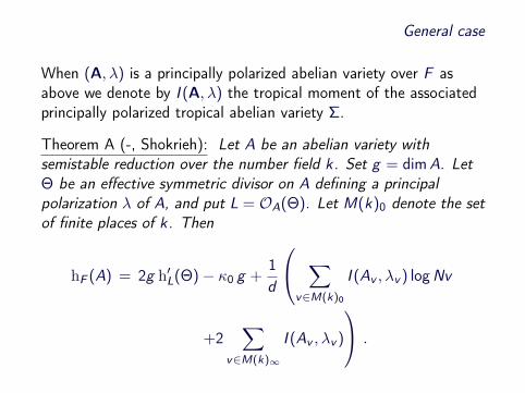
When (A, λ) is a principally polarized abelian variety over F asabove we denote by I (A, λ) the tropical moment of the associatedprincipally polarized tropical abelian variety Σ.
Theorem A (-, Shokrieh): Let A be an abelian variety withsemistable reduction over the number field k . Set g = dimA. LetΘ be an effective symmetric divisor on A defining a principalpolarization λ of A, and put L = OA(Θ). Let M(k)0 denote the setof finite places of k . Then
hF (A) = 2g h′L(Θ)− κ0 g +1d
∑v∈M(k)0
I (Av , λv ) logNv
+2∑
v∈M(k)∞
I (Av , λv )
.

General case
When (A, λ) is a principally polarized abelian variety over F asabove we denote by I (A, λ) the tropical moment of the associatedprincipally polarized tropical abelian variety Σ.
Theorem A (-, Shokrieh): Let A be an abelian variety withsemistable reduction over the number field k . Set g = dimA. LetΘ be an effective symmetric divisor on A defining a principalpolarization λ of A, and put L = OA(Θ). Let M(k)0 denote the setof finite places of k . Then
hF (A) = 2g h′L(Θ)− κ0 g +1d
∑v∈M(k)0
I (Av , λv ) logNv
+2∑
v∈M(k)∞
I (Av , λv )
.
General case
When (A, λ) is a principally polarized abelian variety over F asabove we denote by I (A, λ) the tropical moment of the associatedprincipally polarized tropical abelian variety Σ.
Theorem A (-, Shokrieh): Let A be an abelian variety withsemistable reduction over the number field k .
Set g = dimA. LetΘ be an effective symmetric divisor on A defining a principalpolarization λ of A, and put L = OA(Θ). Let M(k)0 denote the setof finite places of k . Then
hF (A) = 2g h′L(Θ)− κ0 g +1d
∑v∈M(k)0
I (Av , λv ) logNv
+2∑
v∈M(k)∞
I (Av , λv )
.

General case
When (A, λ) is a principally polarized abelian variety over F asabove we denote by I (A, λ) the tropical moment of the associatedprincipally polarized tropical abelian variety Σ.
Theorem A (-, Shokrieh): Let A be an abelian variety withsemistable reduction over the number field k . Set g = dimA.
LetΘ be an effective symmetric divisor on A defining a principalpolarization λ of A, and put L = OA(Θ). Let M(k)0 denote the setof finite places of k . Then
hF (A) = 2g h′L(Θ)− κ0 g +1d
∑v∈M(k)0
I (Av , λv ) logNv
+2∑
v∈M(k)∞
I (Av , λv )
.

General case
When (A, λ) is a principally polarized abelian variety over F asabove we denote by I (A, λ) the tropical moment of the associatedprincipally polarized tropical abelian variety Σ.
Theorem A (-, Shokrieh): Let A be an abelian variety withsemistable reduction over the number field k . Set g = dimA. LetΘ be an effective symmetric divisor on A defining a principalpolarization λ of A, and put L = OA(Θ).
Let M(k)0 denote the setof finite places of k . Then
hF (A) = 2g h′L(Θ)− κ0 g +1d
∑v∈M(k)0
I (Av , λv ) logNv
+2∑
v∈M(k)∞
I (Av , λv )
.

General case
When (A, λ) is a principally polarized abelian variety over F asabove we denote by I (A, λ) the tropical moment of the associatedprincipally polarized tropical abelian variety Σ.
Theorem A (-, Shokrieh): Let A be an abelian variety withsemistable reduction over the number field k . Set g = dimA. LetΘ be an effective symmetric divisor on A defining a principalpolarization λ of A, and put L = OA(Θ). Let M(k)0 denote the setof finite places of k .
Then
hF (A) = 2g h′L(Θ)− κ0 g +1d
∑v∈M(k)0
I (Av , λv ) logNv
+2∑
v∈M(k)∞
I (Av , λv )
.
General case
When (A, λ) is a principally polarized abelian variety over F asabove we denote by I (A, λ) the tropical moment of the associatedprincipally polarized tropical abelian variety Σ.
Theorem A (-, Shokrieh): Let A be an abelian variety withsemistable reduction over the number field k . Set g = dimA. LetΘ be an effective symmetric divisor on A defining a principalpolarization λ of A, and put L = OA(Θ). Let M(k)0 denote the setof finite places of k . Then
hF (A) = 2g h′L(Θ)− κ0 g +1d
∑v∈M(k)0
I (Av , λv ) logNv
+2∑
v∈M(k)∞
I (Av , λv )
.

General case
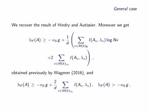
We recover the result of Hindry and Autissier. Moreover we get
hF (A) ≥ − κ0 g +1d
∑v∈M(k)0
I (Av , λv ) logNv
+2∑
v∈M(k)∞
I (Av , λv )
,
obtained previously by Wagener (2016), and
hF (A) ≥ −κ0 g +2d
∑v∈M(k)∞
I (Av , λv ) , hF (A) > −κ0 g ,
previously obtained by Bost (1996).

General case
We recover the result of Hindry and Autissier. Moreover we get
hF (A) ≥ − κ0 g +1d
∑v∈M(k)0
I (Av , λv ) logNv
+2∑
v∈M(k)∞
I (Av , λv )
,
obtained previously by Wagener (2016), and
hF (A) ≥ −κ0 g +2d
∑v∈M(k)∞
I (Av , λv ) , hF (A) > −κ0 g ,
previously obtained by Bost (1996).

General case
We recover the result of Hindry and Autissier. Moreover we get
hF (A) ≥ − κ0 g +1d
∑v∈M(k)0
I (Av , λv ) logNv
+2∑
v∈M(k)∞
I (Av , λv )
,
obtained previously by Wagener (2016),
and
hF (A) ≥ −κ0 g +2d
∑v∈M(k)∞
I (Av , λv ) , hF (A) > −κ0 g ,
previously obtained by Bost (1996).

General case
We recover the result of Hindry and Autissier. Moreover we get
hF (A) ≥ − κ0 g +1d
∑v∈M(k)0
I (Av , λv ) logNv
+2∑
v∈M(k)∞
I (Av , λv )
,
obtained previously by Wagener (2016), and
hF (A) ≥ −κ0 g +2d
∑v∈M(k)∞
I (Av , λv ) ,
hF (A) > −κ0 g ,
previously obtained by Bost (1996).
General case
We recover the result of Hindry and Autissier. Moreover we get
hF (A) ≥ − κ0 g +1d
∑v∈M(k)0
I (Av , λv ) logNv
+2∑
v∈M(k)∞
I (Av , λv )
,
obtained previously by Wagener (2016), and
hF (A) ≥ −κ0 g +2d
∑v∈M(k)∞
I (Av , λv ) , hF (A) > −κ0 g ,
previously obtained by Bost (1996).

General case
We recover the result of Hindry and Autissier. Moreover we get
hF (A) ≥ − κ0 g +1d
∑v∈M(k)0
I (Av , λv ) logNv
+2∑
v∈M(k)∞
I (Av , λv )
,
obtained previously by Wagener (2016), and
hF (A) ≥ −κ0 g +2d
∑v∈M(k)∞
I (Av , λv ) , hF (A) > −κ0 g ,
previously obtained by Bost (1996).

General case
Side remark: in the function field setting with semistable reductionwe obtain
h(A) = 2g h′L(Θ) +∑v∈S0
I (Av , λv )
with S0 the set of closed points of S .
This refines the well-knownfact (Moret-Bailly, Szpiro, Faltings-Chai) that h(A) ≥ 0.

General case
Side remark: in the function field setting with semistable reductionwe obtain
h(A) = 2g h′L(Θ) +∑v∈S0
I (Av , λv )
with S0 the set of closed points of S . This refines the well-knownfact (Moret-Bailly, Szpiro, Faltings-Chai) that h(A) ≥ 0.

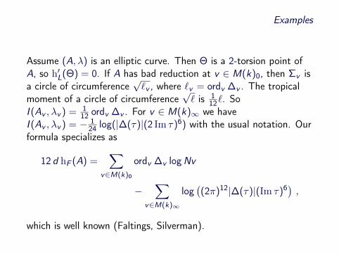
Examples
Assume (A, λ) is an elliptic curve. Then Θ is a 2-torsion point ofA, so h′L(Θ) = 0. If A has bad reduction at v ∈ M(k)0, then Σv isa circle of circumference
√`v , where `v = ordv ∆v . The tropical
moment of a circle of circumference√` is 1
12`. SoI (Av , λv ) = 1
12 ordv ∆v . For v ∈ M(k)∞ we haveI (Av , λv ) = − 1
24 log(|∆(τ)|(2 Im τ)6) with the usual notation. Ourformula specializes as
12 d hF (A) =∑
v∈M(k)0
ordv ∆v logNv
−∑
v∈M(k)∞
log((2π)12|∆(τ)|(Im τ)6) ,
which is well known (Faltings, Silverman).

Examples
Assume (A, λ) is an elliptic curve.
Then Θ is a 2-torsion point ofA, so h′L(Θ) = 0. If A has bad reduction at v ∈ M(k)0, then Σv isa circle of circumference
√`v , where `v = ordv ∆v . The tropical
moment of a circle of circumference√` is 1
12`. SoI (Av , λv ) = 1
12 ordv ∆v . For v ∈ M(k)∞ we haveI (Av , λv ) = − 1
24 log(|∆(τ)|(2 Im τ)6) with the usual notation. Ourformula specializes as
12 d hF (A) =∑
v∈M(k)0
ordv ∆v logNv
−∑
v∈M(k)∞
log((2π)12|∆(τ)|(Im τ)6) ,
which is well known (Faltings, Silverman).

Examples
Assume (A, λ) is an elliptic curve. Then Θ is a 2-torsion point ofA, so h′L(Θ) = 0.
If A has bad reduction at v ∈ M(k)0, then Σv isa circle of circumference
√`v , where `v = ordv ∆v . The tropical
moment of a circle of circumference√` is 1
12`. SoI (Av , λv ) = 1
12 ordv ∆v . For v ∈ M(k)∞ we haveI (Av , λv ) = − 1
24 log(|∆(τ)|(2 Im τ)6) with the usual notation. Ourformula specializes as
12 d hF (A) =∑
v∈M(k)0
ordv ∆v logNv
−∑
v∈M(k)∞
log((2π)12|∆(τ)|(Im τ)6) ,
which is well known (Faltings, Silverman).

Examples
Assume (A, λ) is an elliptic curve. Then Θ is a 2-torsion point ofA, so h′L(Θ) = 0. If A has bad reduction at v ∈ M(k)0, then Σv isa circle of circumference
√`v , where `v = ordv ∆v .
The tropicalmoment of a circle of circumference
√` is 1
12`. SoI (Av , λv ) = 1
12 ordv ∆v . For v ∈ M(k)∞ we haveI (Av , λv ) = − 1
24 log(|∆(τ)|(2 Im τ)6) with the usual notation. Ourformula specializes as
12 d hF (A) =∑
v∈M(k)0
ordv ∆v logNv
−∑
v∈M(k)∞
log((2π)12|∆(τ)|(Im τ)6) ,
which is well known (Faltings, Silverman).

Examples
Assume (A, λ) is an elliptic curve. Then Θ is a 2-torsion point ofA, so h′L(Θ) = 0. If A has bad reduction at v ∈ M(k)0, then Σv isa circle of circumference
√`v , where `v = ordv ∆v . The tropical
moment of a circle of circumference√` is 1
12`.
SoI (Av , λv ) = 1
12 ordv ∆v . For v ∈ M(k)∞ we haveI (Av , λv ) = − 1
24 log(|∆(τ)|(2 Im τ)6) with the usual notation. Ourformula specializes as
12 d hF (A) =∑
v∈M(k)0
ordv ∆v logNv
−∑
v∈M(k)∞
log((2π)12|∆(τ)|(Im τ)6) ,
which is well known (Faltings, Silverman).

Examples
Assume (A, λ) is an elliptic curve. Then Θ is a 2-torsion point ofA, so h′L(Θ) = 0. If A has bad reduction at v ∈ M(k)0, then Σv isa circle of circumference
√`v , where `v = ordv ∆v . The tropical
moment of a circle of circumference√` is 1
12`. SoI (Av , λv ) = 1
12 ordv ∆v .
For v ∈ M(k)∞ we haveI (Av , λv ) = − 1
24 log(|∆(τ)|(2 Im τ)6) with the usual notation. Ourformula specializes as
12 d hF (A) =∑
v∈M(k)0
ordv ∆v logNv
−∑
v∈M(k)∞
log((2π)12|∆(τ)|(Im τ)6) ,
which is well known (Faltings, Silverman).

Examples
Assume (A, λ) is an elliptic curve. Then Θ is a 2-torsion point ofA, so h′L(Θ) = 0. If A has bad reduction at v ∈ M(k)0, then Σv isa circle of circumference
√`v , where `v = ordv ∆v . The tropical
moment of a circle of circumference√` is 1
12`. SoI (Av , λv ) = 1
12 ordv ∆v . For v ∈ M(k)∞ we haveI (Av , λv ) = − 1
24 log(|∆(τ)|(2 Im τ)6) with the usual notation.
Ourformula specializes as
12 d hF (A) =∑
v∈M(k)0
ordv ∆v logNv
−∑
v∈M(k)∞
log((2π)12|∆(τ)|(Im τ)6) ,
which is well known (Faltings, Silverman).
Examples
Assume (A, λ) is an elliptic curve. Then Θ is a 2-torsion point ofA, so h′L(Θ) = 0. If A has bad reduction at v ∈ M(k)0, then Σv isa circle of circumference
√`v , where `v = ordv ∆v . The tropical
moment of a circle of circumference√` is 1
12`. SoI (Av , λv ) = 1
12 ordv ∆v . For v ∈ M(k)∞ we haveI (Av , λv ) = − 1
24 log(|∆(τ)|(2 Im τ)6) with the usual notation. Ourformula specializes as
12 d hF (A) =∑
v∈M(k)0
ordv ∆v logNv
−∑
v∈M(k)∞
log((2π)12|∆(τ)|(Im τ)6) ,
which is well known (Faltings, Silverman).
Examples
Let C be a smooth projective geometrically connected curve withsemistable reduction over the number field k .
Let (A, λ) be itsjacobian. Let Γv be the dual graph of the geometric special fiber ofthe stable model of C at v , endowed with its canonical metricstructure. For example, Γv is connected, and the total length `(Γv )equals the number of singular points in the geometric special fiber.Can we relate I (Av , λv ) for v ∈ M(k)0 to combinatorial invariantsof the metric graph Γv associated to C at v?
Examples
Let C be a smooth projective geometrically connected curve withsemistable reduction over the number field k . Let (A, λ) be itsjacobian.
Let Γv be the dual graph of the geometric special fiber ofthe stable model of C at v , endowed with its canonical metricstructure. For example, Γv is connected, and the total length `(Γv )equals the number of singular points in the geometric special fiber.Can we relate I (Av , λv ) for v ∈ M(k)0 to combinatorial invariantsof the metric graph Γv associated to C at v?
Examples
Let C be a smooth projective geometrically connected curve withsemistable reduction over the number field k . Let (A, λ) be itsjacobian. Let Γv be the dual graph of the geometric special fiber ofthe stable model of C at v , endowed with its canonical metricstructure.
For example, Γv is connected, and the total length `(Γv )equals the number of singular points in the geometric special fiber.Can we relate I (Av , λv ) for v ∈ M(k)0 to combinatorial invariantsof the metric graph Γv associated to C at v?

Examples
Let C be a smooth projective geometrically connected curve withsemistable reduction over the number field k . Let (A, λ) be itsjacobian. Let Γv be the dual graph of the geometric special fiber ofthe stable model of C at v , endowed with its canonical metricstructure. For example, Γv is connected, and the total length `(Γv )equals the number of singular points in the geometric special fiber.
Can we relate I (Av , λv ) for v ∈ M(k)0 to combinatorial invariantsof the metric graph Γv associated to C at v?

Examples
Let C be a smooth projective geometrically connected curve withsemistable reduction over the number field k . Let (A, λ) be itsjacobian. Let Γv be the dual graph of the geometric special fiber ofthe stable model of C at v , endowed with its canonical metricstructure. For example, Γv is connected, and the total length `(Γv )equals the number of singular points in the geometric special fiber.Can we relate I (Av , λv ) for v ∈ M(k)0 to combinatorial invariantsof the metric graph Γv associated to C at v?

Examples
Let Γ be a connected metric graph. Let r(p, q) denote the effectiveresistance between points p, q ∈ Γ.
Fix q ∈ Γ and setf (x) = 1
2 r(x , q). We set (cf. Baker-Rumely, Chinburg-Rumely)
τ(Γ) :=
∫Γ(f ′(x))2 d x =
∫Γf ∆f .
Then τ(Γ) is independent of the choice of q.

Examples
Let Γ be a connected metric graph. Let r(p, q) denote the effectiveresistance between points p, q ∈ Γ. Fix q ∈ Γ and setf (x) = 1
2 r(x , q).
We set (cf. Baker-Rumely, Chinburg-Rumely)
τ(Γ) :=
∫Γ(f ′(x))2 d x =
∫Γf ∆f .
Then τ(Γ) is independent of the choice of q.

Examples
Let Γ be a connected metric graph. Let r(p, q) denote the effectiveresistance between points p, q ∈ Γ. Fix q ∈ Γ and setf (x) = 1
2 r(x , q). We set (cf. Baker-Rumely, Chinburg-Rumely)
τ(Γ) :=
∫Γ(f ′(x))2 d x =
∫Γf ∆f .
Then τ(Γ) is independent of the choice of q.

Examples
Let Γ be a connected metric graph. Let r(p, q) denote the effectiveresistance between points p, q ∈ Γ. Fix q ∈ Γ and setf (x) = 1
2 r(x , q). We set (cf. Baker-Rumely, Chinburg-Rumely)
τ(Γ) :=
∫Γ(f ′(x))2 d x =
∫Γf ∆f .
Then τ(Γ) is independent of the choice of q.

Examples
Let G be a model of Γ, and fix an orientation on G . We then havea natural boundary map ∂ : C1(G ,Z)→ C0(G ,Z) with kernelH1(G ,Z).
The space C1(G ,R) has a natural inner productdetermined by edge-lengths, i.e. [ei , ej ] = `(ei )δij . The Hilbertsubspace H1(G ,R) is an invariant of Γ, as is the latticeY := H1(G ,Z) in it.
Let X = Y and b : Y × X → Z the restriction of [·, ·] to Y × Y .We obtain a principally polarized tropical abelian varietyΣ = Hom(X ,R)/Y from Γ called the tropical jacobian of Γ.

Examples
Let G be a model of Γ, and fix an orientation on G . We then havea natural boundary map ∂ : C1(G ,Z)→ C0(G ,Z) with kernelH1(G ,Z). The space C1(G ,R) has a natural inner productdetermined by edge-lengths, i.e. [ei , ej ] = `(ei )δij .
The Hilbertsubspace H1(G ,R) is an invariant of Γ, as is the latticeY := H1(G ,Z) in it.
Let X = Y and b : Y × X → Z the restriction of [·, ·] to Y × Y .We obtain a principally polarized tropical abelian varietyΣ = Hom(X ,R)/Y from Γ called the tropical jacobian of Γ.

Examples
Let G be a model of Γ, and fix an orientation on G . We then havea natural boundary map ∂ : C1(G ,Z)→ C0(G ,Z) with kernelH1(G ,Z). The space C1(G ,R) has a natural inner productdetermined by edge-lengths, i.e. [ei , ej ] = `(ei )δij . The Hilbertsubspace H1(G ,R) is an invariant of Γ, as is the latticeY := H1(G ,Z) in it.
Let X = Y and b : Y × X → Z the restriction of [·, ·] to Y × Y .
We obtain a principally polarized tropical abelian varietyΣ = Hom(X ,R)/Y from Γ called the tropical jacobian of Γ.

Examples
Let G be a model of Γ, and fix an orientation on G . We then havea natural boundary map ∂ : C1(G ,Z)→ C0(G ,Z) with kernelH1(G ,Z). The space C1(G ,R) has a natural inner productdetermined by edge-lengths, i.e. [ei , ej ] = `(ei )δij . The Hilbertsubspace H1(G ,R) is an invariant of Γ, as is the latticeY := H1(G ,Z) in it.
Let X = Y and b : Y × X → Z the restriction of [·, ·] to Y × Y .We obtain a principally polarized tropical abelian varietyΣ = Hom(X ,R)/Y from Γ called the tropical jacobian of Γ.

Examples
Theorem (-, Shokrieh): Let I (Γ) denote the tropical moment of thetropical jacobian of Γ. Then the relation
I (Γ) =18`(Γ)− 1
2τ(Γ)
holds. Here `(Γ) is the total length of Γ, and τ(Γ) its tau-invariant.
Side remark: this allows fast computation of I (Γ), starting from thediscrete Laplacian on a model G . Only need to perform a couple ofmatrix multiplications and Gauss eliminations where the matricesinvolved have size |V (G )|. Computation of tropical moment ofgeneral lattices is expected by (some) experts to be NP-hard.

Examples
Theorem (-, Shokrieh): Let I (Γ) denote the tropical moment of thetropical jacobian of Γ. Then the relation
I (Γ) =18`(Γ)− 1
2τ(Γ)
holds. Here `(Γ) is the total length of Γ, and τ(Γ) its tau-invariant.
Side remark: this allows fast computation of I (Γ), starting from thediscrete Laplacian on a model G .
Only need to perform a couple ofmatrix multiplications and Gauss eliminations where the matricesinvolved have size |V (G )|. Computation of tropical moment ofgeneral lattices is expected by (some) experts to be NP-hard.
Examples
Theorem (-, Shokrieh): Let I (Γ) denote the tropical moment of thetropical jacobian of Γ. Then the relation
I (Γ) =18`(Γ)− 1
2τ(Γ)
holds. Here `(Γ) is the total length of Γ, and τ(Γ) its tau-invariant.
Side remark: this allows fast computation of I (Γ), starting from thediscrete Laplacian on a model G . Only need to perform a couple ofmatrix multiplications and Gauss eliminations where the matricesinvolved have size |V (G )|.
Computation of tropical moment ofgeneral lattices is expected by (some) experts to be NP-hard.

Examples
Theorem (-, Shokrieh): Let I (Γ) denote the tropical moment of thetropical jacobian of Γ. Then the relation
I (Γ) =18`(Γ)− 1
2τ(Γ)
holds. Here `(Γ) is the total length of Γ, and τ(Γ) its tau-invariant.
Side remark: this allows fast computation of I (Γ), starting from thediscrete Laplacian on a model G . Only need to perform a couple ofmatrix multiplications and Gauss eliminations where the matricesinvolved have size |V (G )|. Computation of tropical moment ofgeneral lattices is expected by (some) experts to be NP-hard.

Examples
In the notation set earlier, let Γv be the dual graph of thegeometric special fiber of the stable model of C at v .
The tropicaljacobian of Γv is isometric with the principally polarized tropicalabelian variety determined by the jacobian (Av , λv ) at v .
Corollary: Let C be a smooth projective geometrically connectedcurve of genus g with semistable reduction over k . Let (A, λ) be itsjacobian. Then the formula
hF (A) = 2g h′L(Θ)− κ0 g +1d
∑v∈M(k)0
(18`(Γv )− 1
2τ(Γv )
)logNv
+ 2∑
v∈M(k)∞
I (Av , λv )
holds.

Examples
In the notation set earlier, let Γv be the dual graph of thegeometric special fiber of the stable model of C at v . The tropicaljacobian of Γv is isometric with the principally polarized tropicalabelian variety determined by the jacobian (Av , λv ) at v .
Corollary: Let C be a smooth projective geometrically connectedcurve of genus g with semistable reduction over k .
Let (A, λ) be itsjacobian. Then the formula
hF (A) = 2g h′L(Θ)− κ0 g +1d
∑v∈M(k)0
(18`(Γv )− 1
2τ(Γv )
)logNv
+ 2∑
v∈M(k)∞
I (Av , λv )
holds.
Examples
In the notation set earlier, let Γv be the dual graph of thegeometric special fiber of the stable model of C at v . The tropicaljacobian of Γv is isometric with the principally polarized tropicalabelian variety determined by the jacobian (Av , λv ) at v .
Corollary: Let C be a smooth projective geometrically connectedcurve of genus g with semistable reduction over k . Let (A, λ) be itsjacobian.
Then the formula
hF (A) = 2g h′L(Θ)− κ0 g +1d
∑v∈M(k)0
(18`(Γv )− 1
2τ(Γv )
)logNv
+ 2∑
v∈M(k)∞
I (Av , λv )
holds.

Examples
In the notation set earlier, let Γv be the dual graph of thegeometric special fiber of the stable model of C at v . The tropicaljacobian of Γv is isometric with the principally polarized tropicalabelian variety determined by the jacobian (Av , λv ) at v .
Corollary: Let C be a smooth projective geometrically connectedcurve of genus g with semistable reduction over k . Let (A, λ) be itsjacobian. Then the formula
hF (A) = 2g h′L(Θ)− κ0 g +1d
∑v∈M(k)0
(18`(Γv )− 1
2τ(Γv )
)logNv
+ 2∑
v∈M(k)∞
I (Av , λv )
holds.

Examples
Example: take a banana graph Γn with n + 1 edges, all of unitlength.
One computes
τ(Γn) =1
4(n + 1)+
112
n2
n + 1
and thus one should have
I (Γn) =n + 18− 1
2
(1
4(n + 1)+
112
n2
n + 1
)=
n
12+
n
6(n + 1).
The lattice H1(Γn,Z) is isometric with the root lattice An.Conway-Sloane in their book compute that
I (An) =n
12+
n
6(n + 1)
so this checks.

Examples
Example: take a banana graph Γn with n + 1 edges, all of unitlength. One computes
τ(Γn) =1
4(n + 1)+
112
n2
n + 1
and thus one should have
I (Γn) =n + 18− 1
2
(1
4(n + 1)+
112
n2
n + 1
)=
n
12+
n
6(n + 1).
The lattice H1(Γn,Z) is isometric with the root lattice An.
Conway-Sloane in their book compute that
I (An) =n
12+
n
6(n + 1)
so this checks.

Examples
Example: take a banana graph Γn with n + 1 edges, all of unitlength. One computes
τ(Γn) =1
4(n + 1)+
112
n2
n + 1
and thus one should have
I (Γn) =n + 18− 1
2
(1
4(n + 1)+
112
n2
n + 1
)=
n
12+
n
6(n + 1).
The lattice H1(Γn,Z) is isometric with the root lattice An.Conway-Sloane in their book compute that
I (An) =n
12+
n
6(n + 1)
so this checks.

Proof of Theorem A
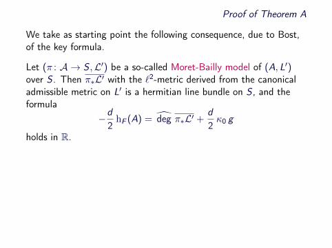
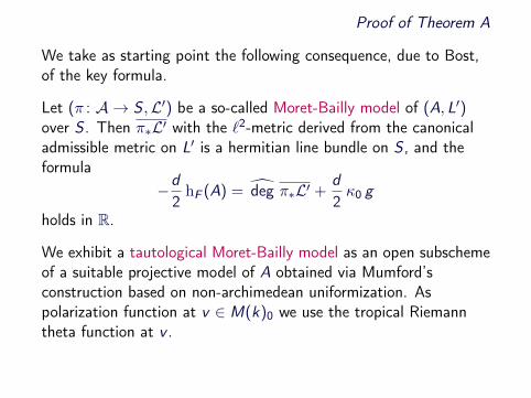
We take as starting point the following consequence, due to Bost,of the key formula.
Let (π : A → S ,L′) be a so-called Moret-Bailly model of (A, L′)over S . Then π∗L′ with the `2-metric derived from the canonicaladmissible metric on L′ is a hermitian line bundle on S , and theformula
−d
2hF (A) = deg π∗L′ +
d
2κ0 g
holds in R.
We exhibit a tautological Moret-Bailly model as an open subschemeof a suitable projective model of A obtained via Mumford’sconstruction based on non-archimedean uniformization. Aspolarization function at v ∈ M(k)0 we use the tropical Riemanntheta function at v .
For the tautological Moret-Bailly model we calculate deg π∗L′explicitly.
Proof of Theorem A
We take as starting point the following consequence, due to Bost,of the key formula.
Let (π : A → S ,L′) be a so-called Moret-Bailly model of (A, L′)over S . Then π∗L′ with the `2-metric derived from the canonicaladmissible metric on L′ is a hermitian line bundle on S , and theformula
−d
2hF (A) = deg π∗L′ +
d
2κ0 g
holds in R.
We exhibit a tautological Moret-Bailly model as an open subschemeof a suitable projective model of A obtained via Mumford’sconstruction based on non-archimedean uniformization. Aspolarization function at v ∈ M(k)0 we use the tropical Riemanntheta function at v .
For the tautological Moret-Bailly model we calculate deg π∗L′explicitly.

Proof of Theorem A
We take as starting point the following consequence, due to Bost,of the key formula.
Let (π : A → S ,L′) be a so-called Moret-Bailly model of (A, L′)over S . Then π∗L′ with the `2-metric derived from the canonicaladmissible metric on L′ is a hermitian line bundle on S , and theformula
−d
2hF (A) = deg π∗L′ +
d
2κ0 g
holds in R.
We exhibit a tautological Moret-Bailly model as an open subschemeof a suitable projective model of A obtained via Mumford’sconstruction based on non-archimedean uniformization.
Aspolarization function at v ∈ M(k)0 we use the tropical Riemanntheta function at v .
For the tautological Moret-Bailly model we calculate deg π∗L′explicitly.
Proof of Theorem A
We take as starting point the following consequence, due to Bost,of the key formula.
Let (π : A → S ,L′) be a so-called Moret-Bailly model of (A, L′)over S . Then π∗L′ with the `2-metric derived from the canonicaladmissible metric on L′ is a hermitian line bundle on S , and theformula
−d
2hF (A) = deg π∗L′ +
d
2κ0 g
holds in R.
We exhibit a tautological Moret-Bailly model as an open subschemeof a suitable projective model of A obtained via Mumford’sconstruction based on non-archimedean uniformization. Aspolarization function at v ∈ M(k)0 we use the tropical Riemanntheta function at v .
For the tautological Moret-Bailly model we calculate deg π∗L′explicitly.

Proof of Theorem A
We take as starting point the following consequence, due to Bost,of the key formula.
Let (π : A → S ,L′) be a so-called Moret-Bailly model of (A, L′)over S . Then π∗L′ with the `2-metric derived from the canonicaladmissible metric on L′ is a hermitian line bundle on S , and theformula
−d
2hF (A) = deg π∗L′ +
d
2κ0 g
holds in R.
We exhibit a tautological Moret-Bailly model as an open subschemeof a suitable projective model of A obtained via Mumford’sconstruction based on non-archimedean uniformization. Aspolarization function at v ∈ M(k)0 we use the tropical Riemanntheta function at v .
For the tautological Moret-Bailly model we calculate deg π∗L′explicitly.


![arXiv:math/0301201v3 [math.NT] 28 Jul 2004 Gerd Faltings, Michael Harris, Luc Illusie, Fumiharu Kato, Kazuya Kato, Minhyong Kim, Barry Mazur, Yoichi Mieda, Yukiyoshi Nakkajima, Richard](https://static.fdocuments.us/doc/165x107/5b8aa0a47f8b9af94b8c95d2/arxivmath0301201v3-mathnt-28-jul-2004-gerd-faltings-michael-harris-luc-illusie.jpg)


![Limited Discrepancy Search for flexible shop scheduling · Limited Discrepancy Search for flexible shop scheduling ... [Carlier & Néron, 2000]; [Lin & Liao, 2003] – Lower ... –](https://static.fdocuments.us/doc/165x107/5b0b1fbc7f8b9ac7678d9661/limited-discrepancy-search-for-flexible-shop-discrepancy-search-for-flexible-shop.jpg)

