Falling cat robot lands on its feet

Ben Shields, William S. P. Robertson, Natalie RedmondRoss Jobson, Rian Visser, Zebb Prime, Ben Cazzolato

School of Mechanical Engineering, The University of Adelaide, Australiabenjamin.shields@student.adelaide.edu.au will.robertson@adelaide.edu.au

Abstract

Cats are renowned for their ability to alwaysland on their feet. When their body is droppedwith no initial net angular momentum, they areable to rotate in the air using a variety of mech-anisms, including the use of a variable differ-ence between the moment of inertia of the frontand back portions of their body due to the mo-tion of their legs. The aim of this project is tobuild a robotic falling cat than can right itself inthe air not dissimilar in appearance and mech-anism to a biological cat. This paper describesthe first steps of creating a simplified modeland designing a simulation to demonstrate themechanism of a prototype. Theory is presentedto calculate input torques to achieve rotationfrom any drop angle or (sufficiently large) dropheight, and SimMechanics is used to verify andsimulate the model.

1 Introduction

The self-righting behaviour of a falling cat (and otheranimals) is well known, and there are a number of expla-nations on the mechanisms by which a falling cat rightsitself. Yeadon [1984] lists three mechanisms by whicha body composed of multiple links achieves changes oforientation in flight, using any combination of: (a) thevarying moments of inertia twist, (b) the two-axes twist,and/or (c) the ‘hula’ twist. Early consideration of afalling cat proposed the moments of inertia twist as themain mechanism [Benton, 1912], in which the extensionand retraction of the legs change the moments of inertiawhile the spine twists. This ‘legs-in-legs-out’ method isstill commonly used as an explanation of the problem to-day [Stewart, 2011]. However, it has recently been shownfor a reasonable model of such a system with typicalcat-like physical parameters that the maximum amountof rotation that can be achieved using this method isaround 55◦ [Kaufman, 2013].

Yeadon [1984], citing Batterman [1974], remarks thatthe cat uses a combination of the legs-in-legs-out twistand the ‘hula’ twist, in which the rear body and legscircumducts using spinal bending in an opposite sense tothe front body. As a point of difference, the self-rightingof a falling rabbit uses the two-axes twist, which requireslarge amounts of spinal twist [Yeadon, 1984] which is notobserved in a falling cat [Kane and Scher, 1969].

The first dynamic model to take into account the phys-iological constraints of the biological system was by Kaneand Scher [1969], who remarked that his model achievesverismilitude with a model of a cat ‘at the expense ofsimplicity’, although changes in moment of inertia dueto the varying positions of the legs are not considered.Kane’s model is notable in that the torso is constrainedto bending motion only, and cannot twist, and this hasbeen the basis for most simulated models since. Modernwork has largely focused on trajectory planning and op-timisation for falling cat models which use variations ofKane’s model [Weng and Nishimura, 2002; Ge and Chen,2007; Iwai and Matsunaka, 2012; Takahashi, 2012], butthe most complex simulation model proposed to date isa biomechanical model with 16 degrees of freedom and10 joint torque inputs [Arabyan and Tsai, 1998].

Despite the development of a number of simulatedmodels of varying complexity, no robotic systems in theliterature have been built to specifically implement someor all of the mechanisms of a self-righting falling cat.Maintaining a cat-like design and motion and producinga working physical model will distinguish this projectfrom prior work. The motivation to do so is to explorethe possibility of incorporating such behaviour into arobotic system, and determine whether a simplified ver-sion of this motion can achieve successful results.

The aim of this paper is to present a mechanically-simple model of a falling cat which is being developedinto a physical prototype. The prototype is under con-struction and its details will be reported at a future date.

This paper is structured into the following sections:the simplified cat model is presented, followed by the

Proceedings of Australasian Conference on Robotics and Automation, 2-4 Dec 2013, University of New South Wales, Sydney Australia

(a) Cat initially upside-down. (b) Front legs retracted to increasepositive rotation of front; back legsextended to reduce negative rota-tion of rear.

(c) Holds position and both halvescontinue to rotate.

(d) Front legs extended to reducenegative rotation; back legs retractto increase positive rotation.

(e) Holds position until required ro-tation is achieved.

(f) Back legs are now extended andbraced for impact.

Figure 1: Drawings of a falling cat denoting key points in the trajectory. Inspired by high speed footage [Destin, 2012].

derivation of a rigid-body dynamic model of the systemthat takes into account variable moments of inertia. Thisis followed by an analysis of the timing stages requiredto active the desired action of righting the cat duringits fall. Finally, a SimMechanics model is presented totest the theory, and the paper concludes with a briefdiscussion of the robotic system under development.

2 Simplified cat model

For the purposes of a robotic system a number of sim-plifications were required to reduce the complexity ofthe mechanical design from that of a biological feline.A physical cat uses a combination of spine flexion, per-haps some spinal twist, and leg extension to manipulateits moments of inertia, as discussed in the introduction.The aim of the project is to build a robotic cat, yet thecomplexity of the biological system precludes a simplemechanical design (cf. the comments of Kane and Scher[1969] on simplicity quoted prior). For the first itera-tion of the project, therefore, a radical simplification ismade to only model the legs-in-legs-out behaviour of acat since it has the easiest mechanical design. Whilethe work of Kaufman [2013] suggests this approach isimpossible, another alteration is made to the cat design

to allow a full 180◦ rotation to be achieved. Instead oflegs which extend out from the body all with approxi-mately equal density, ‘feet’ are added which act as largepoint masses to increase the possible change of momentof inertia.

The robotic cat model therefore consists of a body intwo halves that can rotate around their common axis (a‘rigid spine’), and each body has an attached leg that canextend to 90◦ and retract as needed. A schematic of thecat robot is shown in Figure 2. The axis of the spine waslocated roughly through the centre of the robot to sim-plify the calculation of the dynamics. Three actuatorsare required in total to control relative angle betweenthe front and back body halves and between each set oflegs and the body. Finally, note that for simplificationof the analysis the head is omitted.

3 Modelling of system dynamics

In the previous section the mechanism by which a fallingcat rights itself was presented. This section develops amodel by which this action can be emulated. With ref-erence to Figure 2, Table 1 defines the variables usedin the following sections. The values given for the vari-ables are indicative of the robotic system currently under

Proceedings of Australasian Conference on Robotics and Automation, 2-4 Dec 2013, University of New South Wales, Sydney Australia

FRONTBACK

m1m2

m3

m4

L1L2

2r

L

W2

W

θFθB

z

y

(a) Side view.

r

W2

L

W

2r

O

r4r3

r

x

y

(b) Front view.

Figure 2: Schematic and geometry of the robotic cat model.

Table 1: Variables used in modelling the robotic falling cat. Values shown are indicative and may be varied to suit.

Symbol Value Description

m1 2.75 kg Mass of front bodym2 1.95 kg Mass of back bodym3 0.4 kg Combined point mass of feetm4 0.074 kg Combined mass of legsL 13 mm Length of the legsW 3 mm Width of the legs2r 13 mm Width and height of the bodyθF , θB 0◦ to 90◦ Angle of the legs from the vertical (legs retracted for θ = 0◦)IOF 0.007 kg m2 Moment of inertia of front bodyIOB 0.005 kg m2 Moment of inertia of back bodyIF 0.016 kg m2 to 0.0477 kg m2 Moment of inertia of front body with legs and feet from θ = 0◦ to 90◦

IB 0.014 kg m2 to 0.0456 kg m2 Moment of inertia of back body with legs and feet from θ = 0◦ to 90◦

Proceedings of Australasian Conference on Robotics and Automation, 2-4 Dec 2013, University of New South Wales, Sydney Australia

construction; this section introduces a method by whichthese values can be chosen to fulfil a certain design cri-teria.

3.1 Conservation of angular momentumand theory of rotation

It can be considered that a cat separates its body intotwo separate rotational axes for the front and back por-tions of its body. Assuming that the cat falls from rest,the initial net angular momentum is zero and the sum ofthe angular momenta must also equal zero due to con-servation of momentum. This is represented as

IFωF + IBωB = 0, (1)

where IF and IB are the moments of inertia of the frontand back halves, respectively, and ωF and ωB are thecorresponding angular velocities. Therefore in order tocontrol the individual rotations of the front and backhalves of the cat, their respective angular velocities canbe controlled by adjusting the ratio of moments of iner-tia, IF /IB and IB/IF :

ωB = −IFIBωF , ωF = −IB

IFωB . (2)

Considering this in terms of a cat’s body, extending thelegs (increasing θ to 90◦) increases the moment of iner-tia and reduces angular velocity, while retracting the legs(decreasing θ) decreases moment of inertia and increasesangular velocity. When a cat is falling, it retracts itsfront legs (θ = 0◦) and rotates quickly clockwise, whilethe back legs remain extended (θ = 90◦) and rotateslowly anticlockwise, due to the conservation of angu-lar momentum. The cat then reverses the position of itslegs by extending its front legs and rotates slowly anti-clockwise and retracts its back legs and rotates quicklyclockwise. This motion is shown in Figure 1.

3.2 Moments of inertia

The cross-section of the cat’s body is comprised of arectangle and a semi-circle, as shown in Figure 2. Someassumptions where made in developing the inertia modelof the system. The front and back bodies are assumedto rotate about point O shown in the figure. (For therobotic system under development, this can be adjustedsomewhat using additional weights.) The pairs of legson each half are assumed to move as one, which alsosimplifies mechanical design as a single actuator can beused for each leg pair. The legs are designed to have lowmass and therefore low moment of inertia, and the feetare designed to have high mass and a correspondinglyhigh moment of inertia when the legs are fully extendedto 90◦. The feet are assumed to be point masses atthe end of the legs, which are modelled as slender rods.

Finally, the central shaft around which the bodies rotateis assumed to have negligible moment of inertia.

The total moments of inertia around the z axis of thefront and back body are given by, respectively,

IF = IOF + ILF + IFF , (3)

IB = IOB + ILB + IFB . (4)

where IOF , IOB are the moments of inertia due to thebodies, ILF , ILB due to legs, and IFF , IFB due to thefeet.

The front and back bodies each respectively have aconstant moment of inertia around the z axis given by

IOF = 12Cm1r

2 + 23Sm1r

2, (5)

IOB = 12Cm2r

2 + 23Sm2r

2, (6)

where S and C are the cross-sectional area ratios of thebody from the rectangle and the semi-circle respectively:

S =Arect

Arect +Acirc=

2r2

2r2 + πr2/2=

4

4 + π, (7)

andC = 1 − S =

π

4 + π. (8)

The front and back feet are assumed to be point masseswith moments of inertia, respectively,

IFF = m3r23, IFB = m3r

23. (9)

Finally, the moments of inertia due to the front and backlegs (without feet) are given by, respectively,

ILF =m4L

2θ

12+m4r

24, ITB =

m4L2θ

12+m4r

24, (10)

where Lθ is the projection of the leg length in the x–yplane, including the square top face of width W ,

Lθ = (L−W ) sin θ +W. (11)

and distance magnitudes of the feet and legs, r3 and r4,are

rx = r − 12W, ry = r + 1

2W, (12)

r23 = r2x + (ry + L sin θ)2, (13)

r24 = r2x +(ry + 1

2L sin θ)2. (14)

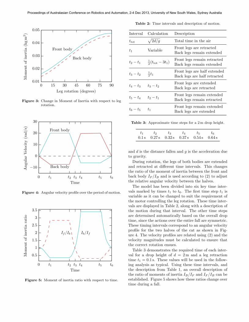
Figure 3 demonstrates the change in the moment ofinertia of each body due to rotation of the legs.

3.3 Angular velocity requirements

The overall fall time ttot can be calculated usingparabolic equations of motion, where

ttot =√

2d/g, (15)

Proceedings of Australasian Conference on Robotics and Automation, 2-4 Dec 2013, University of New South Wales, Sydney Australia

Back body

Front body

Mom

entof

inertia(kgm

2)

Leg rotation (degrees)

0 15 30 45 60 75 900.01

0.02

0.03

0.04

0.05

Figure 3: Change in Moment of Inertia with respect to legrotation.

Back body

Front body

Angu

larVelocity

(rad

/s)

Time

0 t1 t2 t3 t4 t5 t6

−10

0

10

20

30

Figure 4: Angular velocity profile over the period of motion.

Ib/IfIf/Ib

Mom

entof

inertiaratio

Time

0 t1 t2 t3 t4 t5 t6

0.5

1

1.5

2

2.5

3

3.5

Figure 5: Moment of inertia ratio with respect to time.

Table 2: Time intervals and description of motion.

Interval Calculation Description

ttot√

2d/g Total time in the air

t1 VariableFront legs are retractedBack legs remain extended

t2 − t112 (ttot − 3t1)

Front legs remain retractedBack legs remain extended

t3 − t212 t1

Front legs are half extendedBack legs are half retracted

t4 − t3 t3 − t2Front legs are extendedBack legs are retracted

t5 − t4 t2 − t1Front legs remain extendedBack legs remain retracted

t6 − t5 t1Front legs remain extendedBack legs are extended

Table 3: Approximate time steps for a 2 m drop height.

t1 t2 t3 t4 t5 t60.1 s 0.27 s 0.32 s 0.37 s 0.54 s 0.64 s

and d is the distance fallen and g is the acceleration dueto gravity.

During rotation, the legs of both bodies are extendedand retracted at different time intervals. This changesthe ratio of the moment of inertia between the front andback body IF /IB and is used according to (2) to adjustthe relative angular velocity between the halves.

The model has been divided into six key time inter-vals marked by times t1 to t6. The first time step t1 isvariable as it can be changed to suit the requirement ofthe motor controlling the leg rotation. These time inter-vals are displayed in Table 2, along with a description ofthe motion during that interval. The other time stepsare determined automatically based on the overall droptime, since the actions over the entire fall are symmetric.These timing intervals correspond to an angular velocityprofile for the two halves of the cat as shown in Fig-ure 4. The velocity profiles are related using (2) and thevelocity magnitudes must be calculated to ensure thatthe correct rotation ensues.

Table 3 demonstrates the required time of each inter-val for a drop height of d = 2 m and a leg retractiontime t1 = 0.1 s. These values will be used in the follow-ing analysis as typical. Using these time intervals, andthe description from Table 1, an overall description ofthe ratio of moments of inertia IB/IF and IF /IB can beestablished. Figure 5 shows how these ratios change overtime during a fall.

Proceedings of Australasian Conference on Robotics and Automation, 2-4 Dec 2013, University of New South Wales, Sydney Australia

Table 4: Moment of inertia ratio for each time interval.

Time Interval Ratio

t1 γ1 = IF,45◦/IB,90◦t2 − t1 γ2 = IF,0◦/IB,90◦t3 − t2 γ3 = IF,22.5◦/IB,67.5◦t4 − t3 γ4 = IB,25.5◦/IF,67.5◦t5 − t4 γ5 = IB,0◦/IF,90◦t6 − t5 γ6 = IB,45◦/IF,90◦

Given a series of time periods and ratios of momentof inertia as a function of time, it is now possible tocalculate the necessary angular velocities to achieve thedesired rotation. These calculations are simplified byassuming a piece-wise model for the moment of inertiaratios by taking an average of the moment of inertiaover each time interval. These averages are displayed inTable 4.

It can be seen in Table 4 that for half the time the ratiois defined as IF /IB and for the other half it is the inverseIB/IF . This is because the model has been constructedsuch that each body will ‘control’ the rotation for half ofthe fall time, using the calculations of angular velocityin (2), where ωB is ‘controlled’ in the first half and ωFis controlled in the second.

From this, simultaneous equations can be constructedrepresenting the motion of each body during the overallfall time. We can equate the overall rotation to an angleφ, which is the required angle of rotation to reach anupright position, resulting in

φ = ω1c1 − ω2c2, (16)

φ = −ω1c3 + ω2c4, (17)

where ω1 and ω2 are the peak angular velocities in rad/sfor the front and back body respectively, and time con-stants c(·) are given by

c1 =t12

+ (t2 − t1) +t3 − t2

2,

c2 =t4 − t3

3γ4 + γ5(t5 − t4) +

t6 − t53

γ6,

c3 =t13γ1 + γ2(t2 − t1) +

t3 − t23

γ3,

c4 =t4 − t3

2+ (t5 − t4) +

t6 − t52

.

(18)

These time constants are chosen heuristically becausethe moments of inertia change with angle, based on cor-rections to the areas under the velocity curves. As willbe seen in the simulation results in the next section (Fig-ure 9), the resultant velocity profile is reasonably closeto that desired.

Back legs

Front legs

Back body

Front body

Angu

larVelocity

(rad

/s)

Time

0 t1 t2 t3 t4 t5 t6−40

−20

0

20

40

Figure 6: Angular velocity profile over the period of motion.

Eqs 16 and 17 can be expressed in matrix form as[c1 −c2−c3 c4

] [ω1

ω2

]=

[φφ

], (19)

and the required angular velocities can be found with[ω1

ω2

]=

[c1 −c2−c3 c4

]−1 [φφ

]. (20)

The time constant matrix is invertible provided the timesteps and moment of inertia ratios are not chosen degen-erately.

The angular velocity of the legs can be considered sep-arately from the main body. When the legs are extendedor retracted it is required that they rotate 90◦ in t1 sec-onds. Using an example value of 0.1 s for t1, the requiredaverage velocity of the legs is 15.7 rad/s. The velocityprofile of the legs in conjunction with the body veloci-ties is shown in Figure 6.

Having calculated desired (and approximate) velocityprofiles for the robot, in the next section a dynamic sim-ulation is presented to verify that the motion of the robotis as expected.

4 SimMechanics model

SimMechanics is a multi-body simulation environmentfor 3D mechanical systems. The systems are modelledusing blocks representing bodies, joints, constraints,and force elements. SimMechanics then formulates andsolves the equations of motion for the complete dynamicsystem. The model can be parameterised using variablesand expressions defined within Matlab and the controlsystem for the bodies can be defined within Simulink.The purpose of SimMechanics is to verify the model cal-culations and provide a simulation of the expected sys-tem dynamics.

Proceedings of Australasian Conference on Robotics and Automation, 2-4 Dec 2013, University of New South Wales, Sydney Australia

The body of the cat has two separate rotational axisfor the front and back parts of its body. The simulationenvironment does not account for the conservation of an-gular momentum for the body as a whole, and thereforethe front and back body have to be analysed separately.

Before a dynamic analysis can be undertaken, the ge-ometry and material for the system needed to be estab-lished. This was achieved by using blocks for the bodies,joints and constraints, and applying the required speci-fications. SimMechanics is linked to the code developedfor the conceptual design, so if changes are made to thedesign, it can directly updated to the model. The blockswere defined to have a uniform density, which was estab-lished from the required mass and shape geometry. Uni-form density is a simplification on the real model, as itwill have localised mass from internal components. Sim-Mechanics then applies this density in accordance withthe geometry of the SimMechanics model to determinethe overall mass moment of inertia of each element.

4.1 Torque inputs

In Section 3, a model was presented that could achievethe desired rotational behaviour following a set of angu-lar velocity profiles. For the SimMechanics and roboticmodel, the inputs into the system are motor torques. Forsimplicity an open loop control methodology was chosen,such that torque profiles would be selected to achieveknown velocity profiles.

It was expected that knowing the angular velocity re-quirements, the appropriate acceleration and thereforetorque could be determine for each time interval of themotion. However, while the legs are extending or re-tracting the moment of inertia is changing as a func-tion of time. If the torque is set at a constant level,the imposed acceleration will therefore change due to itsinversely proportional relationship with the moment ofinertia. This is not ideal as the velocity profiles wereinitially set up assuming a constant acceleration; this isalso the reason heuristic time constants were required inEquation 18. To overcome this issue, each time inter-val was divided into smaller increments, and the torquein each increment was estimated to approximate the de-sired acceleration profile. Using the results of Figure 3,an approximation for the moment of inertia could be es-tablished, and the torque would be re-set to correlatewith the required angular acceleration.

In addition to the variable torque required to achievethe angular velocity profiles, there is an additional torquerequired to hold the legs in position due to the cen-tripetal force caused by rotation of the body. Duringintervals where the body is accelerating, the magnitudeof this centripetal force varies with time. Again, to ac-count for this variable torque requirement the velocityprofile was broken down into smaller time increments to

Body

Back legsFront legs

Torque(N

m)

Time

0 t1 t2 t3 t4 t5 t6−15

−10

−5

0

5

10

15

Figure 7: Torque inputs into the legs and body, discretisedevery 25 ms and 10 ms respectively, to achieve theresults shown in Figure 9.

give a more accurate approximation of the centripetalforce in order to be accounted for in the motor selectionfor the physical robot.

4.2 Simulation results

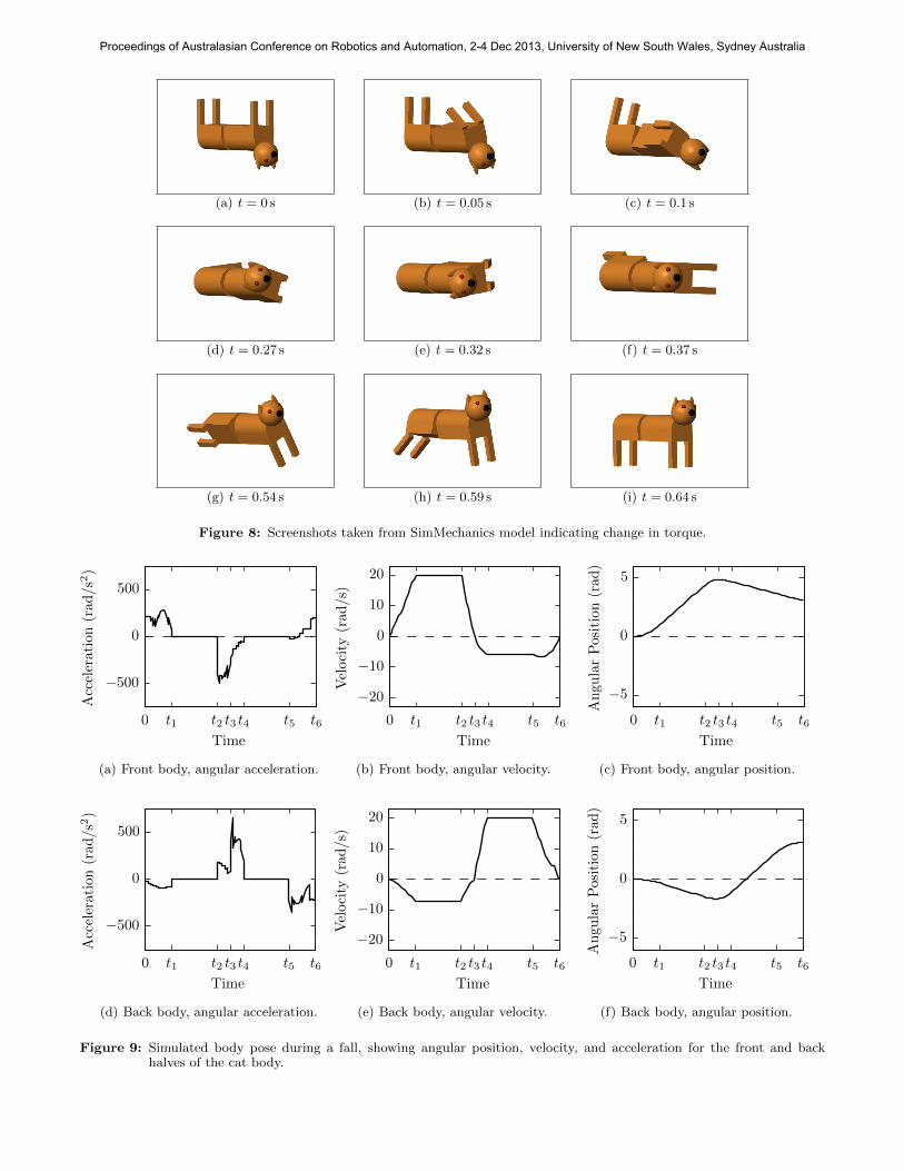
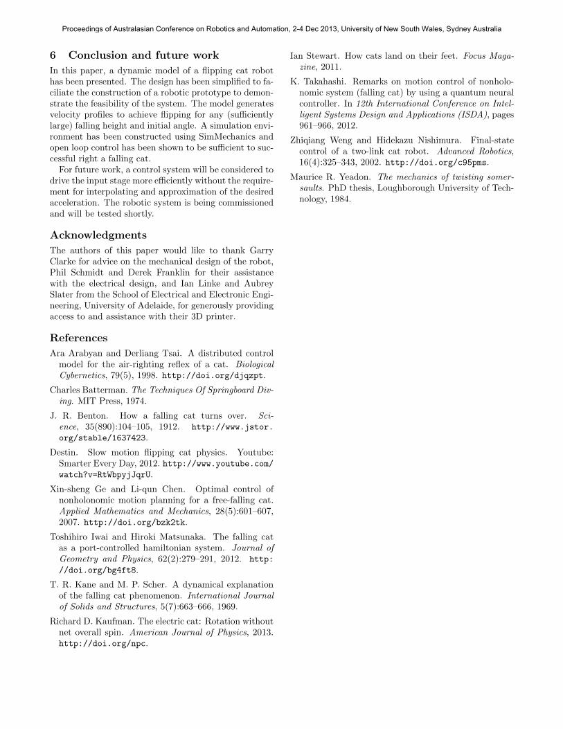
Starting from a set of system variables (masses, lengths,etc.), the velocity profiles were generated to achieve thedesired rotational action. These were taken as inputsinto the SimMechanics model, which in turn generatedstep-wise torque inputs, shown in Figures 7, to approx-iate these velocity profiles. The visual representation ofthe SimMechanics model can be seen in Figure 8, withassociated kinematic profiles as shown in Figure 9. Itcan be seen that although the stepwise approximationfor the input torques yields a noisy acceleration signal,the velocities track with the desired profile described inSection 3. These results demonstrate the consequence ofchoosing the legs-in-legs-out model for flipping: the rel-ative rotation between the front and back halves exceedsthat possible with a real cat.

5 Physical prototype

The simulation results presented in the previous sec-tion allowed design speculation for the specifications ofthe robotic system. An iterative process was conductedconsidering torque and weight requirements. (Largerweights required larger torques, which required largermotors, which increased the weight, etc.) It shouldbe noted that the technique used to generate the ac-celeration curves is not applicable to the DC motorsthat have been chosen, since their controllers allow a di-rect displacement input. This fact simplifies the controlmethodology of the robot significantly.

Proceedings of Australasian Conference on Robotics and Automation, 2-4 Dec 2013, University of New South Wales, Sydney Australia

(a) t = 0 s (b) t = 0.05 s (c) t = 0.1 s

(d) t = 0.27 s (e) t = 0.32 s (f) t = 0.37 s

(g) t = 0.54 s (h) t = 0.59 s (i) t = 0.64 s

Figure 8: Screenshots taken from SimMechanics model indicating change in torque.

Acceleration(rad

/s2)

Time

0 t1 t2 t3 t4 t5 t6

−500

0

500

(a) Front body, angular acceleration.

Velocity

(rad

/s)

Time

0 t1 t2 t3 t4 t5 t6

−20

−10

0

10

20

(b) Front body, angular velocity.

Angu

larPosition(rad

)

Time

0 t1 t2 t3 t4 t5 t6

−5

0

5

(c) Front body, angular position.

Acceleration(rad

/s2)

Time

0 t1 t2 t3 t4 t5 t6

−500

0

500

(d) Back body, angular acceleration.

Velocity

(rad

/s)

Time

0 t1 t2 t3 t4 t5 t6

−20

−10

0

10

20

(e) Back body, angular velocity.

Angu

larPosition(rad

)

Time

0 t1 t2 t3 t4 t5 t6

−5

0

5

(f) Back body, angular position.

Figure 9: Simulated body pose during a fall, showing angular position, velocity, and acceleration for the front and backhalves of the cat body.

Proceedings of Australasian Conference on Robotics and Automation, 2-4 Dec 2013, University of New South Wales, Sydney Australia

6 Conclusion and future work

In this paper, a dynamic model of a flipping cat robothas been presented. The design has been simplified to fa-ciliate the construction of a robotic prototype to demon-strate the feasibility of the system. The model generatesvelocity profiles to achieve flipping for any (sufficientlylarge) falling height and initial angle. A simulation envi-ronment has been constructed using SimMechanics andopen loop control has been shown to be sufficient to suc-cessful right a falling cat.

For future work, a control system will be considered todrive the input stage more efficiently without the require-ment for interpolating and approximation of the desiredacceleration. The robotic system is being commissionedand will be tested shortly.

Acknowledgments

The authors of this paper would like to thank GarryClarke for advice on the mechanical design of the robot,Phil Schmidt and Derek Franklin for their assistancewith the electrical design, and Ian Linke and AubreySlater from the School of Electrical and Electronic Engi-neering, University of Adelaide, for generously providingaccess to and assistance with their 3D printer.

References

Ara Arabyan and Derliang Tsai. A distributed controlmodel for the air-righting reflex of a cat. BiologicalCybernetics, 79(5), 1998. http://doi.org/djqzpt.

Charles Batterman. The Techniques Of Springboard Div-ing. MIT Press, 1974.

J. R. Benton. How a falling cat turns over. Sci-ence, 35(890):104–105, 1912. http://www.jstor.

org/stable/1637423.

Destin. Slow motion flipping cat physics. Youtube:Smarter Every Day, 2012. http://www.youtube.com/watch?v=RtWbpyjJqrU.

Xin-sheng Ge and Li-qun Chen. Optimal control ofnonholonomic motion planning for a free-falling cat.Applied Mathematics and Mechanics, 28(5):601–607,2007. http://doi.org/bzk2tk.

Toshihiro Iwai and Hiroki Matsunaka. The falling catas a port-controlled hamiltonian system. Journal ofGeometry and Physics, 62(2):279–291, 2012. http:

//doi.org/bg4ft8.

T. R. Kane and M. P. Scher. A dynamical explanationof the falling cat phenomenon. International Journalof Solids and Structures, 5(7):663–666, 1969.

Richard D. Kaufman. The electric cat: Rotation withoutnet overall spin. American Journal of Physics, 2013.http://doi.org/npc.

Ian Stewart. How cats land on their feet. Focus Maga-zine, 2011.

K. Takahashi. Remarks on motion control of nonholo-nomic system (falling cat) by using a quantum neuralcontroller. In 12th International Conference on Intel-ligent Systems Design and Applications (ISDA), pages961–966, 2012.

Zhiqiang Weng and Hidekazu Nishimura. Final-statecontrol of a two-link cat robot. Advanced Robotics,16(4):325–343, 2002. http://doi.org/c95pms.

Maurice R. Yeadon. The mechanics of twisting somer-saults. PhD thesis, Loughborough University of Tech-nology, 1984.

Proceedings of Australasian Conference on Robotics and Automation, 2-4 Dec 2013, University of New South Wales, Sydney Australia