Fair Operation of Multi-Server and Multi-Queue Systems

David RazSchool of Computer Science

Tel-Aviv University, Tel-Aviv, Israeldavidraz@post.tau.ac.il

Benjamin Avi-ItzhakRUTCOR, Rutgers University, New Brunswick, NJ, USA

aviitzha@rutcor.rutgers.edu

Hanoch LevySchool of Computer Science

Tel-Aviv University, Tel-Aviv, Israelhanoch@cs.tau.ac.il

November 3, 2004

Abstract

Multi-server and multi-queue architectures are common mechanisms used in a largevariety of applications (call centers, Web services, computer systems). One of the ma-jor motivations behind common queue operation strategies is to grant fair service tothe jobs (customers). Such systems have been thoroughly studied by Queueing Theoryfrom their performance (delay distribution) perspective. However, their fairness as-pects have hardly been studied and have not been quantified to date. In this work weuse the Resource Allocation Queueing Fairness Measure (RAQFM) to quantitativelyanalyze several multi-server systems and operational mechanisms. The results yieldthe relative fairness of the mechanisms as a function of the system configuration andparameters. Practitioners can use these results to quantitatively account for systemfairness and to weigh efficiency aspects versus fairness aspects in designing and con-trolling their queueing systems. In particular, we quantitatively demonstrate that: 1)Joining the shortest queue increases fairness, 2) A single “combined” queue system ismore fair than “separate” (multi) queue system and 3) Jockeying from the head of aqueue is more fair than jockeying from its tail.

1 Introduction

Multiple server queueing models have been used in a large variety of applications, including

computer systems, call centers and Web servers, as well as human waiting lines (e.g.,

in airports). The configuration and operation of multi-server (multi-processor) systems

involves a variety of operational mechanisms that must be chosen. These include the

1

number of queues and their dedication, the service policy, the queue joining policy and

queue jockeying rules.

An important motivation (perhaps the most important one) behind these mechanisms

is the wish to provide fair service to the jobs. Fairness in queues was stated to be an

important issue (for example [11, 10, 19, 17, 9]) and this importance (in the eyes of

customers) was reinforced by psychological experimental queueing studies [12, 13]. These

experimental studies have further shown that the single-queue system is perceived to be

more just (fair) compared to the multi-queue system.

Despite the importance of fairness, Queueing Theory, which devoted much effort to

the analysis of the above mentioned mechanisms, has dealt mainly with their performance

(in terms of delay and its moments) and the analysis of their relative fairness was not

carried out. The interest in computer job scheduling and in their fairness has recently

raised interest in quantitatively evaluating queue scheduling fairness. Work in this area

has been done in [4, 3, 6, 21, 16, 15, 2, 1, 14].

The purpose of this work is to use an analytic model, and evaluate the relative fairness

of multiple server systems. Such analysis will provide measures of fairness for these sys-

tems, that can be used to quantitatively account for fairness when considering alternative

designs. The quantitative approach can enhance existing design approaches in which usu-

ally efficiency (e.g., utilization and delays) is accounted for quantitatively, while fairness

is accounted for only in a qualitative way. Particular design issues that can be addressed

by this analysis include: 1) Whether to combine queues or not, 2) Whether to allow queue

jockeying, and 3) Queue joining policy.

To carry out this analysis we use the Resource Allocation Queueing Fairness Measure

(RAQFM) introduced in [16] for single server systems, and further researched in [15, 14].

This measure is based on the basic principle that all customers present at the system at

epoch t deserve equal service at that epoch, and deviations from that principle result in

discrimination (positive or negative); a summary statistics of these discriminations yields

a measure of unfairness. An important property of RAQFM is that it accounts for the

tradeoff between job seniority and job size (see [14]). As such it differs from alternative

queue fairness measures which were proposed in [1] and [21], which seem each to focus on

only one of these factors.

As mentioned above, RAQFM was first introduced in [16] for single server non-idling

systems. In that paper RAQFM was used to analyze and compare several service poli-

2

cies under the M/M/1 model. In [14] general properties of RAQFM were studied and a

methodology for analyzing RAQFM under any Markovian model was proposed. In [15]

RAQFM was generalized for non-idling multiple server systems and used in the context of

multiple classes and priorities. In [2] several job fairness measures, including RAQFM, are

compared to each other. In none of these papers were multiple server systems analyzed

thoroughly, especially the multiple queue case, which is the focus of this paper.

A detailed description of RAQFM, the model, and the notation are given in Section 2.

We start our analysis (Section 3) by considering G/D/m type systems, that is, systems

with a general arrival process and deterministic service times. Under this setting we first

show (Section 3.1) that Global FCFS1, namely serving the customers according to their

order of arrival, is the most fair service policy. This holds for any arrival process. This

property was proved in [14] for single server systems and is generalized here for multiple

server, multiple queue systems.

Second (Section 3.2), we study the effect of multiple queues on fairness. This is com-

monly referred to in the literature as the “Combining Queues” problem, in which a system

consisting of m M/M/1 queues, each having service rate µ and arrival rate λ (and denoted

the multi-queue system or the separate queue system) is compared to an M/M/m system

with the same service rate µ, and a corresponding arrival rate mλ (denoted the single

queue system or the combined queue system). It is widely known that the single queue

system is more efficient (a proof is given in [18]). However, if jockeying is allowed when a

server is idle (in a manner that is nondiscriminatory with respect to the required service

time), the systems have the same mean waiting time. In other cases, for example when

jockeying favors short jobs, the single queue system might even become less efficient than

the separate queue system (see [17] for a full discussion in the matter). As mentioned

above, in [12, 13] an experimental psychology study showed that a single queue system is

perceived to be more fair than a multiple queue one. Our goal is to quantitatively compare

the fairness of the combined queue G/D/m system to that of the separate queue G/D/m

system. We show that indeed the combined (single) queue system is more fair than the

separate (multiple) queue system.

Third, we investigate the jockeying-on-idle mechanism, namely jockeying is allowed

from a non-empty queue to an idle server, and conjecture that allowing for jockeying

increases the G/D/m system fairness. We show that jockeying from the head of the1In this entire paper, when we say FCFS we refer to Global FCFS, and similarly for LCFS

3

queue is more fair than jockeying from its tail (the latter practice is common in some

supermarkets).

Fourth, we study (Section 3.3) the effect of the queue joining policy on the fairness

of the system. Again, the efficiency aspect was thoroughly studied, starting with [22]

where the Shortest Queue (SQ) policy is shown to be optimal for exponential arrivals and

service times. Further work was done on extending the results for more general systems, for

example [5], where two identical exponential servers are considered (with similar results)

and [7] where a more general system is considered. Some cases where SQ is not optimal

are given in [20]. We study the fairness of the G/D/m system under SQ, Round-Robin

(RR), and Random Queue Joining (RAND). We show that SQ and RR are equivalent to

each other and they both are more fair than RAND.

Lastly for G/D/m type systems (3.4), we examine simulation results of these systems

under Poisson arrivals. The results support all the properties shown.

We then (Section 4) turn to study M/M/m type systems, namely systems with Poisson

arrivals and exponential service times. We provide an exact fairness analysis for the same

systems discussed in Section 3.2 and Section 3.3, for M/M/m type systems. The analysis of

each of these systems leads to a set of linear equations that needs to be solved numerically

to evaluate the fairness (unfairness) of the system. Numerical evaluation of these equations

(also supported by simulation) for a wide set of load parameters demonstrates that a)

the properties proved for the G/D/m type systems in Section 3.2 hold for M/M/m type

systems as well. b) the queue joining policy has little effect on the unfairness for M/M/m

type systems.

We then (Section 5) turn to examine G/G/m type systems. We show, via a simple

counter-case, that the results derived in Section 3 and Section 4 do not necessarily hold

for the G/G/m model. We nonetheless conjecture that some of the properties hold for the

G/GI/m model.

Lastly, concluding remarks are given in Section 6.

2 System Model and RAQFM

Consider a queueing system with m servers, indexed1, 2, . . . , m. All servers have equal

service rate, for simplicity a rate of one (unit of time per unit of time). The system is

subject to the arrival of a stream of customers, C1, C2, . . . , who arrive at the system at

4

this order. In order to focus on the effect multiple servers and multiple queues have on

the system fairness we assume all customers belong to the same class and have the same

priority.

Let al and dl denote the arrival and departure epochs of Cl respectively. Let sl denote

the service requirement (measured in time units) of Cl.

Corresponding to the way RAQFM was previously described in [16, 15, 14], the un-

fairness in the system is evaluated as follows: The basic fundamental assumption is that

at each epoch, all customers present in the system deserve an equal share of the service

given. If we let 0 ≤ ω(t) ≤ m denote the total service rate given at epoch t (which

usually is an integer equaling the number of working servers at that epoch), and N(t)

denote the number of customers in the system at epoch t, then the fair share, called the

momentary warranted service rate, is ω(t)/N(t). Let σl(t) be the momentary actual rate

at which service is given to Cl at epoch t. This is called the momentary granted ser-

vice rate. The momentary discrimination rate of Cl at epoch t, denoted δl(t), is therefore

δl(t) = σl(t)−ω(t)/N(t). This can be viewed as the rate at which customer discrimination

accumulates for Cl at epoch t. This is a generalization (proposed in [15]) of the definition

for the single server case, given in [16, 14].

The total discrimination of Cl, denoted Dl, is

Dl =∫ dl

al

δl(t)dt. (1)

Let D be a random variable denoting the discrimination of an arbitrary customer when

the system is in equilibrium. As shown in [15], the expected value of discrimination always

obeys E[D] = 0. Thus, according to RAQFM, the unfairness of the system is defined as

the second moment of the discrimination, namely E[D2], and denoted FD2 .

Throughout this paper we use ρ in its common definition as the system utilization

factor, which is ρdef= λx̄/m where λ is the average arrival rate and x̄ is the average service

time (e.g. [8, Sec. 2.1]).

Remark (Alternative Measure). Alternatively to setting ω(t) to be the amount of service

actually given at epoch t, one can set it to be the number of servers ω(t) = m or the number

of servers that can be utilized (depending on the number of customers present) ω(t) =

min(N(t),m). This will interpret an idle server as a source of negative discrimination

(which is not compensated by concurrent positive discrimination). We do not investigate

5

this measure here and it is the subject of future research.

3 Fairness of G/D/m Type Systems

In this section we analyze the fairness of G/D/m type systems, i.e. the customers ar-

rive according to a general arrival process, the service requirements of all customers are

identical, and the system has m servers.

3.1 The Effect of Seniority on Fairness

We start with analyzing the effect of customer seniority on fairness, and show that under

the G/D/m model serving customers in order of seniority increases system fairness.

Consider two customers Cj and Ck that are adjacently served, i.e. they are scheduled

to begin service adjacently, with arrival times aj < ak and equal service requirements,

i.e. sj = sk. Observe two possible cases: In the first case (Figure 1) they are served

sequentially, by the same server. In the second case (Figure 2) they are served by two

different servers in a partially-parallel manner.

We have two possible schedules: In schedule (a), (Figure 1(a), Figure 2(a)), the order

of seniority is preserved, i.e. Cj is served before Ck. In schedule (b), (Figure 1(b), Figure

2(b)), the order of service of Cj and Ck is interchanged and thus the order of seniority is

violated. We assume that both of the schedules are possible, i.e. that Cj and Ck reside in

the queue together for some time.

Service

��

��

Waiting

time

��

��

time

(a) Seniority Preserving Schedule

(b) Seniority Violating Schedule

Figure 1: Case 1 - Sequentially Served Customers (By The Same Server)

Lemma 3.1 (Preference of Seniority Between Adjacently Served Customers with Equal

Service Requirement). Let Cj and Ck be adjacently served customers, where aj < ak and

their service times are equal, i.e. sj = sk = s. Then the unfairness (measured as FD2)

6

Service

��

��

Waiting

time

��

��

(a) Seniority Preserving Schedule

(b) Seniority Violating Schedule

timeE1 E2 E3 E4 E5 E6

Figure 2: Case 2 - Partially Parallel Served Customers

of the seniority preserving schedule (a) is smaller than the unfairness of the seniority

violating schedule (b), for every arrival pattern.

Proof. We need to consider both cases. We note that the first case (Figure 1) is the only

case which was considered for single server systems in [14, Theorem 3.1], and it was proven

there that this lemma holds. We therefore only need to prove the second case (Figure 2).

Let Dai and Db

i denote the discrimination under schedule (a) and schedule (b) respec-

tively. Let F aD2 , F b

D2 denote the unfairness in the respective schedules, and let Na(t),

N b(t) denote the number of customers in the system at epoch t, respectively.

Let F̃ denote the total unfairness to all customers other than Cj and Ck, and let F̂

denote the total unfairness to Cj and Ck. Then FD2 = F̂ + F̃ .

Define ∆FD2 , ∆F̂ , and ∆F̃ to be the change, due to the interchange between Cj and

Ck, in the values of FD2 , F̂ , and F̃ respectively. We need to prove that ∆FD2 ≥ 0, where

∆FD2 = ∆F̂ + ∆F̃ =1L

[(Db

j)2 + (Db

k)2 − (Da

j )2 − (Dak)2

]

+1L

[ L∑

i 6=j,k

(Dbi )

2 −L∑

i6=j,k

(Dai )2

]. (2)

We divide the time interval (aj , max(dj , dk)) (namely from the arrival of Cj until both

Cj and Ck depart) into five sub-intervals, where interval i, i = 1, 2, 3, 4, 5, is (Ei, Ei+1),

and where E1 = aj ; E2 = ak; E3 is the first point in time where service to either Cj or Ck

starts; E4 is the point in time where service to the second customer starts; E5 = E3 + s;

E6 = E4 + s (see Figure 2).

7

We note that the number of customers in the system under schedule (a), Na(t), and

the number of customers in the system under schedule (b), N b(t), are identical for every

t. Therefore, the warranted service in interval i (of any customer) is the same in both

schedules, and we denote it R(i). As the warranted service in each interval is the same

in both schedules, and as other customers’ departure epochs are also the same in both

schedules, the interchange of Cj and Ck affects only Cj and Ck, i.e. Dai = Db

i , i 6= j, k.

Therefore ∆F̃ = 0, and from Eq.(2) it follows that

∆FD2 = ∆F̂ =1L

[(Db

j)2 + (Db

k)2 − (Da

j )2 − (Dak)2

]

=1L

[(s− (R(1) + R(2) + R(3) + R(4) + R(5))

)2

+(s− (R(2) + R(3) + R(4))

)2

− (s− (R(1) + R(2) + R(3) + R(4))

)2

− (s− (R(2) + R(3) + R(4) + R(5))

)2] =2L

R(1)R(5) > 0, (3)

where the inequality is due to R(i) > 0, i = 1, 2, 3, 4, 5.

Remark. Lemma 3.1 holds for sj = sk = s and regardless of the service times of the other

customers.

Define Φ to be the class of non-preemptive, non-divisible service polices (i.e. service

policies where once the server started serving a customer it will not stop doing so until

the customer’s service requirement is fulfilled, and at most one customer is served at any

epoch by each server), where the scheduler does not know the actual values of the service

times, or does not account for them in the scheduling decisions.

Theorem 3.1 (Fairness of FCFS and LCFS under G/D/m). If the service requirements of

all customers are identical, then for every arrival pattern, FCFS is the least unfair service

policy in Φ and LCFS is the most unfair one.

Proof. The proof is similar to the proof used in [14, Theorem 3.3] for single server systems.

Assume for the contradiction that there exists an arrival pattern and a service policy

φ ∈ Φ, φ 6= FCFS, which is the least unfair policy in Φ for this arrival pattern. Then the

8

order of service created by φ for this arrival pattern is different than the order of service

created by FCFS, otherwise φ is indistinguishable from FCFS.

Given this arrival pattern and the order of service created by φ, identify the first pair

of customers which are adjacently served and are not served according to their order of

arrival. Interchange the order of service between these two customers (which is certainly

possible). According to Lemma 3.1, the result of this interchange is a decrease in the

overall unfairness. Thus the resulting order of service is more fair than φ, in contradiction

to φ being the least unfair service policy for this arrival pattern.

A similar argument proves that LCFS is the most unfair policy in Φ.

3.2 The Effect of Multiple Queues Operation Mechanisms on Fairness

In this section we study several design and service decision considerations and examine

their effect on the system fairness.

The first practical issue is the use of multiple queues versus the use of a single queue

(also called sometimes ‘separate’ and ‘combined’ queues). In many cases both options are

physically possible, and the selection between them is done mainly based on the supposed

efficiency of the system (see [17]).

The second issue, assuming multiple queues are used, is jockeying. In some systems

jockeying is possible and we would like to find the effect it has on the system fairness. We

focus on jockeying done while a server is idle, in a manner that is nondiscriminatory with

respect to the required service time.

The third issue, assuming jockeying is possible, is whether jockeying should be done

from the head of the queue or from its tail. Note that from the efficiency (mean delay)

point of view there is no difference between the two manners, as long as the jockeying is

nondiscriminatory with respect to the required service time.

3.2.1 Multiple Queues Systems’ Description

For the sake of illustration, we analyze four systems. All four systems have m servers.

The first system has one common queue. A customer arriving at the system joins the tail

of the queue, and when a server becomes free it serves the customer at the head of the

queue, thus the system is non-idling2. The customers are therefore admitted into service2A system is non-idling if the number of busy servers (and thus the actual service rate) is always

min(N, m), where N is the number of customers in the system.

9

according to their order of arrival in a global FCFS manner. We refer to this system as

the single queue system.

The second system has m queues, where each of the servers serves only customers

joining its assigned queue, in a FCFS manner. Customers arriving at the system choose

one of the queues, or are assigned to one of the queues, and jockeying between the queues

is not permitted at any epoch. We refer to this system as the standard multiple queue

system. In this section we address a system where queue assignment (or joining) is done

randomly. In Section 3.3 we address the effect the queue joining policy has on the fairness.

The third and fourth systems have m dedicated FCFS queues, and jockeying is allowed

at epochs when a server is idle. When this happens, a customer from one of the non-

empty queues is immediately assigned to that server. Thus, as long as there are at least

m customers in the system, none of the servers is ever idle. We consider two manners

in which the jockeying customer is chosen, either from the head of one of the non-empty

queues or from the tail of one. We refer to the first as the head-jockeying-on-idle multi-

server system and to the second as the tail-jockeying-on-idle system. In both systems, if

there are several non-empty queues, then the queue from which the jockeying is done is

chosen randomly. For simplicity we do not address other manners in which that queue

can be decided.

As mentioned in Section 1, both jockeying-on-idle systems are known to be as efficient

as the single queue system, while the standard system is known to be less efficient than

the other three systems.

3.2.2 Multiple Queues Systems’ Properties

Theorem 3.2 (Single Queue is More Fair Than Multiple Queue for G/D/m). If the

service requirements of all customers are equal, then for every arrival pattern, the single

queue system has the lowest unfairness among the systems mentioned above.

Proof. The proof is immediate since serving in a single queue means serving in a global

FCFS manner, which is proven in Theorem 3.1 to be the most fair policy.

Theorem 3.3 (Head-Jockeying-On-Idle is More Fair Than Tail-Jockeying-On-Idle for

G/D/m). If service requirements of all customers are equal, and the choice of queue from

which jockeying is done is identical, then for every arrival pattern the head-jockeying-on-

idle system has lower unfairness than the tail-jockeying-on-idle system.

10

Proof. We prove that if the choice of queue from which jockeying is done is identical, the

policy with the lowest unfairness is one where jockeying is always done from the head of

the queue. Specifically, this proves that head-jockeying is more fair than tail-jockeying.

We prove this by way of contradiction. Assume for the contradiction that there exists

a jockeying policy ψ by which the jockeying customer is not always the customer at the

queue head, and that ψ is the policy with the lowest unfairness for every arrival pattern.

We will show that a policy with lower unfairness can be constructed.

Consider an arrival pattern where there exists an epoch e in which a server was idle,

and in which the customer admitted to the idle server by ψ was the n-th customer in

some non-empty queue, and n > 1. Say there are N customers in that queue, and denote

the customers in that queue C1, C2, . . . , CN , according to their order of arrival, with C1

being the first to arrive. We show that admitting Cn, n > 1 to the idle server has higher

unfairness than admitting Cn−1.

Say Cn was admitted to the idle server at epoch e, and Cn−1 was served at some later

epoch e′ > e. We construct a policy ψ′ that exactly imitates ψ, except it exchanges the

roles of Cn and Cn−1, i.e. Cn−1 is admitted at epoch e and Cn is served at epoch e′.

Since the customers are adjacent in the queue and have equal service requirements no

other customers are influenced by this exchange. Therefore, using the same notations and

arguments used in Lemma 3.1, ∆F = ∆F̂ and we need only to prove that ∆F̂ > 0. For

brevity and comparability with the proof of Lemma 3.1 we denote j = n− 1, k = n.

Let the service requirement of Cj and Ck be s. Two cases should be considered: either

e′−e < s or e′−e ≥ s. For e′−e < s observe that the situation is exactly the one depicted

in Figure 2, and as shown in the proof of Lemma 3.1 ∆F̂ > 0 in this case.

For the second case, e′ − e > τ , the situation is depicted in Figure 3. We divide the

Service

��

��

Waiting

��

��

time

(a) Seniority Preserving Schedule

(b) Seniority Violating Schedule

timeE1 E2 E3 E4 E5 E6

Figure 3: Selection of Jockeying Customer, Equal Service Requirements, Case 2.

11

time interval (aj , e′ + s) (namely from the arrival Cj until both Cj and Ck depart) into

five sub-intervals where interval i, i = 1, 2, 3, 4, 5, is (Ei, Ei+1), where E1 = aj ; E2 = ak;

E3 is the jockeying epoch e; E4 = E3 + s; E5 is the epoch where the second customer is

served, e′; E6 = E5 + s (see Figure 3).

Let the service warranted in interval i be R(i). Using Eq.(2) the difference in unfairness

is

∆F̂ =1L

[(s− (R(1) + R(2) + R(3) + R(4) + R(5))

)2

+(s− (R(2) + R(3))

)2

− (s− (R(1) + R(2) + R(3))

)2

− (s− (R(2) + R(3) + R(4) + R(5))

)2] =2L

R(1)(R(4) + R(5)) > 0. (4)

We therefore showed that for every service policy ψ that performs jockeying not always

from the head of the queue for at least one arrival pattern, a better policy ψ′ exists, in

contradiction to ψ being the policy with the lowest unfairness for every arrival pattern.

Therefore, the policy with the lowest unfairness for every arrival pattern must be one

where the jockeying customer is always the one at the queue head.

Remark. We have also shown that the worst policy is a policy in which the customer

admitted is always the one at the queue tail.

Conjecture 3.1 (Jocking-On-Idle is More Fair Than Standard Multi-Queue). If service

requirements of all customers are equal, then for every arrival pattern the standard system

is less fair than the jockeying-on-idle systems.

We base this conjecture on intuition.

Remark (Non-Equal Service Rate). As mentioned in Section 2 we limit our model to

servers with the same service rate (for simplicity a rate of one). It can be easily shown

that when this is not the case, the properties discussed above are not necessarily true. For

example, a more fair policy than FCFS might hold a senior customer in order to serve it

by a faster server.

12

3.3 The Effect of Queue Joining Policy on Fairness

In this section we address the effect of the queue joining on fairness. To this end we

analyze the head-jockeying-on-idle system with three queue joining policies: (a) customers

join queues at random (RAND) (b) customers always join the shortest queue (SQ), and

(c) customers join queues in a round-robin manner (RR).

Note that in practice selection of the the queue joining policy can be affected by several

physical factors of the system. These include who is making the queue joining decision

(the customer or a queue manager) and whether queue size information is available to the

decision maker.

Theorem 3.4 (Relative Fairness of Queue Joining Policies under the G/D/m Model). If

all service requirements are equal, then the unfairness in SQ equals that in RR, and both

have the lowest unfairness.

Proof. To prove that the unfairness for SQ equals that of RR note that if service require-

ments are equal, SQ and RR are in fact identical, since using round-robin always directs

a customer to the shortest queue.

Second, note that using SQ (or RR) yields an order of service which is in fact identical

to global FCFS, and from Theorem 3.1 Global FCFS is the most fair order of service.

3.4 Numerical Results for the M/D/2 Model

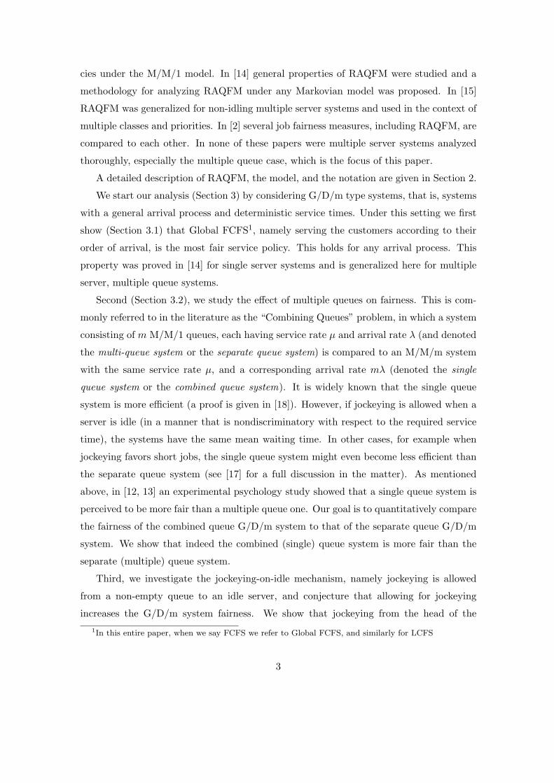
Figure 4 depicts numerical results from simulating the M/D/2 model as a function of

the system utilization factor ρ = sλ/2 for the four systems discussed in Section 3.2.1.

Service requirement was set as one unit (s = 1). Each point is the result of simulating

the passage of at least 106 customers through the system. The figure demonstrates the

following properties:

1. Except for one system and one point (single queue system at high load) the unfair-

ness is monotone increasing with the system utilization factor ρ. This monotonic behavior

was demonstrated several times before (see [16, 15, 14]). The reason for the decrease in

unfairness at high loads for the single queue system is still unclear and further study is

required.

2. The single queue system is more fair than all the multiple queue systems, for every

system load, as expected from Theorem 3.2. The ratio between the unfairness of the single

queue system and that of the head-jockeying-on-idle system increases with ρ, and reaches

13

0 0.2 0.4 0.6 0.8 10

0.05

0.1

0.15

0.2

0.25

ρ

E[D

2 ]

λ=ρ*2s=1

Standard Multi−QueueTail−Jockeying−On−IdlingHead−Jockying−On−IdlingSingle Queue

Figure 4: Unfairness of Four Queue Strategies under the M/D/2 Model

a ratio of more than 1 : 2 for ρ = 0.9. Recall that as long as jockeying is allowed only

in a manner that is nondiscriminatory with respect to the required service time (as is the

case with the multiple queue systems analyzed) the single queue system is also at least as

efficient as the multiple server systems.

3. Among the multiple queue systems, the jockeying-on-idle systems are more fair than

the standard (idling) system, for every system load. The ratio between the unfairness of the

standard system and that of the head-jockeying-on-idle system decreases with ρ, starting

with a high ratio of more than 1 : 8 for ρ = 1 and reaching a low of 1 : 1.9 for ρ = 0.9.

This agrees with Conjecture 3.1.

4. Among the jockeying-on-idle systems, head-jockeying is more fair than tail-jockeying

for every system load, as expected from Theorem 3.3. The difference between them in-

creases with ρ and is as high as 25% for ρ = 0.9. Recall that these two systems are equally

efficient.

In Figure 5 the three queue joining policies discussed in Section 3.3 are compared to

each other, as a function of the system utilization factor ρ, for the M/D/2 model. Service

requirement was set as one unit. Each point is the result of simulating the passage of at

least 106 customers through the system. The figure demonstrates the following properties:

1. SQ and RR are identical, as expected from Theorem 3.4. In fact, they are identical

to the single queue M/D/2 system.

2. RAND has higher unfairness than SQ and RR for every system load, as expected

from Theorem 3.4. The difference between them increases with ρ and is as high as 90%

for ρ = 0.9. Recall that these two systems are equally efficient.

14

0 0.2 0.4 0.6 0.8 10

0.02

0.04

0.06

0.08

0.1

0.12

0.14

ρ

E[D

2 ]

λ=ρ*2s=1

Join Random QueueJoin Round−RobinJoin Shortest Queue

Figure 5: Unfairness in the M/D/2 Model - Comparison of Queue Joining Policies

4 Fairness of M/M/m Type Systems

In this section we analyze the fairness of M/M/m type systems. We start with a description

of the assumptions and notations used in our analysis.

For the analysis in this section we will consider systems where the arrival of customers

follows a Poisson process with rate λ and the service requirements of the customers are

i.i.d. exponentially with mean 1/µ. Let ρdef= λ/µ be the fraction of busy servers (also

called the system utilization factor). For stability we assume ρ < 1.

Due to the Markovian nature of the system, and for mathematical convenience, time

can be viewed as being slotted where the sequence of arrivals and departures forms the

slot boundaries. Let Ti, i = 0, 1, . . . be the duration of the i-th slot.

We limit the analysis to systems where a service decision is made only on arrival and

departure epochs. Thus, the number of available servers, the number of servers actually

giving service, and the rate at which service is given to each customer, are constant during

each slot. We can therefore define 0 ≤ ωi ≤ m as the number of working servers in the i-th

slot, σi,l as the rate at which service is given to Cl at the i-th slot, and Ni as the number

of customers in the system during the i-th slot. δi,l, the momentary discrimination of Cl

during the i-th slot, which is the rate at which customer discrimination accumulates for

Cl at this slot, is δi,j = σi,l − ωi/Ni. The total discrimination accumulated for Cl during

the i-th slot is ci,lTi. Thus, the slotted version of Eq.(1) is Dl =∑yl

i=xlδi,lTi , where xl is

the index of the slot initiated by the arrival of Cl and yl is the index of the slot terminated

by the departure of dl.

15

4.1 The Effect of Multiple Queues on Fairness

In this section we provide quantitive fairness analysis, under the M/M/m model, for the

four systems described in Section 3.2.1, namely the single queue system, the standard

multiple queue system, and the two jockeying-on-idle systems - head-jockeying-on-idle

and tail-jockeying-on-idle. Recall that for all four systems the order of service whithin

each queue is FCFS, except for jockeying.

4.1.1 Fairness in Multiple Server Single Queue Systems under the M/M/m

Model

Consider a single queue system, as described in Section 3.2.1. Consider an arbitrary tagged

customer denoted C. Let a be the number of customers ahead of C in the queue, including

served customers. If C is in service, adef= 0. Let b be the number of customers behind C.

If C is in service, b includes also customers served by other servers. Note the (unavoidable)

jump occurring in the value of b when C enters service. Due to the Markovian nature of

the system, and due to non-idling, the state (a, b) captures all that is needed to predict

the future of C.

The momentary discrimination during a slot where C is in state (a, b), denoted δ(a, b),

is δ(a, b) = 1(a = 0) − s/(a + b + 1), where s is the number of customers served at that

state, s = min(m, a + b + 1), and 1(·) is the logical function (also called sometimes an

indicator function), i.e. 1(·) = 1 if the relation · is true and 1(·) = 0 otherwise.

We would like to compute E[D2], the unfairness of the system, as define in Section

2. Let E[D2|k] for k = 0, 1, . . . denote the expected value of the square of discrimina-

tion, given that the customer encounters k customers on arrival (including the ones being

served). Let pk be the steady state probability that there are k customers in the system.

According to the PASTA property (see [23]), this is also the probability that k customers

are seen by an arbitrary arrival. Thus, the second moment of D (the unfairness) follows

E[D2] =∞∑

k=0

E[D2|k]pk. (5)

16

The steady state probabilities for the single queue M/M/m system are:

pk

=

{p0

(mρ)k

k! k ≤ m

p0

ρkmm

m! k ≥ m

p0 =

[(mρ)m

m!(1− ρ)+

m−1∑

k=0

(mρ)k

k!

]−1, (6)

(e.g. [8, Sec. 3.5]).

In the case m = 2 these are equal to pk

= p02ρk k ≥ 1, p0 = (1 + ρ)/(1− ρ).

Let D(a, b) be a random variable denoting the discrimination experienced by a cus-

tomer, through a walk starting at (a, b), and ending at its departure. Then

E[D2|k] =

{E[D2(k, 0)] k ≥ m

E[D2(0, k)] k < m. (7)

Let d(a, b) and d(2)(a, b) be the first two moments of D(a, b).

In the single queue M/M/m system the slot lengths are exponentially distributed with

parameter λ + sµ and first two moments t(1)(a, b) = 1/(λ + sµ), t(2)(a, b) = 2(t(1))2 .

Define λ̃(a, b), the probability that the slot will end with a customer arrival event, and

µ̃(a, b), the probability that the slot will end with a customer departure from a specific

active server. Then λ̃(a, b) = λ/(λ + sµ), µ̃(a, b) = µ/(λ + sµ). Note that here and

throughout the paper λ̃ refers to the probability of an arrival of any customer, while µ̃

refers to the probability of a departure of a customer from one specific queue. This seeming

inconsistency is required for mathematical brevity.

Assume C is in state (a, b). At the slot’s end, the system will encounter one of the

following events and C’s state will change accordingly:

1. A customer arrives to the system. The probability of this event is λ̃(a, b). C’s state

changes to (a, b + 1).

2. For a > 0: A customer leaves the system. The probability of this event is sµ̃(a, b).

If a > m, C’s state changes to (a− 1, b). Otherwise, C’s state changes to (0, a + b− 1).

3. For a = 0, b > 0: A customer other than C leaves the system. The probability of

this event is (s− 1)µ̃(a, b). C’s state changes to (a, b− 1).

4. For a = 0: C leaves the system. The probability of this event is µ̃(a, b).

17

This leads to the following set of linear equations

d(a, b) = t(1)(a, b)δ(a, b) + λ̃(a, b)d(a, b + 1)

+ µ̃(a, b)

md(a− 1, b) a > m

md(0, a + b− 1) a = m

(s− 1)d(a, b− 1) a = 0, b > 0

(8)

d(2)(a, b) = t(2)(a, b)(δ(a, b))2 + λ̃(a, b)d(2)(a, b + 1)

+ µ̃(a, b)

md(2)(a− 1, b) a > m

md(2)(0, a + b− 1) a = m

(s− 1)d(2)(a, b− 1) a = 0, b > 0

+ 2t(1)(a, b)δ(a, b)

λ̃(a, b)d(a, b + 1)

+µ̃(a, b)

md(a− 1, b) a > m

md(0, a + b− 1) a = m

(s− 1)d(a, b− 1) a = 0, b > 0

. (9)

These sets of equations can be solved numerically to any required precision using simple

numeric methods. Solving these sets of equations yields d(2)(a, b), and substituting the

results in Eq.(7) yields E[D2|k]. Substituting these in Eq.(5) yields E[D2], the system

unfairness.

4.1.2 Fairness in Multiple Server Multiple Queue Systems

We now analyze the standard multiple queue system, as described in Section 3.2.1. Con-

sider an arbitrary tagged customer C. When C arrives into the system it joins a queue

at random. We refer to the queue that the customer joined as the local queue and to the

rest of the queues as the other queues. For the analysis we index the local queue 1, and

the other queues 2, . . . , m, in some arbitrary way.

Let a be the number of customers ahead of C in the local queue, including the served

customer, if such a customer exists. Let b be the number of customers behind C in the

local queue. Let li be the number of customers in the i-th queue, i = 2, . . . , m, including

18

any served customers, and let l denote the vector (l2, . . . , lm). Due to the Markovian

nature of the system, the state (a, b, l) captures all that is needed to predict the future of

C.

Define Σv, the sum of the elements of a vector v. Recall that s denotes the number

of active servers (the number of customers served). Since the server at the local queue is

active as long as C is in the system

s = 1 +∑

2≤i≤m

1(li > 0). (10)

The momentary discrimination during a slot in which C is in state (a, b, l), denoted

δ(a, b, l), is

δ(a, b, l) = 1(a = 0)− s

Σl + a + b + 1. (11)

Let k = k1, . . . , km denote a queue occupancy, where ki is the number of customers at

the i-th queue, including the customer in service. Let E[D2|k] denote the expected value

of the square of discrimination, given that the customer encounters occupancy k upon

arrival.

Let Pk be the steady state probability that the occupancy is k, Then

E[D2] =∞∑

k1=0

∞∑

k2=0

· · ·∞∑

km=0

E[D2|k]Pk. (12)

Note that the system consists of m independent M/M/1 queues, where each is utilized

a fraction ρ = λ/(µm) of the time and therefore Pk = (1− ρ)mρΣk .

Let D(a, b, l) be a random variable, denoting the discrimination experienced by a

customer, through a walk starting at (a, b, l), and ending at its departure. Let k̂i denote

the vector k, whose i-th element is ommited, i.e. k̂i = (k1, . . . , ki−1, ki+1, . . . , km). Using

this notation

E[D2|k] =1m

m∑

i=1

E[D2(ki, 0, k̂i)]. (13)

Let d(a, b, l) and d(2)(a, b, l) be the first two moments of D(a, b, l).

When C is in state (a, b, l) the slot length is exponentially distributed with parameter

λ + sµ and first two moments

t(1)(a, b, l) =1

λ + sµ, t(2)(a, b, l) = 2(t(1))2. (14)

19

Also define λ̃(a, b, l), the probability that the slot will end with a customer arrival and

µ̃(a, b, l), the probability that the slot will end with a customer departure event from a

specific active server. These are equal to

λ̃(a, b, l) =λ

λ + sµ, µ̃(a, b, l) =

µ

λ + sµ. (15)

Define Ii, the vector (l2 = 0, l3 = 0, . . . , li = 1, . . . , lm = 0).

At the slot end, the system will encounter one of the following events and C’s state

will change accordingly:

1. A customer arrives at the system, joining the i-th queue. The probability of this

event is λ̃(a, b, l)/m, for every value of i = 1, . . . , m, and the sum of these probabilities is

therefore λ̃(a, b, l). If i = 1, C’s state changes to (a, b+1, l). Otherwise, C’s state changes

to (a, b, l + Ii).

2. A customer leaves the system, from the i-th queue. This is possible only for

i = 2, . . . ,m such that li > 0, and for i = 1 (the local queue). The probability of

this event is µ̃(a, b, l), for each of the s non-empty queues, and the overall probability of

departure is therefore sµ̃(a, b, l). If i = 1 and a > 0, C’s state changes to (a − 1, b, l). If

i = 1 and a = 0 (C is being served), C leaves the system. If i > 1, C’s state changes to

(a, b, l− Ii).

This leads to the following set of linear equations

d(a, b, l) = t(1)(a, b, l)δ(a, b, l)

+ λ̃(a, b, l)1m

(d(a, b + 1, l) +

m∑

i=2

d(a, b, l + Ii))

+ µ̃(a, b, l)( ∑

2≤i≤m

1(li > 0)d(a, b, l− Ii)

+1(a > 0)d(a− 1, b, l)). (16)

A set of linear equations for d(2)(a, b, l) is brought in Appendix A Eq.(21).

Similarly to Section 4.1.1, solving these equation yields d(2)(a, b, l), substituting in

Eq.(13) yields E[D2|k], and substituting in Eq.(12) yields E[D2], the system unfairness.

20

4.1.3 Fairness in Multiple Server Multiple Queue Systems With Jockeying-

On-Idle

We now turn to the two jockeying-on-idle systems described in Section 3.2.1. First let

us define the jockeying-on-idle system behavior in more detail. When a customer arrives

to the system finding no idle servers, the customer is assigned to a queue randomly (we

discuss other options in Section 4.2). If at least one of the servers is idle, the customer is

assigned at random to one of the idle servers. In each queue the order of service is FCFS.

In the event that a server becomes idle a customer is assigned to that server from one of

the non-empty queues, where the queue is chosen randomly. In the head-jockeying-on-idle

system the assigned customer is the customer at the head of the chosen queue and in the

tail-jockeying-on-idle system the assigned customer is the customer at its tail.

The analysis of this system is almost identical to that of the standard system analyzed

in Section 4.1.2. The state definition is identical. s, the number of customers served, can

be calculated in a simpler way since s = min(Σl + 1,m), although Eq.(10) holds as well.

The momentary discrimination, the slot length moments, and the arrival and departure

probabilities follow Eq.(11), Eq.(14), and Eq.(15), respectively.

Note that due to non-idling some occupancy vectors are impossible, so Pk = 0 for

ki = 0, kj > 1, i, j = 1, . . . , m. For completeness in this case we also define E[D2|k]def= 0.

Using these definitions Eq.(12) holds, and the steady state probabilities can be numer-

ically calculated using the system’s balance equations, which we omit for brevity.

The relationship between E[D2|k] and D(a, b, l) is different in the jockeying-on-idle

systems, since the arriving customer is assigned to an idle server if such a server exists.

If Σk < m there are z = m − Σk idle servers and we let ei be the index of the i-th idle

server, i = 1, . . . , z. Then

E[D2|k] =

{1m

∑mi=1 E[D2(ki, 0, k̂i)] Σk ≥ m

1z

∑zi=1 E[D2(0, 0, k̂li)] Σk < m

. (17)

Let d(a, b, l) and d(2)(a, b, l) be the first two moments of D(a, b, l).

We can now enumerate the events possible at the end of every slot, which will yield

the desired sets of equations. Describing all the different possible events for the general

case is quite tedious, though possible. We therefore only describe them for the two servers

case, m = 2. In this case the state definition includes a, b, and l - the number of customers

in the other queue.

21

The possible events are:

1. A customer leaves the system from the local queue. The probability of this event is

µ̃(a, b, l). If a > 0 C’s state will change to (a− 1, b, l). Otherwise C leaves the system

2. For l = 0: A customer arrives at the system. The probability of this event is

λ̃(a, b, l). As l = 0, the customer will always choose the other queue, and thus C’s state

will change to (a, b, 1).

For l > 0 (3-5):

3. A customer arrives at the system, choosing the local queue. The probability of this

event is λ̃(a, b, l)/2, and C’s state will change to (a, b + 1, l).

4. A customer arrives at the system, choosing the other queue. The probability of this

event is λ̃(a, b, l)/2, and C’s state will change to (a, b, l + 1).

5. A customer leaves the system from the other queue. The probability of this event

is µ̃(a, b, l). If l > 1 C’s state will change to (a, b, l − 1). If l = 1 then at the end of this

slot a customer from the local queue will be served, as follows:

a) In the head-jockeying-on-idle system if a > 1 then C’s state will change to

(a− 1, b, 1), if a = 0, b > 0 then C’s state will change to (a, b − 1, 1), and if a, b = 0 then

C’s state will change to (0, 0, 0). If a = 1 then C will change queues, and thus C’s state

will change to (0, 0, b + 1).

b) In the tail-jockeying-on-idle system if b > 0 then C’s state will change to (a, b−1, 1), and again, if a, b = 0 then C’s state will change to (0, 0, 0). If a > 0, b = 0 then C

will change queues, and thus C’s state will change to (0, 0, a).

For head-jockeying-on-idle this leads to the following set of equations

d(a, b, l) = t(1)(a, b, l)δ(a, b, l)

+ λ̃(a, b, l)

{d(a, b, l + 1) l = 012

(d(a, b + 1, l) + d(b, b, l + 1)

)l > 0

+

µ̃(a, b, l)

d(a, b, l − 1) l > 1d(a− 1, b, l) l = 1, a > 1d(0, 0, b + 1) l = 1, a = 1d(a, b− 1, l) l = 1, a = 0, b > 0d(a, b, l − 1) l = 1, a = 0, b = 00 l = 0

22

+1(a > 0)d(a− 1, b, l)

). (18)

The set of equations derived for tail-jockeying-on-idle is brought in Appendix A Eq.(22).

Sets of linear equations for d(2)(a, b, l), similar to Eq.(9), are also derived, and we omit

them for brevity.

4.1.4 Numerical Results for the M/M/2 Model

We consider a system consisting of two servers. Figure 6 depicts the results from evaluating

the sets of equations provided in Section 4.1. The results are also supported by simulation.

For all plotted points µ = 1 while λ changes according to ρ. The figure demonstrates the

0 0.2 0.4 0.6 0.8 10

0.2

0.4

0.6

0.8

1

1.2

1.4

ρ

E[D

2 ]

λ=ρ*2µ=1

Standard Multi−QueueTail−Jockeying−On−IdlingHead−Jockying−On−IdlingSingle Queue

Figure 6: Unfairness of Four Queue Strategies for the M/M/2 Model

following properties:

1. For all systems, the unfairness is monotone increasing with the system utilization

factor ρ.

2. Similarly to the situation in the M/D/2 model, the single queue system is more

fair than all the multiple queue systems, for every system load. The difference in un-

fairness between this system and the best multiple server system, in our analysis the

head-jockeying-on-idle system, is around 10%. Recall that as long as jockeying is allowed

only in a manner that is nondiscriminatory with respect to the required service time (as

is the case in the systems analyzed) the single queue system is at least as efficient as the

multiple queue systems.

3. Similarly to the situation in the M/D/2 model, among the multiple queue systems,

the jockeying-on-idle systems are more fair than the idling system, for every system load.

23

The difference between these two types of systems is quite substantial. At lower loads,

the ratio between them can be more than 1:10.

4. Similarly to the situation in the M/D/2 model, among the jockeying-on-idle systems,

head-jockeying is more fair than tail-jockeying for every system load. The difference

between them is around 10%. Recall that these two systems are equally efficient.

To summarize, all three properties discussed in Section 3.2 for the G/D/m model (and

demonstrated to be true for the M/D/2 model in Section 3.4) are demonstrated to be true

for the M/M/2 model.

4.2 The Effect of Queue Joining Policy on Fairness

In this section we briefly analyze the queue joining policies discussed in Section 3.3, for

M/M/m type systems. The RAND policy was analyzed in Section 4.1.3, and thus we only

analyze the SQ and RR policies (with head-jockeying-on-idle). We only show the analysis

for the case of m = 2 (two servers and two queues).

4.2.1 Fairness in the Join The Shortest Queue Policy

The analysis of the SQ policy is almost identical to that of the RAND policy given in

Section 4.1.3.

One difference is that C always joins the shortest queue, and therefore Eq.(17) should

be corrected. A second difference is that in the event of a customer arrival the customer

always joins the shortest queue. Thus if l < a + b + 1 C’s state changes to (a, b, l + 1)

and if l > a + b + 1 C’s state changes to (a, b + 1, l). If l = a + b + 1 (the two queues are

of equal length), we assume the customer is assigned to one of the queues randomly, and

thus there is a λ̃(a, b, l)/2 probability of joining either of the queues. The set of equations

thus derived for d(a, b, l) is quite similar to Eq.(18): the first and third terms of the right

hand side of Eq.(18) remain the same, and the second term changes to

λ̃(a, b, l)

d(a, b, l + 1) l < a + b + 1d(a, b + 1, l) l > a + b + 112

(d(a, b + 1, l) + d(a, b, l + 1)

)l = a + b + 1

. (19)

Similarly, a set of linear equations for d(2)(a, b, l) is derived, which we omit for brevity.

24

4.2.2 Fairness in the Round-Robin Queue Joining Policy

Let r denote the index of the queue that the next arriving customer will join, r = 1, . . . , m.

The state (a, b, l, r) now captures all that is needed to predict the future of C. We use the

⊕ symbol to denote the modulo m addition, i.e. x⊕ ydef= (x + y) mod m.

The analysis is again nearly identical to that of the RAND policy given in Section 4.1.3,

except that r needs to be added to the state definition in every place it is used. Other

than that there are two other differences. First, Eq.(17) should be corrected to account

for C’s always joining the r-th queue. Second, other customers joining the system behave

accordingly. For m = 2, in the event of a customer arrival when r = 1 the customer joins

the local queue and thus C’s state changes to d(a, b+1, l, r⊕1). If r = 2 C’s state changes

to d(a, b, l + 1, r ⊕ 1). The set of equations derived is therefore quite similar to Eq.(18),

where the second term of the right hand side change to

λ̃(a, b, l)

{d(a, b + 1, l, r ⊕ 1) r = 1d(a, b, l + 1, r ⊕ 1) r = 2

. (20)

Similarly, a set of linear equations for d(2)(a, b, l) is derived, which we omit for brevity.

4.2.3 Numerical Results

Figure 7 depicts the unfairness of the three joining policies analyzed - random, round-

robin, and shortest queue, for the M/M/2 model, as a function of the system utilization

factor ρ. They were computed using the equations derived above. For comparison we also

plot the results for the single queue system and the results for the tail-jockeying-on-idle

system (with random queue joining). The results are also supported by simulation. The

figure demonstrates the following properties:

1. All three queue joining policies are less fair than the single queue system, and more

fair than the tail-jockeying system.

2. The unfairness of the system in the three queue joining policies is very similar. In

fact, the unfairness is within a 1% interval, which might be caused by inaccuracies in our

computation. This means that according to our analysis, in the case of head-jockeying-

on-idle M/M/2 systems, the queue joining policy (among the three policies studied) has

little effect on the fairness of the system.

25

0 0.2 0.4 0.6 0.8 10

0.1

0.2

0.3

0.4

0.5

0.6

0.7

0.8

ρ

E[D

2 ] λ=ρ*2µ=1

Tail−Jockeying−On−IdlingJoin Random QueueJoin Round−RobinJoin Shortest QueueSingle Queue

Figure 7: The Effect of the Queue Joining Policy on the System Fairness

Remark. The latter insensitivity to the queue joining policy can be explained by the

fact that the jockeying alleviates potential discrimination caused by unfair queue joining

policies.

5 Fairness of G/G/m Type Systems

In this section we consider type G/G/m systems, i.e. systems where the customers arrive

according to a general arrival process, the service requirements are generally distributed

and the system has multiple servers. We show, via a simple example, that results similar

to those derived in the analysis of the G/D/m system (Section 3.2) and demonstrated to

be true for M/M/m type systems (Section 4.1) do not necessarily hold for the G/G/m

system. Nonetheless the question whether these results hold for G/GI/m type systems

(namely where the service times are generally distributed and independent of each other

and of the arrivals), remains open and is left for future research.

In the following example we show that the single queue system is not necessarily more

fair than multiple queue systems with no jockeying. Consider the following two server sce-

nario, involving 4 customers, C1, C2, C3 and C4:{(ai, si)}i=1,2,3,4 = {(0, s+1), (0, 2ε), (ε, s+

1), (1, ε)}, where ε → 0 and s À ε is some finite service requirement. If customers are

served in a single queue, then C4, which has a very short service requirement, has to wait

s units of time to be served. As C2 is served immediately upon arrival and its service time

is very small, we can disregard this interval of service in our numerical calculation. This

leads to a relatively high unfairness, namely 2× (s× 1/3)2 + (s× (−2/3))2 = 2s2/3. Con-

sider now the two queues (qa and qb) case where jockeying is not allowed. Assume C1 joins

26

qa and C2 can join qb. C3 joins the system at epoch ε, finding both serves busy, and joins

qa (using round-robin joining policy, or randomly). C4 can then be served upon arrival. As

C2 and C4 are served immediately upon arrival and their service times are very small, we

can disregard these intervals of service in our numerical calculation. As C3 only needs to

wait for one customer, namely C1, compared to two customers for which C4 needs to wait

for in the previous case, the unfairness is only (s× 1/2)2 + (s× (−1/2))2 = s2/2 < 2s2/3.

This same example also shows that the standard (idling) system is not always less fair

than the jockeying-on-idle systems, and similar scenarios can be constructed to show that

other properties do not hold as well

Having said that, we conjecture that the properties proven in Section 3.2 for the

G/D/m model and demonstrated in Section 3.4 to be true for the M/M/m model are also

true for the G/GI/m model, i.e. where customer service requirements are i.i.d. random

variables, or at least for the M/GI/m one (where the arrival process is Poisson). We base

our conjecture on simulations we conducted for several service time distributions with

Poisson arrival times.

One example is a case where the variability of service times is very large. This is

achieved by a bi-valued service time whose values are s = 0.1 with probability p and

s′ = 10 with probability 1−p. The value of p is selected to be p = 90/99 = 0.9009 so as to

have mean service time of 1, identical to the mean service time used in previous numerical

example (Section 3.4, Section 4.1.4). The variance of service time is ps2 +(1−p)s′2 = 9.1,

in comparison to a variance of zero for M/D/2 and a variance of 1/µ2 = 1 for M/M/2.

Figure 8 depicts FD2 as a function of ρ for the four systems described in Section 3.2.1.

In this figure each point is the result of simulating the passage of at least 106 customers

through the system. The figure demonstrates that the properties hold.

6 Concluding Remarks

Our work aimed at studying the fairness aspects of multi-queue and multi-server op-

erational strategies and mechanisms. We used the RAQFM measure to quantitatively

evaluate the system fairness under various common strategies. We applied our analysis to

the G/D/m and M/M/m models. For the former model we showed that: 1) Global FCFS

is the most fair scheduling, 2) The single-queue system is more fair than the multi-queue

system, 3) Jockeying-on-idle from the head of the queue is more fair than from the tail

27

0 0.2 0.4 0.6 0.8 10

1

2

3

4

5

6

7

8

ρ

E[D

2 ]

λ=ρ*2s=1

Standard Multi−QueueTail−Jockeying−On−IdlingHead−Jockying−On−IdlingSingle Queue

Figure 8: Unfairness of Four Queue Strategies for High Variability Service Requirements

of the queue, and 4) The Shortest-queue and the Round-Robin queue joining policies are

more fair than the Random queue joining policy. For the latter model we provided an

exact analysis of the system under the various operational strategies. We evaluated it

numerically over a wide range of parameters for the M/M/2 case. The results demon-

strated full support of the first three properties, and showed relative insensitivity to the

queue joining policy. For the M/D/2 model and M/M/2 models we also demonstrated

that jockeying-on-idle decreases the system unfairness. Simulation results, conducted on

an M/GI/2 model, where the service time is of high variability, supported some of these

properties as well.

The exact analysis of the M/GI/m model as well as several operational issues (e.g.,

arbitrary jockeying and queue dedication to short jobs) remain open for further research.

References

[1] B. Avi-Itzhak and H. Levy. On measuring fairness in queues. Advances in Applied

Probability, 36(3):919–936, September 2004.

[2] B. Avi-Itzhak, H. Levy, and D. Raz. Quantifying fairness in queueing systems:

Principles and applications. Technical Report RRR-26-2004, RUTCOR, Rutgers

University, July 2004. URL http://rutcor.rutgers.edu/pub/rrr/reports2004/

26 2004.pdf. Submitted.

[3] N. Bansal and M. Harchol-Balter. Analysis of SRPT scheduling: investigating un-

28

fairness. In Proceedings of ACM Sigmetrics 2001 Conference on Measurement and

Modeling of Computer Systems, pages 279–290, 2001.

[4] M. Bender, S. Chakrabarti, and S. Muthukrishnan. Flow and stretch metrics for

scheduling continuous job streams. In Proceedings of the 9th Annual ACMSIAM

Symposium on Discrete Algorithms, pages 270–279, San Francisco, CA, 1998.

[5] A. Ephremides, P. Varaiya, and J. Walrand. A simple dynamic routing problem.

IEEE transactions on Automatic Control, 25:690–693, 1980.

[6] M. Harchol-Balter, B. Schroeder, N. Bansal, and M. Agrawal. Size-based scheduling

to improve web performance. ACM Transactions on Computer Systems, 21(2):207–

233, May 2003.

[7] A. Hordijk and G. Koole. On the optimality of the generalized shortest queue policy.

Probability in the Engineering and Informational Sciences, 4:477–487, 1990.

[8] L. Kleinrock. Queueing Systems, Volume 1: Theory. Wiley, 1975.

[9] R. C. Larson. Perspective on queues: Social justice and the psychology of queueing.

Operations Research, 35:895–905, Nov-Dec 1987.

[10] I. Mann. Queue culture: The waiting line as a social system. Am. J. Sociol., 75:340–

354, 1969.

[11] C. Palm. Methods of judging the annoyance caused by congestion. Tele. (English

Ed.), 2:1–20, 1953.

[12] A. Rafaeli, G. Barron, and K. Haber. The effects of queue structure on attitudes.

Journal of Service Research, 5(2):125–139, 2002.

[13] A. Rafaeli, E. Kedmi, D. Vashdi, and G. Barron. Queues and fairness: A multiple

study investigation. Technical report, Faculty of Industrial Engineering and Manage-

ment, Technion. Haifa, Israel. Under review, 2003. URL http://iew3.technion.

ac.il/Home/Users/anatr/JAP-Fairness-Submission.pdf.

[14] D. Raz, , H. Levy, and B. Avi-Itzhak. RAQFM: A resource allocation queueing fair-

ness measure. Technical Report RRR-32-2004, RUTCOR, Rutgers University, Sep-

tember 2004. URL http://rutcor.rutgers.edu/pub/rrr/reports2004/32 2004.

ps.

29

[15] D. Raz, B. Avi-Itzhak, and H. Levy. Classes, priorities and fairness in queueing

systems. Technical Report RRR-21-2004, RUTCOR, Rutgers University, June 2004.

URL http://rutcor.rutgers.edu/pub/rrr/reports2004/21 2004.pdf. Submit-

ted.

[16] D. Raz, H. Levy, and B. Avi-Itzhak. A resource-allocation queueing fairness measure.

In Proceedings of Sigmetrics 2004/Performance 2004 Joint Conference on Measure-

ment and Modeling of Computer Systems, pages 130–141, New York, NY, June 2004.

Also appears in Performance Evaluation Review, 32(1):130-141.

[17] M. H. Rothkopf and P. Rech. Perspectives on queues: Combining queues is not always

beneficial. Operations Research, 35:906–909, 1987.

[18] D. R. Smith and W. Whitt. Resource sharing efficiency in traffic systems. Bell System

Technical Journal, 60:39–55, 1981.

[19] W. Whitt. The amount of overtaking in a network of queues. Networks, 14(3):411–

426, 1984.

[20] W. Whitt. Deciding which queue to join: Some counterexamples. Operations Re-

search, 34(1):55–62, Jan./Feb. 1986.

[21] A. Wierman and M. Harchol-Balter. Classifying scheduling policies with respect to

unfairness in an M/GI/1. In Proceedings of ACM Sigmetrics 2003 Conference on

Measurement and Modeling of Computer Systems, pages 238 – 249, San Diego, CA,

June 2003.

[22] W. Winston. Optimality of the shortest line discipline. Journal of Applied Probability,

14:181–189, 1977.

[23] R. Wolff. Poisson arrivals see time averages. Oper. Res., 30(2):223–231, 1982.

30

A Additional Sets of Equations

for the M/M/m model

d(2)(a, b, l) for the standard multi-queue system:

d(2)(a, b, l) = t(2)(a, b, l)(δ(a, b, l))2

+ λ̃(a, b, l)1m

(d(2)(a, b + 1, l) +

m∑

i=2

d(2)(a, b, l + Ii))+

µ̃(a, b, l)( ∑

2≤i≤m

1(li > 0)d(2)(a, b, l− Ii)

+1(a > 0)d(2)(a− 1, b, l))

+ 2t(1)(a, b, l)δ(a, b, l)(

λ̃(a, b, l)1m

(d(a, b + 1, l) +

m∑

i=2

d(a, b, l + Ii))

+ µ̃(a, b, l)( ∑

2≤i≤m

1(li > 0)d(a, b, l− Ii)

+1(a > 0)d(a− 1, b, l)))

. (21)

d(a, b, l) for the tail-jockeying-on-idle system:

d(a, b, l) = t(1)(a, b, l)δ(a, b, l)

+ λ̃(a, b, l)

{d(a, b, l + 1) l = 012

(d(a, b + 1, l) + d(b, b, l + 1)

)l > 0

+

µ̃(a, b, l)

d(a, b, l − 1) l > 1d(a, , b− 1, l) l = 1, b > 0d(a, b, l − 1) l = 1, a = 0, b = 0d(0, b, a) l = 1, a > 0, b = 00 l = 0

+1(a > 0)d(a− 1, b, l)

). (22)

31