Fair And Efficient CPU Scheduling Algorithms Jeyaprakash ...

Fair And Efficient C P U Scheduling A lgorithm s

Jeyaprakash Chelladurai

BTech, University of Madras, Chennai, Tamil Nadu (India), 2003

Thesis Submitted In Partial Fulfillment of

The Requirements For The Degree of

Master of Science

in

Mathematical, Computer, And Physical Sciences

(Computer Science)

The University of Northern British Columbia

December 2006

©Jeyaprakash Chelladurai, 2006

Reproduced with permission of the copyright owner. Further reproduction prohibited without permission.

Library and Archives Canada

Bibliotheque et Archives Canada

Published Heritage Branch

395 Wellington Street Ottawa ON K1A 0N4 Canada

Your file Votre reference ISBN: 978-0-494-28423-0 Our file Notre reference ISBN: 978-0-494-28423-0

Direction du Patrimoine de I'edition

395, rue Wellington Ottawa ON K1A 0N4 Canada

NOTICE:The author has granted a nonexclusive license allowing Library and Archives Canada to reproduce, publish, archive, preserve, conserve, communicate to the public by telecommunication or on the Internet, loan, distribute and sell theses worldwide, for commercial or noncommercial purposes, in microform, paper, electronic and/or any other formats.

AVIS:L'auteur a accorde une licence non exclusive permettant a la Bibliotheque et Archives Canada de reproduire, publier, archiver, sauvegarder, conserver, transmettre au public par telecommunication ou par I'lnternet, preter, distribuer et vendre des theses partout dans le monde, a des fins commerciales ou autres, sur support microforme, papier, electronique et/ou autres formats.

The author retains copyright ownership and moral rights in this thesis. Neither the thesis nor substantial extracts from it may be printed or otherwise reproduced without the author's permission.

L'auteur conserve la propriete du droit d'auteur et des droits moraux qui protege cette these.Ni la these ni des extraits substantiels de celle-ci ne doivent etre imprimes ou autrement reproduits sans son autorisation.

In compliance with the Canadian Privacy Act some supporting forms may have been removed from this thesis.

While these forms may be included in the document page count, their removal does not represent any loss of content from the thesis.

Conformement a la loi canadienne sur la protection de la vie privee, quelques formulaires secondaires ont ete enleves de cette these.

Bien que ces formulaires aient inclus dans la pagination, il n'y aura aucun contenu manquant.

i * i

CanadaReproduced with permission of the copyright owner. Further reproduction prohibited without permission.

A bstract

Scheduling in computing systems is an important problem due to its perva

sive use in computer assisted applications. Among the scheduling algorithms

proposed in the literature, round robin (RR) in general purpose computing and

rate monotonic (RM) in real-time and embedded systems, are widely used and

extensively analyzed. However, these two algorithms have some performance

limitations. The main objective of this thesis is to address these limitations

by proposing suitable modifications. These modifications yield many efficient

versions of RR and RM. The appeal of our improved algorithms is that they

alleviate the observed limitations significantly while retaining the simplicity of

the original algorithms.

In general purpose computing context, we present a generic framework

called fair-share round robin (FSRR) from which many scheduling algorithms

with different fairness characteristics can be derived. In real-time context, we

present two generic frameworks, called off-line activation-adjusted scheduling

(OAA) and adaptive activation-adjusted scheduling (AAA), from which many

static priority scheduling algorithms can be derived. These algorithms reduce

unnecessary preemptions and hence increase: (i) processor utilization in real

time systems; and (ii) task schedulability. Subsequently, we adopt and tune

AAA framework in order to reduce energy consumption in embedded systems.

We also conducted a simulation study for selected set of algorithms derived

from the frameworks and the results indicate that these algorithms exhibits

improved performance.

ii


Contents

A b stra c t.................................................................................................................... iii

C onten ts.................................................................................................................... iii

List of F igures........................................................................................................... vii

List of T a b le s ........................................................................................................... viii

Publications.............................................................................................................. ix

Acknowledgments.................................................................................................... x

1 Introduction 1

1.1 M otivation....................................................................................................... 3

1.2 C ontribution.................................................................................................... 6

1.3 Thesis Organization....................................................................................... 8

2 C P U Scheduling 9

2.1 Scheduling in General Purpose Computing S y s te m s ............................. 9

2.2 Scheduling in Real-Time S y s te m s ............................................................. 11

2.2.1 Scheduling in Hard Real-Time S ystem s....................................... 13

2.3 Scheduling in Embedded S y s te m s ............................................................. 17

2.4 Summary ....................................................................................................... 19

3 Simulator for Scheduling A lgorithm s 20

3.1 S im ulation....................................................................................................... 20

3.2 Simulation System for Scheduling............................................................. 23

3.2.1 Performance M e tr ic s ....................................................................... 24

iii


3.2.2 Generation of Processes .................................................................. 25

3.2.3 Events in General Purpose Computing S ystem ........................... 25

3.2.4 Generation of Tasks........................................................................... 25

3.2.5 Events in Real-Time and Embedded System s.............................. 26

3.3 S u m m a ry ....................................................................................................... 27

4 Fair-Share Round Robin C PU Scheduling Algorithm s 28

4.1 System Model and Problem S ta te m e n t ................................................... 28

4.2 Round Robin Scheduling............................................................................. 29

4.3 Fair-Share Round Robin Scheduling (F S R R )......................................... 31

4.3.1 Informal D esc rip tio n ........................................................................ 31

4.3.2 Framework ........................................................................................ 33

4.3.3 RR vs. F S R R ..................................................................................... 35

4.3.4 FSRR A lgorithm s............................................................................... 36

4.4 Simulation S tu d y .......................................................................................... 38

4.4.1 Experimental S e tu p ........................................................................... 38

4.4.2 Experiment and Result A nalysis..................................................... 39

4.5 Related S ched u le rs ...................................................................................... 45

4.6 Summary ....................................................................................................... 47

5 A ctivation Adjusted Scheduling Algorithm s for Hard R eal-Tim e Sys

tem s 48

5.1 System Model and Problem S ta te m e n t ................................................... 48

5.2 Static Priority Scheduling A lgorithm s...................................................... 50

5.3 Off-line Activation-Adjusted Scheduling A lgorithm s............................ 51

5.3.1 Framework ........................................................................................ 52

5.3.2 Computing R4 ..................................................................................... 54

5.3.3 OAA Scheduling A lgorithm s........................................................... 54

5.3.4 OAA-RM Scheduling A lg o rith m s .................................................. 55

5.3.5 A n a ly s is ............................................................................................... 55

iv


5.4 Adaptive Activation Adjusted Scheduling A lgo rithm s......................... 57

5.4.1 Framework ....................................................................................... 57

5.4.2 AAA Scheduling A lgorithm s.......................................................... 59

5.4.3 AAA-RM Scheduling A lg o rith m s ................................................. 60

5.4.4 A n aly sis .............................................................................................. 60


5.5.1 Terminology....................................................................................... 61

5.5.2 Experimental S e tu p .......................................................................... 61

5.5.3 Experiments and Result A n a ly s is ................................................. 62

5.6 Related W orks................................................................................................ 65

5.7 Summary ....................................................................................................... 65

6 Energy Efficient Scheduling Algorithm s for Em bedded System s 66

6.1 System Model and Problem S ta te m e n t................................................ 66

6.2 Energy Savings in AAA Scheduling Algorithms ................................ 67

6.3 Energy Efficient AAA Scheduling A lgorithm s...................................... 69

6.3.1 Framework ....................................................................................... 70

6.3.2 EE-AAA Scheduling A lgorithm s.................................................... 72


6.4.1 Experimental S e tu p .......................................................................... 72

6.4.2 Experiments and Result A n a ly s is ................................................. 73

6.5 Related W orks................................................................................................ 76

6.6 Summary ....................................................................................................... 77

7 Conclusion and Future D irections 78

7.1 Future D irec tions.......................................................................................... 79

Bibliography 80

v


List of Figures

2.1 RM and E D F ................................................................................................ 14

3.1 Simulation S y s te m ....................................................................................... 21

3.2 Scheduling Simulation S y s te m ................................................................... 23

4.1 State Transition Diagram .......................................................................... 29

4.2 Round Robin Scheduling............................................................................. 30

4.3 Fair-share Round Robin Scheduling......................................................... 32

4.4 RR vs. FSRR-A1 (Standard Deviation of Average Turn-around Time) 39

4.5 RR vs. FSRR-A1 (Standard Deviation of Average CPU Response Time) 40

4.6 RR vs. FSRR-A2 (Average Turn-around T i m e ) ................................... 41

4.7 RR vs. FSRR-A2 (Average CPU Response T im e ) ................................ 41

4.8 RR vs. FSRR-A6 (Average Turn-around T i m e ) ................................... 42

4.9 RR vs. FSRR-A6 (Average CPU Response T im e ) ................................ 42





5.1 Execution by R M .......................................................................................... 52

5.2 Altered execution by delaying the activations of T\ and 7 2 ................... 52

5.3 Execution by Adaptive D e l a y ................................................................... 56

5.4 Number of Preemptions vs. U tiliza tio n ................................................... 62

vi


5.5 Number of Preemptions vs. Number of Tasks ..................................... 63

5.6 Success Ratio vs. Total Average Context Switch C o s t .......................... 64

5.7 Average Deadline Number of Deadline Misses vs. Total Average Con

text Switch Cost ........................................................................................... 64

6.1 Execution by R M .......................................................................................... 67

6.2 Execution by A A A -R M 4............................................................................. 68

6.3 Average Number of Preemptions vs. % of W C E T ................................ 73

6.4 Average Lifetime vs. % of W C E T .............................................................. 74

6.5 % Reduction in average lifetime vs. % of W C E T .................................. 75

6.6 Normalized Energy Consumption vs. % of W C E T ................................ 76

vii


List of Tables

3.1 Events in General Purpose Computing S y stem ....................................... 26

3.2 Events in Real-Time and Embedded System s.......................................... 26

viii


Publications

• Alex. A. Aravind and Jeyaparakash. C, Activation-Adjusted Scheduling

Algorithms for Real-Time Systems, Proceedings of Advances in Systems, Com

puting Sciences, and Software Engineering (SCSS), Springer, 425-432, 2005.

• Jeyaprakash. C and Alex. A. Aravind, An Energy Aware Preemption Re

duced Scheduling Algorithm for Embedded Systems, International Journal of

Lateral Computing, 3(1):91-107, 2006.

• Jeyaprakash. C and Alex. A. Aravind, Fair Share Round Robin CPU

Scheduling Algorithms, Submitted for Operating Systems Review, 2006.

ix


Acknowledgm ents

Throughout my time as a graduate student, many people have supported me both

personally and academically. I cannot possibly name them all here, but I would like

to single out special thanks to a few.

I want to thank my supervisor, Dr. Alex A. Aravind, for his support, enthusiasm,

and patience. I have learnt an enormous amount from working with him, and have

thoroughly enjoyed doing so. I would also like to thank the members of the Examining

Committeee, Dr. Robert Tait (Dean of the Graduate Studies), Dr. Waqar Haque,

Dr. Balbinder Deo, and the external examiner, for their time and effort on my thesis.

In addition, I would like to thank all my colleagues over the past few years who

have helped me to become a better researcher. The list would definitely include the

following people: Yong Sun, Baljeet Singh Malhotra, Xiang Cui, Pruthvi, Srinivas,

Bharath, Jaison and Julius. I am also grateful to Rob Lucas and Paul Strokes for

providing me with computer related resources. I would also like to thank Alex’s

Wife, Dr. Mahi for the wonderful family dinners and parties on various events and

occasions.

Finally, much of the credit has to go to my family, and most especially my parents,

who supported me right to the end. To them I owe my eternal thanks. I thank God

for providing me such a wonderful and supportive family.

x


Chapter 1

Introduction

The concept of scheduling is not new and the practice of scheduling could be traced

back at least to the time when people started developing strategies to share resources

and receive services in fair and effective manner. It is evident that more than 3000

years old Pyramids and more than 350 years old Taj Mahal could not have been built

without some form of scheduling. Scheduling theory is concerned with the effective

allocation of scarce resources to active entities in the system over time. We deal with

scheduling in computing systems.

Although scheduling in computing context is relatively new, it still has a signif

icant history. The earliest papers on the topic were published more than thirty five

years ago. In computing context, operating system manages the system resources

and the central processing unit (CPU) is the primary resource to be managed among

many active entities which carryout the intended functions in the system. This thesis

deals with scheduling in three types of computing systems: (i) general purpose com

puting systems; (ii) real-time systems such as automated chemical plant, automated

manufacturing plant, air-traffic control system, etc.; and (iii) embedded systems such

as mp3 players, camcorders, mobile phones, etc.

CPU scheduling is needed when several active entities require the CPU at the

same time. Processes are the active entities in general purpose computing systems and

tasks are the active entities in real-time and embedded systems. Normally, processes

1


are executed once for completion and tasks are invoked many times periodically for

execution. Examples of processes include sorting, database searching, virus scan, etc.,

which are normally executed once. Examples of tasks include reading temperature

periodically, moving a part in a manufacturing plant periodically, etc. For general

discussions on scheduling, we use processes to refer active entities. These active

entities carry out the intended functions in the system.

Assume that only one CPU is available in the system. When many processes are

competing for CPU and the CPU is free, the operating system has to choose a process

to assign the CPU next. The operating system component which makes this choice is

called C PU Scheduler and the algorithm that it uses to choose a particular process

to assign the CPU is called C P U scheduling algorithm. Fairness is one of the

main aspects of a CPU scheduling in any general purpose computing system. This

thesis does not deal with scheduling in multiprocessor systems.

Scheduling can be broadly classified as preemptive and non-preemptive. In pre

emptive case, the scheduler may forcefully take the CPU from a process at any mo

ment based on some condition and in non-preemptive case the process only voluntarily

returns the CPU to the scheduler. First-Come-First-Served and Shortest-Process-

First are some of the non-preemptive scheduling algorithms. Most of the current

operating systems use preemptive scheduling and round robin (RR) is the popularly

used preemptive CPU scheduling for general purpose computing systems. The basic

idea behind RR is simple that the CPU is given to each process for a pre-determined

time interval called quantum.

Meeting deadline is the most important factor of scheduling in real-time systems.

That is, the result of a task execution depends on the time at which it is delivered.

Examples of real-time systems include controlling of temperature in chemical plants,

collecting readings from sensor nodes periodically, monitoring systems for nuclear re

actors, etc. Each real-time task has a deadline associated with it and that determines

the time within which the task must be completed. The aim of any real-time schedul

ing algorithm is that each task should complete its execution before the deadline.

2


Embedded Systems are a class of real-time systems in which deadlines should be met

with minimum power consumption.

1.1 M otivation

As indicated earlier, this thesis contributes to CPU scheduling in general purpose

computing systems, real-time systems, and embedded systems. The motivations for

our contribution in these systems are sketched next.

Round robin scheduling is one of the widely touted CPU scheduling strategies, for

its simplicity, generality, and practical importance. Almost all operating systems for

general purpose computing use RR in some form for CPU scheduling. However, one

limitation of RR scheduling is its relative treatment of CPU-bound and I/O-bound

processesfl] and tha t is considered as a fairness issue in the time-sharing systems.

A CPU-bound process spends most of the time utilizing its CPU share tha t the

scheduler allocates for it. On the other hand, an I/O-bound process tends to use its

CPU share only briefly and spends most of its time waiting for I/O (e.g., printers,

disk drives, network connection, etc.) [2]. In general, a process during its execution

might wait for various events such as an I/O completion, a message transfer across

the network, a lock or semaphore acquirement, etc. Some of these waits are intended

by the application and some are due to the operating system and other processes

in the system. RR scheduling maintains two queues: ready queue and wait queue.

Ready queue contains the processes that are ready to acquire the CPU. Wait queue

contains the processes that are waiting for its I/O operations to complete. A process

is removed from the CPU service if changes its state to wait and the loss of CPU

service during the wait period is not accounted for its future services. Also, when a

process returns from its I/O wait it is put at the end of the ready queue rather than its

original position in the queue. These may be considered as not fair in an application

environment where fair-share of CPU is intended for each individual process.

It is observed in [2] that giving the quantum large enough to I/O-bound processes

3


maximizes I/O utilization and provides relatively rapid response times for interactive

processes, with minimal impact to CPU-bound processes. Also, making an I/O-bound

process to wait for a long time for CPU will only increase its stay in the system and

hence occupies the memory for an unnecessarily long time [3], It normally spends

most of its time waiting for I/O to complete. Hence, giving preference to I/O-bound

processes whenever they want to use the CPU seems to increase both the fairness

among the processes and the overall system performance.

Most of the operating systems for general purpose computing are interactive. Re

garding the relevant performance metric for interactive systems, we quote from [4], "...

for interactive systems (such as time-sharing systems), it is more important to mini

mize variance in the response time than it is to minimize the average response time.

A system with reasonable and predictable response time may be considered more

desirable than a system that is faster on the average, but highly variable. However,

little work has been done on CPU scheduling algorithms to minimize the variance. ”

Therefore, predictable response time is considered more important in interactive sys

tems [4, 5, 6, 7]. These observations motivated us to explore the ways of designing

CPU scheduling algorithms with increased fairness and reduced variance.

Real-time scheduling is one of the active research areas for a long time since the

seminal work of Liu and Layland[8], due to its practical importance. The field is

getting renewed interest in recent times due to pervasiveness of embedded systems

and advancement of technological innovations. Real-time scheduling algorithms are

generally preemptive. Preemption normally involves activities such as processing

interrupts, manipulating task queues, and performing context switch. As a result,

preemption incurs a cost and also has an effect on designing the kernel of the oper

ating system[4]. Therefore, in general purpose computing context, preemption has

been considered as a costly event. However, in real-time systems’ context, the cost of

preemption was considered negligible. As the availability of advanced architectures

with multi-level caches and multi-level context switch (MLC)[9, 10] is becoming in

creasingly common, the continued use of the scheduling algorithms designed for zero

4


preemption cost are likely to experience cascading effect on preemptions. Such unde

sirable preemption related overhead may cause higher processor overhead in real-time

systems and may make the task set infeasible [11],

In real-time systems’ context, Rate Monotonic (RM) and Earliest Deadline First

(EDF), introduced in [8], are widely studied and extensively analyzed[12, 13]. RM is

static priority based scheduling and EDF is dynamic priority based scheduling, and

they are proved to be optimal in their respective classes[8]. Though EDF increases

schedulability, RM is used for most practical applications. The reasons for favoring

RM over EDF are based on the beliefs that RM is easier to implement, introduces less

run-time overhead, easier to analyze, more predictable in overloaded conditions, and

has less jitter in task execution. Recently, in [13], some of these claimed attractive

properties of RM have been questioned for their validity. In addition, the author

observes that most of these advantages of RM over EDF are either very slim or

incorrect when the algorithms are compared with respect to their development from

scratch rather than developing on the top of a generic priority based operating system

kernels. Some recent operating systems provide such support for developing user level

schedulers[14]. One of the unattractive properties of RM observed in [13] is that, it

experiences a large number of preemptions compared to EDF and therefore introduces

high overhead. The preemption cost in a system is significant, if the system uses

cache memories[15, 16, 17, 18]. As a matter of fact, most computer systems today

use cache memory. This brought us to a basic question: Is it possible to reduce the

preemptions in static priority scheduling algorithms in the real-time systems while

retaining their simplicity intact? This is the motivation for our second contribution

of efficient scheduling algorithms for hard real-time systems.

Task preemption is an energy expensive activity and it must be avoided or reduced

whenever possible, to save energy. Every preemption introduces an immediate context

switch and it consumes energy. Context switch involves storing the registers in to

main memory and updating the task control block (TCB). Also, the context of the

resources must be saved if the task uses resources such as floating point units (FPUs),

5


other co-processors, etc. Although a context switch takes only a few microseconds,

the effective time and energy overhead of a context switch is generally high due to

activities like cache management, Translation Look-aside Buffers (TLB) management,

etc. [19]. Furthermore, the context switch cost is significantly high if the system uses

multiple cache memories[15].

A scheduling policy has greater influence on the lifetime of the tasks in the system.

An increased lifetime of a task has direct impact on the number of preemptions [20].

Also, since all the necessary resources are generally active during the lifetime of a

task, increased lifetime of the task leads to increased energy consumption in the

overall system [19, 20]. Hence, reducing the number of preemptions and average

lifetime of the tasks would significantly reduce the energy consumption in the overall

system. This brought us to the last question: Is it possible to reduce the two energy

expensive activities, preemptions and lifetime of the tasks, in the system while keeping

the scheduling policy simple? This is the motivation for our third contribution of

energy efficient scheduling algorithms for embedded systems.

1.2 Contribution

This thesis contains many contributions, which are listed below.

1. Built Java based simulators to study the performance of a selected set of our

algorithms.

2. Proposed a simple generic framework for round robin scheduling, to extend the

fairness in CPU sharing even if not all the processes are CPU-bound. From

this framework, many variations of round robin scheduling can be derived with

increased fairness. We call the algorithms generated from this framework as fair-

share round robin (FSRR) scheduling algorithms. We conducted a simulation

study to compare some versions of FSRR with the conventional round robin

scheduling. The results show that FSRR algorithms assure better fairness.

6


3. Presented two frameworks, called off-line activation-adjusted, scheduling (OAA)

and adaptive activation-adjusted scheduling (AAA), from which many static

priority scheduling algorithms can be derived by appropriately implementing

the abstract components. Most of the algorithms derived from our frameworks

reduce the number of unnecessary preemptions, and hence they:

• increase processor utilization in real-time systems;

• reduce energy consumption when used in embedded systems; and

• increase tasks schedulability.

We have listed possible implementations for the abstract components of the

frameworks. There are two components, one is executed off-line and the other

is to be invoked during run-time for the effective utilization of the CPU. These

components are simple and adds a little complexity to the traditional static

priority scheduling, while reducing the preemptions significantly. We conducted

a simulation study for selected algorithms derived from the frameworks and

the results indicate that some of the algorithms experience significantly less

preemptions compared to RM and EDF. The appeal of our algorithms is that

they generally achieve significant reduction in preemptions, while retaining the

simplicity of static priority algorithms intact.

4. One of the frameworks proposed for hard real-time scheduling has been adopted

and tuned to use in embedded systems. The algorithms derived from the result

ing framework are simple and saves energy of the overall system significantly

by reducing the preemptions and average lifetime of the tasks. We conducted

a simulation study and the results indicate that our algorithm reduces the av

erage lifetime of the tasks considerably compared to the popular scheduling

algorithms RM and EDF.


1.3 Thesis Organization

The rest of the thesis is organized as follows: In Chapter 2, we describe scheduling in

general purpose computing system, real-time system, and embedded system. In Chap

ter 3, we discuss discrete event simulators that we built for studying our scheduling

algorithms. Chapters 4, 5, and 6 can be read independently of Chapter 3. In Chapter

4, we discuss the generic framework for Fair-Share Round Robin CPU Scheduling

Algorithms (FSRR) in general purpose computing system with simulation study for

some of the representative algorithms. Chapter 5 gives an overview of static priority

scheduling algorithms and discusses the framework for Off-Line Activation-Adjusted

Scheduling Algorithms (OAA) and Adaptive Activation-Adjusted Scheduling Algo

rithms (AAA) for real-time systems. Simulation results for some of the representative

algorithms from the frameworks are also presented. Next in Chapter 6, the energy

efficient scheduling algorithms for embedded system with simulation results are dis

cussed. Finally, in Chapter 7, the conclusion and the future directions to extend the

work are outlined.

8


Chapter 2

C PU Scheduling

This chapter presents the background and overview of CPU scheduling in three types

of computing systems: general purpose computing system, real-time system, and

embedded system. Operating system is a software which manages the resources in

computing systems and scheduler is the main component of any operating system.

Since our thesis deals only with uniprocessor scheduling, we review only relevant

uniprocessor scheduling strategies for the above mentioned systems. First we present

an overview of scheduling strategies for general purpose computing systems and il

lustrate the role of round robin scheduling in this context. Note that our first contri

bution is related to round robin scheduling. Then, real-time system and scheduling

in real-time system and embedded system are reviewed.

2.1 Scheduling in General Purpose C om puting Sys

tem s

CPU scheduling has been extensively studied for general purpose computing systems.

Scheduling in uniprocessor system involves deciding which process among a set of

competing processes, can use the CPU next so tha t the intended criteria are met.

Some of the intended criteria are processor utilization, fairness, predictable response

9


time, etc. There are two types of general purpose computing systems, batch pro

cessing and interactive systems. Most of the earlier systems were exclusively batch

processing systems and nowadays almost all systems have some form of interaction.

In batch processing, the scheduling objectives are maximum processor utilization and

minimum average turn around time. Since preemption incurs system overhead, non-

preemptive scheduling algorithms are generally preferred when processor utilization

is the primary scheduling objective. Preemptive scheduling is preferred to facilitate

fairness and good response time among the processes.

First-In First-Out (FIFO) and Shortest Process First (SPF) are the non-preemptive

scheduling strategies which are widely used in batch systems. In FIFO, the CPU is

assigned to processes in the order of their arrival in the system. In SPF, as the

name indicates, the CPU is assigned to processes based on their execution times and

that requires the estimation of the execution time in the beginning of the scheduling.

The preemptive version of SPF called Shortest Remaining Time Next (SRTN) is the

preferred strategy when the average turn around time needs to be reduced.

In interactive systems, the primary performance metrics are response time and

fairness. Preemptive scheduling is necessary to maintain good response time and the

concept of quantum is the key to maintain both fairness and interactiveness. Round

robin (RR) is one of the well known preemptive scheduling strategies. Almost all

general purpose interactive systems use RR in some form for the CPU scheduling.

RR assigns CPU to each process in turns for a quantum period. One of the limitations

of RR is that it treats all the processes equally. But in reality some processes are more

important than others. For example, system processes are more important than user

processes. In these situations, each process is assigned a priority (a numerical value)

and scheduling based on these priorities are preferred. The downside of priority based

schedulings is the possibility of starvation in the system. In practice, to alleviate such

extreme unfairness issues, priorities are changed dynamically. The efficient way to

manage the processes for such scheduling strategies is by maintaining them in different

priority classes (can be implemented easily by different priority queues) and allow

10


processes to move between the classes. This general scheduling strategy is called

multilevel feedback (MLF) scheduling or dynamic priority scheduling. Almost all

modern general purpose computing systems use some version of MLF scheduling and

RR is used within each class of MLF. This makes the importance of RR scheduling

in general purpose interactive systems inevitable.

Apart from its practical importance, RR is simple and theoretically very appealing.

In one extreme, RR becomes processor sharing - an interesting theoretical scheduling

strategy, if the time quantum approaches 0. On the other extreme, it becomes FIFO -

the popular scheduling strategy for batch processing, if the time quantum approaches

oo. The common practice is that RR is used for foreground interactive processes

and FIFO is used for the background batch processes or soft real time tasks. Also,

most sophisticated scheduling strategies degenerate to either FIFO or RR, when all

processes have the same priority, and therefore RR and FIFO are required by the

POSIX specification for real-time systems[21]. Our first contribution in this thesis is

a class of fair-share round robin scheduling algorithms, which are improved versions

of RR.

2.2 Scheduling in R eal-T im e System s

Real-time systems are characterized by two notions of correctness, logical correctness

and temporal correctness. That is, the system depends not only on producing logically

correct results, but also depends on the time at which the results are produced. A

real-time system is typically composed of several operations with timing constraints.

We refer to these operations as tasks. There are two types of tasks, periodic (arrive

at regular intervals called periods) and aperiodic (arrive at any time). The timing

constraint of each task in the system is usually specified using a fixed deadline, which

corresponds to the time at which the execution of the task must complete. Real-time

systems include from very simple micro controllers controlling an automobile engine

to highly sophisticated systems such as air traffic control, space station, nuclear power

11


plant, integrated vision/robotics/AI systems, etc[22],

Real-time systems are broadly classified into hard real-time system and soft real

time system, based on the criticality of deadline requirement. In a hard real-time

system, all the tasks must meet their deadlines, that is, a deadline miss will result

in catastrophic system failure. Examples of hard real-time systems include monitor

ing systems for nuclear reactors, medical intensive care systems, automotive braking

systems, time critical packet communication systems, controlling of temperature in a

chemical plant, etc. On the other hand, in a soft real-time system, timing constraints

are less stringent and therefore occasional misses in the deadline can be tolerated.

Multimedia and gaming applications which require statistical guarantee are some of

the examples of soft real-time systems.

For this thesis, we consider hard real-time systems with n periodic tasks 7 1 , 7 2 ,

..., rn, introduced in [8]. Each periodic task r, is characterized by a period Tj, a relative

deadline Z3j, and an execution time requirement C\ (worst case execution time). The

following are the system assumptions.

1. All tasks are periodic.

2. All tasks are released at the beginning of their periods and have deadlines equal

to their periods.

3. All tasks are independent.

4. All tasks have a fixed execution time, or at least a fixed upper bound on their

execution times, which is less than or equal to their period.

5. No task can voluntarily suspend itself or block waiting for an external event.

6. All tasks are fully preemptable.

7. All overheads are assumed to be zero.

8. The system has one processor to execute the tasks.

12


The assumption 7 about the system overhead is not true for most recent computing

systems with advanced architectures such as multi-level caches and multi-level context

switch. A scheduling system involves two kinds of overhead, run-time overhead and

schedulability overhead. The run-time overhead is the time consumed by the execution

of the scheduler code. Schedulability overhead refers to the theoretical limits on task

sets that are schedulable under a given scheduling algorithm assuming that run-time

overheads are zero [23]. Our work in this thesis is concerned with run-time overhead

due to the scheduling policy.

2.2.1 Scheduling in H ard R eal-T im e System s

Real-time scheduling is one of the active research area for a long time since the

seminal work of Liu and Layland[8], due to its practical importance. The field is get

ting renewed interest in recent times due to pervasiveness of embedded systems and

advancement of technological innovations. Scheduling algorithms can be broadly clas

sified into static priority scheduling, dynamic priority scheduling, and mixed priority

scheduling. In static priority scheduling algorithm, the priorities of tasks are pre

determined and remain fixed throughout the execution. In dynamic priority schedul

ing algorithm, the priorities of tasks varies and are determined at scheduling points.

Mixed priority scheduling manages tasks with both fixed and dynamic priorities.

Rate monotonic (RM) is a static priority scheduling algorithm and earliest dead

line first (EDF) is a dynamic priority scheduling algorithm which are the first and

optimal algorithms in their respective categories [8]. The ideas behind RM and EDF

are simple. In RM, priorities are assigned in the beginning based on the frequency of

o c c u rre n c e s (h ig h e r r a t e im p lie s h ig h e r p r io r i ty ) , a n d in E D F , p r io r i t ie s a re c o m p u te d

at each scheduling point based on the closeness of deadlines. The intuition for these

ideas can be explained with a simple example.

E xam ple 2.1 Consider two tasks t x and r2 with periods Tx=5, T2~3 and execution

requirements Cx =3, and C2 — 1.

13


The execution order of the two tasks in the example can be either t i t 2 or 7 2 ti .

If the execution order is T1 T2 , then T\ will be able to meet the deadline at 5 but

7 2 will miss the deadline at 3. If the execution order is 7 2 Ti, then both will meet

their deadlines. This implies, allowing tasks with smaller period reduces the chance

of missing deadlines. Generalizing this idea, assigning priority proportional to the

rate of occurrences seems to be advantageous, and hence the name rate monotonic

scheduling.

By a careful analysis of the schedule by RM, we can easily infer the intuition behind

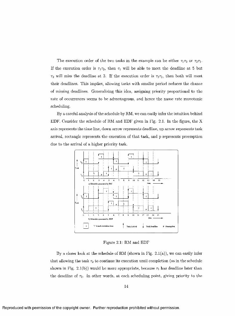
EDF. Consider the schedule of RM and EDF given in Fig. 2.1. In the figure, the X

axis represents the time line, down arrow represents deadline, up arrow represents task

arrival, rectangle represents the execution of tha t task, and p represents preemption

due to the arrival of a higher priority task.

I rn 1p 1

0 1 2 3 4 5 6 7 8 9 10 11 12 13 14 15

a) S ch ed u le generated b y R M t'*1*

T.v2

'1

0 1 5 7 8 10 11 12 13 14 152 3 4 6 9

b ) S chedu le generated by ED F

□ "t" is task execution tim e | T ask A rrival jT ask A rrival 1 T ask D ead lin e P Preem ption

Figure 2.1: RM and EDF

By a closer look at the schedule of RM (shown in Fig. 2.1(a)), we can easily infer

that allowing the task r 2 to continue its execution until completion (as in the schedule

shown in Fig. 2.1(b)) would be more appropriate, because T\ has deadline later than

the deadline of r2. In other words, at each scheduling point, giving priority to the

14


task with earliest deadline seems to be advantageous. This is the intuition behind

EDF scheduling. These two algorithms are extensively studied and widely used in

practice, and we list the main points of comparison between RM and EDF discussed

in the literature.

1. RM is easier to analyze and more predictable than EDF.

2. RM causes less jitter in task execution than EDF.

3. RM has less run-time overhead and more schedulability overhead1 than EDF[23].

Recently, the observations 1 to 3 are refuted for their accuracy and significance.

This paved the way for the motivation of our work on real-time scheduling in this

thesis.

Many scheduling algorithms for hard real-time systems were proposed in the lit

erature after RM and EDF, and all these algorithms are, in some sense, variations or

improvements of either RM or EDF[23, 24, 25, 26, 27, 28, 29, 30]. Schedulability anal

ysis for RM has been extensively studied in [31, 32, 33]. Least Laxity First (LLF)[24]

is a dynamic priority scheduling algorithm that assigns higher priority to tasks with

least laxity. The laxity of a task at time t is the difference between the deadline and

the amount of computation remaining to be completed at t. LLF was shown to be

optimal in [34] and it incurs more run time overhead compared to EDF. LLF is not

very popular because laxity tie results in frequent preemption until the tie breaks,

which results in poor performance[35]. Modified Least Laxity First (MLLF)[29] was

proposed to overcome the limitations of LLF. Whenever laxity tie occurs, MLFF de

fers the preemption as long as other tasks do not miss the deadline. MLFF is same as

LLF, if there is no laxity tie. EDF is clearly an online algorithm. An offline version of

earliest deadline based algorithm called Earliest Deadline as Late as possible (EDL)

was proposed in [25]. For this algorithm, the start times of tasks for a hyperperiod

need to be computed offline. Deadline Monotonic Algorithm (DM) [26] is a static

1 Assuming run-time overhead zero, the schedulability overhead for RM is strictly less than 100%,

on average is 88%, and for EDF it is 100%[23].

15


priority algorithm which was proposed to relax the assumption that deadline of a

task is equal to its period. DM is used when the deadline of a task Dj is less than its

period T). The intuition behind DM is that the task with smallest deadline span (not

necessarily with the smallest period) should be the task considered “most urgent”

and therefore assigned the highest priority. DM is same as RM when deadline of the

task is equal to its period [26]. In [27], the idea of stealing slack (some processing

time from periodic tasks without affecting their schedulability) for scheduling aperi

odic tasks were proposed. Slack stealing might delay periodic task executions. It was

first defined for RM and then adapted to EDF based algorithms. To facilitate better

responsiveness of soft tasks, a scheduling scheme called dual priority scheduling is

introduced in [28]. Dual priority scheduling runs hard tasks as late as possible when

there are soft tasks available for execution. It maintains three distinct priority bands:

Lower, Middle, and Upper. Hard tasks are assigned two priorities, one each for lower

and upper bands, and enter the lower band with preassigned promotion times. When

the promotion time is reached, the task is moved to the upper band. Soft tasks are

assigned in the middle band. Priorities in each band may be independent of priorities

in other bands, but priorities within a band is fixed in order to make the algorithm

minimally dynamic. The promotion times are computed based on worst case exe

cution times. A mixed priority algorithm, called combined static/dynamic (CSD)

algorithm, was introduced and used in Extensible Microkernel for Embedded, Real

time, Distributed Systems (EMERALDS) microkernel to obtain a balance between

RM and ED F[23]. In CSD scheduler, two queues are maintained - dynamic-priority

queue (DPQ) and static-priority queue (SPQ). DPQ has higher priority than SPQ.

DPQ is scheduled by EDF and SPQ is scheduled by RM. The tasks are assigned

fixed priority in the beginning and then partitioned between DPQ and SPQ, based

on the “troublesome” task, the longest period task tha t cannot be scheduled by RM.

DPQ contains higher priority tasks and SPQ contains lower priority tasks. The total

scheduling overhead of CSD is claimed to be significantly less than that of both RM

and EDF in [23].

16


2.3 Scheduling in Em bedded System s

As mentioned earlier, embedded Systems are a class of real-time systems in which

deadlines should be met with minimum power consumption. With the extensive use

of portable, battery-powered devices such as mp3 players, mobile phones, camcorders,

personal digital assistants everywhere (homes, offices, cars, factories, hospitals, plans

and consumer electronics), minimizing the power/energy consumption in these devices

is becoming increasingly important.

Power consumption is broadly classified into static and dynamic power consump

tions. Static power consumption is due to standby and leakage currents. Dynamic

power consumption is due to operational and switching activities in the device, which

are attributed to processor speed. Static power consumption can be reduced either

by operating above the critical speed or shutting down for a longer period of time.

Dynamic power consumption can be reduced either by slowing down speed of the

processor or shutting down the processor itself. Slowdown is achieved by dynamically

changing the speed of the processor by varying the clock frequency with the the sup

ply voltage. This is called as Dynamic Voltage Scaling(DVS) and it has to be applied

carefully without violating the timing constraints of the applications. Also, since

shutting down and waking up the processor consumes considerable power, shutdown

is advantageous only when the processor is idle for a period longer than a system

defined threshold value. Thus, the crux of designing an energy efficient strategy boils

down to:

• operating the processor above critical speed;

• s lo w in g d o w n p ro c e sso r sp e e d w h e n e v e r id le t im e is av a ila b le ; a n d

• shutting down the processor for a sufficient period of time.

This process normally involves computing:

• upcoming idle time;

17


• the optimal processor speed and the duration in which this speed to be applied.

In a normal situation, processor operates at its maximum speed. There are two

ways in which the speed can be adjusted, without violating the timing constraints

such as deadlines, to save energy:

1. Initially, the optimal processor speed is computed offline for the given task

set using the schedulability condition and then this speed is applied as the

maximum speed. That is, the lowest possible clock speed that satisfies the

schedulability condition; and

2. During execution, the optimal speed is computed dynamically and used when

ever there is a idle time available due to earlier completion of the task.

Earlier works were mainly focused on reducing dynamic power consumption [36,

37, 38, 39] and later approaches aimed at reducing both static and dynamic power

consumptions[40, 19, 41, 42], The algorithms proposed in [36, 40] operate the proces

sor at full speed at normal case and applies slowdown when there is a idle time in the

system, to save energy. In Low Power Fixed Priority Scheduling (LPFPS), processor

is shutdown if there are no active tasks or adopt the speed such that the current ac

tive task finishes at its deadline or the release time of the next task [36]. In [40], idle

energy consumption is reduced by extending the duration of idle periods and busy

periods for both RM and EDF. Here, the task is delayed by a small interval whenever

the task arrives during the shutdown period of the processor. The amount of delay

are computed based on schedulability condition and worst case response analysis.

The algorithms proposed in [38, 37, 39, 41, 42, 19] adjust processor speed both

initially and during execution to save energy. Cycle conserving RM (ccRM) [38]

uses schedulability condition for RM to calculate maximum constant speed in offline

phase. In the online phase of ccRM, the slack time due to earliest arrival time of

the next task is later than the worst-case completion of currently activated task is

used to adjust the speed at run-time. However, ccRM does not use the slack time

due to earlier completion of the task which results in inefficient slack estimation

18


method and inability to use lower speeds. A complex heuristic slack estimation was

proposed in [37] to overcome the disadvantage of ccRM which calculates the lowest

speed whenever the task completes earlier than the worst case execution time. In

[39], the minimum constant voltage (or speed) needed to complete a set of tasks is

obtained. Then, a voltage schedule is produced that always results in lower energy

consumption compared to using minimum constant voltage.

The techniques to reduce static power consumption are proposed in [40] and [41].

In [40, 41], the processor operates either above the critical speed or shutdown for

a sufficient period of time. The sufficient period was obtained by delaying the task

executions to reduce idle energy consumption. It was shown in [41], that the rules

to delay the task execution in [40] does not guarantee the deadline of all tasks. Pro

crastination scheduling[41] guarantees the deadlines of all tasks and reduces the idle

energy consumption. In [42], an algorithm was proposed to compute task slowdown

factors based on the contribution of the processor leakage and standby energy con

sumption of the resources in the system. In [19], DVS mechanism was proposed for

preemption threshold scheduling (PTS). Energy savings were obtained in [19] due

to reduction of preemptions in PTS. The problem of DVS in the presence of task

synchronization has been addressed in [43]. The slowdown factors for the tasks are

computed based on shared resource access and the worst execution execution time of

tasks are partitioned into critical and non-critical section. Here, the critical section

part of the task is executed at a maximum speed and the non-critical section of a

task have uniform slowdown processor speed.

2.4 Summary

In this chapter, we discussed related background for scheduling in general purpose

computing system, real-time system, and embedded system. Also, the surveys of

the related works were presented. With this background, next we will present the

simulation systems that we used to study our scheduling algorithms.

19


Chapter 3

Simulator for Scheduling

Algorithm s

This chapter presents discrete event simulators that we developed to study our schedul

ing algorithms.

3.1 Sim ulation

Simulation is a process of emulating or imitating of a system under study. The system

may be physical, logical or hypothetical one. In computer simulation, system behav

ior is modeled as the change of system states over time. In simulation systems, this

time is called simulation time. If the change of state variables is modeled as contin

uous (normally using a set of mathematical equations), then the simulation is called

continuous simulation. If the system behavior is modeled as the change of its state

at discrete points in time, then the simulation is called discrete simulation. Discrete

simulation can be further classified into time-stepped and event-driven based on the

advancement of simulation time. In event-driven simulation, the system behavior is

modeled as the change of state at the occurrence of events in the system. We use

discrete-event simulation to study scheduling systems. Three main concepts, system

states, system events, and simulation time form the basis of a discrete-event simula-

20


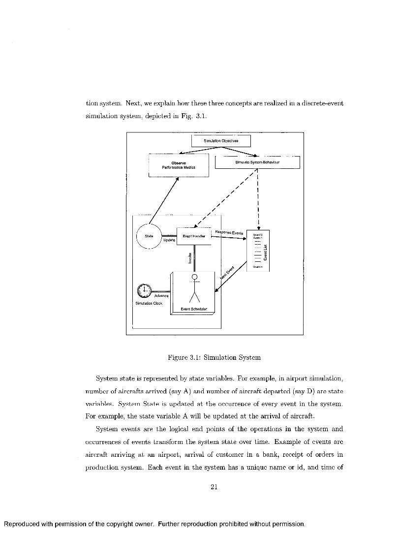
tion system. Next, we explain how these three concepts are realized in a discrete-event

simulation system, depicted in Fig. 3.1.

Simulation Objectives

Simulate System BehaviourObservePerformance Metrics

Response EventsState Event Handler

Update

Advance

Simulation Clock

Event Scheduler

Figure 3.1: Simulation System

System state is represented by state variables. For example, in airport simulation,

number of aircrafts arrived (say A) and number of aircraft departed (say D) are state

variables. System State is updated at the occurrence of every event in the system.

For example, the state variable A will be updated at the arrival of aircraft.

System events are the logical end points of the operations in the system and

occurrences of events transform the system state over time. Example of events are

aircraft arriving at an airport, arrival of customer in a bank, receipt of orders in

production system. Each event in the system has a unique name or id, and time of

21


occurrence. During simulation, events are maintained in a list called event list, which

is ordered by the time of occurrence of events. Normally, the system has a set of

initial events and occurrence of these events can trigger other events in the system

referred as response events. Simulation is carried out by executing the events from

the event list.

Simulation time reflects time flow of the system. Simulation clock maintains

simulation time and it is advanced to the time of occurrence of next event. This

process of advancing the simulation clock is continued until the simulation ends based

on a condition. Normally, simulation is carried out for a predefined time or until the

event list becomes empty.

An occurrence of an event in discrete-event simulation system can trigger two

main activities in the system: (i) generating response events and inserting them in

to the event list; and (ii) updating the state variables. The routine which has these

two activities is called event handler. The logic of the activities of the event handler

is mainly derived from the specification of the system behavior.

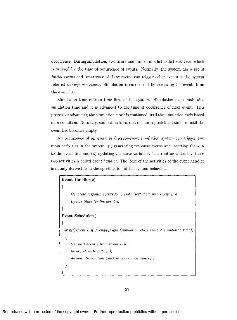
Event_Handler(e)

{Generate response events for e and insert them into Event List;

Update State for the event e;

J ___________________________________ ________________________________Event Scheduler ()

{while((Event List A empty) and (simulation clock value < simulation time))

{

Get next event e from Event List;

Invoke EventHandler(e);

Advance Simulation Clock to occurrence time of e;

}}

22


Discrete-event simulation can be described using three main components: event

list, sim ulation clock, and event scheduler. Event scheduler executes events

from event list, one by one, until either event list becomes empty or simulation time

reaches its target value. When simulation ends, the performance metrics of system

are collected from the state variables.

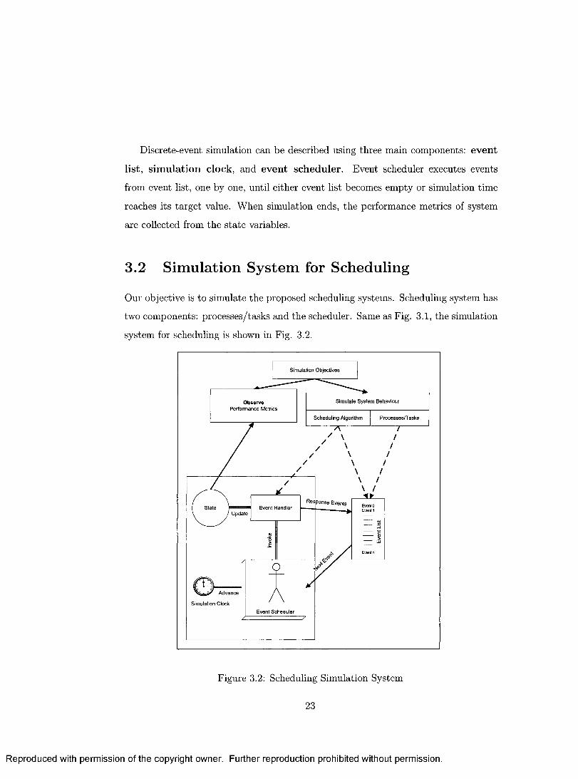
3.2 Sim ulation System for Scheduling

Our objective is to simulate the proposed scheduling systems. Scheduling system has

two components: processes/tasks and the scheduler. Same as Fig. 3.1, the simulation

system for scheduling is shown in Fig. 3.2.

Simulation Objectives

Simulate System BehaviourObservePerformance Metrics

Scheduling Algorithm Processes/Tasks

EventsEvent HandlerState

Update

Advance

Simulation Clock

Event Scheduler

Figure 3.2: Scheduling Simulation System

23


Next we discuss the list of performance metrics and events involved in the system.

3.2 .1 Perform ance M etrics

We list the performance metrics in each system.

• General Purpose Com puting System

— Turn-around time - the time interval between creation and completion of

a process.

— CPU response time - the average of the times between consecutive usage

of CPU for a process.

— Variance of turn-around time and CPU response time.

• R eal-Tim e System

— Number of preemptions.

— Deadline miss - Whenever a task is unable to complete its execution before

the deadline.

— Success ratio - the ratio of the number of feasible task sets to the total

number of task sets.

• Em bedded System

— Number of preemptions.

— Life time - the time interval between completion and activation of a task.

— Energy consumption - the amount of processor energy consumed for the

task execution.

Since events are generated from processes/tasks and the scheduler, we first discuss

the generation of processes and tasks.

24


3.2 .2 G en eration o f P rocesses

We built a process generator routine to generate the processes. It generates each pro

cess as a tuple: < process -id, arrival-time, CPU dim e, {IO-occurrence, 1 0 jw ait),

{10-occurrence, 1 0 -w a it) ,(IO -o ccu rre n ce , IO jwait) >. The value arrival-time

is generated from Poisson distribution for a given mean, CPU-time is generated

from uniform distribution for a given mean, and 10-occurrence and IO jw ait times

are generated from exponential distribution for a given mean and standard deviation.

So, the inputs for the process generator are:

• number of processes, n;

• mean values for Poisson and uniform distributions; and

• mean and standard deviation for exponential distribution.

3 .2 .3 E vents in G eneral P u rp ose C om p uting S ystem

The events in our system are generated from processes and the scheduler during

scheduling. Process_start event places the process in the ready queue for execution.

The scheduler generates CPU_assignment event and that in turn triggers any one of

the three events: process_completion event, quantum_expiry event and l / 0 _request

event. I/0_request event triggers I/0_completion event. Quantum_expiry event and

1/0-completion event will trigger CPU_assignment event. These events are summa

rized in Table 3.1.

3.2 .4 G en eration o f Tasks

We built a task generator routine to generate the task sets. Task set contains set of

tasks and each task in the task set is a tuple: < task-id, CPU-time, deadline, period >.

The values CPU -time and period are generated from uniform distribution for given

mean values. So, the inputs for the task generator are:

• number of task sets, n; and

25


Table 3.1: Events in General Purpose Computing System

Events Response Events

process_start

CPU_assignment

quantum_expiry

I/O-request

I/0_completion

process_completion

l / 0 _request, process_completion, quantum_expiry

CPU_assignment

I / O_completion

CPU_assignment

• mean values for uniform distributions

Table 3.2: Events in Real-Time and Embedded Systems

Events Response Events

task_activation

CPU_assignment

task_completion

deadline_miss

higher_priority_task_arrival

timer_expiry

CPU-assignment

task_completion, deadline_miss

task_activation

task_activation

CPU_assignment

task_activation

3 .2 .5 E vents in R ea l-T im e and E m bedded S ystem s

The events in our system are generated from tasks and the scheduler during schedul

ing. Task_activation event places the task in the ready queue for execution. The

scheduler generates CPU_assignment event and that in turn triggers any one of the

two events: task-completion event and deadline_miss event. Deadline_miss event and

timer_expiry event triggers task_activation event. Higher_priority_task_arrival event

triggers CPU-assignment event. These events are summarized in Table 3.2.

26


3.3 Sum mary

In this chapter, we discussed key concepts and ideas behind discrete event simulation.

The simulation experiments and result analysis will be presented in chapters 4, 5, and

6 .

27


Chapter 4

Fair-Share Round Robin C PU

Scheduling Algorithm s

This chapter presents our contribution to CPU scheduling for traditional interactive

operating systems. We introduce the system model in Section 4.1 and discuss round

robin scheduling and its fairness limitation in Section 4.2. In Section 4.3, a general

framework for fair-share round robin (FSRR) is introduced first and then some inter

esting versions of FSRR scheduling are derived. A simulation study of a selected set

of FSRR algorithms is presented in Section 4.4.

4.1 System M odel and Problem Statem ent

We consider the system with single processor (CPU), a scheduler, and a set of pro

cesses competing for CPU. At a time only one process can use the CPU. The problem

is to design a scheduling policy that the scheduler can use to allocate the CPU to

the processes in the system in a fair and effective manner. All the processes in the

system have equal priority to use the CPU.

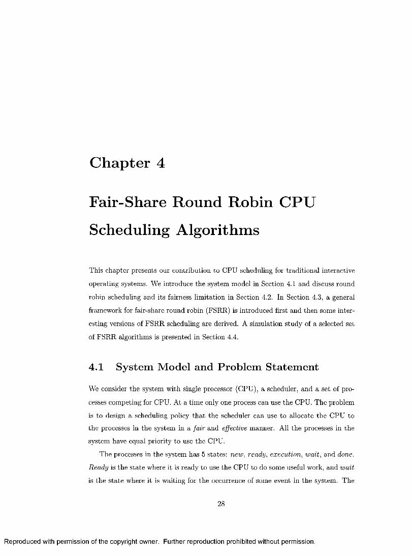
The processes in the system has 5 states: new , ready, execution, wait, and done.

Ready is the state where it is ready to use the CPU to do some useful work, and wait

is the state where it is waiting for the occurrence of some event in the system. The

28


event could be an I/O completion, a message transfer across the network, a lock or

semaphore acquirement, etc. A process is in the state execution when it is using the

CPU. Whenever a process completes its execution, it changes its state to done and

leaves the scheduling system. Process state transition diagram is given in Fig. 4.1.

Ready (R)

DoneExecutionNew

Wait (W)

Figure 4.1: State Transition Diagram

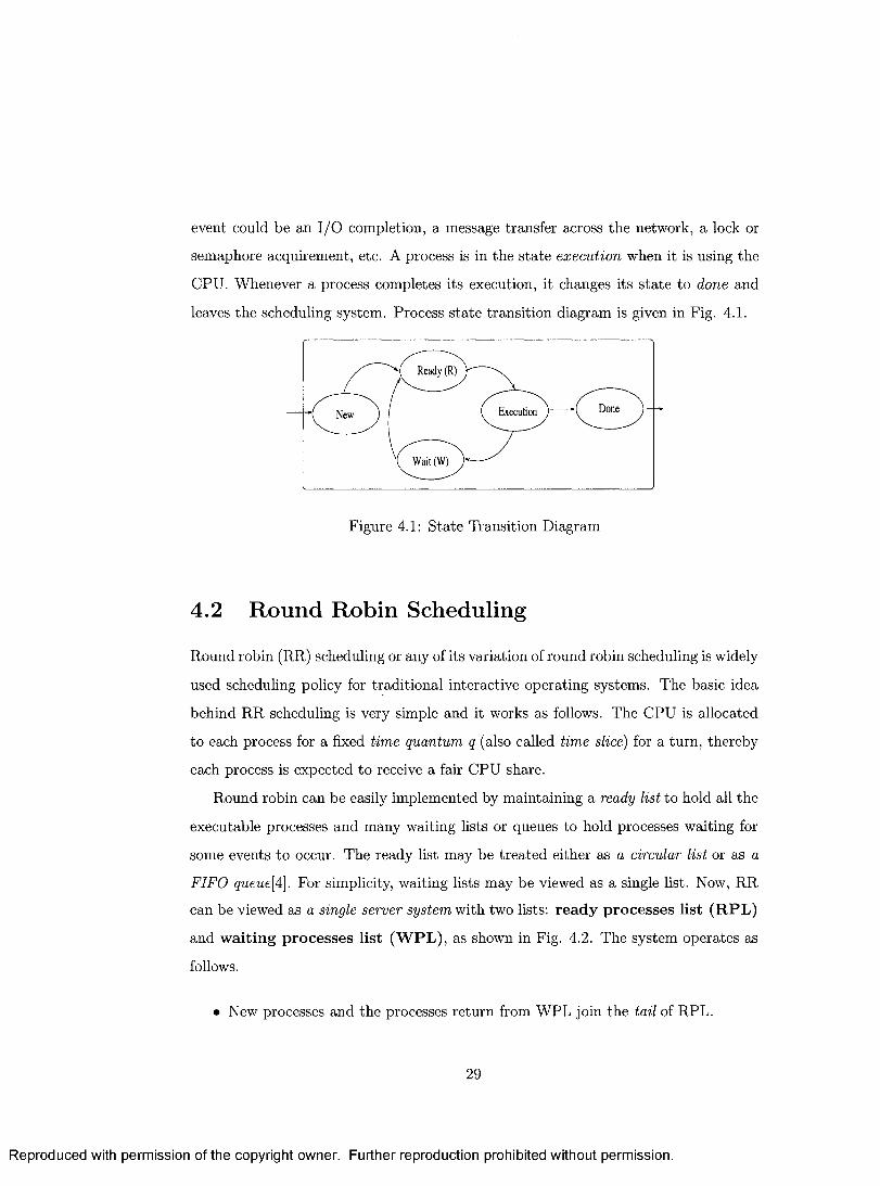
4.2 Round Robin Scheduling

Round robin (RR) scheduling or any of its variation of round robin scheduling is widely

used scheduling policy for traditional interactive operating systems. The basic idea

behind RR scheduling is very simple and it works as follows. The CPU is allocated

to each process for a fixed time quantum q (also called time slice) for a turn, thereby

each process is expected to receive a fair CPU share.

Round robin can be easily implemented by maintaining a ready list to hold all the

executable processes and many waiting lists or queues to hold processes waiting for

some events to occur. The ready list may be treated either as a circular list or as a

FIFO queue[4], For simplicity, waiting lists may be viewed as a single list. Now, RR

can be viewed as a single server system with two lists: ready processes list (RPL)

and waiting processes list (W PL), as shown in Fig. 4.2. The system operates as

follows.

• New processes and the processes return from WPL join the tail of RPL.

29


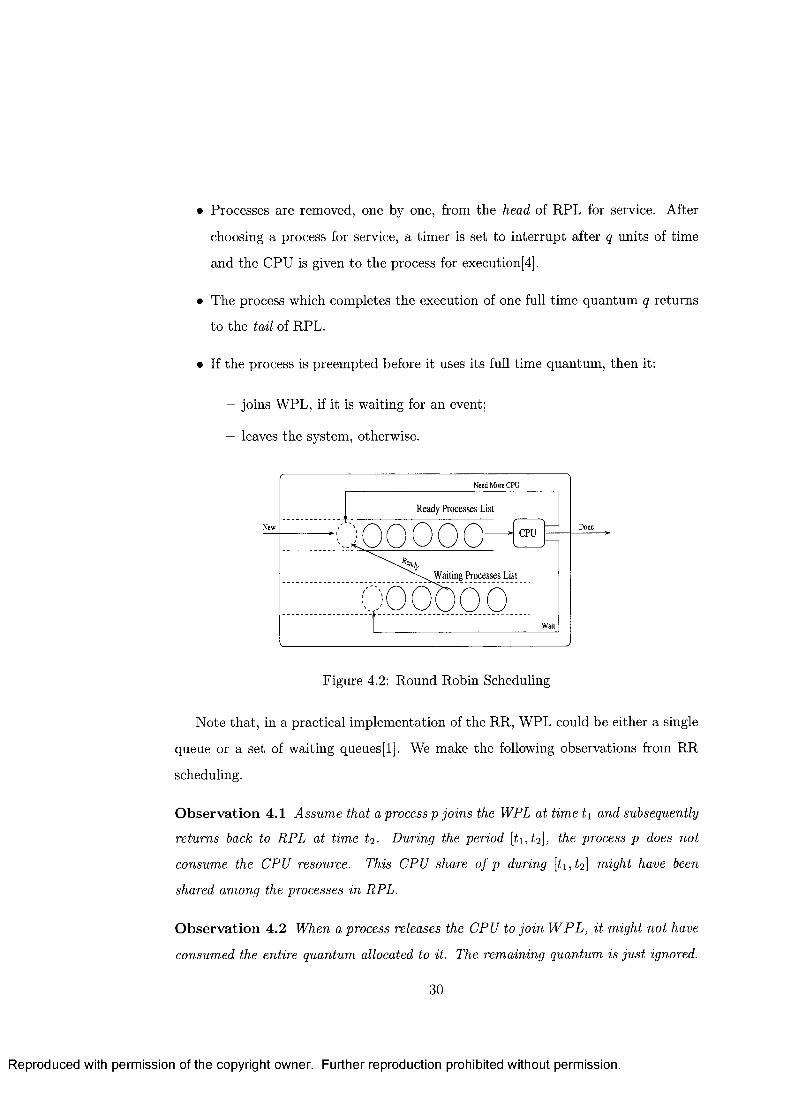
• Processes are removed, one by one, from the head of RPL for service. After

choosing a process for service, a timer is set to interrupt after q units of time

and the CPU is given to the process for execution[4],

• The process which completes the execution of one full time quantum q returns

to the tail of RPL.

• If the process is preempted before it uses its full time quantum, then it:

- joins WPL, if it is waiting for an event;

- leaves the system, otherwise.

Need More CPU

Ready Processes ListDoneNew CPU

W aiting Processes List

Wait

Figure 4.2: Round Robin Scheduling

Note that, in a practical implementation of the RR, WPL could be either a single

queue or a set of waiting queues [1]. We make the following observations from RR

scheduling.

Observation 4.1 Assume that a process p joins the WPL at time ti and subsequently

returns back to RPL at time t2 - During the period [ti,t2], the process p does not

consume the CPU resource. This CPU share of p during [U,^] might have been

shared among the processes in RPL.

Observation 4.2 When a process releases the CPU to join W P L , it might not have

consumed the entire quantum allocated to it. The remaining quantum is just ignored.

30


Observation 4.3 When a process moves from RPL to WPL, it loses it position in

the RPL; and when it returns from WPL to RPL, it is always put at the end of RPL.

The Observations 4.1, 4.2, and 4.3 illustrate the type of unfairness in sharing the

CPU attributed in RR.

4.3 Fair-Share Round Robin Scheduling (FSRR)

We informally describe the basic idea behind FSRR before it is formally characterized

subsequently.

4.3 .1 Inform al D escrip tion

The main objectives of FSRR are derived from Observations 4.1, 4.2, and 4.3, as

follows:

(a) Each process should retain its relative position in the scheduling list throughout

its life time.

(b) The loss of CPU service of a process during its wait state should be suitably

compensated in the future to assure its fair share.

The basic idea behind FSRR is the following. First, no process leaves the schedul

ing list before it consumes all the CPU resource it required. Secondly, when a process

goes to wait state it is not considered for the CPU service; instead, the scheduler

credits a specified amount of CPU time to that process in order to use it in the future

o n th e to p o f i t s r e g u la r sh a re .

The above changes from RR to FSRR bring us to two basic questions:

1 . How to compute the CPU time credits?

2. How to use the accumulated credits, in the future, on the top its regular CPU

time?

31


The scheduler could assure each process its fair share of CPU, during the process’

life time, by suitably implementing the solutions to these two questions.

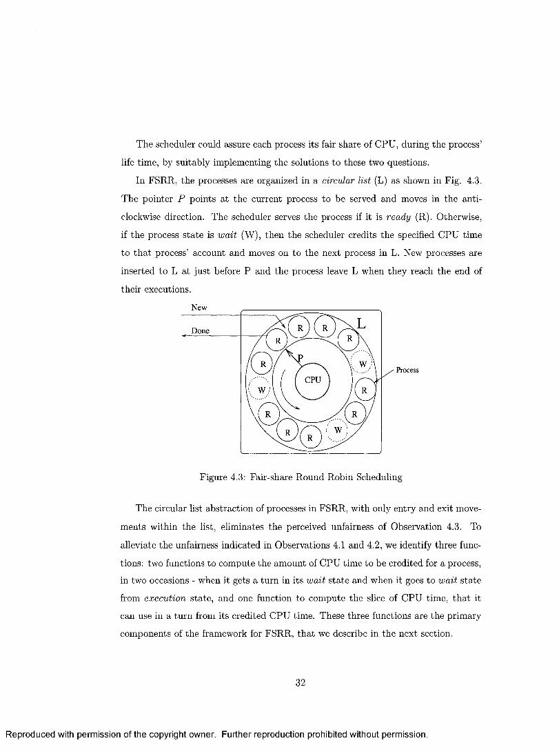
In FSRR, the processes are organized in a circular list (L) as shown in Fig. 4.3.

The pointer P points at the current process to be served and moves in the anti

clockwise direction. The scheduler serves the process if it is ready (R). Otherwise,

if the process state is wait (W), then the scheduler credits the specified CPU time

to tha t process’ account and moves on to the next process in L. New processes are

inserted to L at just before P and the process leave L when they reach the end of

their executions.

New

Done

ProcessCPU

w;

Figure 4.3: Fair-share Round Robin Scheduling

The circular list abstraction of processes in FSRR, with only entry and exit move

ments within the list, eliminates the perceived unfairness of Observation 4.3. To

alleviate the unfairness indicated in Observations 4.1 and 4.2, we identify three func

tions: two functions to compute the amount of CPU time to be credited for a process,

in two occasions - when it gets a turn in its wait state and when it goes to wait state

from execution state, and one function to compute the slice of CPU time, that it

can use in a turn from its credited CPU time. These three functions are the primary

components of the framework for FSRR, that we describe in the next section.

32


4.3 .2 Fram ework

We consider the Fair-Share Round Robin Scheduling (FSR R) as a quadruple

< L , 5, Fq, S >, where

L : the list of processes competing for the CPU service. The processes are ar

ranged in a logical circle. Initially, a pointer P is set at the first process joined

in L.

- New processes join L at the position just before P.

- Each process i in L has the following scheduling parameters:

qi : the quantum value.

Si : the state.

Ci : the credit value.

8 : the default quantum value.

Fq : the functions to com pute the quantum. The functions to compute the

quantum is a triple < f wq, f uq, f cr >, where

f wq : a real valued function which computes the amount of CPU time to be

credited for a given process when it gets a turn while it is in wait state.

f uq : a real valued function which computes the amount of CPU time to be

credited for a given process when it goes to wait state from execution

state. This is based on the unused quantum of tha t process in that turn.

f cr : a r e a l v a lu e d fu n c tio n w h ic h c o m p u te s th e a m o u n t o f CPU t im e t h a t a

process can use in a turn from its credited CPU time, in addition to its

current CPU time allocation.

S : the scheduler, which serves the process i in L at position P as follows.

- If Si = wait, then

33


* U • U T fwqi.'i')'

— If Si = ready, then

* If q > f cr(i), then qi := 8 + f cr(i) and q := a - f cr(i)-

* Else qi := 8 + Ci and c* := 0.

* Assign the CPU to i, for q, units of time.

* Wait for the CPU to return.

— When the CPU is returned to the scheduler:

* If Si = done, then remove i from L. Now P is set to its previous

position in L.

* If Si = wait, then c* := q + f uq{i)•

— Move P one position anti-clockwise.

The dynamics and the fairness of the scheduling algorithms derived from this

framework mainly depends on the functions f wq(), f m (), and / cr(). Next we present

the properties of these three functions.

P ro p e r ty 4.1 Vi, f wq(i) > 0, f uq(i) > 0.

Property 4.2 Vi, 0 < f cr(i) < c* if Ci > 0, f cr(i) = 0 if Ci = 0.

Next, we identify some concrete f wq(), f uq(), and f cr() functions.

For a given process i,

• fwq{i) may be computed as follows.

~ fwq{i) — ce8 , where a > 0 .

• fug(i) may be computed in one of the following ways.

— fuq(i) ■— fie, where a is the unused CPU time from the given q.t in that

turn and f3 > 0.

34


— fuq(i) := 7<5, where 7 > 0 .

• fcr(i) may be computed in one of the following ways.

— fcr(J-) = Ci-

— fcr{i) = k 8 , where 0 < k5 < Ci.

— fcr(i) = nnS, for the nth usage of the CPU time from c*, where 0 < nnS <

Ci. For example, assume that ct = 50 time units, 8 = 10 time units and

k = .5 time units. Then the process i will use 5 units first time, 10 units

second time, 15 units third time, and 20 units fourth time from c*.

— /cr(*) = 7 7 j f°r the nth usage of the CPU time from q , where 0 < ^ < c .

Note that 8 is a fixed parameter and a is a variable parameter that could take

any value between 0 and 8 .

4.3 .3 R R vs. F S R R

If all the processes are CPU-bound, and for each process i, f wq(i) = 0, f uq(i) — 0,

and f cr{i) = 0 in FSRR, then R R & F SR R . We explain the conceptual distinction

between RR and FSRR using the following analogy. Consider RR and FSRR as two

public view-cast stations that broadcast people’s views on various matters.

In RR, anyone who wants to express a point of view has to follow the FIFO queue

to reach the camera to express the view. Each user will be given a fixed amount of

time in a turn to express the view. A person requiring more time has to join the end

of the queue for the next turn. In this scheme, only the people who are ready with

their views are allowed to be in the queue.

In FSRR, the interested people are organized to sit in a circular fashion and the

camera is brought to them to express their views one by one. If some body is not

ready to express their view, then the chance is given to the next ready person. In

this scheme, the amount of time allowed for a person per turn may depend on the

amount of time used in the past by tha t person. Also, the participants retain their

35


relative positions in the circle throughout their sessions and the circle shrinks when

some one leaves and expands when some one joins.

4 .3 .4 F S R R A lgorith m s

Many algorithms can be derived with various combinations of the functions f wq(), f uq (),

and fcrQ- We present only a selected set of algorithms.

A l: f Wq(i) ■= 0, fuq(i) '■= 0, fcr '■= 0. This algorithm is very similar to RR. The

only difference is that this version preserves the relative positions of the pro

cesses, even if they are in wait state.

A2: f wq{i) 0, f uq{i) cr, f cr Ci. In this algorithm, only a (the unused

CPU time in that turn) is credited when the process goes to wait state from

execution state and uses 8 + c* when returns to ready state and gets its turn.

This algorithm might perform similar to V R R . The main difference is that, in

V R R Ci is given immediately after it return to ready state and gets 8 only in

the subsequent turn.

A3: f wq{i) := 8 ,fuq{i) := 0, /„. := q . In this algorithm, only the full default

quantum is credited when it gets its turn while in wait state and no CPU time

is credited when it goes to wait state from execution state. The entire credit

is allowed to use at a time in the future. This might affect the interactiveness

of other processes.

A4: f wq(i) := 8 ,fuq(i) := o , f cr := Q. In this algorithm, the full default quan

tum is credited when it gets its turn while in wait state and the remaining CPU

time a is credited when it goes to wait state from execution state. The entire

credit is allowed to use at a time in the future. Again, this might affect the

interactiveness of other processes.

A5: f wq(i) := 8 ,fuq(i) := 0, f cr '■= 8. In this algorithm, only the full default


36


is credited when it goes to wait state from execution state. The maximum 5 is

allowed to use from the credit at a time to facilitate interactiveness.

A6: f wq(i) := 5, f Uq{i) '■== cr, fcr{i) '•= In this algorithm, the full default quan

tum is credited when it gets its turn while in wait state and when it goes to

wait state from execution state and the remaining CPU time a is credited. The

maximum 5 is allowed to use from the credit at a time to facilitate interactive

ness.

A7: f wq{i) \= | , f Uq{ i ) := Oj/cr(*) :=: <k- In this algorithm, one half of the de

fault quantum is credited when it gets its turn while in wait state and no CPU

time is credited when it goes to wait state from execution state. The entire

credit is allowed to use at a time in the future. This might affect the interac

tiveness of other processes.

A8: f wq(i) := f , fuq(f) c, fcr{i) <k- In this algorithm, one half of the de

fault quantum is credited when it gets its turn while in wait state and the

remaining CPU time a is credited when it goes to wait state from execution

state. The entire credit is allowed to use at a time in the future. This might

affect the interactiveness of other processes.

A9: f wq( i ) := | , f Uq{i) 0, f c r i f ) ’■= In this algorithm, one half of the default


is credited when it goes to wait state from execution state. The maximum 5 is

allowed to use from the credit at a time to facilitate interactiveness.

AlO: fwqO := f , fuqO := o-, /„.(?') := S. In this algorithm, one half of the de



state. The maximum 6 is allowed to use from the credit at a time to facilitate

interactiveness.

37


A l l : f wq{i) | , f uq(i) '■= 0, f cr(i) ■= §■ In this algorithm, one half of the de

fault quantum is credited when it gets its turn while in wait state and no CPU

time is credited when it goes to wait state from execution state. The maximum

| is allowed to use from the credit at a time to facilitate interactiveness.

A 1 2 : f wq(i) := | , /«<?(*) := cr, f cr(i) := | . In this algorithm, one half of the de



state. The maximum | is allowed to use from the credit at a time to facilitate

interactiveness.

4.4 Sim ulation Study

In this chapter, we are interested in studying three performance metrics: average

turn-around time, average CPU response time, and standard deviation for these two

metrics. We simulated RR, A l, A2 , and A6 of FSRR to observe the above metrics

which were defined in chapter 2 .

The simulation environment is characterized by a balanced mix of CPU-bound and

I/O-bound processes that is, half of the processes are CPU-bound and the rest half

are I/ O-bound processes based on the processor-sharing model [44]. We assume that

CPU-bound processes performs no I/O operations whereas in I/O-bound processes

the I/O occurs exponentially within the CPU time.

4.4 .1 E xp erim en ta l Setup

The parameters for simulation are set as follows.

• The total number of processes in the system is denoted by N and varies from

100 to 500.

• The CPU times of processes is denoted by cpu and is uniformly distributed

between 50ms and 100ms.

38


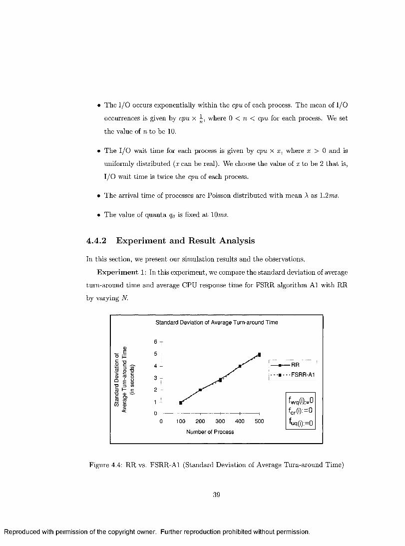
• The I/O occurs exponentially within the cpu of each process. The mean of I/O

occurrences is given by cpu x where 0 < n < cpu for each process. We set

the value of n to be 1 0 .

• The I/O wait time for each process is given by cpu x x, where x > 0 and is

uniformly distributed (x can be real). We choose the value of a; to be 2 that is,

I/O wait time is twice the cpu of each process.

• The arrival time of processes are Poisson distributed with mean A as 1.2ms.

• The value of quanta qo is fixed at 10ms.

4 .4 .2 E xperim ent and R esu lt A n alysis

In this section, we present our simulation results and the observations.

E x p erim en t 1: In this experiment, we compare the standard deviation of average

turn-around time and average CPU response time for FSRR algorithm Al with RR

by varying N.

Standard Deviation of Average Turn-around Time

— ■— RR

•-■•••FSRR-A1

100 200 300 400 500

Number of Process

Figure 4.4: RR vs. FSRR-A1 (Standard Deviation of Average Turn-around Time)

39


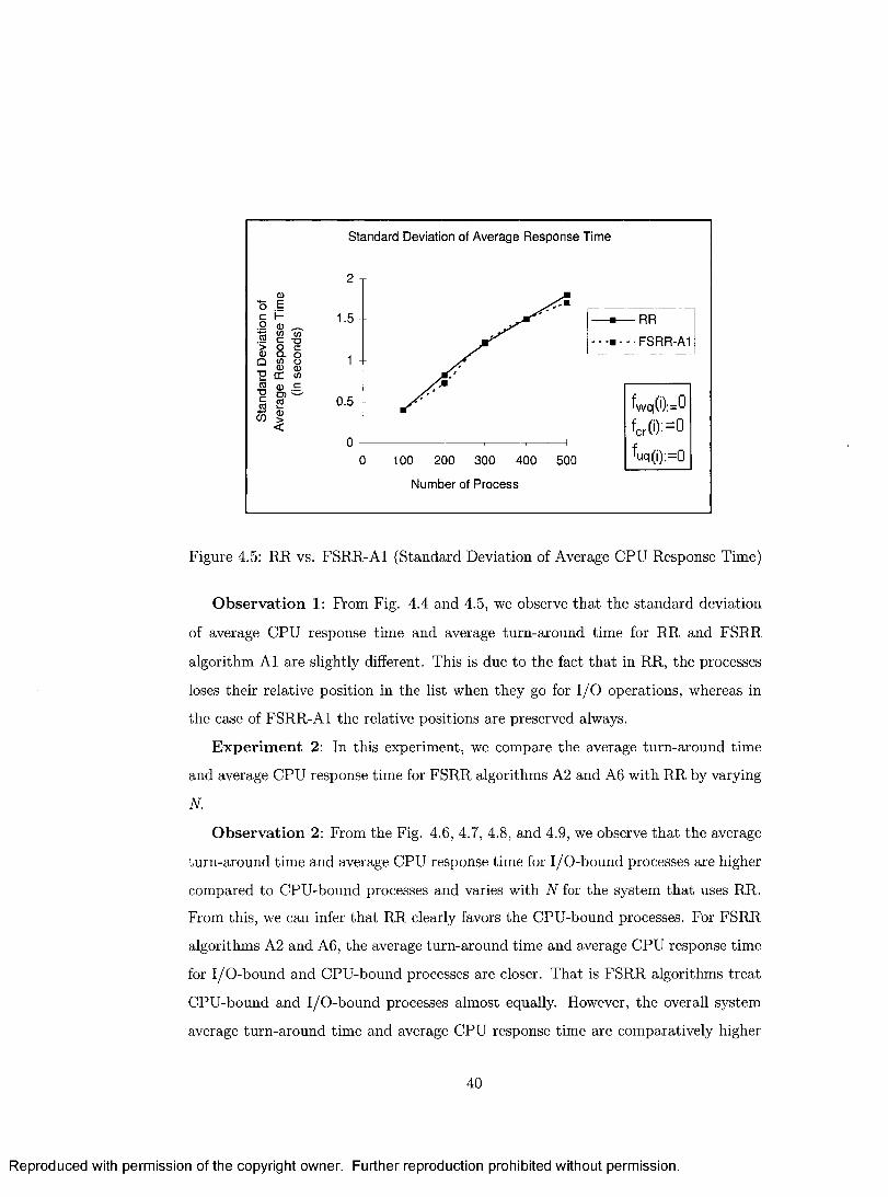
Standard Deviation of Average Response Time

RR

■ FSRR-A19- o

O) ' 0.5

100 200 300 400 500

Number of Process

Figure 4.5: RR vs. FSRR-A1 (Standard Deviation of Average CPU Response Time)

O bservation 1: From Fig. 4.4 and 4.5, we observe tha t the standard deviation

of average CPU response time and average turn-around time for RR and FSRR

algorithm A l are slightly different. This is due to the fact that in RR, the processes

loses their relative position in the list when they go for I/O operations, whereas in

the case of FSRR-A1 the relative positions are preserved always.

E x p erim en t 2: In this experiment, we compare the average turn-around time

and average CPU response time for FSRR algorithms A2 and A6 with RR by varying

N.

O bserva tion 2: From the Fig. 4.6, 4.7, 4.8, and 4.9, we observe tha t the average

turn-around time and average CPU response time for I/O-bound processes are higher

compared to CPU-bound processes and varies with N for the system that uses RR.

From this, we can infer that RR clearly favors the CPU-bound processes. For FSRR

algorithms A2 and A6 , the average turn-around time and average CPU response time

for I/O-bound and CPU-bound processes are closer. That is FSRR algorithms treat

CPU-bound and I/O-bound processes almost equally. However, the overall system

average turn-around time and average CPU response time are comparatively higher

40


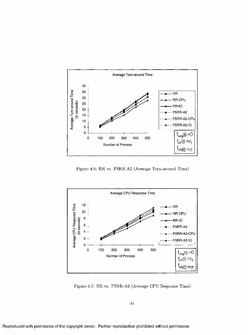
Average Turn-around Time

40 T

35 RR-oC ^ - s 3 (0 ncO T5 25 -

RR-CPU

RR-IO

- ■ FSRR-A2

- - • FSRR-A2-CPUO)- • FSRR-A2-I0

100 200 300 400 500

Number of Process

Figure 4.6: RR vs. FSRR-A2 (Average Turn-around Time)

Average CPU Response Time

RR

RR-CPU

RR-IO

- ■ FSRR-A2

- • FSRR-A2-CPUO ~o>

- ■ FSRR-A2-IO

300 400 500100 200

Number of Process

Figure 4.7: RR vs. FSRR-A2 (Average CPU Response Time)


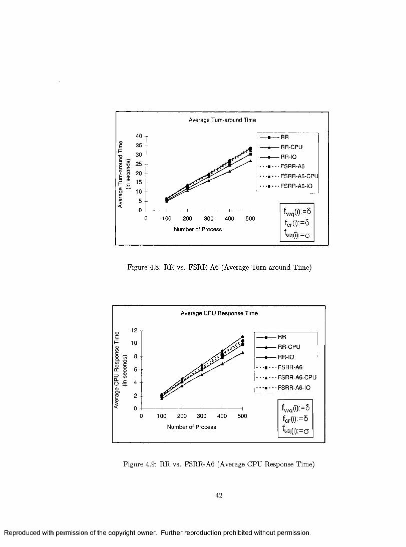
Average Turn-around Time

40

| 25 -

§ 20 <D

“ 1 5 -

0 100 200 300 400 500

Number of Process

— ■— RR

— *— RR-CPU

— • RR-IO

FSRR-A6

FSRR-A6-CPU

— • - - • FSRR-A6-IO

fWq(i):=$fcr(')-- ®^uq(i):=a

Figure 4.8: RR vs. FSRR-A6 (Average Turn-around Time)

Average CPU Response Time

0E

0incoQ .V )0DC3CLO00500><

12

10

8

6

4

2

0

0 100 200 300 400 500

Number of Process

•RR

•RR-CPU

■RR-IO

-■ - - • FSRR-A6

- - FSRR-A6-CPU

-• - - FSRR-A6-IO

W 0 := 8fc r ( i) := 8

uq(i):=a

Figure 4.9: RR vs. FSRR-A6 (Average CPU Response Time)

42


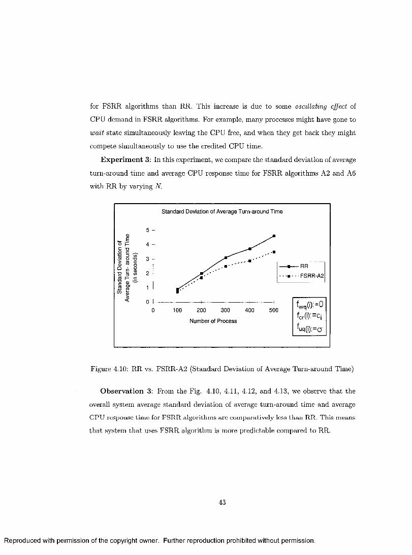
for FSRR algorithms than RR. This increase is due to some oscillating effect of

CPU demand in FSRR algorithms. For example, many processes might have gone to

wait state simultaneously leaving the CPU free, and when they get back they might

compete simultaneously to use the credited CPU time.

E x p erim en t 3: In this experiment, we compare the standard deviation of average

turn-around time and average CPU response time for FSRR algorithms A2 and A6

with RR by varying N.


-a-R R- • FSRR-A2

CD

100 200 300 400 500

Number of Process


Observation 3: From the Fig. 4.10, 4.11, 4.12, and 4.13, we observe that the

overall system average standard deviation of average turn-around time and average

C P U re sp o n se t im e fo r F S R R a lg o r i th m s a re c o m p a ra tiv e ly less t h a n R R . T h is m e a n s

that system that uses FSRR algorithm is more predictable compared to RR.

43


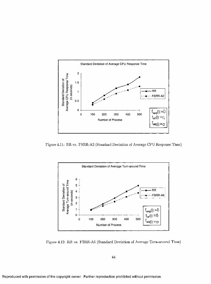
Standard Deviation of Average CPU Response Time

o wa- -9RR

■o • FSRR-A2

0.5 -o>

400 500100 200 300

Number of Process



o 1- 5 vj

«— RR

■ - - ■ FSRR-A6S ■o

500100 200 300 400

Number of Process


44


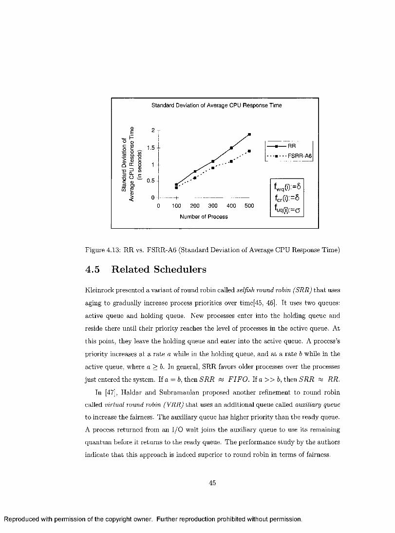
Standard Deviation of Average CPU Response Time

RR

-■ - - FSRR-A6■o

0.5O)

100 200 300 400 500

Number of Process


4.5 R elated Schedulers

Kleinrock presented a variant of round robin called selfish round robin (SRR) tha t uses

aging to gradually increase process priorities over tim e[45, 46]. It uses two queues:

active queue and holding queue. New processes enter into the holding queue and

reside there until their priority reaches the level of processes in the active queue. At

this point, they leave the holding queue and enter into the active queue. A process’s

priority increases at a rate a while in the holding queue, and at a rate b while in the

active queue, where a > b. In general, SRR favors older processes over the processes

just entered the system. If a — b, then S R R « F IF O , li a » b, then S R R ps RR.

In [47], Haidar and Subramanian proposed another refinement to round robin

called virtual round robin (VRR) tha t uses an additional queue called auxiliary queue

to increase the fairness. The auxiliary queue has higher priority than the ready queue.

A process returned from an I/O wait joins the auxiliary queue to use its remaining

quantum before it returns to the ready queue. The performance study by the authors

indicate tha t this approach is indeed superior to round robin in terms of fairness.

45


Many multilevel feedback (MLF) based scheduling algorithms favor I/O-bound

processes over CPU-bound processes[48, 49, 1, 3, 2, 4, 50]. In this class, the I/O-

bound processes generally gets higher priority when they returned from I/O wait [49].

MLF scheduling has the advantage of having flexible control over various processes.

On the other hand, it is also the most complex[4].

The scheduler employed in Linux[49, 51] maintains two basic classes of threads:

real-time and regular. Real-time threads are assigned fixed priorities, always greater

than the priorities of regular threads and their priorities are computed at each epoch.

An epoch ends when no threads are ready to execute. The current priority of a regular

process is translated into the quantum value that it can use in tha t epoch. Each thread

is assigned a base quantum at the time of creation. The quantum value for the next

epoch is computed as the sum of the base quantum and half of its remaining quantum

from the previous epoch. This naturally favors I/O-bound threads[49, 51].

The basic scheduling principles of Windows 2000 and VAX/VMS are the same,

except tha t Windows schedules threads whereas VAX/VMS schedules processes [49].

Here, whenever a thread returns from its wait state, it gets a boost according to the

event it was waiting for. For example, a thread waiting for disk I/O will get a boost

of 1, whereas a thread waiting for a mouse or keyboard interrupt gets a boost of 6.

Hence, I/O-bound threads are favored when they returned from I/O wait.

From the review of the above schedulers, it is evident that favoring I/O-bound

processes over CPU-bound processes mostly increases both the fairness among the

processes and overall system performance.

The contribution in this thesis has some similarity in generality to the work pre

sented in [52], Ruschitzka and Fabry [52] presented a generic scheme for classifying

scheduling algorithms based on an abstract model which formalizes the notion of pri

ority, whereas we present an abstract model which formalizes the fair treatment of

processes in round robin scheduling.

46


4.6 Sum mary

The simulation results confirm our assertion that the proposed class of FSRR al

gorithms with suitable selection of f wq, f Uq, and fcr reduces the variance in average

CPU response time and variance in average turn-around time and hence alleviates

the fairness issue observed in round robin.

47


Chapter 5

A ctivation Adjusted Scheduling

Algorithm s for Hard Real-Tim e

System s

This chapter presents our next contribution, which is on hard real-time scheduling.

Section 5.1 presents the system model and problem statement. Section 5.2 gives an

overview of static priority scheduling algorithms for hard real-time systems. Two

frameworks and a selected set of scheduling algorithms derived from the frameworks

are the key contributions in this chapter. The framework for Off-line Activation-

Adjusted Scheduling Algorithms (OAA) and a set of OAA algorithms have been

presented in Section 5.3. Subsequently, Section 5.4 presents the framework for Adap

tive Activation-Adjusted Scheduling Algorithms and the derivation and analysis of

AAA algorithms. A simulation study and the experimental results comparing RM

a n d E D F w ith o u r a lg o r i th m s is p re s e n te d in S e c tio n 5.5.


We consider a system with a single processor, a scheduler, and a set of n periodic

tasks. Informally, the problem is to design a scheduling policy tha t the scheduler

48


can use to determine the task to be executed at a particular moment, so that each

task in the system completes the execution before its deadline. To define the problem

formally, we introduce the following terminology.

• A periodic task r* is associated with the following parameters:

— Ti is the length of the period,

— Ci is the worst case execution time (WCET),

— Bi is the best case execution time (BCET), which is computed based on

the percentage of WCET

— Ei is the time for which n has already executed, and

— Pi is the priority.

• A set of n periodic tasks is called a task set and is denoted by T = (ri, t 2, ..., rn).

W ithout loss of generality, we assume that T\, t 2 , ..., rn are ordered by decreasing

priority, so that T\ is the highest priority task.

• The absolute periods for r, are: [0, T f, [Tt) 2T,}, [2Tt, 3Tt] , .... The end of the

periods Tj,2Tj,..., are defined as the absolute deadlines for r* in the respective

periods.

• We denote the absolute activation time for t, in the kth interval as a ^ .

• 1/Tj is defined as the request rate of the task r,.

• The ratio Ui — Ci/Ti is called the utilization factor of the task 7* and represents

the fraction of processor time to be used by that task.

We adopt the following assumptions from [8].

• All tasks are independent and preemptive.

• The priority of each task is fixed.

49


Formally, the problem is to design a scheduling algorithm tha t determines the task

to be executed at a particular moment so tha t each task r* in the system completes

its kth execution within its kth period [(k — 1)7*, kTi], Vk = 1,2,3,...

As indicated earlier, the scheduling algorithms for hard real-time system can be

classified into static priority scheduling and dynamic priority scheduling. Since our

algorithms are built based on static priority scheduling, we briefly review the basic

idea behind static priority scheduling next.

5.2 Static Priority Scheduling A lgorithm s

The basic idea behind static priority scheduling algorithms is simple:

• the priority of the tasks are assumed to be fixed throughout the execution;

• at any time, the scheduler selects the highest priority task which is ready for

execution; and

• the selected task is executed until a higher priority task arrives or until it com

pletes its execution.

An implementation scheme for fixed priority schedulers is described in [53] as follows.

The scheduler maintains essentially two queues: ready queue and wait queue. The

ready queue contains the tasks which are ready for execution and the wait queue

contains the tasks that have already completed the execution for their current periods

and are waiting for their next periods to start again. The ready queue is ordered by

priority and the wait queue is ordered by next start time.

When the scheduler is invoked, it examines the tasks in the wait queue to see if

any task should be moved to the ready queue. Then it compares the head of the

ready queue to the task currently being executed. If the priority of the task in the

head of the ready queue is higher than the priority of currently executing task, then

the scheduler invokes a context switch. The scheduler is invoked by an interrupt

50


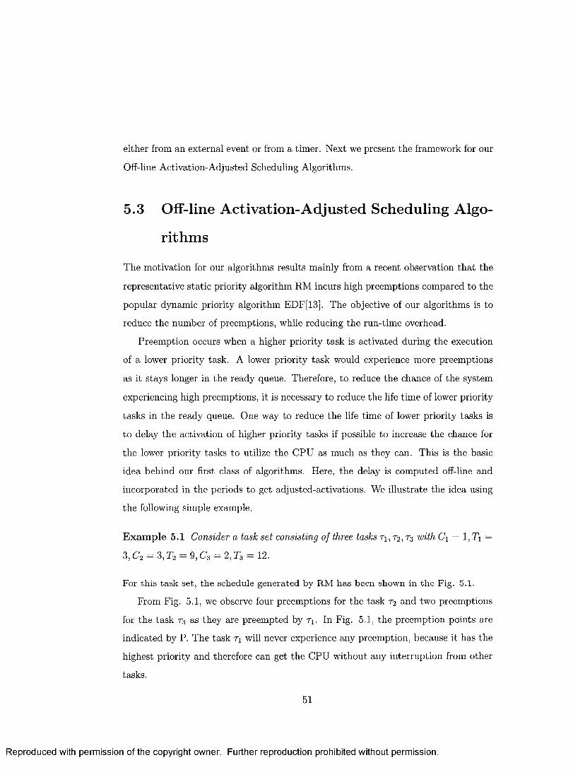
either from an external event or from a timer. Next we present the framework for our

Off-line Activation-Adjusted Scheduling Algorithms.

5.3 Off-line A ctivation-A djusted Scheduling A lgo

rithm s

The motivation for our algorithms results mainly from a recent observation that the

representative static priority algorithm RM incurs high preemptions compared to the

popular dynamic priority algorithm EDF[13], The objective of our algorithms is to

reduce the number of preemptions, while reducing the run-time overhead.

Preemption occurs when a higher priority task is activated during the execution

of a lower priority task. A lower priority task would experience more preemptions

as it stays longer in the ready queue. Therefore, to reduce the chance of the system

experiencing high preemptions, it is necessary to reduce the life time of lower priority

tasks in the ready queue. One way to reduce the life time of lower priority tasks is

to delay the activation of higher priority tasks if possible to increase the chance for

the lower priority tasks to utilize the CPU as much as they can. This is the basic

idea behind our first class of algorithms. Here, the delay is computed off-line and

incorporated in the periods to get adjusted-activations. We illustrate the idea using

the following simple example.

E xam ple 5.1 Consider a task set consisting of three tasks t\ , t2, t 3 with C\ = 1, Tj =

3,C 2 = 3,T2 = 9,C 3 = 2,T3 = 12.

F o r th is ta s k s e t, th e sc h e d u le g e n e ra te d b y R M h a s b e e n sh o w n in th e F ig . 5.1.

Prom Fig. 5.1, we observe four preemptions for the task r2 and two preemptions

for the task r3 as they are preempted by T\. In Fig. 5.1, the preemption points are

indicated by P. The task Ti will never experience any preemption, because it has the

highest priority and therefore can get the CPU without any interruption from other

tasks.

51


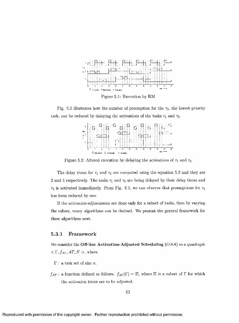
t Task A nivjl I Task Dcadliae P Preemption

Figure 5.1: Execution by RM

Fig. 5.2 illustrates how the number of preemption for the 7 3 , the lowest priority

task, can be reduced by delaying the activations of the tasks T\ and 7 2 .

□ q

n ^ m i

□ a aH -m i

a

n

q

n ^ m 1

q IR i □ I Qq - r n i

3 6 9 12 15 18 21 24 27 30 33 36

| Task Arrival | Task Deadline P Preemption

Figure 5.2: Altered execution by delaying the activations of t\ and r2

The delay times for T\ and r2 are computed using the equation 5.3 and they are

2 and 4 respectively. The tasks T\ and r2 are being delayed by their delay times and

73 is activated immediately. From Fig. 5.2, we can observe that preemptions for r3

has been reduced by one.

If the activation-adjustments are done only for a subset of tasks, then by varying

the subset, many algorithms can be derived. We present the general framework for

these algorithms next.

5.3.1 Fram ework

We consider the Off-line A ctivation-A djusted Scheduling (O AA) as a quadruple

< F, f a t , AT, S' >, where

T : a task set of size n.

f at ■ a function defined as follows. / a t {T) = II, where II is a subset of T for which

the activation times are to be adjusted.

52


A T : a set of pairs (Na>i, aiti), where N a<i is the next activation time and aiti is

the offset of activation adjustment of r*. For every task t% £ If, the absolute

activation time is computed as follows.

Qi i Ti Fti(5.1)

Q'ijk Ui,k—1 "F T{y \ / k 1

where Ri is the worst case response time of t%. Ri is calculated iteratively using

the equation 5.3.

For every task T j not in II, the absolute activation time a h k is

a ,-1 = 0(5.2)

&j ,k ^ j , k —l "f" T j , V j 1

S' : the scheduler. The scheduler component is a triple < Wq, R q, S'p >, where

Wq : a queue of tasks waiting to be activated, ordered by increasing absolute

activation time.

R q : a queue of ready tasks, ordered by decreasing priority.

S'p : the scheduling policy. The scheduler S ' can be invoked either by the com

pletion of a task or by a timer expiry. When the scheduler S' is invoked,

1. I f the invocation of S' was by the completion of a task, then

* S' places the completed task in Wq, with next activation time set.

2. Else, if the invocation of S' was by timer interrupt, then

* I f a task is interrupted by the timer, then S' places the interrupted

task in R q.

3. S ' checks Wq to see any task to be transferred from Wq to Rq and then

transfers such tasks to Rq.

4. I f R q is not empty, then

53


* Let Tj be the task in the head of Rq, with priority p. S ' scans Wq

starting from the head and identifies the first task, say r fc, with

priority greater than p.

* S ' sets the timer to rk's next activation time.

* S' schedules Tj for execution.

5. S' waits for invocation.

N ote: Wq and R q may be implemented more efficiently, as mentioned in [13], by

splitting them into several queues, one for each priority.

5.3 .2 C om p uting Ri

The worst-case response time Ri of the task r* can be computed iteratively using the

following formula[13]:

R i ( 0 ) - C i

W ) = c i + E , £Wi,

where hp(i) is the set of higher priority tasks than r,; which causes interference for

task r* and hence preempting it [54], The worst case response time of Tj is given by

the smallest value of Ri(k) such that Rj{k) = Ri{k — 1).

5 .3 .3 O A A Scheduling A lgorith m s

The idea behind OAA algorithms is in the implementations of f at in the framework.

Prom simple set theory, f AT can have 2n possible implementations. We list only a

few meaningful implementations below.

For a given task set T,

1. f AT{V) = {}

2. f AT(T) = r.

54


3- / a t ( r ) = { r i,r2, ...,rm}, where 1 < m < n .

Next we present OAA scheduling algorithms for RM assigned priorities.

5 .3 .4 O A A -R M Scheduling A lgorith m s

RM is the most used scheduling algorithm for real-time applications because it is

supported in most OS kernels[36]. The idea behind RM scheduling is priority assign

ment scheme. In RM, high frequency tasks are assumed to be of higher priority than

low frequency tasks (that is, tasks with high activation rate get higher priorities and

hence the name rate monotonic).

With RM assigned priority, many OAA algorithms can be obtained by suitably

choosing Ja t - We refer these algorithms as OAA-RM. We simulate OAA-RM3 and

compare with RM and EDF. The representative OAA-RM algorithms are:

OAA-RM1: / U t ( T ) — { } . This is same as RM.

OAA-RM2: / a t { r ) = {r i}- Only the highest priority task is delayed activa

tion.

OAA-RM3: I a t {P) — (ri, r2, .... }. The lower half of the task set is delayed

activation.

OAA-RM4: / a t {H = {'Ti,t 2 , Except the lowest priority task, all

other tasks are delayed activation.

OAA-RM5: I a t ( P ) = T. All the tasks are delayed activation.

5.3 .5 A n alysis

Compared to traditional static priority algorithms, OAA algorithms have an addi

tional off-line computation costs: Computing f at °f the task set and generating the

values of AT. This one-time cost can be justified by the reduction of run-time costs.

55


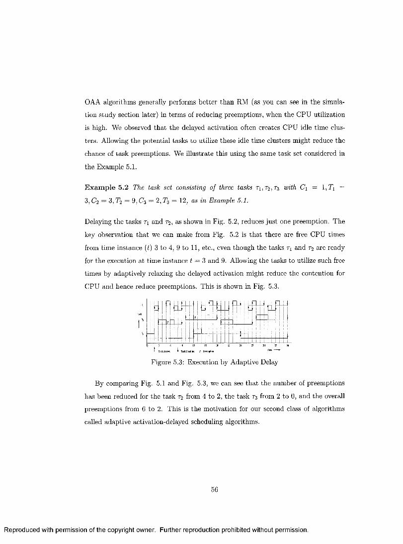
OAA algorithms generally performs better than RM (as you can see in the simula

tion study section later) in terms of reducing preemptions, when the CPU utilization

is high. We observed that the delayed activation often creates CPU idle time clus

ters. Allowing the potential tasks to utilize these idle time clusters might reduce the

chance of task preemptions. We illustrate this using the same task set considered in

the Example 5.1.

E xam ple 5.2 The task set consisting of three tasks ti,T 2 , t 3 with C\ — 1 , T) =

3, C2 — 3, T2 = 9, C3 = 2, T3 = 12, as in Example 5.1.

Delaying the tasks t\ and r2, as shown in Fig. 5.2, reduces just one preemption. The

key observation that we can make from Fig. 5.2 is that there are free CPU times

from time instance (t ) 3 to 4, 9 to 11, etc., even though the tasks ti and r 2 are ready

for the execution at time instance t = 3 and 9. Allowing the tasks to utilize such free

times by adaptively relaxing the delayed activation might reduce the contention for

CPU and hence reduce preemptions. This is shown in Fig. 5.3.

D U N

it>na o

r L

i Fa

1

tfi JU J

12 IS 18 21

Task Arrival T Task Deadline P Preemption

Figure 5.3: Execution by Adaptive Delay

By comparing Fig. 5.1 and Fig. 5.3, we can see that the number of preemptions

has been reduced for the task r 2 from 4 to 2, the task r 3 from 2 to 0, and the overall

preemptions from 6 to 2. This is the motivation for our second class of algorithms

called adaptive activation-delayed scheduling algorithms.

56


5.4 A daptive A ctivation A djusted Scheduling A l

gorithm s

The basic idea behind adaptive activation-adjusted scheduling algorithms is that the

activation of the tasks are delayed only when needed. For the sake of simplicity in

implementation, the algorithm delays the activations of all tasks to their adjusted-

activation times and then wisely revokes the delays of some tasks to utilize the free

CPU. The algorithm is same as OAA if the CPU is always busy. When the CPU

becomes free, that is when R q is empty, the scheduler looks at Wq to look for an

eligible task to schedule.

D efinition 5.1 Assume that a task has completed its kth execution and it is waiting

in Wq for its next execution. The task Ti is eligible for its next execution at time

t, if t > kTi.

Next we present the framework incorporating this idea.

5.4 .1 Fram ework

We consider the A daptive A ctivation-A djusted Scheduling {AAA) as a quadru

ple < r , f a t i AT, S" >, where


/ at '■ a function defined as follows. fx r(T ) = n , where II is a subset of T for which


A T : a set of pairs (Na<i, a^i), where Na>i is the next activation time and avl is

the offset of activation adjustment of r*. For every task r, G II, the absolute

activation time a*,* is computed as stated in OAA.

S" : the scheduler. The scheduler component is a quadruple < Wq, R q, Ap, S ” >,

where

57



activation time.

Rq : a queue of ready tasks, ordered by decreasing priority.

A p : a policy to select an eligible task from Wq to transfer to Rq. It returns

either the id of first eligible task or the id of a task which will become

eligible in the nearest future.

S'" : the scheduling policy. The scheduler can be invoked either by the comple

tion of a task or by a timer expiry. When the scheduler S" is invoked,

1. I f the invocation of S" was by the completion of a task, then

* S'" places the completed task in Wq, with next activation time set.

2. Else, if the invocation of S" was by timer interrupt, then

* I f a task is interrupted by the timer, then S'" places the interrupted

task in R q.

3. S'" checks Wq to see if any tasks are to be transferred from Wq to R q

and then transfers such tasks to R q.

4. If R q is not empty, then

* Let Tj be the task in the head of R q, with priority p. S'" scans Wq

starting from the head and identifies the first task, say rk, with


* S'" sets the timer to r fc’s next activation time.

* S" schedules Tj for execution.

5. Else1,

* S" calls Ap, and let Ap returns rk and t be the current tim e.

* If Na)k - akti > t, then

• S" transfers from Wq to R q.

1This is extra component over traditional static priority algorithms and therefore highlighted in

boldface.

58


• go to step 4.

* Else,

• S" sets the tim er to m in(tim er, Na>k — ak<i).

6. S" waits for invocation.

5.4 .2 A A A Scheduling A lgorith m s

We can derive many AAA algorithms by suitably implementing Ap and J'at from the

framework. We have listed the selection choices for Jat in section 5.3.3. Here we list

some choices for Ap.

We assume that the task search for Ap starts from the head of the Wq and returns

a task which will be eligible in the nearest future2 satisfying the following criteria:

API: The first task from Wq.

AP2: The lowest priority task in Wq.

AP3: The highest priority task from Wq.

AP4: The first lowest priority task in Wq.

AP5: The first highest priority task in Wq.

AP6: The task with minimum Ci in Wq.

AP7: The task with maximum Ci in Wq.

AP8: The task with best-fit3 Ci in Wq.

Next we present AAA-RM algorithms.

2 A task which is eligible now is also eligible in the nearest future.3The maximum Ci less than the remaining timer value.

59


5 .4 .3 A A A -R M Scheduling A lgorith m s

W ith RM assigned priority, many AAA algorithms can be obtained by suitably choos

ing f at and Ap. Some algorithms are as follows.

AAA-RM 1 I a t {r ) = { r i , 72,...,r a } and Ap = API.

AAA-RM2 / a t O " ) = { T i , T 2, . . . , r „ _ i } and Ap = API.

AAA-RM3 I a t (r ) = { t i , t 2 , . . . j T a } and Ap = API.

AAA-RM4 f AT(r) = r and Ap = API.

AAA-RM5 = r and Ap = AP2.

AAA-RM6 / yr / ’( r ) = {} and Ap = API. This behaves the same way as RM

We simulate AAA-RM4 to compare with RM and EDF.

5.4 .4 A n alysis

When compared with static priority algorithms, our AAA algorithm has an extra

run-time step (step 5 in the framework) in addition to the off-line computation of

/ a t - Note tha t the step 5 in the framework (and hence in the algorithm) will be

executed only when Rq is empty. That is, step 5 consumes only the free CPU which

otherwise would have wasted. But the benefit gained in preemption reduction due to

step 5 is significant, as witnessed in the simulation study.


For our simulation, w e b u i l t a n d u se d a J a v a b a s e d d is c re te e v e n t s im u la to r to s im

ulate the algorithms. We are interested in observing and studying the number of

preemptions, the cost involved in context switches, success ratio, average number of

deadline misses.

Context Switch is an activity of switching the CPU from one task to another task.

This activity generally involves a nonzero cost and varies from system to system,

60


based on so many factors such as cache usage, scheduler complexity, context size, etc.

However, for most analysis in the real-time systems, it is assumed as either zero or

fixed. Also, the cost varies depending upon the reason for the occurrence of context

switch: completion of the current task or request from a higher priority task.

5.5.1 T erm inology

D efinition 5.2 I f the context switch occurs due to task completion then the cost is

loading/restoring the context of the new task. We call this cost as task-sw itching

cost.

D efinition 5.3 I f the context switch occurs due to an interrupt from a higher priority

task then the cost is saving the context of the current task and loading/restoring the

context of the new task. We call this cost as preem ption cost.

We assume that this cost is constant for a task set and varies from 0% to 25% of

the mean worst case computation cost of the task set.

D efinition 5.4 The average context switch cost is the average of task-switching

cost and preemption cost.

D efinition 5.5 H yperperiod of a task set is defined as the smallest interval of time

after which the schedule repeats itself and is equal to the least common multiple of the

task periods [13].

5.5 .2 E xp erim enta l Setup

Task periods were generated uniformly in the range [10ms, 120ms] and in multiples

of 10, so that the LCM of the task set are not huge. The WCET of each task were

assigned in the range [0.5ms, 10ms].

61


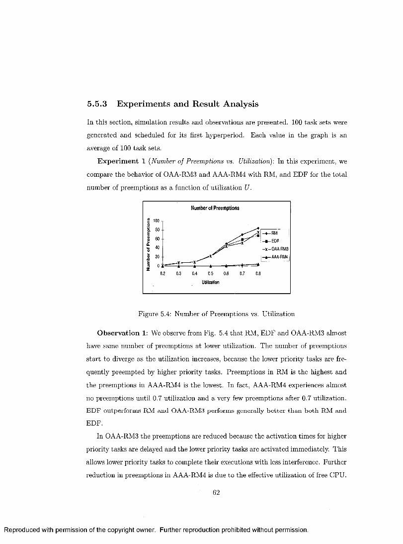
5.5 .3 E xp erim en ts and R esu lt A n alysis

In this section, simulation results and observations are presented. 100 task sets were

generated and scheduled for its first hyperperiod. Each value in the graph is an

average of 100 task sets.

Experim ent 1 (Number of Preemptions vs. Utilization): In this experiment, we

compare the behavior of OAA-RM3 and AAA-RM4 with RM, and EDF for the total

number of preemptions as a function of utilization U.

Number of Preemptions

100 T

- ♦ - R M

- ■ — EDF

-X -0 A A -R M 3

AAA-RM4

60 -

Utilization

Figure 5.4: Number of Preemptions vs. Utilization

Observation 1: We observe from Fig. 5.4 that RM, EDF and OAA-RM3 almost

have same number of preemptions at lower utilization. The number of preemptions

start to diverge as the utilization increases, because the lower priority tasks are fre

quently preempted by higher priority tasks. Preemptions in RM is the highest and

the preemptions in AAA-RM4 is the lowest. In fact, AAA-RM4 experiences almost

no preemptions until 0.7 utilization and a very few preemptions after 0.7 utilization.

E D F o u tp e r fo rm s R M a n d O A A -R M 3 p e r fo rm s g e n e ra lly b e t t e r t h a n b o th R M a n d

EDF.

In OAA-RM3 the preemptions are reduced because the activation times for higher

priority tasks are delayed and the lower priority tasks are activated immediately. This

allows lower priority tasks to complete their executions with less interference. Further

reduction in preemptions in AAA-RM4 is due to the effective utilization of free CPU.

62


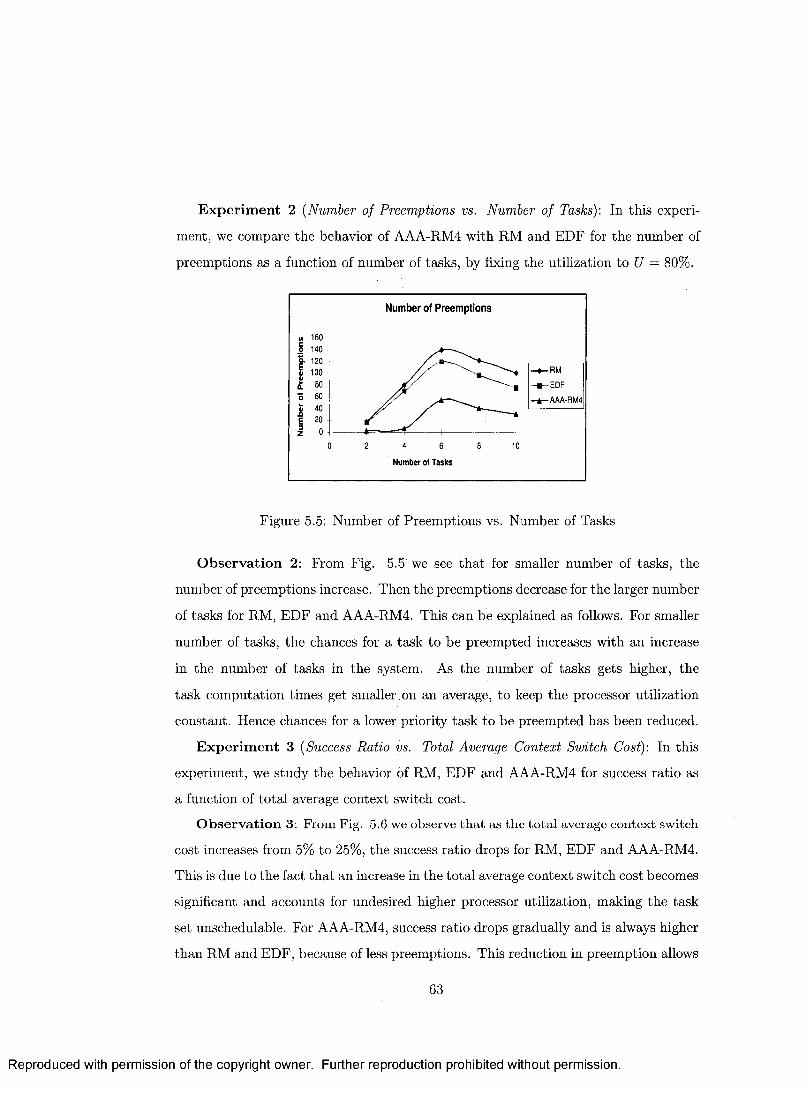
E x p erim en t 2 (Number of Preemptions vs. Number of Tasks): In this experi

ment, we compare the behavior of AAA-RM4 with RM and EDF for the number of

preemptions as a function of number of tasks, by fixing the utilization to U = 80%.

Number of Preem ptions

» 160

g- 120 -

I 100 -d>£ 80 -

RM

EDF

AAA-RM440 -

Number o< Tasks

Figure 5.5: Number of Preemptions vs. Number of Tasks

O bserva tion 2: From Fig. 5.5 we see that for smaller number of tasks, the

number of preemptions increase. Then the preemptions decrease for the larger number

of tasks for RM, EDF and AAA-RM4. This can be explained as follows. For smaller

number of tasks, the chances for a task to be preempted increases with an increase

in the number of tasks in the system. As the number of tasks gets higher, the

task computation times get smaller on an average, to keep the processor utilization

constant. Hence chances for a lower priority task to be preempted has been reduced.

E x p erim en t 3 (Success Ratio vs. Total Average Context Switch Cost): In this

experiment, we study the behavior of RM, EDF and AAA-RM4 for success ratio as

a function of total average context switch cost.

O bserva tion 3: From Fig. 5.6 w e o b se rv e t h a t a s th e t o t a l av e ra g e c o n te x t sw itc h

cost increases from 5% to 25%, the success ratio drops for RM, EDF and AAA-RM4.

This is due to the fact that an increase in the total average context switch cost becomes

significant and accounts for undesired higher processor utilization, making the task

set unschedulable. For AAA-RM4, success ratio drops gradually and is always higher

than RM and EDF, because of less preemptions. This reduction in preemption allows

63


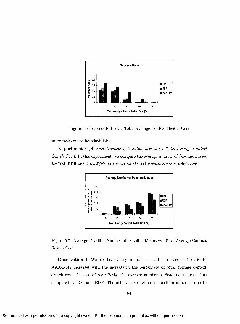
Success Ratio

o 0.8 -

|R M

■ EDF

■ AAA-RM4

5 10 15 20 25

Total Average Context Switch Cost (%)

Figure 5.6: Success Ratio vs. Total Average Context Switch Cost

more task sets to be schedulable.

E x p erim en t 4 (Average Number of Deadline Misses vs. Total Average Context

Switch Cost): In this experiment, we compare the average number of deadline misses

for RM, EDF and AAA-RM4 as a function of total average context switch cost.

Figure 5.7: Average Deadline Number of Deadline Misses vs. Total Average Context

Switch Cost

O b servation 4: We see that average number of deadline misses for RM, EDF,

AAA-RM4 increases with the increase in the percentage of total average context

switch cost. In case of AAA-RM4, the average number of deadline misses is less

compared to RM and EDF. The achieved reduction in deadline misses is due to

Average Number of Deadline M isses

250 T

■ RM

■ EDF

■ AAA-RM4

5 10 15 20 25

Total Average Context Switch Cost (%)

64


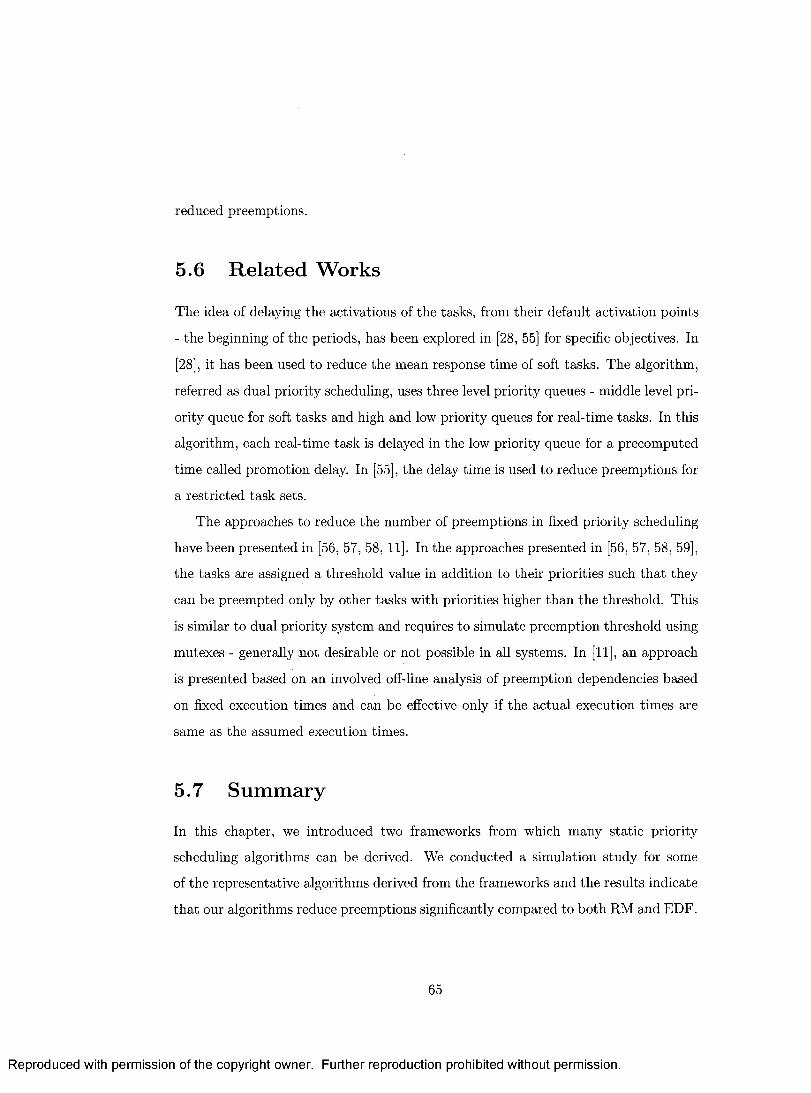
reduced preemptions.

5.6 R elated Works

The idea of delaying the activations of the tasks, from their default activation points

- the beginning of the periods, has been explored in [28, 55] for specific objectives. In

[28], it has been used to reduce the mean response time of soft tasks. The algorithm,

referred as dual priority scheduling, uses three level priority queues - middle level pri

ority queue for soft tasks and high and low priority queues for real-time tasks. In this

algorithm, each real-time task is delayed in the low priority queue for a precomputed

time called promotion delay. In [55], the delay time is used to reduce preemptions for

a restricted task sets.

The approaches to reduce the number of preemptions in fixed priority scheduling

have been presented in [56, 57, 58, 11]. In the approaches presented in [56, 57, 58, 59],

the tasks are assigned a threshold value in addition to their priorities such that they

can be preempted only by other tasks with priorities higher than the threshold. This

is similar to dual priority system and requires to simulate preemption threshold using

mutexes - generally not desirable or not possible in all systems. In [11], an approach

is presented based on an involved off-line analysis of preemption dependencies based

on fixed execution times and can be effective only if the actual execution times are

same as the assumed execution times.

5.7 Sum mary

In this chapter, we introduced two frameworks from which many static priority

scheduling algorithms can be derived. We conducted a simulation study for some

of the representative algorithms derived from the frameworks and the results indicate

that our algorithms reduce preemptions significantly compared to both RM and EDF.

65


Chapter 6

Energy Efficient Scheduling

Algorithm s for Embedded System s

This Chapter presents our next contribution which is on scheduling in Embedded

Systems for energy savings. Section 6.1 presents the system model and problem

statement. The Adaptive Activation Adjusted Scheduling (AAA) framework is tuned

for embedded systems which is the key contribution in this Chapter. Energy savings in

AAA algorithms is explained with a motivating example and necessary terminologies

in Section 6.2. Next, we present the framework for energy efficient scheduling in

Section 6.3. A simulation study and the experimental results comparing RM and

EDF with our algorithm are presented in Section 6.4.


We consider a single processor system with variable speed, a scheduler, and a set

of n periodic tasks. Informally, the problem is to design a scheduling policy that

the scheduler can use to minimize the energy consumption in embedded systems in

addition to meeting task deadlines.

66


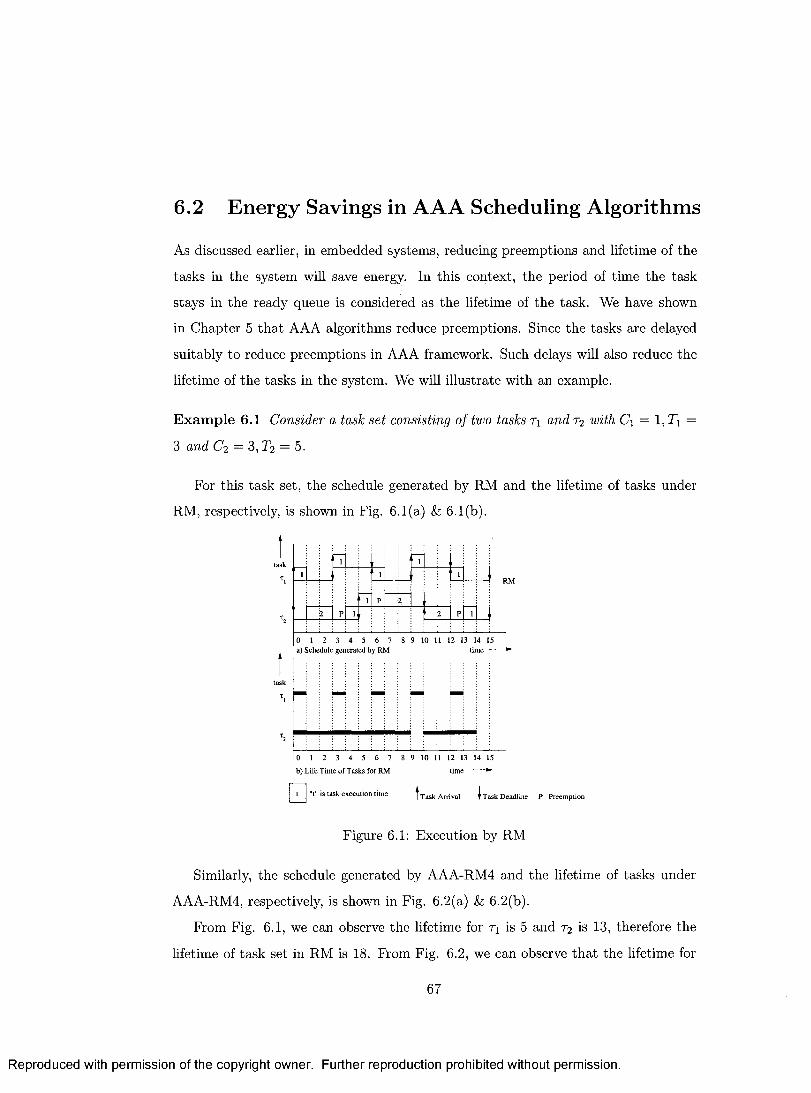
6.2 Energy Savings in A A A Scheduling A lgorithm s

As discussed earlier, in embedded systems, reducing preemptions and lifetime of the

tasks in the system will save energy. In this context, the period of time the task

stays in the ready queue is considered as the lifetime of the task. We have shown

in Chapter 5 tha t AAA algorithms reduce preemptions. Since the tasks are delayed

suitably to reduce preemptions in AAA framework. Such delays will also reduce the

lifetime of the tasks in the system. We will illustrate with an example.

Exam ple 6.1 Consider a task set consisting of two tasks T\ and r2 with C\ = 1, Tf =

3 and C2 = 3, T2 = 5.

For this task set, the schedule generated by RM and the lifetime of tasks under

RM, respectively, is shown in Fig. 6.1(a) 6.1(b).

'IL

au0 1 2 3 4 5 6 7 8 9 10 11 12 13 14 15a) Schedule generated by RM tim e —

0 1 2 3 4 5 6 7

b) L ife Tim e o f Tasks fo r RM

9 10 11 12 13 14 15

tim e -------

□ t" is task execution time t Tas t Task D eadline P Preemption

Figure 6.1: Execution by RM

Similarly, the schedule generated by AAA-RM4 and the lifetime of tasks under

AAA-RM4, respectively, is shown in Fig. 6.2(a) & 6.2(b).

From Fig. 6.1, we can observe the lifetime for Ti is 5 and r2 is 13, therefore the

lifetime of task set in RM is 18. From Fig. 6.2, we can observe that the lifetime for

67


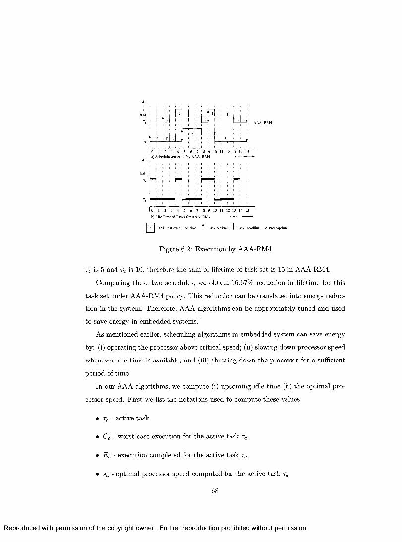
B EB EBB .

0 1 2 3 4 5 6 7 8 9 10 11 12 13 14 15a) Schedule generated by A A A -R M 4 t im e --------

0 1 2 3 4 5 6 7 8 9 10 11 12 13 14 15

b) L ife T im e of Tasks for A A A -R M 4 tim e ■

□ "t" is task execution time I TasTask A rrival t T ask Deadline P Preemption

Figure 6.2: Execution by AAA-RM4

T\ is 5 and 7 2 is 10, therefore the sum of lifetime of task set is 15 in AAA-RM4.

Comparing these two schedules, we obtain 16.67% reduction in lifetime for this

task set under AAA-RM4 policy. This reduction can be translated into energy reduc

tion in the system. Therefore, AAA algorithms can be appropriately tuned and used

to save energy in embedded systems.

As mentioned earlier, scheduling algorithms in embedded system can save energy

by: (i) operating the processor above critical speed; (ii) slowing down processor speed

whenever idle time is available; and (iii) shutting down the processor for a sufficient

period of time.

In our AAA algorithms, we compute (i) upcoming idle time (ii) the optimal pro

cessor speed. First we list the notations used to compute these values.

• Ta - active task

• Ca - worst case execution for the active task ra

• Ea - execution completed for the active task ra

• sa - optimal processor speed computed for the active task ra

68


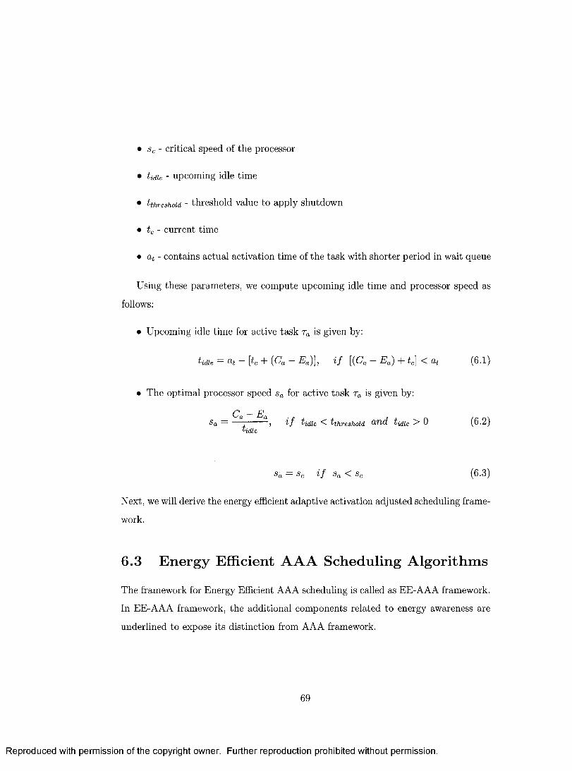
• sc - critical speed of the processor

• Udie - upcoming idle time

• tthreshold - threshold value to apply shutdown

• t c - current time

• at - contains actual activation time of the task with shorter period in wait queue

Using these parameters, we compute upcoming idle time and processor speed as

follows:

• Upcoming idle time for active task ra is given by:

Next, we will derive the energy efficient adaptive activation adjusted scheduling frame

work.

6.3 Energy Efficient A A A Scheduling A lgorithm s

The framework for Energy Efficient AAA scheduling is called as EE-AAA framework.

In EE-AAA framework, the additional components related to energy awareness are

underlined to expose its distinction from AAA framework.

tidie = at - [tc + {Ca - Ea)}, i f [{Ca — Ea) + tc\ < at (6.1)

• The optimal processor speed sa for active task ra is given by:

i f i'idle ^ t th resh o ld (d>Tld t id ie > 0 (6 .2 )

•Sa i f Sa < Sc (6.3)

69


6.3 .1 Fram ework

We consider the energy efficient Adaptive A ctivation-A djusted Scheduling

{E E — A A A ) as a quadruple < T, / a t , AT, S'" >, where


f at ■ a function defined as follows. / a t (T) = n , where II is a subset of T for which


A T : a set of pairs {Nati, ai)i), where Na>i is the next activation time and a^i is

the offset of activation adjustment of r,:. For every task r, € II, the absolute

activation time a^k is computed as stated in Chapter 5.

S'" : the scheduler. The scheduler component is a 6 tuple < Wq, Rq, Ap, s, sa, S'p >,

where


activation time.

Rq : a queue of ready tasks, ordered by decreasing priority.

Ap : a policy to select an eligible task from Wq to transfer to Rq. It returns

either the id of first eligible task or the id of a task which will become

eligible in the nearest future.

s : maximum speed of the processor.

sa : adjusted speed for the task ra.

S'” : the scheduling policy. The scheduler can be invoked either by the com

pletion of a task or by a timer expiry. When the scheduler S'" is invoked,

then

1. I f the invocation of S'" was by the completion of a task rc, then

* S'" places the completed task rc in Wq, with next adjusted activa

tion time set and updates At .

70


2. Else, I f the invocation of S'" was by timer interrupt, then

* I f a running task is interrupted by the timer, then S'" places the

interrupted task in R q.

3. S'" checks Wq to see if any tasks are to be transferred from Wq to R q

and then transfers such tasks to R q.

4. I f Rq is not empty, then

* Let ra be the task in the head of Rq, with priority p. S'" scans Wq

starting from the head and identifies the first task, say Tk , with


* S'" sets the timer to Tk ’s next adjusted activation time.

* S'" computes idle time tidie for the task ra using the equation 6.1.

* I f tjdie > 0

• S'" computes speed sa for the task ra using the equation the 6.2

and 6.3 and S'" schedules r0 with sa.

* Else,

■ S'" schedules ra with maximum speed s.

5. Else

* S'" calls Ap, and let Ap returns rk and t be the current time.

* I f Na>k - akji > t, then

• S'" transfers Tk from Wq to R q.

• go to step 3.

* Else,

■ S'" sets the timer to m inltim er, Na<k — ak,i).

• Enter processor shutdown mode if the idle time is greater than

^threshold •

6. S'" waits for its invocation.

71


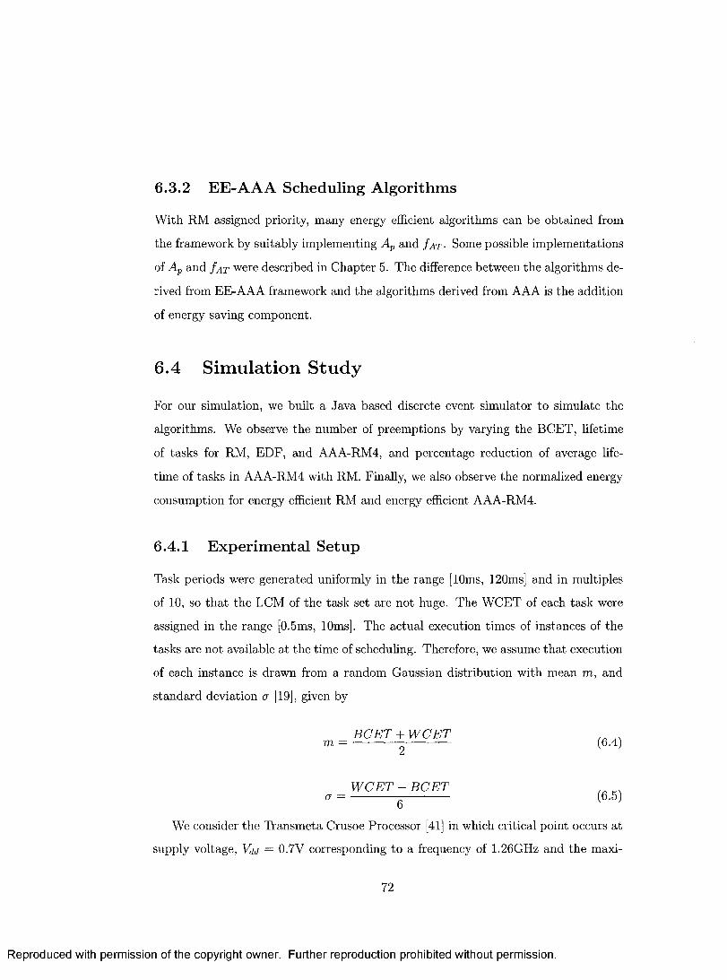
6.3 .2 E E -A A A Scheduling A lgorith m s

With RM assigned priority, many energy efficient algorithms can be obtained from

the framework by suitably implementing Ap and / at ■ Some possible implementations

of Ap and f at were described in Chapter 5. The difference between the algorithms de

rived from EE-AAA framework and the algorithms derived from AAA is the addition

of energy saving component.


For our simulation, we built a Java based discrete event simulator to simulate the

algorithms. We observe the number of preemptions by varying the BCET, lifetime

of tasks for RM, EDF, and AAA-RM4, and percentage reduction of average life

time of tasks in AAA-RM4 with RM. Finally, we also observe the normalized energy

consumption for energy efficient RM and energy efficient AAA-RM4.

6.4.1 E xp erim enta l Setup

Task periods were generated uniformly in the range [10ms, 120ms] and in multiples

of 10, so that the LCM of the task set are not huge. The WCET of each task were

assigned in the range [0.5ms, 10ms], The actual execution times of instances of the

tasks are not available at the time of scheduling. Therefore, we assume tha t execution

of each instance is drawn from a random Gaussian distribution with mean m, and

standard deviation a [19], given by

B C E T + W C E T . .m = ----------- (6.4)

W C E T - B C E T , .a = ----------- (6.5)

We consider the Transmeta Crusoe Processor [41] in which critical point occurs at

supply voltage, Vdd = 0.7V corresponding to a frequency of 1.26GHz and the maxi-

72


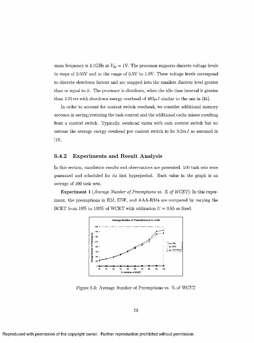
mum frequency is 3.1GHz at Vd() = IV. The processor supports discrete voltage levels

in steps of 0.05V and in the range of 0.5V to 1.0V. These voltage levels correspond

to discrete slowdown factors and are mapped into the smallest discrete level greater

than or equal to it. The processor is shutdown, when the idle time interval is greater

than 2.01ms with shutdown energy overhead of 483fxJ similar to the one in [41].

In order to account for context switch overhead, we consider additional memory

accesses in saving/restoring the task context and the additional cache misses resulting

from a context switch. Typically, overhead varies with each context switch but we

assume the average energy overhead per context switch to be 0.2m J as assumed in

[19].

6.4 .2 E xp erim en ts and R esu lt A n alysis

In this section, simulation results and observations are presented. 100 task sets were

generated and scheduled for its first hyperperiod. Each value in the graph is an

average of 100 task sets.

E x p erim en t 1 (Average Number of Preemptions vs. % of WCET): In this exper

iment, the preemptions in RM, EDF, and AAA-RM4 are compared by varying the

BCET from 10% to 100% of WCET with utilization U = 0.85 as fixed.

Average Number of Preemptions at U s 0.85

Figure 6.3: Average Number of Preemptions vs. % of WCET

73


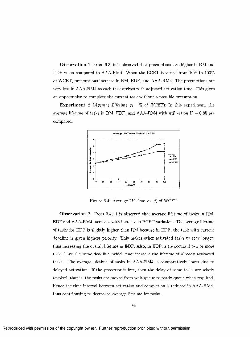
O bserva tion 1: Prom 6.3, it is observed that preemptions are higher in RM and

EDF when compared to AAA-RM4. When the BCET is varied from 10% to 100%

of WCET, preemptions increase in RM, EDF, and AAA-RM4. The preemptions are

very less in AAA-RM4 as each task arrives with adjusted activation time. This gives

an opportunity to complete the current task without a possible preemption.

E x p erim en t 2 (Average Lifetime vs. % of WCET): In this experiment, the

average lifetime of tasks in RM, EDF, and AAA-RM4 with utilization U = 0.85 are

compared.

Average Life Time of Tasks at U * 0.85

•••••■— EDF

% of WCET

Figure 6.4: Average Lifetime vs. % of WCET

O bserva tion 2: From 6.4, it is observed that average lifetime of tasks in RM,

EDF and AAA-RM4 increases with increase in BCET variation. The average lifetime

of tasks for EDF is slightly higher than RM because in EDF, the task with current

deadline is given highest priority. This makes other activated tasks to stay longer,

thus increasing the overall lifetime in EDF. Also, in EDF, a tie occurs if two or more

ta s k s h a v e th e s a m e d e a d lin e , w h ic h m a y in c re a se th e life tim e o f a l re a d y a c t iv a te d

tasks. The average lifetime of tasks in AAA-RM4 is comparatively lower due to

delayed activation. If the processor is free, then the delay of some tasks are wisely

revoked, that is, the tasks are moved from wait queue to ready queue when required.

Hence the time interval between activation and completion is reduced in AAA-RM4,

thus contributing to decreased average lifetime for tasks.

74


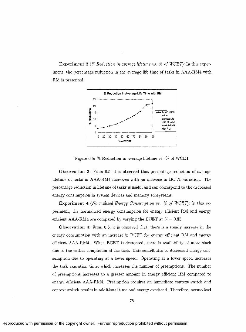
E x p erim en t 3 (% Reduction in average lifetime vs. % of WCET): In this exper

iment, the percentage reduction in the average life time of tasks in AAA-RM4 with

RM is presented.

% Reduction in A verage Life Time with RM

- ¥ - % reduction in thea v e rag e life time of task s in AAA-RM4 with RM

10 20 30 40 50 60 70 80 90 100

% o f WCET

20 -

coo3

•o4)tc$

Figure 6.5: % Reduction in average lifetime vs. % of WCET

O bserva tion 3: From 6.5, it is observed that percentage reduction of average

lifetime of tasks in AAA-RM4 increases with an increase in BCET variation. The

percentage reduction in lifetime of tasks is useful and can correspond to the decreased

energy consumption in system devices and memory subsystems.

E x p erim en t 4 (Normalized Energy Consumption vs. % of WCET): In this ex

periment, the normalized energy consumption for energy efficient RM and energy

efficient AAA-RM4 are compared by varying the BCET at U = 0.85.

O bservation 4: From 6.6, it is observed that, there is a steady increase in the

energy consumption with an increase in BCET for energy efficient RM and energy

efficient AAA-RM4. When BCET is decreased, there is availability of more slack

d u e to th e e a r lie r c o m p le t io n of th e ta s k . T h is c o n tr ib u te s to d e c re a s e d e n e rg y c o n

sumption due to operating at a lower speed. Operating at a lower speed increases

the task execution time, which increases the number of preemptions. The number

of preemptions increases to a greater amount in energy efficient RM compared to

energy efficient AAA-RM4. Preemption requires an immediate context switch and

context switch results in additional time and energy overhead. Therefore, normalized

75


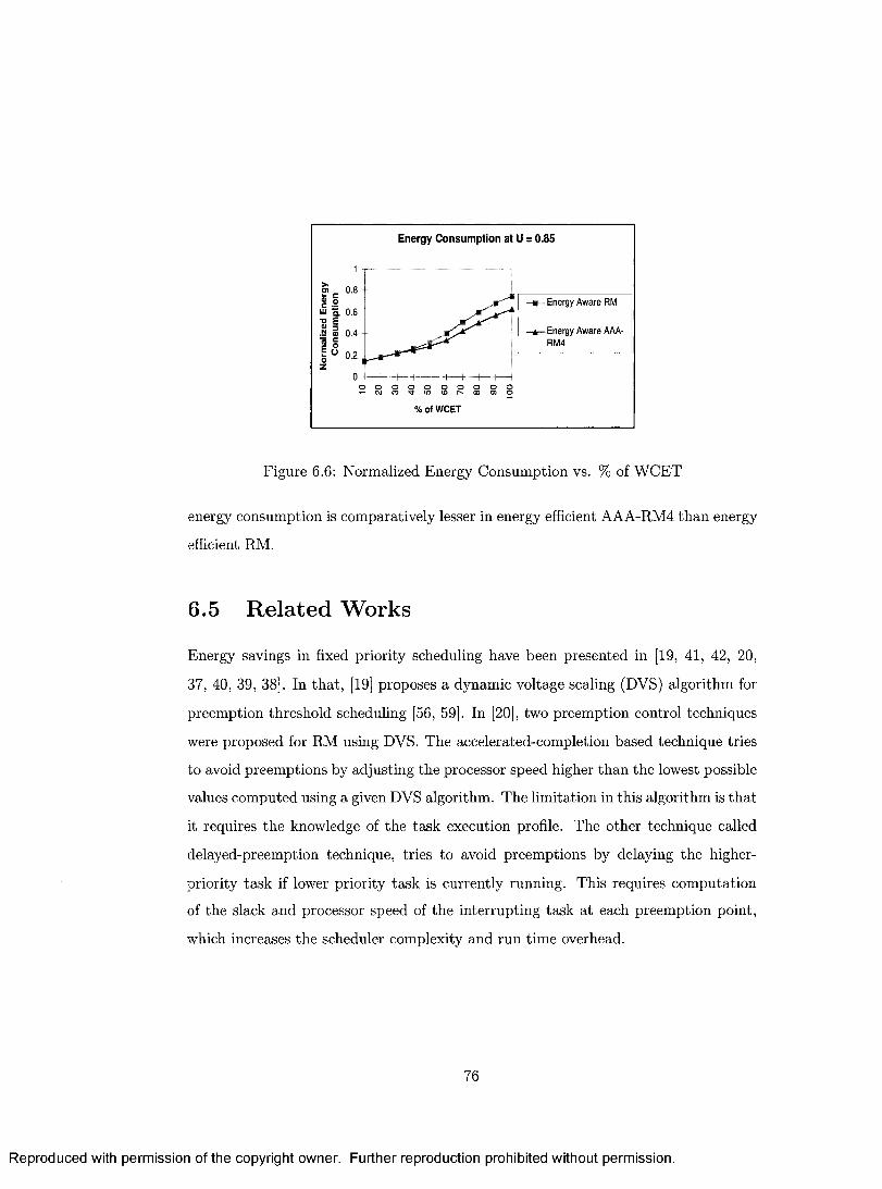
Energy Consum ption at U = 0.85

Energy Aware RM

Energy Aware AAA- RM4

0.4

0.2 - -

% o l W CET

Figure 6.6: Normalized Energy Consumption vs. % of WCET

energy consumption is comparatively lesser in energy efficient AAA-RM4 than energy

efficient RM.

6.5 R elated Works

Energy savings in fixed priority scheduling have been presented in [19, 41, 42, 20,

37, 40, 39, 38]. In that, [19] proposes a dynamic voltage scaling (DVS) algorithm for

preemption threshold scheduling [56, 59]. In [20], two preemption control techniques

were proposed for RM using DVS. The accelerated-completion based technique tries

to avoid preemptions by adjusting the processor speed higher than the lowest possible

values computed using a given DVS algorithm. The limitation in this algorithm is that

it requires the knowledge of the task execution profile. The other technique called

delayed-preemption technique, tries to avoid preemptions by delaying the higher-

priority task if lower priority task is currently running. This requires computation

of the slack and processor speed of the interrupting task at each preemption point,

which increases the scheduler complexity and run time overhead.

76


6.6 Sum mary

Preemptions and increased lifetime of the tasks are two energy consuming factors. In

this Chapter, we presented a simple class of energy efficient scheduling algorithms for

embedded systems. We conducted a simulation study for a selected algorithm and the

results show that our algorithm experiences significantly less number of preemptions

and reduces the average lifetime of the tasks, thereby reducing energy consumption.

77


Chapter 7

Conclusion and Future Directions

This thesis contains three main contributions: (i) a class of fair scheduling algorithms

for general purpose computing system; (ii) a class of efficient scheduling algorithms

for hard real-time system; and (iii) energy efficient algorithms for embedded system.

In Chapter 4, we presented a generic framework for a class of scheduling algorithms

called as Fair-Share Round Robin (FSRR) scheduling algorithms for general purpose

computing system. Then we derived a set of FSRR algorithms from this framework.

These algorithms are designed to alleviate the unfairness noticed in the traditional

round robin scheduling in treating CPU-bound and I/O-bound processes. From sim

ulation experiments, we have observed tha t FSRR algorithms have less variance in

average CPU response and average turn-around times. Therefore, the algorithms de

rived from this framework can be used in systems with varying fairness requirements

based on the implementation of the abstract components.

In Chapter 5, we introduced two frameworks, Offline Activation Adjusted Schedul

ing (OAA) and Adaptive Activation Adjusted Scheduling (AAA) for real-time sys

tems. Many algorithms can be derived from these frameworks with varying charac

teristics. Although Rate Monotonic (RM) has been widely used in practice due to its

many attractive properties, its runtime overhead has been observed as a limitation

in [13]. Many algorithms derived from our frameworks alleviate this limitation while

retaining the simplicity of the original algorithm. We conducted a simulation study

78


on the variations of RM derived from our frameworks and the results indicate that

our algorithms reduce preemptions significantly.

Due to the extensive use of embedded systems like mp3 players, cellular phones,

digital camcorders etc., minimizing the energy consumption is important in addition

to meeting the deadlines. Task preemption and increased life time are the activities

that will lead to increased energy consumption. We proposed an Energy Efficient

Scheduling (EA-AAA) by tuning AAA framework in Chapter 6. The algorithms de

rived from EE-AAA framework minimize energy consumption in embedded systems.

7.1 Future D irections

There are many directions in which the work presented in this thesis can be expanded.

Some of the directions are:

• More performance analysis of the algorithms derived from our frameworks can

be carried out to expose their properties;

• Schedulability analysis and other theoretical analysis of the algorithms derived

from our frameworks can be explored; and

• Extending the algorithms for multiprocessor systems.

79


Bibliography

[1] W. Stallings, Operating Systems: Internals and Design Principles, Fifth Edition,

Prentice Hall, 2004.

[2] H.M. Dietel, P.J Deitel, and D.R. Choffnes, Operating System, Third Edition

Pearson/Prentice Hall, 2004.

[3] A.S. Tanenbaum, Modern Operating Systems, Second Edition, Prentice Hall, 2001.

[4] A. Silberchatz and P. Galvin, Operating System Concepts, Fifth Edition, John

Wiley & Sons, 1999.

[5] J. Guynes, Impact of System Response Time on State Anxiety, Communications

of the ACM, 31 (3):342-347, 1988.

[6] B. Shneiderman, Response Time and Display Rate in Human Performance with

Computers, ACM Computing Surveys, 16(3):265-285, 1984.

[7] I. M. Flynn and A.M. McHoes, Understanding Operating Systems, Third Edition,

Brooks/Cole, Thomson Learning, 2000.

[8] C . L. L iu a n d J . W . L a y la n d , S c h e d u lin g A lg o r ith m s fo r M u lt ip ro g ra m m in g in a

Hard Real-Time Environment, Journal of the ACM, 20(1):46-61, 1973.

[9] K. Jeffay and D. L. Stone, Accounting for Interrupt Handling Costs in Dynamic

Priority Task Systems, Proc. of the I f t h IEEE-Real Time Systems Symposium,

212-221, 1993.

80


[10] J. Jonsson, H. Lonn, and K. G. Shin, Non-Preemptive Scheduling of Real-Time

Threads on Multi-Level-Context Architectures, Proc. of the IEEE Workshop on

Parallel and Distributed Real-Time Systems, LNCS, 1586:363-374, 1998.

[11] R. Dobrin and G. Fohler, Reducing the Number of Preemptions in Fixed Priority

Scheduling, Proc. of the Euromicro Conference on Real-Time Systems, 144-152,

2004.

[12] J. Lehoczky, L. Sha, and Y. Ding, The Rate Monotonic Scheduling Algorithm:

Exact Characterization and Average Case Behavior, Proc. of the IEEE Real-Time

Systems Symposium, 166-171, 1989.

[13] G. C. Buttazzo, Rate Monotonic vs. EDF: Judgment Day, Real-Time Systems,

29:5-26, 2005.

[14] M. A. Rivas and M. G. Harbour, POSIX-compatible application defined schedul

ing in MaRTE OS, Proc. of the Euromicro Conference on Real-Time Systems, 2001.

[15] J. C. Mogul and A. Borg, The effect of context switches on cache performance,

Proc. of the fourth international conference on Architectural support for program

ming languages and operating systems, 75-84, 1991.

[16] C.-G. Lee, J. Hahn, Y.-M. Seo, S. L. Min, R. Ha, S. Hong, C. Y. Park, M. Lee,

and C. S. Kim, Analysis of Cache-Related Preemption Delay in Fixed-Priority

Preemptive Scheduling, IEEE Transactions on Computers, 47(6):700-713, 1998.

[17] S. Lee, S.L. Min, C.S. Kim, C.G. Lee, and M. Lee, Cache-Conscious Limited

Preemptive Scheduling, Real-Time Systems, 17(2/3):257-282, November 1999.

[18] C.-G. Lee, J. Hahn, Y.-M. Seo, S. L. Min, R. Ha, S. Hong, C. Y. Park, M. Lee,

and C. S. Kim, Bounding Cache-Related Preemption Delay for Real-Time Systems,

IEEE Transactions on Computers, 27(9):805-826, 2001.

[19] R. Jejurikar and R. Gupta, Integrating Preemption Threshold Scheduling and

Dynamic Voltage Scaling for Energy Efficient Real-Time Systems, Proc. of the

81


Intl. Conference on Real-Time and Embedded Computing Systems and Applications,

August 2004.

[20] W. Kim, J. Kim, and S. L. Min, Preemption-Aware Dynamic Voltage Scaling

in Hard Real-Time Systems, Proc. of the ACM /IEEE Symposium on Low Power

Electronics and Design, 393-398, 2004.

[21] http://www.opengroup.Org/onlinepubs/007908799/xsh/sched.h.html, Last Ac

cessed December 21, 2006.

[22] J.A. Stankovic and K.Ramamritham, W hat is Predictability for Real-Time Sys

tems? Real-Time Systems, 2, 247-254, 1990.

[23] K.M. Zuberi, P. Pillai, and K.G. Shin, EMERALDS: a small-memory real-time

microkernel, IEEE Transactions on Software Engineering, 27(10):909-928, 2001.

[24] M. L. Dertouzos, Control Robotics: the Procedural Control of Physical Pro

cesses, Information Processes 74, 1973.

[25] H. Chetto and M. Chetto, Some Results of the Earliest Deadline Scheduling

Algorithm, IEEE Transactions on Software Engineering, 15(10):1261-1269, 1989.

[26] N. Audsley, Deadline Monotonic Scheduling, Department of Computer Science,

University of York, October 1990.

[27] J. P. Lehoczky and S. R. Thuel, An Optimal Algorithm for Scheduling Soft-

Periodic Tasks in Fixed-Priority Preemptive Systems, Proc. of the Real-Time Sys

tems Symposium, 1992.

[28] R. Davis and A. Wellings, Dual Priority Scheduling, Proc. of IEEE Real-Time

Systems Symposium, 100-109, 1995.

[29] S. Heun Oh and S. Min Yang, A Modified Least Laxity-First Scheduling Algo

rithm for Real-Time Tasks, Proc. of the 5th International Conference on Real-Time

Computing Systems and Applications 1998.

82


http://www.opengroup.Org/onlinepubs/007908799/xsh/sched.h.html

[30] L. Sha, T. Abdelzaher, K. E. Arzen, A. Cervin, T. Baker, A. Burns, G. Buttazzo,

M. Caccamo, J. Lehoczky, A. K. Mok, Real Time Scheduling Theory: A Historical

Perspective, Real-Time Systems, 28:101-155, 2004.

[31] A. Burns, K. Tindell, and A. Wellings, Effective Analysis for Engineering Real-

Time Fixed Priority Schedulers, IEEE Transactions on Software Engineering,

21(5):475-480, 1995.

[32] E. Bini, G. C. Buttazo, G. M. Buttazzo, Rate Monotonic Analysis: The Hyper

bolic Bound, IEEE Transactions on Computers, 52(7):933-942, 2003.

[33] E.Bini and G.C Buttazo, Schedulability Analysis of Periodic Fixed Priority Sys

tems, IEEE Transactions on Computers, 53(11):1462-1473, 2004.

[34] A. K. Mok, Fundamental Design Problems of Distributed Systems for the Hard-

Real-Time Environment, Ph.D. Thesis, MIT, 1983.

[35] M.B. Jones, Joseph S. Barrera III, A. Form, P.J. Leach, D. Rosu, and M.C.

Rosu, An Overview of the Rialto Real-Time Architecture, Proc. of the Seventh

ACM SIGOPS European Workshop, Ireland, 249-256, September 1996.

[36] Y. Shin and K. Choi, Power Conscious Fixed Priority Scheduling for Hard Real-

Time Systems, Proc. of the Design Automation Conference, 134-139, 1999.

[37] W. Kim, J. Kim, and S.L. Min, Dynamic Voltage Scaling Algorithm for Fixed-

Priority Real-Time Systems using Work-Demand Analysis, Proc. of the 2003 In

ternational Symposium on Low Power Electronics and Design, August 2003.

[38] Pillai and K. G. Shin, Real - Time Dynamic Voltage Scaling for Low-Power

Embedded Operating Systems, Proc. of the 18th Symposium on Operating Systems

Principles, 2001.

[39] G. Quan and X. Sharon Hu, Minimum Energy Fixed - Priority Scheduling for

Variable Voltage Processors, Proc. of the 2002 Design, Automation and Test in

Europe Conference and Exhibition, 2002.

83


[40] Y. H. Lee, K.P. Reddy, and C.M. Krishna, Scheduling Techniques for Reducing

Leakage Power in Hard Real-Time Systems, Proc. of the 15th Euromicro conference

on Real-Time Systems, 2003.

[41] R. Jejurikar and R. Gupta, Procrastination Scheduling in Fixed Priority Real-

Time Systems, Proc. of the Language Compilers and Tools for Embedded Systems,

June 2004.

[42] R. Jejurikar and R. Gupta, Dynamic Voltage Scaling for Systemwide Energy

Minimization in Real-Time Embedded Systems, Proc. of the 2004 International

Symposium on Low Power Electronics and Design, August 2004.

[43] R. Jejurikar and R. Gupta, Energy-Aware Task Scheduling with Task Synchro

nization for Embedded Real Time Systems, Proceedings of the 2002 international

conference on compilers, architecture, and synthesis for embedded systems October

811, 2002.

[44] E.G. Coffman, R.R. Muntz, and H. Trotter, Waiting Time Distributions for

Processor-Sharing Systems, Journal of the Association for Computing Machinery,

17(1): 123-130, 1978.

[45] E.G. Coffman and L. Kleinrock, Computer Scheduling Methods and Their

Counter Measures, Proc. of the Spring Joint Computer Conference, 32:11-21, 1968.

[46] L. Kleinrock, A Continuum of Time-sharing Scheduling Algorithms, Proc. of the

Spring Joint Computer Conference, 453-458, 1970.

[47] S. Haider and D.K. Subramanian, Fairness in Processor Scheduling In Time

Sharing Systems, Operating Systems Review, 25(1):4-16, 1991.

[48] J. Kay and P. Lauder, A Fair Share Scheduler, Communication of the ACM,

31(l):44-55, 1988.

[49] L. Bic and A. Shaw, Operating Systems Principles, Pearson/Prentice Hall, 2003.

84


[50] A. Silberchatz, P. Galvin, and G. Gagne, Applied Operating System Concepts,

Fifth Edition, John Wiley & Sons, 2000.

[51] W.S. Davis and T.M. Rajkumar, Operating Systems: A Systemic View, Sixth

Edition, Addison Wesley, 2004.

[52] M. Ruschitzka and R.S. Fabry, A Unifying Approach to Scheduling, Communi

cation of the ACM , 20(7):469-477, 1977.

[53] D. I. Katcher, H. Arakawa, and J. K. Strosnider, Engineering and Analysis of

Fixed Priority Schedulers, IEEE Transactions on Software Engineering, 19(9):920-

934, 1993.

[54] N. Audsley, A. Burns, M. Richardson, K. Tindell, and A. J. Wellings, Apply

ing New Scheduling Theory to Static Priority Pre-emptive scheduling, Software

Engineering Journal, 284-292, 1993.

[55] M. Naghibzadeh, K. H. Kim, A Modified Version of Rate-Monotonic Scheduling

Algorithm and its Efficiency Assessment, Proc. of the Seventh IEEE International

Workshop on Object-Oriented Real-Time Dependent Systems, 289-294, 2002.

[56] M. Saksena and Y. Wang, Scheduling Fixed-Priority Tasks with Preemption

Threshold, Proc. of the IEEE Real-Time Computing Systems and Applications,

328-335, 1999.

[57] S. Kim, S. Hong, and T.-H. Kim, Integrating Real-Time Synchronization

Schemes into Preemption Threshold Scheduling, Proc. of the 5th IEEE Intl. Symp.

on Object-Oriented Real-Tim.e Distributed Computing, 2002.

[58] S. Kim, S. Hong, and T.-H. Kim, Perfecting Preemption Threshold Scheduling

for Object-Oriented Real-Time System Design: From the Perspective of Real-Time

Synchronization, Proc. of the Languages, Compilers, and Tools for Embedded Sys

tems, 2002.

85


[59] M. Saksena and Y. Wang, Scalable Real-Time System Design Using Preemption

Thresholds, Proc. of the IEEE Real-Time Systems Symposium, 25-26, 2000.

86


Fair And Efficient CPU Scheduling Algorithms Jeyaprakash ...

Documents

Transcript of Fair And Efficient CPU Scheduling Algorithms Jeyaprakash ...