.

FAIR AND ECONOMICALLY SUSTAINABLE CHARGES FOR

THE USE OF MOTORWAY INFRASTRUCTURE

Claus Doll

Institut für Wirtschaftspolitik und Wirtschaftsforschung

6.10.2003

Keywords: Cost Allocation, Charges, Motorway Infrastructure, Game

Theory

JEL-Classification: e.g. C7, H2, H4, M4, R4

Contact Details: Institut für Wirtschaftspolitik und Wirtschaftsforschung (IWW) Universität Karlsruhe (TH) Kollegium am Schloss, Bau IV Tel: +49 (0)721 608-6042 Fax: +49 (0)721 607376 E-mail: doll@iww.uni-karlsruhe.de

1

FAIR AND ECONOMICALLY SUSTAINABLE CHARGES FOR THE USE

OF MOTORWAY INFRASTRUCTURE

Abstract:

Recent studies in different countries have shown, that there is no

agreement on a common procedure for a fair allocation of infrastructure

costs. Thus, this paper follows the goal of advancing the discussion on the

allocation of joint costs. We consider the case of road capital and running

costs or German motorways, for which a sophisticated cost model had

recently been developed and applied for estimating HGV toll levels. The

cost model ensures the sustainability of road user charges by considering

the full economic costs of providing, maintaining and operating the

infrastructure, rather than considering short-run variable or marginal

costs.

2

1 Aim and Structure of the Paper

In this paper the goal of advancing the discussion on the fair allocation of

joint costs among users is followed. We consider the case of road capital

and running costs or German motorways, for which a sophisticated cost

model had recently been developed and applied for estimating HGV toll

levels. The cost model ensures the sustainability of road user charges by

considering the full economic costs of providing, maintaining and

operating the infrastructure, rather than considering short-run variable or

marginal costs.

The paper is organised as follows: Section 2 gives a very brief overview

on recent road accounting and cost allocation studies and compares their

results. Section 3 then goes into the economic theory of games and

proposes some procedures, which are applicable in the case of road cost

allocation. Section 4 discusses and describes the cost model used for the

game-theoretic concepts. The Sections 5 finally presents some results and

Section 6 gives some concluding remarks.

2 Traditional Cost Allocation Approaches

In recent years a number of governmental bodies in Europe and the

United States have published road accounting studies. Among other

goals, they follow the aim of calculating or verifying currently existing

road user charges or taxes on fuels and on motor vehicles. For Germany

the most relevant studies in this field are the report on proposed HGV

charges for the planned motorway toll system by Prognos and IWW

(University of Karlsruhe) to the Federal Ministry for Transport, Building

and Housing (BMVBW) (Rommerskirchen et al. 2002) and the study on

3

road and railway infrastructure costs by the German Institute for

Economic Research (DIW), commissioned by the German Automobile

Club (ADAC e.V.) and the Federal Agency for Freight Transport,

Logistics and Disposal (BGL e.V.) (Link et al. 2000) In Austria the

tariffs for the electronic motorway toll system from 2004 on was

determined by a study conducted for the motorway financing society

(ASFINAG (Herry et al. 2002) and in Switzerland there is an annual

update made of the Swiss road accounts by the National Statistical Office

(BFS) (Gritti and Schweizer 2001). On the European level the research

project UNITE has carried out road cost accounts using the DIW model

for 18 European countries (Link et al. 2002) and finally the Federal

Highway Cost Allocation Study 1997 carried out for the U.S. department

of Transportation, is to be mentioned. Table 1 compares the results per

vehicle kilometre found by some of these studies, although a direct

comparison is difficult due to the different classifications of motor

vehicles used in the studies.

With the exception of the U.S. Highway cost allocation study and the

reports for Austria, all of the studies mentioned above use some kind of

equivalency factor system for allocating cost. However, there are big

differences in the consideration of capacity demand by different vehicles

and by the differentiation of construction elements. In the U.S. study, for

some construction elements an incremental approach is applied, which

allocates the additional costs caused by a particular vehicle type to this

and all “more demanding” vehicles. A complete different approach is

followed by the Austrian studies, which determine cost shares by

applying regression models of construction and maintenance costs over

various indicators of vehicle movements. This “econometric approach”

4

results in relatively high cost shares, which are similar to thise found by

the DIW model.

Table 1: Results of recent road cost allocation studies

Institute Prognos DIW DIW Herry Herry

IWW (UNITE) WKR

Area / country D (BAB) D (BAB) D (BAB) AT (A+S) AT (ASFINAG)

Year 2003 1997 2005 2000 2004

Motorcycles 1,4 0,6 0,6

Passenger cars 2,1 1,2 1,3 2,8 3,1

Buses 10,0 4,3 4,5 19,2

Vans (< 3.5t) 2,2 2,3

2,6 3,7 5,6 9,0 13,7

HGV 3,5-12t, 2 axles 12,5 9,0

HGV 12-18t, 2 axles 10,7 10,3

HGV 18-28t, 3 axles 12,1 12,5 15,7 18,6

HGV > 28t, >=4 axles 12,4 28,6 31,3

Other use vehicles 3,8 7,5 7,7

All vehicles 3,4 2,3 2,7 5,7 6,2

Share of HGV-costs 45,5% 57,3% 56,8% 56,1% 57,2%

Traffic volume HGV 17,0% 14,0% 137,0% 14,4% 13,9%

Source: Figures calculated from the sources stated in the table

The values presented in Table 1 show, that up to now there is no

consensus on the correct allocation of road infrastructure costs. All

approaches, including the Austrian allocation method, contain

considerable elements of arbitrariness and thus will always be subject to

criticism and mistrust by specific stakeholder groups or lobbyists. Thus,

in the following sections we seek for more sophisticated methods of cost

sharing, which are applicable in the case of road transport.

5

3 Cost Allocation and Game Theory

3.1 Basic Concepts

As has been shown in Section 2, in the transport sector costs are

frequently allocated to vehicle types using vehicle-kilometres or axle

kilometres, weighted by some equivalence factor. This approach assumes,

that costs caused by a specific vehicle class are strictly proportional to its

annual mileage. This assumption does not hold true in the case of

infrastrucucture costs. The high share of fixed or blockwise fixed costs

and the considerable non-linearity of the road track cost function

C(Qi,Aij) (where the Qi denote the annual vehicle kilometres performed

by vehicle type i and Aij denotes characteristic j of vehicle type i) leads to

a dependency of the costs allocated to a particular vehicle class i to the

traffic volume of all other vhicle classes j=1..n. This property calls for a

more advanced coast allocation principle.

Procedures to allocate common or non-separable costs among a group of

agents can be found in cooperative game theory. The main idea of this

economic discipline is to analyse the profit potential of some agents when

they act together on the basis of binding contracts or agreements. The

achievable gains or the minimal costs of each coalition of agents (or

players) are written into the so-called “characteristic function” v(S, where

S denotes a subset of the set of all players N={i=1..n)}. Starting from the

characteristic function cooperative game theory sug-gests the following

central cost sharing procedures:

› The Core

› The Nucleolus

› The Shapley Value and

6

› Aumann-Shapley prices.

All these concepts have in common, that all costs are allocated among the

players (pareto-efficiency) and that no player will have more costs

allocated than he would have to bear when he would act on its own

(individual rationality). The latter concept constitutes of a minimum

stability of the allocation.

The Core is a concept that delivers an entire set of cost allocation vectors

that satisfy the pareto-efficiency condition and that does not allocate more

costs to any coalition S than that coalition would bear when acting alone

(X(S) <= vIS)). The core represents the most stable set of cost

allocations, but it has the disadvantage that it might either be empty or

very large. This is not satisfying for a cost allocation scheme, but

nevertheless the core concept plays an important role as it allows to judge

other allocation schemes for their stability properties.

The Nucleolus constitutes of a cost allocation vector X=x1..xn where the

least outcome of any coalition of players is maximised. The outcome (or

excess) of a coalition is defined as the dif-ference of the costs which it

would have to bear when acting on its own (v(S)) minus the sum of the

costs allocated to all members of S (X(S)). The Nucleolus is a specifically

equitable alloca-tion procedure and it is located within the core if the core

exists. The concept can easily be ap-plied to games with very many

players of a countable number of classes and is therefore appli-cable for

price setting. Formally, the Nucleolus and the least core (leave away

restriction 1) are computed by solving the following linear programme:

7

( )

( ) (( ) ( ) :and

)()(min)(')(min|)(')(::Subject to

max!)()(min

NvNXII

SXSvSXSvSXSXI

SXSv

NSNSL

NS

=

−=−≤

→−

⊆⊆

⊆

) (3.1)

with:

N: Set of all players i=1..n S: Coalition, S⊆N X(S): Costs allocated to all members of coalition S v(S): Costs jointly caused by the Members of coalition S

In Equation 3.1, side condition (I) ensures the uniqueness of the

Nucleolus by defining an unique order of the excess vector even if the

excesses of two elements are identical. Side condition (II) ensures the

desired property of pareto-efficiency, i.e. the allocation of total costs

among all players.

The Shapley value is determined by a single formula rather than by a

optimisation procedure. It can be approached by an axiomatic approach

or alternatively by probability considerations. The axiomatic approach

demands that the cost allocation vector X=x1..xn is (1) pareto-efficient,

(2) allocates equal costs to players which cause equal costs to any

coalition which they join (symmetry) and (3) that it does not matter

whether the costs are separately allocated by cost elements (where each

costs of its own characteristic function v1...vm) or whether the allocation

uses the joint characteristic function v=v1+...+vm (additivity). The

probabilistic approach defines the allocated costs as the average marginal

costs of each player i considering each coalition S and the probability of

its formation. The formula resulting from both approaches is given by

the simple expression in Equation 3.2:

8

( )

{ }( ) {}( )( )iSvSv

!N!SN!S

XiNS

i −−−−

= ∑−⊆

1

(3.2)

Aumann-Shapley prices are the result of extending the Shapley-value to

games with infinitely many players. Like this, Aumann-Shapley prices

can be approached by several ways: An axiomatic system, a probabilistic

approach (= the mixing value) and by the limit which the formula of the

Shapley value takes when N approaches infinity. All these approaches

result in a single value, which is computed by the average marginal costs

of player i concerning all levels of total demand, but a constant mix of

demand concerning all players i=1..n. In contrast to the original Shapley

value, which is very sensitive to the definition of players, Aumann-

Shapley prices re-main relatively stable to the regrouping of players or to

small changes in the characteristic function. However, as can be seen in

the following definition function, they require a at least continuous cost

functions. Fixed cost element cannot be allocated by this cost sharing

mechanism. When C(q1...qn) describes the cost function of the n types of

players, Aumann-Shapley prices are computed as follows:

( )dt

ttfp

i

ni ∫ ∂

∂=

1

0

1

µµµ K (3.3)

with:

pi: Costs allocated to a non-atomic player i f(): Cost function (characteristic function) t: Model variable µi: Total demand by player group i

These cost allocation methods and variations of them had been applied to

allocate costs in various sectors of economy - mostly to allocate

9

investment of service related costs. Littlechild and Thompson (1977)

have estimated aircraft landing fees at Birmingham airport applying the

Nucleolus and the Shapley value, Billera and Heath (1978) have

determined optimal telephone billing rates and Castarno-Pardo and

Garcia-Diaz (1995) have allocated road pavement costs using Aumann-

Shapley prices. However, to our knowledge this approach has never been

used before to allocate external costs of transport. Accordingly, the

application of these techniques to the problem of allocating the costs of

railway noise among several train classes is new and should bring some

further light into the discussion of pricing for transport externalities.

3.2 Applicability for allocating road track costs

As is argued in Section 3.1, the Core-concept is not appropriate to the

question of finding a fiar and equitable vector allocating joint costs

among various agents as it is either not unique or my by empty. The

uniqueness property is fulfilled by the Nucleolus, which is one of the core

elements in case the core is non-empty, but it is very difficult to compute

for many players. Further, one could say that the uniqueness of the

Nucleolus is arbitrarily selected as it may depend on the order numbers of

the players. Therefore, Holler and Illing (2001) have labelled the

Nucleolus a “set-concept” comparable to the Core. For these reasons we

concentrate on the Shapley-like concepts, which are the Shapley-value

and the Aumann-Shapley-solution.

For real world problems the definition of what is a player is decisive for

both, the applicability of certain concepts of game theory and for the

output of the cost allocation itself. Both can be demonstrated for the

Shapley-value. This solution concepts consists of the property to allocate

10

fixed or blockwise fixed costs equally to all players for who they occur.

This means, that the number of payers determines the share of costs borne

by each of them. If we consider now the classification of road vehicles

into two groups, e.g. passenger vehicles and lorries, each group gets

allocated 50% of the fixed costs associated with road construction. If we

now subdivide passenger vehicles into cars and buses, each group,

including the lorries, which are nto subject to a reorganisation of the

players, gets allocated only 33% of the fixed costs.

Vice versa, starting from this undesirable property we define the

consistency condition as follows: A cost allocation scheme is consistent

with respect to the grouping of players, if the allocation to a player i is not

affected by the regrouping of other players j≠j. This property should be

fulfilled by cost allocation schemes in order to obtain results, which are

robust with respect to the quality of input information. In case the goal of

cost allocation is to derive user prices the players in the game are to be

defined as the units, which are to be priced. More generally, the players

should be atomic units, which can not be further subdivided. If the game

is specified according to this principle, the Shapley-value is consistent

according to the above definition.

If we consider that, in the case of road traffic, the single units (the atomic

players) are the vehicle kilometres or vehicle movements on the

considered network section, the problem we face gets obvious: The

complexity of the Shapley-value, e.g. the number of possible coalitions to

be analysed, is 2n, (where n denotes the number of players). For each of

those coalitions, the characteristic function needs to be calculated in

average 1+n/2 times. While the problem for 10 players (=1024

coalitions), the problem s well computable even by an Microsoft Excel

11

spreadsheet model, a number of 25 players, which corresponds to the

number of vehicle groups considered by the U.S. Highway Cost

Allocation Study, yields 33’554’432 coalitions. Depending on the

complexity of the cost estimation algorithm, this dimension may already

entail considerable non-acceptable computing times.

But how to proceed with the allocation of costs at roads, which may well

have more than 50’000 vehicle passages per day (in both directions)? To

make the problem more simple, Littlechild and Thompson (1974) have

introduced the class of airport games, which are characterised by a strict

order of the users, concerning their requirements towards the construction

standard of infrastructure assets. In this case the Shapley-value coincides

with the incremental cost procedure applied by the U.S. FHCAS. Due to

the additivity property of the Shapley value this order can be different for

various parts of the infrastructure, but the class of airport games does

exclude cases, where several players demand for different dimensions of

the asset and where total costs are not simply a linear function of these

dimensions. An example can be given in the case of road transport:

Heavy axles demand for additional thickness of the different layers (in

particular of the main course), while cars due to their high traffic volume

and safety requirements determine the width of the pavement. Total costs

then are proportional to the product out of with and thickness So we can

not say that a road, which was built for trucks, is adequate for passenger

cars. Consequently, airport games are not applicable to the present case

of allocating road track costs.

Fragnelli et al. (2000) have extended the class of airport games to so-

called infrastructure games, which consist of two parts: construction

games and maintenance games. While construction games are identical

12

tot he airport games, maintenance games are described by a matrix of

additional maintenance costs, which each user group causes on a ligher-

level infrastructure. In the case of railway infrastructure cost allocation,

where this model had been applied, this makes sense as e.g. regional

trains also cause damages to high speed tracks and their specific facilities,

although they do not need them. But also here a strict order of players

concerning their cost causation is required and thus also the infrastructure

games according to Fragnelli et al. (2000) do not apply to the road case.

A pragmatic solution for making the Shapley-value computable for a big

number of players is to slightly change the number of players as follows:

First, we determine the maximum number of players to be considered. All

these players are equal in size, i.e. they consist of the same amount of

traffic volume and each player is assigned to the characteristics a specific

vehicle class. In other words, we press the original demand structure into

a grid square and consider the contents of each grid a player in the new

game. We only must ensure that each class or players is represented by at

least one element of the grid. Clearly, the presentation of the prevailing

demand structure improves with an increasing number of grid elements.

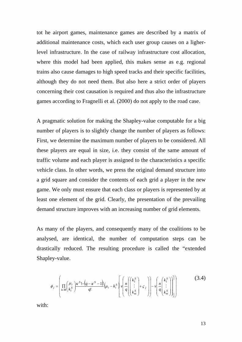
As many of the players, and consequently many of the coalitions to be

analysed, are identical, the number of computation steps can be

drastically reduced. The resulting procedure is called the “extended

Shapley-value.

( ) ( )⎟⎟⎟⎟

⎠

⎞

⎜⎜⎜⎜

⎝

⎛

⎥⎥⎥⎥

⎦

⎤

⎢⎢⎢⎢

⎣

⎡

⎟⎟⎟⎟

⎠

⎞

⎜⎜⎜⎜

⎝

⎛

⎟⎟⎟⎟

⎠

⎞

⎜⎜⎜⎜

⎝

⎛

−

⎟⎟⎟⎟

⎠

⎞

⎜⎜⎜⎜

⎝

⎛

⎟⎟⎟⎟

⎠

⎞

⎜⎜⎜⎜

⎝

⎛

+⎟⎟⎟⎟

⎠

⎞

⎜⎜⎜⎜

⎝

⎛

−−−−

⎟⎟⎠

⎞⎜⎜⎝

⎛∏=∈ S

m

S

jSm

S

Sii

SS

Si

i

Mij

k

k

qnv

k

k

qnvk

qq

kMM11

!!1! ςµκκµ

φ (3.4)

with:

13

Φj: Total amount allocated to player goup j. n: Number of players in the original game m: Number of player groups in the extended game q: Number of grid elements in the extended game M: Set of all player groups in the extended game

(M={i=1...m}) µi: Total number of grid elements allocated to player group i S: Index for a coalition of payer groups, represented by the

vector kiS

kiS: Number of grid elements of player group i in coalition S

κS: Total number of grid elements in coalition S ςj: Unity vector with ςj(j)=1 and ςj(i≠j)=0 for each i∈M

If there is no modification to the original demand structure required to fit

to the grid structure, the procedure leads to an exact computation of the

Shapley value with much less computational effort. However, concerning

usual traffic pattern on motorways we observe, that some vehicle classes

do have a share of less than 1%, while passenger cars usually constitute

of 70% to 90% of daily vehicle kilometres. On the one hand this uneven

player structure favours the application of the extended Shapley concept

as the huge players reduce the number of combinations of coalitions, as

many of them are equal. On the other hand, the good representation of

small players requires a high number of grid elements, which

exponentially increases the complexity of the procedure. Table 2 presents

the complexity issue for a very simple game structure.

Another approach towards the allocation of joint costs is the application

of the Aumann-Shapley concept. However, in its elementary definition

according to Equation 3.3 it puts some quite important restrictions on the

cost function f: First, it must be continuous across the domain of all

demand values tµ and second, f(0)=0 must be fulfilled. Together with

some other conditions game theory defines the space of functions pNA,

which must contain f. Aumann and Shapley show that only in this case

14

that their so-called “diagonal formula” leads to a solution according to

their axiomatic principles stated in section 3.1.

Table 2: Complexity of the extended Shapley procedure

Size of players i Number of grid elements q:

µ1 µ2 µ3 µ4 µ5 10 20 50 100

0,35 0,35 0,30 64 448 5.184 40.176

0,60 0,30 0,10 56 273 2.976 20.801

0,90 0,05 0,05 10 76 414 3.276

0,25 0,25 0,25 0,25 81 1.296 28.561 456.976

0,50 0,30 0,15 0,05 48 616 9.984 151.776

0,80 0,10 0,05 0,05 18 204 2.214 32.076

0,20 0,20 0,20 0,20 0,20 243 3.125 161.051 4.084.101

0,80 0,10 0,05 0,03 0,03 18 102 2.952 48.114

Original Shapley value: 1.024 1.048.576 1,13E+15 1,27E+30

Source: Own calculations

Mertens (1988a and 1988b) has proposed an extension of the diagonal

formula due to Aumann and Shapley by exchanging the order of

differentiation and integration in Equation 3.3. By this modification we

achieve that blockwise fixed costs to not matter any more. The only

remaining requirements to the cost function now is f(0)=0 and f must be

differentiable around 0 and the level of total demand µ. Both conditions

can easily be fulfilled by setting f(|µ|<k)=0 (k is a small real constant)

and by slightly in- or decreasing µ in case the second condition is

violated.

In our case the cost function is not explicitly given as a mathematical

expression and we thus deal with differential quotients rather than with

derivatives. This gives us the possibility to introduce a “smoothing

factor”, which determines the width of the differentiation interval. If we

define the minimal required width e of the differential interval as the

15

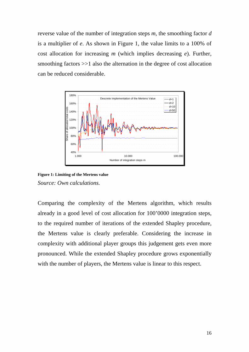
reverse value of the number of integration steps m, the smoothing factor d

is a multiplier of e. As shown in Figure 1, the value limits to a 100% of

cost allocation for increasing m (which implies decreasing e). Further,

smoothing factors >>1 also the alternation in the degree of cost allocation

can be reduced considerable.

Descrete Implementation of the Mertens Value

40%

60%

80%

100%

120%

140%

160%

180%

1.000 10.000 100.000Number of integration steps m

Shar

e of

allo

cate

d to

tal c

osts

d=1d=2d=10d=50

Figure 1: Limiting of the Mertens value

Source: Own calculations.

Comparing the complexity of the Mertens algorithm, which results

already in a good level of cost allocation for 100’0000 integration steps,

to the required number of iterations of the extended Shapley procedure,

the Mertens value is clearly preferable. Considering the increase in

complexity with additional player groups this judgement gets even more

pronounced. While the extended Shapley procedure grows exponentially

with the number of players, the Mertens value is linear to this respect.

16

4 the Cost Model

4.1 Basic concept

The cost model we use to generate the characteristic function is fairly

simple. This property is important because it has to be computed several

thousand, or even million times. The model is defined on the basis of the

cost model for the German federal road network, which was developed by

Prognos and IWW in 2002 for calculating the tariffs of the planned HGV

motorway toll (Rommerskirchen et al. 2002). However, the model used

here had to be extended and simplified in some dimensions.

It was extended to take into account the traffic volumes and the traffic

mix when designing road structures in order to give a realistic estimate of

the costs associated with each coalition of players. In this respect the

model structure is organised along the main planning and maintenance

steps of road investment procedures. On the other hand, the

Prognos/IWW model had to be simplified with respect to the

consideration of the stochastic depreciation of assets and the

consideration of road quality data. The cost function used here is a simple

time-based model of capital depreciation, which ignores the influence of

traffic loads on depreciation periods.

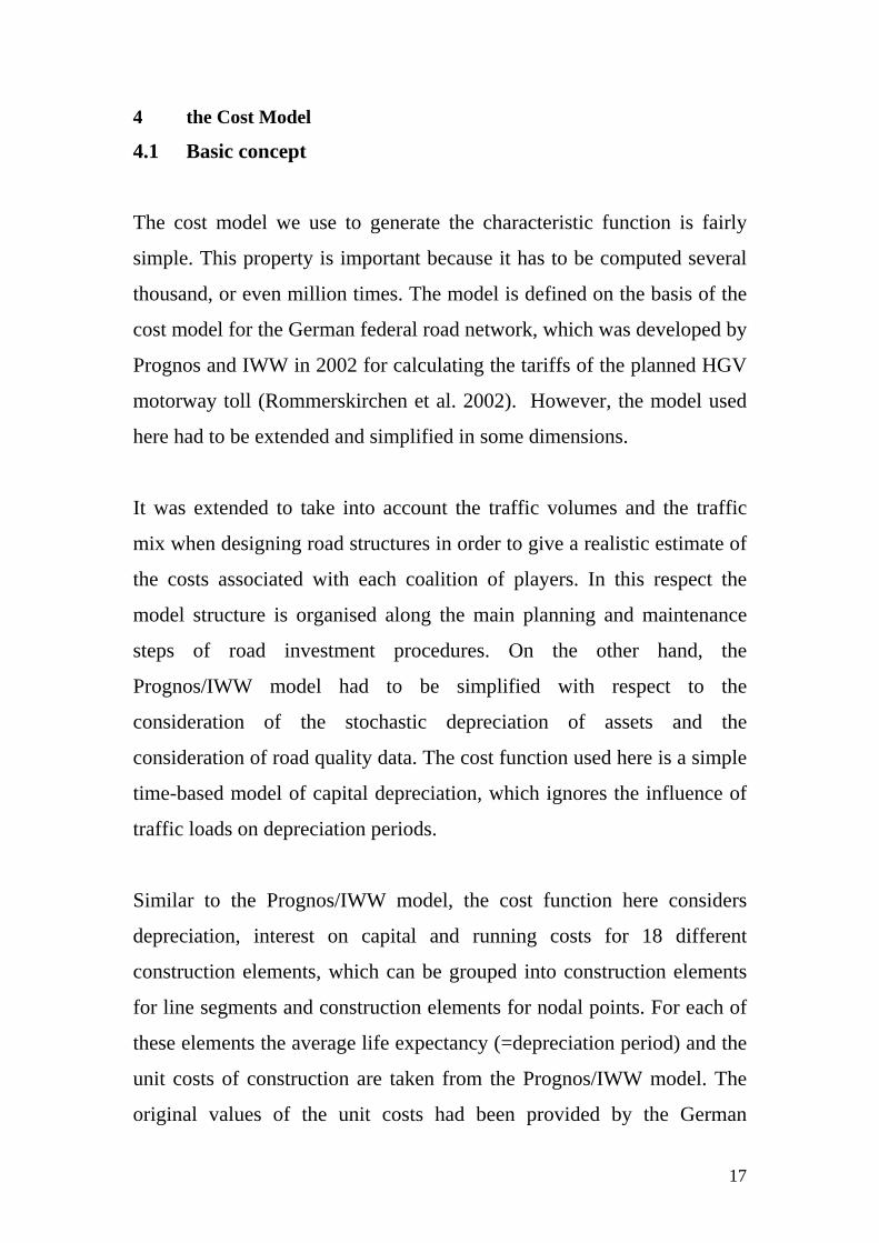
Similar to the Prognos/IWW model, the cost function here considers

depreciation, interest on capital and running costs for 18 different

construction elements, which can be grouped into construction elements

for line segments and construction elements for nodal points. For each of

these elements the average life expectancy (=depreciation period) and the

unit costs of construction are taken from the Prognos/IWW model. The

original values of the unit costs had been provided by the German

17

Ministry for Transportation, Building and Housing (MBVBW) according

to recent construction projects as well as from the forecast on

rehabilitation requirements until 2010 (Maerschalk 2001). Here, we have

averaged the values across federal states and road types in order to keep

the model simple. Further, for each construction element a set of

parameters is given, which determines the functional relationship

between traffic volume, traffic mix and the dimensioning of the element.

Table 3 presents the construction elements and their basic parameters.

Table 3: Construction elements of the cost model

Construction element Used for: Depreciation Unit replacement

Lines. Nodes period costs

Land purchase x x inf. 10,96 €/m²

Earthworks x x 90 70,84 €/m²

Frost preservation course x x 90 97,45 €/m³

Main course x x 45 97,45 €/m³

Binder Course x x 30 238,68 €/m³

Surface course x x 15 164,95 €/m³

Bridges x x 65 2181,30 €/m²

Tunnels x 90 1693,19 €/m²

Other engineering works x 50 100,00 €/m

Equipment x x 18 607,36 €/lane-m

Source: Figures based on Rommerskirchen (2002)

The basis for calculating capital costs is the estimation of gross asset

values for each of the construction elements. Gross values are calculated

by the replacement cost principle by multiplying the dimensions (m, lane-

m, m² or m³) of each construction element with the unit replacement costs

from Table 3. The dimensioning of each element is carried out separately

for each coalition considered in the cost allocation procedure. The

dimensioning process will be described in detail throughout this section.

18

When dimensioning the assets, e.g. setting their length (if not given by

the network database), width and thickness (or more generally: the

construction standard), we take the viewpoint of a traffic planner at the

period of investment or renewal. Alternatively, we could have decided to

put ourselves in the position of the decision maker at the current time

period, which would be somewhat more compatible to the concept of

replacement costs, but this approach would not be able to explain the

causation of the costs associated with the actually existing infrastructure

asset.

For the calculation of net asset values, information on the age of

earthworks, the main course, the surface course and bridges is provided

by the transport network database. The age of all assets, which are not

directly referred to in database are set according to similar construction

elements, of which data is existing. In particular it is assumed that the age

of nodal points (including intersections and exit points) equals those of

the line segments. In case the age of a particular asset exceeds its life

expectancy it is assumed that it has been re-invested meanwhile and thus

the age is reduced by the life expectancy.

The net values then are simply determined by a linear depreciation from

the investment period to the ent of the life expectancy of the construction

element. The use of variable life spans, which are depending on traffic

load, would cause problems as at a particular time period an asset might

be written down and thus would be re-invested for some coalitions, while

it would be nearly written down for others. As this could lead to paradox

effects, we have decided to keep the depreciation period of assets fix

(compare the values given in Table 3).

19

Depreciation costs than are simply determined by the quotient of the

gross capital value and the assets depreciation period. Interest costs are

determined by multiplying the net asset value with a social interest rate.

As the current model uses the replacement cost approach, and thus the

replacement cost values already contain price inflation, we have to apply

real interest values here. In accordance with Rommerskirchen (2002) we

use a rate of 3.5%.

The cost model does not yet contain a sophisticated procedure for

estimating running costs. Thus, we assume a value of 0.03 € per vehicle-

km in order to meet the total running costs reported by the Prognos/IWW

model.

4.2 Characteristics of traffic demand

The dimensions of the road elements are determined by three

characteristics of the vehicle stream, which are:

• Passenger car equivalents (PE-weighted vehicle kilometres)

• Equivalent standard axle loads (ESAL-weighted vehicle kilometres)

and

• Desired design speeds.

In the detailed annexes of the U.S. Federal Highway Cost Allocation

Study 1997 (FHWA 1997) it is reported, that passenger car equivalents of

goods are far from being a constant value. They depend on the vehicles’

geometry, on the ration between vehicle weight and horsepower, on the

gradient of the road and on traffic conditions. Out of the data found in

20

U.S. sources and in the German HBS manual on Road Design (FGSV

2001a) we have constructed a simple model of the form:

( )290.2113786.0

71.45574.0

12045.121

4000⎟⎠

⎞⎜⎝

⎛⎟⎠

⎞⎜⎝

⎛⎟⎠

⎞⎜⎝

⎛+⎟⎠⎞

⎜⎝⎛= iii

iVLG

SQPE (4.1)

with:

PEi: Passenger car equivalent of vehicle type i Q: Traffic volume in both directions; Q>4000 S: Gradient of the road segment G:i Weight / horsepower ratio of vehicle type i (Kg/kWh) L:i Length of vehicle type i (m) Vi: Usual travel speed of vehicle type i (kph)

We assume, that the decisive parameter for the design of the horizontal

road structure is the PE-weighted traffic volume in the peak hour at the

end of the life expectancy of the main course. This can be easily

calculated using vehicle demand growth rates and share of traffic in the

peak period from the vehicle database in combination with data on the

remaining life expectancy of the main course and the PE factors

according to equation 4.1.

The standard axle factor of each vehicle type is calculated according to

the scheme set out in the German RStO manual for road pavement design

(FGSV 2001b) is calculated according to the 4th power rule. We consider

the total weight of the vehicle and the load of the heaviest axle. This data

is provided by the vehicle database. Further we assume that all other

axles are loaded equally by the remaining vehicle weight. In the

preliminary version of the model we assume, that all vehicles are fully

loaded up to the total permissible gross weight. For purposes of road

thickness design the ESAL-weighted traffic volumes during the entire life

expectancy of the respective assets is required.

21

The desired design speed simply represents the highest usual travel speed

among all vehicle classes, which is given by the vehicle database.

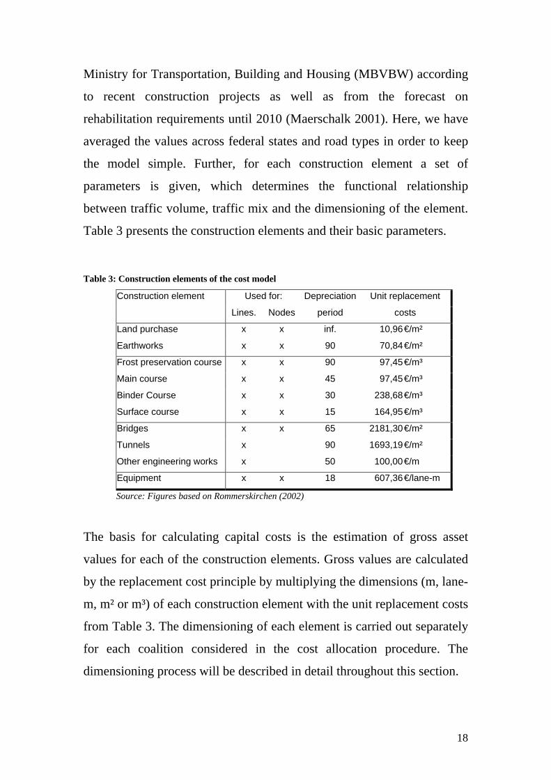
4.3 Dimensioning and Design principles

The width design of road segments distinguishes between a number of

different design elements according to the German RAS-Q manual on the

cross-sectional design of road profiles (FGSV 1996). The design elements

and their width are presented Table 4 for a number of norm profiles.

Considering the typical use of these norm profiles with respect to traffic

volume, traffic mix and functional type of the road link given in compare

FGSV 1988, we were able to create a simple design model for arbitrary

traffic demand situations, which are characterised by the variables

introduced above.

Table 4: Specification of Norm Profiles

Width Rule-

cross

section

Numbe

r of

lanes

lanes

[m]

Edge

trims

[m]

Central

reserves

[m]

Emergency

lanes

[m]

Shoulder

[m]

Separation

reserves

[m]

1 2 3 4 5 6 7 8

RQ 35,5 6 3,75 /3,50 0,75/0,50 3,50 2,50 1,50 3,00

RQ 33 6 3,50 0,50 3,00 2,00 1,50 3,00

RQ 29,5 4 3,75 0,75 3,50 2,50 1,50 3,00

RQ 26 4 3,50 0,50 3,00 2,00 1,50 3,00

RQ 20 4 3,25 0,50 2,00 - 1,50 1,75

RQ 15,5 2+1 3,75/3,25/3

,50

0,25 - - 2,50/1,50 1,75

RQ 10,5 2 3,50 0,25 - - 1,50 1,75

RQ 9,5 2 3,00 0,25 - - 1,50 1,75

RQ 7,5 2 2,75 - - 1,50 1,25

Source: FGSV 1996

22

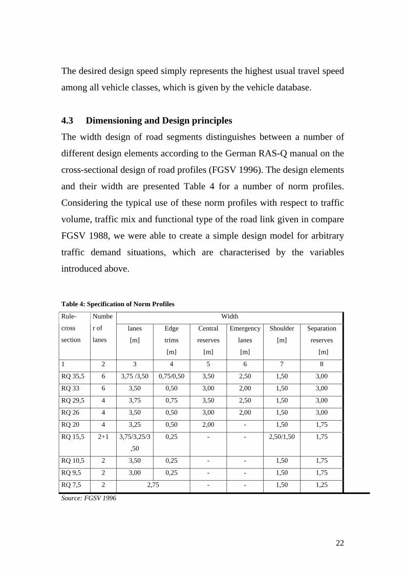
Starting from the single design elements presented in Table 4, we can

define the width of the superstructure (consisting of the frost preservation

course the main course, the binder course and the surface layer, bridges

and tunnels), substructures (additinally consisting of all non-paved

earthworks) and the total land to be purchased. Figure 2 presents the

figures retrieved for an average traffic composition of 15% heavy

vehicles and a design speed between 80 kph for low traffic volumes and

120 kph for high demand levels. Further to these default values, the

design of the single profile elements are made variable with respect to the

design speed and the vehicle geometry. Considering further the variability

of the PE factors according to Equation 4.1, we receive a rather flexible

model of structure road profile design.

Width of Structural Elements for Usual Traffic Compositions

0

10

20

30

40

50

60

70

0 10000 20000 30000 40000 50000 60000 70000 80000 90000 100000

ADT (vehicles / 24h)

Wid

th (m

)

Superstructure

Substructure

Land purchase

Validity range of the RAS-Q manual

Figure 2: Road width design for a usual composition of the traffic flow

Source: Figures from FGSV (1996)

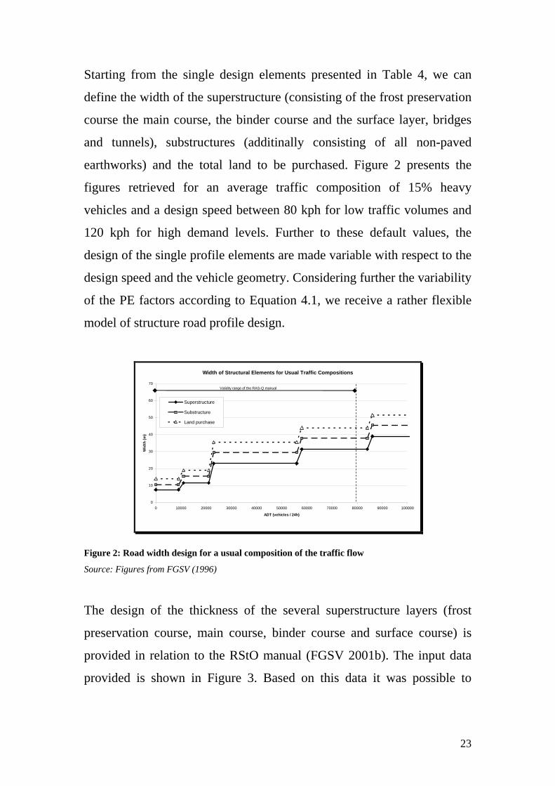
The design of the thickness of the several superstructure layers (frost

preservation course, main course, binder course and surface course) is

provided in relation to the RStO manual (FGSV 2001b). The input data

provided is shown in Figure 3. Based on this data it was possible to

23

estimate design models for each layer. The following functional form was

chosen:

jc

njjj ESALbaD += (4.1)

with:

Dj: Thickness of layer j (in m) ESALjL Standard axle loading during the depreciation period of jaj,bj,cj: Model parameters

0

5

10

15

20

25

30

35

40

321030,80,30,10Million ESAL-km

Thic

knes

s (c

m)

Surface layerBinder courseMain course

Figure 3: Thickness of superstructure layers for flexible pavements

Source: Figures from FGSV (2001b)

For other structural elements, which do not have a physical thickness, the

thickness property is used to express the influence of traffic flow or

regional parameters on purchase or construction prices.

• In this sense, the “thickness” of land purchase expresses the difference

in purchase prices per m² between different area types. For urban

areas German data provided by the Federal Statistical Office

(Statistisches Bundesamt) reveals, that land prices for transportation

infrastructure are nearly five times higher than in rural areas.

• Concerning earthworks, the parameter expresses the difficulty of

ground preparation, including the establishment of embankments and

24

drainage in relation to the terrain formation. However, this model part

is not implemented yet.

• In the case of bridges the parameter expresses the increased strength

required due to heavy axles. From German and Swiss experiences we

know that approximately 85% of bridge costs are fixed. For the

remaining 15% we use the parameters estimated for the the thickness

of the main course as other information had not been evaluated up to

now.

Besides Tunnels and other engineering works, nodal points consist of the

same construction elements than node-free road segments. In German two

manuals for the design of nodes exist: The RAS-K-1 manual for nodal

points at grade (FGSV 1988a) and the RAL-K-2 manual for grade-

separated nodes (FGSV 1976). From these manuals we retrieve the

following design principles for the length of travel lanes at nodes:

Up to a volume of turning traffic in either direction of 750 PE per hour

with a design speed of 90 kph we can apply junctions at grade. However,

this value decreases significantly when the design speed increases above

100 kph. Crossings and exit points at grade may consist of special lanes

for traffic turning left and / right. Their requirement and dimension

depends on traffic volumes and design speed.

We assume that level-free crossing consist of direct ramps for turning

right, indirect ramps for turning left and weaving lanes for traffic exiting

and entering the main travel lanes. The total length of all ramps can be

estimated as a function of the radius of the indirect ramps. This radius

varies between 25m for a design speed of 30 kph (on the ramp) and 50m

for a maximum design speed of 40 kph. By defining a simple linear

25

function, which explains the design speed in the ramp by the design speed

on the node-free road segment we finally retrieve a relationship between

the general design speed and the length of the ramps.

The width and the thickness of the ramps are defined in accordance with

the design principles for straight road segments. Specific, however, is the

determination of the land purchase, which is not simply going along the

ramps but cuvers the entire area, enclosed by the node. For level free

crossings we assume that 70% of all ramps are bridges.

There are two decisive parameters influencing the costs of nodal points:

The share of turning traffic and the average number of nodal points per

network kilometre. In the first case we estimate, that from the traffic flow

per direction of the node-free lanes 15% turn into each direction. I.e. 70%

of traffic goes straight on. The traffic mix of turning traffic is assumed to

be equal to that on the road segments. Concerning the second parameter

we estimate on the basis of data from the German federal road network,

there is a nodal point each 12 km.

5 Results

The following subsections contain some results, which demonstrate a

number of basic properties of the two cost allocation procedures which

have been identified as appropriate tools to allocate the costs of large

games with non-continuous cost functions: The extended Shapley value

and the discrete implementation of the Mertens value. To generate these

results, the following vehicle flow database is used:

26

Table 5: Average daily traffic per network kilometre

Pass. car

Mot. cycle

Bus+ coach

LDV < 3.5t

LDV > 3.5t

Oth. use v.

HGV 2 ax.

HGV 3 ax.

HGV 4 ax.

HGV 5+ ax.

22300 1357 3435 4125 385 37 166 347 666 1823

The costs are computed for a straight and flat road segment of 1 km

length with 100 m of bridges and a tunnel of 25 m length. The age of

assets is set to 50% of their life expectancy. The density of nodal points is

assumed to be one each 12 network kilometres.

5.1 Performance of the Extended Shapley Procedure

The first question we are interested in is, how the number of grid

elements, i.e. the difference between prevailing and model-internal traffic

volumes, impacts the result of the allocation process. Table 6 thus

presents total and average costs by vehicle category, which are allocated

using 30 to 90 grid elements. As expected, the costs allocated to the

vehicle categories with low traffic volumes are widely over-estimated the

smaller the number of grids is. Only for passenger cars the fluctuation of

allocated costs remains relatively stable within a range of 10%. As

average costs are derived from total costs using the adapted traffic

volumes, they deviate much less than the total cost figures. Accordingly,

we can conclude that the extended Shapley value is appropriate for

approaching tariffs, even with a relatively small number of grid elements

(The computing time of the algorithm is approximately one our per

network link using 90 grid elements, and only one minute with 60

elements).

The two right columns of Table 6 present calculations with an adapted

traffic volume configuration, which already fits into a 50-element grid.

27

This delivers an exact solution of the Shapley value and thus it allows to

compare the results of the extended Shapley algorithm to those of the

Mertens procedure. While especially for the heavy vehicles the average

cost results are surprisingly similar, considerable differences must be

constituted for passenger cars, and here in particular for motorcycles and

buses.

Table 6: Results for various grid densities of the extended Shapley procedure

Vehicle- Original traffic mix Adapted traffic mix

category Extended Shapley procedure Ext-S Mertens

Number of grid elements Grid Inter.

30 40 50 60 70 80 90 50 100000

Total allocated annual costs (Euro / road-km)

Pass. car 209,1 205,1 221,3 232,8 234,9 220,8 236,1 227,2 293,5

M.cycle 28,6 23,3 21,2 21,3 20,7 22,0 21,4 23,5 10,6

Bus+coach 32,3 44,9 52,8 50,0 44,5 49,2 46,5 38,8 59,7

LDV < 3.5t 102,9 108,2 113,4 113,8 117,1 119,8 124,4 118,0 135,2

LDV > 3.5t 68,0 53,9 43,0 38,5 34,2 30,8 28,6 47,3 13,2

Other use v. 58,9 46,9 36,6 32,9 29,0 26,1 24,2 41,0 1,2

HGV 2 ax. 105,7 87,0 69,4 60,3 54,5 49,1 45,8 74,8 9,6

HGV 3 ax. 109,1 90,0 72,1 62,5 56,6 51,1 47,8 77,6 21,2

HGV 4 ax. 132,8 106,2 84,5 74,7 67,2 60,6 56,6 91,1 48,4

HGV 5+ ax. 166,7 134,8 109,3 191,1 171,8 155,5 144,8 118,1 168,3

Allocated average costs (Euro / vehicle-km)

Pass. car 0,030 0,029 0,029 0,030 0,030 0,028 0,030 0,029 0,036

M.cycle 0,037 0,039 0,047 0,052 0,058 0,035 0,038 0,048 0,021

Bus+coach 0,042 0,038 0,039 0,041 0,041 0,039 0,041 0,040 0,048

LDV < 3.5t 0,079 0,079 0,081 0,082 0,082 0,084 0,085 0,084 0,090

LDV > 3.5t 0,088 0,091 0,095 0,094 0,095 0,099 0,101 0,098 0,094

Other use v. 0,076 0,079 0,081 0,080 0,081 0,084 0,086 0,084 0,088

HGV 2 ax. 0,137 0,146 0,154 0,147 0,152 0,157 0,163 0,154 0,159

HGV 3 ax. 0,142 0,151 0,160 0,153 0,158 0,164 0,170 0,160 0,167

HGV 4 ax. 0,172 0,178 0,187 0,182 0,187 0,194 0,201 0,188 0,199

HGV 5+ ax. 0,216 0,226 0,242 0,233 0,239 0,249 0,257 0,244 0,253

Source: Own calculations

28

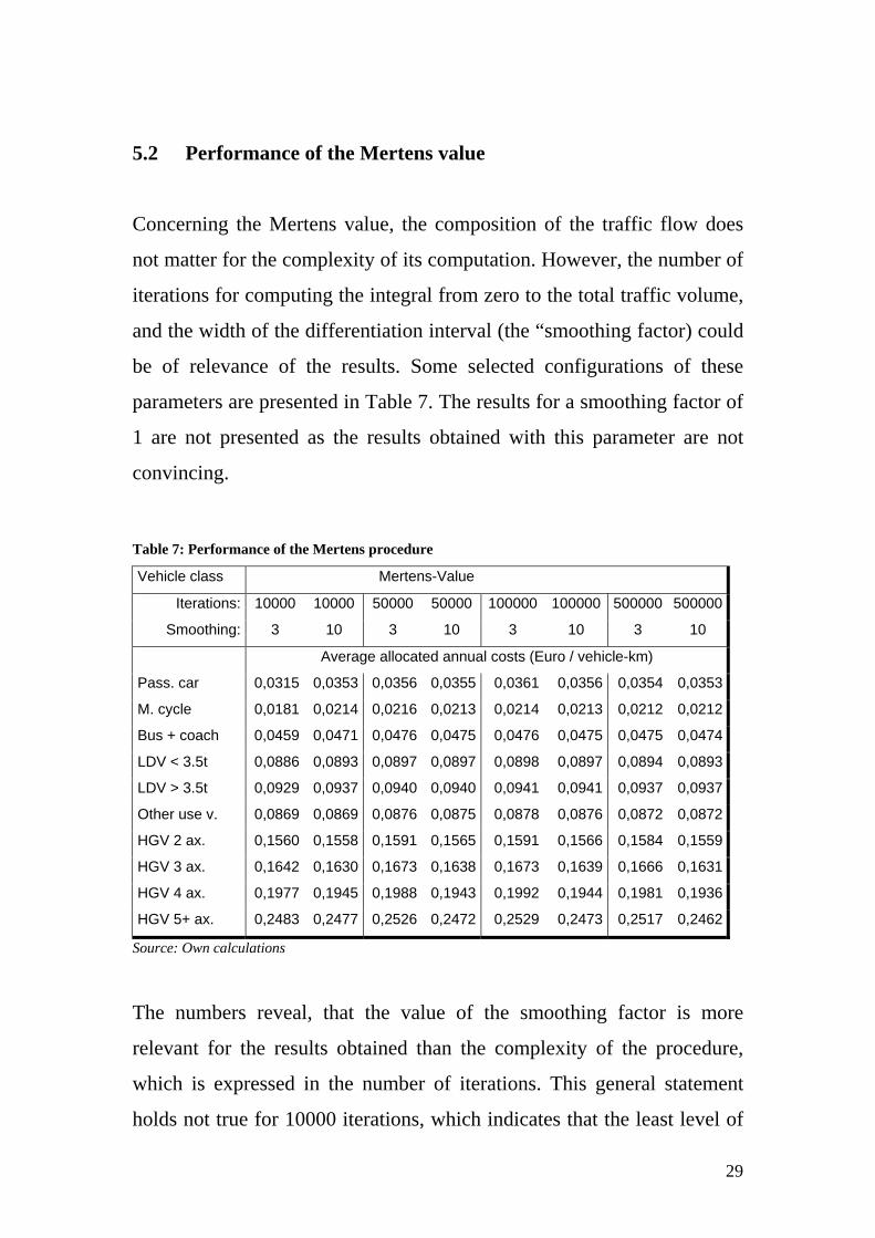
5.2 Performance of the Mertens value

Concerning the Mertens value, the composition of the traffic flow does

not matter for the complexity of its computation. However, the number of

iterations for computing the integral from zero to the total traffic volume,

and the width of the differentiation interval (the “smoothing factor) could

be of relevance of the results. Some selected configurations of these

parameters are presented in Table 7. The results for a smoothing factor of

1 are not presented as the results obtained with this parameter are not

convincing.

Table 7: Performance of the Mertens procedure

Vehicle class Mertens-Value

Iterations: 10000 10000 50000 50000 100000 100000 500000 500000

Smoothing: 3 10 3 10 3 10 3 10

Average allocated annual costs (Euro / vehicle-km)

Pass. car 0,0315 0,0353 0,0356 0,0355 0,0361 0,0356 0,0354 0,0353

M. cycle 0,0181 0,0214 0,0216 0,0213 0,0214 0,0213 0,0212 0,0212

Bus + coach 0,0459 0,0471 0,0476 0,0475 0,0476 0,0475 0,0475 0,0474

LDV < 3.5t 0,0886 0,0893 0,0897 0,0897 0,0898 0,0897 0,0894 0,0893

LDV > 3.5t 0,0929 0,0937 0,0940 0,0940 0,0941 0,0941 0,0937 0,0937

Other use v. 0,0869 0,0869 0,0876 0,0875 0,0878 0,0876 0,0872 0,0872

HGV 2 ax. 0,1560 0,1558 0,1591 0,1565 0,1591 0,1566 0,1584 0,1559

HGV 3 ax. 0,1642 0,1630 0,1673 0,1638 0,1673 0,1639 0,1666 0,1631

HGV 4 ax. 0,1977 0,1945 0,1988 0,1943 0,1992 0,1944 0,1981 0,1936

HGV 5+ ax. 0,2483 0,2477 0,2526 0,2472 0,2529 0,2473 0,2517 0,2462

Source: Own calculations

The numbers reveal, that the value of the smoothing factor is more

relevant for the results obtained than the complexity of the procedure,

which is expressed in the number of iterations. This general statement

holds not true for 10000 iterations, which indicates that the least level of

29

detail of the Mertens algorithm is somewhere between 10000 and 50000

items, However, Table 7 also reveals, that the algorithm is much more

stable than the extended Shapley procedure as the variations of average

costs ranges only within several percent.

5.3 The influence of network properties on the Mertens value

Table 8 presents some results obtained for nine different scenarios on the

network and transport volume input data. The following variables are

considered in the scenarios:

Age of assets: By default this parameter is set to 50% of the assets life

expectancy (LExp) as reported in Table 3. In addition, the network

scenarios consider a set of very new assets (age=0) and a set of written-

down assets (age=life expectancy). Due to the long life spans of many

road construction elements we observe difference in average costs of a

factor three to four across all vehicle classes.

HGV-Share: In the default case the share of HGVs is approximately 9%

of total traffic volume. Here, we consider higher values of 15%, 20% and

30%. It is interesting to observe, that the model outputs hardly react on

these changes. Thus, the tariffs calculated can be considered stable

against different traffic situations.

The reaction of the model for changing shares of fixed costs is tested

using the frost sensitivity class. This directly determines the thickness of

the frost preservation course. As the frost-save underground is determined

by the sum of the frost preservation course and the main course, this

construction element is not totally independent from traffic loads.

30

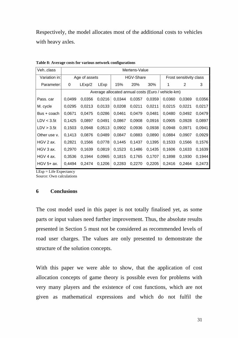
Respectively, the model allocates most of the additional costs to vehicles

with heavy axles.

Table 8: Average costs for various network configurations

Veh..class Mertens-Value

Variation in: Age of assets HGV-Share Frost sensitivity class

Parameter: 0 LExp/2 LExp 15% 20% 30% 1 2 3

Average allocated annual costs (Euro / vehicle-km)

Pass. car 0,0499 0,0356 0,0216 0,0344 0,0357 0,0359 0,0360 0,0369 0,0356

M. cycle 0,0295 0,0213 0,0133 0,0208 0,0211 0,0211 0,0215 0,0221 0,0217

Bus + coach 0,0671 0,0475 0,0286 0,0461 0,0479 0,0481 0,0480 0,0492 0,0479

LDV < 3.5t 0,1425 0,0897 0,0491 0,0867 0,0908 0,0916 0,0905 0,0928 0,0897

LDV > 3.5t 0,1503 0,0948 0,0513 0,0902 0,0936 0,0938 0,0948 0,0971 0,0941

Other use v. 0,1413 0,0876 0,0489 0,0847 0,0883 0,0890 0,0884 0,0907 0,0929

HGV 2 ax. 0,2821 0,1566 0,0778 0,1445 0,1437 0,1395 0,1533 0,1566 0,1576

HGV 3 ax. 0,2970 0,1639 0,0819 0,1523 0,1486 0,1435 0,1606 0,1633 0,1639

HGV 4 ax. 0,3536 0,1944 0,0965 0,1815 0,1765 0,1707 0,1898 0,1930 0,1944

HGV 5+ ax. 0,4494 0,2474 0,1206 0,2283 0,2270 0,2205 0,2416 0,2464 0,2473

LEsp = Life Expectancy Source: Own calculations

6 Conclusions

The cost model used in this paper is not totally finalised yet, as some

parts or input values need further improvement. Thus, the absolute results

presented in Section 5 must not be considered as recommended levels of

road user charges. The values are only presented to demonstrate the

structure of the solution concepts.

With this paper we were able to show, that the application of cost

allocation concepts of game theory is possible even for problems with

very many players and the existence of cost functions, which are not

given as mathematical expressions and which do not fulfil the

31

requirements of the space of functions pNA. By some refinements of the

original formulae of the Shapley value and the Aumann-Shapley-solution

for non-atomic games it was possible to reduce the usually excessive

computation times of these concepts to an acceptable level.

The advantage of game-theoretic solutions is, that we first agree on a

number of elementary fairness criteria, which should be fulfilled. Based

on these criteria we can select a mathematical solution concept. Further,

we have used standard engineering manuals to determine the

characteristic function of the game. This means, that the level of

arbitrariness, which is absolutely a point of criticism of the traditional

cost allocation procedures, which are usually applied on road track cost

accounting, can be substantially reduced.

REFERENCES

Aumann, R. J. and Shapley, L. S.: 1974. Values of Non-Atomic Games. 4

edn. Princeton University Press. Princeton, New Jersey. The Rand-

Cooperation.

Gritti, N. und Schweizer, M.: 2001. Schweizerische strassenrechnung

revision 2000. Technical report. Schweizerisches Bundesamt für

Statistik. Bern. Inofizielle Version.

Billera, L. J., Heath, D. C. and Raanan, J. 1978. Internal telephone billing

rates - a novel application of non-atomic game theory. Operation

Research 26(6), 956–965. Operations

32

Research Society of America.

Castano-Pardo, A. und Garcia-Diaz, A. 1995. Highway cost allocation

and the theory of nonatomic games. Transport Research, Part A 29A(3),

187–203. Elsewier Science Ltd, UK.

FGSV: 1976. Richtlinie für die Anlage von Landstraßen (RAL), Teil:

Knotenpunkte (RALK), Abschnitt 2: Planfreie Knotenpunkte (RAL-K-2).

Forschungsgesellschaft für Straßenund Verkehrswesen e.V.. Cologne.

FGSV290/5, Revised edition 1991.

FGSV: 1988a. Richtlinie für die Anlage von Straßen (RAS), Teil:

Knotenpunkte (RAS-K), Abschnitt 1: Plangleiche Knotenpunkte (RAS-K-

1). Forschungsgesellschaft für Straßen- und Verkehrswesen e.V..

Cologne. FGSV 297/1, Revised edition 1993.

FGSV: 1988b. Richtlinie für die Anlage von Straßen (RAS), Teil:

Leitfaden für die funktionale Gliederung des Straßennetzes (RAS-N).

Forschungsgesellschaft für Straßen- und Verkehrswesen e.V.. Köln.

FGSV 121.

FGSV: 1996. Richtlinie für die Anlage von Straßen (RAS), Teil:

Querschnitte (RAS-Q). Forschungsgesellschaft für Straßen- und

Verkehrswesen e.V.. Köln. FGSV 295.

FGSV: 2001b. Richtlinien für die Standardisierung des Oberbaus von

Verkehrsflächen (RstO-01). Forschungsgesellschaft für Straßen- und

Verkehrswesen e.V.. Köln.

33

FHWA: 1982. 1982 federal highway cost allocation study. Final report to

the Unites States Congress. Federal Highway Administration, U.S.

Department of Transportation. Washington D.C.

FHWA: 1997. Federal highway cost allocation study 2000. Final report

to the Unites States Congress HPP-10/9-98(3M)E. Federal Highway

Administration, U.S. Department of Transportation. Washington D.C.

Fragnelli, V., Garcia-Jurado, I., Norde, H., Patrone, F. und Tijs, S.: 1999.

How to share railway infrastructure costs. in I. Garcia-Jurado, F. Patrone

und S. Tijs (eds), Game Practice: Contribution from Applied Game

Theory. Kluwer. Dordrecht.

Herry, M., Rothengatter, W., Sedlacek, N., Doll, C., Visser, H., Quispel,

M., zek, S. S. and Klausegger, P.: 2002. Tarifrechnung

fahrleistungsabhängige Maut Österreich.. Report to the Austrian

Motorway and Express Road Financing Society (ASFINAG).

Ingenieurbüro Dr. Max Herry, IWW (Universität Karlsruhe), NEA,

Ingenieurbüro Snizek. Wien, Karlsruhe, Rijswijk.

Holler, M. J. and Illing, G.: 2000. Einführung in die Spieltheorie. 4 edn.

Springer Verlag. Berlin, Heidelberg.

Link, H., Rieke, H. und Schmied, M.: 2000.Wegekosten und

wegekostendeckung des straßen und schienenverkehrs in deutschland im

jahre 1997. Study commissioned by BGL e.V.. and ADAC e.V... Deutsches

Institut für Wirtschaftsforschung. Berlin.

34

Link, H., Steward, L. H. et al.: 2002. Pilot accunts - results for germany

and switzerland. unite (unification of accounts and marginal costs for

transpoert efficiency), deliverable 5. Accompanying measure financed by

the European Commission, DG-TREN, 5.framework programme,

Contract no.: 1999-AM.11157. DIW, Berlin. Leeds, Brüssel.

Koordinator: ITS, Univ. Leeds.

Littlechild, S. C. and Thompson, G. F. 1977. Aircraft landing fees: A

game theory approach.

The Bell Journal of Economics 8, 186–203.

Maerschalk G. 2001. Standardprognose des Erhaltungsbedarf der

Fernstraßeninfrastruktur bis 2015, interim report no. 5: Erhaltungsbedarf

der Brücken und sonstigen Ingenieurbauwerke; Ingenieurbüro SEP

Maerschalk. München.

Mertens, J. F.: 1988a. Nondifferentiable tu-markets: The value. in A. E.

Roth (ed.), The Shapley Value. Essays in Honor of Loyd S. Shalpey.

Cambridge University Press. Cambridge. pp. 235–264.

Mertens, J. F. 1988b. The shapley value in the non-differentiable case.

International Journal of Game Theory 17, 1–65.

Myerson, R. B.: 2001. Game Theory, Analysis of Conflict. 4. revised

edition, 2001 edn. Harvard University Press.

Shapley, L. S.: 1953. A value for n-person games. Contribution to the

Theory of Games. Vol. II, 28 of Anals of Mathematic Studies. H.W. Kuhn

and A.W. Tucker. Princeton. pp. 307– 317.

35

Rommerskirchen, S., Rothengatter, W., Helms, M., Doll, C., Liedtke, G.

and Vödisch, M.: 2002. Wegekostenrechnung für das

bundesfernstraßennetz unter berücksichtigung der vorbereitung einer

streckenbezogenen autobahnbenutzungsgebühr. F+E-Bericht 96

693/2001. Bundesminister für Verkehr, Bau und Wohnungswesen.

Berlin.

36