Faculteit Wiskunde en Informatica

bdeweger

Stamp

Acknowledgements.

The research on which this book reports has been done while I worked for the

Netherlands Foundation for Mathematics SMC, with financial support from the

Netherlands Organization for the Advancement of Pure Research ZWO. This

research took place from 1983 to 1987 at the University of Leiden, under

supervision of Professor R. Tijdeman and Dr. F. Beukers.

I am very grateful to my (number theory) teacher, Professor R. Tijdeman

(Leiden), for suggesting the research topic, for all his help, comments and

criticism, on mathematics and everything else. I am also indebted to:

-----L Dr. F. Beukers (Utrecht), for comments and discussions,

-----L Dr. A. Petho (Debrecen), my first coauthor, for the cooperation, the

hospitality in Cologne in february 1985, and for allowing me to publish our

joint work in Chapter 4 of this book,

-----L Prof. N. Tzanakis (Iraklion), my other coauthor, for the cooperation, the

many discussions, the hospitality in Iraklion in october-november 1986, for

allowing me to publish our joint work in Chapter 8 of this book, and for

pointing out some errors in the manuscript,

-----L Prof. L. Wang (Beijing), for carefully checking most of the computations

of Chapter 6, and thus finding some errors,

-----L Dr. B.H. Gilding (Enschede), for polishing some of the english,

-----L the Faculty of Applied Mathematics of the University of Twente (Enschede),

for providing a good working environment and computing and text-editing

facilities,

-----L the Dutch Open University (Heerlen), for (unintentionally) providing text-

editing facilities,

and finally to Alda, for being there and loving me.

SOLI DEO GLORIA.

Benne de Weger,

University of Twente,

Enschede, The Netherlands. February 1989.

(v)

Contents.

Chapter 1. Introduction. 1

S 1.1. Algorithms for diophantine equations. 1

S 1.2. The Gelfond-Baker method. 9

S 1.3. Theoretical diophantine approximation. 12

S 1.4. Computational diophantine approximation. 14

S 1.5. The procedure for reducing upper bounds. 22

Chapter 2. Preliminaries. 24

S 2.1. Algebraic number theory. 24

S 2.2. Some auxiliary lemmas. 26

S 2.3. p-adic numbers and functions. 27

S 2.4. Lower bounds for linear forms in logarithms. 29

S 2.5. Numerical methods. 32

Chapter 3. Algorithms for diophantine approximation. 36

S 3.1. Introduction. 36

S 3.2. Homogeneous one-dimensional approximation in the real

case: continued fractions. 37

S 3.3. Inhomogeneous one-dimensional approximation in the

real case: the Davenport lemma. 39

3S 3.4. The L -lattice basis reduction algorithm, theory. 41

3S 3.5. The L -lattice basis reduction algorithm, practice. 45

S 3.6. Finding all short lattice points: the Fincke and Pohst

algorithm. 51

S 3.7. Homogeneous multi-dimensional approximation in the

real case: real approximation lattices. 53

S 3.8. Inhomogeneous multi-dimensional approximation in the

real case: an alternative for the generalized

Davenport lemma. 56

S 3.9. Inhomogeneous zero-dimensional approximation in the

p-adic case. 60

(vi)

S3.10. Homogeneous one-dimensional approximation in the

p-adic case: p-adic continued fractions and

approximation lattices of p-adic numbers. 61

S3.11. Homogeneous multi-dimensional approximation in the

p-adic case: p-adic approximation lattices. 63

S3.12. Inhomogeneous one- and multi-dimensional approximation

in the p-adic case. 64

S3.13. Useful sublattices of p-adic approximation lattices. 66

Chapter 4. S-integral elements of binary recurrence sequences. 70


S 4.2. Binary recurrence sequences. 72

S 4.3. The growth of the recurrence sequence. 74

S 4.4. Upper bounds. 80

S 4.5. A basic lemma. 82

S 4.6. Trivial cases. 83

S 4.7. The reduction algorithm in the hyperbolic case. 88

S 4.8. The reduction algorithm in the elliptic case. 92

S 4.9. The generalized Ramanujan-Nagell equation. 95

S4.10. A mixed quadratic-exponential equation. 99

dChapter 5. The inequality 0 < x - y < y in S-integers. 102


S 5.2. Upper bounds for the solutions. 103

S 5.3. Reducing the upper bounds in the one-dimensional case. 104

S 5.4. Reducing the upper bounds in the multi-dimensional case. 106

S 5.5. Tables. 110

Chapter 6. The equation x + y = z in S-integers . 115



S 6.3. The p-adic approximation lattices. 118

S 6.4. Reducing the upper bounds in the one-dimensional case. 120

S 6.5. Reducing the upper bounds in the multi-dimensional case. 123

S 6.6. Examples related to the abc-conjecture. 125

S 6.7. Tables. 127

(vii)

Chapter 7. The sum of two S-units being a square. 136


S 7.2. The case D = 1 . 137

S 7.3. Towards generalized recurrences. 138

S 7.4. Towards linear forms in logarithms. 142

S 7.5. Upper bounds for the solutions: outline. 147

S 7.6. Upper bounds for the solutions: details. 150

S 7.7. The reduction technique. 158

S 7.8. The standard example. 158

S 7.9. Tables. 168

Chapter 8. The Thue equation. 178


S 8.2. From the Thue equation to a linear form in logarithms. 179


S 8.4. Reducing the upper bound. 188

S 8.5. An application: triangular numbers that are a product

of three consecutive numbers. 191

S 8.6. The Thue-Mahler equation, an outline. 202

References. 205

(viii)

Chapter 1. Introduction.

1.1. Algorithms for diophantine equations.

This monograph deals with certain types of diophantine equations. An equation

is a mathematical formula, expressing equality of two expressions that

involve one or more unknowns (variables). Solving an equation means finding

all solutions, i.e. the values that can be substituted for the unknowns such

that the equation becomes a true statement. An equation is called a

diophantine equation if the solutions are restricted to be integers in some

sense, usually the ordinary rational integers (elements of Z ) or some

subset of that.

Examples of diophantine equations that will be studied in this book are

2 nx + 7 = 2

(the Ramanujan-Nagell equation, having only the solutions given by

(+x,n) = (1,3), (3,4), (5,5), (11,7), (181,15) , see Chapter 4);

x y z2 = 3 + 5

(a purely exponential equation, having only the solutions (x,y,z) = (1,0,0),

(2,1,0), (3,1,1), (5,3,1), (7,1,3) , see Chapter 6);

2 3y = x - 4Wx + 1

(an elliptic curve equation, having only 22 solutions, of which the largest

are (x,y) = (1274,+45473) , see Chapter 8). The three examples mentioned

here are only some examples; we will study much wider classes of equations.

We also study (in Chapter 5) a diophantine inequality (a formula expressing

that one expression is larger than another, where solutions are again

restricted to integers). In the following discussion the statements about

diophantine equations also hold for this inequality.

What the equations treated in this book have in common is that they can all

be solved by the same method. This method consists essentially of three

1

parts: a transformation step, an application of the Gelfond-Baker theory, and

a diophantine approximation step. We explain these steps briefly.

To start with, one transforms the equation into a purely exponential equation

or inequality, i.e. a diophantine equation or inequality where the unknowns

are all in the exponents, such as in the second example given above. Each

type of diophantine equation needs a particular kind of transformation, so

that it is difficult to be more specific at this point. In some instances,

such as in the second example above, this transformation is easy, if not

trivial. In other instances, as in the first example above, it uses some

arguments from algebraic number theory, or, as in the third example above, a

lot of them.

In general, such a purely exponential equation has the form

s st i n 0 n

ij 0jS c W p a = c W p a , (1.1)

i ij 0 0ji=1 j=1 j=1

and a corresponding purely exponential inequality looks like

s st i n i n d

| ij| | ij|| S c W p a | < min|c W p a | (1.2)| i ij | | i ij |i=1 j=1 i j=1

where t, s , c , a , d are constants with t, s e N , 0 < d < 1 , andi i ij i

c , a belong to some algebraic extension of Q , and where the n arei ij ijthe unknowns in Z . We now suppose that the number of terms t on the left

hand side of (1.1) or (1.2) is equal to 2 . This restriction is essential

for the second step, in which we use results from the so-called theory of

linear forms in logarithms, also known as the Gelfond-Baker theory. (Some

special exponential equations of type (1.1) with t > 2 can also be treated

by the Gelfond-Baker method, since they can be reduced to exponential

inequalities of type (1.2) with t = 2 , cf. Stroeker and Tijdeman [1982],a b

Alex [1985 ], [1985 ], Tijdeman and Wang [1988].)

An exponential equation or inequality such as (1.1) or (1.2) with t = 2

gives rise to a linear form in logarithms

mL = log b + S n Wlog b ,

0 i ii=1

where the b are algebraic constants, and the n are integral unknowns.i i

Here, the logarithms are real or complex in some instances, or p-adic in

2

other cases. This relation between equation and linear form in logarithms is

such that for a large solution of the equation the linear form is extremely

close to zero (in the real or complex sense, or in the p-adic sense). The

Gelfond-Baker theory provides effectively computable lower bounds for the

absolute values (respectively p-adic values) of such linear forms in

logarithms of algebraic numbers. In many cases these bounds have been

explicitly computed. Comparing the so-found upper and lower bounds it is

possible to obtain explicit upper bounds for the solutions of the exponential

diophantine equation or inequality, leading to upper bounds for the solutions

of the original equation. This second step, unlike the first (transformation)

step, is of a rather general nature.

We remark that many authors have given effectively computable upper bounds

for the solutions of a wide variety of diophantine equations, by applying the

method sketched above. For a survey, see Shorey and Tijdeman [1986]. Often

these authors were satisfied with the knowledge of the existence of such

bounds, and they did not actually compute them. If they computed bounds, they

did not always determine all the solutions. In this book, solving an equation

will always mean: explicitly finding all the solutions.

After the second step, the problem of solving the diophantine equation is

reduced to a finite problem, which is treated in the third part of the

method. Namely, since we have found explicit upper bounds for the absolute

values of the (integral) unknowns, we have to check only finitely many

possibilities for the unknowns. However, the word finite does not mean the

same as small or trivial. In fact, the constants appearing in the lower

bounds that the Gelfond-Baker theory provides for linear forms in logarithms

are rather large. Therefore, in practice the upper bounds that can be

obtained in this way for the solutions of purely exponential equations can be40

for instance as large as 10 . This is far too large to admit simple

enumeration of all the possibilities, even with the fastest of computers

today.

Proving the existence of an absolute upper bound for the solutions reduces

the determination of all the solutions from an infinite task to a finite one.

Thus, the application of the Gelfond-Baker theory (the second step) is in a

sense infinitely many times as difficult a task than the only finite amount

of checking that remains to be done (in the third step). Furthermore, this

checking seems to be a technical problem only, not a mathematical one.

3

Nevertheless, it is the author’s opinion that solving this comparatively

small technical problem is not only nontrivial, but involves some serious and

interesting mathematics. This book hopefully illustrates this opinion.

Notwithstanding the fact that the application of the Gelfond-Baker theory in

the second step yields very large upper bounds, it is generally assumed that

these upper bounds are far from the actual largest solution. Therefore, it is

worthwile to search for methods to reduce these upper bounds to a size that

can be more easily handled. Often it is possible to devise such a method

using directly certain properties of the original diophantine equation, for

example that large solutions must satisfy certain congruences modulo many or

large numbers (Grinstead [1978], Brown [1985], Pinch [1988]), or some

reciprocity condition (Petho [1983]). The disadvantage of such methods is

that they work only for that particular type of diophantine equation, so that

in general for each type of equation a new reduction method must be devised.

It would therefore be interesting to have methods for reducing upper bounds

for the solutions of inequalities for linear forms in logarithms. They would

be useful for solving any type of diophantine problem that leads to such

inequalities.

Such methods are searched for in the third step of our method of solving

diophantine equations. It is mainly in this third part that new developments

can be reported. The arguments we use in the first and second parts are

mainly classical, and we apply them to types of equations that have been

studied before, and also to new types of equations.

The methods that are needed in the third step are provided by that part of

the theory of diophantine approximation that is concerned with studying how

close to zero a linear form can be for given values of the variables.

Recently important progress has been made in this field, the breakthrough3

being the invention in 1981 by L. Lovssz of the so-called L -laticce basis3

reduction algorithm. We will show how this L -algorithm leads to practically

efficient diophantine approximation algorithms, which can be employed for

many diophantine equations to show that in a certain interval [X ,X ] no1 0

solutions exist. Usually X is of the order of magnitude of log X . When1 0

for X the theoretical upper bound for the solutions is substituted, a new,0

and usually much better upper bound X is found. For many equations the1

initial upper bound X is well within reach of practical application of0

these algorithms, within only a few minutes of computer time. This thus leads

4

in practice to methods for finding all the solutions of many types of

diophantine equations, for which alternative methods have not yet been found

or employed with success.

The method outlined above, and used in this book to solve many examples of

various diophantine equations, is of an "algorithmic" nature. In a sense it

lies between "ad hoc" methods and "theoretical" methods. This we shall

explain below. Let a set of diophantine equations with an unspecified

parameter in it be given. As an example of such a set, consider the2 n

generalized Ramanujan-Nagell equation x + D = 2 , where D is a

parameter, and x, n are the unknowns.

An ad hoc method is a method for solving the equation for specific values of

the parameters only. It may not work at all for other than these particular2 n

values. The first example of solving an equation of the type x + D = 2

occurring in the literature is that by Nagell [1948] of D = 7 . The method

he used is of an ad hoc nature, since it depends heavily on the special

choice of 7 for the parameter D .

A theoretical method is capable of proving results that hold for some large

set of values of the parameters. The Gelfond-Baker theory is of a theoretical

nature, since it yields upper bounds for the solutions of many equations in

terms of their parameters. Other examples are application of the theory of2 n

quadratic reciprocity, that shows that x + D = 2 has no solutions at all

if D is odd, at least 5 , and not congruent to 7 (mod 8) , and

application of the theory of hypergeometric functions, which Beukers [1981]2 n

used to show that the solutions (x,n) of x + D = 2 satisfy2 96 2

n < 435 + 10W log|D| , and if |D| < 2 then moreover n < 18 + 2W log|D| .

Theoretical methods are often too general to be able to produce all the

solutions of a given equation.

An algorithmic method is a method that is guaranteed to work for any set of

values of the parameters, but has to be applied separately to each particular

set of parameter values, in order to produce all the solutions. The methods

used in this book are mainly of such an algorithmic nature. For the equation2 nx + D = 2 (and actually for a more general equation) we will give an

algorithmic method in Chapter 4. In fact, since Beukers’ above-mentioned

result provides a small upper bound for the solutions, it can be made

algorithmic by providing a simple method of enumerating all the solutions

5

below the upper bound. However, the algorithmic part of this method is

trivial, and therefore we still prefer to classify Beukers’ method as

theoretical. In order to make the Gelfond-Baker theory algorithmic,

enumeration of all possibilities is impractical. Therefore more ingenious

ways of determining all the solutions below a large upper bound have to be

found. We remark that Beukers’ method for the more general equation2 nx + D = p also has an ad hoc aspect, since it works for some special

values of p only. Our method of Chapter 4 does not have this disadvantage.

An ideal towards which one might strive in solving diophantine equations is

to devise a computer algorithm, a kind of ’diophantine machine’, which only

has to be fed with the parameters of the equation, and after a short time

gives as output a list of all the solutions. One should have a guarantee (in

the strictest mathematical sense of proof) that no solutions are missing.

At first sight the method outlined above, and described in this monograph,

seems to be a good candidate to be developed into such a general applicable

algorithm. Namely, the second step is of a quite general nature, providing

upper bounds for exponential diophantine equations that are explicit in the

parameters of the equation. Also the third step, the algorithmic diophantine

approximation part, works in principle for any set of values substituted for

the parameters. However, the computations have to be performed separately for

each particular set of values.

The main difficulties in devising such a ’diophantine machine’ are in the

first part of the method outlined above, especially if some algebraic number

theory is used. Developments taking place in the theory of algorithmic

algebraic number theory on computing fundamental units and on finding

factorizations of prime numbers in algebraic extensions, are of importance

here. We believe that when suitable algorithms of this kind are available, it

will be possible in principle to make such a ’diophantine machine’ (but

technical difficulties in the third step should not be underestimated). The

generality of such an algorithm is restricted by the generality of the first

step, the transformation to the linear form in logarithms. In this book we

use computer algorithms only if the magnitude of the computational tasks

makes this necessary, and keep to "manual" work otherwise. In this way we

also try to keep the presentation of the methods lucid.

The reader should be aware of the fact that the computer programs and their

6

results are part of the proofs of many of our theorems on specific

diophantine equations. It is however impossible to publish all details of

these programs and computations. The interested reader may obtain the details

from the author by request, and is invited to check the computations himself.

The book by Shorey and Tijdeman [1986] gives a good survey of the diophantine

equations for which computable upper bounds for the solutions can be found

using the Gelfond-Baker method (see also Shorey, van der Poorten, Tijdeman

and Schinzel [1977], and Stroeker and Tijdeman [1982]). Some of these

equations can be completely solved by the methods described in this book,

among which there are purely exponential equations, equations involving

binary recurrence sequences, and Thue equations and Thue-Mahler equations.

Especially the latter two are of importance in various other parts of number

theory. For example, they are the key to solving Mordell equations and

various equations arising in algebraic number theory and arithmetic algebraic

geometry. The Gelfond-Baker method was used to actually solve a diophantine

equation for the first time in the work of Baker and Davenport [1969] in

solving the system of diophantine equations

2 2 2 23Wx - 2 = y , 8Wx - 7 = z .

Other equations occuring in the literature for which upper bounds for the

solutions can be computed, cannot be treated as easily by our algorithmic

methods, because the application of the theory of linear forms in logarithms

is more complicated for these equations, and moreover the upper bounds are

essentially too large. An example of this kind is the Catalan equationx ya - b = 1 in integers a, b, x, y , all > 2 . Catalan conjectured in 1844

that this equation has only the solution (a,b,x,y) = (3,2,2,3) . Tijdeman

[1976] proved that the solutions of the Catalan equation are bounded by a

computable number. This number can be taken to be exp(exp(exp(exp(730)))) ,

according to Langevin [1976]. However, we fail to see how the methods that we

describe in the forthcoming chapters can be applied for completely solving

the Catalan equation, and we believe that Grosswald’s remarks on this topic

are too optimistic (Grosswald [1984], p. 259, in particular the footnote).

Another diophantine equation, that for centuries has attracted the attentionn n n

of many mathematicians, is the Fermat equation x + y = z in integers x,

y, z, n , with n > 3 and xWyWz $ 0 . It is conjectured to have no

solutions. Faltings [1983] proved that for fixed n the number of solutions

7

is finite. His proof is ineffective. The Gelfond-Baker theory seems not to be

strong enough to deal with the Fermat equation in its full generality, not

even if n is fixed. For a survey of partial results on the Fermat equation

that have been obtained using this theory, see Tijdeman [1985] and Chapter 11

of Shorey and Tijdeman [1986].

We remark that for many diophantine equations recently important progress has

been made in determining upper bounds for the number of solutions. See e.g.

Evertse [1983], Evertse, Gyory, Stewart and Tijdeman [1988] and Schmidt

[1988] for a survey. These results are often remarkably sharp, but

ineffective, so that they cannot be used for actually finding the solutions.

To conclude this section we give an overview of the contents of this

monograph. It is divided into three parts: Chapter 1 is introductory,

Chapters 2 and 3 give the necessary preliminaries, and Chapters 4 to 8 deal

with various types of diophantine equations.

Sections 1.2 to 1.5 give a short introduction for the non-specialist to

respectively the Gelfond-Baker theory, diophantine approximation theory, the

algorithmic aspects of diophantine approximation, and the procedure for

reducing upper bounds. Chapter 2 contains the preliminary results that we

need from algebraic number theory and from the theory of p-adic numbers and

functions, and quotes in full detail the theorems from the Gelfond-Baker

theory which we use. It concludes with some remarks on numerical methods.

Chapter 3 gives in detail the algorithms in the field of diophantine

approximation theory that we apply in the subsequent chapters. In a sense

this chapter is the heart of the book.

Chapters 4 to 8 are each devoted to a certain type of diophantine equation.

Let p , ..., p be a fixed set of distinct primes. Let S be the set of1 s

positive integers composed of primes p , ..., p only.1 s

Chapter 4 deals with elements of binary recurrence sequences ("generalized

Fibonacci sequences") that are in S , and gives applications to mixed

quadratic-exponential equations, such as the generalized Ramanujan-Nagell2

equation x + k e S ( k fixed). The diophantine approximation part of this

chapter is interesting for two reasons: the p-adic approximation is very

simple, and in the case of the recurrence having negative discriminant, a

nice interplay of p-adic and real/complex approximation arguments occurs. The

8

research for Chapter 4 was done partly in cooperation with A. Petho from

Debrecen. The results have been published in Petho and de Weger [1986] and deb

Weger [1986 ].

dChapter 5 deals with the diophantine inequality 0 < x - y < y , where

x, y e S , and d e (0,1) is fixed. Chapter 6 deals with x + y = z , where

x, y, z e S , which can be considered as the p-adic analogue of the

inequality of Chapter 5. These two equations are the simplest examples of

diophantine equations that can be treated by our method. Since they are

already purely exponential equations of the form (1.1) or (1.2) with t = 2 ,

the first step is trivial: the linear forms in logarithms are directly

related to the equations. Therefore they serve as good examples to get a

clear understanding of the diophantine approximation part of our method. The

results of these chapters have been published in de Weger [1987].

2Chapter 7 studies the equation x + y = z , where x, y e S , and z e Z .

This equation is a further generalization of the generalized Ramanujan-Nagell

equation, studied in Chapter 4.

In Chapter 8 a procedure is given to solve Thue equations, that works in

principle for Thue equations of any degree. It is applied to find all2 3

integral points on the elliptic curve y = x - 4Wx + 1 . We also mention

briefly how Thue-Mahler equations can be dealt with. This chapter has been

written jointly with N. Tzanakis from Iraklion. The results have beena a

published in Tzanakis and de Weger [1989 ], and in de Weger [1989 ].

1.2. The Gelfond-Baker method.

In Section 1.1 we have explained that before applying the Gelfond-Baker

method to some diophantine equation, the equation should be transformed into

a purely exponential diophantine equation or inequality with not too many

terms (cf. (1.1), (1.2)). In this section we sketch the arguments from the

Gelfond-Baker theory that lead to upper bounds for the variables of this

exponential equation/inequality.

Let us first treat the case of the inequality (1.2). Since t = 2 we may

assume that it has the form

9

s n| i || a W p a - 1 | < C Wexp(-dWN) ,| 0 i | 0

i=1

where the a are fixed algebraic numbers, N = max|n | , and C , d arei i 0

positive constants. In the examples we study, we encounter one of the

following two cases: either all a are real, or |a | = 1 for all i . Ini i

the real case, if N is large enough, the linear form in logarithms

sL = log|a | + S n Wlog|a |

0 i ii=1

must satisfy

|L| < C’Wexp(-dWN) (1.3)0

for some C’ . In the complex case, the same inequality (1.3) follows for the0

linear form

sL = Log a + S n WLog a + kWLog(-1)

0 i ii=1

s( )

= iW Arg a + S n WArg a + kWp ,9 0 i i 0

i=1

where the Log and Arg functions take their principal values. Now we can

apply one of the many results from the Gelfond-Baker theory, giving an

explicit lower bound for |L| in terms of N , e.g. the following theorem.

THEOREM_1.1._(Baker_[1972]). Let L be as above. There exist computable

constants C , C , depending on the a only, such that if L $ 0 then1 2 i

( )|L| > exp -(C +C Wlog N) .

9 1 2 0

We usually know that L $ 0 . Combining (1.3) and Theorem 1.1 we then obtain

C + log C’ C1 0 2

N < ------------------------------------------------------- + ----------Wlog N .d d

It follows that N is bounded from above.

Next, consider the exponential equation (1.1). By t = 2 we can write it as

s n r mi j

a W p a - 1 = b W p b ,0 i 0 ji=1 j=1

10

where the a , b are fixed algebraic numbers. Let H be the maximum ofi j p

the |n |, |m | where i, j run through the set of indices for which ai j i

resp. b are non-units. Let H be the maximum of the |n |, |m | wherej i j

i, j run through the set of all indices. Suppose that p is a rational

prime lying above b for some j . There are constants c , c such thatj 1 2

s n( i )

ord a W p a -1 > c + c Wm .p9 0 i 0 1 2 j

i=1

Assuming that ord (a ) = 0 for all i , we may write down a p-adic linearp i

form in logarithms

sL = log a + S n Wlog a ,

p 0 i p ii=1

for which, if m is large enough, it follows thatj

ord (L) > c + c Wm . (1.4)p 1 2 j

We are now in a position to apply the following result from the p-adic

Gelfond-Baker theory. Here, N = max|n | .i

THEOREM_1.2._(van_der_Poorten_[1977],_Yu_[1987]). Let L , p be as above.

There exist computable constants C , C , depending only on the a and on3 4 i

p , such that if L $ 0 then

ord (L) < C + C Wlog N .p 3 4

Applying (1.4) and Theorem 1.2 for all possible p we obtain constants C’,3

C’ with4

H < C’ + C’Wlog H .p 3 4

If H < C WH for some constant C , then this immediately yields an upper5 p 5

bound for H . If H > C WH , then it can be shown that there exists a5 p

conjugate of the a , b , denoted with a prime sign, for whichi j

r m| j||b’W p b’ | < exp(-C WH)| 0 j | 6

j=1

for a constant C (cf. the proof of Theorem 1.4, pp. 45-49, of Shorey and6

Tijdeman [1986]). Now we can apply Theorem 1.1. This yields

11

s n| i | ( )|a’W p a’ -1| > exp -(C +C Wlog H) .| 0 i | 9 7 8 0

i=1

It follows that H is bounded from above.

If it happens that none of the a , b are units, then of course thei j

application of Theorem 1.2 suffices.

We remark that, in order to be able to completely solve a diophantine

equation, it is crucial that all constants can be computed explicitly.

Therefore we can only use the bounds from the Gelfond-Baker theory that are

completely explicit. We give details of such theorems in Section 2.4.

1.3. Theoretical diophantine approximation.

In this section we briefly mention some results from diophantine

approximation theory, thus giving a background to the next section. We refer

to Koksma [1937], Cassels [1957] (Chapters I and III) and to Hardy and Wright

[1979] (Chapters XI and XXIII), for further details.

The simplest form of diophantine approximation in the real case is that of

approximation of a real number y by rational numbers p/q . It is well

known that if y is irrational, then there exist infinitely many solutions

(p,q) e Z*N with (p,q) = 1 of the diophantine inequality

p -2| y - ----- | < q .

q

All convergents from the continued fraction expansion of y are such

solutions. The convergents are simple to compute for any particular y e R .

One way of generalizing this is to study simultaneous approximations to a set

of real numbers y , ..., y , i.e. rational approximations to y all1 n i

having the same denominator. It is well known that the system of inequalities

pi -(1+1/n)

| y - ---------- | < q for i = 1, ..., ni q

has infinitely many solutions (p ,...,p ,q) if at least one of the y is1 n i

irrational. But it is much harder to find solutions of such inequalities than

in the case n = 1 . Some multi-dimensional continued fraction algorithms

12

have been devised (cf. Brentjes [1981] for a survey), but they seem not to

have the desired simplicity and generality. We shall see later how we can3

apply the so-called L -algorithm to this problem.

Another way of generalizing the simplest case of diophantine approximation is

to study linear forms, such as

mL = S q Wy ,

j jj=1

where y , ..., y are given real numbers, and q , ..., q are the1 m 1 m

unknowns in Z . Put Q = max|q | . A classical theorem guarantees thei

existence of a solution (p,q ,...,q ) of the inequality1 m

-m| L - p | < Q .

Note that the case m = 1 becomes our first inequality on dividing by3

q = q . Also in this case the L -algorithm is very useful, as we shall see1

below.

We can incorporate the two generalizations above in a further generalization,

that of simultaneous approximation of linear forms. Let real numbers y beij

given for i = 1, ..., n , j = 1, ..., m . Put

mL = S q Wy for i = 1, ..., n .i j ij

j=1

A celebrated theorem of Minkowski states that there exists a solution

(p ,...,p ,q ,...,q ) of the system of inequalities1 n 1 m

-m/n| L - p | < Q for i = 1, ..., n .

i i

3As we shall show in Section 1.4, the L -algorithm may be applied to this

general form. We actually compute solutions of systems of inequalities that

are slightly weaker in the sense that the right hand side is multiplied by a

small constant larger than 1.

We now consider inhomogeneous approximation. This means that for all i

there is an inhomogeneous term b in the linear form L , viz.i i

mL = b + S q Wy for i = 1, ..., n .i i j ij

j=1

Again, there exists a constant c such that the system

13

-m/n| L - p | < cWQ for i = 1, ..., n ,

i i

under some independence condition on the b and y , has a solution. Thisi ij

is Kronecker’s theorem. The simplest case m = n = 1 comes down to

-1| qWy - p + b | < cWq .

The upper bounds given above, that tell us that the order of magnitude of-m/n

| L - p | can be at least as small as Q , are not only theoreticali i

upper bounds, but they predict the heuristically expected order of magnitude

as well. By this we mean that in a generic situation (i.e. when there are no

almost-linear relations between the y (and the b ), it is indeed theij i

case that for a given Q the minimal max|L -p | , taken over all Q < Q ,0 i i 0

i-m/n

has the order of magnitude of the upper bound Q .

To conclude this section, we remark that there is a p-adic analogue of this

theory of diophantine approximation, founded by Mahler and Lutz. If we

replace in the above considerations R by Q , the absolute value |W| byp

the p-adic value |W| , and the measure Q for an approximationp

n+m(p ,...,p ,q ,...,q ) by any convex norm F(p ,...,p ,q ,...,q ) on R ,1 n 1 m 1 n 1 m

then the p-adic analogues of the theorems of Minkowski and Kronecker are

essentially analogous to the above mentioned results in the real case. See

Koksma [1937] for references to Mahler’s work, and Lutz [1951], and for aa

detailed analysis of the case n = 1 , m = 2 see de Weger [1986 ].

1.4. Computational diophantine approximation.

In this section we give some idea of practically solving the diophantine

approximation problems that we encounter in solving diophantine equations. In

this section we give no rigorous treatment. We neglect worst cases, and

concentrate on how things are expected to work (according to the heuristics

of Section 1.3), and appear to work in practice. In the subsequent chapters

many examples are given, showing that our methods are indeed useful in

practice. Applying the method in practice may be the best way of acquiring"

the necessary Fingerspitzengefuhl for the method.

We shall deal with the following computational diophantine approximation

14

problem. Let y , b e R be given, and let p , ..., p , q , ..., q beij i 1 n 1 m

integral unknowns with Q = max|q | . Let L be as above. Let a positivej i

50constant Q , assumed to be a rather large number, 10 say, be given.

0Find a lower bound for the value of

max | L - p | ,i i

i

where (p ,...,p ,q ,...,q ) runs through the set of values with Q < Q .1 n 1 m 0

From the heuristics outlined in Section 1.3 it follows that one will be-m/n

satisfied if this lower bound is of the size Q . For the p-adic case an0

analogous problem may be formulated.

Related problems in diophantine approximation theory are those of actually

finding a good or the best solution of max|L -p | < e for a fixed e > 0 .i i

i3

As we shall see, the L -algorithm is a very useful tool for finding good

solutions. The problem of finding the best solution however seems to be

essentially more difficult. We note that in most of our applications of

solving diophantine equations it suffices to have a suitable lower bound for

max|L -p | for a given Q , while it is unnecessary to know explicitly howi i 0

isharp this bound is.

The computational tool that we use to solve the afore-mentioned problems is3

the so-called L -lattice basis reduction algorithm, described in Lenstra,

Lenstra and Lovssz [1982]. We shall give details of this algorithm in

Sections 3.4 and 3.5. Below we briefly indicate how it can be used to solve

diophantine approximation problems.

n 3Let G be a lattice in R . The L -algorithm accepts as input an arbitrary

basis b , ..., b of G . As output it gives another basis c , ..., c of1 n 1 n

the same lattice G , that is a so-called reduced basis. The concept reduced

means something like nearly orthogonal. From a reduced basis it is possible

to compute lower bounds for the following two quantities:

-----L the length of the non-zero lattice point that is nearest to the origin:

l(G) = min |x| ,0$xeG

(see Lenstra, Lenstra and Lovssz [1982], Prop. (1.11), and our Lemma 3.4),

15

n-----L for any given point y e R , the distance from y to the nearest lattice

point:

l(G,y) = min |x-y| ,xeG

(see Babai [1986], and our Lemmas 3.5 and 3.6).

3The L -algorithm enjoys the property that these lower bounds are usually near

to the actual minimal solutions. In a generic situation, where the lattice is

not too distorted, the vectors c of the reduced basis all have about thei

same length, which is of the order of magnitude of

1/ndet(G) .

The value of l(G) as well as the lower bounds computed for it, are about as

large as that. If y is not too close to a lattice point, the same holds for

l(G,y) . Moreover, the running time of the algorithm is good, both in the

theoretical sense (it is polynomial-time in the length of the input-

parameters), and in practice (cf. Lenstra [1984], p. 7).

To solve the problem of finding a lower bounds for max|L -p | as formulatedi i

iabove, we take the lattice G as follows. Let C be an integer, at least as

1+m/nlarge as Q . The lattice G , of dimension n + m , is defined by

0specifying a basis, namely the column vectors b , ..., b of the matrix

1 n+m

& 1 *.

| . o |.

| o |1

| |B = | [CWy ] ... [CWy ] -C | .

11 1m| . . . |

. . .| . . . |

o| |[CWy ] ... [CWy ] -C

7 n1 nm 8

(The symbol o means that all not explicitly given entries in that area are3

zero). Applying the L -algorithm to this lattice we find a reduced basis, ofn/(m+n)

which the basis vectors will have lengths of about C , which is

roughly the size of Q . Generally speaking, the larger C is, the larger0

the lengths of the basis vectors of a reduced basis will be (and the larger

the lower bounds for l(G) and l(G,y) will be).

Let us first treat the homogeneous case, i.e. b = 0 for all i . Consideri

16

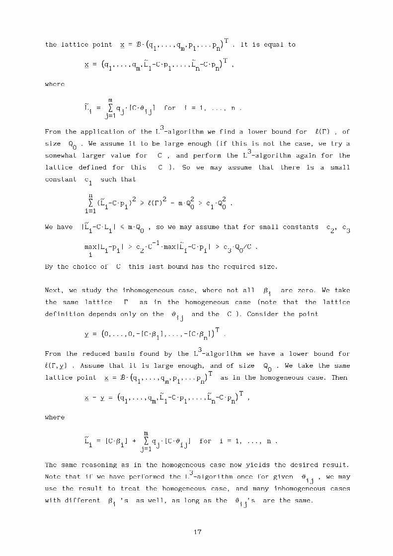
( )Tthe lattice point x = BW q ,...,q ,p ,...p . It is equal to

9 1 m 1 n0

( ~ ~ )Tx = q ,...,q ,L -CWp ,...,L -CWp ,

9 1 m 1 1 n n0

where

m~L = S q W[CWy ] for i = 1, ..., n .i j ij

j=1

3From the application of the L -algorithm we find a lower bound for l(G) , of

size Q . We assume it to be large enough (if this is not the case, we try a0

3somewhat larger value for C , and perform the L -algorithm again for the

lattice defined for this C ). So we may assume that there is a small

constant c such that1

n~ 2 2 2 2

S (L -CWp ) > l(G) - mWQ > c WQ .i i 0 1 0

i=1

~We have |L -CWL | < mWQ , so we may assume that for small constants c , c

i i 0 2 3

-1 ~max|L -p | > c WC Wmax|L -CWp | > c WQ /C .

i i 2 i i 3 0i

By the choice of C this last bound has the required size.

Next, we study the inhomogeneous case, where not all b are zero. We takei

the same lattice G as in the homogeneous case (note that the lattice

definition depends only on the y and the C ). Consider the pointij

( )Ty = 0,...,0,-[CWb ],...,-[CWb ] .

9 1 n 0

3From the reduced basis found by the L -algorithm we have a lower bound for

l(G,y) . Assume that it is large enough, and of size Q . We take the same0

( )Tlattice point x = BW q ,...,q ,p ,...p as in the homogeneous case. Then

9 1 m 1 n0

( ~ ~ )Tx - y = q ,...,q ,L -CWp ,...,L -CWp ,

9 1 m 1 1 n n0

where

m~L = [CWb ] + S q W[CWy ] for i = 1, ..., n .i i j ij

j=1

The same reasoning as in the homogeneous case now yields the desired result.3

Note that if we have performed the L -algorithm once for given y , we mayij

use the result to treat the homogeneous case, and many inhomogeneous cases

with different b ’s as well, as long as the y ’s are the same.i ij

17

The above process describes how to find lower bounds for systems of

diophantine inequalities. It will be clear from the above that it is not

difficult to find good solutions, i.e. (q ,...,q , p ,...,p ) with Q < Q1 m 1 n 0

and max|L -p | near to the best possible value. In particular, the basisi i

ivectors of a reduced basis are adequate for the homogeneous case, and for the

inhomogeneous case the lattice points near to y will be such solutions. The

lattice points near to y are not difficult to find once a reduced basis is

available. Specifically, if s , ..., s e R are the coordinates of y with1 n

respect to a reduced basis, then one may take the lattice points with

coordinates (with respect to the reduced basis) t e Z that are near to si i

for i = 1, ..., n .

In the definition of the matrix above the expressions [CWy ] occur. Usingij

these expressions we have constructed a lattice G that is completelym+n 3

integral, i.e. G C Z . The L -algorithm can be adapted to work exact for

those lattices, so that rounding-off errors are avoided (cf. Section 3.5).~

The "errors" occur only in the difference between the L and the CWL ,i i

and are thus kept under control by choosing the proper constants

c , c , c . Of course one should take care to have the numerical values of1 2 3the y and the b correct to sufficient precision. We shall discuss such

ij inumerical problems briefly in Section 2.5.

A possible variation of the above diophantine approximation problem is to

give weights to the linear forms L , i.e. to look for a lower bound fori

max w W| L - p | ,i i i

i

where the w are fixed positive numbers. This situation can be dealt withi

easily by replacing every C in the (n+i) th row of the matrix by CWw .i

Another variation is the problem where not all the variables q have thej

same upper bound Q . To illustrate this, assume that n = 1 , and that0

mL = S q Wy .

j jj=1

Now suppose that for some Q > Q (it will be handy to have Q | Q ) we1 2 2 1

are interested in the solutions with

|q | < Q for j < m , |q | < Q for j > m +1 .j 1 1 j 2 1

18

m +1 m-m1 1

Next, let C be of the size of Q WQ , and take the matrix1 2

& 1 *.

| . |.

| o |1

| || |

Q /Q .| o 1 2 . |

.| . |

Q /Q| 1 2 || |[CWy ] ... [CWy ] [CWy ] ... [CWy ] -C

7 1 m m +1 m 81 1

m+1Its determinant is of the size of Q . For a lattice point

1( ~ )Tq ,...,q ,L-CWp we therefore expect that max(|q |,...,|q |) ,9 1 m 0 1 m

1~

(Q /Q )Wmax(|q |,...,|q |) and |L-CWp| are all of the size of Q . It1 2 m +1 m 1

1-m -(m-m )1 1

follows that |L-p| is of the size of Q WQ , in accordance with1 2

the heuristics. This variant is useful when a combination of real and p-adic

techniques is used, such as for the Thue-Mahler equation (see Section 8.6).

We conclude this section by giving the analogous method of p-adic diophantine

approximation. We assume that the y , b are in Q , and, moreover, thatij i p

they are p-adic integers. Let N = N u {0} . For any p-adic integer g and0

(m)any m e N we denote by g the unique rational integer such that

0

(m) m (m) mg _ g (mod p ) , 0 < g < p .

m 1+m/nLet m e N be such that p is roughly the same size as Q , and

0assume that m is large enough (it is the analogue of the constant C in

the real case above). Take for G the lattice of which a basis is given by

the column vectors of the matrix

& 1 *.

| . o |.

| o |1

| |(m) (m) m

B = | y ... y p | .11 1m

| . . . |. . .

| . . . |o

| (m) (m) m |y ... y p

7 n1 nm 8

Consider the lattice point

( )T ( )TBW q ,...,q ,z ,...,z = q ,...,q ,p ,...,p .

9 1 m 1 n0 9 1 m 1 n0

Then it is obvious that

19

m(m) m

p = S q Wy + z Wp .i j ij i

j=1

Hence the lattice G can be described as the set

( )T m+nG = { q ,...,q ,p ,...,p e Z |

9 1 m 1 n0

mm

S q Wy _ p (mod p ) for i = 1, ..., n } .j ij i

j=1

3The L -algorithm provides a lower bound for the length of the nonzero vectors

mWn/(n+m)in this set, which is of the same size as p , and that of Q .

0This yields the desired result, if m is taken large enough.

For the inhomogeneous case, put

( (m) (m))Ty = 0,...,0,-b ,...,-b ,

9 1 n 0

and consider the set

* ( )T m+nG = { q ,...,q ,p ,...,p e Z |

9 1 m 1 n0

mm

b + S q Wy _ p (mod p ) for i = 1, ..., n } .i j ij i

j=1

* *Then x e G if and only if x + y e G , so G is a translated lattice. A

lower bound for l(G,y) now yields the desired result.

Again variations are possible, as in the real case, e.g. by replacing on the

(n+i) th row the m by different m . It is even possible in this way toi

treat more than one prime p at the same time, by replacing on the (n+i) thm

m irow the p by different p .

i

We indicate one more variation for the p-adic case. Suppose we have only onem

linear form L = S q Wy , and one variable p e Z , and we want to studyj j

j=1m m1 n

when L is congruent to 0 modulo different prime powers p , ..., p .1 n

Thus we are interested in the set

m mT m+1 i

G’ = { [q ,...,q ,p] e Z | S q Wy _ p (mod p )1 m j j i

j=1

for i = 1, ..., n }

20

*Then we take y e Z with

j

m n m* i * iy _ y (mod p ) for i = 1, ..., n , 0 < y < p p ,j j i j i

i=1

*for all j . The y can be computed by the Chinese Remainder Theorem. Now

jG’ is the lattice generated by the column vectors of

& 1 *| . o |

.| . || | ,

o 1| || n m |

* * i| y ... y p p |

1 m i7 i=1 8

and we proceed with this lattice as described above.

We conclude this section with three remarks. Firstly, in the case that the3

dimension of the lattice under consideration is only 2, the L -algorithm is

essentially the continued fraction algorithm, and so yields nothing new. Fora

the p-adic continued fraction algorithm, see de Weger [1986 ]. Secondly, the

inhomogeneous case of diophantine approximation of one linear form of real

numbers can also be treated by what is known as Davenport’s lemma, cf. Baker

and Davenport [1969] (and its multi-dimensional generalization, cf. Ellisona

[1971 ]). We will return to this in Chapter 3, and explain there why we

prefer our method.

Finally, one of the nice features of the above method of practical

diophantine approximation is that if an extreme solution exists, then in the

homogeneous case the lattice (with proper constant C or m ) will be

distorted. This means that the reduced basis will not be as nice as expected,

for example there might be a basis vector in it that is substantially shorter

than the other ones. In the inhomogeneous case the existence of an extreme

solution means that there is a lattice point extremely near to y . The

algorithm detects such an extraordinary situation at once, and in most cases

the extremal solution is presented explicitly (e.g. in the homogeneous case

as one of the vectors of the reduced basis). One can check whether this

extremal solution actually satisfies the original equation, and then proceed

by replacing in the above reasoning l(G) or l(G,y) by lower bounds for

all vectors in the lattice except the extremal one. These new lower bounds

will in general be of the expected size. However, when we solved diophantine

equations in practice, we have never met such an extraordinary situation.

21

1.5. The procedure for reducing upper bounds.

We have seen in Section 1.2 how upper bounds for the solutions of the

exponential inequalities and equations occuring there can be found. In

Section 1.4 we have studied some diophantine approximation theory from a

practical point of view. Now these two things come together.

From the application of the Gelfond-Baker theory we are left with the

following problem. We have a linear form

mL = b + S n Wy ,

j jj=1

where the b and y are constants (that they are logarithms of algebraicj

numbers is now of no importance anymore), and the n are integral unknowns.j

We know that L is extremely close to 0 , namely

|L| < cWexp(-dWN) ,

where c, d are (small) constants, and N = max|n | . Finally, we have anj

50explicit upper bound N for N . This N is very large, 10 say.

0 0

It will be clear from Section 1.4 that the methods outlined there are of use

for solving this problem. For Q we take N . We have n = 1 . In the real0 0

m+1case we expect, by choosing C at least of size N , that

0

-m|L| > c’WN ,

0

for a small constant c’ . It follows by combining the two inequalities for

|L| that

N < log(c/c’)/d + (m/d)Wlog N .0

So the upper bound N for N is reduced to an upper bound N of the size0 1

of log N , which is a considerable improvement indeed. We now may apply the0

procedure with N instead of N , and repeat until no further improvement1 0

is obtained. In practice it appears almost always to be the case that in that

situation the reduced upper bound is near to the actual largest solution,

anyway so small that simple methods of finding all the solutions below that

bound suffice.

In the p-adic case an analogous reduction of upper bounds can be reached,

22

following a similar argument. We have for the linear form L (cf. (1.4)),

ord (L) > c + c Wm ,p 1 2 j

where c , c are small constants, and m is one of the variables.1 2 j

Moreover, the variables are bounded by a large constant N , that is0

m m+1explicitly known. We take m such that p is at least of size N , so

0*

that the lower bound for the shortest nonzero vector in G (or G ) is

larger than rmWN . Then it follows that the elements of the lattice G (or0

*of the translated lattice G ) cannot be solutions of (1.2). Therefore,

c + c Wm < m ,1 2 j

so that we find a new upper bound for m , that is of the size of m , whichj

is about log N / log p . We repeat this procedure for all the m , in0 j

order to obtain a reduced upper bound for H . If this is not yet sufficientp

to derive at once a reduced upper bound for H , then we can do so by

applying a reduction step for real linear forms, where we may take advantage

of the fact that for some of the variables a much better upper bound has just

been found (cf. the second variation in Section 1.4). Again we repeat the

whole procedure as far as possible.

23

Chapter 2. Preliminaries.

2.1. Algebraic number theory.

In this section we quote results from algebraic number theory that we use

throughout the remaining chapters. We refer to Borevich and Shafarevich

[1966] or any other textbook on algebraic number theory for full details.

Let K be a finite algebraic extension of Q , of degree D = [K:Q] . There

are D embeddings s : K L C . Let a e K be an element of degree d , and

let a > 0 be the leading coefficient of its minimal polynomial over Z .0

We define the (logarithmic) height h(a) by

1 ( D/d )h(a) = -----Wlog a Wpmax(1,|s(a)|) ,

D 9 0 0s

where the product is taken over all embeddings s . Note that this definition

does not depend on the field K . Hence, if the conjugates of a are

a = a , .., a , then the above definition applied for K = Q(a) yields1 d

d1 ( )

h(a) = -----Wlog a W p max(1,|a |) .d 9 0 i 0

i=1

In particular, if a e Q , then with a = p/q for p, q e Z with (p,q) = 1

we have h(a) = log max(|p|,|q|) , and if a e Z then h(a) = log|a| .

Let there be s real and 2Wt non-real embeddings (with D = s + 2Wt ).

Then Dirichlet’s Unit Theorem states that there exists a system of

r = s + t - 1 independent units e , ..., e , such that the group of units1 r

of K is given by

a a1 r

{ zWe W...We | z a root of unity, a e Z for i=1,...,r } .1 r i

There are only finitely many roots of unity in K . Any set of independent

units that generate the torsion-free part of the unit group is called a

system of fundamental units.

The number a is called an algebraic integer if a = 1 . Let the norm of an0

24

element a e K be defined by

d( )D/d

N (a) = ps(a) = p a .K/Q 9 i0

s i=1

For algebraic integers, N (a) e Z . The units are precisely the elementsK/Q

of norm +1 . Two elements a, b of K are called associates if there is a

unit e such that a = eWb . Let (a) denote the ideal generated by a .

Associated elements generate the same ideal, and distinct generators of an

ideal are associated. There exist only finitely many non-associated algebraic

integers in K with given norm. The ring of algebraic integers is denoted by

O . Let a , ..., a be elements of O that are Q-linearly independent.K 1 D K

Then ZWa * ... * ZWa is called an order of K if it is a subring of the1 D

’maximal order’ O .K

In K any algebraic integer can be written as a product of irreducible

elements. Here an irreducible element (prime element) is an element that has

no integral divisors but its own associates. However, this decomposition into

primes need not be unique. Ideals can also be decomposed into prime ideals,

and this decomposition is unique. A principal ideal is an ideal generated by

a single element a . Two fractional ideals are called equivalent if their

quotient is principal. It is well known that there are only finitely many

equivalence classes. Their number is called the class number h . For anK

hK

ideal a it is always true that a is a principal ideal. The norm of the

(integral) ideal a is defined by N (a) = #(O /a) .K/Q K

For a prime ideal p there is always a rational prime number p such that

p is a divisor of (p) . We say that p lies above p . The ramification

index e is the largest power to which p divides (p) . The residue classp

degree f is the integer such thatp

fp

N (p) = p .K/Q

We denote by ord (a) the exact power to which the prime ideal p dividesp

the ideal a . For fractional ideals a this number can of course be

negative. For numbers a we write ord (a) for ord ((a)) . Note thatp p

ord (a) = ord (a)/ep p p

can be defined for all a e K . We will return to this in Section 2.3, which

deals with p-adic number theory.

25

2.2. Some auxiliary lemmas.

In this section we give a few simple auxiliary lemmas. The first one enables

us to find an upper bound in closed form for some real number x > 1 that is

bounded by a polynomial in log x . See Petho and de Weger [1986], Lemma 2.3.

LEMMA_2.1. Let a > 0 , h > 1 , b > 0 , and let x e R, x > 1 satisfy

hx < a + bW(log x) .

2 hIf b > (e /h) then

h ( 1/h 1/h h )hx < 2 W a +b Wlog(h Wb) ,

9 0

2 hand if b < (e /h) then

h ( 1/h 2)hx < 2 W a +2We .

9 0

Proof. We may assume that x is the largest solution of

hx = a + bW(log x) .

1/h 1/h 1/hBy (z +z ) < z + z we infer

1 2 1 2

1/h 1/h 1/hx < a + cWlog(x ) ,

1/h 1/hwhere c = hWb . Define y by x = (1+y)WcWlog c . From

log c < log(cWlog c)

it follows that

h h ( ( h h))hc W(log c) < bW log c W(log c) ,

9 9 00

h hwhich implies x > c W(log c) . Hence y > 0 . Now,

1/h 1/h(1+y)WcWlog c = x < a + cWlog(1+y) + cWlog c + cWloglog c

1/h< a + cWy + cWlog c + cWloglog c .

Hence

1/hyWcW(log c - 1) < a + cWloglog c .

2If c > e it follows that

26

1/h log c 1/hx = cWlog c + yWcWlog c < cWlog c + ---------------------------------------------W(a +cWloglog c)

log c - 1

1/h< 2W(a +cWlog c) .

2 2 h hIf c < e , then note that x < a + (e /h) W(log x) . So we may assume

2c = e in this case. The result follows. p

The next lemmas make explicit that x and log(1+x) are near if |x| is

small in the real and complex case, respectively.

LEMMA_2.2. Let a e R . If a < 1 and |x| < a then

-log(1-a)|log(1+x)| < ---------------------------------------------W|x| ,

a

and

a x|x| < -------------------------W|e -1| .

-a1-e

Proof. Note that log(1+x)/x is a strictly positive and strictly decreasing

function for |x| < 1 . Hence it is for |x| < a always less than its valuex

at x = -a . The same is true for the function x/(e -1) . p

LEMMA_2.3. Let 0 < a < p . If |x| < a then

a iWx|x| < --------------------------------------------------W|e -1| .

2Wsin(a/2)

iWxIf a < 2, |e -1| < a and |x| < p then

2Warcsin(a/2) iWx|x| < -----------------------------------------------------------------W|e -1| .

a

iWx 1 1Proof. Note that |e -1| = 2W|sin(-----Wx)| . and that 2Wsin(-----Wx)/x is a

2 2

positive and even function, that decreases on 0 < x < a . Hence it takes its

minimal value at x = a . The first inequality now follows. The second one

can be proved in a similar way. p

2.3. p-adic numbers and functions.

In this section we mention the facts about p-adic numbers and functions that

we use. For details we refer to Bachman [1964] and Koblitz [1977], [1980].

27

We assume that the reader is familiar with the field of p-adic numbers Qp

and the p-adic valuation ord . Note that the ordinary ord as defined inp p

Q coincides with the definition given in Section 2.1. We denote by W thep pcompletion of the algebraic closure of Q , i.e. the field to which all

pp-adic theory is applied.

Every nonzero number a e Q has a p-adic expansionp

8i

a = S u Wp ,i

i=k

where k = ord (a) and the p-adic digits u are in { 0, 1, ..., p-1 } ,p i

with u $ 0 . The number 0 can be represented in this way by taking k = 0k

and all digits equal to 0 , and ord (0) = 8 by definition. If ord (a) > 0p p

then a is called a p-adic integer. The set of p-adic integers is denoted by

Z . A p-adic unit is an a e Q with ord (a) = 0 . For any p-adic integerp p p

m-1(m) i

a and any m e N there exists a unique rational integer a = S u Wp0 i

i=0satisfying

(m) (m) mord (a-a ) > m , 0 < a k we also write a _ 0 (mod p ) . The p-adic norm is defined

pby

-ord (a)p

|a| = p .p

In Section 2.1 we have seen how to define ord and ord on algebraicp p

extensions of Q . For any a e W with ord (a) > 1/(p-1) we can definep p

the p-adic logarithm log (1+a) by the Taylor seriesp

2 3log (1+a) = a - a /2 + a /3 - ... .

p

This logarithmic function has the well known properties of a logarithm, such

as log (x Wx ) = log (x ) + log (x ) for all x , x for which it isp 1 2 p 1 p 2 1 2

defined. Further, log (x) = 0 if and only if x is a root of unity. In Qp p

the only roots of unity are the (p-1) th roots of unity (if p is odd).

Using these properties, this logarithmic function can be extended to all

x e W with ord (x) = 0 , as follows. By Fermat’s theorem for algebraicp p

knumber fields there is a k e N such that ord (x -1) > 1/(p-1) . Then

p

28

1 ( k )log (x) = -----Wlog 1+(x -1) .

p k p9 0

An equivalent definition is log (x) = log (x/z) , where z is a root ofp p

unity such that ord (x-z) > 0 . In this way the p-adic logarithm is a wellp

defined function. Note that log (x) lies in the subfield of W generatedp p

by x . Finally we note that if ord (x) > 1/(p-1) thenp

ord (x) = ord (log (1+x)) .p p p

2.4. Lower bounds for linear forms in logarithms.

In this section we quote in detail the results from the Gelfond-Baker theory

that we use. They yield lower bounds for linear forms in logarithms of

algebraic numbers. We do not always give the theorems in their full

generality, since in this book only linear forms with rational unknowns

occur, whereas most Gelfond-Baker theorems are formulated for linear forms

with algebraic unknowns. We selected bounds with fully explicit constants,

because only such completely explicit results can be used for our purposes.

The first result in this field for a linear form in logarithms with at least

three terms is due to Baker [1966], and in the p-adic case to Coates [1969],

[1970]. For a survey of this theory, see Baker [1977] and van der Poorten

[1977]. We will use more recent, sharper results, due to Waldschmidt [1980]

and Yu [1987]. Further improvements of the constants have been reached (see

the references after Lemma 2.4 below), but too recently to be taken into

account here.

First we deal with real/complex linear forms in logarithms. We quote the

result of Waldschmidt [1980].

LEMMA_2.4_(Waldschmidt). Let K be a number field with [K:Q] = D . Let

a , ..., a e K , and b , ..., b e Z ( n > 2 ) . Let V , ..., V be1 n 1 n 1 npositive real numbers satisfying 1/D < V < ... < V and

1 n

( )V > max h(a ), |log a |/D for j = 1, ..., n .j 9 j j 0

where log a for j = 1, ..., n is an arbitrary but fixed determination ofj

+the logarithm of a . Let V = max(V ,1) for j = n, n-1 , and put

j j j

29

nL = S b Wlog a .

j jj=1

Put B = max |b | . If L $ 0 theni

1<i<n

( e(n) 2Wn n+2 +|L| > exp -2 Wn WD WV W...WV Wlog(eWDWV )W

9 1 n n-1

( + ) )W log B + log(eWDWV ) ,9 n 0 0

( )where e(n) = min 8Wn + 51, 10Wn + 33, 9Wn + 39 . If, moreover, it is

9 0n

known that [Q(ra ,...,ra ):Q] = 2 , then we can take e(n) = 9Wn + 26 and1 n

2Wn n+4replace the factor n in the above bound for |L| by n .

Waldschmidt’s main theorem does not give the constant e(n) as detailed as

we do, but he does so in his proof, cf. p. 283. We remark that improvements

of the above bounds have recently been found by Blass, Glass, Manski, Meronka b

and Steiner [1988 ], [1988 ], Loxton, Mignotte, van der Poorten and

Waldschmidt [1987], Philippon and Waldschmidt [1988], and Wtstholz [1988].

For the case n = 2 , the sharpest bound has been given by Mignotte and

Waldschmidt [1978], improved again by Mignotte and Waldschmidt [1988].

In the p-adic case we quote two results: one due to Schinzel [1967] (Theorem

1) for the case of a linear form in logarithms with two terms, and another

for the general case, due to Yu [1987] (Theorem 1, see also Yu [1988]). We

note that Yu’s bounds improve much upon the results of van der Poorten

[1977]. Moreover, van der Poorten’s proofs seem to contain some errors. We

give Schinzel’s result for quadratic fields only.

LEMMA_2.5_(Schinzel). Let p be prime. Let D be a squarefree integer, and

let D be the discriminant of K = Q(rD) . Let x = x"/x’ and c = c"/c’

be elements of K , where x’, x", c’, c" are algebraic integers. Put

( 1/4 )L = log max |eWD| , Nx’Wc’N, Nx’Wc"N, Nx"Wc’N, Nx"Wc"N ,

9 0

where NgN denotes the maximal absolute value of the conjugates of g e K .

rLet p be a prime ideal of K with norm Np = p . Put j = 2/rWlog p ,

n mv = ord (p) . If x or c is a p-adic unit and x $ c , then

p

n m 6 7 -2 4 4Wr+4 ( r )3ord (x -c ) < 10 Wj Wv WL Wp W log max(|m|,|n|)+vWLWp +2/L .

p 9 0

30

LEMMA_2.6_(Yu). Let a , ..., a ( n > 2 ) be nonzero algebraic numbers.1 n

Put L = Q(a ,...,a ) , d = [L:Q] . Let b , ..., b be rational integers.1 n 1 n

Let p be a prime ideal of L , lying above the rational prime p . Let ep

be the ramification index, and f the residue class degree of p . Writep

L for the completion of L with respect to ord (then for all b e Lp p p

we have ord (b) = e Word (b) ). Let q be a rational prime such thatp p p

fp

q ! pW(p -1) .

Let

( )V > max h(a ), f W(log p)/d for j = 1, ..., n ,j 9 j p 0

+such that V < ... < V , V = max(1,V ) ,

1 n-1 n-1 n-1

B > min |b | , B > |b | , B’ > max |b | ,0 j n n j

1<j<n,b $0 1<j<n-1j

( )B > max |b |, ..., |b |, 2 ,

9 1 n 0

( 3 )W > max log(1+---------------WB, log B , f W(log p)/d .

9 4Wn 0 p 0

Suppose that ord (a ) = 0 for j = 1, ..., n , thatp j

1/q 1/q n[L(a ,...,a ):L] = q , (2.1)

1 n

b b1 n

that ord (b ) < ord (b ) for j = 1, ..., n , and a W...Wa $ 1 . Thenp n p j 1 n

b b( 1 n ) n n+5/2 2Wn 2

ord a W...Wa -1 < C (p,n)Wa Wn Wq W(q-1)Wlog (nWq)Wp9 1 n 0 1 1

fp 1 n -(n+2)

(p -1)W[2+---------------] W[f W(log p)/d] WV W...WV Wp-1 p 1 n

( W ) ( + )W ---------------+log(4Wd) W log(4WdWV )+f W(log p)/8Wn ,96Wn 0 9 n-1 p 0

where

a = 56We/15 if n < 7 , a = 8We/3 if n > 8 ,1 1

and C (p,n) is given by the table on the next page, with for p > 51

1 2C (p,n) = C’(p,n)W[2+---------------] .1 1 p-1

31

n 1 2 3 4 5 6 7 > 8----------------------------------------k----------------------------------------------------------------------------------------------------------------------------------------------------------------------------------------------------------------------------------------------------------------------------------------------------------------------C (2,n) 1 768523 476217 373024 318871 284931 261379 27700081

1C (3,n) 167881 104028 81486 69657 62243 57098 1160551 1C’(p,n) 1 87055 53944 42255 36121 32276 24584 3110771

Remark. Yu [1989] gives a result in which ’independence condition’ (2.1)

has been removed, with more or less the same constants. This result will be

easier to apply if d > 1 .

2.5. Numerical methods.

In solving diophantine equations using computational methods from diophantine

approximation theory, as we will do in Chapters 4 to 8, it is necessary to

have logarithms (real, complex or p-adic) of algebraic numbers available to a

large enough precision (maybe several hundreds of digits). We will not go

deeply into the problems of computing such approximations, but make only a

few remarks on it in this section.

To start with, the precision with which most computers (mainframes as well as

personal computers) work, is insufficient for our purposes. Usually at most

double precision (52 bits, equivalent to 15 decimal digits), or at best

quadruple precision (112 bits, equivalent to 33 decimal digits) is standard

available. This is not sufficient for our purposes, not only because we may

require larger precision, but also because we want to have the rounding off

errors under control, to be sure that no solution of a diophantine equation

is missed by unexpected consequences of rounding off errors.

Packages for computations with arbitrary precision are available and very

useful, e.g. the MP package of R.P. Brent (cf. Brent [1978]). It is not

difficult, as we did, to write one’s own package for simple manipulations on

multi-precision numbers, such as addition, multiplication and division (cf.

Knuth [1981] for efficient algorithms). To the author’s knowledge, no such

packages are available publicly for manipulations on p-adic numbers, but the

programs are similar to those for real numbers, and thus relatively easy

(though maybe laborious) to write yourself.

Computing roots of polynomials with integral coefficients can be done by

32

Newton’s method, both in the real and the p-adic case. One should make sure

that the result obtained is correct to the desired precision, not (only) by

substituting the found approximation of the root into the polynomial and

checking that the result is 0 within the desired precision, but (also) by

theoretical error estimates for the Newton method, or by using ’interval

arithmetic’ (see below).

Computing logarithms can be done by the Newton method too. However, we found

it easier to use the Taylor series

2 3log(1+x) = x - x /2 + x /3 - ... ,

or the more rapidly converging series

1+x ( 3 5 )log--------------- = 2W x + x /3 + x /5 + ... .

1-x 9 0

For |x| very small this method works fast, whereas for larger |x| the

following idea works well. Compute approximations to the desired precision of

log 1.1 , log 1.0001 , log 1.00000001 , say, and store them. Now compute

x e [1,1.1) and k e N such that1 1 0

k1

x = x W1.1 ,1

which is a matter of a few divisions of a multi-precision number with a

rational number with small numerator and denominator (11 and 10) only, that

can be done fast. Next, compute x e [1,1.0001) and k e N such that2 2 0

k2

x = x W1.0001 ,1 2

and x e [1,1.00000001) and k e N such that3 3 0

k3

x = x W1.00000001 .2 3

Then compute log x by the Taylor series, which converges very fast, and3

compute log x by

log x = log x + k Wlog 1.00000001 + k Wlog 1.0001 + k Wlog 1.1 .3 3 2 1

When computing all this, one should take care of having the rounding off

errors at each addition/multiplication under control. This can e.g. be done

by using ’interval arithmetic’, i.e. doing all computations twice with a few

more digits than actually needed, rounding off in different directions at

33

each step. Then a sufficiently small interval is found in which the exact

number lies (with mathematical certainty).

Computation of arctan x is done by the Taylor series

3 5arctan x = x - x /3 + x /5 - ... .

The number p = 3.14159... can be computed rapidly by this series for the

arctan function, by the identity

p = 16Warctan 1/5 - 4Warctan 1/239 .

Doing p-adic arithmetic has the advantage above real arithmetic that rounding

off errors do not tend to become larger, as long as one is not dividing by a

number with positive p-adic order. If ord (x) > 0 then log (1+x) can bep p

computed by the Taylor series

2 3log (1+x) = x - x /2 + x /3 + ... ,

p

and also it may be useful to compute it by

1+x ( 3 5 )log --------------- = 2W x + x /3 + x /5 + ... .

p 1-x 9 0

If x # 0 (mod p) and x # 1 (mod p) then log x can be computed, sincep

kthere exists a k e N such that x _ 1 (mod p) , and then

1 ( k )log x = -----Wlog 1+(x -1)

p k p9 0

and the above given Taylor series can be used to compute log x . Note thatp

in computing the above mentioned Taylor series there will be factors p in

the denominators of the terms. Hence, to find the first m p-adic digits of

log (1+x) , it is not enough to compute only the first m/ord (x) terms ofp p

the Taylor series, but the first k terms must be taken into account, where

k is the smallest integer satisfying

kWord (x) - log k/log p > m .p

For rapid convergence of Taylor series it is desirable to apply them only for

numbers x with large p-adic order. For example,

2 3log 4 = 3 - 3 /2 + 3 /3 - ...

3

converges not as fast as

34

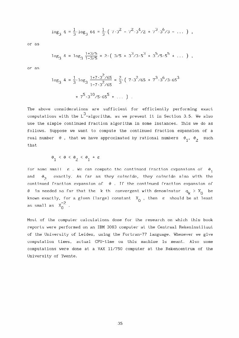
1 1 ( 2 2 4 3 6 )log 4 = -----Wlog 64 = -----W 7W3 - 7 W3 /2 + 7 W3 /3 - ... ,

3 3 3 3 9 0

or as

1+3/5 ( 3 3 5 5 )log 4 = log ------------------------- = 2W 3/5 + 3 /3W5 + 3 /5W5 + ... ,

3 3 1-3/5 9 0

or as

21 1+7W3 /65 2 ( 2 3 6 3

log 4 = -----Wlog --------------------------------------------- = -----W 7W3 /65 + 7 W3 /3W653 3 3 2 3 9

1-7W3 /65

5 10 5 )+ 7 W3 /5W65 + ... .

0

The above considerations are sufficient for efficiently performing exact3

computations with the L -algorithm, as we present it in Section 3.5. We also

use the simple continued fraction algorithm in some instances. This we do as

follows. Suppose we want to compute the continued fraction expansion of a

real number y , that we have approximated by rational numbers y , y such1 2

that

y < y < y < y + e1 2 1

for some small e . We can compute the continued fraction expansions of y1

and y exactly. As far as they coincide, they coincide also with the2

continued fraction expansion of y . If the continued fraction expansion of

y is needed so far that the k th convergent with denominator q > X bek 0

known exactly, for a given (large) constant X , then e should be at least0

-2as small as X .

0

Most of the computer calculations done for the research on which this book

reports were performed on an IBM 3083 computer at the Centraal Rekeninstituut

of the University of Leiden, using the Fortran-77 language. Whenever we give

computation times, actual CPU-time on this machine is meant. Also some

computations were done at a VAX 11/750 computer at the Rekencentrum of the

University of Twente.

35

Chapter 3. Algorithms for diophantine approximation.

3.1. Introduction.

In this section we give details of the computational methods we use to reduce

upper bounds for the solutions of diophantine equations. Our starting point

will always be a linear form L that is close to 0 (in the real or p-adic

sense, with the word "close" defined explicitly in terms of an inequality

involving the unknowns), together with a large but explicitly known upper

bound for the absolute values of the coefficients of L . Our aim is to

reduce the upper bound by showing that there are no solutions between the new

and the old upper bound.

Let y , ..., y , b be given numbers, in R , or in W , for a fixed prime1 n p

p . Let x , ..., x be unknowns in Z . Put1 n

nL = b + S x Wy .

i ii=1

We classify such linear forms according to three criteria:

-----L homogeneous if b = 0 , inhomogeneous if b $ 0 ;

-----L one-dimensional if n = 2 , multi-dimensional if n > 3 ;

-----L real if y e R for all i , p-adic if y e W for all i .i i p

The reason that the case n = 2 is called one-dimensional is that in the

homogeneous case the linear form

L = x Wy + x Wy1 1 2 2

leads to studying the simple, one-dimensional continued fraction expansion of

-y /y . The inhomogeneous case with n = 1 , viz.1 2

L = b + xWy

is not of any interest in the real case, but it is of interest in the p-adic

case. We call this the zero-dimensional case.

36

In the p-adic case we require that the quotients y /y and b/y are ini j j

Q itself, whereas the numbers y , b are allowed to be in some largerp isubfield of W .

p

Let c, d be positive constants. Put X = max|x | . Let X be a (large)i 0

positive constant. In the real case we shall always assume that

|L| < cWexp(-dWX) , (3.1)

X < X . (3.2)0

Let c , c be real constants, with c > 0 . In the p-adic case we shall1 2 2

assume that x > 0 for some index j e {1,...,n} , andj

ord (L) > c + c Wx , (3.3)p 1 2 j

X < X . (3.4)0

Our aim is to find a constant X , of the size of log X , such that in the1 0

real case (3.2) can be replaced by X < X , and in the p-adic case the bound1

x < X (a consequence of (3.4)) can be improved to x < X .j 0 j 1

In the forthcoming sections we will treat all cases, according to the3

classification given above. We insert Sections 3.4, 3.5 on the L -algorithm,

which will be our main computational tool, Section 3.6 on finding short

vectors in lattices, and Section 3.13 on certain sublattices that are useful

for our applications.

3.2. Homogeneous one-dimensional approximation in the real case: continued

fractions.

We first study the case

L = x Wy + x Wy .1 1 2 2

Put y = -y /y . We assume that y is irrational. Let the continued1 2

fraction expansion of y be given by

y = [ a , a , a , .... ] ,0 1 2

and let the convergents p /q for n = 0, 1, 2, ... be defined byn n

37

& p = 1 , p = a , p = a Wp + p-1 0 0 n+1 n+1 n n-1

{ .7 q = 0 , q = 1 , q = a Wq + q

-1 0 n+1 n+1 n n-1

It is well known that the convergents satisfy the inequalities

p1 n 1

------------------------------------------------------- < | y - ---------- | < ----------------------------------- , (3.5)2 q 2

(a +2)Wq n a Wqn+1 n n+1 n

and that if p/q satisfies the inequality

p 1| y - ----- | < -------------------- , (3.6)

q 22Wq

then p/q must be one of the convergents (cf. Hardy and Wright [1979],

Theorems 163, 171 and 184).

We may assume without loss of generality that |y | < |y | , that x > 0 ,1 2 1

*and that (x ,x ) = 1 . From (3.1) it follows that there exists a number X

1 2*

such that X > X implies X = x and (3.6) for (p,q) = (-x ,x ) . We now1 2 1

have the following criteria.

*LEMMA_3.1. (i). If (3.1) and (3.2) hold for x , x with X > X , then

1 2(-x ,x ) = (p ,q ) for an index k that satisfies

2 1 k k

( ) (1 )k < -1 + log r5WX +1 /log -----(1+r5) . (3.7)

9 0 0 92 0

Moreover, the partial quotient a satisfiesk+1

-1a > -2 + |y |Wc Wexp(dWq )/q . (3.8)k+1 2 k k

*(ii). If for some k with q > X

k

-1a > |y |Wc Wexp(dWq )/q , (3.9)k+1 2 k k

then (3.1) holds for (-x ,x ) = (p ,q ) .2 1 k k

*Proof. (i). By X > X and (3.6) it follows that (-x ,x ) = (p ,q ) for

2 1 k kan index k . Since q is at least the (k+1) th Fibonacci number, (3.7)

kfollows from q = x = X < X . To prove (3.8), apply (3.1) and the first

k 1 0inequality of (3.5).

(ii). Combine (3.9) with the second inequality of (3.5). p

38

We may apply Lemma 3.1(i) directly, or as follows.

LEMMA_3.2. Let

A = max(a ) ,k+1

where the maximum is taken over all indices k satisfying (3.7). If (3.1)

and (3.2) hold for x , x with X > X , then1 2 1

1 ( ) 1X < -----Wlog cW(A+2)/|y | + -----Wlog X .

d 9 2 0 d

Remark. From Lemma 3.2 an upper bound for X follows. We can apply Lemma

2.1 here, but Lemma 2.1 is sharp for large b only.

Proof. (3.1) and (3.5) yield

2 -1(a +2)Wq > q W|y |/|L| > q W|y |Wc Wexp(dWX) .n+1 n n 2 n 2

The result follows by applying Lemma 3.1(i). p

In practice it does not often occur that A is large. Therefore this lemma

is useful indeed.

Summarizing, this case comes down to computing the continued fraction of a

real number to a certain precision, and establishing that it has no extremely

large partial quotients. This idea has been applied in practice by Ellisonb

[1971 ], by Cijsouw, Korlaar and Tijdeman (appendix to Stroeker and Tijdeman

[1982]), and by Hunt and van der Poorten (unpublished) for solving

diophantine equations, by Steiner [1977] in connection with the Syracuse

("3WN+1") problem, and by Cherubini and Walliser [1987] (using a small home

computer only) for determining all imaginary quadratic number fields with

class number 1. We shall use it in Chapters 4 and 5.

3.3. Inhomogeneous one-dimensional approximation in the real case: the

Davenport lemma.

The next case is when L has the form

L = b + x Wy + x Wy ,1 1 2 2

39

where b $ 0 . We then may use the so-called Davenport lemma, which was

introduced by Baker and Davenport [1969]. It is, like the homogeneous case,

based on the continued fraction algorithm.

Put again y = -y /y , and put j = b/y . Then we have1 2 2

L---------- = j - x Wy + x .y 1 22

Let p/q be a convergent of y with q > X . We have the following result.0

LEMMA_3.3._(Davenport). Suppose that, in the above notation,

NqWjN > 2WX /q , (3.10)0

(by NWN we denote the distance to the nearest integer). Then the solutions

of (3.1), (3.2) satisfy

1 ( 2 )X < -----Wlog q Wc/|y |WX . (3.11)

d 9 2 00

Proof. From (3.5) and (3.10) we infer

2WX /q < NqW(j-x Wy+x )+x W(qWy-p)N < qW|L/y | + |x |/q .0 1 2 1 2 1

By (3.1), (3.2), and

2 -1X < q WcW|y |Wexp(-dWX) ,0 2

this leads to (3.11). p

If (3.10) is not true for the first convergent with denominator > X , then0

one should try some further convergents. If q is not essentially larger

than X , then (3.11) yields a reduced upper bound for X of size log X ,0 0

as desired. If no q of the size of X can be found that also satisfies0

(3.10) (a situation which is very unlikely to occur, as experiments show),

then not all is lost, since then only very few exceptional possible solutions

have to be checked. See Baker and Davenport [1969] for details.

Summarizing, we see that in this case the essential idea is that an extremely

large solution of (3.1) and (3.2) leads to a large range of convergents p/q

of y for which the values of NqWjN are all extremely small. In practice

it appears to be the case that qWj is always far enough from the nearest

40

integer (the values of NqWjN seem to be distributed randomly over the

interval [0,0.5] ). This method has been used in practice by Baker and

Davenport [1969] as we already mentioned, by Ellison, Ellison, Pesek, Stahl

and Stall [1972], by Steiner [1986], and by Gasl [1988]. We shall use it in

Chapter 4. Note that the method that we develop in Section 3.8 for the

multi-dimensional inhomogeneous case, can be used in the one-dimensional caseb

as well, as has been demonstrated in de Weger [1989 ].

33.4. The L -lattice basis reduction algorithm, theory.

To deal with linear forms with n > 3 , a straightforward generalization of

the case n = 2 would be to study multi-dimensional continued fractions. For

a good survey of this field, see Brentjes [1981]. However, the available

algorithms in this field seem not to have the desired efficiency and

generality. Fortunately, since 1981 there is a useful alternative, which in a

sense is also a generalization of the one-dimensional continued fraction

algorithm.

In 1981, L. Lovssz invented an algorithm, that has since then become known as3

the L -algorithm. It has been published in Lenstra, Lenstra and Lovssz

[1982], Fig. 1, p. 521. Throughout this and the next section we refer to this

paper as "LLL". The algorithm computes from an arbitrary basis of a latticen

in R another basis of this lattice, a so-called reduced basis, which has

certain nice properties (its vectors are nearly orthogonal).

The algorithm has many important applications in a variety of mathematical

fields, such as the factorization of polynomials (LLL, Lenstra [1984]),

public-key cryptography (Lagarias and Odlyzko [1985]), and the disproof of

the Mertens Conjecture (Odlyzko and te Riele [1985]). Of interest to us are

its applications to diophantine approximation, which already had been noticed

in LLL, p. 525. The algorithm has a very good theoretical complexity

(polynomial-time in the length of the input parameters), and performs also

very well in practical computations.

nLet G C R be a lattice, that is given by the basis b , ..., b . We

1 nintroduce the concept of a reduced basis of G , according to LLL, p. 516.

*The vectors b (for i = 1, ..., n ) and the real numbers m (for

i i,j1 < j < i < n ) are inductively defined by

41

i-1* * * * *b = b - S m Wb , m = (b ,b ) / (b ,b ) .i i i,j j i,j i j j j

j=1

* * nThen b , ..., b is an orthogonal basis of R . We call the lattice basis

1 nb , ..., b of G reduced if1 n

1|m | < ----- for 1 < j -----W|b | for 1 2 W|b | for i = 1, ..., n . (3.12)i 1

We remark that a lattice may have more than one reduced basis, and that the3

ordering of the basis vectors is not arbitrary. The L -algorithm accepts as

input any basis b , ..., b of G , and it computes a reduced basis1 n

c , ..., c of that lattice. The properties of reduced bases that are of1 n

nmost interest to us are the following. Let y e R be a given point, that is

not a lattice point. We denote by l(G) the length of the shortest non-zero

vector in the lattice, viz.

l(G) = min |x| ,0$xeG

and by l(G,y) the distance from y to the nearest lattice point, viz.

l(G,y) = min|x-y| .xeG

From a reduced basis lower bounds for both l(G) and l(G,y) can be

computed, according to the following results. Lemma 3.4 is Proposition (1.11)

from LLL. We recall its proof here, to show the similarity of the proofs of

Lemma’s 3.4 and 3.5.

LEMMA_3.4._(Lenstra,_Lenstra_and_Lovasz_[1982]). Let c , ..., c be a1 n

reduced basis of the lattice G . Then

-(n-1)/2l(G) > 2 W|c | .

1

Proof. Let 0 $ x e G be the lattice point with minimal length

|x| = l(G) . Write

42

n n* *

x = S r Wc = S r Wb ,i i i i

i=1 i=1

*with r e Z , r e R . Let i be the largest index such that r $ 0 .

i i 0 i0

* *Then, since c , ..., c span the same linear space as b , ..., b for all

1 i 1 i*

i , and b is the projection of c on the orthogonal complement ofi+1 i+1

*this linear space, it follows that r = r . Hence, by (3.12),

i i0 0

i0

2 2 *2 * 2 *2 * 2 2 * 2l(G) = |x| = S r W|b | > r W|b | = r W|b |

i i i i i ii=1 0 0 0 0

* 2 -(n-1) 2> |b | > 2 W|c | . p

i 10

LEMMA_3.5. Let c , ..., c be a reduced basis of the lattice G , and let1 n

ny = S s Wc for s , ..., s e R , with not all s in Z . Let i be

i i 1 n i 0i=1

the largest index such that s m Z . Theni0

-(n-1)/2l(G,y) > 2 WNs NW|c | .

i 10

Proof. Let x e G be the lattice point nearest to y . So |x-y| = l(G,y) .

Write

n n n n* * * *

x = S r Wc = S r Wb , y = S s Wc = S s Wb ,i i i i i i i i

i=1 i=1 i=1 i=1

* *with r e Z , r , s , s e R . Let i be the largest index such that

i i i i 1r $ s . Then, reasoning as in the proof of Lemma 3.4, we findi i1 1

* *r - s = r - s .i i i i1 1 1 1

Using (3.12) it follows that

2 2 * 2 2 -(n-1) 2l(G,y) > (r -s ) W|b | > (r -s ) W2 W|c | .

i i i i i 11 1 1 1 1

Obviously, i > i . If i = i the result follows at once. If i > i1 0 1 0 1 0

then s e Z , s $ r , hence |r -s | > 1 , and the result follows. pi i i i i1 1 1 1 1

The above lemma is rather weak in the extraordinary situation that s isi0

43

extremely close to an integer. If one of the other s is not close to ani

integer, we can apply the following variant.

LEMMA_3.6. Let c , ..., c be a reduced basis of the lattice G , and let1 n

ny = S s Wc for s , ..., s e R , with not all s in Z . Suppose that

i i 1 n ii=1

1there is an index i and constants d , 0 < d < ----- such that

0 1 2 2

Ns N < d for i = i +1, ..., n ,i 1 0

Ns N > d .i 20

Then

-(n-1)/2l(G,y) > 2 Wd W|c | - (n-i )Wd Wmax |c | .

2 1 0 1 ii>i

0

Proof. With notation as in the proof of Lemma 3.5, let t be the integeri

nearest to s , for i > i + 1 , and t = s for i |x-z| - |z-y| .

Now,

n|z-y| < S |s -t |W|c | < (n-i )Wd Wmax |c | ,

i i i 0 1 ii=i +1 i>i

0 0

and, using (3.12),

n2 * * 2 * 2 * * 2 * 2

|x-z| = S (r -t ) W|b | > (r -t ) W|b |i i i i i i

i=1 1 1 1

2 -(n-1) 2> (r -t ) W2 W|c | .

i i 11 1

Obviously, i > i . If i = i the result follows. If i > i then1 0 1 0 1 0

44

t e Z, t $ r , hence |r -t | > 1 > d , and the result follows. pi i i i i 21 1 1 1 1

3Remark. Babai [1986] showed that the L -algorithm can be used to find a

lattice point x with |x-y| < cWl(G,y) for a constant c depending on the

dimension of the lattice only. This result can also be used instead of Lemma

3.5 or 3.6.

33.5. The L -lattice basis reduction algorithm, practice.

3Below (in Fig. 1) we describe the variant of the L -algorithm that we use in

this monograph to solve diophantine equations. This variant has been designed

to work with integers only, so that rounding-off errors are avoided

completely. In the algorithm as stated in LLL, Fig. 1, p. 521, non-integral

rational numbers may occur, even if the input parameters are all integers.

n *Let G C Z be a lattice with basis vectors b , ..., b . Define b , m ,

1 n i ijd as in LLL (1.2), (1.3), (1.24), respectively. The d can be used asi idenominators for all numbers that appear in the original algorithm (LLL, p.

523). Thus, put for all relevant indices i, j

*c = d Wb ,i i-1 i

(3.13)

l = d Wm .i,j j i,j

* 2They are integral, by LLL (1.28), (1.29). Notice that, with B = |b | ,

i i

d = d WB . (3.14)i i-1 i

*We can now rewrite the algorithm in terms of c , d , l in stead of b ,

i i i,j iB , m , thus eliminating all non-integral rationals. We give this varianti i,j

3of the L -algorithm in Fig. 1. All the lines in this variant are evident from

applying (3.13) and (3.14) to the corresponding lines in the original

algorithm, except the lines (A), (B) and (C), which will be explained below.

We added a few lines to the algorithm, in order to compute the matrix of the

transformation from the initial to the reduced basis. Let B be the matrix

with column vectors b , ..., b , the initial basis of the lattice G ,1 n

which is the input for the algorithm. We say: B is the matrix associated to

the basis b , ..., b . Let C be the matrix associated to the reduced1 n

45

u---------------------------------------------------------------------------------------------------------------------------------------------------------------------------------------------------------------------------------------------------------------------------------------------------------------------------------------------------------------------------------------o1

1 11 d := 1 ;

0 11 )

11 c := b ; |

i i 11 ) |

11 l := (b ,c ) ; | |

i,j i j 11 } for j=1,...,i-1 ; } for i=1,...,n ;

11 (A) c := (d Wc -l Wc )/d | |

i j i i,j j j-1 11 0 |

11 d := (c ,c )/d |

i i i i-1 11 0

11

k := 2 ; 11

11

(1) perform (*) for l = k-1 ; 11

11 2 2

if 4Wd Wd < 3Wd - 4Wl go to (2) ; 11 k-2 k k-1 k,k-1

11

perform (*) for l = k-2, ..., 1 ; 11

11

if k = n terminate ; 11

11

k := k+1 ; go to (1) ; 11

11

& b * & b * 11 k-1 k

(2) | | := | | ; 11 b b

7 k 8 7 k-1 8 11

11 T T

& u * & u * & v’ * & v’ * 11 k-1 k k-1 k

| | := | | ; | | := | | ; 11 u u T T

7 k 8 7 k-1 8 7 v’ 8 7 v’ 8 11 k k-1

11

& l * & l * 11 k-1,j k,j

| | := | | for j = 1, ..., k-2 ; 11 l l

7 k,j 8 7 k-1,j 8 11

11

& l * & l * & d * 11 i,k-1 k,k-1 k-2(B) | | := ( l W| | + l W| | ) / d 1

1 l i,k-1 d i,k -l k-17 i,k 8 7 k 8 7 k,k-1 8 1

11

1 for i = k+1, ..., n ;1

12 1

1 (C) d := ( d Wd + l ) / d ;k-1 k-2 k k,k-1 k-1 1

11

1 if k > 2 then k := k-1 ;1

11

1 go to (1) ;1

11

1 (*) if 2W|l | > d thenk,l l 1

11

1 & r := integer nearest to l /d ;k,l l 1

1 |T T T 1

1 | b := b - rWb ; u := u - rWu ; v’ := v’ + rWv’ ;k k l k k l l l k 1

1 {1

1 | l := l - rWl for j = 1, ..., l-1 ;k,j k,j l,j 1

1 |1

1 7 l := l - rWd .k,l k,l l 1

1m---------------------------------------------------------------------------------------------------------------------------------------------------------------------------------------------------------------------------------------------------------------------------------------------------------------------------------------------------------------------------------------.

3Figure_1. Variant of the L -algorithm.

46

basis c , ..., c , which the algorithm delivers as output. Then we define1 n

this transformation matrix V by

C = BWV .

More generally, let U be the matrix of a transformation from some B to0

B , so B = B WU . Denote the column vectors of U by u , ..., u , and the0 1 n

-1 T Trow vectors of U by v’ , ..., v’ . We feed the algorithm with U and

1 n-1

U as well. All manipulations in the algorithm done on the b are alsoi

Tdone on the u , and the v’ are adjusted accordingly. This does not

i iaffect the computation time seriously. The algorithm now gives as output

-1matrices C , U’ and U’ , such that C is associated to a reduced basis,

C = BWV , and U’ = UWV . Note that V is not computed explicitly, unless

U = I (the unit matrix), in which case U’ = V . It follows that

-1C = BWU WU’ = B WU’ ,

0

so U’ is the matrix of the transformation from B to C . Note that if0

-1 -1B is known, then it is not much extra effort to compute C as well.0

We now explain why lines (A), (B) and (C) are correct.

(A): From LLL (1.2) it follows that

i-1 di-1

c = d Wb - S -----------------------------------Wl Wc .i i-1 i d Wd i,k k

k=1 k-1 k

Define for j = 0, 1, ..., i-1

j dj

c (j) = d Wb - S -----------------------------------Wl Wc .i j i d Wd i,k k

k=1 k-1 k

Then c (0) = b , and c (i-1) = c . The c (j) is exactly the vectori i i i i

computed in (A) at the j th step, since

d Wc (j-1) - l Wcj i i,j j

----------------------------------------------------------------------------------------------------dj-1

j-1 d dj j

= d Wb - S -----------------------------------Wl Wc - -----------------------------------Wl Wc = c (j) .j i d Wd i,k k d Wd i,j j i

k=1 k-1 k j-1 j

This explains the recursive formula in line (A). It remains to show that the

occurring vectors c (j) are integral. This follows fromi

47

j j1 *

d W S -----------------------------------Wl Wc = d W S m Wb ,j d Wd i,k k j i,k kk=1 k-1 k k=1

which is integral by LLL p. 523, l. 11.

(B), (C): Notice that the third and fourth line, starting from label (2), in

the original algorithm, are independent of the first, second and fifth line.

Thus a permutation of these lines is allowed. We rewrite the first, second

and fifth line as follows (where we indicate variables that have been changed

with a prime sign):

2B’ := B + m WB ; (3.15)k-1 k k,k-1 k-1

B’ := B WB /B’ ; (3.16)k k-1 k k-1

m’ := m WB /B’ ; (3.17)k,k-1 k,k-1 k-1 k-1

m’ := m’ Wm + (1-m Wm’ )Wm ; (3.18)i,k-1 k,k-1 i,k-1 k,k-1 k,k-1 i,k

m’ := m - m Wm ; (3.19)i,k i,k-1 k,k-1 i,k

where (3.18) and (3.19) hold for i = k+1, ..., n . The d remain unchangedi

for i = 0, 1, ..., k-2 , and by (3.16) also for i = k . Now, (3.15) is

equivalent to

2d’ d l dk-1 k k,k-1 k-1

-------------------- = -------------------- + ------------------------------ W -------------------- , (3.20)d d 2 dk-2 k-1 d k-2

k-1

which explains (C). From (3.17) we find

l’ l d d’k,k-1 k,k-1 k-1 k-2

------------------------------ = ------------------------------ W -------------------- W -------------------- ,d’ d d d’k-1 k-1 k-2 k-1

hence l remains unchanged. From (3.18) we obtaink,k-1

l’ l l l l li,k-1 k,k-1 i,k-1 & k,k-1 k,k-1 * i,k

------------------------------ = ------------------------------ W ------------------------------ + 1 - ------------------------------ W ------------------------------ W -------------------- ,d’ d’ d 7 d d’ 8 dk-1 k-1 k-1 k-1 k-1 k

whence, by multiplying by d Wd’ and using (3.20),k-1 k-1

l2 i,k

d Wl’ = l Wl + ( d Wd’ - l )W--------------------k-1 i,k-1 k,k-1 i,k-1 k-1 k-1 k,k-1 d

k

= l Wl + d Wl .k,k-1 i,k-1 k-2 i,k

48

Finally, from (3.19) we see

l’ l l li,k i,k-1 k,k-1 i,k

-------------------- = ------------------------------ - ------------------------------ W -------------------- ,d d d dk k-1 k-1 k

and (B) follows.

In our applications we often have a lattice G , of which a basis is given

such that the associated matrix, A say, has the special form

( )1

| |. o

| . |.

A = | o | ,1

| |7 Q ... Q Q 8

1 n-1 n

where the Q are large integers, that may have several hundreds of decimali

digits. We can compute a reduced basis of this lattice directly, using the3

matrix A itself as input for the L -algorithm. But it may save time and

space to split up the computation into several steps with increasing

accuracy, as follows.

Let k be a natural number (the number of steps), and let l be a natural

number such that the Q have about kWl (decimal) digits. Fori

i = 1, ..., n and j = 1, ..., k put

(j) lW(k-j)Q = [Q /10 ] ,i i

(j)and define J by

i

(j+1) l (j) (j)Q = 10 WQ + J .i i i

(j)Thus, the J are blocks of l consecutive digits of Q . Define for the

i irelevant j the n * n matrices

& 1 * & *| . o | | |

.| . | | o |

oA = | 1 | , D = | | ,j j

| | | |(j) (j) (j) (j) (j)

7 Q ... Q Q 8 7 J ... J 81 n-1 n 1 n

& 1 *. o

| . |.

E = | | .1

| o |l

7 10 8

49

Then it follows at once that

A = EWA + D .j+1 j j

(k)Notice that A = A , since Q = Q . Put U = I , B = A . For some

k i i 0 1 13

j > 1 let B and U be known matrices. Then we apply the L -algorithmj j-1

-1to B = B , U = U , and U . We thus find matrices C , U , and

j j-1 j j-1

U such thatj

-1C6 = B WU WU .j j j-1 j

Now put

B = EWC + D WU .j+1 j j j

By induction B , C and U are defined for j = 1, ..., k . Note thatj j j

-1 -1B WU = EWB6WU + D ,j+1 j j j-1 j

-1so the B WU satisfy the same recursive relation as the A . Since

j j-1 j-1 -1

B WU = A , we have B WU = A for all j . Hence1 0 1 j j-1 j

-1C = B WU WU6 = A WU ,j j j-1 j j j

and it follows that C and A are associated to bases of the samek k

3lattice, which is G . Moreover, since C is output of the L -algorithm, it

kis associated to a reduced basis of G .

Let us now analyse the computation time. For a matrix M we denote by L(M)3

the maximal number of (decimal) digits of its entries. If the L -algorithm is

applied to a matrix B , with as output a matrix C , then according to the

experiences of Lenstra, Odlyzko (cf. Lenstra [1984], p. 7) and ourselves, the3

computation time is proportional to L(B) in practice. Since C is

associated to a reduced basis, we assume that

10L(C) = log(det G)/n .

(j)In our situation, L(A ) = lWj , L(D ) = l , and by det C = det A = Q

j j j j n(j) (j)

we have L(C ) = lWj/n . Put C = (c ) , U = (u ) . Then byj j i,h j i,h

(j) (j)C = A WU and the special shape of A we have c = u forj j j j i,h i,h

i = 1, ..., n-1 and h = 1, ..., n , and

(j) ( (j) (j) (j) (j) (j) ) (j)u = - c WQ - ... - c WQ + c /Q .n,h 9 1,h 1 n-1,h n-1 n,h 0 n

50

It follows that L(U ) = L(C ) . Soj j

( )L(B ) = max L(EWC ), L(D WU ) = l + lW(j-1)/n .

j 9 j-1 j-1 j-1 0

3Instead of applying the L -algorithm once with A as input, we apply it k

times, with B , ..., B as input. Thus we reduce the computation time by a1 k

factor

3 3 3 3L(A) (lWk) k Wn

------------------------------------------------ = --------------------------------------------------------------------- = ---------------------------------------- .k k k-1

3 3 ( j-1)3 3S L(B ) S l W 1+--------------- S (n+j)

j 9 n 0j=1 j=1 j=0

2For k between 2.5Wn and 3Wn this expression is maximal, about 0.4Wn .

So the reduction in computation time is considerable (a factor 10 already for

n = 5 ). The storage space that is required is also reduced, since the( )

largest numbers that appear in the input have lW 1+(k-1)/n instead of lWk9 0

digits.

3.6. Finding all short lattice points: the Fincke and Pohst algorithm.

Sometimes it is not sufficient to have only a lower bound for l(G) or

l(G,y) . It may be useful to know exactly all vectors x e G such that

|x| < C or |x-y| < C for a given constant C . There exists an efficient

algorithm for finding all the solutions to these problems. This algorithm was

devised by Fincke and Pohst [1985], cf. their (2.8) and (2.12). We give a

description of this algorithm below.

The input of the algorithm is a matrix B whose column vectors span the

lattice G , and a constant C > 0 . The output is a list of all lattice

points x e G with |x| < C , apart from x = 0 . We give the algorithm in

Figure 2. We use the notation X = (x ) for matrices X = A, B, R, S, U ,ij

and x for the column vectors of X .i

The algorithm can also be used for finding all vectors x e G of which the

distance to a given non-lattice point y is at most a given constant C .

Namely, let

ny = S s Wb ,

i ii=1

and let r be the integer nearest to s for all i . Puti i

51

u-----------------------------------------------------------------------------------------------------------------------------------------------------------------------------------------------------------------------------------------------------------------------------------------------------------------------------------------------------------------------------------------------------------------o1 11 T 1

A := B WB ;1 11 q := a for 1 < i < j < n ; 1

ij i j1 1

q := q , q := q /q for 1 < i < j < n ;1 ji i j ij ij ii 11 q := q - q Wq for i+1 < k < l < n for 1 < i < n ; 1

kl k l ki il1 1

r := rq for 1 < i < n ;1 ii ii 11 r := r Wq , r := 0 for 1 < j < i < n ; 1

ij i i ij ji1 -1 1

compute R ;1 1

-1 -1 -11 compute a row-reduced version S of R , and U, U such 11 -1 -1 -1 1

that S = U WR ;1 11 compute S = RWU4; 11 1

determine a permutation p such that |s | > ... > |s | ,1 p(1) p(n) 11 let S’ be the matrix with columns s for i = 1,...,n ; 1

-11 p (i) 1

T1 A := S’ W S’ ; 11 1

q := a for 1 < i < j < n ;1 ij i j 11 q := q , q := q /q for 1 < i < j < n ; 1

ji i j ij ij ii1 1

q := q - q Wq for i+1 < k < l < n for 1 < i < n ;1 kl k l ki il 11 i := n ; 11 1

T := C ;1 i 11 U := 0 ; 1

i1 1

(1) Z := r(T /q ) ;1 i ii 11 UB(x ) := 3Z-U 4 ; 1

i i1 1

x := #-Z -U $ - 1 ;1 i i 11 (2) x := x + 1 ; 1

i i1 1

if x < UB(x ) , go to (4) ;1 i i 11 (3) i := i + 1 ; 11 1

go to (2) ;1 11 (4) if i = 1 , go to (5) ; 11 1

i := i - 1 ;1 1

m1 1

U := S q Wx ;1 i ij j 1

j=i +11 2 1

T := T - q W(x +U ) ;1 i i+ 1 i+1,i+1 i+1 i+1 11 go to (1) ; 11 1

(5) if x = 0 for 1 < i < n , terminate ;1 i 1

T1 compute a nd print x = UW(x ,...,x ) ; 1

-1 -11 p (1) p (n) 11 go to (2) . 11 1m-----------------------------------------------------------------------------------------------------------------------------------------------------------------------------------------------------------------------------------------------------------------------------------------------------------------------------------------------------------------------------------------------------------------.

Figure_2. The Fincke and Pohst Algorithm.

52

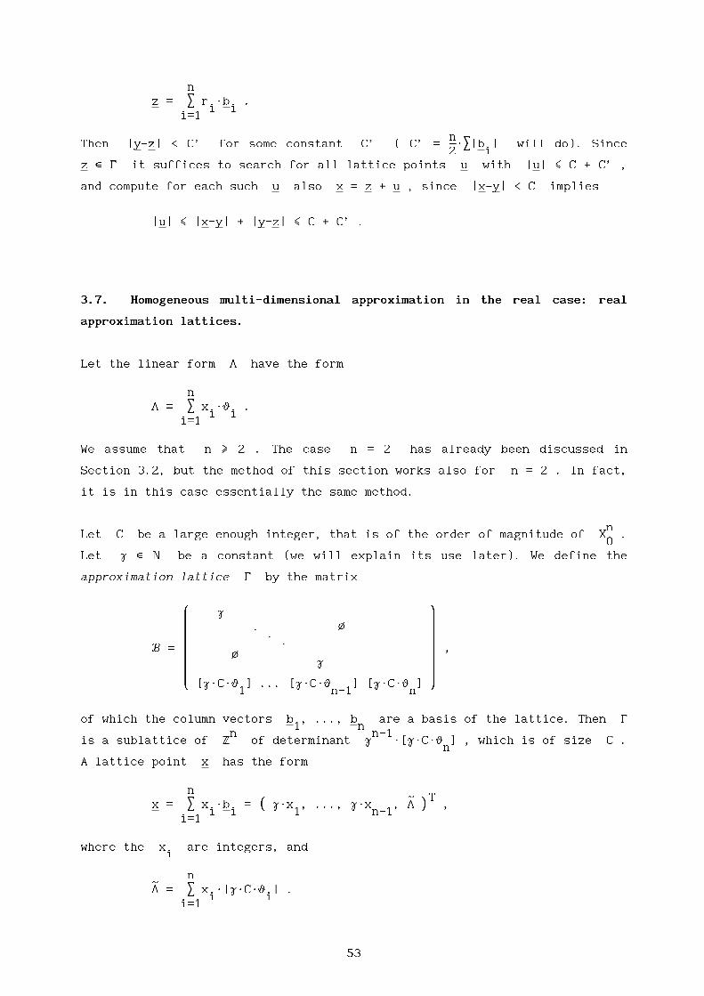
nz = S r Wb .

i ii=1

nThen |y-z| < C’ for some constant C’ ( C’ = -----WS|b | will do). Since

2 iz e G it suffices to search for all lattice points u with |u| < C + C’ ,

and compute for each such u also x = z + u , since |x-y| < C implies

|u| < |x-y| + |y-z| < C + C’ .

3.7. Homogeneous multi-dimensional approximation in the real case: real

approximation lattices.

Let the linear form L have the form

nL = S x Wy .

i ii=1

We assume that n > 2 . The case n = 2 has already been discussed in

Section 3.2, but the method of this section works also for n = 2 . In fact,

it is in this case essentially the same method.

nLet C be a large enough integer, that is of the order of magnitude of X .

0Let g e N be a constant (we will explain its use later). We define the

approximation lattice G by the matrix

( )g

| |. o

| . |.

B = | | ,o

| g || |[gWCWy ] ... [gWCWy ] [gWCWy ]

9 1 n-1 n 0

of which the column vectors b , ..., b are a basis of the lattice. Then G1 n

n n-1is a sublattice of Z of determinant g W[gWCWy ] , which is of size C .

nA lattice point x has the form

n( ~ )T

x = S x Wb = gWx , ..., gWx , L ,i i 9 1 n-1 0

i=1

where the x are integers, andi

n~L = S x W[gWCWy ] .

i ii=1

53

~Clearly, L is close to gWCWL . The length of the vector x now measures

both X and |L| , which are exactly the two numbers we want to balance0

with each other. Heuristics (cf. Section 1.3) tell us that in a generic case-n

we expect |L| = X . We now can prove easily the following useful lemma.0

LEMMA_3.7. Let X be a positive number such that1

( 2 2)l(G) > r (n+1) +(n-1)Wg WX . (3.21)

9 0 1

Then (3.1) has no solutions with

1-----Wlog(gWCWc/X ) < X < X . (3.22)d 1 1

Remark. We apply this lemma for X = X . If condition (3.21) then fails,1 0

we must take a larger constant C . If it holds for a constant C of then

size X , then (3.22) yields a reduced lower bound for X of size log X .0 0

Proof. Let x , ..., x be a solution of (3.1) with 0 < X < X . Consider1 n 1

the lattice point

n( ~ )T

x = S x Wb = gWx , ..., gWx , L ,i i 9 1 n-1 0

i=1

~with L as above. Then

n-12 2 2 ~2 2 2 ~2

|x| = g W S x + L < (n-1)Wg WX + L ,i 1

i=1

and

n n~|L-gWCWL| < S |x |W|[gWCWy ]-gWCWy | < S |x | , (3.23)

i i i ii=1 i=1

which is < nWX . By (3.1), (3.21) and the definition of l(G) we have1

~ ~gWCWcWexp(-dWX) > |gWCWL| > |L| - |L-gWCWL|

( 2 2 2)> r l(G) -(n-1)Wg WX - nWX > X ,

9 10 1 1

and (3.22) follows at once. p

Condition (3.21) can be checked by computing a reduced basis of the lattice3

G by the L -algorithm, and applying Lemma 3.4. The parameter g is used to

keep the "rounding-off error"

54

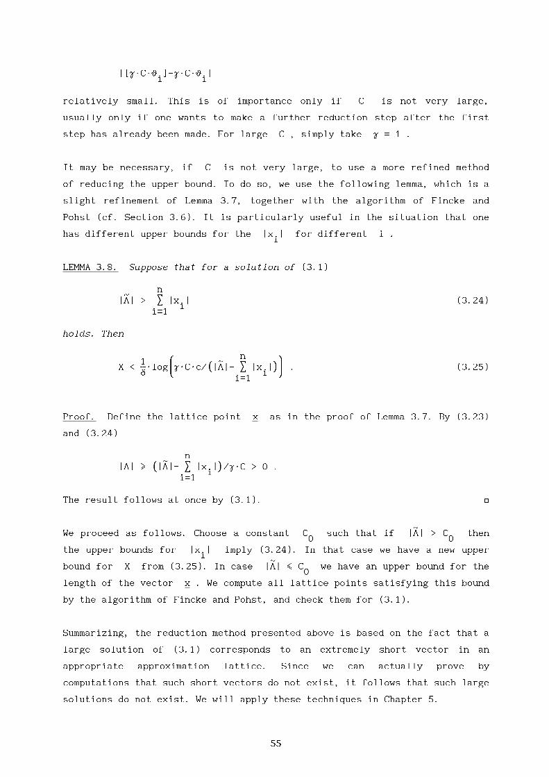
|[gWCWy ]-gWCWy |i i

relatively small. This is of importance only if C is not very large,

usually only if one wants to make a further reduction step after the first

step has already been made. For large C , simply take g = 1 .

It may be necessary, if C is not very large, to use a more refined method

of reducing the upper bound. To do so, we use the following lemma, which is a

slight refinement of Lemma 3.7, together with the algorithm of Fincke and

Pohst (cf. Section 3.6). It is particularly useful in the situation that one

has different upper bounds for the |x | for different i .i

LEMMA_3.8. Suppose that for a solution of (3.1)

n~|L| > S |x | (3.24)

ii=1

holds. Then

n1 & ( ~ )*

X < -----Wlog gWCWc/ |L|- S |x | . (3.25)d 7 9 i 08

i=1

Proof. Define the lattice point x as in the proof of Lemma 3.7. By (3.23)

and (3.24)

n( ~ )

|L| > |L|- S |x | /gWC > 0 .9 i 0

i=1

The result follows at once by (3.1). p

~We proceed as follows. Choose a constant C such that if |L| > C then

0 0the upper bounds for |x | imply (3.24). In that case we have a new upper

i~

bound for X from (3.25). In case |L| < C we have an upper bound for the0

length of the vector x . We compute all lattice points satisfying this bound

by the algorithm of Fincke and Pohst, and check them for (3.1).

Summarizing, the reduction method presented above is based on the fact that a

large solution of (3.1) corresponds to an extremely short vector in an

appropriate approximation lattice. Since we can actually prove by

computations that such short vectors do not exist, it follows that such large

solutions do not exist. We will apply these techniques in Chapter 5.

55

3.8. Inhomogeneous multi-dimensional approximation in the real case: an

alternative for the generalized Davenport lemma.

Let L be the most general linear form that we will study, viz.

nL = b + S x Wy ,

i ii=1

where n > 2 (the case n = 2 has been dealt with in Section 3.3, but can

be incorporated here also). To deal with this inhomogeneous case, two methods

are available. The first method is a generalization of the method of

Davenport that we discussed in Section 3.3. The second method is closer to

the homogeneous case of the previous section.

First we explain briefly the generalized Davenport method. See Ellisona

[1971 ] (where only the case n = 3 is treated). Put

y’ = y /y for i = 1, ..., n-1 , b’ = b/y ,i i n n

n-1L’ = L/y = b’ + S x Wy’ + x .

n i i ni=1

Let (p ,...,p ,q) be a simultaneous approximation to y’, ..., y’ with1 n-1 1 n-1

n-1q of the size of X , such that, for i = 1, ..., n-1 ,

0

1+1/(n-1)|y’-p /q| < c’/qi i

for a small constant c’ .

LEMMA_3.9._(Davenport,_Ellison). Suppose that

1/(n-1)NqWb’N > 2W(n-1)WX Wc’/q .

0

Then the solutions of (3.1), (3.2) satisfy

1 ( 1+1/(n-1) )X < -----Wlog q Wc/|y |Wc’W(n-1)WX .

d 9 n 00

Proof. The result follows at once from

n-1NqWb’N < |qWL’+ S x W(p -qWy’)| <

i i ii=1

-1 1/(n-1)qW|y | WcWexp(-dWX) + (n-1)WX Wc’/q . p

n 0

56

To apply this generalized Davenport method in practice, it is necessary to

compute the simultaneous approximations (p ,...,p ,q) . We indicated in1 n-13

Section 1.4 how this can be done with the L -algorithm. As lattice we take

the one associated to the following matrix:

& 1 *| o |

[CWy’] -C| .1 . | ,

. .| . . |

o7 [CWy’ ] -C 8

n-1n

where C is a constant of size X . Then c , the first basis vector of a0 1

(n-1)/n n-1reduced basis, will have length of the size of C = X . But c

0 1can be written as

( )Tc = q, qW[CWy’]-CWp , ..., qW[CWy’ ]-C.p1 9 1 1 n-1 n-1 0

n-1for some p , ..., p , q . It is expected that q is of size X , and

1 n-1 0

qWCW|y’-p /q| = |qW[CWy’]-CWp |i i i i

n-1are of the size X , so that |y’-p /q| are of the size

0 i i

n-1 n-1 -1 -n -(1+1/(n-1))X /CWX = C = X = q ,0 0 0

as desired.

The above method has been applied in practice to solve Thue and Thue-Mahler

equations by Agrawal, Coates, Hunt and van der Poorten [1980] (using multi-3

dimensional continued fractions instead of the L -algorithm), Petho anda b

Schulenberg [1987], and Blass, Glass, Meronk and Steiner [1987 ], [1987 ]. So

it has proved to be useful. However, we prefer another method, for several

reasons. Firstly, it is close to the homogeneous case as described in the

previous section, whereas the generalized Davenport method has no obvious

counterpart for the homogeneous case. Secondly, it actually produces

solutions for which the linear form L is almost as near to zero as possible

under the condition X < X . Specifically, if a linear relation between the0

y exists, but had not been noticed before (a situation that may occur inipractice, cf. Agrawal, Coates, Hunt and van der Poorten [1980]), the method

detects these relations, by finding explicitly an extremely short lattice

vector (resp. a lattice vector extremely near to a given point) giving the

coefficients of the relation. Thirdly, an analogous method for the p-adic

case can be given (see Section 3.11). Finally, variations as indicated in

Section 1.4 are possible. Concerning computation time we think that the two

57

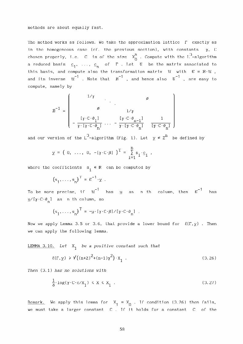
methods are about equally fast.

The method works as follows. We take the approximation lattice G exactly as

in the homogeneous case (cf. the previous section), with constants g, Cn 3

chosen properly, i.e. C is of the size X . Compute with the L -algorithm0

a reduced basis c , ..., c of G . Let C be the matrix associated to1 n

this basis, and compute also the transformation matrix U with C = BWU ,-1 -1 -1

and its inverse U . Note that B , and hence also C , are easy to

compute, namely by

& 1/g *. o

| . |.

| |-1 o

B = | 1/g || |

[gWCWy ] [gWCWy ] 1| 1 n-1 |- -------------------------------------------------- ... - -------------------------------------------------- ----------------------------------------

7 gW[gWCWy ] gW[gWCWy ] [gWCWy ] 8n n n

3 nand our version of the L -algorithm (Fig. 1). Let y e Z be defined by

n( )T

y = 0, ..., 0, -[gWCWb] = S s Wc ,9 0 i i

i=1

where the coefficients s e R can be computed byi

( )T -1s ,...,s = C Wy .9 1 n0

-1 -1To be more precise, if U has u as n th column, then C has

u/[gWCWy ] as n th column, son

( )Ts ,...,s = -uW[gWCWb]/[gWCWy ] .9 1 n0 n

Now we apply Lemma 3.5 or 3.6, that provide a lower bound for l(G,y) . Then

we can apply the following lemma.

LEMMA_3.10. Let X be a positive constant such that1

( 2 2)l(G,y) > r (n+2) +(n-1)g WX . (3.26)

9 0 1


1-----Wlog(gWCWc/X ) < X < X . (3.27)d 1 1

Remark. We apply this lemma for X = X . If condition (3.26) then fails,1 0

we must take a larger constant C . If it holds for a constant C of the

58

nsize X , then (3.27) yields a reduced lower bound for X of size log X .

0 0

Proof. Let x , ..., x be a solution of (3.1) with 0 < X < X . Consider1 n 1

the lattice point

n( ~ )T

x = S x Wb = gWx , ..., gWx , L ,i i 9 1 n-1 0 0

i=1

with

n~L = S x W[gWCWy ] .0 i i

i=1

~ ~Put L = [gWCWb] + L . Then

0

n-12 2 2 ~2 2 2 ~2

|x-y| = g W S x + L < (n-1)Wg WX + L ,i 1

i=1

and

n~|L-gWCWL| < |[gWCWb]-gWCWb| + S |x |W|[gWCWy ]-gWCWy |

i i ii=1

n< 1 + S |x | < 1 + nWX < (n+1)WX .

i 1 1i=1

By (3.1), (3.26) and the definition of l(G,y) the result follows, since

~ ~gWCWcWexp(-dWX) > |gWCWL| > |L| - |L-gWCWL|

( 2 2 2)> r l(G,y) -(n-1)Wg WX - (n+1)WX > X . p

9 10 1 1

Again we may prove refinements of the above lemma, similar to Lemma 3.8 in

the homogeneous case. We explained in Section 3.5. how to apply the Fincke

and Pohst algorithm in the inhomogeneous case. We do not work that out here.

Summarizing, the method described above is based on the fact that a large

solution of (3.1) in the inhomogeneous case leads to a lattice pointn

extremely near to a fixed point in Z . We can actually prove by some

computations that such lattice points do not exist, so that such extreme

solutions do not exist. The method outlined in this section is used in

Chapter 8. Note that in the case n = 2 the method is essentially the same

as the Davenport lemma.

59

3.9. Inhomogeneous zero-dimensional approximation in the p-adic case.

In the p-adic case we start with a very simple linear form L , to which also

a very simple reduction method applies. Let L be

L = b + xWy ,

for b, y e W such that b/y e Q , and x e Z , x > 0 . It is obviousp p

that in the real case with such a simple linear form L inequality (3.1) has

only finitely many solutions (we even don’t need (3.2)), that are easy to

compute. In the p-adic case however, inequality (3.3) may have infinitely

many solutions, so we do need a bound like (3.4), and a reduction method.

Put y’ = -b/y . Then y’ e Q . Inequality (3.3) now becomesp

ord (y’-x) > c’ + c Wx , (3.28)p 1 2

where c’, c are constants with c > 0 . We assume that1 2 2

x > -c’/c .1 2

Then (3.28) has no solutions if ord (y’) < 0 . Hence we may assume that y’p

is a p-adic integer. Let the p-adic expansion of y’ be

8i

y’ = S u Wp ,i

i=0

where u e { 0, 1, ..., p-1 } for all i e N . Compute the p-adic digitsi 0

u far enough to be able to apply the following reduction lemma.i

LEMMA_3.11. Let X be a positive constant. Let r be the minimal index1

such that

rp > X , u $ 0 . (3.29)

1 r


(r-c’)/c < x < X . (3.30)1 2 1

Remark. We apply the lemma with X = X . The assumption behind the lemma1 0

is that in the p-adic expansion of y’ no long sequences of zeroes appear.

In fact, it seems that in our applications the numbers u are distributedi

randomly over { 0, 1, ..., p-1 } . Then the minimal r satisfying (3.29)

60

will not be much larger than log X /log p , and then (3.30) yields a reduced0

upper bound of size log X , as desired.0

Proof. Let x < X satisfy (3.28). Suppose that ord (y’-x) > r + 1 . Then1 p

ri r+1

x _ S u Wp (mod p ) .i

i=0

By x > 0 it follows from (3.29) that

ri r r

x > S u Wp > u Wp > p > X ,i r 1

i=0

which contradicts the assumption x < X . Hence ord (y’-x) < r , and (3.30)1 p

follows from (3.28). p

Remark. In the above proof it is essential that x > 0 . It is however not

difficult to formulate a similar result that holds for all x e Z , by

looking, if p $ 2 for p-adic digits u that are not only $ 0 but alsoi

$ p-1 , and if p = 2 for p-adic digits u , u with u $ u .i i+1 i i+1

A method very similar to the one described above was used by Wagstaff [1979],n n

[1981], a.o. for solving 5 _ 2 (mod 3 ) . We apply the method in Chapter 4.

3.10. Homogeneous one-dimensional approximation in the p-adic case: p-adic

continued fractions and approximation lattices of p-adic numbers.

Let L have the form

L = x Wy + x Wy ,1 1 2 2

where y , y e W such that y = -y /y e Q , and x , x e Z . We may1 2 p 1 2 p 1 2

assume that ord (y) > 0 . Nowp

L’ = L/y = - x Wy + x .1 1 2

So (3.3) now means that the rational number x /x is p-adically close to2 1

the p-adic number y .

In analogy of the real case it seems reasonable to study p-adic continued

fraction algorithms. However, a p-adic continued fraction algorithm that

provides all best approximations to a p-adic number seems not to exist.

61

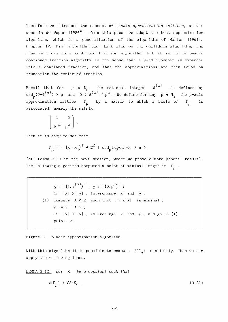
Therefore we introduce the concept of p-adic approximation lattices, as wasa

done in de Weger [1986 ]. From this paper we adopt the best approximation

algorithm, which is a generalization of the algorithm of Mahler [1961],

Chapter IV. This algorithm goes back also on the euclidean algorithm, and

thus is close to a continued fraction algorithm. But it is not a p-adic

continued fraction algorithm in the sense that a p-adic number is expanded

into a continued fraction, and that the approximations are then found by

truncating the continued fraction.

(m)Recall that for m e N the rational integer y is defined by

0(m) (m) m

ord (y-y ) > m and 0 < y < p . We define for any m e N the p-adicp 0

approximation lattice G by a matrix to which a basis of G ism m

associated, namely the matrix

& 1 0 *| | .

(m) m7 y p 8

Then it is easy to see that

( )T 2G = { x ,x e Z | ord (x -x Wy) > m }m 9 1 20 p 2 1

(cf. Lemma 3.13 in the next section, where we prove a more general result).

The following algorithm computes a point of minimal length in G .m

u---------------------------------------------------------------------------------------------------------------------------------------------------------------------------------------------------------------------------------------------------------------------------------------------------------------------------------------------------------------------------------------o1 1

( (m))T ( m)T1 x := 1,y ; y := 0,p ; 1

9 0 9 01 1

if |x| > |y| , interchange x and y ;1 11 (1) compute K e Z such that |y-KWx| is minimal ; 11 1

y := y - KWx ;1 11 if |x| > |y| , interchange x and y , and go to (1) ; 11 1

print x .1 11 1m---------------------------------------------------------------------------------------------------------------------------------------------------------------------------------------------------------------------------------------------------------------------------------------------------------------------------------------------------------------------------------------.

Figure_3. p-adic approximation algorithm.

With this algorithm it is possible to compute l(G ) explicitly. Then we canm

apply the following lemma.

LEMMA_3.12. Let X be a constant such that1

l(G ) > r2WX . (3.31)m 1

62

( )m-1-c +ord (y ) /c < x < X < X . (3.32)9 1 p 2 0 2 j 1

m 2Remark. We take m such that p is of the size of X , and apply the

0lemma for X = X . Then we expect that l(G ) is of the size of X , so

1 0 m 0that (3.31) is a reasonable condition.

Proof. Apply the proof of Lemma 3.14 (in the next section) for n = 2 . p

A method like the one described above has been applied by Agrawal, Coates,

Hunt and van der Poorten [1980]. We use it in Chapters 6 and 7.

3.11. Homogeneous multi-dimensional approximation in the p-adic case: p-adic

approximation lattices.

We now study the case

nL = S x Wy ,

i ii=1

where y e W such that y /y e Q , x e Z for all i, j , and withi p i j p i

n > 2 . We may assume that ord (y ) is minimal for i = n . Putp i

y’ = -y /y for i = 1, ..., n-1 .i i n

Then y’ e Z for all i . Puti p

n-1L’ = L/y = - S x Wy’ + x .

n i i ni=1

The definition of the p-adic approximation lattices can be generalized

directly from the one-dimensional case. Namely, for any m e N we define0

G as the lattice associated to the matrixm

( )1

| . o |.

| . |o

B = | 1 | .m

| |(m) (m) m

7 y’ ... y’ p 81 n-1

Then we have the following result.

63

LEMMA_3.13. The lattice G , associated to the above defined matrix B ,m m

is equal to the set

( )T nG = { x ,...,x e Z | ord (L’) > m } .m 9 1 n0 p

( )T ( )T nProof. For any x = x ,...,x e G there exists a z = z ,...,z e Z

9 1 n0 m 9 1 n0such that x = B Wz . Then x = z for i = 1, ..., n-1 , and

m i i

n-1 n-1(m) m m

x = S z Wy’ + z Wp _ S x Wy’ (mod p ) .n i i n i i

i=1 i=1

( )THence ord (L’) > m . Conversely, for any x = x ,...,x such that

p 9 1 n0n

ord (L’) > m there obviously exists a z e Z such that x = B Wz . pp m

3Using the L -algorithm we can compute a lower bound for l(G ) . Then we can

m

apply the following lemma, which is a direct generalization of Lemma 3.12.


l(G ) > rnWX . (3.33)m 1


( )m-1-c +ord (y ) /c < x < X < X . (3.34)9 1 p n 0 2 j 1

m nRemark. We take m such that p is of the size of X , and apply the

0lemma for X = X . Then we expect that l(G ) is of the size of X , so


Proof. Let x , ..., x be a solution of (3.3) with X < X . Then (3.33)1 n 1

( )Tprohibits the point x ,...,x from being a lattice point in G . Hence,

9 1 n0 m

by Lemma 3.13, ord (L’) < m-1 , and (3.34) follows from (3.3). pp

We will apply the results of this section in Chapters 6 and 7.

3.12. Inhomogeneous one- and multi-dimensional approximation in the p-adic

case.

Finally we study an inhomogeneous p-adic form

64

nL = b + S x Wy ,

i ii=1

where b, y e W such that b/y , y /y e Q and x e Z for all i, j ,i p j i j p i

and n > 2 . We assume that ord (y ) is minimal for i = n , and thatp i

ord (b) > ord (y ) . Putp p n

y’ = -y /y for i = 1, ..., n-1 , b’ = b/y ,i i n n

n-1L’ = L/y = b’ - S x Wy’ + x .

n i i ni=1

Then b’, y’ e Z for all i . As p-adic approximation lattices we take thei p

lattices G that were defined for the homogeneous case, i.e. for anym

m e N the lattice G that is associated to the matrix B (see Section0 m m

3.11). Further put

n( (m) )T n

y = 0, ..., 0, b’ = S s Wc e Z ,9 0 i i

i=1

where c , ..., c is a reduced basis of G , and s e R . By Lemma 3.5 or1 n m i

3.6 we can compute a lower bound for l(G,y) . This is useful in view of the

following lemma.

LEMMA_3.15. The set G (y) = G + y is equal to the setm m

( )T nG (y) = { x ,...,x e Z | ord (L’) > m } .m 9 1 n0 p

( )TProof. Let x = x ,...,x satisfy x - y e G . Note that

9 1 n0 m

( (m) )Tx - y = x , ..., x , x -b’ .

9 1 n-1 n 0

By Lemma 3.13 we have

n-1( (m) ) m

ord S x Wy -(x -b’ ) > p .p9 i i n 0i=1

The left hand side is just ord (L’) , which proves the lemma. pp

Obviously, the length of the shortest vector in G (y) (a translatedm

lattice) is equal to l(G ,y) (unless in the case y e G , i.e. s e Zm m i

for all i ). We have the following useful lemma.

65

l(G ,y) > rnWX . (3.35)m 1


( )m-1-c +ord (y ) /c < x < X < X . (3.36)9 1 p n 0 2 j 1

m nRemark. We take m such that p is of the size of X , and apply the

0lemma for X = X . Then we expect that l(G ,y) is of the size of X , so


Proof. Let x , ..., x be a solution of (3.3) with X < X . Then (3.35)1 n 1

( )Tprohibits the point x ,...,x from being in G (y) . Hence, by Lemma

9 1 n0 m

3.15, ord (L’) < m-1 , and (3.36) follows from (3.3). pp

We will not apply the above lemma in this book. It is included here only for

the sake of completeness. However, when solving Thue-Mahler equations (see

Section 8.6), it will be of use.

3.13. Useful sublattices of p-adic approximation lattices.

In our p-adic applications of solving diophantine equations via linear forms,

we always have linear forms in logarithms of algebraic numbers, i.e. in

nL = b + S x Wy

i ii=1

the b and y ’s are p-adic logarithms of algebraic numbers, sayi

b = log (a ) , y = log (a ) for i = 1, ..., n .p 0 i p i

In Section 2.3 we have seen that for a x e Q if ord (1+x) > 1/(p-1) thenp p

ord (log (x)) = ord (1+x) . In our applications we apply this top p p

n xi

x = a W p a ,0 ii=1

for which ord (x-1) is large. This implies that ord (log (x)) is largep p p

too, on which we based the definition of our approximation lattices. However,

the converse is not necessarily true: ord (log (x)) being large does notp p

imply that ord (x-1) is large. This is due to the fact that the p-adicp

66

logarithm is a multi-branched function. To be more precise, for any root of

unity z e Q we have log (z) = 0 (cf. Section 2.3). In Q there existp p p

only the (p-1) th roots of unity if p is odd, and only +1 as roots of

unity if p = 2 . Let z be a primitive (p-1) th root of unity if p is

odd, and z = -1 if p = 2 . It follows that ord (log (x)) being largep p

implies that for some k e { 0, 1, ..., p-2 } (or k e { 0, 1 } if p = 2 )

kord (log (x)) = ord (x-z ) .

p p p

The set of x , ..., x such that ord (x-1) (or ord (x+1) if one wishes)1 n p p

* #is large, turns out to be a sublattice G (or G respectively) of G .

m m m

In the following lemma we shall prove this fact, and indicate how a basis of

such a sublattice can be found. Then we can work with this sublattice instead

of G itself. Of course, in Lemmas 3.12, 3.14 and 3.16 we can replace Gm m

* #by these sublattices G , G . For simplicity we assume that a e Q for

m m i pall i . We take a = 1 (corresponding to b = 0 , thus to the homogeneous

0case), and leave it to the reader to define appropriate translated lattices* #G (y), G (y) for the case a $ 1 (the inhomogeneous case).m m 0

LEMMA_3.17. (i). Let a , ..., a e Q be given numbers with ord (a ) = 01 n p p i

for all i , and ord (log (a )) minimal for i = n . Let x , ..., x e Z .p p i 1 n

Put

n xi

x = p a , m = ord (log (a )) .i 0 p p n

i=1

For any m e N put0

nG = { (x ,...,x ) e Z | ord (log (x)) > m + m } ,m 1 n p p 0

* nG = { (x ,...,x ) e Z | ord (x+1) > m + m } ,m 1 n p 0

# nG = { (x ,...,x ) e Z | ord (x-1) > m + m } .m 1 n p 0

# *Then G c G c G are lattices. If p = 2 they are all equal. If p = 3

m m m* * #

then G = G . If p > 3 then #(G /G ) = (p-1)/2 , #(G /G ) = p-1 ,m m m m m m

* ##(G /G ) = 2 .

m m

(ii). Let b , ..., b be a basis of G . Define k(x) for any1 n m

( )Tx = x ,...,x e G by

9 1 n0 m

m+mk(x) 0

x _ z (mod p ) , k(x) e { 0, 1, ..., p-2 } .

Let b’, ..., b’ be a basis of G such that1 n m

67

( )k(b’) = gcd k(b ),...,k(b ) .

n 9 1 n 0

Put for i = 1, ..., n-1 and p > 5

* *g _ k(b’)/k(b’) (mod (p-1)/2) , |g | < (p-1)/4 ,i i n i

* *b = b’ - g Wb’ ,i i i n

and for p > 3 also

# #g _ k(b’)/k(b’) (mod (p-1)) , |g | < (p-1)/2 ,i i n i

# #b = b’ - g Wb’ .i i i n

Further put for p > 5

* ( ) * *g = lcm k(b’),(p-1)/2 /k(b’) , b = g Wb’ ,n 9 n 0 n n n n

and for p > 3 also

# ( ) # #g = lcm k(b’),p-1 /k(b’) , b = g Wb’ .n 9 n 0 n n n n

* * * # # #Then b , ..., b is a basis of G , and b , ..., b is a basis of G .

1 n m 1 n m

# *Proof. (i). It is trivial that G c G c G , and that they are lattices.

m m m

The equalities of the lattices for p = 2, 3 follow from the fact that +1*

are the only roots of unity in Q for p = 2, 3 . The values of #(G /G ) ,p m m

etc., follow from (ii).

(ii). Note that k(x) is (mod (p-1)) a linear function on G . The pointsm

* #x of G are characterized by (p-1)/2 | k(x) , and the points x of G

m mare characterized by (p-1) | k(x) . It follows from the definitions in the

lemma that for i = 1, ..., n-1

* *k(b ) _ k(b’) - g Wk(b’) _ 0 (mod (p-1)/2) ,

i i i n

# #k(b ) _ k(b’) - g Wk(b’) _ 0 (mod (p-1)) .

i i i n

* * # #Note that b , ..., b , b’ and b , ..., b , b’ are both bases of G .

1 n-1 n 1 n-1 n m

Write x e G asm

n-1 n-1* * * # # #

x = S y Wb + y Wb’ = S y Wb + y Wb’i i n n i i n n

i=1 i=1

* #for integers y , y . Then it follows that

i i

68

*k(x) _ y Wk(b’) (mod (p-1)/2) ,

n n

#k(x) _ y Wk(b’) (mod (p-1)) .

n n

* * * # # #So x e G if and only if g | y , and x e G if and only if g | y .

m n n m n nThis proves the result. p

69

Chapter 4. S-integral elements of binary recurrence sequences.

Acknowledgements. The research for this chapter has been done partly in

cooperation with A. Petho from Debrecen. The results have been published inb

Petho and de Weger [1986] and de Weger [1986 ].

4.1. Introduction.

In this chapter we present a reduction algorithm for the following problem.8

Let A, B, G , G be integers, and let the recurrence sequence {G } be0 1 n n=0

defined by

G = AWG - BWG for n = 1, 2, ... .n+1 n n-1

2Assume that D = A - 4WB is not a square, and that the sequence is not

degenerate (this will be explained below). Let w be a nonzero integer, and

let p , ..., p be distinct primes. We study the diophantine equation1 s

s mi

G = wW p p (4.1)n i

i=1

in nonnegative integers n, m , ..., m . We will study both the cases of1 s

positive and negative discriminant D (the ’hyperbolic’ and ’elliptic’

cases). It was shown by Mahler [1934] that (4.1) has only finitely many

solutions. For the case D > 0 Schinzel [1967] has given an effectively

computable upper bound for the solutions.

a bMignotte [1984 ], [1984 ] indicated how in some instances (4.1) with s = 1

can be solved by congruence techniques. It is however not clear that his

method will work for any equation (4.1) with s = 1 . Moreover, his method

seems not to be generalizable for s > 1 . Petho [1985] has given a reduction

algorithm, based on the Gelfond-Baker method, to treat (4.1) in the case

D > 0 , w = s = 1 .

Our reduction algorithms are based on a simple case of p-adic diophantine

approximation, namely the zero-dimensional case, cf. Section 3.9. In the

70

hyperbolic case this suffices to be able to find all solutions of (4.1). This

is based on a trivial observation on the exponential growth of |G | in thisn

case. In the elliptic case the situation is essentially more complicated.

Then information on the growth of |G | can be obtained from the complexn

Gelfond-Baker theory. Therefore in this case we have to combine the p-adic

arguments with the one-dimensional homogeneous or inhomogeneous real

diophantine approximation method, cf. Sections 3.2 and 3.3.

We shall give explicit upper bounds for the solutions of (4.1) which are

small enough to admit the practical application of the reduction algorithms,

if the parameters of the equation are not too large. Petho [1985] pointed out

that essentially better upper bounds hold for all but possibly one solutions.

His reasoning is essentially the same as our reduction technique.

The generalized Ramanujan-Nagell equation

s z2 ix + k = p p , (4.2)

ii=1

where k e Z is fixed, and x, z , ..., z e N are the unknowns, can be1 s 0

reduced to a finite number of equations of type (4.1) with D > 0 . Equation

(4.2) with s = 1 has a long history (cf. Hasse [1966], Beukers [1981] for a

survey), and interesting applications in coding theory (cf. Bremner,

Calderbank, Hanlon, Morton and Wolfskill [1983], MacWilliams and Sloane

[1977], and Tzanakis and Wolfskill [1986], [1987]). Examples of (4.2) have

been solved using the Gelfond-Baker theory by Hunt and van der Poorten

(unpublished). They used real or complex, not p-adic linear forms in

logarithms. As far as we know, none of the proposed methods to treat (4.2)

gives rise to an algorithm which works for arbitrary values of k and the

p ’s , whereas Tzanakis’ elementary method (cf. Tzanakis [1983]) seems to beithe only one that can be generalized to s > 1 . Our method has both

properties.

This chapter is organized as follows. In Section 4.2 we give some

preliminaries on binary recurrence sequences. In Section 4.3 we study the

growth of |G | , both in the hyperbolic and the elliptic case. Then

hyperbolic case is trivial, and in the elliptic case we give a method for

solving |G | < v for a fixed v e R , by proving an upper bound for nn

that has particularly good dependence on v , and by showing how to reduce

such a bound. Section 4.4 gives upper bounds for the solutions of (4.1).

71

Section 4.5 gives a lemma on which the p-adic part of the reduction procedure

is based. Then Section 4.6 treats some special cases, a.o. the ’symmetric’

recurrences. For this special type of recurrence sequences our reduction

algorithms fail, but elementary arguments will always work for solving (4.1)

in these cases. In Section 4.7 we give the algorithm for reducing upper

bounds for the solutions of (4.1) in the case D > 0 , with some elaborated

examples. The same is done for the case D < 0 in Section 4.8.

Section 4.9 shows how to treat the generalized Ramanujan-Nagell equation

(4.2), as an application of the hyperbolic case of (4.1). As an example we2

determine all integers x such that x + 7 has no prime factors larger

than 20, thus extending the result of Nagell [1948] on the equation2 nx + 7 = 2 (the original Ramanujan-Nagell equation). Finally in Section

4.10 we give an application of the elliptic case of (4.1) to a certain type

of mixed quadratic-exponential diophantine equation, analogous to the

application of the hyperbolic case to solving (4.2). As an example, we

determine the solutions X, m , m , n of1 2

m m m m2 1 2 ( 1 2)2 nX - 3 W7 WX + 2W 3 W7 = 11W2 .

9 0

4.2. Binary recurrence sequences.

8Let A, B, G , G e Z be given. Let the sequence {G } be defined by

0 1 n n=0

G = AWG - BWG for n = 1, 2, ... . (4.3)n+1 n n-1

2 2Let a, b be the roots of x - AWx + B = 0 . We assume that D = A - 4WB

is not a square, and that a/b is not a root of unity (i.e. the sequence is

not degenerate). Put

G - G Wb G Wa - G1 0 0 1

l = --------------------------------------------- , m = --------------------------------------------- . (4.4)a - b a - b

Then l and m are conjugates in K = Q(rD) . We now have for all n > 0

n nG = lWa + mWb , (4.5)n

(cf. Shorey and Tijdeman [1986], Theorem C.1). We will show that when we are

solving (4.1), we may assume without loss of generality that

72

(G ,G ) = (G ,B) = (A,B) = 1 .0 1 1

Namely, if d = (G ,G ) then d | G for all n > 0 , and thus we may0 1 n

study (4.1) with G’ = G / d instead of with G . Next suppose thatn n n2 n-1

d = (A,B) . If also d | B then it is easy to show that d | G for alln

nn > 2 . Then we study (4.1) with G’ = G / d instead of with G . The

n n+1 n2

A’, B’ such that G’ = A’WG’ - B’WG’ are A’ = A / d , B’ = B / d ,n+1 n n-1

2and thus (A’,B’) = 1 . If however d ! B , then we split the sequence into

two parts. We study (4.1) first with G’ = G and then with G’ = G ,n 2Wn n 2Wn+1

instead of with G . For both sequences {G’} the A’, B’ such thatn n

2 2G’ = A’WG’ - B’WG’ are given by A’ = A - 2WB , B’ = B . Thenn+1 n n-1

2(A’,B’) = d , and d | B’ , so we are in the previous case. Finally, let p

be a prime such that p | (G ,B) , and let p be a prime ideal of Q(rD)1

lying above p . By p | B = aWb we have p | (a) or p | (b) . Suppose

p | (a) . Then p ! (b) by (A,B) = 1 (note that A = a + b ). Hence

n n n nord (lWa +mWb ) = min [ ord (lWa ), ord (mWb ) ] = ord (m)

p p p p

if n > n for some n . Thus ord (G ) is constant for n > n , and the0 0 p n 0

same is true if p | (b) . Thus we may assume that (G ,B) = 1 .1

LEMMA_4.1. Let n, m , ..., m be a solution of (4.1). Then, with the above1 s

assumptions, we have for i = 1, ..., s either m = 0 or n = 0 ori

ord (a) = ord (b) = 0 ,p pi i (4.6)

1ord (l) = ord (m) = - -----Word (D) < 0 .

p p 2 pi i i

Proof. Suppose p | B . Then p ! A , hence, from (4.3) and (B,G ) = 1 ,i i 1

p ! G for all n > 1 . Thus, m = 0 or n = 0 . Next suppose p ! B .i n i iThen, by aWb = B ,

ord (a) + ord (b) = ord (B) = 0 .p p pi i i

Now, a and b are algebraic integers, so their p -adic orders arei

nonnegative. It follows that they are zero. Put E = -lWmWD . Note that

E e Z , and for all n > 0

2 2 nG - AWG WG + BWG = EWB .n+1 n n+1 n

73

Suppose that p | E , then we infer that p ! G for all n , sincei i n

(G ,G ) = 1 . Hence m = 0 . Next suppose p ! E , then0 1 i i

ord (lWrD) + ord (mWrD) = ord (E) = 0 .p p pi i i

Since lWrD and mWrD are algebraic integers (note that rD = a - b ), the

result follows. p

From Lemma 2.1 it follows that we may assume without loss of generality that

(4.6) holds for i = 1, ..., s . We may also assume that ord (w) = 0 forpi

i = 1, ..., s . The special case s = 0 in equation (4.1) is trivial if

D > 0 , and will be treated implicitly in the next section for all D .

4.3. The growth of the recurrence sequence.

First we treat the hyperbolic case D > 0 . Note that |a| $ |b| , since the

sequence is not degenerate. So we may assume |a| > |b| . We have the

following, almost trivial, result on the exponentiality of the growth of the8

sequence {G } . Letn n=0

( m a )n > max 2, log|-----|/log|-----| ,0 9 l b 0

-na 0

g = |l| - |m|W|-----| .b

Note that g > 0 .

nLEMMA_4.2. Let D > 0 . If n > n then |G | > gW|a| .

0 n

Proof. By (4.5), |a| > |b| and n > 0 it follows for n > n that0 0

-n (a)-n a -n|G |W|a| = |l+mW ----- | > |l| - |m|W|-----| > g . pn 9b0 b

We apply this to (4.1) as follows.

COROLLARY_4.3. Let D > 0 . Any solution n, m , ..., m of (4.1) with1 s

n > n satisfies0

s log pi log(g/|w|)

n < S m W------------------------------ - -------------------------------------------------- .i log|a| log|a|

i=1

74

Proof. Clear, from Lemma 4.2 and (4.1). p

Next we study the elliptic case D < 0 . Since a/b is not a root of unity,

B > 2 . Since (a,b) and (l,m) are pairs of complex conjugates, |a| = |b|

and |l| = |m| . Let v e R , v > 1 be given. We study the inequality

|G | < v (4.7)n

in the variable n e N . We apply a result of Waldschmidt (see Section 2.3)0

from the complex theory of linear forms in logarithms, which gives an upper

bound for n that is particularly good in v . See also Kiss [1979]. Let

E = -lWmWD ,

1 1U = -----Wmax ( p, log B ) , U = -----Wmax ( p, log E ) ,2 2 3 2

+ +U = min ( U , U ) , U = max ( U , U ) ,2 2 3 3 2 3

21 + +C = 3.362*10 WU WU Wlog(2WeWU ) , C = log(4WeWU ) ,1 2 3 2 2 3

(C = max log(p/2W|m|) + C WC + C Wlog(4WC /log B),3 9 1 2 1 1

1 )-----Wlog|lWrD| W4/log B .2 0

THEOREM_4.4. Let D < 0, v e R, v > 1 . If n > 0 satisfies (4.7) then

4n < C + -------------------------Wlog v .

3 log B

Remark. Note that C does not depend on v .3

The following corollary of Theorem 4.4 is immediate.

COROLLARY_4.5. Let D < 0 . Any solution n, m , ..., m of (4.1) satisfies1 s

s4

n < C + -------------------------W[ log|w| + S m Wlog p ] .3 log B i i

i=1

Proof_(of_theorem_4.4). Note that |a| = |b| = rB > r2 . First we treat the

case G = 0 . Kiss [1979] gives an upper bound for such n , but since inn

our situation (G ,G ) = (G ,B) = (A,B) = 1 , we can do much better. Namely,0 1 1

n nput R = (a -b )/(a-b) for all n e Z . It is easy to show that R e Z

n n

75

n n-n 0 0

and R = -B WR for all n e Z . Now G = lWa + mWb = 0 implies-n n n

0

n n-n n n-n n0 0 0 0 0

G = lWa Wa + mWb Wb = lWa WrDWRn n-n

0

-n0 n

= -lWb WrDWB WR .n -n0

Thus we have

-n -n0 0

G = [-lWb WrD]WR , G = [-lWb WrD]WBWR .0 n 1 n -1

0 0

Suppose that p | (R ,BWR ) for some prime ideal p in Q(rD) . Thenn n-1n n

p | (aWR -BWR ) = (a) , and p | (bWR -BWR ) = (b) , which contradictsn n-1 n n-1

(A,B) = 1 . Thus (R ,BWR ) = 1 , and then by (G ,G ) = 1 we must haven n-1 0 1

-n0

|lWb WrD| = 1 .

Thus we find that G = 0 impliesn

2n = -------------------------Wlog|lWrD| < C .

log B 3

Now we turn to the case G $ 0 . We have from (4.7)n

n| &-l* &a* | v -n/2| ---------- W ----- - 1 | < ---------------WB . (4.8)| 7 m8 7b8 | |m|

2piWj 2piWv 1 1We may assume n > 2 . Let -l/m = e , a/b = e , with - ----- < j < -----

2 21 1 1

and - ----- < v < ----- . Let k e Z be such that | j + nWv + k | < ----- . Then2 2 2

1|k| < 1 + -----Wn < n . Put2

( ) &-l* &a*L = 2piW j + nWv + k = Log ---------- + nWLog ----- + 2WkWLog(-1) .

9 0 7 m8 7b8

By lemma 2.3 and (4.8) we have an upper bound for |L| :

2piW(j+nWv+k)1|L| = 2pW| j + nWv + k | < -----pW|e -1|2

(4.9)n

1 | &-l* &a* | 1 v -n/2= -----pW| ---------- W ----- - 1 | < -----pW---------------WB .2 | 7 m8 7b8 | 2 |m|

From G $ 0 we derive L $ 0 . Then from lemma 2.4 we can derive a lowern

bound for |L| . Note that max(n,2|k|) < 2Wn , so that W = log(2Wn) . We1

choose V = ----- . The number z = a/b satisfies1 2

76

2 2BWz - (A -2WB)Wz + B = 0 ,

1hence h(a/b) < -----Wlog B . And z = -l/m satisfies

2

2 2EWz - (2WE+DWG )Wz + E = 0 ,

0

1 + +hence h(-l/m) < -----Wlog E . Thus V = U , V = U satisfy the requirements

2 2 2 3 3for Theorem 2.4. We find

( + )|L| > exp -C W( log(2Wn) + log(2WeWU ) )

9 1 3 0(4.10)

( )= exp -C W( log n + C ) .

9 1 2 0

Combining (4.9) and (4.10) we find n < a + bWlog n , where

2 & p *a = -------------------------W log v + log------------------------- + C WC ,

log B 7 2W|m| 1 2 8

b = 2WC /log B .1

The result now follows from Lemma 2.1, since

21 max(p,log B) +b = 2WC /log B = 1.681*10 W------------------------------------------------------------Wmax(p,log E)Wlog(2WeWU )

1 log B 2

2which is certainly larger than e . p

Remark. Note that v may depend on n . Thus we can find an upper bound forc

the solutions n e N of e.g. |G | < n for any constant c .0 n

We now want to reduce the bound found in Theorem 4.3. We do this by studying

the diophantine inequality

-n/2| j + nWv + k | < v WB , (4.11)

0

which follows from (4.9), where v = v/4W|m| . We have to distinguish0

between the homogeneous case j = 0 and the inhomogeneous case j $ 0 . We

apply the methods that have been described in Sections 3.2 and 3.3

respectively. Unlike in other chapters, here we give the results in the form

of precisely defined algorithms.

First we study the homogeneous case j = 0 . We then use Algorithm H (see the

next page). Let N be an upper bound for n for the solutions of (4.11),

for example the bound found in Theorem 4.3.

77

u---------------------------------------------------------------------------------------------------------------------------------------------------------------------------------------------------------------------------------------------------------------------------------------------------------------------------------------------------------------------------------------o1 Input: v, B, |m|, v , N . 1

01 * 1Output: new, reduced bound N for n .

1 1n /2

1 0 1(i) (initialization) Choose n > 2/log B such that B /n > 2Wv ;

1 0 0 0 11 N := N ; compute the continued fraction 1

01 11 1

|v| = [ 0, a , a , ..., a , ... ]1 1 2 l +1 1

01 11 and the denominators q , ..., q of the convergents of |v| , 1

1 l +11 0 11 with l so large that q < N < q ; i := 0 ; 1

0 l 0 l +11 0 0 11 (ii) (compute new bound) A := max(a ,...,a ) ; compute the largest 1

i 1 l +11 i 11 integer N such that 1

i+11 11 N /2 1

i+11 B /N < v W(A +2) , 1

i+1 0 i1 11 1

and l such that q < N < q ;1 i+1 l i+1 l +1 1

i+1 i+11 1(iii) (terminate loop)

1 11 if n < N < N then i := i + 1 , goto (ii) ; 1

0 i+1 i1 * 1

else N := max(n ,N ) , stop .1 0 i+1 1m---------------------------------------------------------------------------------------------------------------------------------------------------------------------------------------------------------------------------------------------------------------------------------------------------------------------------------------------------------------------------------------.

Figure_4. ALGORITHM_H. (reduces upper bound for (4.11) in the case j = 0 ).

LEMMA_4.6. Algorithm H terminates. Inequality (4.11) with j = 0 has no

*solutions with N < n < N .

Proof. Termination is obvious, since all N are integers. Note thati

x/2B /x is an increasing function for x > 2/log B . Hence, if n > n ,

0

| | -n/2 2| |v| - |k|/n | < v WB /n < 1/2n .| | 0

It follows (cf. (3.6)) that |k|/n is a convergent of |v| , say

|k|/n = p /q . Then q < n , and (cf. (3.5)),m m m

| | 2| |v| - p /q | > 1/(a +2)Wq .| m m | m+1 m

Suppose n < N for some i > 0 . Then m < l . Hence,i i

-1n/2 -2 | |B /n < v Wn W| |v| - |k|/n | < v W(a +2) < v W(A +2) .

0 | | 0 m+1 0 m

It follows that if N > n then n < N . pi+1 0 i+1

78

Next we study the inhomogeneous case j $ 0 . Again, let N be an upper

bound for n satisfying (4.11) . We now have the following Algorithm I.

u---------------------------------------------------------------------------------------------------------------------------------------------------------------------------------------------------------------------------------------------------------------------------------------------------------------------------------------------------------------------------------------o1 Input: v, j, B, v , N . 1

01 * 1Output: new, reduced upper bound N for all but a finite number of

1 11 explicitly given n . 11 1

(i) (initialization) N := [N] ; compute the continued fraction1 0 11 11 |v| = [ 0, a , a , ..., a , ... ] 1

1 2 l1 0 11 1

and the convergents p /q for i = 1, ..., l , with l so1 i i 0 0 11 large that q > 4WN and Nq WjN > 2WN /q . (If such l 1

l 0 l 0 l 01 0 0 0 11 cannot be found within reasonable time, take l so large that 1

01 11 q > 4WN ) ; i := 0 ; 1

l 01 0 11 (ii) (compute new bound) 11 1

if Nq WjN > 2WN /q1 l i l 1

i i1 2 1

then N := [2Wlog(q Wv /N )/log B] ;1 i+1 l 0 i 1

i1 1 1

else compute K e Z with | K - q Wj | < ----- ; compute1 l 2 1

i1 1

n e Z , 0 < n < q , with K = n Wp _ 0 (mod q ) ;1 0 0 l 0 l l 1

i i i1 1

if n = n is a solution of (4.11), then print an1 0 11 appropriate message; 11 1

N := [2Wlog(4Wq Wv )/log B] ;1 i+1 l 0 1

i1 1(iii) (terminate loop)

1 11 if N < N 1

i+1 i1 1

then i := i + 1 ; compute the minimal l < l such that1 i i-1 11 q > 4WN and Nq WjN > 2WN /q (if such l does 1

l i l i l i1 i i i 11 not exist, choose the minimal l with q > 4WN ); 1

i l i1 i 11 goto (ii) ; 11 * 1

else N := N ; stop .1 i 1m---------------------------------------------------------------------------------------------------------------------------------------------------------------------------------------------------------------------------------------------------------------------------------------------------------------------------------------------------------------------------------------.

Figure_5. ALGORITHM_I. (reduces upper bound for (4.11) in the case j $ 0 ).

LEMMA_4.7. Algorithm I terminates. Inequality (4.11) with j $ 0 has for

*N < n < N only the finitely many solutions found by the algorithm.

Proof. It is clear that the algorithm terminates. Suppose that n < N fori

79

some i > 0 . Then if Nq WjN > 2WN /q , we havel i li i

Nq WjN = Nq W(j+nWv+k) - nWvWq Nl l li i i

-n/2< q W|j+nWv+k| + n/q < q Wv WB + N /q .

l l l 0 i li i i i

It follows that n < N . If Nq WjN < 2WN /q , theni+1 l i l

i i

|K+nWp +kWq | < |K-q Wj| + q W|j+nWv+k| + nW|p -q Wv|l l l l l li i i i i i

1 -n/2 3 -n/2< ----- + q Wv WB + N /q < ----- + q Wv WB .

2 l 0 i l 4 l 0i i i

-n/2 1If q Wv WB < ----- , then K + nWp + kWq = 0 , since it is an integer.

l 0 4 l li i i

By (p ,q ) = 1 it follows that n _ n (mod q ) . Since q > N , thel l 0 l l ii i i i

-n/2 1only possibility is n = n . If q Wv WB > ----- , then n < N follows

0 l 0 4 i+1i

immediately. p

We remark that in practice one almost always finds an l such thati

Nq WjN > 2WN /q , if N is large enough.l i l ii i

4.4. Upper bounds.

In this section we will derive explicit upper bounds for the solutions of

(4.1), both in the hyperbolic and elliptic cases. Our first step is the

application of the p-adic theory of linear forms in logarithms, which works

the same way in both cases. We use it to find a bound for m that isi

polynomial in log n . Then we combine this with the results of Section 4.3

on the growth of the recurrence sequence, which for the solutions of (4.1)

yield a bound for n that is linear in the m (Corollaries 4.3 and 4.5).i

Assume that n > 2 . Let D be the discriminant of Q(rD) . Put0

( 1/4 )L = log max |eWD| , |aWlWrD|, |aWmWrD|, |bWlWrD|, |bWmWrD| .

9 0

Let d be the squarefree part of D . For i = 1, ..., s put

v = 2 if p | d , v = 1 otherwise,i i i

80

(d )r = 2 if p = 2, d _ 5 (mod 8) or if p > 2, ---------- = -1 ,i i i 9p 0

i

r = 1 otherwise,i

ri

7 4Wr +4 v WLWp + 2/L 36 & 2 * -3 4 i & i i *

C = 10 W --------------------------------------------- Wv WL Wp W 1 + ---------------------------------------------------------------------- .4,i 7r Wlog p 8 i i 7 log n 8

i i 0

LEMMA_4.8. The solutions of (4.1) with n > n satisfy0

3m < C W(log n) for i = 1, ..., s .i 4,i

Proof. Rewrite (4.1), using (4.5), as

n s m&a* &-m* w -n i----- - ---------- = -----Wb W p p .7b8 7 l8 l i

i=1

Then, by (4.6),

s m n&w -n i* &&a* &-m**

m < m - ord (l) = ord -----Wb W p p = ord ----- - ---------- .i i p p 7l i 8 p 77b8 7 l88

i i i=1 i

Apply Lemma 2.5 (Schinzel’s result) with x" = a, x’ = b, c" = mWrD,

c’ = -lWrD . Then we find, using ord (W) = v Word (W) ,p i pi i

7 4Wr +4 r6 & 2 * -3 4 i ( i )3

m < 10 W --------------------------------------------- Wv WL Wp W log n + v WLWp + 2/L ,i 7r Wlog p 8 i i 9 i i 0

i i

from which the result follows, since n > n . p0

Put

sC = max(C ) , m = max(m ) , P = p p .4 4,i i i

i i i=1

( )In the case D > 0 , let n > max 2, log|l/m|/log|a/b| , and put

0 9 0

( )C = log P / log|a| + min(0,log(g/|w|)) ,5 9 0

( 3 )C = max 8WC W(log 27WC WC ) , 841WC .6 9 4 4 5 4 0

In the case D < 0 , put

(4 ( )

C = max { C + -------------------------Wlog 2W|G WmWrD| ,7 3 log B 9 0 0

9

81

1/3 4WC Wlog P 1/3 108WC Wlog P 3 )&& 4Wlog|w|* & 4 * & 4 **

8W C +---------------------------------------- + -------------------------------------------------- Wlog ------------------------------------------------------------ } ,77 3 log B 8 7 log B 8 7 log B 88

0

3C = C W(log C ) for i = 1, ..., s .8,i 4,i 7

Then we have the following result, giving explicit upper bounds for the

solutions of (4.1).

THEOREM_4.9. Let n, m , ..., m be a solution of (4.1).1 s

(i). If D > 0 and n > n then n < C WC and m < C .0 5 6 6

(ii). If D < 0 then n < C and m < C for i = 1, ..., s .7 i 8,i

Proof. (i). Corollary 4.3 yields n < C Wm . By Lemma 4.8 we now have5

3 3m < C W(log n) < C W(log C Wm) .

4 4 5

2 3If C WC > (e /3) , we apply Lemma 2.1 with a = 0, b = C WC , h = 3 , and

4 5 4 53 2 3

we find m < 8WC W(log 27WC WC ) . If C WC < (e /3) , then4 4 5 4 5

3 2 3 3n < C Wm < C WC W(log n) < (e /3) W(log n) ,

5 4 5

3from which we deduce n < 12564 . Now, m < C W(log n) < 841WC .

4 4(ii). From Lemma 4.8 and Corollary 4.5 we see that

4 ( )n < C + -------------------------Wlog 2W|G WmWrD| ,

3 log B 9 0 0

or

4WC Wlog P4Wlog|w| 4 3

n < C + ---------------------------------------- + --------------------------------------------------W(log n) .3 log B log B

2 3The result now follows from Lemma 2.1, since 4WC Wlog P/log B > (e /3) . p

4

4.5. A basic lemma.

We introduce some notation, and then give an almost trivial lemma that is at

the heart of our reduction methods for both the hyperbolic and the elliptic

cases. Let for i = 1, ..., s

(a)e = -ord (l) , f = ord (log ----- ) , g = f - e ,i p i p p 9b0 i i i

i i i

(-l) (a)y = - log ---------- /log ----- .i p 9 m0 p 9b0

i i

82

By Lemma 4.1 the p -adic logarithms of a/b and -l/m exist. Note thati

log (a/b) $ 0 , since the sequence {G } is not degenerate. Note that forp ni

conjugated x, x’ also log x and log x’ are conjugates, hencep p

log (x/x’) e rDWQ . Hence both numerator and denominator of y are inp p i

rDWQ , so y e Q . Hence, if y $ 0 , we can writep i p ii i

8l

y = S u Wp ,i i,l i

l=ki

where k = ord (y ) and u e { 0, 1, ..., p -1 } for all l . Thei p i i,l i

ifollowing lemma localizes the elements of {G } with many factors p , in

n iterms of the p -adic expansion of y .

i i

LEMMA_4.10. Let n e N . If ord (G ) + e > 1/(p -1) then0 p n i i

i

ord (G ) = g + ord (n-y ) .p n i p ii i

Proof. By Lemma 4.1 we have

n n&&a* &-m** &&-l* &a* *

ord (G ) + e = ord ----- - ---------- = ord ---------- W ----- -1 .p n i p 77b8 7 l88 p 77 m8 7b8 8i i i

nWith x = (-l/m)W(a/b) - 1 we have by assumption ord (x) > 1/(p -1) .

p ii

Hence ord (x) = ord (log (1+x)) , and it follows thatp p pi i i

& &a* &-l* *ord (G ) + e = ord nWlog ----- + log ----------

p n i p 7 p 7b8 p 7 m8 8i i i i

= ord (n-y ) + f . pp i ii

4.6. Trivial cases.

We have to exclude some trivial cases first. The first trivial case is that

of ord (y ) < 0 . Then the solutions of (4.1) satisfy m < 1/(p -1) - e ,p i i i ii

or, by Lemma 4.10,

m = f - e + ord (n-y ) .i i i p i

i

83

Since n e Z and ord (y ) < 0 we have ord (n-y ) = ord (y ) . Hencep i p i p ii i i

( )m < max f + ord (y ), 1/(p -1) - e .i 9 i p i i 0 i

i

The case where all p -adic digits of y from a certain point on are alli i

zero is a special case, because the reduction methods of the next sections

then do not work. This is so because these reduction methods make use of

zero-dimensional p-adic diophantine approximation, as explained in Section

3.9, applied to the p-adic linear form

(l) (a)log ----- + nWlog -----

p9m0 p9b0

for p = p , ..., p . This means that we must study the p-adic number1 s

(l) (a)y = - log ----- / log ----- .

p9m0 p9b0

If it happens that this number y is zero, or that all digits in the p-adic

expansion of y are zero from a certain point on, then obviously the

reduction process of Section 3.9 breaks down, since it is based on the

assumption that the p-adic expansion of y contains sufficiently many

non-zero digits.

This case can be dealt with as follows. Note that y = r holds for alli

i = 1, ..., s with the same r . Thus, by Lemma 4.10,

( )m < max g + ord (n-r), 1 - e < g + 1 + ord (n-r) . (4.12)i 9 i p i 0 i p

i i

Then we have, if D > 0 , by Corollary 4.3,

snWlog|a| < S (g +1)Wlog p - log(g/|w|) + log|n-r| ,

i ii=1

from which a good upper bound for n can be derived (no application of the

Gelfond-Baker theory is involved, so the constants are relatively small). And

if D < 0 , the proof of Lemma 4.11 below yields y = 0 , whence, by (4.12),i

s mi

|G | = |w|W p p < v Wnn i 0

i=1

for some constant v . Only minor changes in the results and algorithms of0

Section 4.3 suffice to deal with this inequality instead of (4.7).

84

There is however an elementary way of treating this case, using congruences

only, that is guaranteed to work. We define the following special ’symmetric

recurrences’. For a, b as defined in Section 4.2, let d be the squarefree

part of D , and put

n na - b n n

R = ----------------------------------- , S = a + b ,n a - b n

for d = -1 also

+ n nT = ( 1 + r(-1) )Wa + ( 1 - r(-1) )Wb ,n

----- 1and for d = -3 also (with w = r or r for r = -----W(1+r(-3)) )

2

n ----- nU (w) = ( 1 + w )Wa + ( 1 + w )Wb ,n

n ----- nV (w) = wWa + wWb ,n

for all n e Z . Note that

+ - ----- -----T WT = 2WS , U (w)WU (w)WR = 3WR , V (w)WV (w)WS = S .n n 2n n n n 3n n n n 3n

We have the following lemma. We assume that ord (y) > 0 .p

LEMMA_4.11. If y has only finitely many nonzero p-adic digits, then there

exist an r e N and a k e Q such that G = kWR , or G = kWS , or0 n n-r n n-r

+(if d = -1 ) G = kWT , or (if d = -3 ) G = kWU (w) or kWV (w) ,

n n n n n-----

where w = r or r . Further, r = 0 if D < 0 .

Proof. By ord (y) > 0 we have y = r for some r e N . From thep 0

definition of y we infer

r&a* &-l*

log ----- W ---------- = 0 ,p7b8 7 m8

rhence h = (b/a) W(m/l) is a root of unity. It follows that we can write

r ( n-r n-r )G = lWa W a + hWb .n 9 0

First let B = +1 . Then D > 0 and

r ( -r -r ) r ( r r )G = lWa W a + b = +lWa W a + b ,0 9 0 9 0

r ( 1-r 1-r ) r ( r-1 r-1 )G = lWa W a + b = +lWa W a + b .1 9 0 9 0

85

Note that

r-1 r-1 r r( a + b , a + b ) = ( 2, a + b ) = (1) or (2) ,

r-1 r-1 r r( a - b , a - b ) = ( a - b ) .

r 1By (G ,G ) = 1 it follows that +lWa = 1, ----- or 1/(a-b) , respectively,

0 1 2

and the assertion follows.

Next suppose |B| > 2 . Then

r-1 r-1 r rG WBW( hWa + b ) = G W( hWa + b ) .0 1

r rSince (B,G ) = 1 , we have aWb | hWa + b . By (A,B) = 1 we have

1r

(a,b) = (1) , and from a | b it then follows that y = r = 0 . So

G = lW(1+h) e Z . The result now follows easily, since for h the only0possibilities are +1 for all d , and moreover +r(-1) if d = -1 , and

-----+r, +r if d = -3 . p

In the cases of Lemma 4.11 we can treat (4.1) as follows. Lemma 4.10 showsl l

that the smallest index n = g(mWp ) > 0 such that mWp | G growsn

exponentially with l . Also, G grows exponentially with n , as followsn

from Lemma 4.2 and Theorem 4.4. Hence G grows doubly exponentiallyl

g(mWp )m m1 s

with l . It follows that a = wWp W...Wp cannot keep up with G as1 s g(a)

m m1 s

the m tend to infinity. It follows that if p W...Wp is large enough,i 1 s

there exists a prime q such that q | G but q ! a . Now the sequencesg(a)

{R }, {S } have special divisibility properties, such asn n

R | R if and only if n | m ,n m

S | S for odd k ,n kn

ord (S ) < ord (S ) for all n > 1 .2 n 2 3

Making use of this kind of properties it can be proved that q | G whenevern

a | G . This gives an upper bound for the solutions of (4.1), since forn

those solutions a | G but q ! G . We give two examples.n n

Example. Let A = 16, B = 1, G = 1, G = 8, w = 1, p = 2, p = 11 . Then0 1 1 2

1a = 8 + 3Wr7, b = 8 - 3Wr7, l = m = ----- , so l/m is a root of unity. Hence

2

y = y = 0 . Note that we have a sequence of type S here. We have1 2 n

86

n 1 -3 -2 -1 0 1 2 3-----------------------------------------------------------------k-----------------------------------------------------------------------------------------------------------------------------------------------------------------------------------------------------------------------------------------------------

G 1 2024 127 8 1 8 127 2024n

1G (mod 16) 8 -1 8 1 8 -1 8n 1G (mod 11) 1 0 6 8 1 8 6 0n

2 1G (mod 11 ) 88 6 8 1 8 6 88n 1G (mod 23) 1 0 12 8 1 8 12 0n

It follows by this table that ord (G ) = 0 or 3 , according to n even or2 n

odd, and ord (G ) > 0 if and only if n _ 3 (mod 6) . This can also be11 n

derived from Lemma 4.10, which yields: if ord (G ) > 1 (which happens2 n

exactly for odd n ), then ord (G ) = 3 + ord (n) = 3 . Further, if2 n 2

ord (G ) > 1 (which happens exactly when n _ 3 (mod 6) ), then11 n

ord (G ) = 1 + ord (n) (e.g. ord (G ) = 2 , but ord (G ) = 0 ).11 n 11 11 33 11 11

Now, G | G holds for all odd k . Note that G has exactly 3 factors3 3k 3

32 , and 1 factor 11 . But it is larger than 2 W11 = 88 . Hence there is

a prime q , distinct from 2 and 11 , such that q | G whenevern

m m1 2

11 | G . Thus G = 2 W11 has no solutions with m $ 0 , so that theren n 2

remain only three solutions: n = -1, 0, 1 . Note that it is not necessary to

know the value of q explicitly. In this case it is 23 , and indeed it is

easy to show directly that 23 | G if and only if n _ 3 (mod 6) .n

Example. Let A = 5, B = 13, G = G = 1 . Then D = -27, a = 1 + 3Wr,0 1

-----l = (1+r)/3 . Then l/l = r is a root of unity, thus y = 0 . We will solve

m n ----- -----nG = +2 . The sequence G = lWa + lWa is related to the sequencen n

----- n -----n n -----n -----H = lWa + lWa and to R = ( a - a )/( a - a ) by G WH WR = R /3 .n n n n n 3nSince R has nice divisibility properties, we have useful information on

nthe prime divisors of G and H . We find:

n n

n 1 0 1 2 3 4 5 6 7 8--------------------k---------------------------------------------------------------------------------------------------------------------------------------------------------------------------------------------------------------------------------------------------------------G 1 1 1 -8 -53 -161 -116 1513 9073 25696n

1H 1 4 7 -17 -176 -659 -1007 3532 30751n 1R 1 0 1 5 12 -5 -181 -840 -1847 1685n

Now, G _ 0 (mod 16) if and only if n _ 8 (mod 12) (Lemma 4.10 yields: ifn

ord (G ) > 2 (which happens exactly when n _ 2 (mod 3) ), then2 n

ord (G ) = 2 + ord (n) ), H _ 0 (mod 16) if and only if n _ 4 (mod 12) ,2 n 2 n

and R _ 0 (mod 16) if and only if n _ 0 (mod 12) . Note thatn

87

4G WH WR = R /3 = -2 W5W7W11W23 . Considering the sequences modulo 5, 7, 114 4 4 12

4and 23 we find that 2 W7W11W23 | G WH for all n _ 0 (mod 4) , and in fact

n nm

11 | G whenever 16 | G . Thus G = +2 implies m < 3 . It followsn n n

from Section 4.3 how to solve |G | < 8 .n

We note that a process as described above can always be applied when dealing

with a situation as in Lemma 4.11. This is guaranteed by Lemma 4.10.

From now on we thus assume that ord (y ) > 0 for all i = 1, ..., s , andp ii

that infinitely many p -adic digits u of y are nonzero.i i,l i

4.7. The reduction algorithm in the hyperbolic case.

First we give the reduction algorithm (Algorithm P, see the next page) for

the case D > 0 . It is based on Lemma 4.10 and Corollary 4.3 only. Let N

be an upper bound for n for the solutions n, m , ..., m of (4.1). For1 s

example, N = C WC as in Theorem 4.9.5 6

THEOREM_4.12. With all the above assumptions, Algorithm P terminates.*

Equation (4.1) with D > 0 has no solutions with N < n < N , m > M fori i

i = 1, ..., s .

Proof. Since the p -adic expansion of y is assumed to be infinite, therei i

exist r with the required properties. It is clear that s < r < s ,i i,1 i i,0

and that N < N . So s < s holds for all j > 1 . Sincej j-1 i,j i,j-1

s > 0 , there is a j such that N < n or s = s for alli,j j 0 i,j i,j-1i = 1, ..., s . In the latter case, K remains .false. ; in both cases the

jalgorithm terminates. We prove by induction on j that m < g + s for

i i i,ji = 1, ..., s , and n < N hold for all j . For j = 0 , it is clear that

jn < N . Suppose n < N for some j > 1 . Suppose there exists an i

0 j-1such that m > g + s . From Lemma 4.10 we have

i i i,j

ord (n-y ) = m - g > s + 1 ,p i i i i,ji

hence, by u $ 0 ,i,s

i,j

si,j s

l i,jn > S u Wp > p > N ,

i,l j-1l=0

88

u---------------------------------------------------------------------------------------------------------------------------------------------------------------------------------------------------------------------------------------------------------------------------------------------------------------------------------------------------------------------------------------o1 Input: a, b, l, m, w, p , ..., p , N . 1

1 s1 1Output: new, reduced upper bounds M for m for i = 1, ..., s ,

1 i i 1*

1 and N for n . 11 1

(i) (initialization) Choose an n > 0 such that1 0 1

-n1 0 1

n > log|m/l|/log|a/b| ; g := |l| - |m|W|a/b| ;1 0 11 1

g := ord (l) + ord (log (a/b)) *1 i p p p 1

i i i |1 1

|1 1

3/2 if p = 2 } for i = 1, ..., s ;1 & i 1

|1 h := ord (l) + { 1 if p = 3 1

i p i |1 i 7 1

1/2 if p > 5 81 i 11 11 1

s g1 i 1

g := g / |w|W p p ; N := N ;1 i 0 11 i=1 11 11 (ii) (computation of the y ’s) Compute for i = 1, ..., s the first r 1

i i1 1

p -adic digits u of1 i i,l 11 1

81 (-l) (a) l 1

y = -log ---------- /log ----- = S u Wp ,1 i p 9 m0 p 9b0 i,l i 1

i i l=01 11 r 1

i1 where r is so large that p > N and u $ 0 ; 1

i i 0 i,r1 i 11 (iii) (further initialization, start outer loop) s := r + 1 for 1

i,0 i1 1

i = 1, ..., s ; j := 1 ;1 11 (iv) (start inner loop) i := 1 ; K := .false. ; 1

j1 1

(v) (computation of the new bounds for m , terminate inner loop)1 i 1

s1 s := min { s e N | p > N and u $ 0 } ; 1

i,j 0 i j-1 i,s1 1

if s < s1 i,j i,j-1 11 then K := .true. ; 1

j1 1

if i < s1 11 then i := i + 1 ; goto (v) ; 11 1

(vi) (computation of the new bound for n , terminate outer loop)1 1

s1 ( ( ) ) 1

N := min N , S s Wlog p - log g /log|a| ;1 j 9 j-1 9 i,j i 0 0 1

i=11 11 if N > n and K 1

j 0 j1 1

then j := j + 1 ; goto (iv) ;1 1

*1 else N := max ( N , n ) ; 1

j 01 1

M := max ( h , g + s ) for i = 1, ..., s ; stop.1 i i i i,j 1m---------------------------------------------------------------------------------------------------------------------------------------------------------------------------------------------------------------------------------------------------------------------------------------------------------------------------------------------------------------------------------------.

Figure_6. ALGORITHM_P. (reduces given upper bounds for (4.1) if D > 0 ).

89

which contradicts our assumption. Thus, m < g + s for i = 1, ..., s .i i i,j

Then from Corollary 4.3 it follows that

s& *

n < S (g +s )Wlog p - log(g/|w|) /log|a| ,7 i i,j i 8i=1

hence n < N . pj

si,j

Remark_1. In general, one expects that p will not be much larger thani

N , i.e. not too many consecutive p -adic digits of y will be zero. Thenj i iN is about as large as log N . In practice, the algorithm will oftenj j-1terminate in three or four steps, near to the largest solution. The

computation time is polynomial in s , the bottleneck of the algorithm is the

computation of the p -adic logarithms.i

Remark_2. Petho [1985] gives for s = 1 a different reduction algorithm.

For a prime p he computes the function g(u) , defined for u e N as thei

usmallest index n > 0 such that G $ 0 and p | G . Note that if the

n i np -adic limit lim g(u) exists, then by Lemma 4.10 it is equal to y .i i

uL8

8Remark_3. If B = +1 (hence D > 0 ), we can extend the sequence {G }

n n=0to negative indices by the recursion formula

G = AWBWG - BWG for n = 0, -1, -2, ...n-1 n n+1

(cf. (4.3)). Then (4.5) is true for n < 0 also. We can solve equation (4.1)

with n e Z not necessarily nonnegative, by applying Algorithm P twice: once8 8

for {G } , and once for the sequence {G’} , defined by G’ = G .n n=0 n n=0 n -n

n ( n n)Note that G’ = B W mWa +lWb , and

n 9 0

log (-m/l) log (-l/m)p pi i

y’ = - ------------------------------------------------------- = + ------------------------------------------------------- = -y for i = 1, ..., s .i log (a/b) log (a/b) i

p pi i

Now, instead of applying Algorithm P twice, we can modify it, so that it

works for all n e Z , as follows. Lemmas 4.8 and 4.10 remain correct if we

replace n by |n| . In Theorem 4.9 the lower bound for n must be0

replaced by

( )n > max 2, |log|m/l||/log|a/b|, |log|l/m||/log|a/b| ,0 9 0

and g has to be replaced by

90

-n -n( 0 0 )

g = min |l| - |m|W|a/b| , |m| - |l|W|a/b| .9 0

Similar modifications should be made in step (i) of Algorithm P. Further, in

step (ii), r should be chosen so large thati

ri

if p $ 2 then p > N and u $ 0 , u $ p - 1 ;i i 0 i,r i,r

i ir -1i

else p > N and u $ u ;i 0 i,r i,r -1

i i

and similar modifications have to be made in step (v) for s . With thesei,j

changes, Theorem 4.12 remains true with n replaced by |n| .

We conclude this section with an example.

Example. Let A = 6, B = 1, G = 1, G = 4, w = 1, p = 2, p = 11 . Then0 1 1 2

a = 3 + 2Wr2, b = 3 - 2Wr2, l = ( 1 + 2Wr2 )/4Wr2, m = ( -1 + 2Wr2 )/4Wr2 ,60 26 20

and D = 32 . With n = e = 1.142*10 we find C < 2.49*10 . With the0 4

modifications of Remark 3 above we have g > 0.323, C < 1.76,5

m m26 26 1 2

C < 2.62*10 , C WC < 4.62*10 . Hence all solutions of G = 2 W116 5 6 n

26 26satisfy |n| < 4.62*10 , max(m ,m ) < 2.62*10 . We perform the reduction

1 28

lAlgorithm P step by step. (We write the p-adic number S u Wp as

ll=0

0.u u u .... , and if p > 10 we denote the digits larger than 9 by the0 1 2

symbols A, B, C, ... ).

(i) n = 2, g > 0.303, g = 0, g = 1, g > 0.0275,0 1 1

1 26h = -1, h = -----, N = 4.62*10 .1 2 2 0

(ii) y = 0.10111 10111 01000 11100 10100 01001 10001 100101

00001 11101 01000 10000 01001 10011 10101 01101

11100 01011 00001 11010 00011 01001 01010 00101

10001 01011 00000 11001 01011 11101 10100 01011

001.... ,

y = 0.A9359 05530 7330A 1A223 96230 3A006 A3366 833682

8270.... ,89

so r = 90 (since u = 1, u = 0, 2 > N ),1 1,89 1,90 0

29r = 29 (since u ) = 6, 11 > N ).2 2,29 0

(iii) s = 91, s = 30 ;1,0 2,0

(v)-(vi) s = 90, s = 29, K = .true., N < 76.9 ;1,1 2,1 1 1

91

(v)-(vi) s = 10, s = 2, K = .true., N < 8.7 ;1,2 2,2 2 2

(v)-(vi) s = 6, s = 1, K = .true., N < 5.8 ;1,3 2,3 3 3

(v)-(vi) s = 6, s = 1, K = .false., N < 5.8 .1,4 2,4 4 4

Hence |n| < 5, m < 6, m < 2 . We have1 2

n 1 -5 -4 -3 -2 -1 0 1 2 3 4 5---------------k-----------------------------------------------------------------------------------------------------------------------------------------------------------------------------------------------------------------------------------------------------------------------------------------------------------------------------------------------G 1 2174 373 64 11 2 1 4 23 134 781 4552n

So there are 5 solutions: with n = -3, -2, -1, 0, 1 .

4.8. The reduction algorithm in the elliptic case.

We now present an algorithm to reduce upper bounds for the solutions of (4.1)

in the case D < 0 . The idea is to apply alternatingly Algorithms P and one

of H and I. Let N be an upper bound for n , for example n = C as in7

Theorem 4.9.

u---------------------------------------------------------------------------------------------------------------------------------------------------------------------------------------------------------------------------------------------------------------------------------------------------------------------------------------------------------------------------------------o1 Input: a, b, l, m, w, p , ..., p , N . 1

1 s1 * 1Output: new, reduced upper bounds N for n , and M for m for

1 i i 11 i = 1, ..., s . 11 1

(i) (initialization) N := [N] ; j := 1 ;1 0 11 1

g := ord (l) + ord (log (a/b)) *1 i p p p 1

i i i |1 1

|1 1

3/2 if p = 2 } for i = 1, ..., s ;1 & i 1

|1 h := ord (l) + { 1 if p = 3 1

i p i |1 i 7 1

1/2 if p > 5 81 i 11 11 (ii) (computation of the y ’s, v, j ) Compute for i = 1, ..., s the 1

i1 1

first r p -adic digits u of1 i i i,l 11 1

81 (-l) (a) l 1

y = -log ---------- /log ----- = S u Wp ,1 i p 9 m0 p 9b0 i,l i 1

i i l=01 11 r 1

i1 where r is so large that p > N and u $ 0 ; compute 1

i i 0 i,r1 i 11 j = Log(-l/m)/2pi , and the continued fraction 11 11 1 1

|v| = |---------------WLog(a/b)| = [ 0, a , ..., a , ... ]1 2pi 1 l 1

0! !! !

92

! !! !

!1 with the convergents p /q for i = 1, ..., l , where l is so 11 i i 0 0 11 large that q < N < q if j = 0 ; q > 4WN and 1

l -1 0 l l 01 0 0 0 11 Nq N > 2WN /q if j $ 0 and such l can be found in a 1

l 0 l 01 0 0 11 reasonable amount of time, q > 4WN otherwise; 1

l 01 0 11 (iii) (one step of Algorithm P) For i = 1, ..., s put 11 ( s ) 1

M := max h , g + min { s e N | p > N and u $ 0 } ;1 i,j 9 i i 0 i j-1 i,s 0 11 (iv) (one step of Algorithm H or I) 11 1

if j = 01 11 s M 1

i,j1 then A := max(a ,...,a ) ; v := |w|W p p ; 1

1 l -1 i1 j i=1 11 1

n /21 0 1

choose n > 2/log B such that B /n > v/2W|m| ;1 0 0 11 compute the largest integer N such that 1

j1 N /2 1

j1 B /N < (A+2)Wv/4W|m| ; 1

j1 1

N := max(n ,N ) ;1 j 0 j 11 if N < N then compute l with q < N < q ; 1

j j-1 j l -1 j l1 j j 11 j := j + 1 ; goto (iii) ; 11 1

else if Nq WjN > 2WN /q1 l j-1 l 1

j-1 j-11 1

( 2 )1 then N := [2Wlog q Wv/4W|m|WN /log B] ; 1

j 9 l j-101 j-1 1

11 else compute K e Z with |K-q Wj| < ----- ; 1l 21 j-1 1

1 compute n e Z , 0 < n < q , with 10 0 l

1 j-1 11 K + n Wp _ 0 (mod q ) ; 1

0 l l1 j-1 j-1 11 if n = n is a solution of (4.1) 1

01 1

then print an appropriate message;1 1

( )1 N := [2Wlog q Wv/|m| /log B] ; 1

j 9 l 01 j-1 11 if N < N 1

j j-11 1

then compute the minimal l < l such that1 j j-1 11 q > 4WN and Nq WjN > 2WN /q (if such l 1

l j l j l j1 j j j 11 does not exist, choose the minimal l such that1

j1 1

q > 4WN ) ; j := j + 1 ; goto (iii) ;1 l j 1

j1 * 1

(v) (termination) N := N ; M := M for i = 1, ..., s ; stop.1 j-1 i i,j 1m---------------------------------------------------------------------------------------------------------------------------------------------------------------------------------------------------------------------------------------------------------------------------------------------------------------------------------------------------------------------------------------.

Figure_7. ALGORITM_C. (reduces upper bounds for (4.1) in the case D < 0 ).

93

The following theorem now follows at once from the proofs of Lemmas 4.6, 4.7

and Theorem 4.12.

THEOREM_4.13. Algorithm C terminates. Equation (4.1) with D < 0 has no

*solutions with N < n < N and m > M for i = 1, ..., s , apart from

i ithose spotted by the algoritm.

We conclude this section with an example.

Example. Let A = 1, B = 2, G = 2, G = 3 , then D = -7, a = ( 1 + r-7 )/20 1

and l = ( 2 + r-7 )/r-7 . Let w = +1, p = 3, p = 7 . We have with n = 21 2 0

16 29 30the following results: C < 6.40*10 , C < 9.14*10 , C < 7.42*10 ,

4 3 722

max(C ,C ) < 2.30*10 . Further, g = 1, g = 0, h = 1, h = 0 . By8,1 8,2 1 2 1 2

30Theorem 4.9 we may choose N = 7.42*10 . We have

0

v = [ p - arctan(r7/3) ] / 2p

= [ 0, 2, 1, 1, 2, 16, 6, 1, 2, 2, 13,

1, 1, 3, 1, 1, 2, 1, 2, 1, 1,

1, 1, 1, 9, 2, 1, 2, 1, 7, 1,

6,269, 4, 3, 1, 1, 50, 2, 1, 6,

1, 1, 2, 1, 1, 7, 1, 61, 1, 12,

3, 7, 4, 7, 3,121, 1, 21, 2, 1, 7, ... ] ,

j = [ p - arctan(4Wr7/3) ] / 2p

= 0.29396 28336 99645 40267 89566 60520 01908 06203... ,

y = 0.20010 12210 00011 02102 00211 00222 02220 120211

10020 20202 21102 00121 01000 01002 11100 20122

11111 22202 21021 02212 2200... ,

y = 0.32542 12042 43561 34020 61561 13452 10116 331522

25336 45044 11254 55033... .

Now we choose l = 61 , since0

q = 142 51183 31142 44361 19375 51238 81743 > 4WN ,61 0

and Nq QjN = 0.24487... > 2WN /q = 0.104... . We have M = 67,61 0 61 1,1

M = 37 , and we find N = 637 . Next we choose l = 9 , since2,1 1 1q = 10102 > 4*637 and Nq WjN = 0.38745... > 2*637/10102 . We have9 9M = 7, M = 4 , and we find N = 74 . Next we choose l = 6 , since1,2 2,2 2 2q = 1291 > 4*74 , and Nq WjN = 0.49398 > 2*74/1291 . We have M = 6 ,6 6 1,3

94

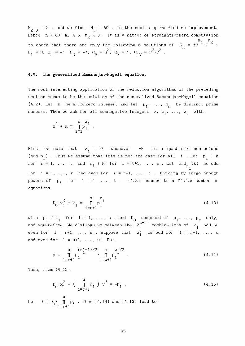
M = 3 , and we find N = 60 . In the next step we find no improvement.2,3 3Hence n < 60, m < 6, m < 3 . It is a matter of straightforward computation

1 2m m1 2

to check that there are only the following 6 solutions of G = +3 W7 :n

2 2 2G = 3, G = -1, G = -7, G = 3 , G = 1, G = 3 W7 .1 2 3 5 7 17

4.9. The generalized Ramanujan-Nagell equation.

The most interesting application of the reduction algorithms of the preceding

section seems to be the solution of the generalized Ramanujan-Nagell equation

(4.2). Let k be a nonzero integer, and let p , ..., p be distinct prime1 s

numbers. Then we ask for all nonnegative integers x, z , ..., z with1 s

s z2 ix + k = p p .

ii=1

First we note that z = 0 whenever -k is a quadratic nonresiduei

(mod p ) . Thus we assume that this is not the case for all i . Let p | ki i

for i = 1, ..., t and p ! k for i = t+1, ..., s . Let ord (k) be oddi p

ifor i = 1, ..., r and even for i = r+1, ..., t . Dividing by large enough

powers of p for i = 1, ..., t , (4.2) reduces to a finite number ofi

equations

s z’2 i

D Wx + k = p p (4.13)0 1 1 i

i=r+1

with p ! k for i = 1, ..., s , and D composed of p , ..., p only,i 1 0 1 r

s-rand squarefree. We distinguish between the 2 combinations of z’ odd or

ieven for i = r+1, ..., s . Suppose that z’ is odd for i = r+1, ..., u

iand even for i = u+1, ..., s . Put

u (z’-1)/2 s z’/2i i

y = p p W p p . (4.14)i i

i=r+1 i=u+1

Then, from (4.13),

u2 ( ) 2

D Wx - p p Wy = -k . (4.15)0 1 9 i 0 1

i=r+1

uPut D = D W p p . Then (4.14) and (4.15) lead to

0 ii=r+1

95

( 2 2v - DWw = k

| 2{ s m , (4.16)

i| v = p p

i9 i=r+1

u uwith v = yW p p , w = x , k = k W p p , and also to

i 1 2 1 ii=r+1 i=r+1

( 2 2v - DWw = k

| 2{ s m , (4.17)

i| w = p p

i9 i=r+1

with v = D Wx , w = y , k = -k WD . We proceed with either (4.16) or0 1 2 1 0

(4.17), which is the most convenient (e.g. the one with the smaller |k | ).2

If D = 1 , then (4.16) and (4.17) are trivial. So assume D > 1 . Let e be

the smallest unit in Z + rDWZ with e > 1 . It is well known that the2 2

solutions v, w of v - DWw = k fall apart into a finite number of2

classes of associated solutions. Let there be T such classes, and choose

for t = 1, ..., T in the t th class the solution v , w such thatt,0 t,0

2 2g = v + w WrD > 1 is minimal. Then all solutions of v - DWw = kt t,0 t,0 2are given by v = +v , w = +w , with

t,n t,n

( n -n )& v = g We + g’We /2

t,n 9 t t 0{ (4.18)

( n -n )7 w = g We - g’We /2WrD

t,n 9 t t 0

8for n e Z , where g’ = v - w WrD . That is, {v } and

t t,0 t,0 t,n n=-88

{w } are linear binary recurrence sequences. Now, (4.16) and (4.17)t,n n=-8

reduce to T equations of type (4.1). If k = 1 , then T = 1, g = e,2 1

-1 2g’ = e . If k | 2WD, k $ 1 , then it is easy to prove that g = |k |We,1 2 2 t 22 -1

g’ = |k |We , so thatt 2

& ( )2n+1 ( )2n+1 *v = r|k |W g /r|k | + g’/r|k | /2 ,t,n 2 7 9 t 2 0 9 t 2 0 8

& ( )2n+1 ( )2n+1 *w = r|k |W g /r|k | - g’/r|k | /2WrD .t,n 2 7 9 t 2 0 9 t 2 0 8

In both cases, (4.16) and (4.17) can be solved by elementary means (see

Section 4.6, of related interest are St3rmer [1897], Mahler [1935], Lehmer

[1964], Rumsey and Posner [1964] and Mignotte [1985]). If k ! 2WD , then we2

s mi

apply the reduction algorithm to one of the equations v = p p ,t,n i

i=r+1

96

s mi

w = p p . Note that n is allowed to be negative, since B = +1 , sot,n i

i=r+1we can use the modified algorithm of Remark 3, Section 4.7.

Thus we have a procedure for solving (4.2) completely. It is well known how

the unit e and the minimal solutions v , w for t = 1, ..., T cant,0 t,0

be computed by the continued fraction algorithm for rD . We conclude this

section with an example. It extends the result of Nagell [1948] (also proved2 z

by many others) on the original Ramanujan-Nagell equation x + 7 = 2 .

2THEOREM_4.14. The only nonnegative integers x such that x + 7 has no

prime divisors larger than 20 are the 16 in the following table.

2 2 | 2x x + 7 1 x x + 7 x x + 7

|----------------------------------------------------------------------------------------------------k------------------------------------------------------------------------------------------------------------------------k-----------------------------------------------------------------------------------------------------------------------------

3 3 20 7 1 7 56 = 2 W7 1 31 968 = 2 W11

3 1 3 1 41 8 = 2 9 88 = 2 W11 35 1232 = 2 W7W11

1 17 8

2 11 1 11 128 = 2 1 53 2816 = 2 W114 1 4 1 9

3 16 = 2 13 176 = 2 W11 75 5632 = 2 W111 1

5 6 155 32 = 2 1 21 448 = 2 W7 1 181 32768 = 2

1 3 3273 74536 = 2 W7W11

1

Proof. Since -7 is a quadratic nonresidue modulo 3, 5, 13, 17 and 19 ,

we have only the primes 2, 7 and 11 left. Only one factor 7 can occur2

in x + 7 , thus we have to solve the two equations

z z2 1 2x + 7 = 2 W11 , (4.19)

z z2 1 2x + 7 = 7W2 W11 . (4.20)

Equation (4.20) can be solved in an elementary way. We distinguish four

cases, each leading to an equation of the type

2 2y - DWz = c

with c | 2WD , and either y or z composed of factors 2 and 11 only.

We have:

z /2 z /21 2

(i) z even, z even, y = 2 W11 , z = x/7, c = 1, D = 7 ;1 2

(z +1)/2 z /21 2

(ii) z odd, z even, y = 2 W11 , z = x/7, c = 2, D = 14 ;1 2

97

z /2 (z -1)/21 2

(iii) z even, z odd, y = x, z = 2 W11 , c = -7, D = 77 ;1 2

(z -1)/2 (z -1)/21 2

(iv) z odd, z odd, y = x, z = 2 W11 , c = -7, D = 154 .1 2

In the first example of Section 4.5 we have worked out case (i). We leave the

other cases to the reader.

Equation (4.19) can be solved by the reduction algorithm. Again we have four

cases, each leading to an equation of the type

2 2y - DWz = c

with z composed of factors 2 and 11 only. We have

z /2 z /21 2

(i) z even, z even, y = x, z = 2 W11 , c = -7, D = 1 ;1 2

(z -1)/2 z /21 2

(ii) z odd, z even, y = x, z = 2 W11 , c = -7, D = 2 ;1 2

z /2 (z -1)/21 2

(iii) z even, z odd, y = x, z = 2 W11 , c = -7, D = 11 ;1 2

(z -1)/2 (z -1)/21 2

(iv) z odd, z odd, y = x, z = 2 W11 , c = -7, D = 22 .1 2

Case (i) is trivial. The other three cases each lead to one equation of type

(4.1). In the example in Section 4.7 we have worked out case (ii). With the

following data the reader should be able to perform Algorithm P by hand for30

the cases (iii) and (iv), thus completing the proof. In these cases N < 10

is a correct upper bound.

Case (iii): a = 10 + 3Wr11 , l = ( 2 + r11 )/2Wr11 ,

y = 0.10011 01000 00110 10100 00110 10110 01001 111101

11011 10010 00001 10110 10111 10100 00110 01101

01010 10010 11101 11001 10000 10010 01010 11011

00010 00111 01110 00101 01101 01111 10101 11110 10.... ,

y = 0.23075 76425 39004 26090 A92A1 03757 07314 58414 7A238.... .2

Case (iv): a = 197 + 42Wr22 , l = ( 9 + 2Wr22 )/2Wr22 ,

y = 0.11101 01101 01110 01010 10111 10001 00100 000111

10000 00110 10101 01100 01101 01111 01101 10101

01011 10100 01100 11101 10011 00011 00010 11110

10101 01100 10011 11111 01001 01110 00000 01110 011.... ,

y = 0.6A001 68184 22921 902A0 724A4 16769 45650 16482 5A6AA.... .2

p

98

Remarks. 1. The computation time for the above proof was less than 2 sec.2 2

2. Let F(X,Y) = aWX + bWXWY + cWY be a quadratic form with integral2

coefficients, and D = b - 4WaWc positive or negative. Let k be a nonzero

integer, and p , ..., p distinct prime numbers. Then we note that1 s

2 24WaWF(X,Y) = (2WaWX+bWY) - DWY ,

so that the diophantine equations

s z s zi i

F(X,k) = p p , F(X, p p ) = ki i

i=1 i=1

in integers X $ 0 and z , ..., z e N , can both be solved by our method.1 s 0

4.10. A mixed quadratic-exponential equation.

In this section we give an application of Algorithm C to the following

diophantine equation. Let

2 2F(X,Y) = aWX + bWXWY + cWY

2be a quadratic form with integral coefficients, such that D = b - 4WaWc is

negative. Let q, v, w be nonzero integers, and p , ..., p distinct prime1 s

numbers. Consider the equation

s mi n

F(X,wW p p ) = vWq (4.21)i

i=1

in integers X , and n, m , ..., m e N .1 s 0

-----Let b, b be the roots of F(x,1) = 0 . Let h be the class number of

Q(rD) . There exists a p e Q(rD) such that we have the principal ideal----- h

equation (p)W(p) = (q ) . Put n = n + hWn , with 0 < n < h . Then1 2 1

nF(X,Y) = vWq is equivalent to finitely many ideal equations

n n----- ----- 2 ----- 2

(aWX-aWbWY)W(aWX-aWbWY) = (s)W(s)W(p) W(p) ,

n----- 1

with (s)Q(s) = (aWvWq ) . Hence we have the equations in algebraic numbers

n n2 ----- 2

& aWX - aWbWY = gWp & aWX - aWbWY = gWp{ n , { n ,

----- ----- ----- 2 ----- ----- 27 aWX - aWbWY = gWp 7 aWX - aWbWY = gWp

99

where g is composed of s , units, and common divisors of aWX - aWbWY and-----

aWX - aWbWY . Note that there are only finitely many choices for g

possible. Thus, (4.21) is equivalent to a finite number of equations

s m n n----- i 2 ----- ----- 2

aW(b-b)WwW p p = gWp - gWp ,i

i=1

n n- 2 ----- ----- 2

or, if we put l = g/aW(b-b) and G = lWp + lWp ,n2

s mi

G = wW p p . (4.22)n i2 i=1

8Here, {G } is a recurrence sequence with negative discriminant. So

n n =02 2

(4.22) is of type (4.1), and can thus be solved by the reduction algorithm of

Section 4.8.

Before giving an example we remark that (4.21) with D > 0 is not solvable

with the methods of this chapter. This is due to the fact that in Q(rD)

with D > 0 there are infinitely many units, hence infinitely many

possibilities for g . Another generalization of equation (4.21) is tot n

n ireplace q by p q . This problem is also not solvable by the method of

ii=1

this chapter, since it does not lead to a binary recurrence sequence if

t > 2 . These problems can however be dealt with by using multi-dimensional

approximation methods, as presented in Chapter 3 and applied in Chapter 7.

We finally present an example.

THEOREM_4.15. The equation

m m m m2 1 2 ( 1 2)2 nX - 3 W7 WX + 2W 3 W7 = 11W2

9 0

in X e Z, n, m , m e N has only the following 24 solutions:1 2 0

n m m X 1 n m m X1 2 1 2

-------------------------------------------------------------------------------------------------------------------------------------------------------------------------------k------------------------------------------------------------------------------------------------------------------------------------------------------1 1 0 -1, 4 1 5 2 0 -10, 19

11 0 0 -4, 5 6 0 0 -26, 27

12 0 0 -6, 7 1 7 0 0 -37, 38

13 0 1 2, 5 7 3 0 2, 25

13 1 0 -7, 10 1 11 1 1 -137, 158

14 0 1 -6, 13 17 2 2 -829, 1270

1

100

Proof. Put b = ( 1 + r-7 )/2 . Then

2 2 -----X - XWY + 2WY = (X-bWY)W(X-bWY) .

Note that Q(r-7) has class number 1 , and that

1 + r-7 1 - r-72 = ----------------------------------- W ----------------------------------- , 11 = ( 2 + r-7 )W( 2 - r-7 ) .

2 2

m m----- ----- 1 2

Suppose g | X - bWY and g | X - bWY . Then g | (b-b)WY = - r-7W3 W7 .n

On the other hand, g | 11W2 . It follows that g = +1 , hence X - bWY and-----

X - bWY are coprime. Thus we have two possibilities:

( 1 + r-7 )nX - bWY = + ( 2 + r-7 )W ----------------------------------- ,

9 2 0

( 1 + r-7 )nX - bWY = + ( 2 - r-7 )W ----------------------------------- ,

9 2 0

in each equation the 2nd and 3rd + being independent. Hence we have to

solve

m m(j) (j) n -----(j) -----n 1 2G = l Wb + l Wb = 3 W7 for j = 1, 2 ,n

(j) (j) (j) (1) -----(2)with G = G - 2WG for j = 1, 2 , and l = l = (2+r-7)/r-7 ,

n+1 n n-1(1) (2) (1) (2) (1) (2)

so that G = G = 1, G = 3, G = -1 . Note that y = -y for0 0 1 1 i i

(1) (2)i = 1, 2 , and j = -j . For j = 1 we have solved (4.22) in the

example of Section 4.8. It is left to the reader to solve (4.22) for j = 2 .

This can be done with the numerical data given for the case j = 1 . p

Remark. The computation time for the above proof was less than 3 sec.

101

dChapter 5. The inequality 0 < x - y < y in S-integers.

The results of this chapter have been published in de Weger [1987].

5.1. Introduction.

Let S be the set of all positive integers composed of primes from a fixed

finite set { p , ..., p } , where s > 2 , and let d e (0,1) . In this1 s

chapter we study the diophantine inequality

d0 < x - y < y (5.1)

in x, y e S . We give explicit upper bounds for the solutions, and we show

how the algorithms for homogeneous, one- and multi-dimensional diophantine

approximation in the real case, that were presented in Chapter 3, can be used

for finding all solutions of (5.1) for any set of parameters p , ..., p ,1 s

d . For s = 2 the continued fraction method (cf. Section 3.2) is used. For3

s > 3 we use the L -algorithm for reducing upper bounds (cf. Section 3.7).

Tijdeman [1973] (see also Shorey and Tijdeman [1986], Theorem 1.1) showed

that there exists a computable number c , depending on max(p ) only, suchi

that for all x, y e S with x > y > 3 ,

cx - y > y/(log y) .

Thus, for any solution of (5.1) a bound for x, y follows. St3rmer [1897]

showed how to solve the equation x - y = k with k = 1, 2 with an

elementary method (see also Mahler [1935], Lehmer [1964]). Our method can

solve this equation for arbitrary k e Z . For the one-dimensional caseb

s = 2 , Ellison [1971 ] has proved the following result: for all but finitelyx y ( )

many explicitly given exceptions, | 2 - 3 | > exp xW(log 2 - 1/10) for9 0

all x, y e N . Cijsouw, Korlaar and Tijdeman (appendix to Stroeker and

Tijdeman [1982]) have found all the solutions x, y e N of the inequality

x y dWx| p - q | < p

1for all primes p, q with p < q < 20 , and with d = ----- . We shall extend

2

102

these results for many more values of p, q and with d = 0.9 . Further, we

determine all the solutions of (5.1) for the multi-dimensional case s = 6 ,1

{ p , ..., p } = { 2, 3, 5, 7, 11, 13 } with d = ----- .1 6 2

In Section 5.2 we derive upper bounds for the solutions of (5.1). In Sections

5.3 and 5.4 we give a method for reducing such upper bounds in the one- and

multi-dimensional cases respectively, and work them out explicitly for some

examples. Section 5.5 contains tables with numerical data.

5.2. Upper bounds for the solutions.

We assume that the primes are ordered as p < ... < p . For a solution1 s

x, y of (5.1), the finitely many z e N for which zWx, zWy is also a

solution of (5.1) can be found without any difficulty. Therefore we may

assume that (x,y) = 1 . Put

X = max ord (xWy) .p

1<i<s i

Put

s9Ws+26 s+4 1 ( )

C = 2 Ws Wmax(1,------------------------------)W p log p Wlog(eWlog p )/(1-d) ,1 log p 9 i0 s-1

1 i=2

C = 2Wlog 2/log p + 2WC Wlog(eWC Wlog p ) .2 1 1 1 s

THEOREM_5.1. The solutions of (5.1) satisfy X < C .2

1 dProof. If y < -----Wx , then y > x - y > y , which contradicts y > 1 . So

21

y > -----Wx . Put L = log(x/y) . Then2

-(1-d) 1 -(1-d)0 < L < x/y - 1 < y < (-----Wx) . (5.2)

2

XBy x = max(x,y) > p , we obtain

1

1-d -(1-d)WX0 < L < 2 Wp . (5.3)

1

We apply Waldschmidt’s result, Lemma 2.4, to L , with n = s, q = 2 . Noten

that the ’independence condition’ [Q(rp ,...,rp ):Q] = 2 holds. Since1 n

p > 3 we have V = log p for i > 2 . Thusi i i

103

( )L > exp -(log X + log(eWlog p ))WC W(1-d)Wlog p .

9 s 1 1 0

Combining this with (5.3) we find

X < C Wlog(eWlog p ) + log 2/log p + C Wlog X .1 s 1 1

2The result now follows from Lemma 2.1, since C > e . p

1

17Examples. With s = 2, 2 < p < 199, d = 0.9 we have C < 2.30*10 ,

i 119

C < 1.97*10 .2

1 33 36With s = 6, 2 < p < 13, d = ----- we find C < 8.37*10 , C < 1.35*10 .

i 2 1 2

5.3. Reducing the upper bounds in the one-dimensional case.

In this section we work out the examples s = 2, d = 0.9 , and p , p run1 2

through either the set of primes below 200, or the set of non-powers below 50

(we did not use that the p are primes). We note that for any other triplei

p , p , d the method works similarly. We prove the following result.1 2

THEOREM_5.2. (a) The diophantine inequality

x x x x d1 2 ( 1 2 )

| p - p | < min p , p (5.4)1 2 9 1 2 0

with p , p primes such that p 2, x > 2, and either d = -----

1 2 1 2 2

x x (5.5)( 1 2 ) 15

or d = 0.9, min p , p > 109 1 2 0

has only the 77 solutions listed in Table I.

(b) The diophantine inequality (5.4) with p , p non-powers such that1 2

2 < p < p < 50 and conditions (5.5), has only the 74 solutions listed in1 2

Table II.

Remarks. The Tables are given in Section 5.5. In Tables I, II the column

"delta" gives the real number with

x x x x delta1 2 ( 1 2 )

| p - p | = min p , p .1 2 9 1 2 0

Note that in Theorem 5.2 we do not demand (x ,x ) = 1 , and in Theorem1 2

104

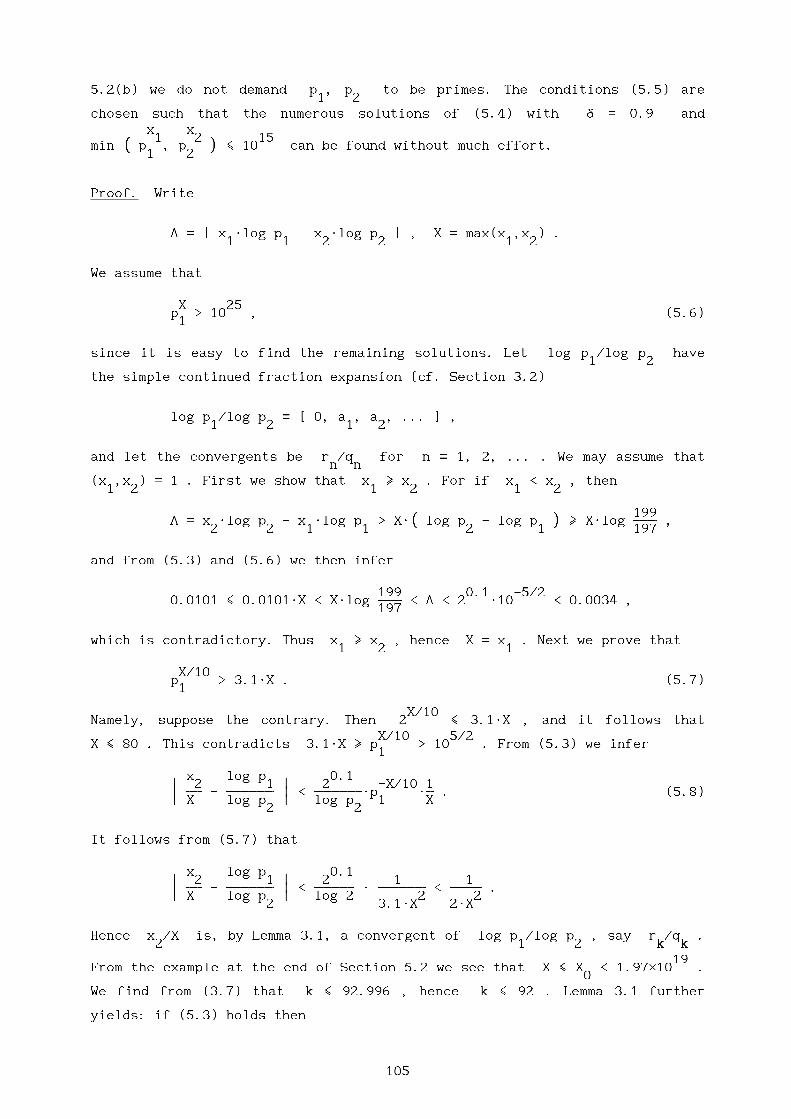
5.2(b) we do not demand p , p to be primes. The conditions (5.5) are1 2

chosen such that the numerous solutions of (5.4) with d = 0.9 andx x

( 1 2 ) 15min p , p < 10 can be found without much effort.

9 1 2 0

Proof. Write

L = | x Wlog p - x Wlog p | , X = max(x ,x ) .1 1 2 2 1 2

We assume that

X 25p > 10 , (5.6)1

since it is easy to find the remaining solutions. Let log p /log p have1 2

the simple continued fraction expansion (cf. Section 3.2)

log p /log p = [ 0, a , a , ... ] ,1 2 1 2

and let the convergents be r /q for n = 1, 2, ... . We may assume thatn n

(x ,x ) = 1 . First we show that x > x . For if x < x , then1 2 1 2 1 2

( ) 199L = x Wlog p - x Wlog p > XW log p - log p > XWlog --------------- ,

2 2 1 1 9 2 1 0 197

and from (5.3) and (5.6) we then infer

199 0.1 -5/20.0101 < 0.0101WX < XWlog --------------- < L < 2 W10 < 0.0034 ,

197

which is contradictory. Thus x > x , hence X = x . Next we prove that1 2 1

X/10p > 3.1WX . (5.7)1

X/10Namely, suppose the contrary. Then 2 < 3.1WX , and it follows that

X/10 5/2X < 80 . This contradicts 3.1WX > p > 10 . From (5.3) we infer

1

x log p 0.1| 2 1 | 2 -X/10 1| ---------- - ------------------------------ | < ------------------------------Wp W----- . (5.8)| X log p | log p 1 X

2 2

It follows from (5.7) that

x log p 0.1| 2 1 | 2 1 1| ---------- - ------------------------------ | < ------------------------- W ------------------------------ < -------------------- .| X log p | log 2 2 2

2 3.1WX 2WX

Hence x /X is, by Lemma 3.1, a convergent of log p /log p , say r /q .2 1 2 k k

19From the example at the end of Section 5.2 we see that X < X < 1.97*10 .

0We find from (3.7) that k < 92.996 , hence k < 92 . Lemma 3.1 further

yields: if (5.3) holds then

105

q /10 log pk 1 2

a > -2 + p W----------W------------------------------ , (5.9)k+1 1 q 0.1

k 2

and if

q /10 log pk 1 2

a > p W----------W------------------------------ (5.10)k+1 1 q 0.1

k 2

then (5.3) holds for (x ,x ) = (q ,r ) . We computed the continued fraction1 2 k k

expansions and the convergents of all numbers log p /log p in the1 2

mentioned ranges for p , p exactly up to the index n such that1 2

19q < 1.97*10 < q (cf. Section 2.5 for details of the computationaln-1 nmethod). Note that n < 93 . We checked all convergents for (5.9), and

subsequently for (5.10). It is possible, though unlikely, that there is a

convergent that satisfies (5.9) but fails (5.10). We met only one such a

case: p = 15, p = 23 , with log 15/log 23 = [ 0, 1, 6, 2, 1, 51, ...] ,1 2

so that a = 51, r = 19, q = 22 . Now, (5.9) holds but (5.10) fails, since5 4 4

2.2 1 0.115 W----------W(log 19)/2 = 51.4... e [51,53) .

22

0.1 -2.2We have in this case L = 0.002714... < 0.002771... = 2 W15 , so (5.3)

22 19 19is true. But log(15 -23 )/log(23 ) = 0.9008... > d , so (5.1) is not

true. This example illustrates that (5.3) is weaker than (5.1). Therefore all

found solutions of (5.3) have been checked for (5.1) as well. The proof is

now completed by the details of the computations, which we omit here. p

Remarks. 1. Theorem 5.2(a) is used in the proof of Theorem 6.2.

2. The computations for the proof of Theorem 5.2 took 35 sec.

5.4. Reducing the upper bounds in the multi-dimensional case.

Now let s > 3 . Put x = ord (x/y) for i = 1, ..., s . Theni p

iX = max|x | , and

i

sL = S x Wlog p .

i ii=1

Note that (5.3) is of the form (3.1). Hence by Theorem 5.1 we can use the

method described in Section 3.7 for solving (5.3). We shall do so for the

example s = 6, { p , ..., p } = { 2, 3, 5, 7, 11, 13 } (the first six1 6

1primes), and d = ----- .

2

106

We use small refinements of Lemmas 3.7 and 3.8, devised specially for this

application, as follows. Let notation be as in Section 3.7.

LEMMA_5.3. Let X be a positive number such that1

( 2 2)l(G) > r 4Wn +(n-1)Wg WX . (5.11)

9 0 1

Then (5.3) has no solutions with for i = 1, ..., s

( ) 1log gWCWr2/sWX /-----Wlog p < |x | < X < X . (5.12)

9 10 2 i i 1

LEMMA_5.4. Suppose that

s~|L| > S |x | . (5.13)

ii=1

Then

s& ( )*

|x | < log gWCWr2/ |l|- S |x | /(1-d)Wlog p . (5.14)i 7 9 i 08 i

i=1

Remark. Lemmas 5.3 and 5.4 are refinements of Lemma 3.8, in that they

differentiate between the different x . Moreover, Lemma 5.3 has slightlyi

sharper condition and conclusion than Lemma 3.7.

Proofs_(of_Lemmas_5.3_and_5.4). Analogous to the proofs of Lemmas 3.7 and

3.8, using (5.2) and

|x |i -1/2

p < max(x,y) = x < 2W|L| . pi

THEOREM_5.5. The diophantine inequality

0 < x - y < ry

x x1 6

in x, y e S = { 2 W...W13 | x e N for i = 1, ..., 6 } withi 0

(x,y) = 1 has exactly 605 solutions. Among those, 571 satisfy

ord (xWy) < 19 , ord (xWy) < 12 , ord (xWy) < 8 ,2 3 5

ord (xWy) < 7 , ord (xWy) < 5 , ord (xWy) < 5 .7 11 13

The remaining 34 solutions are listed in Table III.

107

Remark. The upper bounds for ord (xWy) given for the 571 solutions notpi

listed in Table III are chosen such that it takes a reasonable amount of

computer time to find them all by a brute force method. The list of all 605

solutions is too extensive to be reproduced here.

Proof. By the example at the end of Section 5.2 we know that X < X for0

36X = 1.35*10 . We apply the method described in Section 3.7. Take0

240 6C = 10 (which is chosen so that it is somewhat larger than X ), and

03

g = 1 . We applied the L -algorithm to the corresponding lattice G , and1

39found a reduced basis c , ..., c with |c | > 9.40*10 . By Lemma 3.4,

1 6 1

-5/2 39 39l(G ) > 2 W9.40*10 > 1.66*10 .

1

( 2 2) 37This is larger than r 4W6 +5W1 WX = 1.64...*10 , so (5.11) holds with

9 0 0X = X . By Lemma 5.3 we find1 0

( 240 36) 1X < log 10 Wr2/6W1.35*10 /-----Wlog 2 < 1350.4 ,

9 0 2

32so X < 1350 . Next we choose C = 10 , g = 1 , and X = 1350 . The reduced

0basis of the corresponding lattice G was computed, and we found

25 4

|c | > 2.71*10 . Hence l(G ) > 4.79*10 , which is larger than1 2

4r149W1350 = 1.64...*10 . Hence Lemma 5.3 yields for all i = 1, ..., 6

( 32 ) 1|x | < log 10 Wr2/6W1350 /-----Wlog p ,i 9 0 2 i

and it follows that

|x | < 187 , |x | < 118 , |x | < 80 ,1 2 3

(5.15)

|x | < 66 , |x | < 54 , |x | < 50 .4 5 6

12 4Next we choose C = 10 , g = 10 . We use Lemma 5.4 as follows. If

6|l| > 10 then (5.13) holds by (5.15), and Lemma 5.4 yields

|x | < 67 , |x | < 42 , |x | < 29 ,1 2 3

(5.16)

|x | < 24 , |x | < 19 , |x | < 18 .4 5 6

All vectors in the corresponding lattice G satisfying (5.15) and3

6|l| < 10 have been computed with the Fincke and Pohst algorithm, cf.

Section 3.6. We omit details. We found that there exist only two such

vectors, but they do not correspond to solutions of (5.1). Hence all8 4

solutions of (5.1) satisfy (5.16). Next, we choose C = 10 , g = 10 . If

108

5|l| > 5*10 then Lemma 5.4 yields

|x | < 42 , |x | < 27 , |x | < 18 ,1 2 3

(5.17)

|x | < 15 , |x | < 12 , |x | < 11 .4 5 6

There are 143 vectors in the corresponding lattice G satisfying (5.16)4

5and |l| < 5*10 . Of them, 2 correspond to solutions of (4.1), namely those

with

(x ,...,x ) = ( 7, -5, 3, -9, -3, 8) , l = 257674 ,1 6

(x ,...,x ) = (-10, 10, -6, 5, -6, 4) , l = 144817 .1 6

Both also satisfy (5.17). Hence all solutions of (5.1) satisfy (5.17). At

this point it seems inefficient to choose appropriate parameters C, g , and

a bound for |l| to repeat the procedure with. But the bounds of (5.17) are

small enough to admit enumeration. Doing so, we found the result. p

Remark. Theorems 5.2 and 5.5 find applications in solving other exponentiala

diophantine equations, see Stroeker and Tijdeman [1982], Alex [1985 ],b

[1985 ], Tijdeman and Wang [1988], and Section 6.4 of this book.

Remark. The computation of the reduced basis of G took 113 sec, where we1

3applied the L -algorithm as we described it in Section 3.5, in 12 steps. The

direct search for the solutions of (5.17) took 228 sec. The remaining

computations (computation of the log p up to 250 decimal digits, of thei

reduced basis of G , and of the short vectors in G and G ) took 8 sec.2 3 4

Hence in total we used 349 sec.

109

5.5. Tables.

Table_I. (Theorem 5.2(a)).

(overdwars over blz. 110-111, de tabel van het proefschrift blz. 114-115)

110

bdeweger

Rectangle

bdeweger

Stamp

bdeweger

Rectangle

111

bdeweger

Stamp

Table_II. (Theorem 5.2(b)).

(overdwars over blz. 112-113, de tabel van het proefschrift blz. 116-117)

112

bdeweger

Stamp

bdeweger

Rectangle

113

bdeweger

Stamp

Table_III_. (Theorem 5.5).

(de tabel van het proefschrift blz. 113)

114

bdeweger

Stamp

Chapter 6. The equation x + y = z in S-integers.

The results of this chapter have been published in de Weger [1987].

6.1. Introduction.

Let S be the set of all positive integers composed of primes from a fixed

finite set { p , ..., p } , where s > 3 . This chapter is devoted to the1 s

diophantine equation

x + y = z (6.1)

in x, y, z e S . Without loss of generality we may assume that x, y, z are

relatively prime. For any a e S we define

m(a) = max ord (a) .p

1<i<s i

It was proved by Mahler [1933] that (6.1) has only finitely many solutions,

but his proof is ineffective. An effective version, i.e. an effectively

computable upper bound for m(xWyWz) for the solutions x, y, z of (6.1),v

can be derived from the results of Coates [1969], [1970] and Sprindzuk

[1969], since (6.1) can be reduced to a finite number of Thue equations. See

also Chapter 1 of Shorey and Tijdeman [1986].

We derive an explicit upper bound in Section 6.2. Section 6.3 is devoted to

some details of the p-adic approximation lattices on which the reduction

method of Sections 6.4 and 6.5 are based. In Section 6.4 we give a method of

solving (6.1) in the one-dimensional case s = 3 . This method is based on

the reduction procedure given in Section 3.10, and we also use a combination

of p-adic and real approximation techniques, similar to that of Section 4.8.

But instead of actually performing the real reduction step, we now can simply

refer to the results of Chapter 5. As an example we find all the solutions of

the slightly more general equation x + y = wWz , where x, y, z are powers

of 2, 3 or 5 , and w e Z , |w| < 1000000 , (w,z) = 1 .

115

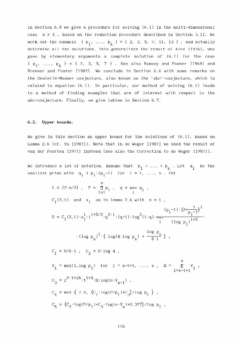
In Section 6.5 we give a procedure for solving (6.1) in the multi-dimensional

case s > 4 , based on the reduction procedure described in Section 3.11. We

work out the example { p , ..., p } = { 2, 3, 5, 7, 11, 13 } , and actually1 6

determine all the solutions. This generalizes the result of Alex [1976], who

gave by elementary arguments a complete solution of (6.1) for the case

{ p , ..., p } = { 2, 3, 5, 7 } . See also Rumsey and Posner [1964] and1 4

Brenner and Foster [1982]. We conclude in Section 6.6 with some remarks on

the Oesterlw-Masser conjecture, also known as the ’abc’-conjecture, which is

related to equation (6.1). In particular, our method of solving (6.1) leads

to a method of finding examples that are of interest with respect to the

abc-conjecture. Finally, we give tables in Section 6.7.

6.2. Upper bounds.

We give in this section an upper bound for the solutions of (6.1), based on

Lemma 2.6 (cf. Yu [1987]). Note that in de Weger [1987] we used the result of

van der Poorten [1977] instead (see also the Correction to de Weger [1987]).

We introduce a lot of notation. Assume that p < ... < p . Let q be the1 s i

smallest prime with q ! p W(p -1) for i = 1, ..., s . Puti i i

st = [2Ws/3] , P = p p , q = max q ,

i ii=1 i

C (2,t) and a as in lemma 2.6 with n = t ,1 1

( 1 )t(p -1)W 2+--------------------i 9 p -10

t t+5/2 2Wt 2 iU = C (2,t)Wa Wt Wq W(q-1)Wlog (tWq)Wmax--------------------------------------------------------------------------------W

1 1 t+2i (log p )

i

log pt ( s )

W(log p ) W log(4Wlog p ) + ------------------------------ ,s 9 s 8Wt 0

C = U/6Wt , C = UWlog 4 ,1 2

sV = max(1,log p ) for i = s-t+1, ..., s , W = p V ,i i i

i=s-t+1

9Wt+26 t+4C = 2 Wt WWWlog(eWV ) ,3 s-1

( ( ) )C = max 7.4, C Wlog(P/p )+C /log p ,4 9 9 1 1 30 1 0

( )C = C Wlog(P/p )+C Wlog(eWV )+0.327 /log p ,5 9 2 1 3 s 0 1

116

( )C = max C , (C Wlog(P/p )+log 2)/log p ,6 9 5 2 1 1 0

( )C = 2W C + C Wlog C ,7 9 6 4 4 0

p( ( s) )

C = max p , log 2W(P/p ) /log p , C +C Wlog C , C .8 9 s 9 1 0 1 2 1 7 7 0

Now we state the main result.

THEOREM_6.1. The solutions of (6.1) satisfy m(xWyWz) < C .8

Proof. If we consider instead of (6.1) the equivalent equation

x + y = z (6.2)

then we may assume that xWy has at most t prime divisors, p , ..., pi i1 t

say. Suppose first that m(xWy) p and m(z) > 2 . Then for some p = p ,s i

x xm(z) = ord (z) = ord [ +----- - 1 ] = ord [log (-----)] .

p p y p p y

xt i

jPut x/y = p p . Then m(xWy) = max |x | . We apply Lemma 2.6 (Yu’s

i ij=1 j 1<j<t j

lemma) with n = t, B = B = B’ = B = m(xWy) . Since m(xWy) > p and0 n s

t > 2 we have

3W = max [ log(1+---------------WB), log B, log p ] = log B .

4Wt

Note that C (p,n) is maximal for p = 2 . We obtain1

m(z) < C Wlog m(xWy) + C . (6.3)1 2

Obviously (6.3) is true if m(z) < 2 . If in (6.2) the plus sign holds, then

m(z) m(xWy)(P/p ) > z > max(x,y) > p .

1 1

By (6.3) and C > 0 it then follows that3

117

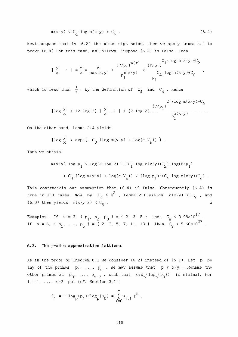
m(xWy) < C Wlog m(xWy) + C . (6.4)4 6

Next suppose that in (6.2) the minus sign holds. Then we apply Lemma 2.4 to

prove (6.4) for this case, as follows. Suppose (6.4) is false. Then

C Wlog m(xWy)+Cm(z) 1 2

(P/p ) (P/p )y z z 1 1

| ----- - 1 | = ----- = ---------------------------------------- < -------------------------------------------------- < -------------------------------------------------------------------------------------------------------------- ,x x max(x,y) m(xWy) C Wlog m(xWy)+C

p 4 61 p

1

1which is less than ----- , by the definition of C and C . Hence

2 4 6

C Wlog m(xWy)+C1 2

(P/p )y y 1

|log -----| < (2Wlog 2)W| ----- - 1 | < (2Wlog 2)W-------------------------------------------------------------------------------------------------------------- .x x m(xWy)

p1

On the other hand, Lemma 2.4 yields

y ( )|log -----| > exp -C W(log m(xWy) + log(eWV )) .

x 9 3 s 0

Thus we obtain

m(xWy)Wlog p < log(2Wlog 2) + (C Wlog m(xWy)+C )Wlog(P/p )1 1 2 1

+ C W(log m(xWy) + log(eWV )) < (log p )W(C Wlog m(xWy)+C ) .3 s 1 4 6

This contradicts our assumption that (6.4) if false. Consequently (6.4) is2

true in all cases. Now, by C > e , Lemma 2.1 yields m(xWy) < C , and4 7

(6.3) then yields m(xWyWz) < C . p8

17Examples. If s = 3, { p , p , p } = { 2, 3, 5 } then C < 3.98*10 .

1 2 3 827

If s = 6, { p , ..., p } = { 2, 3, 5, 7, 11, 13 } then C < 5.60*10 .1 6 8

6.3. The p-adic approximation lattices.

As in the proof of Theorem 6.1 we consider (6.2) instead of (6.1). Let p be

any of the primes p , ..., p . We may assume that p ! xWy . Rename the1 s

other primes as p , ..., p , such that ord (log (p )) is minimal. For0 s-2 p p 0

i = 1, ..., s-2 put (cf. Section 3.11)

8l

y = - log (p )/log (p ) = S u Wp ,i p i p 0 i,l

l=0

118

where u e { 0, 1, ..., p-1 } . The y take the place of the y’ ofi,l i i

Section 3.11. Then it is clear from Section 3.11 how to define the p-adic

approximation lattices G for m e N . Putm 0

s-2L = S x Wy - x .

i i 0i=1

Then Lemma 3.13 yields

-mG = { (x ,...,x ,x ) | |L| < p }m 1 s-2 0 p

s-2 x -(m+m )| & i*| 0

= { (x ,...,x ,x ) | |log p p | < p } ,1 s-2 0 | p7 i 8|p

i=0

where m = ord (log (p )) . In Section 3.13 we studied the set0 p p 0

s-2 x -(m+m )* | i | 0G = { (x ,...,x ,x ) | | p p + 1| 5 it happens to be possible to choose p such that not only0

ord (log (p )) is minimal, but also p is a primitive root (mod p) .p p 0 0

Then, using the notation of Lemma 3.17 (with b as the last element of the0

basis), choose z _ p (mod p) . Then k(b ) = 1 , and it follows that0 0

( (m))Tb’ = b for i = 1, ..., s-2 . By b = 0,...,1,...,0,y we havei i i 9 i 0

(m)y k(b ) m+mi i 0

p Wp _ z (mod p ) .i 0

ai

If p _ p (mod p) , then it follows thati 0

m-1* (m)g _ a + y _ a + S u (mod (p-1)/2) for i = 1, .., s-2 ,i i i i i,l

l=0

*g = (p-1)/2 .0

Lemma 3.14 (with c = 0, c = 1 ) now yields: if1 2

*l(G ) > r(s-1)WX (6.5)

m 1

then (6.2) has no solutions with

m + m < ord (z) < m(xWyWz) < X . (6.6)0 p 1

119

6.4. Reducing the upper bounds in the one-dimensional case.

In Section 3.10 we have described how an upper bound for the solutions of

(6.1) in the case s = 3 can be reduced. We shall apply that method in this

section to the following problem.

THEOREM_6.2. The diophantine equation

x + y = wWz , (6.7)

x x0 1 u

where x = p , y = p , z = p , (p,p ,p ) = (2,3,5), (3,2,5), (5,2,3) ,0 1 0 1

6x , x , u e N , w e Z, |w| < 10 , and p ! w , has exactly 291 solutions0 1 0for p = 2 , 412 solutions for p = 3 , and 570 solutions for p = 5 . In

Table I all solutions with u > 3 are given. The solutions with u < 2

satisfy x < 14, x < 9 for p = 2 , x < 23, x < 10 for p = 3 , and0 1 0 1

x < 25, x < 15 for p = 5 .0 1

Remark. It is easy to find all solutions of (6.7) with u < 2 . The Tables

are presented in Section 6.7.

Proof. Put X = max ord (xWyWz) . The example at the end of Section 6.2p

p=2,3,517

shows that in the case |w| = 1 we have X < 3.98*10 . It can be checked6

without difficulties that the effect of the w with |w| < 10 in the proof

of Theorem 6.1 can be neclected (it disappears in the rounding off), so that17

for the solutions of (6.7) also X < X = 3.98*10 holds. Put0

y y0 1

x/y = p Wp , y = - log (p )/log (p ) .0 1 p 1 p 0

*Note that y is a p-adic integer. Define the lattices G , G as in Section

m m

6.3, so G is generated bym

& 1 * & 0 *b = | | , b = | | .1 (m) 0 m

7 y 8 7 p 8

* *For p = 2, 3 we have G = G , and for p = 5 a basis of G is

m m m

* *b = b - gWb , b = 2Wb ,1 1 0 0 0

(m) (m)where g = 0 if y is odd, g = 1 if y is even . Using the

algorithm given in Section 3.10, Fig. 3, we can compute a basis c , c of1 2

* *G that is reduced in the sense that |c | = l(G ) . We did so, with m asm 1 m

120

in the following table.

1p p p m m g |c | > u < W |y | < |y | <

0 1 1 0 1 0 1-----------------------------------------------------------------k---------------------------------------------------------------------------------------------------------------------------------------------------------------------------------------------------------------------------------------------------------------------------------------------

21 6 1442 3 5 1 2 143 - 2.68*10 144 10 W2 114 78

1 21 6 913 2 5 1 91 - 2.32*10 91 10 W3 182 78

122 6 65

5 2 3 1 1 65 0 5.28*10 65 10 W5 189 119

(m)The values of y can be found in Table III. Making an exception to our

*policy, we give the reduced bases of the G below (in base p notation):

m

( )p = 2 : 10 00000 00100 10001 10110 01110 01101

| || 00001 11101 00101 00100 11100 01111 11010 00011 |

c = | | ,1

| - 1 00010 00110 01000 01011 01110 00010 || |00101 11000 00000 11100 01111 01011 10111 00001

9 0

( )10 11011 10000 01011 01101 11000 00111

| || 11001 10100 11011 00000 11111 10110 10110 00001 |

c = | | ,2

| 10 01110 11101 10111 11000 00100 10101 || |00111 00001 10101 00110 10011 00111 00101 10101

9 0

p = 3 : & - 102 01121 02221 00210 12120 20020 22222 10212 20222 *c = | | ,1

7 21002 00122 21100 11102 22102 20001 11222 02212 21011 8

& -10 12210 12111 01102 02010 12112 12210 21122 21011 20102 *c = | | ,2

7 - 2 22021 11012 01000 12021 00211 12221 22121 21220 12122 8

p = 5 : & - 211 32230 21042 22023 30141 33034 21420 *c = | | ,1

7 - 22104 43102 43111 03114 30134 23410 8

& 340 34003 02404 12120 03412 22030 32211 *c = | | .2

7 - 414 20001 42202 42210 34043 20120 00432 8

From this we found the lower bounds for |c | given above. They are all1

17larger than r2W3.98*10 . Hence (6.5) holds for X = X , and then we

1 0infer from (6.6) that u < m + m - 1 , and |w|Wz < W as shown in the table

0above. We now find the new upper bounds for |y |, |y | as follows. If in

0 110/9

(6.7) the minus sign holds, supposing that min(x,y) > W , we infer

0.9| x - y | = |w|Wz < W < min(x,y) .

121

0.9By Theorem 5.2(a), the inequality | x - y | < min(x,y) has no solutions

49 10/9with min(x,y) > W , since W > 10 . Hence min(x,y) < W , and thus

10/9max(x,y) < min(x,y) + |w|Wz < W + W .

If in (6.7) the plussign holds, then this inequality follows at once. So now

the bounds given in the above table for |y |, |y | follow from0 1

10/9|y |Wlog p < log max(x,y) < log(W +W) .i i

We repeat the procedure with m as in the following table.

1p m g |c | > r2WX < u < W |y | < |y | <

1 1 0 0 1--------------------k-----------------------------------------------------------------------------------------------------------------------------------------------------------------------------------------------------------------------------------------------------------------------------------------------------------------------------------------------

6 172 1 16 - 167.7 161.3 17 10 W2 31 21

1 6 133 13 - 535.8 257.4 13 10 W3 49 21

16 7

5 1 7 1 276.1 267.3 7 10 W5 49 31

The numbers are now so small that the computations can be performed by hand.*

For example, for p = 5 , the lattice G is generated by7

& 1 * & 0 ** *b = | | , b = | | ,1 0

7 -45607 8 7 156250 8

and a reduced basis is

& 185 * & -394 *c = | | , c = | | .1 0

7 205 8 7 408 8

We find upper bounds for u and W as given in the above table. In all10/9 15 15

three cases, W < 10 . On supposing min(x,y) > 10 we infer

15W0.9 0.9| x - y | = |w|Wz < W < 10 < min(x,y) .

0.9By Theorem 5.2(a) we see that the inequality | x - y | < min(x,y) has

65 28 84 53only two solutions: (x,y) = (2 ,5 ), (2 ,3 ) . However, both have

15W0.9 15| x - y | > 10 . So we infer min(x,y) < 10 , hence by

15max(x,y) < 10 + W we obtain the bounds for |y |, |y | as given above.

0 1These bounds are small enough to admit enumeration of the remaining cases. p

Remark. The computer calculations for the above proof took less than 1 sec.

122

6.5. Reducing the upper bounds in the multi-dimensional case.

In Section 3.11 we have described how an upper bound for the solutions of

(6.1) in the case s > 3 can be reduced. We shall apply that method in this

section to the following problem.

THEOREM_6.3. The diophantine equation

x + y = z (6.8)

x x1 6

in x, y, z e S = { 2 W...W13 | x e N for i = 1, ..., 6 } withi 0

(x,y) = 1 and x < y has exactly 545 solutions. Of them, 514 satisfy

ord (xWyWz) < 12 , ord (xWyWz) < 7 , ord (xWyWz) < 5 ,2 3 5

ord (xWyWz) < 4 , ord (xWyWz) < 3 , ord (xWyWz) < 3 .7 11 13

The remaining 31 solutions are given in Table II.

Remark. From Theorem 6.3 it is easy to compute all 545 solutions of (6.8).

Proof. In the example at the end of Section 6.2 we have seen that27

m(xWyWz) < X = 5.60*10 . With the notation of Section 6.3 we choose the0

following parameters.

1 * * * * *p p p p p p m m g g g g g

1 0 1 2 3 4 0 0 1 2 3 4---------------k-------------------------------------------------------------------------------------------------------------------------------------------------------------------------------------------------------------------------------------------------------------------------------------------------------2 1 3 5 7 11 13 2 605 - - - - -

13 2 5 7 11 13 1 385 - - - - -

15 1 2 3 7 11 13 1 275 2 0 1 1 1

17 3 2 5 11 13 1 220 3 0 -1 -1 0

111 1 2 3 5 7 13 1 165 5 2 0 -1 -1

113 2 3 5 7 11 1 165 6 -2 -1 -2 3

1

(m)We computed the six values of the y for i = 1, 2, 3, 4 (and give them

i*

in Table III), and the reduced bases of the six lattices G , by them

3 *L -algorithm. Thus we obtained lower bounds for l(G ) as in the following

m27

table. They are all larger than r5W5.60*10 (note that we have a very

large margin here, we could have taken the m’s probably about 20% smaller).27

So we apply Lemma 3.14 for X = X = 5.60*10 . For every p we thus find1 0

ord (z) < m + m - 1 . Since (6.2) is invariant under permutations of x, y,p 0

z , we even have ord (xWyWz) < m + m - 1 , as shown in the next table.p 0

123

1 *p l(G ) > |c |/4 > ord (xWyWz) <

1 m 1 p------------------------------k---------------------------------------------------------------------------------------------------------------------------------------------------------------------------------------------

352 1 4.70*10 606

1 363 1.15*10 385

137

5 1 6.27*10 2751 36

7 3.17*10 2201

3311 1 5.74*10 165

1 3613 1.73*10 165

1

Hence m(xWyWz) < 606 .

We repeated the procedure with X = 606 and m as in the following table.0

*After computing the reduced bases of the six lattices G we found the

m*

following data. Note that in all cases l(G ) > r5W606 .m

1 * * * * * *p m g g g g g l(G ) > ord (xWyWz) <

1 0 1 2 3 4 m p---------------k---------------------------------------------------------------------------------------------------------------------------------------------------------------------------------------------------------------------------------------------------------------------------------------2 1 66 - - - - - 1909 67

13 42 - - - - - 2304 42

15 1 30 2 0 0 1 1 3417 30

17 24 3 -1 0 1 -1 2391 24

111 1 18 5 0 -2 2 -1 1443 18

113 18 6 0 1 1 -2 3196 18

1

Hence m(xWyWz) < 67 . Next, we repeated the procedure with X = 67 , and m0

as in the following table. We found

1 * * * * * *p m g g g g g l(G ) > ord (xWyWz) <

1 0 1 2 3 4 m p---------------k---------------------------------------------------------------------------------------------------------------------------------------------------------------------------------------------------------------------------------------------------------------------------------------2 1 55 - - - - - 364 56

13 35 - - - - - 301 35

15 1 25 2 1 1 1 0 622 25

17 20 3 -1 1 -1 0 693 20

111 1 15 5 -1 -2 2 2 192 15

113 15 6 -1 0 3 -2 658 15

1

Hence m(xWyWz) < 56 .

To find the solutions of (6.2) with ord (xWyWz) below the bounds given inp

the above table, we followed the following procedure. Suppose that we are at

a certain moment interested in finding the solutions with ord (xWyWz) < f(p)p

where f(p) is given for p = 2, ..., 13 . Choose p , and m < f(p) - m ,0

124

*and consider the lattice G for these values of p, m . If a solution

m

x, y, z of (6.2) exists with ord (z) > m + m , then the vectorp 0

( )Tx ,...,x ,x with x = ord (x/y) for i = 0, ..., 4 , is in the9 1 4 00 i p

i( 2 2) *

lattice. Its length is bounded by r f(p ) +...+f(p ) . All vectors in G9 0 4 0 m

with length below this bound can be computed by the algorithm of Fincke and

Pohst, as given in Section 3.6. Then all solutions of (6.2) corresponding to

lattice points can be selected. Then we replace f(p) by m + m - 1 , and0

we repeat the procedure for newly chosen p, m .

We performed this procedure, starting with the bounds for ord (xWyWz) givenp

in the above table for f(p) , and with p, m as in Table IV (where #

stands for the number of solutions of (5.2) found at that stage). At the end

we have f(2) = 4 , f(p) = 1 for p = 3, ..., 13 . The remaining solutions

can be found by hand. p

Remarks. 1. Theorems 6.2 and 6.3 have applications in group theory (cf. Alex

[1976]). We use Theorem 6.3 in Section 7.2.

2. The computer calculations for the proof of Theorem 6.3 took 438 sec., of

which 412 were used for the first reduction step. In this first step we3

applied the L -algorithm in 11 steps (cf. Section 3.5), which cost on average

about 60 sec. per lattice. The remaining 50 sec. were mainly used for the(m)

computation of the 24 y ’s .i

6.6. Examples related to the abc-conjecture.

Let x, y, z be positive integers. Put

G = p p .p|xyzp prime

For all x, y, z with (x,y) = 1 and x + y = z we define

c(x,y,z) = log z / log G

(called the Masser-ratio, according to Tijdeman [1989]). Recently, Oesterlw

posed the problem to decide whether there exists an absolute constant C

such that c(x,y,z) < C for all x, y, z . Masser [1985] conjectured the

stronger assertion that c(x,y,z) < 1 + e , when z exceeds some bound

depending on e only, for all e > 0 . For a survey of related results and

conjectures, see Stewart and Tijdeman [1986], Vojta [1987], Tijdeman [1989].

125

It might be interesting to have some empirical results on c(x,y,z) , and to

search for x, y, z for which it is large. From the preceding sections it

may be clear that such x, y, z correspond to relatively short vectors in

appropriate p-adic approximation lattices.

As a byproduct of the proofs of Theorems 5.5 and 6.3 we computed the value of

c(x,y,z) , corresponding to many short vectors that we came across in

performing the algorithm of Fincke and Pohst. All examples that we found with

c(x,y,z) > 1.4 are listed below. Our search was rather unsystematic, so we

do not guarantee that this list is complete in any sense.

x y z c(x,y,z)-------------------------------------------------------------------------------------------------------------------------------------------------------------------------------------------------------------------------------------------------------------------------------------------------------

2 2 6 3 2111 3 W5 W7 2 W23 1.62599

7 41 2W3 5 W7 1.567893 10 117 3 2 W29 1.547082 13 18 7 25 W7937 7 2 W3 W13 1.497622 9 11 3

11 3 W13 2 W5 1.4888715 8

37 2 3 W5 1.482917 2 6 62 W5 7 W41 13 1.46192

5 2 41 2 W3W5 7 1.4556719 11 11 3 22 W13W103 7 3 W5 W11 1.45261

12 3 5 21 2 W5 3 W7 W43 1.44331

4 7 8 21 2 W3 W547 5 W7 1.4390610 7 82 W7 5 3 W13 1.43501

3 73 5 2 1.42657

11 105 3 2 W173 1.41268

Two more examples with c(x,y,z) > 1.4 are known:

2 18x = 1 , y = 3W5W47 , z = 2 W79 , c(x,y,z) = 1.44965 ,

found by G. Frey (communicated to us by Prof. F. Oort), and

10 5x = 2 , y = 109W3 , z = 23 , c(x,y,z) = 1.62991 ,

found by E. Reyssat (communicated to us by Prof. M. Waldschmidt), which wins

the race. Note that these two examples show large primes at two places.

These results do not seem to yield any heuristical evidence for the truth or

falsity of the abc-conjecture.

126

6.7. Tables.

Table_I. (Theorem 6.2.)


127

bdeweger

Stamp

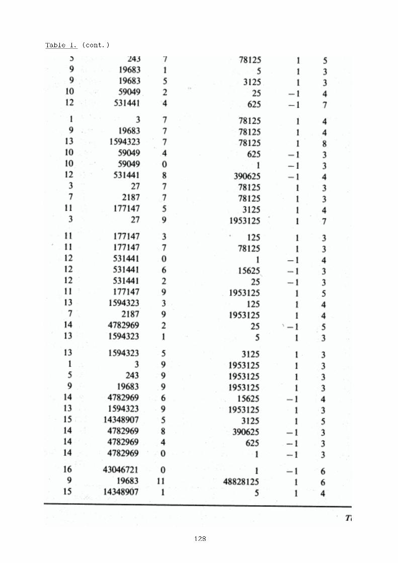
Table_I. (cont.)


128

bdeweger

Stamp

Table_I. (cont.)


129

bdeweger

Stamp

Table_II. (Theorem 6.3.)


130

bdeweger

Rectangle

bdeweger

Stamp

Table_III.


131

bdeweger

Stamp

Table_III. (cont.)


132

bdeweger

Stamp

Table_III. (cont.)


133

bdeweger

Stamp

Table_III. (cont.)


134

bdeweger

Stamp

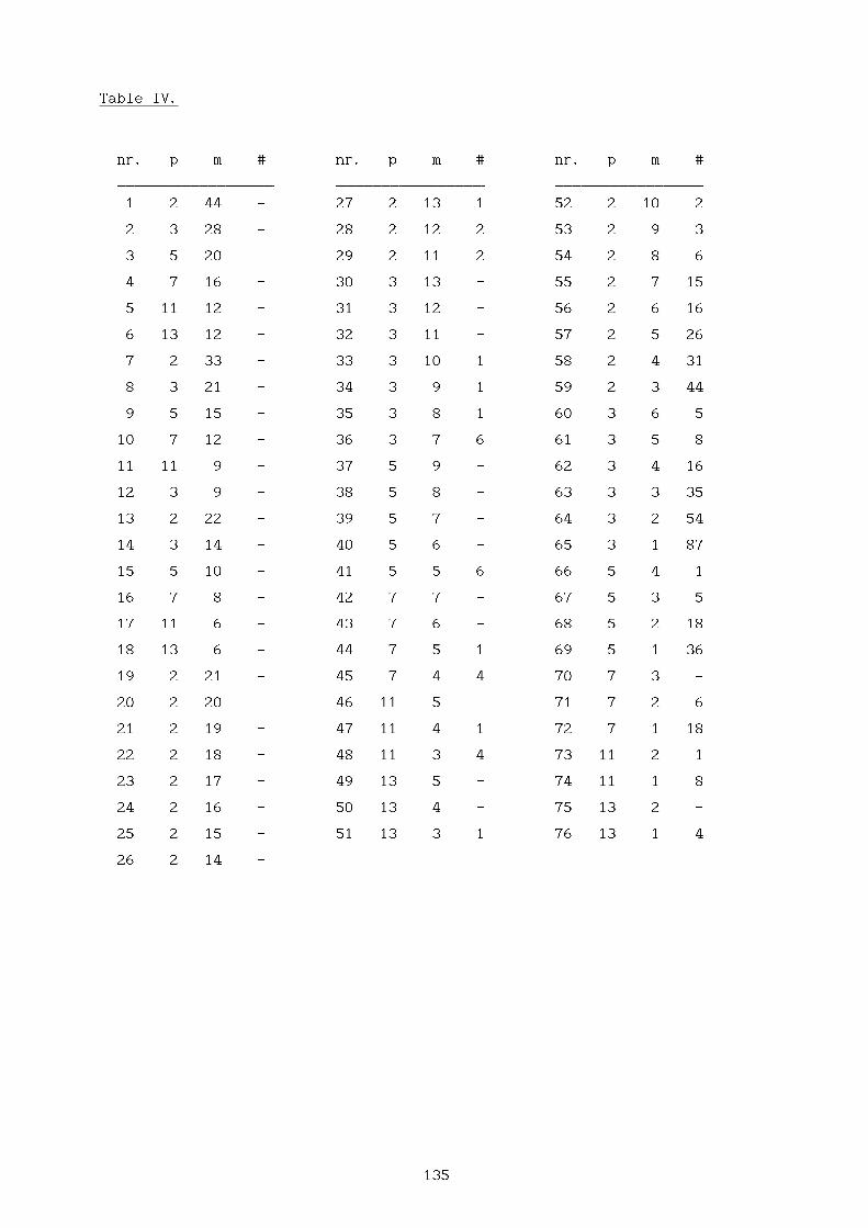
Table_IV.

nr. p m # nr. p m # nr. p m #

------------------------------------------------------------------------------------------ ------------------------------------------------------------------------------------- -------------------------------------------------------------------------------------1 2 44 - 27 2 13 1 52 2 10 2

2 3 28 - 28 2 12 2 53 2 9 3

3 5 20 - 29 2 11 2 54 2 8 6

4 7 16 - 30 3 13 - 55 2 7 15

5 11 12 - 31 3 12 - 56 2 6 16

6 13 12 - 32 3 11 - 57 2 5 26

7 2 33 - 33 3 10 1 58 2 4 31

8 3 21 - 34 3 9 1 59 2 3 44

9 5 15 - 35 3 8 1 60 3 6 5

10 7 12 - 36 3 7 6 61 3 5 8

11 11 9 - 37 5 9 - 62 3 4 16

12 3 9 - 38 5 8 - 63 3 3 35

13 2 22 - 39 5 7 - 64 3 2 54

14 3 14 - 40 5 6 - 65 3 1 87

15 5 10 - 41 5 5 6 66 5 4 1

16 7 8 - 42 7 7 - 67 5 3 5

17 11 6 - 43 7 6 - 68 5 2 18

18 13 6 - 44 7 5 1 69 5 1 36

19 2 21 - 45 7 4 4 70 7 3 -

20 2 20 - 46 11 5 - 71 7 2 6

21 2 19 - 47 11 4 1 72 7 1 18

22 2 18 - 48 11 3 4 73 11 2 1

23 2 17 - 49 13 5 - 74 11 1 8

24 2 16 - 50 13 4 - 75 13 2 -

25 2 15 - 51 13 3 1 76 13 1 4

26 2 14 -

135

Chapter 7. The sum of two S-units being a square.

7.1. Introduction.

Let p , ..., p ( s > 1 ) be distinct primes, and let S be the set of1 s

positive rational integers which have no prime divisors different from the

p . A rational number is called an S-unit if its absolute value is aiquotient of elements of S . Thus the set of S-units is

x x1 s

{ + p W...Wp | x e Z for i = 1, ..., s } .1 s i

We study the diophantine equation

2x + y = z

in S-units x, y , and z e Q , where the set of primes p , ..., p is1 s

given. We show how to find all solutions of this equation, using the theory

of p-adic linear forms in logarithms, and a computational p-adic diophantine

approximation method. We actually perform all the necessary computations for

solving the equation completely for { p , ..., p } = { 2, 3, 5, 7 } . This1 s

type of equations has applications in arithmetic algebraic geometry (cf.

Setzer [1975], Pinch [1984]).

We start with getting rid of the denominators. Let x, y, z be a solution.2

There is a d e S such that |dWx|, |dWy| e S . Put d = d Wd , where1 2

d , d e S and d squarefree. Then1 2 1

2d WdWx + d WdWy = (d Wd Wz) ,1 1 1 2

2which has the same form as x + y = z , but now |d WdWx|, |d WdWy| e S C Z

1 1and d Wd Wz e Z . Without loss of generality we may therefore study

1 2

2x + y = z , (7.1)

where

(x e S , +y e S , z e Z ,

|{ x > y , z > 0 , (7.2)|7 (x,y) is squarefree .

136

We shall prove the following results.

THEOREM_7.1. Let p , ..., p be given. There exists an effectively1 s

computable constant C , depending on p , ..., p only, such that any1 s

solution x, y, z of equation (7.1) with conditions (7.2) satisfies

max (x,|y|,z) < C .

THEOREM_7.2. Let { p , ..., p } = { 2, 3, 5, 7 } . Equation (7.1) with1 s

conditions (7.2) has exactly the 388 solutions given in Table I.

Remarks. 1. The Tables are given in Section 7.9. We stress that the aim of

this chapter is not only to prove these theorems, but to show as well that

for any given set of primes { p , ..., p } a result similar to Theorem 7.21 s

can be proved along the same lines, in a more or less algorithmic way.

2. Equation (7.1) with conditions (7.2) can be seen as a further

generalization of the generalized Ramanujan-Nagell equation

n n2 1 sx + k = p W...Wp , (7.3)

1 s

(cf. Chapter 4), namely by taking |k| e S arbitrary instead of k e Z

fixed. The method of this chapter to solve (7.1) is also a generalization of

the method of Chapter 4 to solve (7.3).

Equation (7.1) can be transformed into a number of Pell-like equations. Put

2x = DWu ,

swhere D, u e S , and D is squarefree. There are only 2 possibilities

for D . Now, (7.1) is equivalent to a finite number of equations

2 2z - DWu = y (7.4)

in u e S , +y e S , z e Z , with z > 0 and (u,y) = 1 . We treat

equation (7.4) by factorizing its both sides in the field K = Q(rD) . When

dealing with equation (7.4) we allow z and u to be negative.

7.2. The case D = 1 .

First we consider the special case D = 1 . Then (7.4) is equivalent to

137

& z + u = y1

{ ,7 z - u = y

2

where y = y Wy , y e S , +y e S , and y > |y | . Subtraction yields1 2 1 2 1 2

2Wu = y - y , (7.5)1 2

where now all variables u, y , y (apart from the sign) are in S , hence1 2

in Z . By (u,y ) = (u,y ) = 1 , equation (7.5) is of the form a + b = c ,1 2

or 2Wa + 2Wb = 2Wc , where a, b, c are composed of primes 2, p , ..., p1 s

only, and (a,b) = 1 , a > b > 0 . In Chapter 6 it was shown how to solve

a + b = c . For our standard example { p , ..., p } = { 2, 3, 5, 7 } we1 s

have the following result.

LEMMA_7.3. Let { p , ..., p } = { 2, 3, 5, 7 } . Equation (7.1) with1 s

conditions (7.2) and D = 1 has exactly the 95 solutions given in Table I

with D = 1 .

Proof. From Theorem 6.3 it follows that a + b = c with a, b, c e S ,

(a,b) = 1 , a > b has exactly 63 solutions. They are easy to compute. Each

of these gives rise to three possibilities for (7.5):

1if 2 | a then (u,y ,y ) = (-----a,b,c), (b,2c,2a), (c,2a,-2b),

1 2 2

1if 2 | b then (u,y ,y ) = (a,2b,2c), (-----b,c,a), (c,2a,-2b),

1 2 2

1if 2 | c then (u,y ,y ) = (a,2b,2c), (b,2c,2a), (-----c,a,-b).

1 2 2

Of the thus found 189 possibilities, the 95 ones given in Table I with D = 1

satisfy x > y and z > 0 , whereas the others don’t. p

This completes our treatment of the case D = 1 .

7.3. Towards generalized recurrences.

From now on, let D > 1 . Put K = Q(rD) . Let s : K -----L K be the

automorphism of K with s(rD) = -rD . For any number or ideal X in K we

write X’ for s(X) , for convenience. Let p for i = 1, ..., s be thei

prime ideal in K such that ord (p ) > 0 . If p splits in O , this isp i i Ki

well defined if a choice has been made from the two possibilities for

rD (mod p ) . Put for a solution z, u, y of (7.4)

138

c = z + uWrD .

Then y = cWc’ , and by (u,y) = 1 we have

( )min ord (u), ord (y) = 0 . (7.6)

9 p p 0i i

Equation (7.4) leads to the conjugated ideal equations

( s a bi i

| (c) = p p Wp’i i

| i=1{ (7.7)| s a b

i i| (c’) = p p’ Wp

i i9 i=1

where a , b e N , and b = 0 if p = p’ . We need the followingi i 0 i i i

auxiliary lemma.

LEMMA_7.4. If x e K and ord (x) = ord (x’) for a prime p , thenp p

ord (x) < ord (x-x’) .p p

Moreover, if p = 2 and D _ 1 (mod 8) , then

ord (x) < ord ((x-x’)/2) ,2 2

and, if p = 2 and D _ 2, 3 (mod 4) , then

1ord (x) < ord ((x-x’)/2rD) + ----- .

2 2 2

Proof. This is an easy exercise, which we leave to the reader. p

We distinguish, as usual, three cases for the factorization of the prime pi

in K : it may split, ramify or remain prime. See Borevich and Shafarevich

[1966], section III.8.

-----L p remains prime in K . Then p ! D , and if p = 2 theni i i

D _ 5 (mod 8) . We have (p ) = p = p’ , and from ord (c) = ord (c’) andi i i p p

i iLemma 7.4 we obtain

ord (y) = 2Word (c) < 2Word (c-c’) = 2Word (2WuWrD) .p p p pi i i i

It follows, using (7.6), that

139

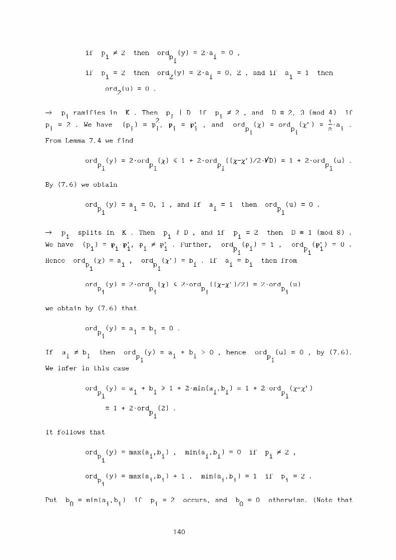
if p $ 2 then ord (y) = 2Wa = 0 ,i p i

i

if p = 2 then ord (y) = 2Wa = 0, 2 , and if a = 1 theni 2 i i

ord (u) = 0 .2

-----L p ramifies in K . Then p | D if p $ 2 , and D _ 2, 3 (mod 4) ifi i i

2 1p = 2 . We have (p ) = p , p = p’ , and ord (c) = ord (c’) = -----Wa .i i i i i p p 2 i

i iFrom Lemma 7.4 we find

ord (y) = 2Word (c) < 1 + 2Word ((c-c’)/2WrD) = 1 + 2Word (u) .p p p pi i i i

By (7.6) we obtain

ord (y) = a = 0, 1 , and if a = 1 then ord (u) = 0 .p i i pi i

-----L p splits in K . Then p ! D , and if p = 2 then D _ 1 (mod 8) .i i i

We have (p ) = p Wp’, p $ p’ . Further, ord (p ) = 1 , ord (p’) = 0 .i i i i i p i p i

i iHence ord (c) = a , ord (c’) = b . If a = b then from

p i p i i ii i

ord (y) = 2Word (c) < 2Word ((c-c’)/2) = 2Word (u)p p p pi i i i

we obtain by (7.6) that

ord (y) = a = b = 0 .p i ii

If a $ b then ord (y) = a + b > 0 , hence ord (u) = 0 , by (7.6).i i p i i p

i iWe infer in this case

ord (y) = a + b > 1 + 2Wmin(a ,b ) = 1 + 2Word (c-c’)p i i i i pi i

= 1 + 2Word (2) .pi

It follows that

ord (y) = max(a ,b ) , min(a ,b ) = 0 if p $ 2 ,p i i i i ii

ord (y) = max(a ,b ) + 1 , min(a ,b ) = 1 if p = 2 .p i i i i ii

Put b = min(a ,b ) if p = 2 occurs, and b = 0 otherwise. (Note that0 i i i 0

140

min(a ,b ) = 1 may occur only if p $ p’ , hence only if p = 2 splits).i i i i i

Let us assume that the splitting primes of p , ..., p are p , ..., p1 s 1 t

for some 0 < t < s . Put

I = { i | 1 b } ,i i

I’ = { i | 1 < i < t , a < b } .i i

hi

For i = 1, ..., t , let h be the smallest positive integer such that pi i

is a principal ideal, say

hi

p = (p ) .i i

If h denotes the class number of K , then h | h . Now, p e K isi i

determined up to multiplication by a unit. Thus we may choose p such thati

|p | > |p’| if i e I ,i i

|p | < |p’| if i e I’ .i i

For i = 1, ..., t , put

| a - b | = c Wh + d ,i i i i i

with c , d e N , and 0 < d < h - 1 . Consider the ideali i 0 i i

b d d s a0 i i i

a = (2) W p p W p p’ W p p .i i i

ieI ieI’ i=t+1

From the above considerations it follows that, for given K , p , ..., p ,1 s

there are only finitely many possibilities for a . By (7.7) it follows that

c ci i

(c) = aW p (p ) W p (p’)i i

ieI ieI’

(namely, |a -b | = max(a ,b ) if p $ 2 , since then min(a ,b ) = 0 ; andi i i i i i i

|a -b | = max(a ,b ) - 1 if p = 2 and b = 1 ). Hence a is a principali i i i i 0

ideal, say

a = (a)

for an a e O . Up to multiplication by a unit, there are only finitely manyK

possibilities for a . Let e be the fundamental unit of K with e > 1 .

141

Now, (7.7) leads to the system of equations

c cn i i

& c = z + urD = +a W e W p p W p p’i i

| ieI ieI’{ , (7.8)

c c| n i i

c’ = z - urD = +a’We’ W p p’ W p p7 i i

ieI ieI’

where n e Z . Put for n e Z , m , ..., m e N , and for each possible a1 t 0

m m m ma n i i a’ n i i

G (n,m ,...,m ) = ---------------We W p p W p p’ - ---------------We’ W p p’ W p p ,a 1 t 2rD i i 2rD i i

ieI ieI’ ieI ieI’

m m m ma n i i a ’ n i i

H (n,m ,...,m ) = ----- We W p p W p p’ + ----- We’ W p p’ W p p .a 1 t 2 i i 2 i i

ieI ieI’ ieI ieI’

Then (7.8) is equivalent to

& + u = G (n,c ,...,c )a 1 t

{ . (7.9)7 + z = H (n,c ,...,c )

a 1 t

The functions G and H are generalized recurrences in the sense that ifa a

all variables but one are fixed, then they become integral binary recurrence

sequences. We show an example in Fig. 8.

a n m a’ n mFigure_8. G (n,m) = ---------------We Wp - ---------------We’ Wp’ for D = 30, a = 5 + r30,

a 2rD 2rDe = 11 + 2Wr30, p = 13 + 2Wr30 , with -10 < n < 10 (vertically) and

120 < m < 10 (horizontally). Numbers > 10 are denoted by asterisks.

7.4. Towards linear forms in logarithms.

Let us write u = ord (u) for i = 1, ..., s . Put for each ai p

i

142

bdeweger

Stamp

I = { i | 1 0 occursU p a 1 t

it

for at least one (n,m ,...,m ) e Z * N } .1 t 0

Note that since (u,y) = 1 the sets I , I, I’ are disjunct. We proceedU

with the first equation of system (7.9). Written out in full detail it reads

c c c c ua n i i a’ n i i i

---------------We W p p W p p’ - ---------------We’ W p p’ W p p = + p p . (7.10)2rD i i 2rD i i i

ieI ieI’ ieI ieI’ ieIU

Now, I, I’, I depend on a , which depends on the particular solution ofU

equation (7.4) that we presupposed. However, we know that a belongs to a

finite set, which can be computed explicitly. So if we can solve (7.10)

completely for each a of this set, then we can find all solutions of (7.9),

hence of (7.1).

The set of the a’s may be reduced, without loss of generality, as follows.

If D _ 1 (mod 8) then b = 0, 1 may both occur, with a = a , 2Wa0 0 0

respectively. We only have to consider 2Wa , because if u = u , z = z is0 0 0

a solution of (7.9) for a = a , then u = 2Wu , z = 2Wz is a solution of0 0 0

(7.9) for a = 2Wa . Hence it is not necessary to consider a = a if also0 0

a = 2Wa is already being considered. By the same argument, if0

D _ 5 (mod 8) then with a = a such that ord (a ) = 0 also a = 2Wa0 2 0 0

may occur, so that we only have to consider the latter. Note that it may now

occur that (u,y) = 2 . The condition (u,y) = 1 is used only to ensure that

I and I u I’ are disjunct. This remains true in the above cases withU(u,y) = 2 . Further, if (a ) $ (a’) for some a , then we only have to

0 0 0consider one a of the pair a , a’ . Namely, if the I, I’ belonging to

0 0a are I , I’ , then the I, I’ belonging to a’ are I’, I , and then0 0 0 0 0 0

a’ c c a c c0 n i i 0 n i i

G (n,m ,...,m ) = ---------------We Wp p Wp p’ - ---------------We’ Wp p’ Wp pa’ 1 t 2rD i i 2rD i i0 I’ I I’ I

0 0 0 0

& a’ c c a c c *0 -n i i 0 -n i i

= + | ---------------We’ Wp p’ Wp p - ---------------We Wp p Wp p’ |2rD i i 2rD i i

7 I I’ I I’ 80 0 0 0

= - G (-n,m ,...,m ) ,a 1 t0

(by using eWe’ = +1 ), and analogously

H (n,m ,...,m ) = + H (-n,m ,...,m ) .a’ 1 t a 1 t0 0

143

From equation (7.10) we now derive p -adic linear forms in logarithms, ini

three different ways, according to i e I, I’ or I . PutU

3 1g = ----- if p = 2 , g = 1 if p = 3 , g = ----- if p > 5 .i 2 i i i i 2 i

Then g > 1/(p -1) , hence if ord (x) > g for a x e K theni i p i

i

ord (log (1+x)) = ord (x) . (7.11)p p pi i i

We now have the following result.

LEMMA_7.5. Let n, c ( i e I u I’ ) , u ( i e I ) satisfy (7.10).i i U

(i). For i e I putU

l = ord (2rD/a’) ,i p

i

pa e j

L = log (----------) + nWlog (----------) + S c Wlog (----------)i p a’ p e’ j p p’

i i jeI i j

pj

- S c Wlog (----------) .j p p’

jeI’ i j

If u + l > g theni i i

u + l = ord (L ) .i i p i

i

(ii). For i e I put

ak = ord (----------) ,i p a’

i

a’K = log (---------------) + nWlog (e’) - S u Wlog (p )i p 2rD p j p j

i i jeI iU

+ S c Wlog (p’) + S c Wlog (p ) .j p j j p j

jeI i jeI’ i

If h Wc + k > g theni i i i

h Wc + k = ord (K ) .i i i p i

i(ii’). For i e I’ put

a’k’ = ord (----------) ,i p a

i

144

aK’ = log (---------------) + nWlog (e) - S u Wlog (p )i p 2rD p j p j

i i jeI iU

+ S c Wlog (p ) + S c Wlog (p’) .j p j j p j

jeI i jeI’ i

If h Wc + k’ > g theni i i i

h Wc + k’ = ord (K’) .i i i p i

i

Remark. Note that all the above p -adic logarithms are well-defined, sincei

their arguments have p -adic order zero. This follows from the fact that I ,i U

I and I’ are disjunct, and if D _ 1 (mod 8) from the choice a = 2Wa .0

Proof. For (i), divide (7.10) by its second term. For (ii), divide (7.10) by

its second term, and add 1. For (ii’), divide (7.10) by its first term, and

add -1. Then in all three cases take the p -adic order, and apply (7.11). pi

The linear forms in logarithms L , K , K’ , as they appear in Lemma 7.5,i i i

seem to be inhomogeneous, since the first term has coefficient 1. However, it

can be made homogeneous by incorporating this first term in the other ones,

as follows. Put

*h = lcm ( 2, h , ..., h ) .

1 s

Note that, by the definition of a ,

** n n n s n h Wbh 0 i i i 0a = + e W p p W p p’ W p p W2 , (7.12)

i i iieI ieI’ i=t+1

where the exponents n for 0 < i < s are integral. It follows thati

*h n n n

&a * &e * 0 &p * i &p’* i---------- = + ---------- W p ---------- W p ---------- .7a’8 7e’8 7p’8 7p 8

ieI ieI’

Put

* * * * * *L = h WL , n = h Wn + n , c = h Wc + n .i i 0 j j j

Then it follows that

p p* * e * j * jL = n Wlog (----------) + S c Wlog (----------) - S c Wlog (----------) .i p e’ j p p’ j p p’

i jeI i j jeI’ i j

145

Note that the prime divisors of D are just the ramifying primes. By (7.12),

* *h n n n s n -n h W(b -n )

a 0 i i i i 0 0(---------------) = + e W p p W p p’ W p p W2 ,2rD i i i

ieI ieI’ i=t+1

1 *where n = -----Wh Word (4D) e Z for i = t+1, ..., s , and n = 1 if 2

i 2 p 0i

splits, n = 0 otherwise. If p = 2 splits we have assumed that b = 1 .0 i 0

Hence the last factor vanishes. So put

* * * * * *K = h WK , K’ = h WK’ , u = h Wu - ( n - n ) ,i i i i j j j j

*I = I u { i | t+1 < i < s , n $ 0 } .U U i


* * * *K = n Wlog (e’) - S u Wlog (p ) + S c Wlog (p’) +i p * j p j j p j

i jeI i jeI iU

*+ S c Wlog (p ) ,

j p jjeI’ i

* * * *K’ = n Wlog (e) - S u Wlog (p ) + S c Wlog (p ) +i p * j p j j p j

i jeI i jeI iU

*+ S c Wlog (p’) .

j p jjeI’ i

This leads to the following reformulation of Lemma 7.5.

LEMMA_7.6. Let n, c for i e I u I’ , u for i e I be a solution ofi i U

* * * * *(7.10), let l , k , k’ be as in Lemma 7.5, and let h , L , K , K’ , n ,

i i i i i i i* * *c , u , I be as above.i i U(i). Let i e I . If u + l > g then

U i i i

* *u + l + ord (h ) = ord (L ) .i i p p i

i i

(ii). Let i e I . If h Wc + k > g theni i i i

* *h Wc + k + ord (h ) = ord (K ) .i i i p p i

i i

(ii’). Let i e I’ . If h Wc + k’ > g theni i i i

* *h Wc + k’ + ord (h ) = ord (K’ ) .i i i p p i

i i

146

* * *Remark. We will study the linear forms in logarithms L , K , K’ for

i i i* * *

arbitrary integral values of the variables n , c , u . Notice that thei i

parameter a has disappeared completely from these linear forms. This means

that we have to consider the linear forms for each D only, instead of for

each a .

7.5. Upper bounds for the solutions: outline.

Let us first give a global explanation of our application of the theory of

p-adic linear forms in logarithms, that gives explicit upper bounds for the* * *

variables occurring in the linear forms L , K , K’ . Then we give argumentsi i i

why we choose this way to apply the theory, and not other possible ways. In

the next section we give full details of the derivation of the upper bounds.

In the sequel, by the ’constants’ C , ..., C we mean numbers that depend1 12

only on the parameters of (7.10), not on the unknowns n, c , u .i i

Put

M = max (c ) , U = max (u ) , B = max ( M, U, |n| ) ,i i

ieIuI’ ieIU

* * * * * * * *M = max (c ) , U = max (u ) , B = max ( M , U , |n | ) ,

i iieIuI’ ieI

U

N = max ( |n |, ..., |n |, |n -n |, ..., |n -n | ) .0 t t+1 t+1 s s


** * X + NX < h WX + N , X < ------------------------------ (7.13)

*h

for X = M, U, B . We apply Lemma 2.6 to the p-adic linear forms in*

logarithms. For L we find, in view of Lemma 7.6(i),i

*U < C + C Wlog(B ) , (7.14)

1 2

* *and for K , K’ we find, in view of Lemma 7.6(ii),(ii’),

i i

*M < C + C Wlog(B ) . (7.15)

3 4

Here, C , C , C , C are constants that can be written down explicitly. In1 2 3 4

order to find an upper bound for B we try to find C , C such that10 11

147

*B < C + C Wlog(B ) . (7.16)

10 11

In view of (7.13) we may insert and delete asterisks any time we like, as

long as we don’t specify the constants. In order to prove (7.16) it remains,

in view of (7.14) and (7.15), to bound |n| by a constant times log B . We

will introduce certain constants C , C , C , and distinguish three cases:5 6 7

(a). - ( C + C WM ) < n < C ,6 7 5

(b). n > C , (7.17)5

(c). n < - ( C + C WM ) .6 7

In case (a) it is, by (7.15), obvious that (7.16) holds. In cases (b) and (c)

one of the two terms of G dominates. We shall show that there exista

constants C , C such that8 9

|n| < C + C WU . (7.18)8 9

Then (7.16) follows from (7.14).

From (7.16) we derive immediately an explicit upper bound C for B ,12

hence for all the variables involved. Since the constants C , ..., C will1 4

be very large, also C will be very large. To find all solutions we12

proceed by reducing this upper bound, by applying the computational p-adic

diophantine approximation technique described in Section 3.11, to the p-adic* * *

linear forms in logarithms L , K , K’ . Crucial in that line of argument isi i i

that the constants C , ..., C are very small compared to C , ..., C .5 9 1 4

This method leads to reduced bounds for the p-adic orders of the linear

forms. Then we can replace (7.14) and (7.15) by much sharper inequalities,

and repeat the above argument, to find a much sharper inequality for (7.16).

In general we expect that it is in this way possible to reduce in one step

the upper bound C for B to a reduced bound of size log C .12 12

Before going into detail we explain briefly that it is possible to treat

(7.10) partly by the theory of real (instead of p-adic) linear forms in

logarithms, and subsequently by a real computational diophantine

approximation technique (cf. Section 3.7), and why we prefer not to do so.

First, note that K and K’ have generically more terms than L , and arei i i

therefore more complicated to handle. Since K , K’ occur only in case (a),i i

this is the most difficult case. Equation (7.10) consist of three terms, each

of which is purely exponential, i.e. the bases are fixed and the exponents

are variable. If one of these three terms is essentially smaller than the

148

other two (more specifically, smaller than the other terms raised to the

power d , for a fixed d e (0,1) ), then we can apply the real method. There

are two ways of doing this. Write (7.10) as

c - c’ = 2WuWrD .

dFirst, suppose that |c-c’| < |c’| . Then |n| cannot be very large, and we

are essentially (i.e. apart from a finite domain) in case (a). Unfortunately,

the region for |n| that we can cover in this way becomes smaller as M -----L 81/d

(see the example below). Second, suppose that |c| > |c’| , ord

|c| < |c’| . Then we are essentially in case (b) or (c). But this area can

be dealt with easier p-adically, since here we use the linear forms L ,i

whereas the real linear forms in logarithms used in this case will

generically have more terms. The areas sketched above, in which we can apply

the real theory, will not cover the whole domain corresponding to case (a)

(cf. the white regions in Fig. 9 below). Hence we cannot avoid working with

the p-adic linear forms K , K’ . But then it is more convenient to avoid thei i

use of real linear forms.

Figure_9.

149

bdeweger

Stamp

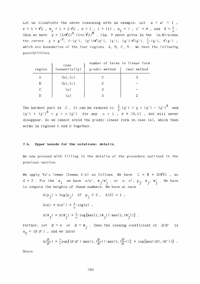
Let us illustrate the above reasoning with an example. Let a = a’ = 1 ,1

e = 1 + r2 , p = 1 + 2Wr2 , s = 1 , I = {1} , p = 7 , I’ = o , and d = ----- .1 1 2

n MThen we have c = (1+r2) W(1+2Wr2) . Fig. 9 above gives in the (n,M)-plane

2 1the curves c = c’ , 2W|c’|, |c’|+r|c’|, |c’|, |c’|-r|c’|, -----W|c’|, r|c’| ,

2

which are boundaries of the four regions A, B, C, D . We have the following

possibilities.

number of terms in linear form| case |

region | (essentially) 1 p-adic method 1 real method---------------------------------------------k---------------------------------------------------------------------------k-------------------------------------------------------------------------------------k----------------------------------------------------------------------

A 1 (b),(c) 1 2 1 31

1 1B (b),(c) 2 1 -

1 11

C 1 (a) 1 3 -1

1 1D 1 (a) 1 3 1 2

1 dThe hardest part is C . It can be reduced to -----W|c’| < c < |c’| - |c’| and

cd

|c’| + |c’| < c < cW|c’| for any c > 1 , d e (0,1) , but will never

disappear. So we cannot avoid the p-adic linear form in case (a), which then

works in regions C and D together.

7.6. Upper bounds for the solutions: details.

We now proceed with filling in the details of the procedure outlined in the

previous section.

We apply Yu’s lemma (Lemma 2.6) as follows. We have L = K = Q(rD) , so

d = 2 . For the a we have e/e’, p /p’ , or e, e’, p , p , p’ . We havei j j j j j

to compute the heights of these numbers. We have at once

h(p ) = log(p ) if p > 3 , h(2) = 1 ,j j j

1h(e) = h(e’) = -----Wlog(e) ,

2

1 ( )h(p ) = h(p’) = -----Wlog max(1,|p |)Wmax(1,|p’|) .

j j 2 9 j j 0

Further, let b = e or b = p . Then the leading coefficient of b/b’ isj

a = |bWb’| , and we infer0

b 1 ( b b’ ) ( )h(----------) = -----log |bWb’|Wmax(1,|----------|)Wmax(1,|----------|) = log max(|b|,|b’|) .b’ 2 9 b’ b 0 9 0

Hence

150

pe j ( )

h(----------) = log(e) , h(----------) = log max(|p |,|p’|) .e’ p’ 9 j j 0

j

The order of the a is important in two respects: it is required that thei

V for i = 1, ..., n-1 are in increasing order, and that ord (b ) isi p nminimal among the ord (b ) . Since the b are the unknowns, we should

p i iassume that V < V < ... < V . In the final bound however, only the

n 1 n-1+

product V W...WV and V appear. So the ordering of the V only1 n n-1 i

+matters for defining V . It follows that we can take

n-1

( )V = max h(a ), f W(log p)/d ,i 9 i p 0

with the a in any order, if we definei

+V = max ( 1, V , ..., V ) .n-1 1 n

Further, we take

f /d( 4 p )

B = B = B = B’ = max |b |, ..., |b |, 2, -----WnW(p -1) .0 n 9 1 n 3 0

3 3Then log(1+----------WB) > f W(log p)/d . By B > 2 it follows that 1 + ----------WB < B .

4n p 4nHence we can take

W = log B .

There are two more conditions to be checked. The first one is thatb b1 n

a W...Wa $ 1 . This is immediate, if we assume the obvious condition that1 n

1/q 1/q nnot all b are zero. The second one is [K(a ,...,a ):K] = q , which

i 1 nis less obvious. For our situation it follows from the following lemma.

Application of Yu’s newest results avoids such a condition (cf. Yu [1989]).

Nevertheless we include the lemma here, to show that it is often possible to

prove such a condition, which may in some cases lead to lower constants.

LEMMA_7.7. Let K = Q(rD) , with e as fundamental unit, and h as class

number. Let p , ..., p be distinct prime numbers, and let p be for1 s i

i = 1, ..., s a prime ideal in K lying above p . Let h be a divisori i

hi

of h such that p is principal, and denote a generator by p . Leti i

either: (1) all p split, and theni

pe j

x = ---------- , x = ---------- for i = 1, ..., s ,0 e’ j p’

j

151

or: (2)

x = e or e’ , x = p or p’ for j = 1, ..., s .0 j j j

Let q be an odd prime, not dividing h . Then

1/q 1/q s+1[K(x ,...,x ):K] = q .

0 s

1/q 1/qProof. Let K = K(x ) , and K = K (x ) for i = 1, ..., s . We use

0 0 i i-1 is+1

induction on i to prove that [K :K] = q . Note that [K :K] = q .s 0

i+1Suppose that [K :K] = q . It remains to prove that [K :K ] = q , hence

i i+1 iit suffices to prove that x m K , since q is prime. Suppose the

i+1 ii+1

contrary is true. K is a K-vector space of dimension q , with asi

basis all the elements

i k /qj

t = p xk ,...,k j0 i j=0

for k e { 0, 1, ..., q-1 } for j = 0, ..., i . It follows that therej

exist a e K such thatk ,...,k0 i

1/qx = S a Wt . (7.19)i+1 k ,...,k k ,...,k

k ,...,k 0 i 0 i0 i

The group of K-embeddings of K into C is generated by the s fori j

j = 0, ..., i defined by

1/q 1/qs (x ) = x for l = 0, ..., i , l $ j ,j l l

1/q 1/qs (x ) = rWx ,j j j

where r is a primitive q th root of unity. Hence all the embeddings are

given by

i lj

v = p sl ,...l j0 i j=0

for l e { 0, 1, ..., q-1 } . It follows thatj

i l i k /q i l kj( m ) j j

v (t ) = p s p x = p r Wtl ,...,l k ,...,k j 9 m 0 k ,...,k0 i 0 i j=0 m=0 j=0 0 i

152

iS l k

j jj=0

= r Wt .k ,...,k0 i

1/q qThe minimal polynomial of x over K is X - x . Hence the

i+1 i+11/q j 1/q

conjugates of x are r Wx for j = 0, 1, ..., q-1 , all with equali+1 i+1

multiplicity. There exist numbers m e { 0, 1, ..., q-1 } such that forj

j = 0, 1, ..., q-1 we have

m1/q j 1/q

s (x ) = r Wx .j i+1 i+1

HenceiS l m

j j1/q j=0 1/q

v (x ) = r Wx .l ,...,l i+1 i+10 i

Now apply v to (7.19). Then for each tuple (l ,...,l ) we findl ,...,l 0 i0 i

i iS l m S l k

j j j jj=0 1/q j=0r Wx = S a Wr Wt .

i+1 k ,...,k k ,...,kk ,...,k 0 i 0 i0 i

i+1 i+1Here we have a system of q linear equations in the q unknowns

a . The determinant of this system is exactly the square root of thek ,...,k0 i

i+1q

discriminant of K over K , hence nonzero. Consequently there is in Ci

just one solution of the system. But we know that solution:

a = 0 if (k ,...,k ) $ (m ,...,m ) ,k ,...,k 0 i 0 i0 i

1/q -1a = x Wt .m ,...,m i+1 m ,...,m0 i 0 i

The latter equation now yields an equation over K :

i mq j

x = a W p x .i+1 m ,...,m j

0 i j=0

In case (1) this leads to the ideal equation

h m Wh&p * i+1 i &p * j ji+1 q j

|--------------------| = a W p |----------| ,p’ p’7 i+18 j=17 j8

153

and in case (2) to

h i m Wh(’) i+1 q (’) j jp = a W p p ,i+1 j

j=1

(’)(where p stands for p or p’ ) for some fractional ideal a (note

that (x ) = (1) ). Because of unique factorization for ideals it follows in0

both cases that q divides all m Wh for j = 1, ..., i and h . Thisj j i+1

contradicts the assumption q ! h . p

b b1 n

Remarks. 1. If ord (a W...Wa -1) > 1/(p-1) thenp 1 n

b b1 n

ord (a W...Wa -1) = ord (b Wlog (a )+...+b Wlog (a )) .p 1 n p 1 p 1 n p n

We prefer to work with the logarithmic version, since that is the one we use

in the computational method of reducing the upper bounds.

2. In order to apply Yu’s lemma we can take for q the smallest odd primefp

that does not divide hWpW(p -1) .

3. The author is grateful to M.A.J.G. van der Vlugt (Leiden) for discussions

on the above lemma.

We now proceed to compute the constants C to C . To find C and C1 12 1 2

*we apply Lemma 2.6 to L , for all i e I . Then we find for each such i

i Uconstants C , C such that, under the conditions

1,i 2,i

f /2p

* ( 4 i )u + l > g , B > max 2, -----Wt W(p -1) ,i i i 9 3 i i 0

*(where t denotes the number of terms in L ), we obtain

i i

* *ord (L ) < C + C Wlog B .

p i 1,i 2,ii

By Lemma 7.6(i) and the relation ord = e Word , and assuming thatp p p

f /2p

* ( 4 i )U > max (g -l ) , B > max 2, -----Wt W(p -1) , (7.20)

i i 9 3 i i 0ieI ieI

U U

we see that it suffices to take

( * )C = max -(l +ord (h )) + C /e , C = max ( C /e ) .1 9 i p 1,i p 0 2 2,i p

ieI i i ieI iU U

Then (7.14) holds.

154

* *Next we apply Lemma 2.6 to K and K’ , for all i e I and I’

i i(’)

respectively, to obtain C and C . By X we denote X if i e I ,3 4

and X’ if i e I’ . There exist by Lemma 2.6 constants C and C3,i 4,i

such that under the conditions

f /2p

(’) * ( 4 i )h Wc + k > g , B > max 2, -----Wt W(p -1)i i i i 9 3 i i 0

(’)*(where again t denotes the number of terms of K ), it follows that

i i

(’)* *ord (K ) < C + C Wlog B .

p i 3,i 4,ii

Again, by Lemma 7.6(ii),(ii’) it follows that, under the conditions

(’) f /2g -k p( i i ) * ( 4 i )

M > max ----------------------------------- , B > max 2, -----Wt W(p -1) (7.21)9 h 0 9 3 i i 0

ieIuI’ i ieIuI’

it suffices to take

(’) *k +ord (h )i p C C

( i 3,i ) ( 4,i )C = max ----------------------------------------------------------------------- + ------------------------------ , C = max ------------------------------ .3 9 h h We 0 4 9h We 0

ieIuI’ i i p ieIuI’ i pi i

Then (7.15) holds.

We take C to C as follows:5 7

|a’| |a |C = log(2W|----------|)/2Wlog e , C = log(2W|----------|)/2Wlog e ,5 |a | 6 |a’|

|p | |p’|( | i| | i| )

C = S log|----------| + S log|----------| /2Wlog e .7 9 |p’| |p | 0

ieI | i| ieI’ | i|

Note that C or C may be negative, but that always -C < C . Further,5 6 6 5

C is always strictly positive, unless I = I’ = o . Next we show how to7take C and C . Suppose first that

8 9

n > max ( C , 0 ) .5

Then, from eWe’ = +1 and the choice of p we find by (7.8) thati

c cn |p | i |p’| i

|c | |a | |e | | i| | i| |a | 2Wn|----------| = |----------|W|----------| W p |----------| W p |----------| > |----------|We > 2 ,|c’| |a’| |e’| |p’| |p | |a’|

ieI| i| ieI’| i|

which expresses that the first term of G dominates. Puta

155

P = p p .i

ieIU

Then we infer

uU iP > p p = |c-c’|/2WrD > |c|/4WrD

iieI

U

c c|a| n i i |a| n

= ---------------We W p |p | W p |p’| > ---------------We ,4rD i i 4rD

ieI ieI’

hence

( 4rD )n < log(---------------) + UWlog(P) /log e .

9 |a| 0

Next suppose that

n < min ( -(C +C WM), 0 ) .6 7

Then we find that the second term of G dominates, namelya

c cn |p’| i |p | i

|c’| |a’| |e’| | i| | i||----------| = |----------|W|----------| W p |----------| W p |----------||c | |a | |e | |p | |p’|

ieI| i| ieI’| i|

M& |p’| |p |* -2W(n+C WM)

|a’| -2Wn | i| | i| |a’| 7> |----------|We W| p |----------|W p |----------|| = |----------|We|a | |p | |p’| |a |

7ieI| i| ieI’| i|8

2WC|a’| 6

> |----------|We = 2 .|a |

Put

G = p min ( 1, |p’| ) W p min ( 1, |p | ) .i i

ieI ieI’

Then we infer

c cU |a’| |n| i iP > |c-c’|/2WrD > |c’|/4WrD = --------------------We W p |p’| W p |p |

4rD i iieI ieI’

c c|a’| |n| i i

> --------------------We W p min(1,|p’|) W p min(1,|p |)4rD i i

ieI ieI’

-(|n|-C )/C|a’| |n| M |a’| |n| 6 7

> --------------------We WG > --------------------We WG .4rD 4rD

Hence

156

-C /C 1/C& (4rD 6 7) * ( 7)

|n| < log --------------------WG + UWlog(P) /log eWG .7 9|a’| 0 8 9 0

The remaining possibilities in cases (b) and (c) are C < n < 0 and5

0 < n < -(C +C WM) < -C . So we may take, noting that G < 1 ,6 7 6

-C /C 1/C& (4rD) (4rD 6 7) ( 7) *

C = max log --------------- /log e, log --------------------WG /log eWG , -C , -C ,8 7 9|a|0 9|a’| 0 9 0 5 6 8

1/C( 7)

C = (log P)/log eWG .9 9 0

Then (7.18) holds in the cases (b) and (c). Now take

( )C = max C , C , |C |, |C |+C WC , C +C WC ,10 9 1 3 5 6 3 7 8 1 9 0

( )C = max C , C , C WC , C WC .11 9 2 4 4 7 2 9 0

Then it follows that (7.16) is true, if conditions (7.20) and (7.21) hold.

Hence, by Lemma 2.1, we infer the following result.

LEMMA_7.8. In the above notation,

* *B < C , B < C

12 12

hold unconditionally, where

* & ( * * * ) ( * )C = max 2W N+h WC +h WC Wlog(h WC ) , max h W(g -l )+N ,12 7 9 10 11 11 0 9 i i 0

ieIU

(’) f /2g -k p

( * i i ) (4 i ) *max h W-----------------------------------+N , 2, max -----Wt W(p -1) ,

9 h 0 93 i i 0 8ieIuI’ i ieIuI’uI

U

1 *C = ----- W(C +N) .12 * 12

h

Proof. Clear. p

Remarks. 1. Theorem 7.1 is an immediate corollary of Lemma 7.8.*

2. In practice, almost always the first term in the max-definition of C12

dominates. Moreover, the term N will in practice disappear in the rounding

off. Similarly, in the definitions of C and C , the dominating factors10 11

are in practice C to C .1 4

157

7.7. The reduction technique.

* *We now want to reduce the upper bound C for B (or C for B , which

12 12is equivalent), to a much smaller upper bound. We do so using the p-adic

computational diophantine approximation technique described in Section 3.11.

* * *We perform this procedure for L = L , K , K’ , for the relevant i . We

i i iwork in the p-adic approximation lattices G themselves, and not in the

m

sublattices described in Section 3.13. The computational bottlenecks are the

computation of the p-adic logarithms to the desired precision, and the3

application of the L -Algorithm. We refer to Chapter 3 for details. Once we

have found reduced bounds for ord (L) for the above mentioned L , wep

combine these bounds with Lemma 7.6 and with estimates (7.13), (7.17) and*

(7.18) to find reduced bounds for B and B .

*When reduced upper bounds for B, B are found in this way, we may try the

*above procedure again, with C , C replaced by their reduced analogons.

12 12We may repeat the argument as long as improvement is still being made. But at

a certain stage, usually near to the actual largest solution, the procedure

will not yield any further improvement. Then we have to find all solutions by

some other method. One technique that may be useful is the algorithm of

Fincke and Pohst, described in Section 3.6. Another way is to search directly

for solutions of the original diophantine equation below the reduced bounds.

In our present equation this may well be done by employing congruence

arguments for finding all solutions of the second equation of system (7.9)

below the obtained bounds.

7.8. The standard example.

In this section we shall work out the procedure outlined above for our

standard example { p , ..., p } = { 2, 3, 5, 7 } , thus proving Theorem1 s

7.2. In Tables II and III we give the necessary data on the fields K = Q(rD)

for the 15 values of D , and on the factorization of 2, 3, 5, 7 in K .

Explanation of Tables II and III. For p = 2, 3, 5, 7 we give in Table II ai

generator of the ideal p with ord (p ) > 0 if p is a principali p i i

iideal, and we give "p " if it is not principal. In all the latter cases,

i2

h = 2 , so p = (p ) is principal. An asterisk (*) denotes a splittingi i i

158

prime. Note that for each D at most one of the primes 2, 3, 5, 7 splits,

so t < 1 . In the final column of Table II we give for the splitting primehi

p a generator p of the ideal p . In Table III, when p and p arei i i i jnot principal, but p Wp is, we give a generator of it. The autor is

i jgrateful to R.J. Kooman (Leiden) for checking these tables.

From Tables II and III it is easy to find all possibilities for I, I’ and

a . We may assume I’ = o . In Table IV we give all possible I, I , a (weU

give primes p instead of indices i ). An asterisk (*) appears wheni

(a) $ (a’) . The set I is found by checking G (mod p ) for all p .U a i i

There are 54 cases with I = o (the "symmetric" cases), and 54 cases with

I $ o (the "asymmetric" cases). We start with the symmetric cases. This

incorporates all cases with D = 3, 5, 35, 42, 210 , when none of the primes

2, 3, 5, 7 splits in Q(rD) . Now, t = 0 , hence equation (7.10) becomes

ua n a’ n i

G (n) = ---------------We - ---------------We’ = + p p . (7.22)a 2rD 2rD i

ieIU

With A = e + e’ e Z , B = Ne = eWe’ = +1 , we have for all n e Z

G (n+2) = AWG (n+1) - BWG (n) .a a a

n0

Since (a) = (a’) , there is an n e Z such that a’ = +e Wa . Hence0

|G (n -n)| = |G (n)|a 0 a

for all n e Z , which explains why we call these cases "symmetric". In this

situation we can apply elementary congruence arguments, as explained in

Section 4.5. We have the following result.

LEMMA_7.9. Let { p , ..., p } = { 2, 3, 5, 7 } . Equation (7.1) with1 4

conditions (7.2) and I = o has exactly 91 solutions, that appear in Table

I marked with an asterisk (*).

Sketch_of_proof. In Table V we give the necessary data for these 54 cases.

We explain this table, and leave many details to the reader to check. For

each p = 2, 3, 5, 7 we give l , n , a , h , ..., h . If for a p only1 1 1 2 7

l +1 l1 1

l is given, then p ! G (n) for all n e Z , and p | G (n) for at1 a a

least one n e Z . If n , a are given, then1 1

159

l +11

p | G (n) 5 n _ n (mod a ) .a 1 1

Define n = a if n = 0 , and n = n if n $ 0 . Then n is the2 1 1 2 1 1 2

l +11

smallest positive index such that p | G (n ) . Now it is true thata 2

G (n ) | G (n) whenever n _ n (mod a ) ,a 2 a 1 1

This is related to symmetry properties of the recurrence sequence8

{G (n)} . For q = 2, 3, 5, 7 we have defineda n=-8

h = ord (G (n )) .q q a 2

h h h h l +12 3 5 7 1

Hence 2 W3 W5 W7 | G (n) whenever p | G (n) . We have taken la a 1

so large that always

h h h h2 3 5 7

G (n ) > 2 W3 W5 W7 . (7.23)a 2

Consequently, there exists some prime r > 11 that divides G (n ) , hencea 2

l +11

r divides all G (n) with p | G (n) . It follows that for a solutiona a

of equation (7.22) we must have

ord (G (n)) < l .p a 1

In this way we find with ease all solutions of (7.22). p

Let us illustrate this with the example D = 3, a = r3 . Then

1 n 1 nG (n) = -----W(2+r3) + -----W(2-r3) ,a 2 2

and G (-n) = G (n) . We have for G (n) :a a a

n 1 0 1 2 3 4 5 6 7 8 9 10 11 12 13 14 15--------------------------------------------------k--------------------------------------------------------------------------------------------------------------------------------------------------------------------------------------------------------------------------------------------------------------------------------------------------------------------------------

G (n) 1 1 2 7 26 97 362 .... G (14) = 50843527a a

1mod 4 1 2 -1 2 1 2 -1 2 1 2 -1 2 1 2 -1 2

1mod 3 1 1 -1 1 -1 1 -1 1 -1 1 -1 1 -1 1 -1 1 -1

1mod 5 1 2 2 1 2 2 1 2 2 1 2 2 1 2 2 1

1mod 49 1 1 2 7 -23 -1 19 -21 -5 1 9 -14 -16 -1 12 0 -12

2We see that 2 , 3, 5 ! G (n) for all n e Z , and 2 | G (n) if and only

a a

if n odd . So p = 7 is the only interesting case. We have 7 | G (n) ifa

160

2and only if n _ 2 (mod 4) , 7 | G (n) if and only if n _ 14 (mod 28) ,

a

(and in general

k k-1 k-17 | G (n) 5 n _ 2W7 (mod 4W7 )

a

for k > 1 , and a similar relation holds for any symmetric recurrence and

any prime p for which arbitrary high powers of p occur in G (n) , cf.a

Lemma 4.10). Now, l = 0 does not lead to (7.23), since then n = 2 , and1 2

G (2) = 7 , so that no suitable r exists. But with l = 1 we havea 1n = 14 , and h = h = h = 0 , h = 2 , and (7.23) holds, since2 2 3 5 7

2G (14) > 7 . Hence there exists a prime r > 11 such that r | G (14) , anda a

2thus r | G (n) whenever 7 | G (n) . It follows that for solutions of

a a1 0 0 1

(7.22) we have G (n) < 2 W3 W5 W7 = 14 , so that all solutions can be reada

from the above table. Note that it is not necessary that r is known

explicitly, only that G (n ) is large enough. In our example, r = 337 ora 2

r = 3079 satisfy.

Finally we treat the remaining 54 cases, where I $ o . Then we need the

non-elementary reduction technique described in Sections 7.5 to 7.7.

In all our instances, the set I contains only one element, since there is

only one splitting prime. We denote by p the p belonging to this prime,i

and we write m for c . Equation (7.10) now readsi

ua n m a’ n m j

---------------We Wp - ---------------We’ Wp’ = + p p .2rD 2rD j

jeIU

*We computed the constants C to C , C , according to Section 7.6, for

1 12 12each of the 54 cases. We omit the details of these computations, and simply

give the data in Table VI. In this table we give for each D the p e Ii U

together with the n and l (it turns out that the l do not depend oni i i

the a , only on the p ). The values "n , n , n , n , n , n " are thei e p 2 3 5 7

integers such that

n n n n2 e p 2 7a = + e Wp W2 W...W7 .

* 30It follows that in all cases we have C < 3.23*10 .

12

The next step is to define the lattices, and find lower bounds for the*

shortest nonzero vectors in the lattices. We start with treating the L , ofi

which there are 3 for each of the 10 D’s . We have computed the 30 values of

161

&p * &e *log ---------- log ----------

p 7p’8 p 7e’8i i

y = - --------------------------------------------- or - --------------------------------------------- ,&e * &p *

log ---------- log ----------p 7e’8 p 7p’8i i

such that it is a p -adic integer, to the desired precision of m digits. Wei

took m as follows:

mp 1 m 1 pi 1 1 i

--------------------k------------------------------k--------------------------------------------------1 1 62

2 1 209 1 8.22*101 11 1 63

3 1 133 1 2.87*101 11 1 66

5 1 95 1 2.52*101 11 1 64

7 1 76 1 1.69*10

m *2in order to have p somewhat larger than the maximal C , being

i 1261 (m)

1.05*10 . We computed the 30 values of the y ’s , but do not give them

here. The lattices G are generated by the column vectors of the matricesm

& 1 0 *| | .

(m) m7 y p 8

We performed the p-adic continued fraction algorithm of Section 3.10 for each

of these 30 lattices. In the table below we give for each D the maximal*C (there is one for each a ), and the minimal bound for l(G ) (there is12 m

one for each i e I ) that we found. We omit further details.U

1 1 *D p m C < l(G ) > U <

1 1 0 12 m

--------------------k---------------------------------------------k---------------------------------------------------------------------------------------------------------------------------------------------------------------------------------------------------------------------------------28 30

2 1 2, 3, 5 1 1.5, 1.0, 1.0 3.19*10 8.26*10 2101 1 26 31

6 2, 3, 7 1.5, 1.5, 1.0 2.72*10 2.05*10 2101 1

30 317 1 2, 5, 7 1 2.0, 1.0, 0.5 1.07*10 2.43*10 210

1 1 29 3110 2, 5, 7 1.5, 0.5, 1.0 3.22*10 2.22*10 210

1 126 31

14 1 2, 3, 7 1 1.5, 1.0, 0.5 4.80*10 1.48*10 2101 1 28 31

15 2, 3, 5 3.5, 1.5, 0.5 2.15*10 1.55*10 2121 1

26 3021 1 2, 3, 7 1 3.0, 0.5, 0.5 1.90*10 7.78*10 211

1 1 28 3130 2, 3, 5 2.5, 0.5, 0.5 4.15*10 1.37*10 211

1 130 31

70 1 2, 5, 7 1 2.5, 0.5, 0.5 3.23*10 2.51*10 2111 1 29 31

105 3, 5, 7 1.5, 0.5, 0.5 4.54*10 3.96*10 1341 1

*In all cases, l(G ) > r2WC . Hence Lemma 3.14 with n = 2, c = 0, c = 1

m 12 1 2yields

162

*ord (L ) < m + m , i e I ,

p i 0 Ui

where

( e p )m = min ord (log (----------)), ord (log (----------)) ,0 9 p p e’ p p p’ 0

i i i i

*as given above. By l + ord (h ) > 0 we obtain from Lemma 7.6(i) upper

i pi

bounds for u , i e I , hence the upper bounds for U , as given above.i U

*Next, we treat the K , one for each D , having 5 terms, namely

i

* * * *K = n Wlog (e’) + m Wlog (p’) ----- S u Wlog (p ) ,i p p j p j

i i 1<j<4 ij$i

where i e I , so p is the splitting prime. We have the following data.i

1 1ord (log (W))

1 1 p pD p rD (mod p ) i i

1 i i 1e’ p’ 2 3 5 7

1 1-------------------------k------------------------------------------------------------------------------------------k----------------------------------------------------------------------------------------------------------------------------------2 1 7 3 1 1 2 1 1 1 -

1 16 5 4 1 1 1 1 - 2

1 17 1 3 1 1 1 1 1 - 1 1

1 110 3 2 1 1 1 - 1 1

1 114 1 5 2 1 1 1 1 1 - 2

1 115 7 6 1 1 1 1 1 -

1 121 1 5 4 1 1 1 1 1 - 2

1 130 7 4 1 1 1 1 1 -

1 170 1 3 2 1 1 1 1 - 1 1

1 1105 2 1 (mod 4) 2 4 - 2 2 3

1 1

From this table our choice for rD (mod p ) becomes clear. It follows thati

ord (log (e’)) is always the least one of the five ord ’s in the abovep p pi i i

table. So we define:

log (p’) log (p )p p ji i

y = - --------------------------------------------- , y = - --------------------------------------------- , (j e {1,2,3,4}, j$i) ,1 log (e’) 2,3,4 log (e’)

p pi i

and we computed these numbers up to m digits, with m as follows:

163

mp 1 m 1 pi 1 1 i

-------------------------k------------------------------k-------------------------------------------------------1 1 162

2 1 539 1 1.80*101 11 1 163

3 1 343 1 4.49*101 11 1 171

5 1 245 1 1.77*101 11 1 165

7 1 196 1 4.36*10

m *5so that p is somewhat larger than the maximal C . We computed the 40

i 12(m)

values of the y , but do not give them here. The lattices G are1,2,3,4 m

generated by the columns of the following matrices:

& 1 0 0 0 0 *| |

0 1 0 0 0| || 0 0 1 0 0 | .| |

0 0 0 1 0| |

(m) (m) (m) (m) m7 y y y y p 8

1 2 3 4

3We computed the reduced bases of the 10 lattices by the L -algorithm. Again,

we omit the computational details. We found data as follows.

1 *D p in I m m C < l(G ) > M <

1 0 12 m

--------------------k-----------------------------------------------------------------------------------------------------------------------------------------------------------------------------------------------------------------------------------------------------28 32

2 1 7 196 1 3.19*10 2.25*10 1961 26 33

6 5 245 1 2.72*10 2.16*10 2451

30 327 1 3 343 1 1.07*10 1.14*10 343

1 29 3210 3 343 1 3.22*10 1.07*10 343

126 33

14 1 5 245 1 4.80*10 4.92*10 2451 28 32

15 7 196 1 2.15*10 2.78*10 1961

26 3321 1 5 245 1 1.90*10 4.37*10 245

1 28 3230 7 196 1 4.15*10 2.69*10 196

130 32

70 1 3 343 1 3.23*10 1.03*10 3431 29 31

105 2 539 2 4.54*10 6.68*10 5401

*In all instances, l(G ) > r5WC , so that by Lemmas 3.14 and 7.6(ii) and

m 12* *

k + ord (h ) > 0 and h > 1 we have M < ord (K ) < m + m , hence ani p i p i 0

i iupper bound for M as given in the table above.

Finally, we compute the new, reduced bounds for |n| , and thus for B , by

( )|n| < max C , C + C WM, C + C WU .

9 5 6 7 8 9 0

164

Hence we find data as in the following table.

1 *D C < C < C < C < C < M < U < |n| < B < N < B <

1 5 6 7 8 9--------------------k------------------------------------------------------------------------------------------------------------------------------------------------------------------------------------------------------------------------------------------------------------------------------------------------------------------------------------------------------------------------

2 1 0.394 0.394 0.420 1.967 3.859 196 210 812 812 3 16271

6 0.152 0.652 0.190 1.345 1.631 245 210 343 343 3 6891

7 1 0.126 0.626 0.357 2.702 2.757 343 210 581 581 2 11641

10 0.601 0.191 0.181 1.396 2.337 343 210 492 492 3 9871

14 1 0.102 0.602 0.325 1.861 1.508 245 210 318 318 3 6391

15 0.540 0.668 0.257 1.394 1.649 196 212 350 350 2 7021

21 1 0.222 0.722 0.142 1.564 2.386 245 211 505 505 1 10111

30 0.414 0.613 0.399 1.239 1.102 196 211 233 233 3 4691

70 1 0.362 0.556 0.390 2.729 1.505 343 211 320 343 3 6891

105 0.390 0.579 0.379 3.232 2.545 540 134 344 540 1 10811

* * *Here we used B < h WB + N and h = 2 . So in one step we have reduced

* 30 *the bound B < 3.23*10 to B < 1627 . The total computation time was

1715 sec, on average 0.7 sec for each 2-dimensional lattice, and 170 sec for

each 5-dimensional lattice.

*We made a further reduction step, now using the reduced bound for B as

* *given above in stead of C . We give the data for the L in the

12 itables below. For m we took m Wm , with m , m as below:

1 2 1 2

1p 2 3 5 7

1---------------------------------------------------------------------------------------------------------------------------------- ,

1m 11 7 5 42 1

1 * *D B < r2WB < m m < l(G ) > m < U <

1 1 m 0--------------------k---------------------------------------------------------------------------------------------------------------------------------------------------------------------------------------------------------------------------------------------------------------

32 1 1627 2301 2 22 1.82*10 1.5 23

1 46 689 975 3 33 3.99*10 1.5 34

14

7 1 1164 1647 3 33 4.50*10 2 341 4

10 987 1396 3 33 5.91*10 1.5 341

414 1 639 904 3 33 2.58*10 1.5 34

1 415 702 993 3 33 7.36*10 3.5 36

14

21 1 1011 1430 3 33 2.00*10 3 351 2

30 469 664 2 22 9.98*10 2.5 241

470 1 689 975 3 33 5.76*10 2.5 35

1 4105 1081 1529 3 21 3.89*10 1.5 22

1

165

*We found l(G ) and bounds for U as given in the above table. For the K

m iwe found, with m = m Wm with m as above, and m as in the table below,

1 2 2 1the results given in that table.

1 * * *D B < r5WB < m m < l(G ) > m < M < |n| < B < B <

1 1 m 0--------------------k------------------------------------------------------------------------------------------------------------------------------------------------------------------------------------------------------------------------------------------------------------------------------------------------------------------------------------------------------------------------

42 1 1627 3639 7 28 1.24*10 1 28 90 90 183

1 36 689 1541 6 30 4.04*10 1 30 145 145 293

14

7 1 1164 2603 7 49 1.07*10 1 49 96 96 1941 4

10 987 2207 7 49 1.16*10 1 49 80 80 1631

314 1 639 1429 6 30 3.07*10 1 30 53 53 109

1 315 702 1570 6 24 2.70*10 1 24 60 60 122

13

21 1 1011 2261 6 30 3.88*10 1 30 85 85 1711 3

30 469 1049 6 24 2.50*10 1 24 27 27 571

370 1 689 1541 6 42 1.90*10 1 42 55 55 113

1 4105 1081 2418 7 77 1.00*10 2 78 59 78 157

1

The computation time was 15 sec.

*We made a third step, and give data like above, for L :

i

1 * *D B < r2WB < m m < l(G ) > m < U <

1 1 m 0--------------------k----------------------------------------------------------------------------------------------------------------------------------------------------------------------------------------------------------------------------------------------------

2 1 183 258.9 2 22 1821 1.5 231

6 299 414.4 2 22 875 1.5 231

7 1 194 274.4 2 22 1285 2 231

10 163 230.6 2 22 634 1.5 231

14 1 109 154.2 2 22 268 1.5 231

15 122 172.6 2 22 873 3.5 251

21 1 171 241.9 2 22 818 3 251

30 57 80.7 2 22 998 2.5 241

70 1 113 159.9 2 22 585 2.5 241

105 157 222.1 2 14 281 1.5 151

*and for K :

i

166

1 * *D B < r5WB < m m < l(G ) > m < M <

1 1 m 0--------------------k----------------------------------------------------------------------------------------------------------------------------------------------------------------------------------------------------------------------------------------------------------

2 1 183 409.3 5 20 440 1 201

6 293 655.2 5 25 665 1 251

7 1 194 433.8 6 42 602 1 421

10 163 364.5 5 35 473 1 351

14 1 109 243.8 5 25 626 1 251

15 122 272.9 6 24 2700 1 241

21 1 171 382.4 5 25 645 1 251

30 57 127.5 4 16 129 1 161

70 1 113 252.7 5 35 366 1 351

105 157 351.1 5 55 354 2 561

and finally for |n| , and in more detail for ord (u) for i e Ip Ui

1D M < u < u < u < u < |n| <

1 2 3 5 7--------------------k-------------------------------------------------------------------------------------------------------------------------------------------------------------------------------------------------------------2 1 20 23 14 10 0 90

16 25 23 15 0 8 38

17 1 42 23 0 10 8 66

110 35 23 0 10 8 55

114 1 25 23 14 0 8 36

115 24 25 15 10 0 42

121 1 25 24 14 0 8 61

130 16 24 14 10 0 27

170 1 35 24 0 10 8 65

1105 56 0 14 10 8 41

1

Now we will not find any further improvement if we proceed in the same way.

But the upper bounds are now small enough to admit enumeration of the

remaining possibilities, making use of mod p arithmetic for p = 2, 3, 5, 7 .

We did so, and found the remaining solutions, presented in Table I. We used

only 3 sec computer time for this last step.

This completes the proof of Theorem 7.2. p

167

7.9. Tables.

Table_I. (Theorem 7.2.)

(tabel van het proefschrift blz. 171, liggend)

168

bdeweger

Stamp

Table_I. (cont.)


169

bdeweger

Stamp

Table_I. (cont.)


170

bdeweger

Stamp

Table_I. (cont.)


171

bdeweger

Stamp

Table_II.

1D h e Ne p p p p p

1 1 2 3 4 i--------------------k----------------------------------------------------------------------------------------------------------------------------------------------------------------------------------------------------------------------------------------------------------------------------------------------------------------------------------------------------

*2 1 1 1+r2 -1 r2 3 5 1+2r2 1+2r2

13 1 2+r3 1 1+r3 r3 5 7 -

11

5 1 1 -----(1+r5) -1 2 3 r5 7 -21 *

6 1 5+2r6 1 2+r6 3+r6 1+r6 7 1+r61

*7 1 1 8+3r7 1 3+r7 2+r7 5 r7 2+r7

1 *10 2 3+r10 -1 p p p 7 1+r10

1 1 2 3*

14 1 1 15+4r14 1 4+r14 3 3+r14 7+2r14 3+r141 *

15 2 4+r15 1 p p p p 8+r151 1 2 3 4

1 1 1 * 1 121 1 1 -----(5+r21) 1 2 -----(3+r21) -----(1+r21) -----(7+r21) -----(1+r21)

2 2 2 2 21 *30 2 11+2r30 1 p p 5+r30 p 13+2r30

1 1 2 435 1 2 6+r35 1 p 3 p p -

1 3 41

42 2 13+2r42 1 p p 5 7+r42 -1 1 2

*70 1 2 251+30r70 1 p p 25+3r70 p 17+2r70

1 2 41 * 1

105 2 41+4r105 1 p p 10+r105 p -----(11+r105)1 1 2 4 2

210 1 4 29+2r210 1 p p p p -1 2 3 4

Table_III.

1D p Wp p Wp p Wp p Wp p Wp p Wp

1 1 2 1 3 1 4 2 3 2 4 3 41

-------------------------k----------------------------------------------------------------------------------------------------------------------------------------------------------------------------------------------------------------------------------------------------------------------------------------------------------------------10 1 -2+r10 r10 - 5-r10 - -

115 3+r15 5+r15 1+r15 r15 6-r15 -5+2r15

130 1 6+r30 - -4+r30 - 3+r30 -

135 - 5+r35 7+r35 - - r35

142 1 6+r42 - - - - -

170 -8+r70 - 42+5r70 - 7+r70 -

11 1

105 1 -----(-9+r105) - -----(7+r105) - 21+2r105 -2 21

210 - - 14+r210 15+r210 - -1

172

Table_IV.

1 1D a I I D a I I D a I I

U 1 U 1 U-----------------------------------------------------------------------------------------------------------------------------k------------------------------------------------------------------------------------------------------------------------k-------------------------------------------------------------------------------------------------------------------

2 1 - 2357 1 14 4+r14 - 7 1 35 1 - 23571 1

1 7 235 4+r14 5 7 r35 - 231 1

r2 - 3 7 1 7+2r14 - 2 1 5+r35 - 71 1

r2 7 35 7+2r14 5 2 7+r35 - 51 1

3 1 - 2357 1 15 1 - 2357 1 42 1 - 23571 1

r3 - 2 7 1 7 235 r42 - -1 1

1+r3 - 3 1 r15 - 2 1 6+r42 - 571 1

3+r3 - 5 r15 7 2 7+r42 - 31 1

5 2 - 2357 1 3+r15 - 57 1 70 1 - 23571 1

2r5 - 23 7 3+r15 7 5 1 3 2 571 1

6 1 - 2357 1 5+r15 - 3 1 r70 - -1 1

1 5 23 7 5+r15 7 3 r70 3 -1 1

*r6 - 57 1 1+r15 7 35 1 25+3r70 - 3 7

1 * 1r6 5 7 15+r15 7 - 25+3r70 3 7

1 1*

2+r6 - 3 1 6-r15 7 2 5 1 42+5r70 - 51 * 1

2+r6 5 3 -5+2r15 7 23 42+5r70 3 51 1

*3+r6 - - 1 21 2 - 2357 1 7+r70 3 5

1 1 *3+r6 5 2 2 5 23 7 10+r70 3 7

1 1*

7 1 - 2357 1 2r21 - 2 5 1 -8+r70 3 571 1 *

1 3 2 57 2r21 5 2 35-4r70 3 21 1

r7 - 2 1 3+r21 - 2 7 1105 2 - 23571 1

r7 3 2 5 3+r21 5 2 7 2 2 3571 1

3+r7 - 7 1 7+r21 - 23 1 2r105 - 21 1

3+r7 3 57 7+r21 5 23 2r105 2 -1 1

7+3r7 - 35 1 30 1 - 2357 1 20+2r105 - 23 71 1

7+3r7 3 5 1 7 235 20+2r105 2 3 71 1

10 1 - 2357 1 r30 - - 1 42+4r105 - 2 51 1

1 3 2 57 r30 7 - 42+4r105 2 51 1

*r10 - 3 7 1 5+r30 - 3 7 1 7+r105 2 35

1 1 *r10 3 7 5+r30 7 3 15+r105 2 7

1 1* *

-2+r10 3 57 1 6+r30 - 5 1 -9+r105 2 57* 1 1 *

5-r10 3 2 7 6+r30 7 5 35-3r105 2 31 1

*14 1 - 2357 1 3+r30 7 5 1210 1 - 2357

1 * 11 5 23 7 10+r30 7 3 r210 - -

1 1*

r14 - 35 1 -4+r30 7 35 1 14+r210 - 351 * 1

r14 5 3 15-2r30 7 2 15+r210 - 71 1

173

Table_V.


174

bdeweger

Stamp

bdeweger

Rectangle

Table_V. (cont.)


175

bdeweger

Stamp

bdeweger

Rectangle

Table_VI.

1 *D p n l (ieI )

1 i i i U--------------------k-------------------------------------------------------------------------------------------------------------------------------------------------------------------------------2 1 2 3 5 3 0 0 1.5 0 0

16 2 3 7 3 1 0 1.5 0.5 0

17 1 2 5 7 2 0 1 1 0 0.5

110 2 5 7 3 1 0 1.5 0.5 0

114 1 2 3 7 3 0 1 1.5 0 0.5

115 2 3 5 2 1 1 1 0.5 0.5

121 1 2 3 7 2 1 1 0 0.5 0.5

130 2 3 5 3 1 1 1.5 0.5 0.5

170 1 2 5 7 3 1 1 1.5 0.5 0.5

1105 3 5 7 1 1 1 0.5 0.5 0.5

1

1 * *D a n n n n n n I I N k C

1 e p 2 3 5 7 U U 12----------------------------------------------------------------------k---------------------------------------------------------------------------------------------------------------------------------------------------------------------------------------------------------------------------------------------------------------------------------------------

1 282 1 0 0 0 0 0 0 2 3 5 2 3 5 3 0 3.190*10

128

r2 1 0 0 1 0 0 0 3 5 2 3 5 2 0 3.190*101 26

6 1 0 0 0 0 0 0 2 3 7 2 3 7 3 0 2.712*101

22r6 1 0 0 1 1 0 0 7 2 7 2 0 4.604*10

1 222+r6 1 0 1 0 0 0 3 2 3 2 0 2.090*10

122

3+r6 1 1 0 0 1 0 0 2 2 3 3 0 2.090*101 30

7 1 0 0 0 0 0 0 2 5 7 2 5 7 2 0 1.065*101

28r7 1 0 0 0 0 0 1 2 5 2 5 2 0 2.146*10

1 303+r7 1 0 1 0 0 0 5 7 2 5 7 1 0 1.065*10

125

7+3r7 1 1 0 1 0 0 1 5 2 5 1 0 2.146*101 29

10 1 0 0 0 0 0 0 2 5 7 2 5 7 3 0 3.214*101

24r10 1 0 0 1 0 1 0 7 2 7 2 0 8.414*10

1 29-2+r10 -1 1 1 0 0 0 5 7 2 5 7 2 1 3.214*10

124

5-r10 1 -1 1 0 0 1 0 2 7 2 7 3 1 8.414*101 26

14 1 0 0 0 0 0 0 2 3 7 2 3 7 3 0 4.791*101

22r14 1 0 0 1 0 0 1 3 2 3 2 0 4.347*10

1 224+r14 1 0 1 0 0 0 7 2 7 2 0 8.143*10

118

7+2r14 1 1 0 0 0 0 1 2 2 3 0 8.371*10

176

Table_VI. (cont.)1 * *

D a n n n n n n I I N k C1 e p 2 3 5 7 U U 12

----------------------------------------------------------------------k----------------------------------------------------------------------------------------------------------------------------------------------------------------------------------------------------------------------------------------------------------------------------------------1 28

15 1 0 0 0 0 0 0 2 3 5 2 3 5 2 0 2.144*101

19r15 1 0 0 0 1 1 0 2 2 2 0 9.427*10

1 243+r15 1 0 1 1 0 0 5 2 5 1 0 1.694*10

124

5+r15 1 1 0 1 0 1 0 3 2 3 1 0 1.035*101 28

1+r15 0 1 1 0 0 0 3 5 2 3 5 1 1 2.144*101

1915+r15 1 0 1 1 1 1 0 2 1 1 9.427*10

1 246-r15 -1 1 0 1 0 0 2 5 2 5 2 1 1.694*10

124

-5+2r15 1 -1 1 0 0 1 0 2 3 2 3 2 1 1.035*101 26

21 2 0 0 2 0 0 0 2 3 7 2 3 7 1 0 1.898*101

182r21 1 0 0 2 1 0 1 2 2 0 0 2.640*10

1 223+r21 1 0 2 1 0 0 2 7 2 7 1 0 3.220*10

122

7+r21 1 1 0 2 0 0 1 2 3 2 3 1 0 1.435*101 28

30 1 0 0 0 0 0 0 2 3 5 2 3 5 3 0 4.141*101

20r30 1 0 0 1 1 1 0 2 2 0 2.022*10

1 245+r30 1 0 0 0 1 0 3 2 3 3 0 2.217*10

124

6+r30 1 1 0 1 1 0 0 5 2 5 2 0 3.276*101 24

3+r30 0 1 0 1 0 0 5 2 5 3 1 3.276*101

2410+r30 1 0 1 1 0 1 0 3 2 3 2 1 2.217*10

1 28-4+r30 -1 1 1 0 0 0 3 5 2 3 5 2 1 4.141*10

120

15-2r30 1 -1 1 0 1 1 0 2 2 3 1 2.022*101 30

70 1 0 0 0 0 0 0 2 5 7 2 5 7 3 0 3.229*101

21r70 1 0 0 1 0 1 1 2 2 0 2.115*10

1 2525+3r70 1 0 0 0 1 0 7 2 7 3 0 8.482*10

125

42+5r70 1 1 0 1 0 0 1 5 2 5 2 0 7.003*101 25

7+r70 0 1 0 0 0 1 5 2 5 3 1 7.003*101

2510+r70 1 0 1 1 0 1 0 7 2 7 2 1 8.482*10

1 30-8+r70 -1 1 1 0 0 0 5 7 2 5 7 2 1 3.229*10

121

35-4r70 1 -1 1 0 0 1 1 2 2 3 1 2.115*101 29

105 2 0 0 2 0 0 0 3 5 7 3 5 7 1 0 4.533*101

162r105 1 0 0 2 1 1 1 0 0 4.295*10

1 2520+2r105 1 0 2 0 1 0 3 7 3 7 1 0 1.690*10

120

42+4r105 1 1 0 2 1 0 1 5 5 1 0 8.655*101 25

7+r105 0 1 2 0 0 1 3 5 3 5 1 1 1.396*101

2115+r105 1 0 1 2 1 1 0 7 7 1 1 1.049*10

1 25-9+r105 -1 1 2 1 0 0 5 7 5 7 1 1 2.485*10

120

35-3r105 1 -1 1 2 0 1 1 3 3 1 1 5.880*10

177

Chapter 8. The Thue equation.

Acknowledgements. The research for this chapter has been done in cooperation

with N. Tzanakis from Iraklion. The results have been published in Tzanakisa

and de Weger [1989 ].

8.1. Introduction.

Let F(X,Y) e Z[X,Y] be a binary form with integral coefficients, of

degree at least three, and irreducible. Let m be a nonzero integer. The

diophantine equation

F(X,Y) = m

in X, Y e Z is called a Thue equation. It plays a central role in the

theory of diophantine equations. In 1909 Thue proved that it has only

finitely many solutions (cf. Thue [1909]). His proof was ineffective. An

effective proof was given by Baker [1968]. See Chapter 5 of Shorey and

Tijdeman [1986] for a survey of results on Thue equations. By using Lemma 2.4

in Baker’s argument, we derive a fully explicit upper bound for the solutions

of the Thue equation. Then we show how the methods developed in Chapter 3 can

be used to actually find all the solutions of a Thue equation. Our method

works in principle for any Thue equation, and in practice for any Thue

equation of not too large degree, provided that some algebraic data on the

form F are available. See also Tzanakis [1989] for a short introduction.

Variants of the method we use here have been used in practice to solve Thue

equations by Ellison, Ellison, Pesek, Stahl and Stall [1975], Steiner [1986],a

Petho and Schulenberg [1987], and Blass, Glass, Meronk and Steiner [1987 ],b b

[1987 ]. In all these cases m = 1 , whereas de Weger [1989 ] treats an

example with m > 1 , using the method described in this chapter. When

determining all cubes in the Fibonacci sequence, Petho [1983] solved a Thue

equation by the Gelfond-Baker method, but with a completely different way to

find all the solutions below the upper bound. And there are numerous Thue

equations that have been solved by different (usually ad hoc) methods.

178

8.2. From the Thue equation to a linear form in logarithms.

In this section we show how the general Thue equation leads to an inequality

involving a linear form in the logarithms of algebraic numbers with rational

integral coefficients (unknowns). Let

nn-i i

F(X,Y) = S f WX WY e Z[X,Y]i

i=0

be a binary form of degree n > 3 and let m be a nonzero integer. Consider

the Thue equation

F(X,Y) = m , (8.1)

in the unknowns X, Y e Z . If F is reducible over Q , then (8.1) can be

reduced to a system of finitely many equations of type (8.1) with irreducible

binary forms. For such equations of degree 1 or 2 it is well known how to

determine the solutions. Therefore we may assume from now on that F is

irreducible over Q and of degree > 3 . Let g(x) = F(x,1) . If g(x) = 0

has no real roots then one can trivially find small upper bounds for

max(|X|,|Y|) for the solutions (X,Y) of (8.1). Therefore, throughout this

chapter we assume that the algebraic equation g(x) = 0 has at least one(1) (s)

real root. We number its roots as follows: x , ..., x (with s > 1 )---------------------------------------- -----------------------------------

(s+1) (s+t+1) (s+t) (s+2t)are the real roots and x = x , ..., x = x are the

non-real roots, so that we have t ( > 0 ) pairs of complex-conjugate roots,

and s + 2Wt = n .

Consider the field K = Q(x) , where g(x) = 0 . We will define three

positive real numbers Y < Y < Y , that will divide the set of possible1 2 3

solutions (X,Y) of (8.1) into four classes:

-----L the ’very small’ solutions, with |Y| < Y . They will be found by1

enumeration of all possibilities,

-----L the ’small’ solutions, with Y < |Y| < Y . They will be found by1 2

(i)evaluating the continued fraction expansions of the real roots x .

-----L the ’large‘ solutions, with Y < |Y| < Y . They will be proved not to2 3

exist by a computational diophantine approximation technique,

-----L the ’very large’ solutions, with |Y| > Y . They will be proved not to3

exist by the theory of linear forms in logarithms.

The value of Y follows from the Gelfond-Baker theory of linear forms in3

logarithms. The value of Y follows from the restrictions that we use as we2

179

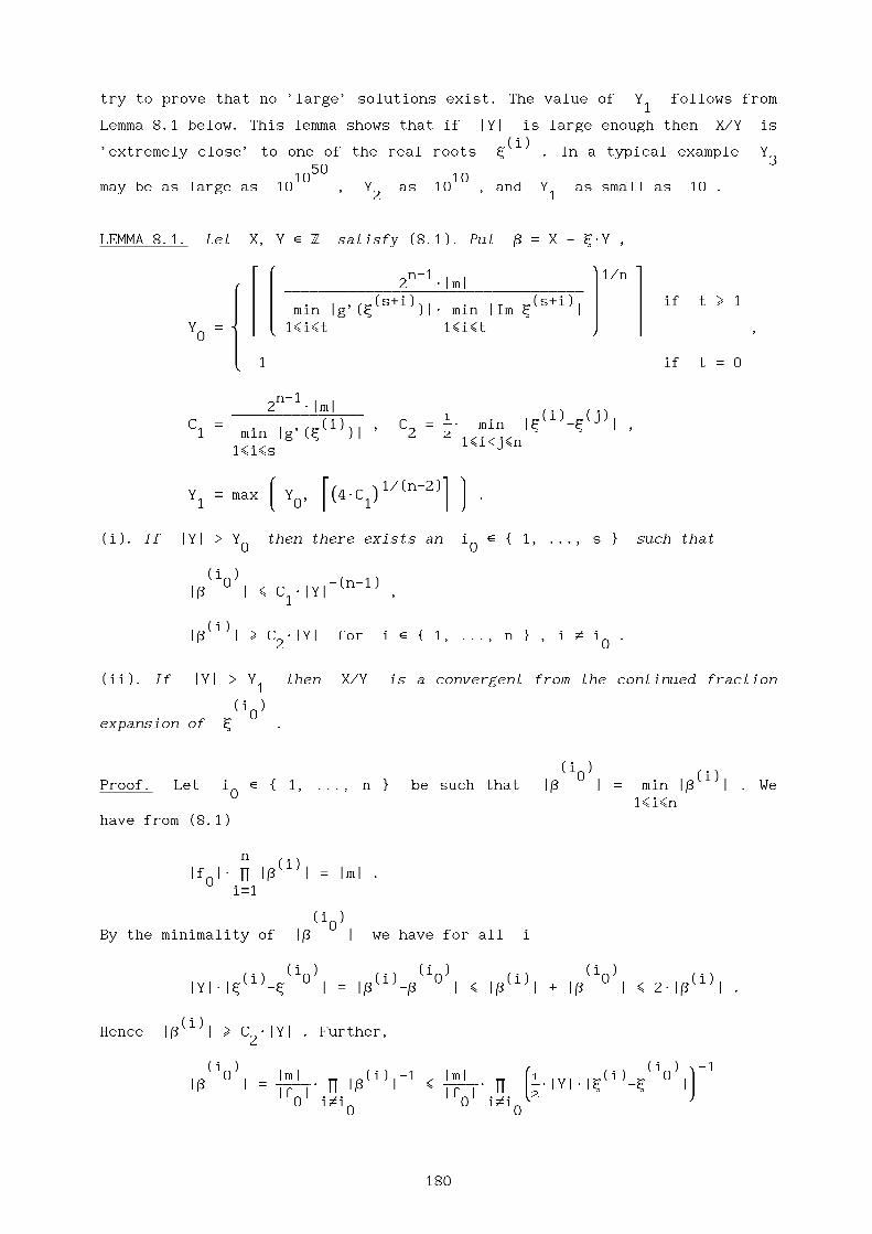
try to prove that no ’large’ solutions exist. The value of Y follows from1

Lemma 8.1 below. This lemma shows that if |Y| is large enough then X/Y is(i)

’extremely close’ to one of the real roots x . In a typical example Y3

5010 10

may be as large as 10 , Y as 10 , and Y as small as 10 .2 1

LEMMA_8.1. Let X, Y e Z satisfy (8.1). Put b = X - xWY ,

# & n-1 *1/n $2 W|m|

& | | -------------------------------------------------------------------------------------------------------------------------------------------------------------------------- | |(s+i) (s+i) if t > 1

| | | min |g’(x )|W min |Im x | | |Y = { | 7 1<i<t 1<i<t 8 | ,0

|7 1 if t = 0

n-12 W|m|

--------------------------------------------------------------------------- 1 (i) (j)C = (i) , C = -----W min |x -x | ,1 min |g’(x )| 2 2

1<i<j<n1<i<s

& #( )1/(n-2)$ *Y = max Y , 4WC .1 7 0 |9 10 | 8

(i). If |Y| > Y then there exists an i e { 1, ..., s } such that0 0

(i )0 -(n-1)

|b | < C W|Y| ,1

(i)|b | > C W|Y| for i e { 1, ..., n } , i $ i .

2 0

(ii). If |Y| > Y then X/Y is a convergent from the continued fraction1

(i )0

expansion of x .

(i )0 (i)

Proof. Let i e { 1, ..., n } be such that |b | = min |b | . We0

1<i<nhave from (8.1)

n(i)

|f |W p |b | = |m| .0

i=1

(i )0

By the minimality of |b | we have for all i

(i ) (i ) (i )(i) 0 (i) 0 (i) 0 (i)

|Y|W|x -x | = |b -b | < |b | + |b | < 2W|b | .

(i)Hence |b | > C W|Y| . Further,

2

(i ) (i ) -10 |m| (i) -1 |m| &1 (i) 0 *

|b | = --------------------W p |b | < --------------------W p -----W|Y|W|x -x ||f | |f | 72 80 i$i 0 i$i

0 0

180

n-1 n-12 W|m| 2 W|m|

= --------------------------------------------------------------------------------------------------------------------------------------- = ------------------------------------------------------------------------------------------ .(i ) (i )

| (i) 0 | n-1 | 0 | n-1|f W p (x -x )|W|Y| |g’(x )|W|Y|| 0 | | |

i$i0

Now, if i > s (and hence t > 1 ) then, by the definition of Y ,0 0

(i )(i ) 0 n-1

|X 0 | |b | 2 W|m||----- - x | = ----------------------------------- < ------------------------------------------------------- -n|Y | |Y| (i ) W|Y|

| 0 ||g’(x )|| |

Y n& 0 * (i)

< --------------- W min |Im x | ,7|Y|8

s+1<i<s+t

which is impossible if |Y| > Y . Hence i < s , and now (i) follows at0 0

once. Moreover, if |Y| > Y , then1

(i ) (i )|X 0 | 0 -1 -n 1 n-2 -n 1 -2|----- - x | = |b |W|Y| < C W|Y| < -----WY W|Y| < -----W|Y| ,|Y | 1 4 1 2

(i ) (i )X 0 1 -2 0

and thus | ----- - x | < -----W|Y| , since x is irrational. Now (ii)Y 2

follows from a well known result on continued fractions, cf. (3.6). p

Now let |Y| > Y and i e { 1, ..., s } as in Lemma 8.1. Choose1 0

j, k e { 1, ..., n } such that i , j, k are pairwise distinct and either0

--------------------(k) (j)

j, k e { 1, ..., s } or j + t = k (so that x = x ), but further the(i) (i)

choice of j, k is free. By b = X - YWx for i = i , j, k we get,0

on eliminating the X and Y ,

(i ) (i ) (i )0 ( (j) (k)) (j) ( (k) 0 ) (k) ( 0 (j))

b W x -x + b W x -x + b W x -x = 0 ,9 0 9 0 9 0

or, equivalently,

(i ) (i )0 (j) (k) (k) (j) 0

x -x b x -x b-------------------------------------------------- W -------------------- - 1 = - -------------------------------------------------- W ------------------------- . (8.2)(i ) (j) (i ) (j)0 (k) b (k) 0 b

x -x x -x

By Lemma 8.1, the right hand side of (8.2) is ’extremely small’. Put, if

j, k e {1, ..., s } (let us call it ’the real case’)

(i )| 0 (j) (k) || x -x b |

L = log | -------------------------------------------------- W -------------------- || (i ) (j) || 0 (k) b |x -x

and if j, k e { s+1, ..., s+2Wt } (let us call it ’the complex case’)

181

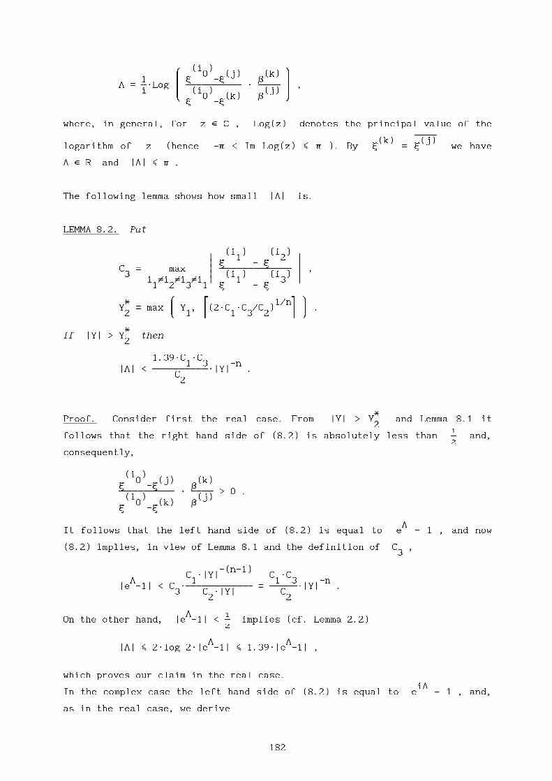
(i )& 0 (j) (k) *

1 x -x bL = -----WLog | -------------------------------------------------- W -------------------- | ,

i (i ) (j)7 0 (k) b 8x -x

where, in general, for z e C , Log(z) denotes the principal value of the--------------------

(k) (j)logarithm of z (hence -p < Im Log(z) < p ). By x = x we have

L e R and |L| < p .

The following lemma shows how small |L| is.

LEMMA_8.2. Put

(i ) (i )| 1 2 || x - x |

C = max | ----------------------------------------------------------------- | ,3 | (i ) (i ) |

i $i $i $i | 1 3 |1 2 3 1 x - x

* & # 1/n$ *Y = max Y , (2WC WC /C ) .2 7 1 | 1 3 2 | 8

*If |Y| > Y then

2

1.39WC WC1 3 -n

|L| < --------------------------------------------------W|Y| .C2

*Proof. Consider first the real case. From |Y| > Y and Lemma 8.1 it

21

follows that the right hand side of (8.2) is absolutely less than ----- and,2

consequently,

(i )0 (j) (k)

x -x b-------------------------------------------------- W -------------------- > 0 .(i ) (j)0 (k) b

x -x

LIt follows that the left hand side of (8.2) is equal to e - 1 , and now

(8.2) implies, in view of Lemma 8.1 and the definition of C ,3

-(n-1)C W|Y| C WC

L 1 1 3 -n|e -1| < C W------------------------------------------------------------ = -------------------------W|Y| .

3 C W|Y| C2 2

L 1On the other hand, |e -1| < ----- implies (cf. Lemma 2.2)

2

L L|L| < 2Wlog 2W|e -1| < 1.39W|e -1| ,

which proves our claim in the real case.iL

In the complex case the left hand side of (8.2) is equal to e - 1 , and,

as in the real case, we derive

182

C WCiL 1 3 -n 1|e -1| < -------------------------W|Y| < ----- .

C 22

iL 1Since |e -1| = 2W|sin L/2| , it follows that |sin L/2| < ----- , and therefore

4

by Lemma 2.3

1/4 1/4 iL iL|L| < 2W-----------------------------------W|sin L/2| = -----------------------------------W|e -1| < 1.02W|e -1| ,

sin 1/4 sin 1/4

which proves the lemma in the complex case. p

In the ring of integers of the field K (as well as in any other order R

of K ) there exists a system of fundamental units e , ..., e , where1 r

r = s + t - 1 (Dirichlet’s Unit Theorem). Note that since F is irreducible

and we have supposed s > 0 , the only roots of unity belonging to K are

+1 . We shall not discuss here the problem of finding such a system (forv

efficient methods see e.g. Berwick [1932], Billevic [1956], [1964], Pohst and

Zassenhaus [1982], Buchmann [1985], [1986]). We simply assume that a system

of fundamental units is known. On the other hand, there exist only finitely

many non-associates m , ..., m in K such that f WN(m ) = m for1 n 0 i

i = 1, ..., n (we use N(W) to denote the norm of the extension K/Q ). We

also assume that a complete set of such m ’s is known. Let M be the seti

of all zWm , where z is a root of unity in K . (In the important casei

|f | = |m| = 1 , it is clear that M = { -1, 1 } ). Then, for any integral0

solution (X,Y) of (8.1) there exist some m e M and a , ..., a e Z ,1 r

such that

a a1 r

b = mWe W...We .1 r

Thus, the initial problem of solving (8.1) is reduced to that of finding alla a1 r

integral r-tuples (a ,...,a ) such that mWe W...We for some m e M be1 r 1 r

of the special shape X - YWx , with X, Y e Z . As we have seen, X and Y

can be eliminated, so that we obtain (8.2). Thus the problem reduces to

solving finitely many equations of the type

( )a ( (i ))a(i ) (k) i (i ) 0 i0 (j) (k) r |e | (k) (j) 0 r |e |

x -x m i x -x m i--------------------------------------------------W--------------------W p |--------------------| - 1 = - --------------------------------------------------W-------------------------W p |-------------------------|(i ) (j) (j) (i ) (j) (j)0 (k) m i=17e 8 (k) 0 m i=17e 8

x -x i x -x i

(the so-called ’unit equation’). In the real case we have

183

(i ) (k)| 0 (j) (k) | r | e || x -x m | | i |

L = log | -------------------------------------------------- W -------------------- | + S a Wlog | -------------------- | , (8.3)| (i ) (j) | i | (j) || 0 (k) m | i=1 | e |x -x i

and in the complex case

(i ) (k)& 0 (j) (k) * r &e *x -x m i

L = Arg | -------------------------------------------------- W -------------------- | + S a WArg|--------------------| + a W2p , (8.4)(i ) (j) i (j) 0

7 0 (k) m 8 i=1 7e 8x -x i

with a e Z , and -p < Arg(z) < p for every z e C . Note that L in the0

real case, and iWL in the complex case, is a linear form in (principal)

logarithms of algebraic numbers, where the coefficients a are integers.i

The Gelfond-Baker theory provides an explicit lower bound for |L| in terms

of max|a | . Using this in combination with Lemma 8.2 we can find ani

explicit upper bound for max|a | . This is what we do in the next section.i

8.3. Upper bounds.

Let A = max |a | . First we find an upper bound for A in terms of |Y| .i

1<i<r

LEMMA_8.3. Let I = { h , ..., h } C { 1, ..., n } . Put1 r

(h )( i )

U = log|e | ,I 9 l 01<i<r,1<l<r

(where i indicates a row and l a column of the matrix),

r-1 -1U = (u ) , N[U ] = max S |u | .I il I il

1<i<r l=1

Put also

min (i) max (i)m = |m | , m = |m | ,- 1<i<n + 1<i<n

meM meM

(i ) (i )1 max 1 2----- + |x -x |2 1<i <i <n

1 2C = ---------------------------------------------------------------------------------------------------------------------------------- ,4 m

-

( -1 -1 )C = min (n-1)Wmin N[U ], max N[U ] .5 9 I I 0

I I

Then, for

184

( 1/n )|Y| > max Y , 2W|m| , m /C ,

9 1 + 2 0

we have

( )A < C Wlog C W|Y| .

5 9 4 0

a a1 r

Proof. By b = mWe W...We we have1 r

& (h ) (h ) *1 1

| log|b /m | | & a *1

| . | | . |. .

| . | = U W| . | . (8.5)I

| | | a |(h ) (h ) r

| r r | 9 0log|b /m |

7 8

On the other hand, for every h e { 1, ..., n } , using the end of the proof

of Lemma 8.1,

(i ) (i )(h) (h) 0 0 (h)

|b | = |X-YWx | < |X-YWx | + |Y|W|x -x |

(i )1 0 (h)

< ------------------------- + |Y|W|x -x |2W|Y|

(i ) (i )( 1 max 1 2 )

< ----- + |x -x | W|Y| ,9 2 1 1 . Indeed, by4

n(i) |m|

p |m | = -------------------- < |m||f |

i=1 0

(i) 1/n 1/nit follows that min |m | < |m| , hence m < |m| . Therefore

-1<i<n

(i ) (i )( 1 max 1 2 ) -1/n |Y|

C W|Y| > ----- + |x -x | W|Y|W|m| > ----------------------------------- > 1 .4 9 2 1 0 . (8.6)| (h)| 9 4 0 9 4 0|m |

185

Next we show that

| (i)|| |b || ( )|log|--------------------|| < (n-1)Wlog C W|Y| for i = 1, ..., n . (8.7)| | (i)|| 9 4 0

|m |

(i) (i)Indeed, in view of (8.6), a stronger inequality is true if |b /m | > 1 .

(i) (i)Suppose now that |b /m | < 1 . By

n | (h)||b |

p |--------------------| = 1| (h)|

h=1|m |

it follows that

n| (i)| | (i)| | (h)|

| |b || |b | S |b | ( )|log|--------------------|| = -log|--------------------| = log|--------------------| < (n-1)Wlog C W|Y| ,| | (i)|| | (i)| h=1 | (h)| 9 4 0

|m | |m | |m |h$i

in view of (8.6). Now the inequality

-1 ( )A < (n-1)Wmin N[U ]Wlog C W|Y|

I 9 4 0I

-1follows from (8.5), (8.7), the definition of N[U ] and the fact that, as

Iwe have not put so far any restriction on I , this could be chosen so that

-1N[U ] be minimal. It remains to show that

I

-1A < max N[U ]Wlog(C W|Y|) .

I 4I

Choose I such that i m I . Then, by Lemma 8.1, for every h e I ,0

(h) (h)|b /m | > C W|Y|/m > 1 and now, in view of (8.6),

2 +

| (h)|| |b || ( )|log|--------------------|| < log C W|Y| ,| | (h)|| 9 4 0

|m |

which implies our assertion. p

Lemmas 8.2 and 8.3 immediately yield

LEMMA_8.4. Put

n1.39WC WC WC

1 3 4 ( * 1/n )C = ----------------------------------------------------------------- , Y’ = max Y , 2W|m| , m /C .6 C 2 9 2 + 2 0

2

If |Y| > Y’ then2

(-n )|L| < C Wexp ----------WA .

6 9C 05

186

Next we apply Lemma 2.4 (Waldschmidt). It yields in the real case (assuming

that L $ 0 )

( )|L| > exp -C W(log A + C ) , (8.8)

9 7 8 0

and in the complex case this holds when A is replaced by A’ = max |a | .i

0<i<rThe precise values for C and C are given in Section 2.3. It should be

7 8noted that in the complex case a makes now its appearance, while it was

0not present in Lemmas 8.3 and 8.4. In order to obtain an upper bound for A ,

we must find an upper bound for A’ in terms of A . Indeed, using

Arg(z Wz ) = Arg(z ) + Arg(z ) + kW2p , k e { -1, 0, 1 } ,1 2 1 2

we find from (8.4) and the proof of lemma 8.2 that if A > 2 then

1 1|a | < ----- + -----WrWA + |L|/2p < 1 + rWA < rWA .0 2 2

Thus we may apply (8.8) in both cases with the same A if we replace C by8

C’ = C in the real case,8 8

C’ = C + log r in the complex case.8 8

We can now give an upper bound for A .

LEMMA_8.5. Put

2WC C WC5 ( 5 7 )

C = --------------------W log C + C WC’ + C Wlog ------------------------- .9 n 9 6 7 8 7 n 0

If |Y| > Y’ , then A < C .2 9

L 1Proof. As we have seen in the proof of Lemma 8.2, |e -1| < ----- in the real

2

(i )iL 1 0

case, and |e -1| < ----- in the complex case. Note that b $ 0 . Hence2

(8.2) implies L $ 0 . Therefore Lemma 8.4 and (8.8) yield

C5 ( )

A < ----------W log C + C WC’ + C Wlog A .n 9 6 7 8 7 0

The result now follows from Lemma 2.1. p

Remark. From this upper bound for A an upper bound for |Y| can be

derived, thus a value for Y (cf. Section 8.2). We shall not do this. Note3

that Y’ (cf. Lemma 8.4) is not necessarily equal to Y (cf. Section 8.2).2 2

187

8.4. Reducing the upper bound.

We are now left with a problem of the following type. Let be given real

numbers d, m , ..., m ( q > 2 , the case q = 1 is trivial). Write1 q

L = d + a Wm + ... + a Wm ,1 1 q q

where the a ’s belong to Z , and put A = max |a | . If K , K , K arei i 1 2 3

1<i<qq

given positive numbers, then find all q-tuples (a ,...,a ) e Z satisfying1 q

( )|L| < K Wexp -K WA , A < K . (8.9)

1 9 2 0 3

In our case, it follows from (8.3) or (8.4) how to define q, d and the

m ’s , and from Lemmas 8.4 and 8.5 how to define K , K , K . In general,i 1 2 3K and K are ’small’ constants, whereas K is ’very large’. Put1 2 3

L = a Wm + ... + a Wm ,0 1 1 q q

so that L = d + L . We apply the methods of Chapter 3 to problem (8.9).0

Below we distinguish three cases. In the first two we suppose that the m ’si

are Q-independent.

(i). Let d = 0 , so that L = L . Then the linear form is homogeneous, and0

we apply the method of Section 3.7.

(ii) Let d $ 0 . Then the linear form is inhomogeneous, and we apply the

method of Section 3.8.

(iii). Suppose now that the m ’s are Q-dependent. Let G be thei

approximation lattice for the linear form L , as defined in Section 3.7.

Then we expect the lower bound for |x| ( x e G , x $ 0 ) in general to be

’very small’, since the vector having as coordinates the coefficients of the

dependence relation will give rise to a very short vector in the lattice. So

the reduction process, as applied in the two previous cases, will not work.

In such a case we work as follows. Let M be a maximal subset of

{m ,...,m } consisting of Q-independent numbers. With an appropriate choice1 q

of subscripts we may assume that M = { m , ..., m } , p < q . Then we can1 p

find integers d > 0 and d for 1 < i < p < j < q such thatij

pdWm = S d Wm for j = p+1, ..., q .

j ij ii=1

(These numbers d, d can be found as coordinates of extremely shortij

vectors in reduced bases). On the other hand, (8.9) is equivalent to

188

( )|L’| < K’Wexp -K WA , A < K , (8.10)

1 9 2 0 3

where L’ = dWL and K’ = dWK . Now, with d’ = dWd and1 1

qa’ = dWa + S d Wai i ij j

j=p+1

we obtain

pL’ = d’ + S a’Wm .

i ii=1

( )Put D = max |d|, |d | : 1 < i < p < j < q . Then

9 ij 0

|a’| < (q-p+1)WDWA for i = 1, ..., p .i

Therefore, put A’ = max |a’| , then A’ < (q-p+1)WDWA , and (8.10) impliesi

1<i<p

( )|L’| < K’Wexp -K’WA’ , A’ < K’ , (8.11)

1 9 2 0 3

where

L’ = d’ + a’Wm’ + ... + a’Wm’ , K’ = dWK ,1 1 p p 1 1

K’ = K /(q-1+p)WD , K’ = (q-p+1)WK .2 2 3 3

Now, to solve (8.11) we apply the reduction process described in (i) or (ii),

depending on whether d’ = 0 or d’ $ 0 , and maybe more than once, if

necessary, until we find a very small upper bound for A’ . After having

found all solutions (a’,...,a’) of (8.11), we have a lower bound L > 01 p

for |L’| . It is reasonable to expect that L is not ’extremely small’,

because the integers a’, ..., a’ being ’small’ in absolute value cannot1 p

make |L’| ’extremely small’. Now combine |L’| > L with the first

inequality of (8.10) to get

K1 ( 1)

A < ----------Wlog ---------- .K 9L 02

Since L is not ’very small’, as argued heuristically, the above upper bound

for A is ’small’.

Returning now to the general case, we point out that if the reduced upper

bound for A (found after some reduction steps as described above) is not

small enough to admit enumeration of the remaining possibilities in a

189

reasonable time, then it might be necessary, or at least advisable, to use

the technique of Fincke and Pohst, cf. Section 3.6. However, when solving a

Thue equation, and not only an inequality for a linear form in logarithms, it

may be better to avoid this method, and to use continued fractions of the(i)

roots x . In practice we can search for the solutions (X,Y) of (8.1)

satisfying Y < |Y| < C as follows, referring to Lemma 8.1. Here e.g.1

C = Y , and we can imagine C here as being a ’large’ constant compared to2

Y , but not ’very large’ (cf. the introduction of Y , Y in Section 8.2).1 1 2

(i )~ 0

Let x be a rational approximation of x , such that

(i )|~ 0 | 1|x-x | < -------------------- . (8.12)

26WC

Since |Y| > Y , X/Y must be a convergent, p /q say, from the continued1 k k

(i )0

fraction expansion of x . Denote by a , a , a , ... the partial0 1 2

quotients in this expansion. First we claim that a > 3 . Indeed, by (3.5)k+1

(i ) p (i ) C1 1 | 0 k| | 0 X| 1

----------------------------------------------------------------- < ------------------------------------------------------- < |x - ----------| = |x - -----| < -------------------- .2 2 | q | | Y| n

(a +2)W|Y| (a +2)Wq k |Y|k+1 k+1 k

n-2If a = 1 or 2 , then we would have |Y| < 4WC , which is absurd,

k+1 11/(n-2)

since |Y| > Y > (4WC ) . Thus, a > 3 , and by (3.5) we have1 1 k+1

(i ) p 1 1| 0 k| ----------------------------------- --------------------.|x - ----------| < 2 < 2| q | a Wq 3Wq

k k+1 k k

Therefore,

p (i ) (i ) p|~ k| |~ 0 | | 0 k| 1 1 1|x - ----------| < |x-x | + |x - ----------| < -------------------- + -------------------- < --------------------| q | | | | q | 2 2 2

k k 6WC 3Wq 2Wqk k

and this means that p /q is in fact a convergent from the continuedk k

~fraction expansion of x too. Moreover, in view of the inequalities

(i ) p C C1 | 0 k| 1 1

------------------------------------------------------- < |x - ----------| < -------------------- < ------------------------- ,2 | q | n n

(a +2)Wq k |Y| |q |k+1 k k

a must be sufficiently large compared to q , namelyk+1 k

n-2|q |k

a > ----------------------------------- - 2 . (8.13)k+1 C

1

190

This inequality can be checked easily for all k such that q < C .k

(i )0

To sum up, we propose the following process for every real root x for

i = 1, ..., s (note that i is a priori not known). (1) Compute a0 0

(i )~ 0

rational approximation x of x satisfying (8.12) (a truncation of its~

decimal expansion will do). (2) Expand x into its continued fraction with

partial quotients a , a , a , ..., a and convergents p /q for all0 1 2 k+1 i i

i = 1, ..., k with q < C < q . (3) Test all these convergents for thek k+1

conditions (8.13) and F(p ,q ) = m . Concerning this last test, note that ifi i

nX/Y = p /q , then X = ZWp , Y = ZWq for some Z e Z with Z | m .

i i i iThis simple observation excludes in general most of the reducible quotients

X/Y , and all of them if m is an n-th-powerfree integer.

Having tested for all solutions in the range |Y| < C we may suppose that

|Y| > C . For such solutions (X,Y) we can obtain a lower bound for the

corresponding A as follows (the idea is due to A. Petho, cf. also Section 1b

of Blass, Glass, Meronk and Steiner [1987 ]). For every (i,j) e {1,...,r} *n

(j) ij{1,...,n} let v be the number +1 or -1 for which |e | > 1 ,

ij ir v

(j) ijand put E = p |e | . Then

j ii=1

r a(j) (j) (j) i A

|b | = |m |W p |e | < m WEi + j

i=1

and hence for any pair j , j with j $ j we have1 2 1 2

A A(j ) (j ) E + E

| 1 2 | j j|b -b | 1 2

|Y| = ----------------------------------------------------------------- < m W----------------------------------------------------------------- ,(j ) (j ) + (j ) (j )

| 1 2 | | 1 2 ||x -x | |x -x |

and from this we can find a lower bound for A , if we know that |Y| > C .

Of course, for an other pair j , j we may find a different lower bound,1 2

and therefore we can take the larger one.

8.5. An application: triangular numbers that are a product of three

consecutive numbers.

In this section we prove, as an application of the general theory described

in the previous sections, the following result. The problem was posed by S.P.

191

Mohanty (cf. Mohanty [1988]; the proof in this paper is incorrect). The n-th1

triangular number is for n e N defined as T = -----WnW(n+1) .n 2

THEOREM_8.6. The only triangular numbers that are a product of three

consecutive integers, are T = 1W2W3 , T = 4W5W6 , T = 5W6W7 ,3 15 20

T = 9W10W11 , T = 56W57W58 , T = 636W637W638 .44 608 22736

Proof. We have the diophantine equation nW(n+1) = 2WmW(m+1)W(m+2) in

n, m e N . Put x = 2Wm + 2 , y = 2Wn + 1 . Then we are lead to the equation2 3y = x - 4Wx + 1 in x, y e N , with x > 4 even and y > 3 odd. Theorem

8.7 below now completes the proof. p

THEOREM_8.7. The elliptic curve

2 3y = x - 4Wx + 1 (8.14)

has only the following 22 integral points:

(x,+y) = (-2,1), (-1,2), (0,1), (2,1), (3,4), (4,7), (10,31),

(12,41), (20,89), (114,1217), (1274,45473) .

We prove this theorem in two main steps. First, we reduce the problem to the

solution of two quartic Thue equations. Then we solve these equations using

the general theory developed in the previous sections.

Let L be the totally real field Q(j) , where

3j - 4Wj + 1 = 0 .

(1) (2)Let the conjugates of j be j = 0.254..., j = -2.114...,(3)j = 1.860... . From a table of Delone and Faddeev ([1964], p. 141) we see

that the class number of L is 1 , its ring of integers is Z[j] , its

discriminant is 229 , and a pair of independent units is j, 2 - j . From2 2

Table I of Buchmann [1986] we see that -7 + 2Wj , 2Wj + j is a pair of2 -1 2 -1

fundamental units in Z[j] . By -7 + 2Wj = -j W(2-j) , 2Wj + j = (2-j)

we see that j, 2 - j is also a pair of fundamental units in Z[j] .

The equation (8.14) of the elliptic curve can be written as

2 2 2y = ( x - j )W( x + xWj + (j -4) ) (8.15)

192

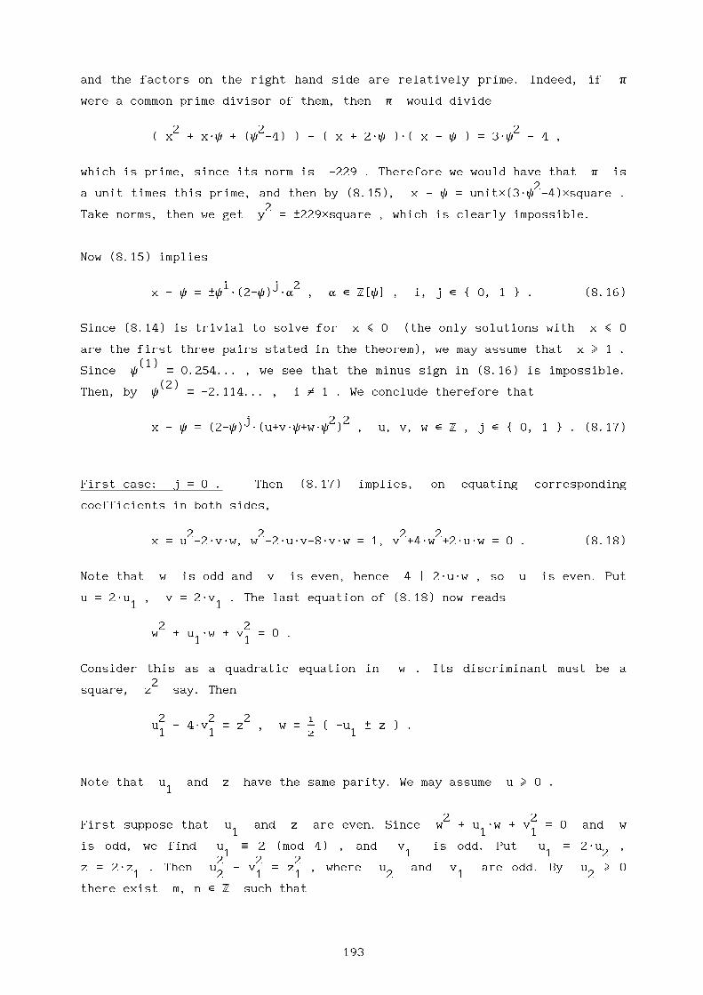
and the factors on the right hand side are relatively prime. Indeed, if p

were a common prime divisor of them, then p would divide

2 2 2( x + xWj + (j -4) ) - ( x + 2Wj )W( x - j ) = 3Wj - 4 ,

which is prime, since its norm is -229 . Therefore we would have that p is2

a unit times this prime, and then by (8.15), x - j = unit*(3Wj -4)*square .2

Take norms, then we get y = +229*square , which is clearly impossible.

Now (8.15) implies

i j 2x - j = +j W(2-j) Wa , a e Z[j] , i, j e { 0, 1 } . (8.16)

Since (8.14) is trivial to solve for x < 0 (the only solutions with x < 0

are the first three pairs stated in the theorem), we may assume that x > 1 .(1)

Since j = 0.254... , we see that the minus sign in (8.16) is impossible.(2)

Then, by j = -2.114... , i $ 1 . We conclude therefore that

j 2 2x - j = (2-j) W(u+vWj+wWj ) , u, v, w e Z , j e { 0, 1 } . (8.17)

First_case:__j_=_0_. Then (8.17) implies, on equating corresponding

coefficients in both sides,

2 2 2 2x = u -2WvWw, w -2WuWv-8WvWw = 1, v +4Ww +2WuWw = 0 . (8.18)

Note that w is odd and v is even, hence 4 | 2WuWw , so u is even. Put

u = 2Wu , v = 2Wv . The last equation of (8.18) now reads1 1

2 2w + u Ww + v = 0 .

1 1

Consider this as a quadratic equation in w . Its discriminant must be a2

square, z say. Then

2 2 2 1u - 4Wv = z , w = ----- ( -u + z ) .1 1 2 1

Note that u and z have the same parity. We may assume u > 0 .1

2 2First suppose that u and z are even. Since w + u Ww + v = 0 and w

1 1 1is odd, we find u _ 2 (mod 4) , and v is odd. Put u = 2Wu ,

1 1 1 22 2 2

z = 2Wz . Then u - v = z , where u and v are odd. By u > 01 2 1 1 2 1 2

there exist m, n e Z such that

193

2 2 2 2u = m + n , v = m - n , z = 2WmWn .2 1 1

It follows that

2 2 2 2 2u = 4W(m +n ) , v = 2W(m -n ) , w = -(m+n) .

Since the sign of z , and thus that of n , is of no importance, we may2

assume w = -(m+n) . After substitution in the second equation of (8.18) we

obtain the Thue equation

4 3 2 2 3 4m + 36Wm Wn + 6Wm Wn - 28WmWn + n = 1 .

The left hand side can be factored as

3 2 2 3( m + n )W( m + 35Wm Wn - 29WmWn + n ) ,

and therefore it can be solved very easily. Its only solutions are

+(m,n) = (1,0), (0,1) . They lead to +(u,v,w) = (4,2,-1), (4,-2,-1) , and

then by (8.18) we find x = 20, 12 respectively, which furnish the solutions

(x,+y) = (20,89), (12,41) for (8.14).

Secondly, we suppose that u and z are odd. Then v is even, so by1 1

u > 0 there exist m, n e Z with1

2 2 2 2u = m + n , 2Wv = 2WmWn , z = m - n .1 1

It follows that

2 2 2 2u = 2W(m +n ) , v = 2WmWn , w = -m or w = -n .

2We may assume that w = -m . Substituting this in the second equation of

(8.18) we find the Thue equation

4 3 3m + 8Wm Wn - 8WmWn = 1 .

The left hand side is again reducible. The only solutions, as is easily seen,

are +(m,n) = (1,0), (1,1), (1,-1) . Since m and n cannot have the same

parity, only the first pair is accepted. It leads to (u,v,w) = (2,0,-1) ,

and hence to (x,+y) = (4,7) for (8.14).

Second_case:__j_=_1_. Then, equating the coefficients in (8.17) we get

2 2 2x = 2Wu + v + 4Ww + 2WuWw - 4WvWw , (8.19)

194

2 2 2& u + 4Wv + 18Ww - 4WuWv + 8WuWw - 18WvWw = 1 ,{ (8.20)

2 27 2Wv + 9Ww - 2WuWv + 4WuWw - 8WvWw = 0 .

The first relation of (8.20) can be replaced by

2u - 2WvWw = 1 . (8.21)

Note that u is odd. Put z = v - 2Ww . Then the second equation of (8.20)

yields

2w = 2WzW(u-z) .

First we suppose that z is odd. Then there exist m, n e Z such that

2 2z = m , u - z = 2Wn ,

where we use that u > 0 and (u,w) = 1 . Thus, choosing signs properly,

2 2 2u = m + 2Wn , v = m + 4WmWn , w = 2WmWn .

Substituting this in (8.21) we obtain the Thue equation

4 3 2 2 4m - 4Wm Wn - 12Wm Wn + 4Wn = 1 . (8.22)

In Theorem 8.8(i) below we prove that this equation has only the solutions

+(m,n) = (1,0) , leading to (u,v,w) = (1,1,0) , and finally for (8.14) to

(x,+y) = (3,4) .

Secondly we suppose that z is even. Then there exist m, n e Z with

2 2z = 2Wm , u - z = n .

Thus, choosing signs properly, we find

2 2 2u = 2Wm + n , v = 2Wm + 4WmWn , w = 2WmWn .

Now, substituting into (8.21), we obtain the Thue equation

4 2 2 3 4n - 12Wn Wm - 8WnWm + 4Wm = 1 . (8.23)

In Theorem 8.8(ii) below we prove that this equation has only the solutions

+(m,n) = (0,1), (1,-1), (3,1), (-1,3) . They lead respectively to

(u,v,w) = (1,0,0), (3,-2,-2), (19,30,6), (11,-10,-6) , which lead for (8.14)

195

to the solutions (x,+y) = (2,1), (10,31), (1274,45473), (114,1217) . Thus

this result completes the proof of Theorem 8.7, provided the Thue equations

(8.22), (8.23) have as their only solutions the pairs (m,n) mentioned

above. We now proceed to prove this.

THEOREM_8.8. (i). The Thue equation

4 3 2 2 4X - 4WX WY - 12WX WY + 4WY = 1 (8.24)

has only the solutions +(X,Y) = (1,0) .

(ii). The Thue equation

4 2 2 3 4X - 12WX WY - 8WXWY + 4WY = 1 (8.25)

has only the solutions +(X,Y) = (1,0), (1,-1), (1,3), (3,-1) .

Proof. We use the notation and results of Sections 8.2 and 8.3. Let the

algebraic numbers y and v be defined by

4 2 4 3 2y - 12Wy - 8Wy + 4 = 0 , v - 4Wv - 12Wv + 4 = 0 .

Since v = 2/y , it follows that y and v generate the same field K over

Q . In the notation of Section 8.2 we have n = 4, s = 4, t = 0 , and x = y

or x = v . Simple computations show that for x = y, v we can take

Y = 1 , C = 0.843 , C = 0.589 , Y = 2, C = 6.645 ,0 1 2 1 3

*Y = 3 , m = m = 1 , C = 8.3374 .2 - + 4

In these computations we estimated C , C , C from above and C from1 3 4 2

below, using the following approximations for the conjugates of y and v :

(1) (1)y = -1.080 286 352 , v = -1.851 360 980 ,

(2) (2)y = 3.722 935 260 , v = 0.537 210 524 ,

(3) (3)y = 0.334 111 716 , v = 5.986 021 747 ,

(4) (4)y = -2.976 760 624 , v = -0.671 871 290 .

1 2 1 3Now we work in the order R of K with Z-basis { 1, y, -----Wy , -----Wy }

2 21 2

(note that -----Wy is an algebraic integer). Note that2

2 1 3v = ----- = 4 + 6Wy - -----Wy e R .

y 2

On the other hand, (8.24) and (8.25) are respectively equivalent to

196

Norm (X-YWy) = 1 and Norm (X-YWv) = 1 , which means that if (X,Y) isK/Q K/Q

a solution of (8.24) or (8.25), then X - YWy or X - YWv , respectively, is

a unit of the order R . A system of fundamental units of R is given by

1 2e = 1 + y , e = 3 + y , e = -----Wy .1 2 3 2

We do not prove this fact here. For a proof, see Tzanakis and de Wegera

[1989 ], Section III.2 and Appendix I.

Thus the solution of (8.24) and (8.25) is reduced to finding alla a a

3 1 2 3(a ,a ,a ) e Z such that the unit +e We We has the special shape

1 2 3 1 2 3X - YQy or X - YWv , respectively. In the notation of Lemma 8.3 we have,

after some numerical computations, that we leave to the reader to check, that

-1 -1min N[U ] = 0.634950... , max N[U ] = 1.210070... ,

I II I

(here, of course, I = { 1, 2, 3, 4 } ). Therefore we can take in Lemma 8.4

C = 1.211 .5

Also,

4C = 6.38771*10 , Y’ = 3 .6 2

(The values of C and C are estimated from above.)5 6

Now, relation (8.3) becomes in our case

(i ) (k)| 0 (j)| 3 |e ||x -x | | i |

L = log|--------------------------------------------------| + S a Wlog|--------------------| , (8.26)| (i ) | i | (j)|| 0 (k)| i=1 |e ||x -x | i

where x = y or v . As mentioned in Section 8.2, once i is fixed, we can0

choose j, k arbitrarily. Thus we can choose

& j = 3, k = 4 if i = 1 or 2 ,0

{ (8.27)7 j = 1, k = 2 if i = 3 or 4 .

0

Therefore, for each x e { y, v } we have four possibilities for L . For

each of these eight cases we have, as will be shown below,

38C = 5.71*10 , C = 6.17 ,7 8

and therefore, by Lemma 8.5, if |Y| > 3 , then for A = max |a | we havei

1<i<3

197

40the upper bound C = 3.26*10 . As is easily checked, the only solutions of

9either (8.24) or (8.25) with |Y| < 3 are those listed in the statement of

the theorem. Therefore we may assume that |Y| > 3 , so that

40A < 3.26*10 .

Before we apply the reduction method of Section 3.8 we show that the

application of Lemma 2.4 yields the above constants C , C . We apply this7 8

result in the case of L given by (8.26). In this case, we compute the V ’si

(k) (j)for the various a ’s appearing in L , as follows. If a = |e /e |

i i i ifor i = 1, 2, 3 , then a is a unit and hence a (appearing in the

i 0computation of h(a ) ) is equal to 1. Clearly, every conjugate of a is in

i iabsolute value less than

max (h)|e |

1<h<4 iH = ------------------------------------------------------- ,i min (h)

|e |1<h<4 i

and H > 1 . Therefore, h(a ) < H , and we can takei i i

( (k) (j) )V = max log H , |log|e /e || .i 9 i i i 0

(k) (j)Since the latter term equals the logarithm of either |e /e | or its

i iinverse, it follows that

V = log H .i i

(i ) (i )0 (j) 0 (k)

If a = |x -x |/|x -x | , then all conjugates of a are ini i

absolute value less than C . Therefore, h(a ) < (log a )/d + log C ,3 i 0 3

where a and d are as in the definition of h(a) for a = a . An upper0 i

bound for a can be computed as follows. Consider the algebraic numbers0

1 (i) (h)c = -----W(x -x ) for i, h e { 1, ..., 4 } with i $ h . It can beih 2

checked that the numbers c are algebraic integers for x = y or v .ih

Now, for each permutation s = (s s s s ) e S we consider the number1 2 3 4 4

c(s) = c /c (independent of s ), and the polynomials s s s 41 2 1 3

( )P(X) = p X - c(s) .

9 0seS

4

Consider also the number

D = p c .ih

1<i<h<4

198

Note that

2 1 2 1D = ---------------W p (x -x ) = ---------------WD ,

12 i h 122 1<i<h<4 2

where D is the discriminant of the defining polynomial of x , and2

therefore D = 229 . On the other hand, the coefficients of P(X) are up to

the sign the elementary symmetric functions of c(s) for s e S , and so4

(i)they are symmetrical expressions of the x ’s with rational coefficients.

This means that P(X) e Q[X] . On the other hand, by the definition of D ,4

any coefficient of P(X) multiplied by D is a polynomial of the c ’sih

with coefficients in Z and therefore it is an algebraic integer. Combine2

this with the fact that P(X) e Q[X] to see that 229 WP(X) e Z[X] . Hence,

since a is a root of P(X) , its leading coefficient a is at mosti 0

2229 . To conclude, we have h(a ) < 2W(log 229)/d + log C and it is clear

i 3that |log a |/d < log C . Since a m Q we have d > 2 , so we can take

i 3 i

V = log 229 + log C .i 3

Simple computations now show that

log H = 4.074586... , log H = 5.667432... ,1 2

log H = 4.821584... ,3

log C = 1.262065... if x = y ,3

log C = 1.893823... if x = v ,3

log 229 + log C < 7.327545... .3

Therefore we apply Lemma 2.4 (Waldschmidt) with n = 4, D < 24, e(n) = 73,

(k) (k) (k) (i )|e | |e | |e | | 0 (j)|| 1 | | 3 | | 2 | |x -x |

a = |--------------------| , a = |--------------------| , a = |--------------------| , a = |--------------------------------------------------| ,1 | (j)| 2 | (j)| 3 | (j)| 4 | (i ) |

|e | |e | |e | | 0 (k)|1 3 2 x -x

for x = y or v , and b = a , b = a , b = a , b = 1 , B = A ,1 1 2 3 3 2 4

+ +V = log H , V = log H , V = V = log H , V = V = log 229 + log C .1 1 2 3 3 3 2 4 4 3Thus we find that

( )|L| > exp -C W(log A + C ) ,

9 7 8 0

38with C = 5.71*10 and C = 6.17 .

7 8

199

We have now to apply the reduction process described in Section 3.7. In our

situation we have to solve (8.9) with

4 n 4 40K = C = 6.38771*10 , K = ---------- = ------------------------- > 3.303 , K = 3.26*101 6 2 C 1.211 3

5

( K is estimated from below), and2

L = d + a Wm + a Wm + a Wm ,1 1 2 2 3 3

where for d and the m ’s we have, in view of (8.26) and (8.27):i

| (1) (3)| | (2) (3)|& |x -x | |x -x |d = d := log|---------------------------------------------| or d = d := log|---------------------------------------------| ,

| 1 | (1) (4)| 2 | (2) (4)||x -x | |x -x |

|{ where x = y or v , (8.28)

(4)| |e |

| i || m = log|--------------------| , for i = 1, 2, 3 ,

i | (3)|7 |e |

i

or

| (3) (1)| | (4) (1)|& |x -x | |x -x |d = d := log|---------------------------------------------| or d = d := log|---------------------------------------------| ,

| 3 | (3) (2)| 4 | (4) (2)||x -x | |x -x |

|{ where x = y or v , (8.29)

(2)| |e |

| i || m = log|--------------------| , for i = 1, 2, 3 .

i | (1)|7 |e |

i

Numerical details are given in the preprint version of Tzanakis and de Wegera 140

[1989 ] (to be obtained from the author). We take c = 10 , and we work0

with the lattice with associated matrix

& *1 0 0

| |A = | 0 1 0 | .

| |[c Wm ] [c Wm ] [c Wm ]

7 0 1 0 2 0 3 8

Note that in each of the four cases of (8.28) (resp. (8.29)) we have the same

lattice, G (resp. G ), say. In each case d $ 0 , and we had no1 2

numerical evidence that the m ’s are Q-dependent. Therefore we worked as ini

case (ii) of Section 8.4.

3For each G we have applied the integral version of the L -algorithm, and

i-1

each time we have computed the integral 3*3-matrices B, U, U , as defined

in Section 3.7. In our cases, the coordinates of the vectors of the reduced

bases (i.e. the elements of B ) turned out to have 46 to 48 digits, i.e. the1/3

lengths of the reduced basis vectors are of the size of c , as expected.0

200

In each of the eight cases we computed the coordinates s , s , s of1 2 3

& 0 *| |

x = 0| |7-[c Wd]8

0

with respect to the reduced basis b , b , b of the lattice. From our1 2 3

computations we found

46|b | > 3.247*10 in the case of lattice G ,1 1


Ns N > 0.029 in all 8 cases.3

This means that in view of Lemma 3.5, in all cases i = 3 , and0

1 46 44l(G ,x) > 0.029W-----W3.247*10 > 4.708*10 .

i 2

Then the assumptions of Lemma 3.10 are fulfilled with n = 3, g = 1, C = c ,0

40c = K , d = K , X = X = K , since r27WK < 1.112*10 , which implies

1 2 0 1 3 3

1 ( 140 4 40)A < -------------------------Wlog 10 W6.38771*10 /3.26*10 < 72.8 .

3.303 9 0

It follows that A < 72. We repeat the procedure with K = 72 and3

12c = 10 . We found from our computations0



Ns N > 0.143 in all 8 cases.3

This means that in view of Lemma 3.5, in all cases i = 3 , and0

1 4 2l(G ,x) > 0.143W-----W1.092*10 > 7.807*10 .

i 2

2Then the assumptions of Lemma 3.10 are fulfilled, since r27WK < 3.742*10 ,

3which implies

1 ( 12 4 )A < -------------------------Wlog 10 W6.38771*10 /72 < 10.5 .

3.303 9 0

It follows that A < 10 . We enumerated all remaining possibilities, and

found no other solutions of (8.24) and (8.25) than those mentioned. p

The computations for the proof of Theorem 8.8 took 35 sec.

201

8.6. The Thue-Mahler equation, an outline.

Let F(X,Y) be as in Section 8.1. Let p , ..., p be fixed distinct prime1 s

numbers. The diophantine equation

s ni

F(X,Y) = + P pi

i=1

in the variables X, Y e Z , n , ..., n e N , with (X,Y) = 1 , is known1 s 0

as a Thue-Mahler equation. It was proved by Mahler [1933] that this equation

has only finitely many solutions, and by Coates [1970] that they can, at

least in principle, be determined effectively, since an effectively

computable upper bound for the variables can be derived from the p-adic

theory of linear forms in logarithms. For the history of this equation we

refer to Shorey and Tijdeman [1986], Chapter 7.

We believe that it is possible to solve Thue-Mahler equations, not only in

principle, but in practice. This can be done by reducing the above mentioned

upper bounds, using a combination of real and p-adic computational3

diophantine approximation techniques, based on the L -algorithm for reducing

bases of lattices (cf. Sections 3.7 and 3.8 for the real case, 3.11 and 3.12

for the p-adic case, Section 1.5 for a short outline of how to combine the

real and p-adic techniques, and Sections 4.8 and 6.4 for some explicit

examples of such combined techniques). The method can be considered as a

p-adic analogue of the method for solving Thue equations, on which we

reported in the preceding sections.

3Such an idea (but without using the L -algorithm) was used by Agrawal,

Coates, Hunt and van der Poorten [1980], who solved the equation

3 2 2 3 nX - X WY + XWY + Y = +11 .

This is to the author’s knowledge the only example in the literature where a

Thue-Mahler equation has been solved by the Gelfond-Baker method. Other

methods may apply as well for solving Thue-Mahler equations. For example,

3 3 nX + 3WY = 2 ,

has been solved by Tzanakis [1984] by a different method. The advantage of

the Gelfond-Baker method above many other ideas is that it works in principle

for any Thue-Mahler equation, because it is not very much dependent on the

parameters of the particular equation that one wants to solve.

202

Both examples of Thue-Mahler equations mentioned above are of the simplest

kind, in view of the fact that the cubic field Q(y) , where y is a root of

F(x,1) = 0 , has only one fundamental unit, and there occurs only one prime.

Therefore it is sufficient to use two-dimensional real continued fractions

and one-dimensional p-adic continued fractions, instead of the more3

complicated L -algorithm (which anyway was not yet available in 1980, when

Agrawal, Coates, Hunt and van der Poorten did their work). With the use of3

the L -algorithm the method can in principle be extended to the general

situation, where there are more than one fundamental units, and more than one

primes. In a forthcoming publication, Tzanakis and the present author plan tob

give details and worked-out examples (Tzanakis and de Weger [1989 ]).

203

References.

After each reference we mention in brackets the section(s) in which the

reference occurs.

Agrawal, M.K., Coates, J.H., Hunt, D.C. and van der Poorten, A.J. [1980],

Elliptic curves of conductor 11, Math. Comp. 35, 991-1002. (3.8;3.10;

8.6)

Alex, L.J. [1976], Diophantine equations related to finite groups, Comm.

Algebra 4, 77-100. (6.1;6.5)

a a b c d e fAlex, L.J. [1985 ], On the diophantine equation 1 + 2 = 3 5 + 2 3 5 ,

Math. Comp. 44, 267-278. (1.1;5.4)

b a b c d e fAlex, L.J. [1985 ], On the diophantine equation 1 + 2 = 3 7 + 2 3 7 ,

Arch. Math. 45, 538-545. (1.1;5.4)

Babai, L. [1986], On Lovssz lattice reduction and the nearest lattice point

problem, Combinatorica 6, 1-13. (1.4;3.4)

Bachman, G. [1964], Introduction to p-adic Numbers and Valuation Theory,

Academic Press, New York and London. (2.3)

Baker, A. [1966], Linear forms in the logarithms of algebraic numbers,

Mathematika 13, 204-216. (2.4)

Baker, A. [1968], Contributions to the theory of diophantine equations, I,

On the representation of integers by binary forms, II, The diophantine

2 3equation y = x + k , Phil. Trans. R. Soc. London, A 263, 173-208.

(8.1)

Baker, A. [1972], A sharpening of the bounds for linear forms in logarithms

I, Acta Arith. 21, 117-129. (1.2)

Baker, A. [1977], The theory of linear forms in logarithms, Transcendence

Theory: Advances and Applications, A. Baker (ed.), Academic Press,

London, pp. 1-27. (2.4)

2 2Baker, A. and Davenport, H. [1969], The equations 3x - 2 = y and

2 28x - 7 = z , Q. Jl. Math. Oxford (2) 20, 129-137. (1.1;1.4;3.3)

Berwick, W.E.H. [1932], Algebraic number fields with two independent units,

Proc. London Math. Soc. 34, 360-378. (8.2)

Beukers, F. [1981], On the generalized Ramanujan-Nagell equation, Acta Arith.

I: 38, 389-410; II: 39, 113-123. (1.1;4.1)

205

vBillevic, K.K. [1956], On the units of algebraic fields of third and fourth

degree (Russian), Mat. Sbornik Vol. 40, 82, 123-137. (8.2)

vBillevic, K.K. [1964], A theorem on the units of algebraic fields of n-th

degree (Russian), Mat. Sbornik Vol. 64, 106, 145-152. (8.2)

aBlass, J., Glass, A.M.W., Meronk, D.B. and Steiner, R.P. [1987 ], Practical

solutions to Thue equations of degree 4 over the rational integers,

Preprint, Bowling Green State University. (3.8;8.1)

bBlass, J., Glass, A.M.W., Meronk, D.B. and Steiner, R.P. [1987 ], Practical

solutions to Thue equations over the rational integers, Preprint,

Bowling Green State University. (3.8;8.1;8.4)

Blass, J., Glass, A.M.W., Manski, D.K., Meronk, D.B. and Steiner, R.P.

a[1988 ], Constants for lower bounds for linear forms in the logarithms

of algebraic numbers I: The general case, Preprint, Bowling Green State

University. (2.4)

Blass, J., Glass, A.M.W., Manski, D.K., Meronk, D.B. and Steiner, R.P.

b[1988 ], Constants for lower bounds for linear forms in the logarithms

of algebraic numbers II: The homogeneous rational case, Preprint,

Bowling Green State University. (2.4)

Borevich, Z.I. and Shafarevich, I.R. [1966], Number Theory, Academic Press,

New York. (2.1;7.3)

Bremner, A., Calderbank, R., Hanlon, P., Morton, P. and Wolfskill, J. [1983],

2 a

Two-weight ternary codes and the equation y = 4*3 + 13 , J. Number

Theory 16, 212-234. (4.1)

Brenner, J.L. and Foster, L.L. [1982], Exponential diophantine equations,

Pacific J. Math. 101, 263-301. (6.1)

Brent, R.P. [1978], A Fortran multiple-precision arithmetic package, ACM

Trans. Math. Software 4, 57-70; and: Algorithm 524. MP, a Fortran

multiple-precision arithmetic package, ACM Trans. Math. Software 4,

71-81. (2.5)

Brentjes, A.J. [1981], Multi-dimensional Continued Fraction Algorithms,

MC Tract 145, Centr. Math. Comput. Sci., Amsterdam. (1.3;3.4)

Brown, E. [1985], Sets in which xy + k is always a square, Math. Comp. 45,

613-620. (1.1)

Buchmann, J. [1985], The generalized Voronoi-algorithm in totally real

algebraic number fields, Proceedings EUROCAL ’85, Linz, Austria, Vol. 2,

Lecture Notes in Comput. Sci. 204, Springer Verlag, Berlin, pp. 479-486.

(8.2)

Buchmann, J. [1986], A generalization of Voronoi’s unit algorithm I & II, J.

Number Theory 20, 177-191 & 192-209. (8.2;8.5)

206

Cassels, J.W.S. [1957], An Introduction to Diophantine Approximation,

Cambridge University Press, Cambridge. (1.3)

Cherubini, J.M. and Walliser, R.V. [1987], On the computation of all

imaginary quadratic fields of class number one, Math. Comp. 49, 295-300.

(3.2)

Coates, J. [1969], An effective p-adic analogue of a theorem of Thue, Acta

Arith. 15, 279-305. (2.4;6.1)

Coates, J. [1970], An effective p-adic analogue of a theorem of Thue II: The

greatest prime factor of a binary form, Acta Arith. 16, 399-412. (2.4;

6.1;8.6)

Delone, B.N. and Faddeev, D.K. [1964], The theory of irrationalities of the

third degree, Transl. of Math. Monogr., Vol 10, A.M.S., Providence R.I.

(8.5)

aEllison, W.J. [1971 ], Recipes for solving diophantine problems by Baker’s

method, Swm. Thworie des Nombres, Universitw de Bordeaux I, 1970-1, Lab.

Th. Nombr. C.N.R.S., Exp. 11, 10 pp. (1.4;3.8)

bEllison, W.J. [1971 ], On a theorem of S. Sivasankaranarayana Pillai, Swm.

Thworie des Nombres, Universitw de Bordeaux I, 1970-1, Lab. Th. Nombr.

C.N.R.S., Exp. 12, 10 pp. (3.2;5.1)

Ellison, W.J., Ellison, F., Pesek, J., Stahl, C.E. and Stall, D.S. [1972],

2 3The diophantine equation y + k = x , J. Number Theory 4, 107-117.

(3.3;8.1)

Evertse, J.-H. [1983], Upper Bounds for the Numbers of Solutions of

Diophantine Equations, MC Tract 168, Centr. Math. Comput. Sci.,

Amsterdam. (1.1)

Evertse, J.-H., Gyory, K., Stewart, C.L. and Tijdeman, R. [1988], S-unit

equations and their applications, New advances in transcendence theory

(Proc. Symp. Durham July 1986), A. Baker (ed.), Cambridge University

Press, Cambridge, pp. 110-174. (1.1)

Faltings, G. [1983], Endlichkeitssatze ftr abelsche Varietaten tber

Zahlkorpern, Invent. Math. 73, 349-366. (1.1)

Fincke, U. and Pohst, M. [1985], Improved methods for calculating vectors of

short length in a lattice, including a complexity analysis, Math. Comp.

44, 463-471. (3.6)

Gasl, I. [1988], On the resolution of inhomogeneous norm form equations in

two dominating variables, Math. Comp. 51, 359-373. (3.3)

Grinstead, C.M. [1978], On a method of solving a class of diophantine

equations, Math. Comp. 32, 936-940. (1.1)

207

Grosswald, E. [1984], Topics from the Theory of Numbers, 2nd. ed.,

Birkhauser, Boston. (1.1)

Hardy, G.H. and Wright, E.M. [1979], An Introduction to the Theory of

Numbers, (5th ed.), Oxford University Press, Oxford. (1.3;3.2)

Hasse, H. [1966], Tber eine diophantische Gleichung von Ramanujan-Nagell und

ihre Verallgemeinerung, Nagoya Math. J. 27, 77-102. (4.1)

Hunt, D.C. and van der Poorten, A.J., Solving diophantine equations

2 ux + d = a , unpublished. (3.2;4.1)

Kiss, P. [1979], Zero terms in second order linear recurrences, Math. Sem.

Notes Kobe Univ. (Japan) 7, 145-152. (4.3)

Knuth, D.E. [1981], The Art of Computer Programming, Vol. 2: Seminumerical

Algorithms, (2nd ed.), Addison-Wesley, Reading Mass. (2.5)

Koblitz, N. [1977], p-adic Numbers, p-adic Analysis, and Zeta-functions,

Springer Verlag, New York. (2.3)

Koblitz, N. [1980], p-adic Analysis: a Short Course on Recent Work, Cambridge

University Press, Cambridge. (2.3)

Koksma, J.F. [1937], Diophantische Approximationen, Ergebnisse der Mathematik

und ihrer Grenzgebiete, Vol. 4, Springer Verlag, pp. 407-571. (1.3)

Lagarias, J.C. and Odlyzko, A.M. [1985], Solving low-density subset sum

problems, J. Assoc. Comput. Mach. 32, 229-246. (3.4)

Langevin, M. [1976], Quelques applications de nouveaux rwsultats de van der

Poorten, Swm. Delange-Pisot-Poitou 1975/76, Paris, Exp. G12, 11 pp.

(1.1)

Lehmer, D.H. [1964], On a problem of Stormer, Illinois J. Math. 8, 57-79.

(4.9;5.1)

Lenstra, A.K. [1984], Polynomial-time Algorithms for the Factorization of

Polynomials, Dissertation, University of Amsterdam. (1.4;3.4;3.5)

LLL = Lenstra, A.K., Lenstra, H.W. Jr. and Lovssz, L. [1982], Factoring

polynomials with rational coefficients, Math. Ann. 261, 515-534. (1.4;

3.4;3.5)

Loxton, J.H., Mignotte, M., van der Poorten, A.J. and Waldschmidt, M. [1987],

A lower bound for linear forms in the logarithms of algebraic numbers,

C.R. Math. rep. Acad. Sci. Canada 11, 119-124. (2.4)

Lutz, W. [1951], Sur les approximations diophantiennes linwaires P-adiques,

Thrse, Universitw de Strasbourg. (1.3)

MacWilliams, F.J. and Sloane, N.J.A. [1977], The Theory of Error-Correcting

Codes, North-Holland, Amsterdam. (4.1)

Mahler, K. [1933], Zur Approximation algebraischer Zahlen I: Tber den

grossten Primteiler binarer Formen, Math. Ann. 107, 691-730. (6.1;8.6)

208

Mahler, K. [1934], Eine arithmetische Eigenschaft der rekurrierenden Reihen,

Mathematika B (Leiden) 3, 153-156. (4.1)

Mahler, K. [1935], Tber den grossten Primteiler spezieller Polynome zweiten

Grades, Arch. Math. Naturvid. B 41, 3-26. (4.9;5.1)

Mahler, K. [1961], Lectures on Diophantine Approximations I: g-adic Numbers

and Roth’s Theorem, University of Notre Dame Press, Notre Dame. (3.10)

Masser, D.W. [1985], Open Problems, Proc. Symp. Analytic Number Th., W.W.L.

Chen (ed.), London, Imperial College. (6.6)

aMignotte, M. [1984 ], On the automatic resolution of certain diophantine

equations, Proceedings of EUROSAM 84, Lecture Notes in Comput. Sci. 174,

Springer Verlag, Berlin, pp. 378-385. (4.1)

b 2 nMignotte, M. [1984 ], Une nouvelle rwsolution de l’wquation x + 7 = 2 ,

Rend. Sem. Fac. Sci. Univ. Cagliari 54, Fasc. 2, 41-43. (4.1)

2Mignotte, M. [1985], P(x +1) > 17 si x > 240 , C. R. Acad. Sci. Paris 301,

Swrie I, No. 13, 661-664. (4.9)

Mignotte, M. and Waldschmidt, M. [1978], Linear forms in two logarithms and

Schneider’s method, Math. Ann 231, 241-267. (2.4)

Mignotte, M. and Waldschmidt, M. [1988], Linear forms in two logarithms and

Schneider’s method (II), Preprint, I.R.M.A., Universitw Louis Pasteur,

Strasbourg. (2.4)

2 3Mohanty, S.P. [1988], Integer points of y = x - 4x + 1 , J. Number Theory

30, 86-93. (8.5)

Nagell, T. [1948], L3sning Oppg. 2, 1943, s.29 (Norwegian), Norsk Mat.

Tidsskr. 30, 62-64. (1.1;4.1;4.9)

Odlyzko, A.M. and te Riele, H.J.J. [1985], Disproof of the Mertens

conjecture, J. reine angew. Math. 357, 138-160. (3.4)

Petho, A. [1983], Full cubes in the Fibonacci sequence, Publ. Math.

Debrecen 30, 117-127. (1.1;8.1).

zPetho, A. [1985], On the solution of the diophantine equation G = p ,

n

Proceedings EUROCAL ’85, Linz, Austria, Vol 2, Lecture Notes in Comput.

Sci. 204, Springer Verlag, Berlin, pp. 503-512. (4.1;4.7)

Petho, A. and Schulenberg, R. [1987], Effektives Losen von Thue Gleichungen,

Publ. Math. Debrecen 34, 189-196. (3.8;8.1)

Petho, A. and de Weger, B.M.M. [1986], Products of prime powers in binary

recurrence sequences I: The hyperbolic case, with an application to the

generalized Ramanujan-Nagell equation, Math. Comp. 47, 713-727. (1.1;

2.2;4)

209

Philippon, P. and Waldschmidt, M. [1988], Lower bounds for linear forms in

logarithms, New advances in transcendence theory (Proc. Symp. Durham

July 1986), A. Baker (ed.), Cambridge University Press, Cambridge, pp.

280-312. (2.4)

Pinch, R.G.E. [1984], Elliptic curves with good reduction away from 2, Math.

Proc. Camb. Phil. Soc. 96, 25-38. (7.1).

Pinch, R.G.E. [1988], Simultaneous Pellian equations, Math. Proc. Camb. Phil.

Soc. 103, 35-46. (1.1)

Pohst, M. and Zassenhaus, H. [1982], On effective computation of fundamental

units I & II, Math. Comp. 38, 275-291 & 293-329. (8.2)

van der Poorten, A.J. [1977], Linear forms in logarithms in the p-adic case,

Transcendence Theory: Advances and Applications, A. Baker (ed.),

Academic Press, London, pp. 29-57. (1.2;2.4;6.2)

Rumsey, H. Jr. and Posner, E.C. [1964], On a class of exponential equations,

Proc. Am. Math. Soc. 15, 974-978. (4.9;6.1)

Schinzel, A. [1967], On two theorems of Gelfond and some of their

applications, Acta Arith. 13, 177-236. (2.4;4.1)

Schmidt, W.M. [1988], The number of solutions of Thue equations, New advances

in transcendence theory (Proc. Symp. Durham July 1986), A. Baker (ed.),

Cambridge University Press, Cambridge, pp. 337-346. (1.1)

Setzer, B. [1975], Elliptic curves of prime conductor, J. London Math. Soc.

10, 367-378. (7.1)

Shorey, T.N., van der Poorten, A.J., Tijdeman, R. and Schinzel, A. [1977],

Applications of the Gel’fond-Baker method to diophantine equations,

Transcendence Theory: Advances and Applications, A. Baker (ed.),

Academic Press, London, pp. 59-77. (1.1)

Shorey, T.N. and Tijdeman, R. [1986], Exponential Diophantine Equations,

Cambridge University Press, Cambridge. (1.1;1.2;4.2;5.1;6.1;8.1;8.6)

vSprindzuk, V.G. [1969], Effective estimates in ’ternary’ exponential

diophantine equations (Russian), Dokl. Akad. Nauk BSSR 12, 293-297.

(6.1)

Steiner, R.P. [1977], A theorem on the Syracuse problem, Proc. Seventh

Manitoba Conf. Numer. Math. Comp., pp. 553-559. (3.2)

2 3Steiner, R.P. [1986], On Mordell’s equation y - k = x : a problem of

Stolarsky, Math Comp. 46, 703-714. (3.3;8.1)

Stewart, C.L. and Tijdeman, R. [1986], On the Oesterlw-Masser conjecture,

Monatsh. Math. 102, 251-257. (6.6)

210

2 2St3rmer, C. [1897], Quelques thworrmes sur l’wquation de Pell x - Dy = +1

et leurs applications, Vid. Skr. I Math. Natur. Kl. (Christiana), 1897,

No. 2, 48 pp. (4.9;5.1)

Stroeker, R.J. and Tijdeman, R. [1982], Diophantine equations, (with an

Appendix by P.L. Cijsouw, A. Korlaar and R. Tijdeman), Computational

Methods in Number Theory, H.W. Lenstra and R. Tijdeman (eds.), MC Tract

155, Centr. Math. Comp. Sci., Amsterdam, pp. 321-369. (1.1;3.2;5.1;5.4)

Thue, A. [1909], Tber Annaherungswerten algebraischer Zahlen, J. reine

angew. Math. 135, 284-305. (8.1)

Tijdeman, R. [1973], On integers with many small prime factors, Compositio

Math. 26, 319-330. (5.1)

Tijdeman, R. [1976], On the equation of Catalan, Acta Arith. 29, 197-209.

(1.1)

Tijdeman, R. [1985], On the Fermat-Catalan equation, Jahresber. Deutsche

Math. Verein. 87, 1-18. (1.1)

Tijdeman, R. [1989], Diophantine equations and diophantine approximations,

Proceedings NATO Advanced Study Institute on Number Theory and

Applications, Banff, April-May 1988, R.A. Mollin (ed.), NATO ASI Series,

Reidel, Dordrecht, to appear. (6.6)

Tijdeman, R. and Wang, L. [1988], Sums of products of powers of given prime

numbers, Pacific J. Math. 132, 177-193. (1.1;5.4)

2 kTzanakis, N. [1983], On the diophantine equation y - D = 2 , J. Number

Theory 17, 144-164. (4.1)

3 3 nTzanakis, N. [1984], The complete solution in integers of X + 2Y = 2 ,

J. Number Theory 19, 203-208. (8.6)

Tzanakis, N. [1989], On the practical solution of the Thue equation, an

outline, Proceedings Colloquium on Number Theory, Budapest, July 1987,

K. Gyory (ed.), North Holland, Amsterdam, to appear. (8.1)

aTzanakis, N. and de Weger, B.M.M. [1989 ], On the practical solution of the

Thue equation, J. Number Theory 31, 99-132. Preprint version with

numerical details: Memorandum No. 668, Faculty of Applied Mathematics,

University of Twente, October 1987. (1.1;8)

bTzanakis, N. and de Weger, B.M.M. [1989 ], Solving the diophantine equation

n n n3 2 3 0 1 2x - 3WxWy - y = +3 W17 W19 , to appear. (8.6)

Tzanakis, N. and Wolfskill, J. [1986], On the diophantine equation

2 ny = 4q + 4q + 1 , J. Number Theory 23, 219-237. (4.1)

Tzanakis, N. and Wolfskill, J. [1987], The diophantine equation

2 a/2x = 4q + 4q + 1 with an application in coding theory, J. Number

Theory 26, 96-116. (4.1)

211

Vojta, P. [1987], Diophantine Approximations and Value Distribution Theory,

Lecture Notes in Mathematics 1239, Springer Verlag, Berlin. (6.6)

Wagstaff, S.S. Jr. [1979], Solution of Nathanson’s exponential congruence,

Math. Comp. 33, 1097-1100. (3.9)

Wagstaff, S.S. Jr. [1981], The computational complexity of solving

exponential congruences, Congressus Numerantium, University of Winnipeg,

Canada, Vol. 31, pp. 275-286. (3.9)

Waldschmidt, M. [1980], A lower bound for linear forms in logarithms, Acta

Arith. 37, 257-283. (2.4)

ade Weger, B.M.M. [1986 ], Approximation lattices of p-adic numbers, J. Number

Theory 24, 70-88. (1.3;1.4;3.10)

bde Weger, B.M.M. [1986 ], Products of prime powers in binary recurrence

sequences II: The elliptic case, with an application to a mixed

quadratic-exponential equation, Math. Comp. 47, 729-739. (1.1;4)

de Weger, B.M.M. [1987], Solving exponential diophantine equations using

lattice basis reduction algorithms, J. Number Theory 26, 325-367.

Erratum: J. Number Theory 31 [1989], 88-89. (1.1;5;6)

ade Weger, B.M.M. [1989 ], On the practical solution of Thue-Mahler equations,

an outline, Proceedings Colloquium on Number Theory, Budapest 1987,

K. Gyory (ed.), North Holland, Amsterdam, to appear. (1.1;8.6)

bde Weger, B.M.M. [1989 ], A diophantine equation of Antoniadis, Proceedings

NATO Advanced Study Institute on Number Theory and Applications, Banff,

April-May 1988, R.A. Mollin (ed.), Reidel, Dordrecht, to appear.

(3.3;8.1)

Wtstholz, G. [1988], A new approach to Baker’s theorem on linear forms in

logarithms III, New advances in transcendence theory (Proc. Symp. Durham

July 1986), A. Baker (ed.), Cambridge University Press, Cambridge, pp.

399-410. (2.4)

Yu, K.R. [1987], Linear forms in the p-adic logarithms, Report MPI/87-20,

Max Planck Institut ftr Mathematik, Bonn. To appear in Acta Arith.

(1.2;2.4;6.2)

Yu, K.R. [1988], Linear forms in logarithms in the p-adic case, New advances

in transcendence theory (Proc. Symp. Durham July 1986), A. Baker (ed.),

Cambridge University Press, Cambridge, pp. 411-434. (2.4)

Yu, K.R. [1989], Linear forms in p-adic logarithms, to appear. (2.4;7.6)

212

Faculteit Wiskunde en Informatica

Documents

Transcript of Faculteit Wiskunde en Informatica