Factors Influencing The Propensity To Bribe And Size Of

Bribe Payments: Evidence From Formal Manufacturing

Firms In West Africa∗

Fola Malomo†

University of Sussex

March 2013Pacific Conference For Development Economics 2013 Conference Paper

Abstract

This paper examines the factors which influence who pays a bribe and how much is paidamongst formal manufacturing firms in Nigeria. The study finds strong evidence for thecontrol rights hypothesis: interactions with public officials are positively associated with theincidence of bribery. Evidence is also found for the bargaining hypothesis: that the amountof bribe that a firm pays will depend on its current and future ability to pay as well asits outside options. The investigation contributes to the literature by looking at: differenttypes of interactions with public officials; and the variation in bribery between industrysub-sectors and regions.

∗This study was conducted with support from the Economic And Social Research Council. The author thanksMichael Barrow, Sambit Bhattacharyya, Richard Dickens and Alan Winters for their comments and discussion.†o.malomo@sussex.ac.uk

1

1 Introduction

This paper examines the extent to which government employees are to blame for bribery withinNigeria. This is done by examining the causes of: the propensity to pay a bribe; and the size ofthe bribe, and also by looking at bribe payments to different types of government employees1.Bribery is defined as the giving of informal gifts or payments from businesses to public officialsin order to speed up business. This paper uses surveys with data collection strategies that werespecially designed to get honest answers from questions concerning bribery. These are used toderive estimates of: the proportion of firms that pay bribes; and the amount of bribes that thesecompanies are required to pay.

This paper uses the control rights and bargaining frameworks, respectively, to examine thenature of corruption in Nigeria. The control rights hypothesis states that the degree of controlthat public officials have over firms will determine whether or not a firm will be required to paya bribe. The bargaining framework states that the willingness and ability to pay; and outsideoptions, will determine how much a firm pays, conditional on bribing. This paper contributesto the literature by applying the control rights framework in a West African setting; and byintroducing heterogeneous agents: allowing the propensity to bribe to vary depending on differenttypes of public official. By focusing on formal firms, this study is able to look at corruptionindependently of informality. The manufacturing sector comprises approximately 4% of GrossDomestic Product in Nigeria; and contributed to 7% of G.D.P growth in the last quarter of 2012.Thus, it represents a non-trivial contribution to the overall economy of Nigeria.

The rest of this paper is organised as follows. Sections 2 and 3 discuss the economic literatureon bribery and introduce the framework used for this study, respectively. Sections 4 presentsthe models that are estimated and the methodology that is used, respectively. The data andvariables to be included in the model are outlined in Section 5. Sections 6 to 9 present the resultsand robustness checks. Section 10 concludes and suggests potential avenues for future research.

2 Related Literature

Despite the “efficient grease” hypothesis, which states that corruption can serve to speed up theprocess of doing business by helping companies to bypass budensome red tape, little empiricalevidence has been found for a negative effect of corruption on the coast of capital and bureaucraticdelay [Kaufmann & Wei , 1999, De Rosa, Gooroochurn & Gorg , 2010]. Moreover, the literaturehas seen a negative association between bribes paid and firm growth that is sometimes 3 timesthe size of the detrimental effect of tax on growth [Fisman & Svensson , 2007].

Previous firm level studies on corruption have investigated the drivers of the propensity topay; and the size of magnitude of bribe, with results indicating that these two things are drivenby different processes[Svensson , 2003, Rand & Tarp , 2010]. Further research has comparedcorruption and informality as potential substitutes/complements. With evidence being foundfor both relationships to prevail despite the question of the direction of causality [Johnson,Kaufmann, McMillan & Woodruff , 2000, De Rosa, Gooroochurn & Gorg , 2010, Rand & Tarp ,2010].

Estimates of the level of corruption can vary depending on whether one chooses to measurethe absolute frequency of bribe transactions; the frequency of bribe transactions as a share ofthe total number of transactions; or the aggregate amount of money paid in bribes [Mendez &Sepulveda , 2010]. The current study uses a currency measure denoting the actual bribe amountspaid. This allows for an analysis of the factors contributing to the propensity to bribe; and the

1“Government employee”; “public official”; and “bureaucrat” are used interchangeably in this paper

2

factors influencing the bribe amount. Thus, the current investigation uses two out of the threebribe measures stated in Mendez & Sepulveda [2010], building upon previous work that uses oneof the three measures [Delavallade , 2011]. Doing this provides a more comprehensive discussionof the nature of bribery and the factors determining the prevalence; and magnitude of bribepayments amongst manufacturing firms in Nigeria.

Adding bribe amounts to the analysis will also help to decrease potential response bias thatcan occur when a question is asked that requires the opinion of the interviewee. Two firms, bothidentical in observable features, might have to pay the same amount of bribe the same numberof times per month. Nevertheless, the firms might respond differently to opinion-based briberyrelated questions. This might act as a barrier to unbiased comparison between firms, however,the use of bribe amounts can help to mitigate this bias.

Unbundling the concept of corruption can help to make progress with finding out facts relatingto it (Mishra, 2009)2. Different types of corruption can have different effects on an economy andeconomic agents might settle for some types of corruption as a second best option due to theworse effects of others [Fan, Lin & Treisman , 2010]. A bribe to a customs official might be moreexpensive than that paid to a traffic police officer. This idea was investigated by Hunt [2006],Hunt & Laszlo [2012] who used data from Peru and Uganda to investigate the supply of bribesin the presence of heterogeneous public officials. The current study adds to this literature byusing more types of public officials and therefore adding more heterogeneity to the model.

This paper also adds to the adds to the body of knowledge by unbundling the concept ofbribery. The prevalence of and reasons for different types of bribery are laid out. This allowsfor an understanding of the activities that attract the most graft. Finally, the current paper alsobuilds on previous work by using a much larger sample; and increasing the number of variablesused as measures of interactions with government officials.

3 Framework For Modelling The Supply Of Bribes

The control rights hypothesis states that the paying of a bribe is positively related to the amountof contact that a company has with public officials and the regulatory burden that the companyfaces. The bargaining hypothesis states that the amount of bribe paid is positively related to thecurrent and expected future profits, whilst negatively related to the alternative return on capitalstock

This paper uses a simplified version of the model introduced by Svensson [2003], whichconsiders an economy that has a large number of private firms and bureaucrats, with eachcompany being under the jurisdiction of one bureaucrat. Officials act as bribe maximisers,subject to the constraints that: they might get caught and punished; or the firm might exit themarket and no longer be able to pay them a bribe.

Public officials who wish to demand bribes will choose to work for government sectors wherecontrol rights are relatively high. In a two-sector economy; with a relatively honest sector (s1)and a relatively corrupt sector (s2); a randomly picked company is required to pay a bribe withprobability:

d(i) = ρ(i ∈ s2)︸ ︷︷ ︸Probability of being in corrupt sector

∗ g︸︷︷︸Probability that a randomly picked bureaucrat in sector s2 is corrupt

(3.0.1)Once requested for a bribe, firms can choose to either pay the bribe or exit the industry.

Firms will choose to exit if the return from using their capital elsewhere is greater than the

2Correspondance with the author

3

current and future net profits that they would receive if they paid the bribe and stayed in themarket.

Discounted Profits From Relocating︷ ︸︸ ︷∞∑n−1

βn−1π(κk, ·|s−i) ≥

Current Net Profits︷ ︸︸ ︷π(k, ·|si)− bt +

Expected Future Profits︷ ︸︸ ︷Et

∞∑n−1

β[π(k, ·|si)− dt+n(si)bt+n] (3.0.2)

Where bt is the amount of bribe paid in time period t; k represents capital stock; κ representsthe degree to which capital is sunk; dt represents the probability that the firm is asked for abribe at time t; and π represents profit. Firms cannot borrow to pay bribes so in each periodnet profit must be non-negative:

π(k, ·|si)− b ≥ 0 ∀ t. (3.0.3)

The amount of bribe in equilibrium is determined by:

bt = π(k, ·|si) + Et

∞∑n−1

β[π(k, ·|si)− dt+n(si)bt+n]−∞∑n−1

βn−1π(κk, ·|s−i) (3.0.4)

This has a fixed point, b∗, at:

b∗i = π(k, ·|si) +1− d

1 + βdβπ(k, li, ·|si)− β

1 + βdπ(κk, ·|s−i)3 (3.0.5)

Therefore the bribe amount is positively related to current and expected future profits, andnegatively related to the profit gained from reallocating capital elsewhere (π(κk)). Higher currentor future profits weakens the firms bargaining power, whilst lower sunk costs strengthen itsbargaining position.

This framework allows one to model the supply of bribes amongst firms in Nigeria. Whetheror not a firm pays a bribe depends on where it chooses to locate. If a firm meets a corrupt publicofficial and pays them a bribe, the amount paid will depend on company specific characteristics.These include: current profits; expected future profits; and the degree of capital mobility.

4 Methodology

Similar to Svensson [2003]; I estimate the probability of a firm paying a bribe:

Pr[Bribe] = f(ControlRights′

iβ) (4.0.6)

and the amount of bribe that bribing firms pay:

Bribei = β0 + β1profiti + β2E[profiti;t+1] + β3AlternativeReturni + εi (4.0.7)

The previous analysis suggests that β1, β2 > 0 and β3 < 0An OLS regression on the bribe amount, using the entire sample, would return biased coeffi-

cients due to the censored nature of the data. I consider three alternatives to OLS: the CensoredTobit Model; the Two Part Model; and the Heckman Two-step Procedure.

3Where π(k, ·|s2) ≡ Etπ(k, ·|s2) for all n ≥ 1.

4

Due to the censored nature of the data on bribes, such analysis can be performed using acensored Tobit model, this would allow for the inclusion of all firms in the bribery equation. Thismodel restricts the sign of the effect of a covariate on the probability of paying a bribe to be thesame as the effect of the variable on the amount of bribe paid.

The Censored Tobit Model considered in this study is left-hand censored. The outcome ofinterest, y, is only observed if the latent variable, y∗ exceeds a threshold value. The modelassumes additive errors that are normally distributed and homoskedastic. The model estimatesboth the propensity to bribe and the magnitude of bribe.

y∗ = α+ x′β + ε (4.0.8)

Where:

y =

{y∗ if y∗ > 0;− if y∗ ≤ 0.

And: ε ∼ N [0, σ2]

Officials in a heavily regulated industry-location might demand bribes from more firms, how-ever, because of this, the amount of bribe that they require from each company might be less thanother industry-locations. The result would be a negative relationship between the propensity tobribe and the size of bribe. In such a case, the coefficient for a dummy that shows whether ornot a firm is located in that industry-location would be positive for the selection equation andnegative for the outcome equation. In the presence of such a situation the censored Tobit modelis misspecified; this restriction can be tested using a likelihod ratio test.

Another potential concern with the analysis is sample selection bias. Equations (3.0.1) and(3.0.5) can be interpreted as a selection model. If the error terms in these two equations arecorrelated, an OLS regression on equation (3.0.5) will return biased estimates. The selectionmodel can be estimated by a two-step procedure where Equation (3.0.1) is estimated by probitand (3.0.5) with OLS and using an estimate of the inverse Mills ratio from the first step tocorrect for selection bias. This model can be identified the model by excluding the control rightsvariables from the second stage of the estimation. The support for this exclusion restriction isbased on section 3, that interactions with public officials do not affect the amount of bribe paid.

The Heckman approach allows for the errors from the selection and outcome equations tobe interdependent. It does this by including an estimate of the inverse-Mills ratio from the firstequation in the outcome equation, thereby treating the selection problem as a problem of omittedvariable bias.

y∗1 = α1 + x′

1β1 + ε1y∗2 = α2 + x

′

2β2 + ε2

Where:

y1 =

{1 if y∗ > 0;0 if y∗ ≤ 0.

y2 =

{y∗2 if y∗ > 0;0 if y∗ ≤ 0.

With Cov[ε1, ε2] 6= 0

5

In the absence of selection bias, a two-part model can be used to estimate the factors influ-encing the occurence of bribery and the amount of bribe that is paid. This model is composedof a probit estimation on all firms, and an ordinary least squares regression on those firms thatreport a positive bribe payment. In the absence of selectivity the two-part model is more robustthan the full-information maximum likelihood or two-step Heckman procedure [Puhani , 2000].

Using the two part model to estimate the propensity to bribe and the size of bribe would treatthe two processes as independent. The two part model consists of a selection equation (propensityto bribe) and an outcome equation (size of bribe). The selection equation is estimated using thefull sample whilst the outcome equation uses the sub-sample of bribing firms, i.e. firms withy∗ > 0. Since both equations are treated separately the errors are assumed to be independent ofeach other; and no exclusion restriction is required.

y∗1 = α1 + x′

1β1 + ε1y∗2 = α2 + x

′

2β2 + ε2

Where:

y1 =

{1 if y∗ > 0;0 if y∗ ≤ 0.

y2 =

{y∗2 if y∗ > 0;0 if y∗ ≤ 0.

With Cov[ε1, ε2] = 0

In the two-part model the propensity to bribe is estimated as a probit model:

Pr[BribeDummyi = 1] = Φ(η′CCi + α′BBi) (4.0.9)

where [BribeDummyi = 1] is the case where a firm reports a positive amount of bribe. Ciare the variables in line with the control rights hypothesis. Bi represents the variables in linewith the bargaining hypothesis: current profit; expected future profit; and the alternative returnon the firms capital stock. Φ represents the standard normal distribution function.

The second part of the two-part model estimates the amount of bribe that is paid using areduced sample ordinary least squares regression:

Bribei = β0 + β1Profiti + β2E[Profiti,t+1] + β3AlternativeReturni + β′cCi + vi (4.0.10)

where Profiti denotes the current profit of the firm; E[Profiti,t+1] represents expectedfuture profit; and AlternativeReturni is the expected return if the firm reallocates its capitalfor use in another sector. C is the vector of variables representing the control rights hypothesis.

In order to decide which model to use I calculate the diagnostic statistics for tests of het-eroskedacticity and normality; respectively. I also test to see if the two stages of the model arecorrelated. In the presence of heteroskedasticity or non-normality, the two-part model performsbetter than the Censored Tobit model. Neither homoskedasticity or normality is required forconsistency in the two-part model. Furthermore, the two-part model is more flexible than theTobit model since it allows for the covariates to have different signs and magnitudes in the slec-tion and outcome equations, respectively [Clist , 2011]. Furthermore, the two-part model allowsfor the explanatory variables in the two equations to be entirely different from each other.

If, after controlling for regressors, firms with positive bribes are randomly selected from thepopulation, then the two-part model performs better than the Heckman-Selection model. So

6

Table 1: Diagnostic Statistics To Choose Between Estimators (Baseline Model)

Estimator Censored Tobit Two Part Model Heckman MLE4 Heckman Two-Step

Test Normality Homoskedasticity Normality Homoskedasticity (Cov[ε1, ε2] = 0) (Cov[ε1, ε2] = 0)

Test Statis-tic

52.243 142.430 . 292.31 1.43 -0.98

P-Value 0.0000 0.0000 0.0000 0.0000 0.232 0.326

if there is no strong correlation between the unobservables in the selection equation and theoutcome equation, then the Two-Part model will do better.

Table 1 shows diagnostic statistics to choose between the 3 main estimators. These statisticsare based on results from the baseline estimation. Results from the augmented estimations do notqualitatively differ from the baseline model. The table shows the results from conditional momenttests of normality and homoskedasticity for the Tobit model; result from skewness/kurtosis andconditional moment tests for normality and homoskedasticity, respectively, in the Two-Partmodel; and the estimated correlation between the selection and outcome equations.

Results show a strong rejection of normality and homoskedasticity for the Tobit model andthe Two-Part model. This suggests that the Two-part model is preferred to the Tobit model forthis analysis since it does not require either normality of homoskedasticity for consistency. Thetest for the correlation between the errors of the selection and outcome equation was computedby running Heckman MLE and Two-Step models with no exclusion restrictions. The results ofthe tests fail to reject the null of zero correlation between the errors for the selection and theoutcome equation. Therefore, the two-part model seems to be the most appropriate choice forthe subsequent analysis.

In this study, profitst are treated as exogenous to bribe paymentst. Reasons for this in-clude the fact that firms reported bribe payments to “get things done” with regard to cus-toms, taxes, licenses, regulations, services. The argument proposed is that such informal pay-ments are not a significant determinant of profits compared to, for example, bribes paid forgovernment contracts. Bribes were smaller than all other components of cost. Less thanthe cost of: Raw materials and intermediate goods; labour; annual depreciation; rental ofland/buildings; equipment; furniture; electricity; fuel; water; transportation for goods; com-munication services; expenditure on capital; expenditure on land and buildings, respectively.Median Bribes/(operatingcosts+ interestpayments) = .04 for bribing firms; .001 for all firms.However, as a robustness check, an IV-estimation is run. In the IV model profits are instrumentedfor using: a dummy for foreign ownership; a dummy for university education of owner/majorityshareholder; age of the firm; annual expenditure on security (per employee); and sub-sector-location average profit (per employee).

A further issue that is tackled is the potential misclassification of bribe reports. Despite theassurance of anonymity and non-disclosure, some firms might have been unwilling to report apositive bribe. In this case there is potential misclassification in the binary dependent variablefor bribery, i.e. there is a positive probability of having a false-negative response to the questionon bribery: α1 ≡ Pr(yobserved = 0|ytrue = 1) 6= 0. Where α1 is the probability of a companyfalsely denying that it paid a bribe; yobserved is the observed response; and ytrue is the trueoutcome. The expected value of yobserved becomes:

E(yobservedi |xi) = Pr(yobservedi = 1|xi) = (1− α1)F (x′

iβ) (4.0.11)

4Heckman MLE & Two Step calculated without exclusion restriction

7

where F (·) is the cumulative distribution function for the binary outcome model. In addition,the marginal effect on the observed response is less than the marginal effect on the true response:

δPr(yobservedi = 1|x)

δx= (1− α1)f(x′β)β < f(x′β)β ≡ δPr(ytruei = 1|x)

δx(4.0.12)

To deal with this, this study estimates an adjusted probit model using the methodology ofHausman, Abrevaya & Scott-Morton (1998). An estimate of (α1, β) is derived by maximisingthe log-likelihood function:

L(a1, b) = n−1

n∑i=1

{yobservedi ln((1− a1)F (x

′ib)) + (1− yobservedi )ln(1− (1− a1)F (x

′ib))

}(4.0.13)

over (a1, b). I refer to this model the “HAS-Probit” or “Misclassification Probit” estimator.

5 Data And Variables

Data is taken from two business surveys within Nigeria. These are: the Nigeria Bureau OfStatistics (NBS) and the Economic And Financial Crimes Commission (EFCC) Business SurveyOn Crime And Corruption And Awareness Of The EFCC (2,100+ firms)); and the EnterpriseSurvey For Nigeria (5,500+ firms). Both NBS and Enterprise surveys include businesses fromall 36 states of Nigeria as well as the Federal Capital Territory. Both surveys also ask questionson bribery: the relative frequency with which bribes are paid; and the amount paid.

5.1 Variables Used

All currency figures in this study are measured in ‘000 Naira. Current profit is measured as thevalue of total sales minus operating costs and interest payments5 6. Capital stock is calculatedas the resale value of machinery, vehicles and equipment.

To measure capital mobility, this paper follows the method used in Svensson [2003] andregresses the resale/replacement ratio on a constant and the average age of capital stock. Theresidual of the regression represents that amount of the resale/replacement ratio that is notcaptured by the age of machinery, vehicles and equipment7. A positive value indicates that thecapital stock is relatively mobile.

Also included as control variables are: a dummy variable indicating whether the governmentis the principal buyer of the establishment’s output; and a variable denoting the number of hoursper week that the senior manager spends dealing with federal government; state government;and local government regulations.

The NBS data includes a series of variables denoting operations performed by companieswhich required interactions with public officials. These are listed in Table 3. These variablesserve as measures of the control rights hypothesis since they represent ways in which public

5Operating costs are measured as the sum of the following costs: raw materials and intermediate goods; labour;depreciation; rent of land/buildings, equipment and furniture; electricity; fuel; water; transportation (excludingfuel) and communication services.

6Loan providing financial institutions include: private commercial banks; state-owned banks and governmentagencies; non-bank financial instutions; and informal sources of credit.

7 resaleireplacei

= γ0 + γ1 ∗ log(age) + κi

8

Table 2: Data

Survey ES NBSSample Frame National Bureau of Statistics; Cor-

porate Affairs Commission; Manufac-turers Association of Nigeria; Min-istry/Chamber of Commerce and In-dustry; Nigerian Association of Smalland Medium Enterprises

Economic Survey And Census Di-vision (NBS); National Quick Em-ployment Generation Survey (NBS);NBS/CBN/NCC Collaborative Eco-nomics Survey

Scope 3 Main Sectors (15 Subsectors) 15 Economic SectorsRange All 37 Geo-political Regions All 37 Geo-political RegionsTotal Size 5,544 2,110Sample Size 2,001 331(Sub)Sectors Manufacturing: Food; Garments; Tex-

tiles; Machinery & Equipment; Chemi-cals; Electronics; Non-Metallic Materi-als; Wood, Wood Products And Furni-ture; Metal And Metal Products; andOther Manufacturing. Retail. Rest OfThe Universe: Information Technol-ogy; Construction & Transport; Hotels& Restaurants; Other

Agriculture; Fishing; Mining & Quar-rying; Manufacturing; Electricity, Gas& Water; Building and Construction;Wholesale & Retail Trade; Hotels,Restaurant & Tourism; Transport &Communication; Financial Intermedi-ation; Public Administration (Govt);Education; Real Estate, Renting &Business Activity; Health & SocialWork ;and Other Community & SocialWork

Selection: Firm Size; Sector Of Activity; Geo-graphic Location

Firm size; Sector Of Activity

Sample Size &Allocation

United Nations (UN) InternationalStandard Industrial Classification(ISIC) Revision 3.1

UN ISIC-Rev.3

Duration: Sep 07- Feb 08; Jun 08 - Jan 09 Sep 07 - Oct 07

officers might exercise control over the firms operations. This data allows for an analysis into thethe propensity to bribe conditional on a specific interaction with a public official; for differenttypes of interactions. This builds on the previous data set by allowing for a heterogeneity in thetype of official. Looking at different potential bribe attracting activities allows one to find outwhich activities are most likely to attract bribes.

5.2 Gauging The Level Of Bribery

The wording on the questions concerning bribery and tax evasion in the Enterprise Survey areindirect. Rather than asking how much a firm pays in bribes the surveys ask how much similarfirms pay. This method of asking indirectly is thought to generate more candor on the part ofthe interviewees about the bribes of their own firm. This is because the indirect nature of thequestions reflects any guilt away from the individual firm.

This method of asking indirectly is thought to be useful in gauging the level of bribe paid bythe firm due to the false consensus effect [Ross, Greene & House , 1977]. This is the phenomenonthat people who engage in a socially undesirable act are more likely to overestimate the prevalenceof that act amongst their peers. In this case, firm who pay bribes are more likely to say thatsimilar firms also pay bribes. This helps the current paper to interpret the answer to indirectquestions as being representative of the firm itself.

The indirect form of posing questions is similar to that used on the 1998 Enterprise Surveyfor Uganda[Reinikka & Svensson , 2003]; the Business Environment And Enterprise PerformanceSurvey (BEEPS) on the transition countries [Hellman, Jones & Kaufmann , 2000]; and theNorth-African Survey of Firms conducted by Universite Paris 1[Delavallade , 2011]. This allows

9

Table 3: Information On Actions Performed By Companies Which Required Them To MeetWith Government Officials

Dataset NBS

Actions

� Cleared Goods Through Customs (Customs)

� Obtained Road Worthy Certificates (RWC)

� Procurement Of Goods And Services From Government (Gov.)

� Obtaining Business Licenses And Permits (Bus. Lic.)

� Procurement Of Goods And Services From Private Companies (Priv.)

� Getting Clearance For Environmental Or Sanitary Regulations (Enviro)

� Residence And Work Permits (Residence)

� Vehicle Registrations (Vehicle)

� Police Investigations (Police)

� Traffic Offences (Traffic)

� Contact With The Court (Court)

for comparability between these different studies.Further support for the validity of the data concerning informal payments is provided by

the results of similar surveys carried out within Nigeria and in other countries. In a survey ofbusinesses in Romania [Azfar & Murrell , 2009], there is no difference in the admitting of briberybetween firms asked about their own businesses and those asked about “businesses like yours”.This lends favour to the argument that no less information is retrieved by asking bribery relatedquestions indirectly.

6 Results - ES

This section discusses the results of the analysis. It provides an analysis on the factors affectingwhether or not a company pays a bribe, and the amount that the firm has to pay.

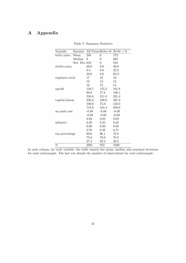
Selected summary statistics for the Enterprise dataset are shown in Table 5. 80% of firms weresmall in size (5-19 full-time permanent employees); 19% were medium sized (20-99 employees)and 1% of firms had more than 100 employees. The (mean) average age of the firms is 14 years.Less than 1% of the firms were foreign owned but roughly 2% of the sample engaged in some formof international trade8. 25% of firms received government provided water in their productionprocess, the figure for electricity was 2%. On average, the establishments operate for 62 hoursper week, 3 of which are spent by senior managers dealing with government regulations.

The average annual cost of dealing with requirements imposed by the government was�464,000,of which �48,500 was spent on external consultants used to deal with regulations. 83% of firmswere visited, inspected by, or required to meet tax officials in the previous year, and firms tookan average of 16 hours to fill in all forms and requirements to pay local taxes. The averageamount of sales that firms reported for tax purposes was 70%, compared with 61% of employeesreported for tax purposes. The average level of total employment was 17 workers. 9% of firms

81.1% of firms solely imported; 0.45% of firms solely exported; and 0.15% of firms engaged in both importingand exporting

10

Table 4: Variables

Variable Type Variable Name DefinitionMeasures OfBribery (ES &NBS)

bribe dummy Dummy=1 if firm reported a positive amount inbribe, 0 otherwise

bribe naira Amount of bribe in ‘000 Nairaebribe naira Amount of bribe per employee (in ‘000 Naira)

Measures OfControl Rights(ES)

infraserv Index (0-2) of public goods (water + electricity)acquired from government

tax percentage Percentage of sales declared for tax purposes

Measures OfBargainingPower (ES)

eprofit (Sales minus Operating Costs) Per EmployeeCapital labour Value of vehicles, machinery, and equipment per

employeeun sunk cost Measure Of Capital Mobility. The residual from:

resaleireplacei

= γ0 + γ1 ∗ log(age) + κialternative return un sun cost×capital stock

Measures OfControlRights/MeetingsWith PublicOfficials(NBS)

Customs clearing goods through customsRWC obtaining road worthy certificatesGov. procurement of goods and services from govern-

mentBus. Lic. obtaining business licenses and permitsPriv. procurement of goods and services from private

companiesEnviro getting clearance for environmental or sanitary

regulationsResidence residence and work permitsVehicle vehicle registrationsPolice police investigationsTraffic traffic offencesCourt contact with the court

had their financial statements checked by an external auditor and 3% of business owners had auniversity degree.

Average sales declined from 4 years previously to the year before the survey was taken,from �11.3 million to �8.4 million. The average value of machinery vehicles and equipment forthe entire manufacturing sample was �3.4 million. The average annual cost of electricity was�148,000.

6.1 Bribe Reporting

Results show that 51% of companies admitted to paying a bribe. The sample contained no non-respondents to the bribery related question. Amongst companies that reported a positive bribe,the average amount paid was �572,0009 per year with a median of �264,000 (£1050). Thiscorresponds to �40,000 per employee (or 6% of operating costs). Looking at the entire samplereduces these averages to �294,000; �20,000 per employee; and 3.3% respectively. Out of thefirms that reported a positive bribe amount; 22% reported this in Naira and 78% reported thisas a percentage of sales.

Table 5 shows summary statistics of the main control rights and bargaining variables for allfirms. The majority of firms who reported a positive bribe chose to report in terms of salespercentage (802 versus 227). Student’s t tests show that firms reporting in terms of sales reportsignificantly higher values of bribe payments, bribe payment per employee, profit and amountof moveable capital than Naira reporters. While Naira reporters declare a larger proportion oftheir sales for tax purposes and engage in more international trade than sales reporters10.Thereare no significant differerences, however, in their number of employees; capital per worker; or

9The equivalent of £2270 in October 2007(£1:�251.97)10Results for bribe; bribe per employee; moveable capital; and tax percentage are significant at the 1% level of

significance. The result for international trade is significant at the 5% level.

11

receipt of public services. The median bribe for the firms reporting bribes in Naira amounts were�50,000 whilst this value for sales reporters was �390,000.

Chemical manufacturing and wood manufacturing had the highest within-industry percentageof bribe paying firms11 (57% and 56% respectively). Electronics and garment manufacturing werethe least graft-intensive industry subsectors with 17% and 43% firms reporting bribes in eachindustry respectively12. The most bribe-intensive states were Benue; Taraba; and Yobe, witheach state having all of its firms admitting to paying some bribe. Lagos and Cross River statehad the lowest percentage of bribing firms (19% and 27% respectively).

The correlation matrix (ommitted) shows a statistically significant positive relationship be-tween the receipt of public services (“infraserv”) and the payment of bribes (“bribe dummy”),with a correlation of 0.07 which is significant at the 5% level. The percentage of sales reportedfor tax purposes (“tax percentage”) is also significantly related to the payment of bribes, with acorrelation of 0.1 which is significant at the 1% level. Both variables are also significantly pos-itively correlated with the amount of bribe paid (0.08 [1%] and 0.06[5%], respectively). Profitsand size of firm (employees) are also positively correlated with the bribe payment (0.3 and 0.2,respectively, both significant at the 1% level).

6.2 First Stage Estimations

Probit estimations were run to estimate the propensity to bribe. Marginal effects from theseestimations are shown in Table 6. The dependent variable in these models is a dummy in-dicating whether or not the firm paid a bribe. The variable “infraserv′′ is an index from0-2 indicating whether or not the company is in receipt of public services from the govern-ment. “tax percentage′′ denotes the percentage of sales declared, by the company, for taxpurposes. These two variables are the two main control rights variables. “eprofit′′ is profitper employee; “capital stock′′ is the resale value of machinery, vehicles, and equipment; and“alternative return′′ is the degree of capital mobility (described in Section 5). The base-line model uses only these variables as control variables. The augmented model includes adummy indicating whether the government is a principal buyer of the output of the company,“gov customer′′; and a variable denoting the average amount of time per week spent, by thesenior manager, dealing with government regulations, “regulation realtime′′. The further aug-mented model (Augmented+) includes regional and manufacturing sub-sector dummies.

The two main control rights variables, infraserv and tax percentage, enter positively andsignificantly, at the 1% level, in all first stage estimations. The marginal effects suggest thatrequiring 1 more type of public service from the government is associated with an increasedprobability of bribing of 6 percentage points. Similarly, every increase in the percent of salesthat is reported for tax purposes is associated with an increased probability of bribing of 0.2percentage points. These results suggest the intuitive idea that interaction with governmentemployees is associated with an increased risk of paying a bribe.

Results for the bargaining variables tend to confirm the conceptual framework. The coeffi-cients on these variables are all relatively small. Displaying them at 3 decimal places renders allof the coefficients to be zero. This suggests that observables such as profit and capital have noimpact on whether or not a firm pays a bribe. This goes slightly against the idea that those whopay bribes are the firms who are most willing and able to pay. It seems that the occurrence ofbribery occurs randomly amongst the profitable and the less profitable firms. The coefficientson the bargaining variables are all zero and not statistically different from zero, which confirmsthe conceptual framework since the bargaining variables do not enter into Equation (3.0.1).

11Excluding “Other Manufacturing” with a high of 67% of firms reporting graft.12Only 0.3% of the sample (6 firms) were from the electronics manufacturing sector

12

Having the government, or a government agency, as the principal buyer of the establishment’soutput is associated with an increased probability of paying of bribe of 0.21 probability points.This effect is significant in the augumented model at the 5% level. Also, an extra hour spentdealign with government regulations is linked with a 1 percentage point increase in the chanceof bribing.

All models have significant chi-squared values. A Wald test for the null hypothesis that thecoefficients on the control rights variables are equal to zero rejects the null at all traditionalsignificance levels. A similar tests for the bargaining variables fails to reject the null of a zerocoefficient on all of the bargaining variables. This provides more support for the idea that thepropensity to bribe is not necessarily determined by a firms profit but by required interactionswith government officials. A Wald test for the equality of the industry sub-sector dummies failsto reject the null of equality across manufacturing sub-sectors. This suggests that there is notmuch variation across the different industries in the propensity to bribe. A similar test for theindustry subsectors rejects the null hypothesis. Therefore, there appears to be regional variationin the bribing of public officials but no industry variation.

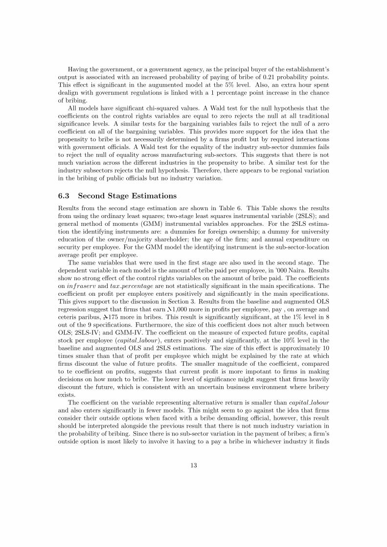
6.3 Second Stage Estimations

Results from the second stage estimation are shown in Table 6. This Table shows the resultsfrom using the ordinary least squares; two-stage least squares instrumental variable (2SLS); andgeneral method of moments (GMM) instrumental variables approaches. For the 2SLS estima-tion the identifying instruments are: a dummies for foreign ownership; a dummy for universityeducation of the owner/majority shareholder; the age of the firm; and annual expenditure onsecurity per employee. For the GMM model the identifying instrument is the sub-sector-locationaverage profit per employee.

The same variables that were used in the first stage are also used in the second stage. Thedependent variable in each model is the amount of bribe paid per employee, in ’000 Naira. Resultsshow no strong effect of the control rights variables on the amount of bribe paid. The coefficientson infraserv and tax percentage are not statistically significant in the main specifications. Thecoefficient on profit per employee enters positively and significantly in the main specifications.This gives support to the discussion in Section 3. Results from the baseline and augmented OLSregression suggest that firms that earn �1,000 more in profits per employee, pay , on average andceteris paribus, �175 more in bribes. This result is significantly significant, at the 1% level in 8out of the 9 specifications. Furthermore, the size of this coefficient does not alter much betweenOLS; 2SLS-IV; and GMM-IV. The coefficient on the measure of expected future profits, capitalstock per employee (capital labour), enters positively and significantly, at the 10% level in thebaseline and augmented OLS and 2SLS estimations. The size of this effect is approximately 10times smaler than that of profit per employee which might be explained by the rate at whichfirms discount the value of future profits. The smaller magnitude of the coefficient, comparedto te coefficient on profits, suggests that current profit is more impotant to firms in makingdecisions on how much to bribe. The lower level of significance might suggest that firms heavilydiscount the future, which is consistent with an uncertain business environment where briberyexists.

The coefficient on the variable representing alternative return is smaller than capital labourand also enters significantly in fewer models. This might seem to go against the idea that firmsconsider their outside options when faced with a bribe demanding official, however, this resultshould be interpreted alongside the previous result that there is not much industry variation inthe probability of bribing. Since there is no sub-sector variation in the payment of bribes; a firm’soutside option is most likely to involve it having to a pay a bribe in whichever industry it finds

13

itself in. This is one reason why the coefficient on alternative return only enters significantly in 3models. A further explanation is provided when an F-test for the equality of industry sub-sectordummies is conducted in the Augmented+ model. This test fails to reject the null of equalityof the bribe amount across different industry sub-sectors. This result suggests that the firm’soutside options would involve it paying roughly the same amount of bribe payment to anotherpublic official in a different industry, therefore the small and weakly significant coefficient on thevariable for alternative return can be explained by the fact that the outside options are not toodissimilar from the present option.

The coefficients on the government as the primary purchaser of the company’s output; and theamount of time spent dealing with government regulations enter insignificantly into the models.This supports the conceptual framework and adds more weight to the idea that the amount ofbribe paid is solely a function of the firms ability to pay; willingness to pay; and outside optionsrather than the nature of a firm’s meetings with public officials. An F-test on the regionaldummies rejects the null of equality; suggesting that there is regional variation in the amount ofbribe paid. The first-stage F-Statistic is significant in all IVs; suggesting that the instrumentsare not weak. A Durbin-Wu-Hausman test of endogeneity fails to reject the null of exogeneityof the profit variable. This suggest that one can have confidence in the OLS estimates in thisTable. All of these models are statistically significant.

7 Results - NBS

This section augments the previous results by including data from the NBS survey into theanalysis. The previous analysis does not distinguish between the reasons for bribery but insteadspecifies a number of general activities that might require a bribe. Firms were asked whetherpayments were made with regard to “customs, taxes, licenses, regulations, services etc”. Onone hand, asking a question in this manner might attract a higher estimate of the proportionof bribing firms i.e. asking if a firm paid a bribe for a number of activities might increase thereporting of bribery. On the other hand, this measure does not distinguish between bribes paidfor different activities. Therefore, any conclusions based on this data might give a biased view ofthe business environment in Nigeria: a large proportion of firms might have paid a bribe in orderto avoid punishment for an offence committed, rather than to bypass cumbersome regulation. Inorder to get a better view of the nature of bribe payments , the NBS data asks specific questionsconcerning what bribes were paid for. This data allows for an analysis into the processes whichattract the highest proportion of bribes.

Table 8 presents summary statistics for the NBS dataset. This table shows information onmeetings with public officials; and bribing of public officials for: all firms; those who met withpublic officials; those who bribed public officials. In this setup, a firm manager has to met witha public official in order to bribe a public official. Therefore, not meeting a public official is aperfect predictor of not bribing; and bribing an official implies that a meeting must have takenplace. There are a total of 11 meeting types asked about in this dataset, these are shown inTable 3. Results show that 37% of firms met with a public official. Managers who met with anofficial did so, on average, for 4 out of the 11 reasons asked about in the questionnaire. Out ofthe managers who met with an official 36% of them paid a bribe to an official. Bribing firms metwith an average of 4 officials and bribed 3 officials. The mean bribe value for the sub-sample ofbribing firms is �3,400.

Probit estimations were run on the propensity to bribe. The impact effects are shown inTable 9. The dependent variable in this table is a dummy equal to 1 if the firm admitted payingany type of bribe (specific or general). The variables in the table are dummy variables denoting

14

the different types of officials that the firms met with. These can be treated as control rightsvariables with the exception of the variable denoting procurement of goods and services fromprivate companies. The models also control for the size of firm; age; and foreign ownership.Models 1 to 11 show the partial impact effects of each control rights variable on the probabilityof paying a bribe; the full specification includes all control rights variables.

All variables enter positively and significantly at the 1% level in their respective partial effectsmodels, with the exception of the variables representing: the procurement of goods and servicefrom private companies; and contact with the court. Thus, in line with the conceptual framework,there is a positive relationship between meeting a public official and paying a bribe. The largestimpact effect is found in model 10 which measures the partial effect of meeting with officialsbecause of traffic offences on the propensity to bribe. Doing so leads to an increased probabilityof paying a bribe equal to 0.603 probability points, on average and ceteris paribus. The secondlargest impact effect (0.375) is associated with meeting officials for police investigations. Theseresults tend to be consistent with the results of surveys and research within and outside Nigeriawhich suggests the police force, who also deal with traffic offences, is one of the most corruptpublic institution. The coefficient on the variable for traffic offences maintains its sign andsignificance when entered into the full specification. A Wald test of equality of the coefficientsrejects the null of equality at the 1% level, giving more weight to the argument of heterogeneousofficials.

8 Robustness Checks

The Section shows the results of the misclassification adjusted probit model for the first stageestimation of the ES data; and for the estimation of the NBS data. Table 10 shows results for themarginal effects from the baseline probit specification; and the baseline HAS-Probit specificationusing the ES data. The marginal effects do not change by a relatively large amount. As expected,the marginal effects on the probability of bribing from HAS Probit model are larger than theordinary probit model. The model remains significant when allowing for misclassification. Thelog-likelihood function returned an estimate of the probability of observing a false negative of21.9%. In other words, the probability of observing a report of zero bribes when in fact thecompany did pay a bribe is 0.219.

Impact effects from the HAS-Probit model on the NBS data are shown in Table 11. All ofthe coefficients have the same sign and the majority of them keep their significance. Out of thesignificant coefficients, the ones relating to traffic offences and police investigations once againhave the largest magnitudes. The results from prevously are seen in the HAS-Probit model asthe coefficient for traffic remains significant and is also the largest coefficient in the full model.

9 Comparing The Two Datasets

Firms in the Enterprise Survey showed a greater willingness to report bribery than those in theNBS survey. 51% of firms in the ES reported a positive bribe payment compared to 27% of theNBS sample. When focusing on manufacturing firms, the data seems to tell a similar story: 51%of ES manufacturers reported paying a bribe compared to 23% of NBS manufacturers (Tableommitted).

Focusing on the average level of bribe payments for all firms and bribe paying firms: theaverage bribe payment for the ES full sample (All Industries) was �293,400. Focusing on bribepaying firms alone raises this average to �562,200. There was also a wide disparity in the averagereported bribe payments between companies who report in terms of the absolute Naira amount

15

and those who choose to report their bribe payments as a percentage of sales. Focusing on firmswho reported paying a bribe the average reported bribe payments amongst sales reporters was�690,000; whereas those who revealed their bribe as a Naira figure reported paying, on average,�73,700. The distribution of bribe payments for firms in the NBS sample appears to be closerto that of the ES Naira reporters: the average reported bribe payment for this sample of firmsis �53,400. These results are also seen when looking solely at the manufacturing industry inNigeria. Average bribe payments for bribing sales reporters, Naira reporters, and NBS firms ,respectively, are: �710,300; �85,500; and �77,900.

The regional distribution of bribe incidence and the average bribe payments amongst bribingfirms per state is shown in Figure 1. The upper part of the diagram shows the proportion of bribereporting firms across different states in Nigeria for all firms of the ES sample. Results indicate arelatively higher prevalence of bribing firms in the South-South region of Nigeria. These includeRivers, Imo and Akwa Ibom and these results are consistent between both datasets. Kogi Statealso has a relatively high prevalence of bribery. Focusing on the average bribe payments for bribereporting manufacturers, companies in Adamawa appear to consistently report a higher bribepayment in both samples.

9.1 Perceptions Versus Reality

Perception based indicators of corruption can suffer from bias [Carlin & Seabright , 2007]. Moreproductive companies have a higher valuation of the business environment than less productivefirms. Accordingly, any constraint to the business environment serves as a higher cost to theiroperations compared with less productive companies. Following from this, relatively more pro-ductive firms are more likely to complain about constraints to the business environment thanless productive ones. Therefore creating a bias in perception indices of the state of the businessenvironment.

One possible solution to this, in the case of bribery, is to compare subjective reports on theextent of corruption to the actual reported bribe payments. If all firms face the same businessenvironment then, in the absence of misreporting and bias, companies in areas where bribery ismore pervasive should report this in their subjective valuations of the business environment.

Companies in the Enterprise Survey were asked: “Do you think that the following presentany obstacle to the current operations of your establishment?” with “corruption” being one ofthe options.13

Responses to these questions show some evidence that businesses are revealing somethingwhen they give subjective evaluations of the business environment. Only 39% of those who saidthat corruption presented “no obstacle” to business operations paid a bribe to deal with businessregulations whereas 69% of those who reported that corruption posed a “very severe obstacle” tooperations reported paying a bribe. The values for the proportion of bribing firms increases asone moves from ‘no obstacle’ to ‘very severe obstacle’. The proportion of bribing firms decreasesas one moves from the ‘moderate obstacle’ group to the ‘major obstacle’ group, however, thisdifference is not statistically significant at the 10% level. This pattern is also reproduced in theNBS dataset.

13To be sure, the term “corruption” encompasses a number of acts, so companies might have been referring tobribery amongst other things when responding to this question. However, the data suggests a positive relationshipbetween the occurrence of bribery and the other elements that come under the term “corruption”.

16

9.2 Instigator Of The Bribe Transaction

Finally, Table 12 helps to shine light on the instigator of the typical bribery transaction. This isdone by using a set of categorical response questions which ask the firms how frequently bribesare: 1) demanded from; and 2) offered to; public officials. Firms were given a choice of responses:never happens; not very frequent but not unusual; fairly frequent; and very frequent. The basecategory used in Table 12 is “never happens”. The first three columns of coefficiets show resultsfrom the model that uses the offering of gifts as the dependent variables; the second set ofcoefficients, on the right hand side, show results from the model describing the determinants ofbring asked to pay a gift to a public official.

Committing a traffic offence is associated with an increased relative risk of reporting that firmsoffer bribes to public officials “very frequently” relative to reporting that “this never happens”.In addition to an increased risk of offering an official an informal payment, being involved in atraffic offence increases the log of the relative-risk of reporting that officials demand bribes veryoften relative to not at all. This result also holds for the other two categories. The coefficientson traffic offences are, on average, larger and have greater statistical significance than the othercoefficients. It therefore seems that traffic offences attract bribe demands from public officialsand propel bribe offers from firms. Furthermore, the coefficients in the model describing thedeterminants of being asked to pay a bribe are larger and more statistically significant than thecoefficients in the model that describes the offering of bribe payments by firms. Therefore, itappears that, according to firms, public officials demand bribes to a greater extent than firms offerbribes; however, there is evidence to suggest that both phenomena are present in the businessenvironment in Nigeria.

10 Conclusion

This paper has shown evidence for both the control rights hypothesis and the bargaining hy-pothesis amongst manufacturing companies in Nigeria. Despite the potential sensitivity of thetopic, various methods have been used in order to extract honest responses about bribery fromfirms. Whilst still potentially measured with error, these responses assist in the analysis of thenature of bribe payments amongst Nigerian firms.

The occurrence of bribery seems to be positively related to interactions with governmentofficials. Results also suggest that the size of the bribe is determined by factors representinga firm’s ability to pay and outside options. These findings are robust to different econometricspecifications. Results point to the notion that firms pay bribes because they desire items and/orservices in order to carry out their business,which sometimes require them to pay informal gifts inorder to either receive them or speed up the process of receiving them [Leite & Weidemann , 2002].In the case of Nigeria, 65% of manufacturing firms state that the government’s interpretation oflaws and regulations are consistent and predictable. 51% of firms report a positive bribe amountthat is required in order to speed the process of regulations.

By distinguishing between the different purposes for which a bribe was paid, this investigationwas able to analyse which activities were more likely to attract bribes. The data presented inthe preceeding analysis builds on the literature that analyses specific reasons for these payments.

Varaibles denoting interactions with public officials were found to be positively related withthe propensity to pay a bribe. Firm specific characteristics such as profit and capital stockwere found to be relatively good indicators of the level of bribe paid. On average, firms withhigher profits pay larger bribes. Earning 1,000 Naira (per employee) more, is associated withan increased bribe payment of 175 Naira (per employee), on average and ceteris paribus. Ev-idence was found for regional heterogeneity in the payment and size of bribe after controlling

17

for observables. Regions with higher probability of bribe payment seem to have a lower averagebribe payment (consistent with Shleifer & Vishny (1993); Svensson (2003)). Furthermore, thepropensity to pay a bribe, conditional on meeting a public official, depends on which type ofpublic official a firm meets with (consistent with Hunt (2006); Hunt & Laszlo (2012)). Meetingwith an official because of a traffic offence has the greatest impact effect on the probability ofpaying a bribe; and the relative-risk of being asked to pay a bribe by a public official.

Further work can build on this study by investigating whether informal payments have asignificant effect on the future profitability and competitiveness of companies. This will allowfor a better interpretation of the effect that expected future profits has on the level of bribepaid. Work that investigates the effect of competitors paying bribes on the firm’s profitabilityand propensity to bribe would also add to the analysis of the supply of bribes.

References

Azfar, O. and Murrell, P. (2009), Identifying Reticent Respondents: Assessing The QualityOf Survey Data On Corruption And Values. Economic Development And Cultural Change. 57,(2), pp. 387-411.

Carlin, W. & Seabright, P., (2007). Bring Me Sunshine: Which Parts Of The Business Envi-ronment Should Public Policy Try To Fix? Annual World Bank Conference On DevelopmentEconomics. Bled, Slovenia.

Clarke, G.R.G.(2011), How Petty Is Petty Corruption? Evidence From Firm Surveys InAfrica. World Development 39, 7: 1122-1132.

Cole, S. & Tran, A., (2011). Evidence From The Firm: A New Approach To Understand-ing Corruption. In S. Rose-Ackerman and T. Soreide (eds.) International Handbook On TheEconomics Of Corruption (Vol II).

Clist, P., (2011). 25 Years Of Aid Allocation Practice: Comparing Donors And Eras. CreditResearch Paper.

Delavallade, C. (2011), What Drives Corruption? Evidence from North African Firms, Work-ing Papers 244, Economic Research Southern Africa.

De Rosa, D., Gooroochurn, N. & Gorg, H., (2010).Corruption And Productivity Firm-Level Evidence From The BEEPS Survey. Kiel Working Papers 1632. Kiel Institute For TheWorld Economy.

Fan, C.S., Lin, C. and Treisman, D.(2010), Embezzlement Versus Bribery. National Bureauof Economic Research Working Paper 16542.

Fisman, R. & Svensson, J., (2007). Are Corruption And Taxation Really Harmful To Growth?Firm Level Evidence. Journal Of Development Economics. Volume 83, Issue 1, pp.63-75.

Fisman, R. & Miguel, E. (2007). Corruption, Norms And Legal Enforcement: Evidence FromDiplomatic Parking Tickets. Journal of Political Economy. 115, 6, pp. 1020-1048.

Foreign Corrupt Practices Act (1977). Unlawful Corporate Payment Act Of 1977. HouseOf Representatives. Report No. 95-640.

Greene, W.H.(2003), Econometric Analysis. Fifth Edition. Pearson Education Inc. USA.

18

Hausman, J.A.(1978), Specification Tests In Econometrics. Econometrica. 46, pp. 1251-1271.

Hausman, J.A. and McFadden, D.(1984), Specification Tests For The Multinomial LogitModel, Econometrica. 52, pp. 1219-1240

Heckman, J.(1979) Sample Selection Bias As A Specification Error. Econometrica. 47,1, pp.153-161.

Hellman, J.S.,Jones, G., and Kaufmann, D., (2000) September. “Seize the state, seize theday”: state capture, corruption, and influence in transition. Policy research working paperseries 2444. World Bank.

Human Rights Watch, (2010). ”Everyone’s in on the Game”: Corruptionand Human Rights Abuses by the Nigeria Police Force. Available Online:http://www.hrw.org/en/reports/2010/08/17/everyone-s-game-0. Accessed: 20th September2012.

Hunt, J., (2004). Trust And Bribery. The Role Of The Quid Pro Quo And The Link WithCrime. NBER Working Paper Series. Working Paper 10510. NBER. Cambridge, MA.

Hunt, J., (2006). Why Are Some Public Officials More Corrupt Than Others? In SusanRose-Ackerman (ed.) International Handbook on the Economics of Corruption. Edward Elgar.Northampton, M.A.

Hunt, J., (2007). How Corruption Hits People When They Are Down. Journal Of DevelopmentEconomics. Volume 84, Issue 2, pp. 574-589.

Hunt, J., (2008) The Contrasting Distributional Effects Of Police And Judicial Corruption.Annual Bank Conference On Development Economics.

Hunt, J. & Laszlo, S., (2012). Is Bribery Really Regressive? Bribery’s Costs, Benefits, AndMechanisms. World Development. Volume 40, Issue 2, pp.355-372.

Johnson, S., Kaufmann, D., McMillan, J. & Woodruff, C., (2000). Why Do Firms Hide?Bribes And Unofficial Activity After Communism. Journal Of Public Economics. Volume 76,Issue 3, pp.495-520.

Kaufmann, D. & Wei, S.J., (1999). Does “Grease Money” Speed Up The Wheels Of Com-merce?. NBER Working Paper.

Knack, S. & Keefer, P., (1997). Does Social Capital Have An Economic Payoff? A Cross-Country Investigation. Quarterly Journal Of Economics. 112, 3, pp. 1252-1288.

Lambsdorff, J.G., (1998) An Empirical Investigation Of Bribery In International Trade. TheEuropean Journal Of Development Research, 10, 1, pp.40-59.

Lambsdorff, J.G., (1999). The Transparency International Corruption Perceptions Index 1999:Framework Document. Transparency International.

Lambsdorff, J.G., (2007). The Methodology Of The Corruption Perceptions Index 2007.Transparency International.

Leite, C. and Weidmann, J., (2002): Does mother nature corrupt? In: G.T. Abed and S.Gupta, eds. (2002) Natural resources, corruption, and economic growth. Governance, corrup-tion, and economic performance. International Monetary Fund. pp. 159-196.

19

Lin, T. & Schmidt, P. (1984). A Test Of The Tobit Specification Versus An AlternativeSuggested By Cragg. The Review Of Economics And Statistics. Vol. 66, No. 1, pp.174-177.

Maddala, G.S., (1983), Limited-Dependent And Qualitative Variables In Econometrics. Cam-bridge University Press. USA.

Mauro, P., (1995). Corruption And Growth. The Quarterly Journal of Economics. Vol. 110,No.3, pp. 681-712.

Mendez, F. and Sepulveda,F., (2010) What Do We Talk About When We Talk About Cor-ruption? Journal Of Law, Economics, and Organization, 26, 3, p.493

Puhani, P.A., (2000). The Heckman Correction For Selection And Its Critique. Journal OfEconomic Surveys, Vol. 14, pp.53-68

Ramey, V.A. and Shapiro, M.D., (2001). Displaced Capital: A Study Of Aerospace PlantClosings. Journal Of Political Economy. 109, 5, pp. 958-992.

Rand, J. and Tarp, F., (2010). Firm-Level Corruption in Vietnam. United Nations University- World Institute For Development Economics Research, Working Paper No. 2010/16.

Reinikka, R. and Svensson, J., (2003) June. Survey techniques to measure and explain cor-ruption. Policy research working paper series 3071. World Bank

Rose-Ackerman, S.,(1978). Corruption: A Study In Political Economy. Academic Press. NewYork.

Ross, L., Greene, D. and House, P., (1977).The “False Consensus Effect”: An EgocentricBias in Social Perception and Attribution Processes. Journal Of Experimental Social Psychol-ogy, 13, 3, 279-301.

Shleifer, A., and Vishny, R.W., (1993). Corruption. Quarterly Journal Of Economics, 108,pp. 599-617

Small, K.A. and Hsiao, C., (1985). Multinomial Logit Specification Tests. International Eco-nomic Review, 26,3, pp. 619-627.

Svensson, J., (2003). Who Must Pay Bribes and How Much? Evidence from a Cross Sectionof Firms. The Quarterly Journal of Economics. 118(1),pp. 207-230

The Laws Of The Federation Of Nigeria, (1990). Volume 5 Chapter 27:Criminal CodeAct, Chapter 12: Corruption and Abuse of Office.

Ufere, N., Perelli, S. Boland, R. & Carlsson, B., (2012). Merchants Of Corruption: HowEntrepreneurs Manufacture And Supply Bribes. World Development.

20

A Appendix

Table 5: Summary Statistics

Variable Statistic All FirmsBribe=0 Bribe > 0bribe naira Mean 294 0 572

Median 8 0 264Std. Dev.652 0 816

ebribe naira 20.6 0.0 40.00.5 0.0 22.249.6 0.0 63.3

employee total 17 18 1612 13 1216 18 14

eprofit 158.7 155.3 161.890.0 77.8 100.1216.8 211.8 221.4

capital labour 230.2 190.9 267.2100.0 75.0 125.0718.8 544.4 850.0

un sunk cost -0.88 -0.88 -0.89-0.88 -0.88 -0.890.03 0.02 0.03

infraserv 0.29 0.25 0.320.00 0.00 0.000.50 0.48 0.51

tax percentage 69.6 66.1 72.875.0 70.0 75.027.4 28.2 26.2

N 2001 972 1029

In each column, for each variable, the table reports the mean, median and standard deviationfor each (sub)sample. The last row details the number of observations for each (sub)sample.

21

Figure 1: Proportion Of Bribing Firms; And Average Bribe Amounts For Bribing Firms, ByRegion

22

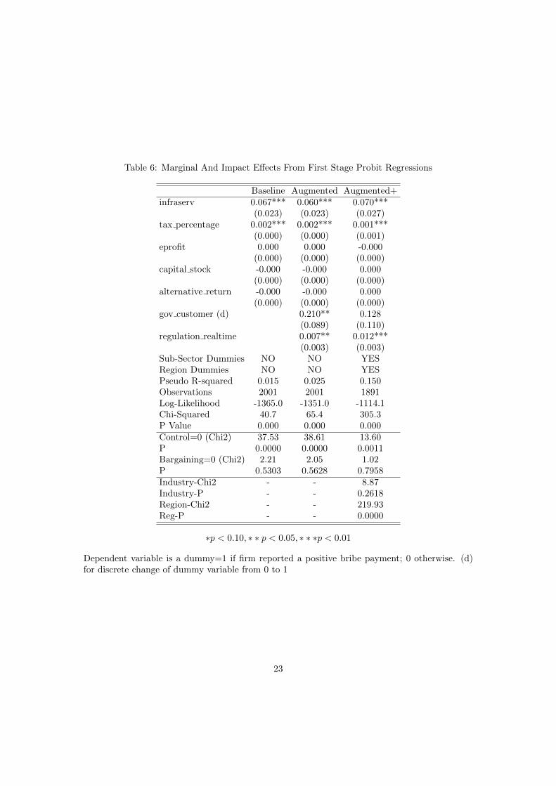
Table 6: Marginal And Impact Effects From First Stage Probit Regressions

Baseline Augmented Augmented+infraserv 0.067*** 0.060*** 0.070***

(0.023) (0.023) (0.027)tax percentage 0.002*** 0.002*** 0.001***

(0.000) (0.000) (0.001)eprofit 0.000 0.000 -0.000

(0.000) (0.000) (0.000)capital stock -0.000 -0.000 0.000

(0.000) (0.000) (0.000)alternative return -0.000 -0.000 0.000

(0.000) (0.000) (0.000)gov customer (d) 0.210** 0.128

(0.089) (0.110)regulation realtime 0.007** 0.012***

(0.003) (0.003)Sub-Sector Dummies NO NO YESRegion Dummies NO NO YESPseudo R-squared 0.015 0.025 0.150Observations 2001 2001 1891Log-Likelihood -1365.0 -1351.0 -1114.1Chi-Squared 40.7 65.4 305.3P Value 0.000 0.000 0.000Control=0 (Chi2) 37.53 38.61 13.60P 0.0000 0.0000 0.0011Bargaining=0 (Chi2) 2.21 2.05 1.02P 0.5303 0.5628 0.7958Industry-Chi2 - - 8.87Industry-P - - 0.2618Region-Chi2 - - 219.93Reg-P - - 0.0000

∗p < 0.10, ∗ ∗ p < 0.05, ∗ ∗ ∗p < 0.01

Dependent variable is a dummy=1 if firm reported a positive bribe payment; 0 otherwise. (d)for discrete change of dummy variable from 0 to 1

23

Table 7: Results - Regressions On The Amount Of Bribe

Base (IV-2sls)14 (IV-gmm)15 Aug (IV-2sls) (IV-gmm) Aug+ (IV-2sls) (IV-gmm)infraserv -3.536 -4.531 -0.358 -3.549 -4.336 -0.341 3.218 2.133 5.696*

(3.518) (4.573) (3.204) (3.543) (4.525) (3.200) (3.581) (4.233) (3.257)tax percentage -0.077 -0.075 0.157*** -0.060 -0.058 0.141*** -0.055 -0.049 0.000

(0.052) (0.054) (0.055) (0.054) (0.055) (0.054) (0.056) (0.058) (0.055)eprofit 0.175*** 0.201*** 0.156*** 0.175*** 0.195*** 0.150*** 0.160*** 0.227*** 0.063

(0.039) (0.072) (0.033) (0.039) (0.068) (0.033) (0.041) (0.066) (0.040)capital labour 0.017* 0.015* 0.020 0.018* 0.016* 0.021 0.012 0.007 0.020

(0.009) (0.009) (0.012) (0.010) (0.009) (0.013) (0.008) (0.006) (0.014)alternative return 0.001* 0.001 0.001 0.001* 0.001* 0.001 0.001 0.000 0.001

(0.001) (0.001) (0.001) (0.001) (0.001) (0.001) (0.001) (0.000) (0.001)gov customer 18.656 18.385 21.528 19.002 17.637 23.201

(16.169) (15.710) (16.456) (14.825) (13.345) (16.591)regulation realtime -0.493 -0.484 -0.206 0.093 0.057 0.343

(0.318) (0.321) (0.333) (0.386) (0.408) (0.386)Constant 17.367*** 13.579 20.182*** 17.391 14.778* 7.779

(5.996) (11.027) (7.213) (11.162) (8.142) (10.141)Sub-sector Dummies YES YES YESRegion Dummies YES YES YESF 6.278 6.610 .H0 : Exogenous .286 .3823 .193 .452 2.25 0.000P .593 .5364 .661 .502 .134 1.000First Stage F 85.79 119.85 57.81 67.82 25.16 15.73Adjusted R-squared 0.402 0.394 0.404 0.399 0.489 0.439Observations 1029 1029 1029 1029 1029 1029 1029 1029 1029Ind-F 1.39 8.93 9.59Ind-P Value 0.2042 0.2574 0.2128Reg-F 6.47 161.68 275.78Reg-P Value 0.0000 0.0000 0.0000

Dependent variable is bribe amount in ’000 Naira

∗p < 0.10, ∗ ∗ p < 0.05, ∗ ∗ ∗p < 0.01

24

Table 8: Summary Statistics Of Bribery And Meeting With Public Officials - NBS Data

(1) (2) (3)Bribery/ Meeting With Official

All Firms Met WithAn Official

Bribed AnOfficial

Met With An Official 0.37 1 1(Mean) Average Number Of Types OfOfficials Met With

1.66 (2.72) 4.43 (2.74) 4.20 (2.50)

Bribery Episode 0.14 0.36 1(Mean)Number Of Types Of BriberyEpisodes

0.44 (1.39) 1.16 (2.07) 3.20 (2.31)

Observations 331 124 45(Mean)Value Of Bribes (’000 �)(�) 0.616 (4.56) 1.65 (7.36) 3.43 (9.49)

The unit of observation is the firm. Standard deviations are in parentheses.

25

Table 9: Probit Estimations On The Propensity To Bribe - NBS Data (Impact Effects)

0 1 2 3 4 5 6 7 8 9 10 11 fullCustoms 0.309*** 0.153

(0.082) (0.107)RWC 0.226*** -0.162**

(0.068) (0.067)Gov. 0.308*** -0.047

(0.111) (0.084)Bus. Lic. 0.223*** 0.043

(0.077) (0.100)Priv. 0.140 -0.025

(0.104) (0.098)Enviro 0.311*** 0.094

(0.076) (0.107)Residence 0.168** -0.143***

(0.081) (0.052)Vehicle 0.333*** 0.317**

(0.068) (0.127)Police 0.375*** 0.142

(0.095) (0.125)Traffic 0.603*** 0.659***

(0.075) (0.096)Court 0.045 -0.154***

(0.102) (0.041)PseudoR-squared

0.098 0.150 0.135 0.126 0.127 0.104 0.153 0.112 0.176 0.151 0.297 0.098 0.383

Log-Likelihood

-145 -137 -139 -140 -140 -144 -136 -143 -132 -136 -113 -145 -99

Chi-Squared 34.2 50.1 49.2 46.4 45.6 39.7 51.9 37.5 61.9 46.8 84.4 34.1 104.6Reg-Chi-Squared

19.17 21.78 20.91 23.87 19.20 20.59 19.85 19.34 22.45 18.69 30.11 18.82 39.12

Reg-P Value 0.4 0.3 0.3 0.2 0.4 0.4 0.4 0.4 0.3 0.5 0.1 0.5 0.0

287 Observations. Dependent variable is a dummy variable equal to 1 if the firm reporting payinga bribe; 0 otherwise. Control vars include: size of firm, age of firm, foreign ownership.

∗p < 0.10, ∗ ∗ p < 0.05, ∗ ∗ ∗p < 0.01

26

Table 10: Misclassification Probit - Marginal Effects

BaselineMisc. Baselineinfraserv 0.067*** 0.086**

(0.023) (0.095)tax percentage 0.002*** 0.003***

(0.000) (0.002)eprofit 0.000 0.000

(0.000) (0.000)capital stock -0.000 -0.000***

(0.000) (0.000)alternative return -0.000 -0.000***

(0.000) (0.000)α1 - 0.219Pseudo R-squared 0.015Observations 2001 2001Log-Likelihood -1365.0 -1360.1Chi-Squared 40.7 26.9P Value 0.000 0.000

Dependent variable is a dummy variable equal to 1 if the firm reporting paying a bribe; 0otherwise.

∗p < 0.10, ∗ ∗ p < 0.05, ∗ ∗ ∗p < 0.01

27

Table 11: Misclassification Probit (Impact Effects)

0 1 2 3 4 5 6 7 8 9 10 11 fullCustoms 0.309*** 0.212*

(0.209) (0.491)RWC 0.421 -0.225*

(0.779) (0.484)Gov. 0.624 -0.065

(1.319) (0.949)Bus. Lic. 0.223*** 0.060

(0.195) (0.489)Priv. 0.449 -0.035

(1.139) (0.576)Enviro 0.311*** 0.130

(0.194) (0.485)Residence 0.168** -0.198

(0.213) (0.696)Vehicle 0.390 0.440***

(0.796) (0.465)Police 0.375*** 0.197

(0.236) (0.584)Traffic 0.822*** 0.914***

(0.643) (0.642)Court 0.045 -0.214***

(0.301) (0.650)α1 0.0000 .464 .506 0.0003 .0000 .0000 .147 .0000 .266 .0000 .0000 .279Log-Likelihood

-167 -157 -160 -162 -161 -165 -157 -164 -153 -157 -134 -167 -121

Chi-Squared 8.60 27.09 3.69 6.33 20.52 4.25 26.96 15.18 2.72 27.15 15.46 9.92 26.23P 0.0351 0.0000 0.4493 0.1755 0.0004 0.3730 0.0000 0.0043 0.6065 0.0000 0.0038 0.0418 0.0242

300 Observations. Dependent variable is a dummy variable equal to 1 if the firm reporting payinga bribe; 0 otherwise. Control vars include: size of firm, age of firm, foreign ownership.

∗p < 0.10, ∗ ∗ p < 0.05, ∗ ∗ ∗p < 0.01

28

Table 12: Relative Risk Ratios For The Instigator Of The Bribe Transaction

DependentVariable:

“A Firm Offers Gifts/Money To A Public Official” “A Public Official Asks a Firm For Gifts/Money”“not very frequentbut not unusual”

“fairly frequent” “very frequent” “not very frequentbut not unusual”

“fairly frequent” “very frequent”

Customs 4.387** 1.333 1.144 6.250** 3.904 0.999(3.171) (1.330) (0.916) (5.656) (3.365) (0.928)

Bus. Lic. 0.712 0.726 4.199* 0.494 0.845 9.894**(0.657) (0.618) (3.422) (0.423) (0.780) (10.879)

Vehicle 0.152** 0.086*** 0.477 0.055*** 0.248 0.118**(0.129) (0.073) (0.315) (0.052) (0.239) (0.126)

Police 2.956 7.600* 3.433 0.651 0.713 0.092(3.157) (8.140) (4.667) (0.614) (0.655) (0.153)

Traffic 7.187** 9.497*** 20.563*** 11.072*** 12.631*** 108.439***(5.567) (6.516) (15.546) (8.662) (9.457) (119.588)

Court 7.308* 0.254 0.769 10.483* 25.945*** 7.328(8.217) (0.396) (1.094) (12.722) (28.017) (10.948)

Constant 0.043** 0.239 0.000 0.169 0.379 0.000***(0.062) (0.257) (0.000) (0.185) (0.494) (0.000)

Base category: “never happens”. Control vars include: size of firm, age of firm, foreign ownership,regional dummies, RWC, Gov., Priv., Enviro, and Residence.

∗p < 0.10, ∗ ∗ p < 0.05, ∗ ∗ ∗p < 0.01

Figure 2: Reports Of “Similar Firms”

Informal Payments To “Get Things Done” Informal Payments To Acquire Government Contract

Payments To “Get Things Done” (by Size; Sector & Region) Payments To Acquire Government Contract (by Size, Sector & Region)

29

Legalize, Tax, and Deter: Optimal

Enforcement Policies for Corruptible Officials

Alfredo Burlando∗, Alberto Motta†

January 30, 2013

Abstract

Corruption of law enforcers remains a significant problem in many countries. We

propose a model where deterrence of a harmful activity (such as trade in illicit drugs)

is hindered by corruption, but standard anti-corruption policies might be too costly to

implement. We show that an alternative tax-and-legalize policy can yield significant

benefits, especially in poor countries with weak institutions and for activities that are

not too harmful. Using a tax-and-legalize scheme, the government reduces the cost

of implementing standard anti-corruption policies, easing the fight against corruption.

However, a tax-and-legalize policy could increase the equilibrium number of harmful

activities.

JEL Classification: D73, K42, O10, H21

Keywords: legalization, permits, law enforcement, corruption, incentives, self re-

porting, leniency program, collusion.

1 Introduction

The corruptibility of law enforcers remains a significant concern in many developing and

advanced economies. Among the possible anti-corruption policies, the economic literature

has mainly focused on compensation schemes that penalize corruption and reward honest

behaviors (Mookherjee and Png [1995], Mishra [2002], and Bose [2004]). While these policies

∗Corresponding author. University of Oregon, Department of Economics, Eugene, OR 97405, tel (541)346-1351, e-mail: burlando@uregon.edu†University of New South Wales, School of Economics, Australian School of Business, Sydney 2052, email:

motta@unsw.edu.au

1

have the potential to effectively limit corruption, their implementation has proven to be

unsatisfactory in many countries (Transparency International [2010]). What could explain

these failures? A reason may be that stamping out corruption is costly, and in some countries

tolerating it might be socially optimal (Besley and McClaren [1993], Acemoglu and Verdie

[2000], and Bac, and Bag [2006]).

The primary objective of this paper is to show that legalization is useful in cases where

traditional anti-corruption policies are costly to implement. In a setting where individuals

engage in harmful activities and bribe officers to avoid being sanctioned, we study the effect of

implementing a tax-and-legalize scheme. This scheme allows individuals to freely undertake

the sanctioned activity in exchange for the payment of a tax or reduced fine. We will show

that legalization changes the enforcement problem, turning it from one of apprehension

of sanctioned acts, to one of detection of tax evasion. However, the potential problem of

corruption remains: just as before, tax evaders can bribe audit officers. Yet, this paper will

demonstrate that legalization in some instances reduces the cost of implementing an effective

(and otherwise expensive) anti-corruption scheme, thus solving the corruption problem.

To show this point, we build a simple model of enforcement in which individuals generate

a social harm when engaging in a certain activity (such as pollution or dealing with illegal

drugs) that provides them with a private gain. The government hires officers to monitor

the population and fine miscreants, and can decide whether to allow bribery to take place

or, through appropriate incentives, ensure that officers never accept bribes. We model the

enforcement problem such that bribes lower deterrence but are otherwise efficient: they

generate a transfer from miscreant to officers that avoids socially costly bureaucracy and red

tape. This setup allows our model to obtain many expected predictions that conform with

the existing literature. For instance, we find that poorer countries are more likely to adopt

corrupt enforcement, because anti-corruption policies are more expensive at lower income

levels. We also find that countries that are more tolerant of corruption or with high red tape

levels are more likely to adopt corrupt enforcement regimes. More surprisingly, we find that

2

the corruptibility of officers imposes significant welfare costs precisely in countries with low

levels of wealth, where corruption is most likely to occur. At higher levels of wealth, on the

other hand, the corruptibility of agents matters less and less for welfare: the tools available

to the government are sufficiently flexible that corruption avoidance is inexpensive.

Given this model, we analyze the effect of a tax-and-legalize policy. Individuals have the

option to freely engage in the harmful activity, then pay a tax to the government. Since tax

avoidance is an option, tax evaders would still face sanctions once audited, and therefore can

still attempt to bribe officers. Thus, the corruption problem does not go away with a tax-

and-legalize scheme. However, those individuals who do pay the tax have acted legitimately,

and therefore need not bribe the tax enforcers. Whenever one individual pay the tax, there

is one less anti-corruption incentive that needs to be paid out. This makes anti-corruption

policies sufficiently cheap that, as it will be shown, are completely and comprehensively

adopted in a legalized regime. This is particularly useful when such policies are otherwise

costly, which occurs at low levels of wealth in the model, precisely where corruption is the

preferred policy. Our welfare predictions are therefore quite stark: poor countries where an

illegal activity begets corruption should legalize, regardless of how tolerant of corruption that

country is.

The use of a tax-and-legalize scheme does lead to a potentially unpleasant effect: in gen-

eral, we find that more individuals engage in the socially harmful activity when it is legal,

even when the activity is appropriately taxed. Unlike most prior (mostly empirical) litera-

ture, this is not due to changes in the demand function of consumers1, or motivated by the

introduction of a revenue concern to the government: our model keeps both demand function

and government revenue concern constant. Instead, the reason for the increase in the harm-

ful activity is that, absent legalization, there is too much enforcement (something that was

also previously noted by Mookherjee and Png [1995]). Correcting this over-enforcement is a

property of legalization that, in a political economy context, could be considered controver-

1 Empirically, legalization has been found to increase the quantity demanded of the previously illegalgood (Saffer, and Chaloupka, (1999), DiNardo and Lemieux (2001), and Anderson and Rees (2011)).

3

sial : while society is better off with higher levels of the harmful act and a lower government

budget, individual voters who easily observe the first and not the latter might reject legal-

ization. Over-enforcement is less likely to occur at very low levels of wealth and for activities

that are not too harmful, suggesting that legalization could be more appealing in developing

countries and for lesser illegal activities.

The theory presented here is empirically relevant, particularly (but not only) for the

regulation of illicit drugs. Many poor countries have already legalized narcotics that are

illegal elsewhere. For instance, chat, a narcotic plant, is freely traded, taxed, and consumed

in Ethiopia, Yemen and Somalia. It remains illegal elsewhere. Bolivia has legalized the sale

and consumption of coca leaves, although more processed and harmful forms (a category

that includes cocaine) remain illegal. The call for broader legalization of other illegal drugs

is being increasingly made in policy circles by prominent figures concerned with corruption.

In 2010 former president of Mexico Vincente Fox argued in favor of drug legalization, in part

on corruption grounds. The presidents of both Bolivia and Uruguay are actively pursuing

more lax legalization policies, against the wishes of many western countries.2

There are other instances of legalization or self reporting policies in areas where the

possibility of corruption is great.3 As part of a larger anti-corruption push, off-track betting

was legalized in Hong Kong in the seventies; the legalization eliminated an important source

of bribes for the police force, and police corruption was eliminated shortly after (Klitgaard

[1988]). While big game hunting is generally illegal in Africa, countries such as Malawi,

Tanzania and Zambia have adopted hunting permits as a form of legalization for a crime –

2The consumption and trade of cannabis has been legalized in many Western countries and US statestoo; such legalization is generally driven by considerations not directly considered here, such as incarcerationpolicies. Nonetheless, our model can explain this evidence. Our results suggest that legalization can beoptimal even in countries where effective anti-corruption policies are in place, especially for activities thatare not too harmful.

3Among the various voices in the debate over legalization of things other than drugs, it is worth mentioningBasu (2011) who recently suggested legalizing bribe giving, while keeping sanctions on bribe taking. Heobserved that, when the entire punishment from corruption is concentrated on the bribe taker, the bribegiver has an incentive to report the bribe exchange. Anticipating this, the bribe taker will be much lessinclined to take the bribe in the first place. While we model legalizing the underlying activity and not theact of bribing, both models hinge on providing an alternative outside option to the bribe giver.

4

poaching – that is difficult to control.4

More broadly, the scheme we present here extends beyond legalization, and fits into a

general class of models where corruption is reduced by empowering individuals to bypass

officials (Motta [2012], and Burlando and Motta [2013]). Such schemes are becoming in-

creasingly prevalent. In 2005, India introduced a Freedom of Information Act (the RTIA),

which allows citizens to inquire about any governmental activity–including the status of a

person’s own permit applications. Peisakhin (2012) and Peisakhin and Pinto (2010) showed

in randomized trials that RTIA requests provide an alternative way to petition for a permit,

which ultimately reduces bribe payments. Private companies in developing countries also

use such schemes to get around their own corruptible employees. In India, the tatkal system

was introduced by the phone company to provide people with an alternative to paying bribes

for quick phone line installations. The Bharat Sanchar Nigam company guaranteed speedy

connections to those willing to sign up and pay into the program. The same taktal system

was later adopted by the railways as a way for customers to avoid long waiting lists or pay-

ing bribes to intermediaries for a quick ticket. In many instances, self reporting can become

operational following a technological innovation. In Tanzania, customers could consume

electricity for years without ever paying their bills. This was quite common until TANESCO

introduced ‘smart’ electronic meters which require payment before supplying electricity, by-

passing the corrupt workers. This system was borrowed from the cell phone industry and

has been successfully adopted in the water, telecommunications and trash disposal sectors.5

The rest of the paper is organized as follows: after a discussion of the current theoretical

literature, section 2 discusses the model of enforcement sans corruption; section 3 studies the

effects of corruption; section 4 introduces the tax and legalize scheme. Section 5 concludes.

4That some legalization of wildlife hunting and trade can be helpful and beneficial for conservation isa concept that is not lost for several environmental groups. In their 2008 joint report, TRAFFIC and theWWF state that “Policies that criminalize the wild meat trade have not been effective to bringing it undercontrol...greater consideration of alternative management scenarios, including legalizing hunting and tradeof certain wild species for meat is therefore required” (Roe, 2008).

5Top-up systems or pre-paid services are different from self reporting in one important aspect: the clienthas no choice but to pre pay if he wants the service. In law enforcement, miscreants always have a choicenot to pay.

5

Relation to the literature There is a growing literature on the economics of corruption

and legalization in law enforcement, which is often referred to as self reporting. Under

self reporting, the harmful activity is illegal, and remains so. Kaplow and Shavell (1994)

introduced the idea of self reporting in law enforcement;6 in their model, self reporting saves

money by reducing the number of officers needed to monitor the population.7 These cost

savings hinge on the enforcement agency being able to separate self reporters from the rest

of the population, which is not generalizable to many contexts where legalization would be

useful. Polinksy and Shavell (2001) consider a setup similar to ours but do not explicitly

model the source of the deadweight losses from corruption, and do not explore the role of

self reporting in corruption.8

The model we present here can be thought of as a self reporting model, because individuals

carry out the harmful acts first, and only later declare the acts through the payment of

the tax. An alternative legalization scheme would have an individual having to purchase

a permit from a bureaucrat before engaging in the sanctioned activity. Technically, our

results would hold irrespective of the timing. However, in the context of the permit, the

corruption problem could arise anew: a bureaucrat could decide to hold up the issuing of

the permit in exchange of a bribe (see Bardhan [1997] for a thoughtful discussion). This

problem is avoided by our scheme because the acts can be reported after they have been

committed. In practice, we believe that this distinction is becoming less important: creative

use of freedom of information acts, as well as new technologies that allow for the remote

application of taxes, levies, and permit requests, help avoiding bureaucratic holdup. We also

sidestep another important distinction between legalization and self reporting, namely the

psychological effect of making an illegal activity legal (what Miron and Zwiebel [1995] refer

6The model in Kaplow and Shavell (1994) builds on Becker (1964). Malik (1993) also explored the theorybehind self reporting in law enforcement. See also Polinsky and Shavell (2000) for a more general discussionon the law enforcement theory in economic literature.

7The literature on self reporting highlights other relevant aspects of the policy in environments withoutcorruption. See Innes (1999, 2000, 2001). For leniency programs see Motta and Polo (2003) and Buccirossiand Spagnolo (2005).

8See also Rose-Ackerman (1994), Hindriks, Keen, and Muthoo (1999), Livernois and McKenna (1999),and Malik (1990).

6

to the “respect for the law” effect.) In light of this effect, the choice of how to frame the

policy might go well beyond a simple labelling or semantic issue.

Perhaps closest to our paper is Andrianova and Melissas (2008). Using a different setup,

they study when governments choose to legalize an activity when officers are corrupt. They

assume that once the activity is legalized, the government imposes no reduced fines or taxes,

and employs no enforcement. While this might be useful in some contexts–say, when choosing

zero tariffs to reduce corruption among import inspectors–their model cannot explain the

role of legalization in context where harm control remains important.

2 The model

2.1 Structure

There is a measure 1 of risk-neutral citizens who cause a harm to society of h > 0 by

committing an act that provides a private gain of x. The gain is distributed with a continuous

density function g(.), which is everywhere strictly positive over the support [0,∞). We

assume a continuous cumulative distribution function G(.) and, for simplicity, a constant

hazard rate function g(x)1−G(x)

= λ.9 Absent enforcement problems, a welfare maximizing

government would allow only those citizens whose private benefit is x ≥ h to carry out

the act. However, the act is not directly observable, and the government must engage in

costly monitoring and enforcement. To this purpose, the government employs a measure p

of officers. They are responsible for monitoring the population and reporting violators to

a court of law, which in turn imposes fines. Enforcement works as follows. Each officer

is randomly matched with a citizen, and the officer immediately learns whether the citizen

has carried out the sanctioned activity. The officer’s information is hard and verifiable in

a court of law. The officer can report the violation to the judiciary system, which levies a

fine f to the offender. The maximum level of sanction is f , which may be interpreted as an

individual’s wealth.

9All results in the paper are generalizable to a nondecreasing hazard rate function.

7

2.1.1 Corruption

A corruptible officer will consider accepting a bribe b from the citizen in exchange for her

silence. The size of the bribe is reached through a bargaining process. We assume that,

while miscreants are willing to pay any bribe that is less than the fine, i.e. b ≤ f , the bribe

cannot be as large as the fine:

Assumption (Corruption tolerance): the maximum agreeable bribe cannot be larger

than a fraction σ ∈ (0, 1) of the fine.

In our model, the assumption introduces a limit to deterrence in corrupt regimes in a straight-

forward way. It corresponds to the reality of many bribery situations, where the bribe giver

settles for a bribe that is much smaller than the full sanction. Theoretically, there are several

ways to explain this condition. At its simplest, the assumption states that the larger the

bribe payment demanded by an officer, the greater is the chance of detection (as in Emer-

son, [2006]). Bribes that are too large become either detectable to the press and scandalous

to society, while a relatively small side payment would be either undetected or acceptable.

Thus, our σ measures society’s tolerance for corruption. Societies that are intolerant (low

σ) find bribery unacceptable, and only small exchanges (that can perhaps be confused as

acts of kindness rather than corruption) are possible. On the other hand, countries that are

tolerant (high σ) have societies where gift exchanges (which can mask bribery) are common

or consider bribe payments as a way of life.10 In either case, a collusive agreement where

bribes are too high would be uncovered by the public as blatant corruption, the officer would

lose the ill-gotten wealth, and the offender would be made to pay the full fine f .11

10The prevalence of gifts exchange traditions allows individuals to mask corruption (Klitgaard, 1988), andsome societies may just be more accepting when someone offers bribes to public officials (Lambsdorff, 2007).

11There are other possible ways to explain our assumption. Even if miscreants’ ability to pay is greateror equal to the fine f , they might be unable to transfer more than a fraction σf of this wealth in bribes.This could come from the fact that the fraction (1−σ)f is held in assets that are not easily transferrable, orwhose ownership is hard to verify at the time of the bribe transfer, such as boats, landholdings, or residentialunits located in another location or country. While a corrupt officer might be unable to take possession ofthese assets, a government can reasonably be expected to find, confiscate, and sell these items. Second, theassumption is consistent with a model where part of the punishment is non-monetary in nature, wherein onlya fraction σ of the punishment is extracted in monetary form and the rest administered via revenue-neutralimprisonment. Finally, the assumption would arise in a model where bribe exchanges suffer transaction

8

As an anti-corruption measure, the government can offer bonuses or incentives i that are

paid when an officer reports an offender. Because acceptance of the bribe implies foregoing

the incentive, the officer will consider only bribes that have the following characteristic:

i ≤ b ≤ σf . The agreement on the bribe is reached through a bargaining process, with

weights to the officer of µ ∈ (0, 1). The equilibrium bribe is given by the following expression:

b(i, f) = min {(1− µ)i+ µf, σf} , (1)

that is, the bribe level is fully characterized by the incentive and the fine. Note that, regard-

less of how the bargain power is distributed between the two parties, corruption is eliminated

whenever the incentive level i meets or exceeds the following no-collusion condition:

i ≥ σf ≡ inc. (IC)

When i < inc, a bribe will be agreed upon, violations are not reported, and the government

neither pays incentives, nor receives any income from the fine. When i ≥ inc, no bribes are

exchanged, and therefore all violations are reported, all fines are levied, and all incentives

are paid.

2.1.2 Enforcement costs

Officers are risk neutral with reservation utility v, where v is strictly positive and finite. The

government must offer a salary package that, in expectation, leaves officers with at least

their reservation utility. Namely, the base wage w and incentive i must satisfy the following

participation constraint:

w + Pr(audit success) max[b(i, f), i] ≥ v (PC)

costs, similar to those existing in the literature of corruption (Tirole, 1992).

9

where max[b(i, f), i] represents the gains obtained from either the incentive or the bribe. In

addition, we assume that officers are shielded by some degree of limited liability.

Assumption (Limited liability): Officers’ wages cannot fall below a certain threshold:

w ≥ w ≡ 0. (LL)

Limited liability is one way to generate a “cost of corruption”; see Burlando and Motta

(2012) for an alternative modeling strategy that relies on risk aversion and that generates

very similar insights. The assumption is particularly important in the context of many de-

veloping countries, where bureaucrats and law enforcement officers are generally very poorly

paid, and often go unpaid. A less common occurrence is that they receive negative wages,

although there are documented circumstances (see Besley and McClaren [1993]) in which en-

forcement officers essentially pay superiors for the right to enforce (and collect bribes). Even

in those cases, it is likely that there is a limited liability constraint, with the minimum wage

somewhere below zero. Fortunately, our paper can be easily generalized to those situations.

We assume w = 0 for the sake of exposition.12

2.1.3 The government

We conclude the model setup by introducing a benevolent, welfare maximizing government

whose contribution of enforcement expenditures B on the larger total government budget

consist of wage payments net of revenues from fines. The budget process has two distortions.

First, the budget is raised through distortionary taxation from the citizenship. A budget B

costs society (1 + d)B, where d measures the size of the dead weight loss and is normalized

to d = 1.13 Second, the revenue generating process is subject to some bureaucracy and red

12Implicitly, a second limited liability assumption states that w+max(b, i)] ≥ 0. In equilibrium, there willnever be a case where bribes or incentives are negative, so the condition is never binding.

13This is a critical distinction between our approach of corruptible enforcement and the canonical ap-proaches of enforcement in Kaplow and Shavell (1994) or Polinsky and Shavell (2001), where the govern-ment budget does not include the revenues from fines collected and the effect of distortionary taxation.From this perspective, our framework is similar in nature to setups more commonly found in the literatureof corruption, such as in Besley and McClaren (1993) and Laffont and Tirole (1993).

10

tape, such that only a fraction α ≤ 1 of revenues are accounted for and can be utilized. The

remaining portion of fine income is destroyed by red tape. We understand α as a measure

of efficiency in a country’s government.14

The social welfare function depends on the type of enforcement regime (clean or corrupt)

and on the number of individuals who commit the sanctioned act. We denote by x the

expected sanction faced under a certain enforcement regime. x is also a handy measure of

effective enforcement and social harm. Welfare is

W (x; i, f, w, p) =

∫ ∞x

(x− h)g(x)dx−B(x; i, f, w, p), (2)

where the budget function B(x) will be further specialized in the next section. Note that the

enforcement regime is characterized by the optimal selection of four policies: the number of

inspectors, p; the base wage, w; the incentive pay, i; and the fine to miscreants, f .

Further assumptions and timing of the model The timing of the model works as

follows. First, the government announces the full set of policies. Agents observe these

policies and decide whether to engage in the harmful act. Then, officers randomly pick

agents for monitoring, discover whether there was harm, and either assess the fine or agree

on the bribe.

We make three additional assumptions on the parameter space, whose purpose is to keep

the analysis pertinent to probabilistic enforcement by avoiding possible corner solutions

where there is either perfect enforcement or no enforcement at all.

Assumption A1: f > h1+α− σ−α

λ(1+α)> 0

Assumption A2: f > v/σ

Assumption A3: f > h/σ

The assumptions essentially state that the maximum fines that a government can impose

are sufficiently large to be worthwhile for deterrence. Implicitly, they also state that the

14A modified version of costly imposition of fines is found in Polinsky and Shavell (2000).

11

social harm h is sufficiently large, relative to parameters. Our main results extend to the

case where corner solutions are considered, but the presentation would suffer and become

much more involved.

2.2 Benchmark: no corruption

We start with an economy where enforcement agents cannot collude and are always honest.

It follows directly that incentives need not be offered, and wage rates remain always at the

lowest level possible: w = v. Moreover, given that officers never accept bribes, a citizen that

commits the illegal act faces an expected sanction x = pf . The total quantity of crime is

1−G(pf), which is also the probability of a successful audit. In total, thus, the government

can expect to receive αpf [1 − G(pf)] in revenues from fines. With this characterization, it

is straightforward to derive the welfare function. This will take into account the level of

criminality, the wage bill, and revenues from fines:

Whonest(p, f) =

∫ ∞pf

(x− h)g(x)dx− pv + αpf [1−G(pf)]. (3)

It is readily observable that the optimal enforcement policy requires maximal fines f = f .

If fines are not maximal, the government can increase welfare by increasing the fines and

reducing the amount of officers such that the enforcement level x = pf remains constant.

The first and last term in equation (3) are a function of the enforcement level, and remain

unchanged. However, the term in the middle is the wage bill, which is thus reduced. We lastly

characterize the optimal size of the enforcement force, p∗. To determine p∗, differentiate (3)

with respect to p using f = f to obtain

∂Whonest

∂p= f(h− pf)g(pf)− v + αf [1−G(pf)]− αpfg(pf)f

This expression will be negative for p = 0 if v is large enough, so p∗ = 0 is possible. Moreover,

the expression can be positive for p = 1, so p∗ = 1 is also possible. To keep the model as

12

simple as possible, we always focus only on interior solutions: that is, we limit the parameter

space so that the government wants some enforcement, and ignore those instances where it

is optimal not to enforce, or to enforce every single case. Assumptions 1-3 guarantee this.

An interior solution must satisfy the first-order condition that ∂Whonest

∂p= 0. Making use of

the fact that the hazard rate g(x)1−G(x)

= λ is constant, the optimal enforcement force p∗ solves

p∗f [1 + α] = h−(

v

fg(p∗f)− α

λ

)(4)

The left side is the net social loss from deterring the marginal individual, who would have

obtained p∗f had he committed the act and society would have obtained expected revenue

from fines p∗fα. The left side is the net social gain from deterring the same individual, the

harm avoided minus the net enforcement cost of deterring him.

While we cannot characterize the solution to this equation in a closed-form solution, it

is evident that, for any given set of parameter values, the left hand side of the equation is

strictly decreasing in p while the right hand side is strictly increasing in p; the solution exists

and is unique.

In addition, p∗′h > 0, p∗′α > 0 and p∗′v < 0. The first derivative simply states that actions

that have larger negative spillovers receive more enforcement. The second derivative implies

that administrations that are more efficient at collecting fines (have higher α) have also

a higher enforcement level. The implication is that enforcement is affected by a revenue

concern. The final derivative shows that enforcement decreases with v, which measures the

cost of an agent.

3 Enforcement in the presence of corruption

We next consider the case where corruption is possible. In solving for the optimal enforcement

policy, it is useful to consider separately the case where incentives are sufficiently high so that

officers do not accept bribes, and the case where incentives are low and officers are corrupt.

We refer to these two situations as corrupt and clean, and we index these two regimes by

13

j = c, nc respectively.

3.1 Clean regime

To begin, suppose that the incentive provided is i ≥ inc. As above, officers do not accept

bribes, so that enforcement is x = pf and revenues from fines are αpf [1 − G(pf)]. On the

cost side, the government pays a base wage bill pw and an incentive pay i for each fine that

is levied. With these elements, the welfare function is given by

Wnc(p, w, i, f) =

∫ ∞pf

(x− h)g(x)dx− pw + p(αf − i)[1−G(pf)]. (5)

The government maximises this welfare function subject to the incentive constraint (IC), the

limited liability constraint (LL) and to the participation constraint (PC) which in this case

takes the form

w + i[1−G(pf)] ≥ v (PCnc)

Note that at least one or both participation and limited liability constraints must bind

in equilibrium. (When they do not, the base wage w can be reduced without affecting

the enforcement level, and welfare increases.) Which constraint will bind depends on the

parameters of the model. Regardless of which constraint binds at the optimum, the following

remark applies:

Remark 1 The optimal policy in the clean regime includes i = inc and f = f . Enforcement

is given by xnc = pf .

We describe the general argument for this remark here, leaving the full proof to be part of the

optimal policy in proposition 2. Incentives are generally costly to the government whenever

(PCnc) is slack, and revenue-neutral otherwise. Given that increasing the incentive above

inc does not serve any purpose in terms of promoting honesty, setting i = inc is always an

optimal response. A similar argument holds for the fine f . For any fine amount that is not

maximal, it can be shown that the government can achieve the same enforcement x = pf by

14

increasing f and reducing p, such that enforcement costs are (weakly) lower. Hence, setting

the maximal fine f = f is also optimal.

The clean regime (5) is similar to the benchmark, honest case. In fact, it is readily

observed that the two are identical and lead to the same welfare whenever (LL) is slack.

Once (LL) binds, benchmark welfare is unattainable and corruption is socially costly. We

can measure the cost of corruption Cnc(x) to be the difference in welfare between the clean

and the benchmark case, for any given enforcement level x, using f = f and i = inc.15

Formally, it is

Cnc(x) ≡ Whonest(x)−Wnc(x) =

0 for v ≥ vσ

p{σf [1−G(x)]− v

}for v < vσ,

where vσ ≡ σf [1 − G(pf)] is the value of market wages where (LL) binds exactly. This

threshold value is increasing in σ. In the top panel of figure 1 we simulate the model and

plot Cnc(x) against market wages v, for an arbitrary enforcement level, and for two values

of σ. Details on the simulation and the parameters used are in Appendix C. The cost of

corruption is zero for v > vσ. When countries are sufficiently wealthy or have sufficiently

strong institutions, the corruptibility of officers does not create distortions because the cost

of paying high incentives is entirely neutralized by lowering the base salary w. When market

wages are below vσ, the government cannot neutralize the high incentives costs, owing to

limited liability. The limited liability threshold is reached either because wages v are low, or

because of high tolerance for corruption σ, which increases the equilibrium bribe and raises

the incentive inc required to keep the officers clean. “Clean” enforcement becomes socially

costly, with the cost increasing the poorer the country or the more tolerant to corruption

the institutions are. Under plausible parameter values, our simulations suggest that the cost

15A comparison between the clean and the benchmark regime evaluated at their respective optimal pis discussed in the next session, when legalization is introduced. Comparing the regimes at their optimalpolicies does not allow us to account for the direct cost of corruption because the level of enforcement in thetwo regimes is allowed to vary.

15

of corruption can be substantial for sufficiently poor countries.

Optimal “clean” enforcement We are now left with characterizing the optimal interior

xnc in the clean regime. As it will be clear later in the discussion, Assumptions 1-3 prevent

corner solutions, while relaxing these assumptions would not change our results. For the sake

of exposition, define two market-wage threshold values v˜ncσ ≡ σf [1 − G( h1+α−σ −

σ−αλ(1+α−σ)

)]

and vncσ ≡ σf [1 − G( h1+α− σ−α

λ(1+α))]. The following proposition characterizes the optimal

policy.

Proposition 2 The optimal interior enforcement policy with high-powered incentives in-

cludes fines and incentives as defined in remark 1 and enforcement xnc as follows:

a. When v > vncσ , only (PCnc) binds, the enforcement problem is equivalent to the benchmark

“honest” case equation (3), and xnc is given by first order condition (4).

b. When v˜ncσ ≤ v ≤ vncσ , both (LL) and (PCnc) bind, and the enforcement level is xnc =

G−1(1− vσf

).

c. When v < v˜ncσ , (LL) binds, (PCnc) is slack, and the enforcement level is xnc = h1+α−σ −

σ−αλ(1+α−σ)

.

Proof. See appendix.

When v > vncσ (case a.), the incentives paid out are perfectly compensated by a reduction

in the base salary (i.e., the participation constraint binds), leading to zero expected rents to

officers, no welfare losses from corruption, and benchmark welfare. In case b., countries with

intermediate wealth (v ∈ (v˜ncσ , vncσ ]) optimally decrease the base wage w to the minimum level

allowed by limited liability. However, officers still earn zero rent: in expected value, they

obtain exactly their market wage v. The government achieves this at the cost of distorting

enforcement away from the benchmark level. In fact, the distortion is such that there is over-

enforcement with respect to the benchmark. Over-enforcement reduces the probability that

an officer earns rents, and causes a reduction both in harmful activity, and in the number

16

of times incentives are paid. This relaxes (PCnc) and thus prevents the officers from earning

positive corruption rents.

Avoidance of rents via over-enforcement becomes more and more costly the poorer the

country. When v ≤ v˜ncσ (case c.), the distortion necessary is sufficiently large that it becomes

optimal to pay out rents–(PCnc) becomes slack. Below that threshold, optimal enforcement

ceases to depend on v.

Three additional comments are in order. First, in all cases enforcement is (weakly)

increasing in h, as expected: ceteribus paribus, the optimal policy involves more enforcement

the more severe the act. Second, the more tolerant of corruption a country is, the higher the

level of wealth v˜ncσ and vncσ where cleaning up corruption becomes socially costly. On a more

technical note, the optimal policy allows for maximal fines and binding (IC) but welfare

maximization does not require this feature. Alternative policies where f < f and i > σf are

possible, and fully spelled out in the appendix.

3.2 Corrupt regime

Consider next what happens if there are low-powered incentives, such that officers and

miscreants can agree on a bribe b(i, f). The potential miscreant faces an expected sanction

of xc = pb(i, f), which determines a crime level 1−G(pb(i, f)). Since enforcement functions

through bribe exchanges, the government neither expects to pay out incentives nor receive

fine income. Welfare is thus determined by the crime rate and the payment of basic salaries

only,

Wc(p, w, i, f) =

∫ ∞pb(i,f)

(x− h)g(x)dx− pw. (6)

The government maximises this welfare function subject to b(i, f) < i, the limited liability

constraint (LL) and the following participation constraint:

w + b(i, f)[1−G(pb(i, f))] ≥ v, (PCc)

17

with either (LL) or (PCc) or both binding at the optimum (as proven later). Incentives are

never paid out, but from (6) we can immediately show that they play two roles. First, they

raise the equilibrium bribe and, therefore, increase the expected sanction and consequently

the compliance threshold. Second, incentives here have the same enforcement function as

fines f in a standard beckerian enforcement setting. The following result should, therefore,

be quite unsurprising:

Remark 3 The optimal enforcement policy in the corrupt regime includes a policy with low

powered incentives i < inc such that b = σf and f = f (fines and bribes are maximal). Thus,

xc = σpf .

The full enforcement policy will be characterized and proved later. Suffice here to offer

a few observations. Note that deterrence from corrupt officers is lower than deterrence

from non-corruptible ones: for a given number of police officers p, xc = σpf < xnc = pf .

This is a clearly negative aspect of corruption-based enforcement. However, there are two

countervailing factors that make corruption more desirable. First, bribes can reduce the

size of the budget by reducing wages that are paid by the government. Importantly, the

higher the σ, the lower the base wage w that needs to be offered to officers. Secondly, an

enforcement system based on bribes avoids deadweight losses associated with the collection

of fines. The lower α is, the larger these deadweight losses are and, as a consequence, the

larger is the advantage of corruption.

To see how these different elements play against one another, define the cost of corruption

Cc(x) to be the difference in the maximum welfare between the corrupt and the benchmark

case, for enforcement level σpf = x, subject to the constraints (LL) and (PCc):

Cc(x) ≡ Whonest(x)−Wc(x) =

(1− σ)pv − (1− α)σpf [1−G(x)] for v ≥ v′σ

σp{αf [1−G(x)]− v

}for v < v′σ,

18

where v′σ ≡ σf [1−G(σpf)] is increasing in σ, as for the case of the clean regime.

We plot the Cc(x) function in the bottom panel of figure 1 for two values of σ. Cc(x) can be

either positive or negative, depending on the value of σ and v. A corrupt system has lower

deterrence and this hurts welfare when a country is rich (v ≥ v′σ): owing to the reduction

in deterrence, the government needs to hire (and pay) many more officers to achieve the

desired level of enforcement. Clearly, this increases the cost of enforcement relative to the

benchmark, especially when tolerance for corruption σ is low, and bribes are not effective

deterring tools. As market wages fall, the cost of corruption falls, and we obtain the familiar

observation that, in many instances, an enforcement system based on bribes is efficient and

superior to whatever is achievable by an honest regime. A corrupt regime simply pays its

own officers less, in exchange for allowing them to keep their bribes.

Once market wages fall even further below v′σ, additional reductions in v increase the

cost of corruption. This is because at low market wages enforcement is no longer affected

by reduction in v, whereas honest enforcement continues to become cheaper and cheaper.

Meanwhile, all the potential revenues accrued in the honest regime are essentially passed

to enforcement agents in the corrupt regime. Thus, corruption as an institution is most

advantageous when the country has middle income, but is less advantageous or even disad-

vantageous for the same country at a higher and at a lower poverty level.

Optimal “corrupt” enforcement Define two threshold wage levels v˜cσ ≡ σf [1 − G(h)]

and vcσ ≡ σf [1−G(h2)]. As before, Assumptions 1-3 prevent corner solutions, while relaxing

these assumptions would not change our results. The following proposition characterizes the

optimal policy under corruption.

Proposition 4 The optimal interior enforcement policy under low-powered incentives is as

follows:

a. When v > vcσ, (LL) is slack and (PCc) binds, and the interior optimal enforcement policy

xc solves xc = 12[h+ 1

λ− v

σfg(xc)].

19

b. When v˜cσ ≤ v ≤ vcσ, (LL) and (PCc) both bind with equality, and the enforcement level is

xc = G−1(1− vσf

).

c. When v < v˜cσ, (LL) binds, (PCc) is slack, and the optimal level of enforcement is xc = h.

Proof. See appendix.

When v > vcσ (case a.), the government is able to reduce wages below the market level, such

that gains from bribes are exactly offset by the lower base pay. Officers do not earn rents.

As market wages fall further below the threshold vc (case b.), the government cannot reduce

wages further, but can still limit the expected gains of officers by hiring more officers, which

reduces the number of miscreants, and thus reduces the probability of a bribe exchange.

Thus, officers continue to earn no surplus from bribe taking. As market wages fall below

v = v˜c, enforcement reaches a maximum x = h. At this level, the government is unwilling to

increase enforcement further, so any further reduction in market wages translate into positive

rents to officials.

Two additional observations are in order. First, it is tempting to think that the maxi-

mum amount of enforcement under the corrupt regime, x = h, is the “optimal” amount of

enforcement. But this observation would only be correct in a frictionless world.16 Second, it

is not possible to derive any consistent result about the amount of over-or under-enforcement

in the corrupt regime, relative to the benchmark case; the comparison is very sensitive to

differences in σ and α.

As in the clean regime, it is possible to have multiple optimal policies, some of which do

not require maximal fines or maximal bribes. However, all these policies are qualitatively

equivalent to one presented in our proposition. It is without loss of generality that we

specialize to the case where fines and bribes are maximal, but the proof includes all others

16In a frictionless world where there are no inefficiencies from transferring resources though a governmentbudget B, the only concern for the government is the reduction of the social harm. An enforcement of x = hguarantees that only those whose private benefit x exceed the social harm h decide to engage in the harmfulactivity. However, the world we model is not frictionless. Our government has a revenue concern, whererevenues are useful to reduce deadweight losses originating from other government expenditures in the largergovernment budget.

20

for completeness.

3.3 Optimal regime choice in the absence of legalization

The government can move from a corrupt to a clean regime by modifying the incentive pay i

so as to meet or violate the no-corruption compatibility constraint (IC). The final outcome

is determined by maximizing both Wnc and Wc, and then choosing whichever is larger.

When choosing which regime to adopt, the government essentially trades off lower wages in

a corrupt regime, with the revenue that is collected when the regime is clean and the higher

per-officer deterrence. Ceteribus paribus, a high-σ country will be more likely to choose

corruption while a low-σ country will be more likely to prevent corruption. Armed with

this intuition, we first define the level σ such that the government is indifferent between the

two regimes, and then prove that, for any parameter value, low σ (i.e., below the threshold)

involve no corruption, and high σ (above the threshold) involve corruption. We then describe

how this threshold changes across parameter values.

Definition 5 Let σ∗ be the level of σ such that, for given parameter values h, v, f , α, the

optimal policies in both regimes are such that W ∗nc = W ∗

c .

Proposition 6 For all parameter values with interior enforcement level:

i. There exists a unique σ∗ such that when σ ≤ σ∗ the regime is clean (policy follows propo-

sition 2), and when σ > σ∗ the regime is corrupt (policy follows proposition 4).

ii. σ∗ ≥ α, with equality iff v ≤ αf[1−G( h

1+α)].

We sketch the intuition here and address the reader to the appendix for the complete proof.

In the first part, we establish in a lemma that when σ < α, the regime is always clean

(W ∗nc > W ∗

c ), and when σ = 1 the regime is always corrupt (W ∗nc < W ∗

c ). Second, we show

that W ∗nc is continuous and nonicreasing in σ, and that W ∗

c is continuous and nondecreasing

in σ. Those facts establish the existence of σ∗: the two welfare functions need to cross at

21

some intermediate σ∗. To demonstrate uniqueness, we show that ∂W ∗c

∂σ≥ 0 and ∂W ∗

nc

∂σ≤ 0;

moreover, whenever the j-regime welfare W ∗j does not vary with σ (i.e.,

∂W ∗j

∂σ= 0), the other

is strictly increasing or decreasing with σ. For part (ii.), we look specifically at an economy

where σ = α, and show that when v ≤ vncσ , W ∗c = W ∗

nc, and when v > vncσ , W ∗c < W ∗

nc.

The proposition is best understood by looking at figure 2, which plots the optimized

welfare functions in both regimes on the (σ, v) planes (details on the simulation in the

appendix B). Welfare is negatively related to v in both regimes, a consequence of the fact

that increases in v increase the budget devoted to enforcement. As expected, welfare in

the clean regime is negatively associated with σ, but only at low levels of income v, whereas

welfare in the corrupt regime is positively associated with σ at high levels of v. It is especially

clear that welfare is very sensitive to changes in σ for the corrupt regime, because in this

regime σ directly affects deterrence. σ∗ is defined by the intersection of the two planes.

Figure 3 more clearly traces σ∗ for two different levels of h, i.e., for activities of different

severity. For low levels of v, we have that σ∗ = α. Note that this condition implies that

corruption is preferred for all cases where inc = σf > αf , where enforcement incentive costs

are larger than revenues. The only cases where officers will remain clean are in cases where

σ < α, that is, where revenues from enforcement outweigh incentive costs. Thus, revenue-

rich enforcement activities like tax audits should always remain clean, whereas arguably “low

revenue” activities like pollution control would remain corrupt. Note that, as v increases, σ∗

also begins to increase above α, and the clean regime becomes preferable for a wider set of

parameters. The point where this happens is when v = αf [1−G( h1+α

)], which correspond to

the market wage where the limited liability condition (LL) ceases to be binding in the clean

regime. Above this market wage, the clean regime becomes generally more preferable because

the government does not need to introduce any distortions to manage officers’ corruptibility.

In addition, as each officer becomes more expensive, the government values more the higher

deterrence level achieved in a clean regime.

22

Note that the σ∗ also responds to the severity of the misdeed: increasing h pushes the σ∗

threshold to the left, such that officers are less likely to be corrupt for more severe crimes.

This is because, when the severity of the crime increases, the optimal response in both clean

and corrupt regime is to increase the amount of enforcement. With higher enforcement

comes a lower level of harmful behavior. This reduces social harm on the one hand, and

also reduces the share of total officers’ pay derived from incentives or bribes. In turn, this

slackens the (LL) constraints for all regimes, such that v˜jσ and vjσ shift to the left.

Proposition 6 and figure 3 thus suggests what is well known in the literature: the cor-

rupt regime is more likely to be preferable in poor countries, where governments face anti-

corruption policies that are too expensive to implement. However, recall that, at low levels

of v, both corrupt and clean regime perform badly against the benchmark regime. Thus, the

fact that at low v enforcement agents are corrupt is less a sign of efficiency, and more of a

choice between two bad options.

4 Tax and Legalize

We now introduce the tax-and-legalize mechanism. The government now makes the harmful

activity legal, but requires the payment of a reduced fine or tax r. It now employs a police

force to monitor the payment of the tax and assess fines f as the punishment for tax evasion.

The timing of the model is modified as follows: the government chooses an enforcement

policy f, p, w, r. Individuals then simultaneously choose whether to commit the harmful act

and, if so, whether to pay the tax r. Audits follow as usual, except that the officer now must

only determine whether an act has been committed without the tax payment. If there was

tax avoidance, the officer can assess the fine f or accept a bribe b.

It is reasonable to assume that the bureaucratic process for processing taxes would follow

a different path than a sanctioned fine. A citizen who is reported to the judiciary by a law

enforcer has the right to defend himself in a court of law, and demonstrating his culpability

is time consuming and expensive. The same cannot be said for processing a taxpayer. As a

23

consequence, the bureaucratic procedure needed to process the tax is more efficient and less

expensive. We again abstract from this point already highlighted by Kaplow and Shavell

(1994) to pinpoint a different mechanism that is not dependent on a different bureaucratic

efficiency of self reporting. We thus assume that the tax r is subject to the same efficiency

losses as other fines, and the government retains only αr of the paid tax.

In a legalized regime, an individual who commits a harmful act can either pay the tax

r, or avoid the tax and risk being caught - whichever is more convenient (less expensive) in

expectation to him. The punishment fj is equal to f in the clean regime (j = nc) or the

bribe b in the corrupt regime (j = c). An individual with private gain x may commit the

act if his private benefit from the act exceeds the cost:

xj ≥ min[r, pfj] ≡ xlj,

where r is now part of the set of policy instruments available to the government. To get the

optimal level of r, consider first the case r > pfj. Because the tax is more expensive than

the expected full sanction, perpetrators avoid the tax. In this case, the tax is ineffective,

and no one employs it.

Now suppose r ≤ pfj. Clearly, everyone pays the tax. Since xlj = r, the total number of

crimes committed is 1−G(r). Since officers never find a tax evader, they never earn bribes

or incentives, and their only source of income (and only source of enforcement cost) is the

base wage w. Thus, the welfare achieved is

W jl (r, p, w, i, f) =

∫ ∞r

(x− h)g(x)dx− pw + αr[1−G(r)], (7)

subject to the usual constraints (PC) and (LL).

Proposition 7 explains the optimal tax-and-legalize policy.

Proposition 7 When the tax-and-legalize policy is adopted, all perpetrators pay the tax and:

(i) i ≥ σf (officers are always honest);

24

(ii) r = pf (the tax is equal to the expected punishment);

(iii) w = v (officers’ base wage is equal to their reservation wage).

Proof. see the Appendix.

In equilibrium, incentives are sufficiently high to ensure that officers are honest, but are

never paid out because every perpetrator chooses to pay the tax. Even though officers never

uncover evaders, the presence of officers and the incentives they could receive do have a role:

they act as a credible threat against tax evasion, and guarantee the officers’ honesty when

offered bribes. This mechanism resembles the ‘threat’ found in modern income tax systems,

or the enforcement of parking regulations: cities allow drivers to park in certain areas only

if they pay a tax at the curb by feeding a meter. People feed the meter in the off chance

that a parking inspector passes by and fines those who did not.

With this proposition, maximized welfare is a function of fines and enforcement costs,

Wl(pf) =

∫ ∞pf

(x− h)g(x)dx− pv + pαf [1−G(pf)]. (8)

It is readily observed that this is the same welfare function achieved when officers are honest,

Whonest(pf), equation (3). This implies that fines are maximal at f and the optimal size of

the office corp is the same under the tax-and-legalize regime as in the benchmark case, that

is, dictated by the first order conditions (4). We highlight this in the following remark:

Remark 8 The tax-and-legalize regime achieves the benchmark policy and welfare.

4.1 Optimal regime choice with legalization

Having determined that the tax-and-legalize regime achieves the same welfare as the bench-

mark regime, we can use the results from section 3.1 to readily compare a regime cum

legalization with a clean regime without it. First, legalization does not improve welfare if a

country is sufficiently rich such that (LL) is slack (i.e., for v > vncσ ). At lower levels of wealth

25

(v ≤ vncσ ), welfare in the clean regime is limited by the additional (LL) constraint, which is

absent in the tax-and-legalize regime. Legalization thus offers strictly higher welfare.

Having established that the tax-and-legalize regime replaces the clean regime at low levels

of wealth, the following proposition shows the condition under which the tax-and-legalize

regime also replaces the corrupt regime:

Proposition 9 Legalization reduces the parameter region where corruption is optimal iff the

country is sufficiently poor (v < vncσ ). In addition, it always replaces corruption when the

country is very poor (v ≤ αf [1 − G(h)]), regardless of how corruption tolerant the country

is.

Proof. See appendix.

Figures 4, 5 and 6 illustrate the welfare and the various regime choices with and without

legalization. Figure 4 plots the welfare levels for each of the three regimes on the (v, σ) axis.

The blue lines in figures 5 and 6 plot the σ∗ that divides the clean and the corrupt regime,

while the green line identifies the “new” σ∗ with legalization. It is clear that legalization is

implemented both in previously clean and corrupt regimes. However, the parameter space

taken by the tax-and-legalize regime is more likely to include previously corrupted regimes

when α is relatively small. Thus, this policy is more important for poor, inefficient and

corrupt countries.

A final point that is relevant is that the size of the region taken up by the tax-and-

legalize regime falls the larger the social cost h: legalization should be more commonly used

to regulate activities that are not too damaging.

4.2 Social harm under legalization

We have seen that legalization improves social welfare in those parameter regions where

corruption is most costly–at low levels of wealth. How does legalization affect enforcement

levels and, consequently, the amount of social harm suffered? In the previous sections we

established that the benchmark regime (which is the legalized regime) might feature lower

26

enforcement than both the clean and corrupt regime. This is important because a common

concern with legalization is that it may increase the amount of harmful activity. In what

follows, we consider in turn the optimal amount of enforcement under legalization relative to

xnc and xc, and will generally find that, in most areas where one expects to find legalization,

more harm indeed must be allowed.

Harm relative to the clean regime: As discussed in section 3.1, optimal enforcement

under legalization has generally higher levels of socially harmful activity when measured

against the clean regime. More formally:

Remark 10 Relative to optimal enforcement in the clean regime, legalization leads to lower

enforcement for wealth values (1 − λh)γncσ < v < vncσ , and higher enforcement for wealth

values v < (1 − λh)γncσ , where γncσ = v˜ncσ /(1 + α − σ). When the social harm is sufficiently

serious (h > 1/λ), it is always the case that legalization leads to an increase in the amount

of the harmful act.

The proof is relegated in Appendix B (not for publication.) This is a striking result: in most

cases, whenever it is socially beneficial to switch from a clean regime without legalization

to a tax-and-legalize regime, the amount of harm allowed increases. This is driven by the

fact that, when v < vncσ , the optimal response in the clean regime is to over enforce, and

that over-enforcement is corrected by legalization. In particular, as v declines below vncσ ,

over-enforcement increases, reaches its maximum at v = v˜ncσ , and then shrinks again because

the enforcement level in the clean regime xnc remains constant while the enforcement level

in the tax-and-legalize regime keeps increasing as v decreases. At the wealth level v =

(1 − λh)γncσ , we have that the enforcement level are identical. While legalization leads to

enhanced enforcement when market wages are below this threshold, it should be noted that

the threshold is negative (and therefore never reached) when λh > 1, that is, when the

harm from the sanctioned activity is sufficiently serious. Thus, the parameter space where

under-enforcement happens can be limited.

27

Harm relative to the corrupt regime: The discussion of enforcement under legalization

relative to the corrupt regime is not as clear cut: depending on parameter values, self

reporting could have higher or lower levels of enforcement, so the amount of the sanctioned

activity might be higher or lower. We thus focus our attention to the parameter space

where legalization most clearly allows a switch of regime from corrupt to clean, i.e., when

v < αf [1−G(h)] as discussed in Proposition 9.

Remark 11 When v < αf [1 − G(h)], self reporting has lower enforcement levels than the

corrupt regimes for wealth values v > (1 − λh)γcσ and higher enforcement for wealth values

v < (1−λh)γcσ , where γcσ = v˜cσα/σ. When the social harm is sufficiently serious (h > 1/λ),

there is more harm under self reporting.

The proof is relegated in Appendix B (not for publication.) The remark suggests that,

in many relevant cases where you expect a switch from corruption to a clean regime with

legalization, the shift causes the amount of harm to increase. As in the case for the clean

regime, this is due to the fact that there is over-enforcement in the corrupt regime, which

is corrected by legalization. The remark also identifies the condition on wealth below which

legalization has more enforcement. As for the clean regime case, this condition v < (1−λh)γcσ

is never met when the harm is sufficiently large (λh > 1). If the activity is very harmful

h > 1λ, legalization always increases the amount of harm.

Unfortunately, we cannot derive any additional conclusion on enforcement levels for values

of larger values of wealth (i.e., v > v˜cσ) where there might also be switches from a corrupt

regime to the legalized regime. To provide some intuition of what happens there, we simulate

the model and draw the the optimal xj on the (v, σ) plane for a high-harm activity (h > 1/λ)

in figure 7 and 8. The figures compare enforcement in the clean and corrupt case against the

legalized regime. It is quite clear that enforcement is substantially lower under legalization

in the parameter regions where legalization is socially optimal. In addition, the area where

the corrupt regime has a higher enforcement level than the legalized regime is significantly

larger than the area identified in remark 11. On the other hand, in figures 9 and 10, we show

28

that for a low-harm activity (h < 1/λ) there is a region where, as expected, self reporting

has higher enforcement levels.

In conclusion, our model shows that legalization will generally increase harm, but that

this increase is optimal for society. But even in our framework it is not hard to see that

this aspect might be problematic. In a world where utility is not perfectly transferable, the

harm suffered from certain individuals might not be fully refundable. Legalization could

easily spiral into a controversial and politically unpalatable choice. This might explain why

legalization is not adopted in the real world as frequently as our model suggest.

It is important to stress that the decrease in enforcement brought by legalization is due

to the changes in the incentive costs faced by the government, and it has nothing to do with

either changes in consumer taste or to introduction of a revenue concern for the government

brought by legalization. This is because in our model legalization does not change the

demand for the illegal good, and the government always faces a revenue concern–even in the

absence of legalization.17

5 Conclusion

In this paper, we studied the effects of corruption on law enforcement policies and showed

that these effects vary with the country’s wealth, tolerance for corruption, and bureaucratic

inefficiency. In our model, law enforcers not only punish miscreants who are caught, but also

act as a deterrent against committing the harmful act to begin with. The main drawback of

corruption is that it dilutes deterrence, by deducting the cost associated with committing a

sanctioned act. As in much of the economic literature on corruption, however, we find that

the practice is indeed preferable in many cases: cleansing enforcement officials of corruption

can be expensive, and the alternative–an honest but inefficient bureaucracy–may not be

very desirable. In particular, the poorer the country, the less likely it is going to be that a

17There is significant empirical evidence that legalization (or, conversely, prohibition) of an illegal activitychanges the demand for a good. See footnote 1. In our model, we could easily introduce this feature byhaving a measure of infinitely risk averse citizens. Self reporting would immediately result in a demand-sideresponse, with higher demand for the harmful good at all levels of enforcement. Notes available upon request.

29

government will adopt sufficiently stringent anti-corruption policies needed to keep officers

honest. While corruption is indeed socially preferable at low income levels, it is also at

those levels that the practice is at its most costly. We highlight this by showing high welfare

differentials against equivalent countries with same level of structural parameters but an

inability for officers to receive bribes. At intermediate income levels, corruption may be

efficient: it provides the right combination of deterrence, low enforcement costs, and lack of

bureaucracy. At higher income levels, corruption ceases to be either a resource or a problem.

In this rich but simple model of corruption, we find that a policy of legalization changes

the incentives faced by the policy makers in such a way that it reduces the situations in which

corruption arises and eliminates the costs associated with the threat of corruption. More

importantly, legalization is always preferable at the lowest income levels–when corruption is

most likely to occur and where corruption incurs the highest costs.

This stark result from the model raises an important question: Why is legalization/self

reporting not more widespread in poor countries? Possibly because legalization achieves

this higher welfare by increasing the amount of socially harmful activities. In a political

economy setting where a policy is chosen not only on its impact on welfare, but also on the

political viability of the policy, legalization could very well be controversial. For instance, if

citizens are more likely to observe (and vote on) the amount of social harm as opposed to the

amount of taxation, legalization would be a politically unpalatable choice. Alternatively, if

the impact of the harmful activity is non-uniform, the emergence of interest groups becomes

plausible.

30

References

[1] Acemoglu, Daron and Verdier, Thierry. 2000. “The Choice between Market Failures and Cor-

ruption,” American Economic Review, American Economic Association, vol. 90(1), pages 194-

211, March.

[2] Anderson, Mark D. and Daniel Rees. 2011. Medical Marijuana Laws, Traffic Fatalities, and

Alcohol Consumption. IZA Working Paper No. 6112.

[3] Andrianova, Svetlana and Nicolas Melissas. 2008. “Corruption, Extortion, and the Boundaries

of the Law,” Journal of Law, Economics, and Organization, 25(2), 442-471

[4] Bac, Mehmet and Bag, Parimal Kanti. 2006. “Beneficial Collusion in Corruption Control: The

Case of Nonmonetary Penalties”, Journal of Development Economics, 81(2), 478-499

[5] Bardhan, Pranab. 1997. “Corruption and Development: A Review of Issues,” Journal of

Economic Literature, 35(3) pp. 1320-1346

[6] Basu, Kaushik. 2011. “Why, for a Class of Bribes, the Act of Giving a Bribe should be Treated

as Legal”, Department of Economic Affairs, Ministry of Finance Working Paper, New Delhi.

[7] Becker, Gary S. 1968. “Crime and Punishment: An Economic Approach.” Journal of Political

Economy, 76, 169-217

[8] Besley, Timothy and John McClaren. 1993. “Taxes and Bribery: the Role of Wage Incentives,”

The Economic Journal, v.103, 119-141

[9] Bose, Gautam. 2004. “Bureaucratic delays and bribe-taking.” Journal of Economic Behavior

and Organization, 54, 313-320

[10] Buccirossi, Paolo and Giancarlo Spagnolo. 2005. “Leniency Policies and Illegal Transactions,”

GESY Discussion Paper No. 74

[11] Burlando, Alfredo and Alberto Motta. 2012. “Can Self Reporting Reduce Corruption in Law

Enforcement?” Working Paper.

[12] ——. 2013. “Corruption and the Organization of the firm”. Working paper.

[13] DiNardo, John and Thomas Lemieux. 2001. “Alcohol, Marijuana, and American Youth: The

Unintended Consequences of Government Regulation.” Journal of Health Economics, 20, 991-

1010.

[14] Emerson, Patrick M., 2006. ”Corruption, competition and democracy,” Journal of Develop-

ment Economics, 81(1), 193-212

[15] Hindriks, Jean, and Keen, Michael and Muthoo, Abhinay. 1999. “Corruption, extortion and

evasion,” Journal of Public Economics, Volume 74, Issue 3, Pages 395-430.

[16] Innes, Robert, 1999. “Remediation and self-reporting in optimal law enforcement,” Journal of

Public Economics, Elsevier, vol. 72(3), pages 379-393, June.

[17] Innes, Robert. 2000. “Self Reporting and Optimal Law Enforcement When Violators have

Heterogeneous Probabilities of Apprehension,” 29 Journal of Legal Studies 287-300

[18] Innes, Robert. 2001. “Violator Avoidance Activities and Self-Reporting in Optimal Law En-

forcement.” Journal of Law, Economics, and Organization v.17(1) pp. 239-56.

[19] Kaplow, Luois, and Steven Shavell. 1994. “Optimal Law Enforcement with Self Reporting of

Behavior,” Journal of Political Economy, 102(3), 583-606.

[20] Klitgaard, Robert. 1988. Controlling Corruption, Berkeley, CA: University of California Press.

[21] Laffont, Jean-Jacques and Jean Tirole. 1993. “A Theory of Incentives in Procurement and

Delegation” Cambridge, MA: MIT Press.

[22] Lambsdorff, Johann Graf. 2007. The Institutional Economics of Curruption and Reform, New

31

York: Cambridge University Press.

[23] Livernois, John and Chris J. McKenna. 1999. “Truth or consequences: enforcing pollution

standards.” Journal of Public Economics 71, pp. 415–440

[24] Malik, Arun S. 1990. “Avoidance, Screening, and Optimum enforcement.” RAND Journal of

Economics, 21. pp 341-53

[25] Malik, Arun S. 1993. “Self Reporting and the Design of Policies for Regulating Stochastic

Pollution,” 24 Journal of Environmental Economics and Management 241-257

[26] McCrary, Justin. 2010. “Dynamic Perspectives on Crime,” in Benson and Zimmermann (eds),

Handbook of the Economics of Crime, Northampton, MA: Edward Elgar

[27] Miron, Jeffrey and Jeffrey Zweibel. 1995. The economic case against drug prohibition. The

Journal of Economic Perspectives , 9(4), 175-192

[28] Mishra, Ajit., 2002. “Hierarchies, incentives and collusion in a model of enforcement”. Journal

of Economic Behavior and Organization, 47, 165-178

[29] Mookherjee, Dilip and I.P.L. Png. 1995. “Corruptible Law Enforcers: How Should They Be

Compensated?” The Economic Journal, 105 (428), pp. 145-159

[30] Motta, Alberto. 2012. “Collusion and Selective Supervision”. Available at SSRN:

http://ssrn.com/abstract=1922412 or http://dx.doi.org/10.2139/ssrn.1922412.

[31] Motta, Massimo, and Michele Polo. 2003. “Leniency Programs and Cartel Prosecution,” In-

ternational Journal of Industrial Organization, 21(3), 347-379

[32] Peisakhin, Leonid. 2012. Transparency and Corruption: Evidence from India. Journal of Law

and Economics, 55(1), 129-149.

[33] Peisakhin, Leonid, and Paul Pinto. 2010. Is Transparency an Effective Anti-corruption Strat-

egy? Evidence from a Field Experiment in India. Regulation and Governance, 4, 261- 80

[34] Polinksy, Mitchell and Steven Shavell. 2000. “The Economic Theory of Public Enforcement of

Law.” Journal of Economic Literature, 38(1). Pp. 45-76

[35] Polinsky, Mitchell and Steven Shavell. 2001. “Corruption and Optimal Law Enforce-

ment.”Journal of Public Economics 81, pp 1-24

[36] Roe, Dilys. 2008. “Trading Nature. A Report, with Case Studies, on the Contribution of

Wildlife Trade Management to Sustainable Livelyhoods and the Millennium Development

Goals.” TRAFFIC International and WWF International.

[37] Rose-Ackerman, Susan. 1994. “Reducing Bribery in the Public Sector,” in Corruption and

democracy: Political institutions, processes and corrution in transition states in East-Central

Europe and in the former Soviet Union. Ed: Duc V. Trang. Budapest: Institute for Constitu-

tional and Legislative Policy.

[38] Saffer, Henry and Frank Chaloupka. 1999. “The Demand for Illicit Drugs.” Economic Inquiry

37, 401-411.

[39] Tirole, Jean. 1992. “Collusion and the theory of organizations,” in J. J. Laffont, ed., Advances

in Economic Theory: Sixth World Congress, Vol. II, Cambridge University Press, Cambridge.

[40] Transparency International. 2010. Global Corruption Barometer 2010.

32

6 Appendix

6.1 Proof of proposition 2

We first prove statements a. and c., and then use the results to prove statement b. The proofs

demonstrate that the optimal set includes a maximal f and i = inc. See web Appendix B for a

proof with a characterization of all optimal policies (including those where f < f , and i > inc).

Part a. Consider first the case where (LL) is slack. Then, (PCnc) binds and, from (PCnc), weget that the optimal wage is wnc = v − i[1−G(pf)]. Replacing this in the welfare function (5), weget that

Wnc(p, f) =

∫ ∞pf

(x− h)g(x)dx− pv + pαf [1−G(pf)]. (9)

Note first that welfare does not depend on i, and any i ≥ σf satisfies (IC). In addition, the welfare

is equivalent to (3), the benchmark case without the possibility of corruption. The optimal policy

thus follows the benchmark case, which means that f is maximal and the optimal interior solution

pnc is determined by the first order condition (4).We next determine the optimal i∗. As long as v > i∗[1 − G(pncf)], (LL) is slack. Thus, any

i∗ ∈ [σf , v1−G(pncf)

] ensures that (LL) does not bind. Next, we show the parameter space where

this solution is feasible. The largest v such that (LL) binds is v = i∗[1−G(pncf)]; substituting thisin (4) we get

h− (1 + α)pncf =i∗[1−G(pncf)]

fg(pncf)− α

λ. (10)

Solving for pncf and considering that the hazard rate [1−G(pncf)]g(pnc) = 1

λ , we get pncf = h1+α−

i∗−fαfλ(1+α)

.

Substituting pncf and i∗ =σf into the participation constraint, we find that this solution is feasible

for v > vncσ ≡ σf[1−G

(h

1+α −σ−αλ(1+α)

)].

It remains to be demonstrated that, in the parameter space where the solution is feasible, it is

also optimal. This follows immediately from the fact that when v > vncσ , the government achieves

benchmark welfare, and the benchmark welfare is strictly better than any clean regime welfare

where (LL) binds. Thus, it is never optimal to set i > σf in such a way that (LL) binds. Moreover

Assumptions 1-3 ensure no corner solutions.18

Part c. Next consider the case where (LL) binds and (PCnc) does not. Substituting wnc = 0 inthe welfare function (5), we get an equation that is decreasing in i. Thus, i should be reduced until(IC) binds: inc = σf . The welfare function takes the form

Wnc(p, f) =

∫ ∞pf

(x− h)g(x)dx+ pf(α− σ)[1−G(pf)]. (11)

This function does not separately identify p from f : rather, it identifies xnc, and then any

combination p and f such that pf = xnc is equally acceptable. Here, we focus on f = f . See web

appendix for a proof with a characterization of all optimal policies. Setting the derivative of Wnc

with respect to p equal to zero we get

18An interior solution is guaranteed if v < f(hλ+α) (always satisfied by assumption A2 and by assumptionA1, which implies that h > (σ−α)/λ and if v > fg(f)

(h− f [1 + α] + α

λ

)= λ[h−(1+α)f+α/λ]f [1−G(f)],

which is always satisfied because the threshold is smaller than vncσ and by assumption A1.

33

[h− (1 + α− σ)pncf ]g(pncf) = (α− σ)[1−G(pncf)]; (12)

Dividing both sides by g(pncf) and substituting 1−G(pncf)

g(pncf)= 1

λ , and then solving for pnc, we obtain

that pncf = xnc = h1+α−σ−

σ−αλ(1+α−σ) . An interior solution for p is guaranteed by assumption A1 and

by h > σ−αλ , which is again satisfied when A1 is satisfied. Thus, f = f is feasible and guarantees

an interior solution.

Finally, this solution applies whenever (PCnc) is slack; that means that it is feasible in the space

v < σf[1−G

(h

1+α−σ −σ−α

λ(1+α−σ)

)].

Part b. Next consider the case where (PCnc) and (LL) bind at the same time. Substituting

wnc = 0 and the binding (PCnc) in the welfare function (5), we get an equation that is decreasing

in i. Thus, inc = σf , the welfare function takes the form (11), and the optimal enforcement policy

pnc and fnc solves v = σfnc[1 −G(pncfnc)]. Rearranging, we get the optimal interior enforcement

solution xnc = G−1(1− vσfnc

). Plugging this into (11), we get that the equilibrium welfare is

Wnc(pnc, fnc) =

∫ ∞xnc

(x− h)g(x)dx+ pnc(α− σ)v

σ. (13)

We next show that, if v˜ncσ ≤ v ≤ vncσ , fnc = f . Suppose f < f , but p is chosen such thatv = σf [1−G(pf)]. Then, we could increase f to f ′ > f and reduce p to p′ < p such that f ′p′ = pf .Note that v < σf ′[1 − G(p′f ′)], (PCnc) is now slack, and the welfare achieved is determined byequation (11). Comparing this welfare function with equation (13), the two are identical:

Wnc(p, f)−W ′nc(p′, f ′) = p(α− σ)v

σ− p′f ′(α− σ)[1−G(p′f ′)]

= (α− σ){pf [1−G(pf)]− p′f ′[1−G(p′f ′)]} = 0.

However, unlike Wnc(p, f), Wnc(p′, f ′) is generally not evaluated at its optimal expected sanc-

tion. The optimal expected sanction xnc = p′f ′ is p′f ′ = h1+α−σ −

σ−αλ(1+α−σ) (see Part c. of

this proof). The only time when pf = p′f ′ and the two welfare functions are equal is when

v = σf[1−G

(h

1+α−σ −σ−α

λ(1+α−σ)

)]< v˜ncσ . But here we are considering the case where v ≥ v˜ncσ .

So it must be that the welfare is higher with f ′. This contradicts the assertion that f was optimal.19

We conclude by noting that this solution is feasible for the space v˜ncσ ≤ v ≤ vncσ . It can be verified

that at the boundary v = v˜ncσ , the solution is pncf = xnc = h1+α−σ −

σ−αλ(1+α−σ) , which is the same

solution found in Part c. Also, at the boundary v = vncσ , the solution is pncf = xnc = h1+α −

σ−αλ(1+α) ,

which is the solution for Part a. Outside of this interval, the solution in Part b. is dominated by the

solutions in Part c. and Part a. Thus, the solution in Part b. applies to the space v˜ncσ ≤ v ≤ vncσ ,

and W ∗nc is continuous in v.

6.2 Proof of proposition 4

Here we prove that in the corrupt regime maximal b and f (i.e., b = σf and f = f) are always

in the optimal policy set, and analyze this solution only. The complete proof that solves for all

possible policies can be found in the web Appendix B.

19 An interior solution requires v > σf [1 − G(f)], which is satisfied by v > v˜ncσ and by assumption A1,

and v < σf (assumption A2).

34

Part a. Consider first the case where, for a given value of p, b and w, a corrupt regime has

b < σf , and (LL) does not bind. First, note that the participation constraint must be biding with

equality. Otherwise, the government can reduce w without changing either b or p, and the wage bill

is reduced in a way that does not impact the amount of harm. Thus, wc = v−b(i, f)[1−G(pb(i, f))].

Next, a small increase in i induces the equilibrium bribe b to increase to b according to (1), and

the participation constraint (PCc) slackens. The government can then choose to hire fewer officers

p such that pb = pb, and keep the pay w. With fewer officers, the wage bill is reduced without

affecting the level of harm. Thus, for any wage w that satisfies (PCc), i is set to a value such that

bribes are maximal: b = σf .20 Since fines also increase the size of the bribe, by the same argument

the fines are also maximal: f = f . Substituting this into the welfare function (6), we get

Wc(p) =

∫ ∞σpf

(x− h)g(x)dx− pv + σpf [1−G(σpf)]. (14)

To find the optimal force size pc, take the derivative of the welfare function with respect to p:

∂Wc

∂p= (h− σpcf)g(σpcf)σf − v − σpcfg(σpcf)σf + σf [1−G(σpcf)] (15)

An interior solution must satisfy the first-order condition that ∂Wc∂p = 0. After rearranging and using

the fact that 1−G(σpcf)

g(σpcf)= 1

λ , the optimal interior solution pc solves pcf = 12σ [h + 1

λ −v

σfg(σpcf)].

This is an implicit function; since the left hand side is increasing in p while the right hand side

is decreasing in p, the solution is unique and it exists. Finally, we determine the parameter space

such that the limited liability does not bind. (LL) is slack if v > σf [1 − G(σpcf)]. Substituting

this in (15) and rearranging, we get the threshold level of enforcement, σpcf = h2 . Hence, for any

v > vcσ ≡ σf [1 − G(h2 )], (LL) is slack, (PCc) binds and the solution discussed in this part of the

proof applies.21

Part c. Next consider the case where (LL) binds and (PCc) does not. Substituting wc = 0 in thewelfare function (6), we get that the welfare function is

Wc(p) =

∫ ∞σpb(i,f)

(x− h)g(x)dx, (16)

which is maximized when xc = pcbc(i, f) = h.22 Note that maximal bc = σfc and fc = f are part

of the solution set. Since (PCc) does not bind provided that v < σf [1 − G(σpf)], this solution is

feasible for values of v < v˜cσ = σf [1−G(h)].

Part b. Consider the case where σf [1 − G(h)] ≤ v ≤ σf [1 − G(h2 )], such that (LL) and (PCc)

bind at the same time. Then, wc = 0 and the welfare function is the same as (16). Enforcement is

pinned down by (PCc): pcbc(i, f) = xc = G−1(1− vbc(i,f)).

20 The set of values i∗ such that (i) b(i∗) = σf and (ii) the regime is corrupt is the interval[max

[0, σ−µ1−µ f

], σf

).

21 In the parameter space v > vcσ, the solution is always interior because the interior solution requiresv > σfg(σf)

[h− 2σf + 1

λ

]= σf [h − 2σf + 1/λ]f [1 − G(σf)] (which is always smaller than vcσ under

assumption A3) and v < σf(hλ+ 1), again always guaranteed by assumption A2.22 By assumption A3, σf > h, the solution pc is always interior.

35

What is left is to determine is the equilibrium bribe and optimal fine. The equilibrium bribeis going to be maximal provided that pb(i, f) = σpf < h for any value of the parameters in therelevant space σf [1−G(h)] ≤ v ≤ σf [1−G(h2 )]. That is because welfare (16) is increasing in pb(i, f)if and only if pb(i, f) < h, and it reaches the maximum when pb(i, f) = h. We first show that, in theparameter space σf [1−G(h)] ≤ v ≤ σf [1−G(h2 )] we have pb(i, f) < h, except at v =σf [1−G(h)]where pb(i, f) = h if b(i, f) = σf ; hence, for that particular value of v the government triviallyselects the maximal fine and bribe bc(i, f) = σf . From the participation constraint, we have that

pcbc(i, f) = G−1

(1− v

bc(i, f)

)≤ G−1

(1− σf [1−G(h)]

bc(i, f)

)≤ G−1

(1− σf [1−G(h)]

σf

)= h

where the first inequality is strict iff v 6= σf [1−G(h)] and it comes from the fact that the parameter

space under consideration has v ≥ σf [1 − G(h)], and the second comes from b(i, f) ≤ σf ≤ σf .

Hence, both the optimal fine and the optimal bribe are maximal, i.e., bc(i, f) = σf .

We conclude by noting that this solution is feasible for the space v˜cσ ≤ v ≤ vcσ. In that parameter

space, the solution is always interior: the condition for an interior pc is v > σf [1 − G(σf)] and

v < σf . The first is always true by assumption A3 and the fact that v > v˜cσ, and the second

is due to assumption A2. It can also be verified that at the boundary v = v˜ncσ , the solution is

σpcf = xc = h, which is the same solution found in Part c. Also, at the boundary v = vcσ, the

solution is σpcf = xc = h2 , which is the solution at the boundary for Part a. Outside of this interval,

the solution in Part b. is dominated by the solutions in Part c. and Part a. Thus, the solution in

Part b. applies to the space v˜cσ ≤ v ≤ vcσ, and W ∗c is continuous in v.

6.3 Proof of proposition 6

In the following proofs we use the terms benchmark regime and legalized regime as synonymies,

because both regimes implement the same optimal policy and welfare. We first introduce a lemma

and then use the lemma for the main proof.

Lemma 12 For interior values of p, the regime is always clean when α > σ. When α < σ = 1,

the regime is always corrupt.

Proof. Intuitively, in a clean regime officers who write a fine receive an additional pay of σf andthey earn αf to the government coffers. When α > σ, the received fine is always larger than thepay, so for any enforcement level the government will prefer to collect the fine by providing highincentives. More formally, consider an optimal corrupt regime W ∗c with optimal policies p, f , ı, w.Set the clean regime to have the following policies: f = f , i = σf , p = σp, and w = w. The gainin welfare from choosing this alternative policy is given by the difference between the two welfarefunctions (5) and (6):

Wnc(p, w, i, f)−W ∗c (p, w, ı, f) = σpf(α− σ)[1−G(σpf)] + (1− σ)pw > 0.

We now prove that when α < σ = 1, the regime is always corrupt. When σ = 1, the bribe sizeis the same as the fine, which means that the corrupt regime offers as good of a deterrent as the

36

clean regime. The superiority of the corrupt regime is guaranteed by the fact that there are nodeadweight losses associated with the administration of fines. More formally, consider a corruptregime with i = f , p = p, and w = w, where the tilde variables are the optimal choices in theoptimal clean regime. Then,

Wc(p, w, i, f)−W ∗nc(p, w, ı, f) = pf(1− α)[1−G(pf)] > 0.

6.3.1 Part i.

Existence: Inspecting the optimal W ∗nc in (9), (11) and (13), it is clear that W ∗nc is strictly

decreasing in σ only when (LL) is binding, while W ∗c is strictly increasing in σ only when (PCc)

is binding (see (14) and (16)). Together with lemma 12, these two facts prove existence: at low

values of σ, the clean regime is preferred and at high values of σ the corrupt regime is chosen, so

the two welfare functions need to cross at some intermediate σ∗, provided that W ∗nc and W ∗c are

continuous. We thus are left to prove that W ∗nc and W ∗c are continuous in σ. Consider W ∗nc. It is

clear from inspection of the welfare forms (9), (11) and (13) that they are all continuous in σ. In

addition, W ∗nc is continuous in σ at the boundaries v˜nc and vnc. The same applies to W ∗c as defined

by (14) and (16), which is also continuous in σ at the boundary thresholds v˜c and vc.

Uniqueness: Uniqueness requires that for any parameter value, whenever one of the two welfare

functions is constant in σ the other is strictly increasing (or decreasing). The proposition thus

immediately follows whenever (LL) binds in the clean regime (W ∗nc strictly decreasing in σ) or

(PCc) binds in the corrupt regime (W ∗c strictly decreasing in σ). The only special case arises when

(PCc) is slack in the corrupt regime and (LL) is slack in the clean regime. The former can happen

only if v < v˜c, while the latter arises only if v > vnc. The space where these conditions hold exists

iff h1+α −

σ−αλ(1+α) > h, which implies that h < −σ−α

λα . But h > σ−αλ (because we are excluding

pnc = 0 when v < v˜ncσ ) and lemma 12 implies that we can restric attention to σ ≥α. Thus, there

is no parameter space where (PCc) is slack in the corrupt regime and (LL) is slack in the clean

regime

Having demonstrated that σ∗ exists and is unique, it must be that for values of σ ≥ σ∗ the

regime is clean and for values of σ < σ∗ the regime is corrupt. This follows from the fact that the

welfare in the clean regime is decreasing in σ and in the corrupt regime is increasing in σ.

6.3.2 Part ii.

We are left to demonstrate that σ∗ = α iff v ≤ αf [1−G( h1+α)]. For this proof, let σ = α. First we

prove that W ∗nc = W ∗c if v ≤ αf [1−G( h1+α)]. Then, we show that W ∗nc > W ∗c if v > αf [1−G( h

1+α)].

case 1 v ≤ αf [1−G( h1+α)].

In this region, we have that both clean and corrupt regimes have (LL) binding. This is

because, at α = σ, v < αf [1−G( h1+α)] = vnc < α[1−G(h2 )] = vc.

Evaluating clean welfare equations (11) and (13) at σ = α we have that W ∗nc =∫∞xnc

(x −h)g(x)dx, which is the same as W ∗c when v < vc. Thus, σ∗ = α. By part (i) of the

proposition, it must be that this σ∗ is unique, and any regime with σ > σ∗ is corrupt.

case 2 v > αf [1−G(h2 )]

37

Next, consider the case where v > αf [1−G(h2 )], where the right-hand-side of this expression

is equal to vc when σ = α. Both clean and corrupt regimes have (LL) slack. We’ll prove

that W ∗nc > W ∗c , and this will imply that σ∗ > α by part (i) of the proposition. Let

xc be the optimal enforcement under the corrupt regime. Consider the clean policy with

(possibly sub-optimal) enforcement policy xc. It must be that pnc = σpc = αpc. Then,

W ∗c (xc)−Wnc(xc) = {αf [1−G(xc)]−v}pc(1−α) < 0. The inequality holds because we proved

that (LL) is slack in the corrupt regime when v > αf [1−G(h2 )] and so v > αf [1−G(xc)].

case 3 αf [1−G( h1+α)] < v ≤ αf [1−G(h2 )]

In this case the (LL) is slack in the clean regime and both (LL) and (PCc) bind in thecorrupt regime. (Note that it cannot be that (PCc) is slack, because v˜c = αf [1 − G(h)] <

αf [1 − G( h1+α)] < v.) We prove that W ∗c < W ∗nc in two steps: In step 1, we show that a

clean regime can replicate the (optimal) corrupt regime by choosing the corrupt enforcementlevel xc; this establishes W ∗c ≤ W ∗nc. In step 2, we show that the optimal clean regime willalways favor a different enforcement level. This establishes W ∗c 6= W ∗nc. Step 1: Corruptwelfare is given by equation (16), W ∗c (xc) =

∫∞xc

(x − h)g(x)dx, where xc is given by v =σf [1 − G(xc)]. Evaluating the clean regime welfare (9) at the same enforcement level, wehave that Wnc(xc) =

∫∞xc

(x − h)g(x)dx. Since the optimal enforcement in the clean regime

need not be xc, W∗nc ≥ W ∗c . Step 2: When v = αf [1 − G( h

1+α)], W ∗c = W ∗nc. We showthat, when we increase v above this level, enforcement decreases faster under the corruptregime than under the clean regime, so that xc 6= xnc. This implies W ∗c 6= W ∗nc. We use totaldifferentiation of x under the two regimes to compute ∂p/∂v:

∂pc∂v

=−1

fg(pf)

1

σf

and∂ppc∂v

=−1

fg(pf)

1

f(1 + α) + v1−G(pf)

where, for the latter derivative, we made use of the fact that vfg(pf) = v

λf [1−G(pf)] , whose

derivative with respect to p is v1−G(pf) . We thus need to prove that the former derivative is

smaller than the latter in the region αf [1−G( h1+α)] < v ≤ αf [1−G(h2 )]. This is so provided

that σf < f(1+α)+ v1−G(pf) ; rearranging, we have the condition v > −f(1+α−σ)[1−G(pf)],

which is always the case because the right hand side is a negative number.

6.4 Proof of Proposition 7

In what follows, we prove the three statements in Proposition 7, i.e. when legalization is adopted,

all miscreants self report and the optimal policy entails: (i) i ≥ σf ; (ii) r = pf , and (iii) w = v.

(i) Suppose that incentives are low, such that the regime is corrupt. We have shown in the main

text that the optimal a tax-and-legalize scheme must satisfy rc ≤ pb in a corrupt regime. The

government could provide high-powered incentives i ≥ inc, keep the wage at w and the tax at rc,

and reduce the workforce from p to p′ = rc/f . Revenues and enforcement levels would not change;

however, the wage bill would be smaller so the self reporting welfare function (7) would increase

by W lnc(rc)−W l

c(rc) = (p− p′)w = ( rcb −rcf )w > 0. Thus, legalization is always implemented in a

clean regime (i.e., i ≥ σf).

38

(ii) Suppose r < pf . Then, all criminals self report, and the government could slightly decrease p

without changing the number of crimes. Neither the integral nor the last term in the self reporting

welfare function (7) would change. The second term in (7) would decrease, because there are fewer

wages to pay. Thus, welfare would increase. Since r < pf is not optimal, it must be that r ≥ pf .

If r > pf , no one pays the tax. Thus, it must be that the optimal r is pf .

(iii) When offenders self report by paying the tax, officers never audit anyone who has committed

the sanctioned act and failed to self report. They never earn any incentive pay, and the only salary

paid is the base wage. Constraint PC then reduces to w ≥ v. To maximize equation (7), the

government reduces the base wage to the point where the constraint binds, to v.

6.5 Proof of proposition 9

The first part of the proof is straightforward. When v > vncσ , the regime is either clean or corrupt

(i.e., legalization implementes the same optimal policy and welfare as the clean regime.) Thus, the

comparison is driven by proposition 6; thus, σ∗ remains the level of σ such that the government

is indifferent between the two. When v < vncσ , we have already showed that, compared to a

clean regime, legalization implements strictly higher welfare. Hence, the σ∗ that separates the self

reporting regime from the corrupt regime is going to be a higher value than the one that separates

the clean from the corrupt.For the second part of the proposition, consider v < αf [1−G(h)] < v˜cσ and w.l.o.g. set σ > α

(we need not prove the case σ < α since by proposition (6) a clean regime trivially dominates thecorrupt regime.) The optimal corruption policy is to set xc = σpf = h, which yields a welfare ofW ∗c (h) =

∫∞h (x − h)g(x)dx. Compare that welfare with the welfare derived from the legalization

policy r = h with associated enforcement xc = pf = h. The increase of welfare under this policy isgiven by

Wl(xc)−Wc(xc) = [αf [1−G(h)]− v] p > 0

where the inequality is satisfied when v < αf [1−G(h)] as anticipated.

Consider finally the case v = αf [1−G(h)]. Our previous result implies that the welfare in the

corrupt and legalized regime is the same when they are both at enforcement h. However, from

the first order condition (4), we have that the optimal enforcement level in the legalized regime is

not h. Thus, a legalized regime dominates the corrupt regime irrespective of the strength of the

institution σ, if v ≤ αf [1−G(h)].

39

7 Appendix B: Proofs not intended for publication

7.0.1 Proof of proposition 2, full policy set

We first prove statements a. and c., and then use the results to prove statement b. The proof

shows the full set of optimal policies, which include (but are not limited to) policies where f is

maximal.

Part a. This part is unchanged from the proof 6.1.

Part c. In the proof 6.1, we obtained the solution pncfnc = xnc = h1+α−σ −

σ−αλ(1+α−σ) . Let us next

further characterize the solution just identified. This solution applies whenever (PCnc) is slack; that

means that v < σfnc

[1−G

(h

1+α−σ −σ−α

λ(1+α−σ)

)]. Since this condition is an increasing function

of f , the set of v where the solution is feasible is v < σf [1 − G( h1+α−σ −

σ−αλ(1+α−σ))] ≡ v˜ncσ . Note

also that there are many combinations of fnc and pnc in the parameter space v < v˜ncσ that yield

enforcement xnc. Specifically, for any f ∈ (v/[σ[1−G( h1+α−σ −

σ−αλ(1+α−σ))]], f ], the optimal number

of officers is pnc such that pncf = xnc = h1+α−σ −

σ−αλ(1+α−σ) ; under our assumptions this solution

is always interior (i.e., 0 < pnc < 1). We have left to prove whether or not it is optimal to select

a fine f such that f ≤ v/[σ[1 − G( h1+α−σ −

σ−αλ(1+α−σ))]], and, if so, what is the optimal expected

penalty xnc. We shall study this in the next section.

Part b. This part is unchanged from the proof 6.1. Recall that, in the parameter space v < v˜ncσ ,

we have left to show whether or not it is optimal to select a fine f such that f ≤ v/[σ[1−G( h1+α−σ−

σ−αλ(1+α−σ))]]≡ f , and, if so, what is the optimal expected penalty xnc. First, consider the case where

f = f . In this case both (PCnc) and (LL) bind. From Part b. follows that xnc = h1+α−σ −

σ−αλ(1+α−σ) ,

and the welfare is the same as in the case where f < f (see Part c.) Hence, the fine f = f is

part of the optimal set. Now, take any f < f . Part b. implies that for values of v such that

v/[σ[1 − G( h1+α −

σ−αλ(1+α))]] ≤f < f optimality requires that (PCnc) and (LL) both bind. Part b.

also shows that for these values of v increasing f to the point where (PCnc) is slack, i.e., f > f ,

unambigously increases welfare. Hence a fine f < f in the interval considered for v cannot be

optimal. Finally, for values of v such that f < v/[σ[1 − G( h1+α −

σ−αλ(1+α))]], Part a. implies that

optimality requires only (PCnc) to bind. Hence, v > σf [1−G(p′f)], where p′ is the optimal number

of officers for a given fine f and v in the interval under consideration. Now find a f ′′ larger than f

and such that f ′′ ∈ (v/[σ[1−G( h1+α−σ−

σ−αλ(1+α−σ))]], f ] and a corresponding p′′ such that 0 < p′′ < p′

and p′′f ′′ = p′f . Compare the welfare Wnc(p′, f) and Wnc(p

′′,f ′′), where in the latter case only

(LL) binds by construction, implying that the optimal solution is as in Part c. Note that,

Wnc(p′, f)−Wnc(p

′′, f ′′) =−p′v + pfα[1−G(p′f)]− p′′f ′′(α− σ)[1−G(p′′f ′′)]

=−p′v + p′σf [1−G(p′f)] < 0

where the last inequality comes from noting that in the space under consideration v > σf [1 −G(p′f)]. Hence, we showed that a fine f < f cannot be optimal for any value of v. In summary,

we showed that, in the parameter space v < v˜ncσ , the optimal fine fnc is fnc∈ [v/[σ[1−G( h1+α−σ −

σ−αλ(1+α−σ))]], f ], and the optimal expected penalty is xnc = h

1+α−σ −σ−α

λ(1+α−σ) .

40

7.0.2 Proof of proposition 4 with full optimal policy set

Part a. This part follows the proof in 6.2.

Part c. We have shown in 6.2 that the solution is xc = pcbc(i, f) = h. As in the clean regime,

when (PCc) is slack pc, fc and ic cannot be separately identified. Specifically, for any bc(i, f) ∈(v/σ (1−G (h)) , σf

], the optimal number of officers is pc such that pcbc(i, f) = h. We have left

to prove whether or not it is optimal to select a bribe bc(i, f) ≤ v/σ (1−G (h)), and, if so, what is

the optimal expected penalty xc. We will study this in the next section.

Part b. The solution is the same as in 6.2.

We have left to characterize the set of optimal policies for the parameter space v < v˜cσ. Define

b ≡ v/σ (1−G (h)). Depending on the choice of i, f , the bribe can be larger than, equal to, or

smaller than b. We will show that the optimal set has b ≥ b.Consider first what happens if the bribe chosen is b(i, f) = b. Then, both (PCnc) and (LL)

bind, and the correct solution (from part b) is given by xc = G−1(1− vbc(i,f)) = h. Thus, the welfare

achieved is the same as in the case where b(i, f) > b (see Part c.) Thus, the fine b(i, f) = b is part

of the optimal set.

Now, take any b(i, f) < b: For values of v such that v/[σ[1−G(h2 )]] ≤ b(i, f) < b, part c applies;

thus, (PCnc) and (LL) both bind. The solution is xc = G−1(1− vb(i,f)) < h. Thus, the bribe b(i, f)

is not optimal.For values of v such that b(i, f) < v/[σ[1−G(h2 )]], part a applies; thus, only (PCnc) binds. Hence,

v > b(i, f)[1−G(b(i, f)p′)], where p′ is the optimal number of officers for a given bribe b(i, f) and vin the interval under consideration. We construct a counter example bribe system that achieves ahigher welfare. Specifically, choose a b′′ larger than b(i, f) and such that b′′ ∈

(v/σ (1−G (h)) , σf

]and a corresponding p′′ such that 0 < p′′ < p′ and p′′b′′ = p′b(i, f). That is, b′′ is in case c. Comparethe welfare Wc(p

′, b(i, f)) and Wc(p′′,b′′):

Wc(p′, b(i, f))−Wc(p

′′,b′′) = −p′v + p′b(i, f)[1−G(b(i, f)p′)] < 0

where the last inequality comes from noting that in the space under consideration v > b(i, f)[1 −G(b(i, f)p′)]. Hence, we showed that a bribe b(i, f) <b cannot be optimal for any value of v. In

summary, we showed that, in the parameter space v <v˜cσ, the optimal bribe bc(i, f) is bc(i, f) ∈[v/σ (1−G (h)) , σf ], and the optimal expected penalty is xc = h.

7.0.3 Mathematical proof of over- and under- enforcement in the clean regime in

case b and c.

Case b The claim is that, when (LL) and (PCnc) both bind (alternatively, for v˜ncσ ≤ v ≤ vncσ ),there is over-enforcement in the clean regime relative to the benchmark. Note that the optimalenforcement level in case (b) solves σf [1 − G(pncf)] = v. Substituting this into (4) yields pf =h

1+α −σ−αλ(1+α) , which is optimal in the benchmark regime (i.e., pf = p∗f) only when v = vnc. To

complete the proof, then, we need to show that as v declines below vnc, enforcement increases morein the clean regime case than in the benchmark case. We use total differentiation of x under thetwo regimes to compute ∂p/∂v23:

∂pnc∂v

=−1

fg(pf)

1

σf

23 What follows is the same proof that is used to prove proposition 6, part ii).

41

and∂p∗

∂v=

−1

fg(pf)

1

f(1 + α) + v1−G(pf)

where, for the latter derivative, we made use of the fact that vfg(pf) = v

λf [1−G(pf)] , whose derivative

with respect to p is v1−G(pf) . We thus need to prove that the former derivative is smaller than the

latter in the region v˜ncσ ≤ v ≤ vncσ . This is so provided that σf < f(1 + α) + v1−G(pf) ; rearranging,

we have the condition v > −(1 + α − σ)f [1 − G(pf)], which is always the case because the right

hand side is a negative number. QED.

Case c The claim is that, when (PCnc) is slack (alternatively, for v < v˜ncσ ), there is an area of over-

enforcement and an area of under-enforcement in the clean regime relative to the benchmark. In

particular, for v that are close to v˜ncσ , the clean regime over-enforces, and for v that are significantly

lower than v˜ncσ , the clear regime under-enforces.

Note from proposition 2 that enforcement in case c. is given by xnc = h1+α−σ −

σ−αλ(1+α−σ) . We

show that this enforcement level is achievable by the honest benchmark case at a level v = v < v˜ncσ .Since enforcement in the honest regime increases as v decreases, it must be the case that for thereis too much enforcement for v > v and too little enforcement for v < v. We start by plugging xncin the FOC for the benchmark case, equation (4). We have that

h(1 + α)

1 + α− σ− (σ − α)(1 + α)

λ(1 + α− σ)= h− v

fg(xnc)+ α/λ

Rearrange and simplify to obtain

v =σf [1−G(xnc)]

1 + α− σ(1− λh)

Note that v < σf [1 − G(x)] =v˜ncσ because of our assumption h > (σ − α)/λ, which excludes the

corner solution pnc = 0.

7.0.4 Mathematical proof of over- and under-enforcement in the corrupt regime incase c.

We prove that, in the space v < αf [1−G(h)], the benchmark regime enforces more that the corruptregime only when v < αf [1 − G(h)](1 − λh). We show that when (PCnc) is slack (alternatively,for v < v˜cσ), there is an area of over-enforcement and an area of under-enforcement in the corruptregime relative to the benchmark regime. Corrupt enforcement is given by xc = h. The proof isbased on showing that this enforcement level is optimal under the benchmark regime at a levelv = v < αf [1 − G(h)]. Since enforcement in the benchmark regime increases as v decreases, itmust be the case that under the benchmark regime there is less enforcement for v > v and moreenforcement for v < v. We plug xc = h in the FOC for the benchmark regime, equation (4), andsolving for v:

v = αf [1−G(h)](1− λh) < αf [1−G(h)]

8 Appendix C: Simulation Details (not intended for publication)

Given that some of our solutions are not closed-form, we simulated and solved the model numerically

using Matlab. The codes are available from the authors. We set f = 10.1, v ∈ (0, 4), α = 0.5,

h = 0.7 (low harm act) or h = 1.3 (high harm act), and λ = 1.2. We used an exponential

42

distribution function with support [0,∞). We looked at values of σ ∈ (h/f, 1), which ensures

that Assumption 1-3 are satisfied and the optimal number of officers p is interior. In order to

solve the model numerically we discretized v, σ, and p, using respectively 40, 13 and, 10003 grid

points. Increasing the number of grid points does not change our results materially. To create the

2D graphs where σ∗ is depicted, we interpolated the welfare function in each regime to increase

precision. Given the smoothness, continuity and monotonicity of our welfare functions in the regions

under consideration, this was a harmless procedure.

43

Figure 1: The cost of corruption in clean (top) and corrupt (bottom) regimes for number ofofficers p = 10%

Figure 2: Optimal welfare levels, clean and corrupt regimes

44

Figure 3: Optimal regime choice

Figure 4: Optimal welfare levels and regime choice with legalization

45

Figure 5: Regime choice with legalization, high harm activity

Figure 6: Regime choice with legalization, low harm activity

46

Figure 7: Enforcement level for a high harm activity, clean regime against tax-and-legalize

Figure 8: Enforcement level for a high harm activity, corrupt regime against tax-and-legalize

47

Figure 9: Enforcement level for a low harm activity, clean regime against tax-and-legalize

Figure 10: Enforcement level for a low harm activity, corrupt regime against tax-and-legalize

48

  0

The Impact of Crime on Trust in Institutions in Mexico

Luisa Blanco* School of Public Policy, Pepperdine University

and Center for Latin American Social Policy, RAND

lblanco@pepperdine.edu

Pepperdine University 24255 Pacific Coast Highway

Malibu, CA 90263 Phone: 310 506 7466 Fax: 310 506 7494

Abstract

Using survey data from the Latin American Public Opinion Project (LAPOP) and Encuesta Nacional Sobre la Inseguridad (ENSI) from Mexico during the period 2004-2010, this paper analyses the impact of insecurity and crime victimization on support and satisfaction with democracy and trust in institutions. The LAPOP data indicate perceptions of higher insecurity decrease support and satisfaction with democracy. Both the LAPOP and ENSI data indicate that perceptions of insecurity and crime victimization reduce trust in institutions, particularly in those that directly deal with crime, such as the police and judicial system. Respondents in states with higher drug-trafficking activity also have lower trust in institutions. We also find that trust in institutions has deteriorated most over time in the northeast and northwest regions.

JEL Categories: O12, O54, P48

Key Words: Insecurity, crime, violence, drug traffic, democracy, trust, social capital, institutions, Mexico

*I am thankful to RAND’s Center for Latin American Social Policy for providing support to pursue this research project. I thank Emma Aguila, Charles Becker, James Prieger, and seminar participants at RAND for helpful suggestions on how to improve my work, and Paul McCown for excellent research assistance. I also thank the Latin American Public Opinion Project (LAPOP) and its major supporters and Instituto Ciudadano de Estudios Sobre la Inseguridad for making the data for this analysis available to me. All errors are my own.

 

  1

I. Introduction

Crime in Latin America is higher than that in other regions of the world and has increased

in the last two decades, making insecurity one of the most important issues in the region. While

unemployment has been the main problem concerning people in Latin America (since 1995

when the Latinobarometro survey started), crime has been a growing concern in recent years.

The percent of the population who believe that crime is the most important problem has risen

from 9 percent in 2004 to 27 percent in 2010 (Latinobarometro, 2010).

Insecurity in Mexico has risen since President Calderon took office in late 2006 due to

his efforts to fight drug cartels and reduce drug trafficking in the country. Drug turf wars have

also contributed to the increase on crime. The intentional homicide rate in Mexico increased

from 11 per 100,000 habitants in 2006 to 18 in 2010. The total number of homicides related to

organized crime (including drug-trafficking) increased 440 percent between 2007 and 2010.

According to Molzahn et al. (2012), there were around 50,000 homicides related to organized

crime between 2006 and 2011. The annual number of such deaths, 8,333, is about one-third the

number of annual combat deaths suffered during the Mexican Revolution of the early 20th

century (Krauze and Heifetz, 1998), illustrating the magnitude of the problem and the need to

deal with it. Crime has consequences for both a nation’s economy and its institutional stability

(Soares & Naritomi, 2010). Trust in the political system and institutions is related to social

capital, and social capital is considered an engine for economic growth and development (Knack

and Keefer, 1997).

This paper provides a better understanding of the connection between violence and social

capital for the case of Mexico by studying the impact of insecurity on trust in institutions. This

analysis expands on previous work by using a framework of repeated cross sections of surveys

  2

before (2004 and 2006) and after (2008 and 2010) periods of high levels of violence in Mexico

and by incorporating techniques related to complex survey design. This paper also differs from

previous work by analyzing the Encuesta Nacional Sobre la Inseguridad (ENSI), a nationally

representative Mexican survey.

We find that perceptions of insecurity have a robust significant negative effect on support

and satisfaction with democracy. We also show that perceptions of insecurity and crime

victimization have a robust significant negative effect on trust in institutions, and particularly on

trust in the police and the judicial system. We find that in trust in institutions decreases as drug

trade activity increases, and it has particularly done so over time in the northwest and northeast

states.

In Section II of this paper, we provide a brief overview of insecurity in Mexico in the past

decade and other research on the link between insecurity and trust in institutions. In Section III,

we present our data and methods, and our results are presented in Section IV. Sections V and VI

presents a sensitivity analysis and discussion. Section VII concludes.

II. Literature Review

A. Insecurity in Mexico during the late 2000s

Official statistics for Mexico show that crime has risen significantly since 2006, with

those states that have more illegal drug trade activity having larger increases in crime. Fighting

organized crime has been a top priority for the government since Calderon took office in

December 2006, with the government significantly increasing security spending and mobilizing

military forces to the Mexican Border States (Beittel, 2009), which led to a significant increase

on crime. The increase of crime has also been attributed to the turf wars resulting from

  3

government actions to deter organized crime, which brought instability into the structure of drug

cartels. Escalante (2011) also notes that the unexpected increases in crime in 2008 and 2009 can

be attributed to weak municipal police forces leading to a state of insecurity that spurs violence.

Table 1 shows the intentional homicide rates (homicides per 100,000 habitants) in recent

years by state. Between 2006 and 2010, rates increased most in the border states of Chihuahua

(472 percent increase in homicide rate), Nuevo Leon (350 percent increase), Coahuila (250

percent increase), Sonora (160 percent increase), Tamaulipas (100 percent increase), and Baja

California (59 percent increase). Across Mexico, the intentional homicide rate increased 64

percent in these years. In contrast to the years 2006 to 2010, Table 1 shows homicide rates across

Mexico decreased from 2001 to 2005. While homicide rates in Tamaulipas doubled during this

time, as they also did between 2006 and 2010, only seven states showed an increase in homicide

rate in these years. By contrast, between 2006 and 2010, 24 states saw their homicide rate

increase.

Figure 1 presents a map showing the intentional homicide rates in 2001 (Panel A) and

2010 (Panel B). Homicide rates are presented by state in quartiles, with darker colors

representing higher homicide rates. In 2010, the northern regions and those states strategic for

drug tracking had higher crime rates, a geographic pattern not as evident in 2001.

Figure 2 shows states by quartiles for percentage increase of intentional homicide rates

(Panel A) and organized-crime related homicides (Panel B). Increases appear to be greater in the

Northwest (Baja California, Baja California Sur, Chihuahua, Sonora, Durango, Sinaloa) and

Northeast (Coahuila, Nuevo Leon, Tamaulipas). Some states in the Occident region, such as

Nayarit and Colima, also had high increases in their homicide rates. Altogether, these maps show

that the increase on violence was concentrated in certain regions.

  4

B. The impact of insecurity on democracy and trust in institutions

This analysis focuses on how insecurity and crime affect democracy and trust in

institutions necessary for building strong political and institutional systems that increase social

capital and lead to greater economic growth.1 High levels of perceived insecurity and crime

victimization might reduce support for democracy and trust in institutions. Individual perceptions

of government effectiveness dealing with social issues are closely related to individual

experience with their social environment and current institution. Subsequent trust is likely to

depend on such experience.

The effect of insecurity and crime on support and satisfaction with democracy may be

ambiguous in Latin America. Because the region has a history of authoritarian regimes,

individuals might be more likely to support stronger leaders that can take authoritarian measures

against crime when there is high insecurity. As Chinchilla (2002) argues, an erosion of

legitimacy might justify an authoritarian government (i.e. “mano dura”). Increased insecurity can

also lead individuals to be less satisfied with democracy because they are likely to have high

expectations for a democratic system—and sour on democracy should insecurity increase. At the

same time, other individuals may view democracy as preferable to authoritarianism regardless,

and not necessarily attribute increased crime to it. For such individuals, an increase in insecurity

might not affect support and satisfaction with democracy.

We expect that if individuals feel highly insecure or have been victims of crime, they will

be less likely to trust current institutions and more likely to regard them as inefficient and

                                                             1 Social capital has been associated with greater economic growth (Dearmon and Grier, 2009; Dincer and Uslaner, 2010) and greater capital accumulation (Dearmon and Grier, 2011). Social capital is also associated with better governance outcomes (Bjørnskov, 2010) and greater political accountability (Jottier and Heydels, 2012).

  5

corrupt. Easton (1975) notes that, given longstanding discontent, individuals may eventually

distrust the system entirely. Because the police are regarded as the authority responsible to

ensure order, high crime rates and perceptions of insecurity will especially affect individual

levels of trust in them (Weyland, 2003). For democracy to consolidate, society must regard as

legitimate the political system and its institutions of authority, including the police, the judicial

system, and the government (Diamond 1993, Lipset 1994, Cheibub et al., 1996). High levels of

insecurity and violence would lead individuals to instead see the system as inefficient, and trust

in its authorities would diminish, reducing social capital as well (Paras, 2007).

Several empirical studies, summarized in Table 2, have assessed the impact of insecurity

and crime on democracy and trust in institutions for Latin American countries.2 Many of these

have shown that perceptions of insecurity have adversely affected support for democracy (Cruz

2008, Fernandez and Kuenzi 2010, Salinas and Booth 2011). Many have also shown high levels

of crime victimization adversely affecting satisfaction with democracy (Fernandez and Kuenzi,

2010; Cenabou’s et al., 2011, Bateson, 2010). In fact, Bateson (2012) finds that victims of crime

are less likely to participate in politics. Some have specifically focused on how high levels of

insecurity have adversely affected levels of trust in institutions in Central America (Perez, 2003;

Cruz, 2006; and Malone, 2010).

Within Mexico, Paras and Moreno (2008) and Paras et al. (2010) found, using

multivariate regression analysis, with perceptions of insecurity negatively affecting support for

democracy and trust in institutions but not that for the rule of law. Earlier studies (Buendia and

Moreno, 2004; Paras and Coleman, 2006) found that corruption adversely affected support for

                                                             2 There are other studies that focus on a single Latin American country published by LAPOP. Discussion of these papers is not included for purpose of space and to put emphasis on those papers that relate to Mexico.

  6

democracy in 2004 and that perceptions of insecurity and crime victimization adversely affected

trust in institutions in 2006.

This paper adds to previous work by using available surveys between 2004 and 2010 for

a repeated cross-sectional analysis and applying statistical models for complex survey data. This

allows us to determine whether the relation of insecurity and crime with democracy and trust in

institutions is stable over time. It also allows us to determine whether there are aggregate trends

and group differences in trends, test for changing effects, and capture the net effect of social

change (Firebaugh, 1997). Because crime victimization and perceptions of insecurity may be

highly correlated, their empirical effects should be assessed separately.3

We use data from the Latin American Public Opinion Project (LAPOP) and ENSI, which

complement each other (data on support and satisfaction with democracy is only provided by

LAPOP surveys, but ENSI has more information related to trust in institutions). ENSI is a more

comprehensive survey, with about 30,000 observations per year compared to 1,500 in LAPOP.

Using ENSI helps us explore regional difference and time variation for the impact of insecurity

and crime on trust in institutions. This also helps us determine whether trust in institutions is

associated with drug-trafficking activity.

III. Data and Methodology

A. Data

We constructed two repeated cross sections of surveys to estimate the models in this

analysis. The main datasets we used are 1) LAPOP surveys for 2004, 2006, 2008 and 2010, and                                                              3 In the LAPOP data, the correlation coefficient between the insecurity index and a victimization dummy variable (equal to 1 if a person is victim of crime, equal to zero otherwise) is 0.20 and is statistically significant at the 1 percent level. In the ENSI data, the correlation coefficient between the insecurity dummy variable and the victimization dummy variable is 0.14 and statistically significant at the 1 percent level as well. We will these variables further in the next section of the paper.

  7

2) ENSI surveys collected in 2005 (ENSI-3), 2008 (ENSI-5), 2009 (ENSI-6), and 2010 (ENSI-

7).4 We describe below these surveys and their different designs and variables.

LAPOP surveys are representative at the national level for voting-age adults (18 years

and older, survey covers 29 states out of 32). They have a complex sample design which includes

stratification and clustering. The sample size for each wave is around 1,500 observations and is

unweighted with no oversample.5 The main variables of interest from the LAPOP survey are the

following.

1) Perceptions of insecurity index. - Question: in relation to your neighborhood and the

probability of being victim of a crime, how secure/insecure do you feel? Scale: 1-4; Very

insecure = 4, very secure =1.

2) Crime victimization. - Question: in the last 12 months, have you been a victim of crime?

Values: 0,1; victim of crime = 1, 0 otherwise.

3) Support for democracy (democracy index). - Question: democracy has problems, but it is

the best form of government. Scale: 1-7; strongly disagree = 1, strongly agree = 7.

4) Support for democracy (democracy as the best political system). - Question: with which

of the following sentences do you identify yourself, 1) it is the same to have a democratic

system than to not have it, 2) democracy is preferable to any other form of government,

and 3) in some circumstances an authoritarian government is preferable to a democratic

one. This indicator is used with values 1-3 to evaluate the probability of choosing one

                                                             4 We did not use ENSI-4, which makes reference to 2006, data because they are not representative at the national level. The reference years for ENSI surveys, which tend to be collected in the first six months of a year, are usually the year prior to data collection. For example, ENSI-3 collected data in 2005 and asked individuals whether they were a victim of crime in 2004. 5 For more discussion on the design of the LAPOP surveys please refer to LAPOP’s website (http://www.vanderbilt.edu/lapop/core-surveys.php). Note that information about the survey design for LAPOP is underdocumented.

  8

answer over the most common answer (multinomial logit estimation is used with this

dependent variable).

5) Satisfaction with democracy. - Question: in general, how satisfied or unsatisfied are you

with the form in which democracy functions in Mexico. Rescaled: 1-4; highly satisfied =

4, highly unsatisfied = 1.6

6) Variables related to trust in institutions such as the political system, electoral system,

congress, government, courts system, judicial system, police, and army. - Question: to

which degree do you trust the following institution ……? Scale: 1-7, not at all=1, a lot=7.

The control variables we use in estimations including the LAPOP data are gender

(female=1, male=0), civil status (relationship - married or in common law marriage=1, single,

separated, divorced, widow/widower =0), have kids (have kids =1, 0 otherwise), race (two

dummies: white=1 if individual identifies as white, mestiza = 1 if individual indentifies as

mestiza/o), size of city (1-5, very large-capital=1, rural area=5), education (years of education

completed), income level (0-10, no income=0, highest income range=10), age (number of

years).7

ENSI surveys use complex sample design (stratification and clustering).8 Because ENSI

surveys use probability sampling for the target population of individuals 18 years or older, they

                                                             6 Rescaled variables are those with an inverse conversion to keep consistency across the analysis. For example, for the index of satisfaction with democracy in the LAPOP survey, the data is structured as highly satisfied equals 1 and highly unsatisfied equals 4. We inversely rescale this to have an indicator that will show higher values when there is higher satisfaction with democracy. 7 We explored but did not choose other model specifications because the fit of the model was maximized with the variables chosen. Other variables we explored were education dummies (primary, secondary, higher), urban dummy, income dummies (high level income/ medium level income), and civil status dummies (separated, divorced, widow/widower). It is also common to include age squared in this type of regressions, but when the squared term was included the linear and squared term were both insignificant. 8 For more discussion on the design of the ENSI surveys please refer to ICESI’s website (http://www.icesi.org.mx/estadisticas/estadisticas_encuestasNacionales.asp)

  9

provide weights for the different waves at the household and individual level.9 The number of

observations for each wave ranges between 30,000 and 60,000. The ENSI variables we use are

similar to those we use from the LAPOP data. The ENSI data lacks questions on support and

satisfaction with democracy hence we are not able to test how perceptions of insecurity and

crime affect them. We also use slightly different control variables in ENSI analysis owing to a

differing structure of the survey. The ENSI data do provide more information than the LAPOP

data on trust in institutions, including police. The ENSI variables we use are the following.

1) Perceptions of insecurity. - Question: do you feel insecure in your state? Values: 0,1; Feel

insecure = 1, 0 otherwise.

2) Crime victimization. - Question: in the year of …… (year before the survey is taken),

have you been a victim of crime in this state or another state? Values: 0,1; victim of

crime=1, 0 otherwise.

3) Variables related to trust in institutions such as local police, transit police, state police

(judicial), federal investigation agency (Agencia Federal de Investigacion, AFI),

preventive federal police, federal police, public ministry (ministerio publico), army, and

political parties.10 Rescaled:1-4; a lot = 4, some = 3, a little = 2, none=1; Rescaled 1-3, a

lot = 3, a little = 2, none=1.11

The control variables we use for ENSI estimations are gender (female=1, male=0), age

(number of years), age squared, urban (equal to 1 if live in urban area, 0 otherwise), education

                                                             9 ENSI surveys are representative at the national and state level for the population 18 years and older, and in some waves they are representative at the city level. 10 For the variable related to trust in AFI, the data was adjusted for the last wave because AFI became the ministerial federal police in 2009. This survey specifically asks individuals if they are familiar with the institution/authority for which they need to provide their level of trust. If the individual does not know the institution/authority, then there is no indicator of trust. This explains why the number of observations varies significantly in the estimations that use trust in institutions as dependent variable. 11 When looking at trust in institutions, ENSI data uses different scales for different institutions. The scale 1-3 is typically used for authorities related to the police forces.

  10

dummies (primary, secondary and high school, and high school more), and employment status

dummies (employed and unemployed; the reference group includes those individuals not in the

labor force).12

Variables included to control for state characteristics are GDP per capita, life expectancy,

and state-level dummies.13 We also use other state-level data to explore regional variation in the

outcome variables. We used an indicator of proximity to the border was to account for regions

most affected by drug trafficking. Similar to Dube et al. (2011) and Garcia-Sanchez (2011), we

calculated distance between Mexican states and U.S. border cities with most activity by using

latitudes and longitudes, with distance to the closest border used as an indicator of proximity to

the United States.14

Another indicator we used is the number of criminal drug traffickers per 100,000

habitants (narco density) in the state between 1998 and 2001, as provided by Resa Nestares

                                                             12 For the education dummies, primary dummy is equal to 1 if the individual completed primary education, secondary and high school dummy is equal to one if the individual completed secondary or high school, and high school or more dummy is equal to one if the individual attended school at higher levels. These education dummies are not ideal because they do not distinguish between graduating from secondary and high school and attaining a higher degree. We constructed education dummies this way because ENSI-5 had limited data on education. For the employment status dummies, we include retired, stay home, and incapacitated to work individuals for the not in the labor force category. Those that did not work (besides those not in the labor force) were considered unemployed for the unemployed category, regardless of whether they were actively looking for a job because the survey does not have information on job-seeking activity. ENSI-7 does not have data on income, hence we do not include dummies controlling for income. For robustness, the model will be estimated controlling for income with the remaining ENSI waves. 13 We constructed GDP per capita at the state level using total real GDP (2003 constant prices, from Instituto Nacional de Estadistica y Geografia, INEGI, 2011) and dividing it by total population (from Consejo Nacional de la Poblacion, CONAPO, 2011). For 2010, in which GDP per capita is not available, we extrapolated GDP per capita. We obtained data from CONAPO (2011) on life expectancy by state. We considered using other variables such as unemployment and infant mortality for controls but ultimately did not include them given their high correlations with GDP per capita and life expectancy. 14 We obtained longitudes and latitudes of states from the Google maps distance calculator (http://www.daftlogic.com/projects-google-maps-distance-calculator.htm). We calculated distance to U.S. border cities with the most activity, as classified by Dube et al. (2011), using the great circle distance formula. Dube et al. (2011, p.13) define a major border city as one that “has an annual truck flow of at least 5,000 per year during 2002-2006, and . . . is at least 30 miles away from another major border crossing”. Dube et al. identify 13 major border cities using these criteria, which we use in this analysis.

  11

(2004).15 We also used data provided by Secretaria de la Defensa Nacional (SEDENA, 2011) on

the number of hectares of marihuana confiscated at the state level to account for illegal drug

trade activity.16 Table 3 provides summary statistics for LAPOP variables and Table 4 does so

for ENSI variables.

B. Methodology

The model for the repeated cross-section of surveys is specified as

  (1)

Where i=1,2,…,It; t = 1,2,…,T. Yit represents the value of the dependent variable for the

ith person in the tth survey, α is a vector of constants, X is a 1xq vector of variables presumed to

affect the dependent variable, T is a 1xT vector of time dummies for the survey years, D is a 1xD

vector of state dummies, and εit is a vector of error terms for the ith person in the tth survey.17 The

methods of estimation used are ordered logit (ordered categorical dependent variable) for most

estimations and multinomial logit (mutually exclusive categorical dependent variable). Time

dummies allow us to control for time effects, while state dummies allow us to control for state

characteristics that do not vary by time. We use cluster-robust standard errors with clustering by

geographic areas that represent the primary sample units (PSUs, clusters) in most of the

estimations. Cluster-robust standard errors allow us to deal with heteroskedasticity of the error

                                                             15 Resa Nestares (2004) provides an indicator of “narco density” which is equal to the number of individuals that were incriminated for the production, possession, and, traffic of drugs (and other acts related to drug trafficking) per 100,000 persons who resided between 1998 and 2001 in a specific state. 16 SEDENA (2011) provides data on the number of hectares of marihuana located, confiscated, and destroyed by the Mexican army and the air force. 17 Note that it is not a panel data approach where individuals are followed over time. There is no data on crime victimization in Mexico that takes a dynamic panel approach.

  12

term, where errors are correlated within clusters at the geographic level. The methodology used

here is similar to Blanco’s and Ruiz (2013) study for Colombia.

We also use statistical models for complex survey data when estimating the model with

ENSI data. For the estimations that consider complex survey design in a repeated cross section

framework, we consider the weight at the individual level and unique PSUs in each wave. We do

not consider stratification because there is a problem of a stratum with a single PSU in the ENSI-

3 wave. This is not a problem because using strata tends to decrease the standard errors. Thus,

estimates without considering strata provide larger standard errors, resulting in a more

conservative approach for evaluating significance.18

In the estimations using the model noted in Equation 1, the dependent variable is an

indicator related to support and satisfaction with democracy and trust in institutions. The

dependent variables have higher values when there is higher support and satisfaction with

democracy and higher trust in institutions. The independent variables of interest are those related

to perceptions of insecurity and crime victimization. The independent variable related to

perceptions of insecurity has higher values for individuals who feel more insecure in the LAPOP

survey. The ENSI survey, as noted, asks individuals whether they feel insecure in their state or

county, with those who feel insecure assigned a value of one. Another independent variable of

interest is crime victimization, which takes a value of one if the individual has been victim of a

crime.

Other independent variables of interest that we include in the estimation are those

regarding regional variation in illegal drug trade activity (distance to border, narco density, and

confiscated marihuana). We also use two dummies for states in the northeast and northwest to                                                              18 For more discussion on how to apply statistical models for complex survey designs in a repeated cross section refer to http://www.stata.com/statalist/archive/2008-10/msg00521.html. More discussion on repeated cross section is also provided by Firebaugh (1997).

  13

explore regional variation in drug trafficking. Including time dummies in the estimation allows

us to determine whether there is variation over time in the dependent variables, and specifically

whether there was a significant increase in crime and insecurity after 2006, when Calderon took

office. We also use a variable denoting survey wave, with 0 indicating the first wave in our

analysis and the latest wave. We interact this variable with the border dummy variable to test

group difference in trends between the border and non-border Mexican states.19 We only use

ENSI data to test for regional and time variation because only the ENSI surveys are

representative at the state level.

IV. Results

Table 5 shows LAPOP estimates for the impact of perceptions of insecurity and crime

victimization on support for and satisfaction with democracy. We use an ordered logit estimator

for the coefficients in columns 1-4 because the dependent variables are ordered categorical

variables. Columns 1 and 2 show that the index of perception of insecurity has a robust

significant negative effect at the 1-percent level on support for and satisfaction with democracy.

Columns 3 and 4 shows that crime victimization does not have a statistically significant effect on

support for democracy but does have a robust significant negative effect at the 1-percent level on

satisfaction with democracy.

The LAPOP survey has a question that allows us to explore whether individuals are

indifferent to democracy (value equal to 1), see democracy as the best system (value equal to 2),

or will justify an authoritarian government in special circumstances (value equal to 3). We use

multinomial logit to estimate a model for this dependent variable. In Table 5, columns 5 and 6

                                                             19 This is similar to the approach proposed by Firebaugh (1997) to detect aggregate social trends with repeated surveys.

  14

show the estimates for the model using the insecurity index as independent variable, and

columns 7 and 8 show the estimates for the model using the victim dummy as the independent

variable. These show that perceptions of insecurity have a positive effect on support for an

authoritarian government. In other words, the people in Mexico might view an authoritarian

government as more effective in dealing with crime. This relationship might be specific to

Mexico’s experience with democratization in the past decade and in recent years with high levels

of violence and individuals feeling a need to a different approach to fighting crime. Our

estimates also show that those individuals who were victim of a crime are more likely to be

indifferent with democracy.

To estimate the impact of insecurity and crime victimization on trust in institutions, we

use an ordered logit equation. This shows a robust negative effect of insecurity on trust in

institutions. Specifically, Table 6 shows that as insecurity increases, trust in the political system,

electoral system, congress, government, courts system, judicial system, police, and army all

decrease. The largest negative effect appears to be on trust in the judicial system and the police.

In other words, people feel more insecure, they are particularly less likely to trust those

institutions responsible for fighting crime. Less trust in the police and the criminal justice system

is also reflected in lower crime reporting.20

Estimates in Table 7, which include the victim dummy, are very similar to those in Table

6. Table 7 shows that being a victim of a crime has a significant negative effect on all institutions

mentioned above, and particularly on trust in the judicial system and the police. The effects of

victimization appear to be larger than those for insecurity on trust in the political, electoral,

judicial, and courts systems, and in congress. Individuals who are victims of a crime are more

                                                             20 Soares (2004) presents a good analysis on the relationship between crime reporting and trust in institutions.

  15

likely to go through the judicial and courts systems, and perhaps they are disappointed with the

system based on their experience. Because a large number of crimes go unreported in Mexico,

the lower trust in the courts and judicial system can be reflected on victims’ perception that these

systems are corrupted and inefficient and that reporting a crime to the authorities is futile.

To further understand the impact of insecurity on trust in institution, we use data from the

ENSI surveys because this survey provides more detailed information about perceptions of

insecurity, crime victimization, and trust in institutions. We use ordered logit estimators in

assessing ENSI data because these data have a complex design with clusters and weights.

Table 8 presents estimates of the effect of perceived insecurity in the state on trust in

several institutions. Insecurity has a statistically significant negative effect on all the institutions

shown, with its largest effect on trust in the local police.

Table 9 shows the effects of victimization on trust in varying institutions. Being the

victim of a crime has a significant negative effect at the 1-percent level on trust in all institutions

but the army. Again, the greatest effect of criminal victimization is on trust in the local police.

V. Sensitivity Analysis

Our results are robust to several alternative estimations using LAPOP and ENSI data.21

First, when entering the index of perception of insecurity and victim dummy together in the

estimation, we achieve similar to those earlier noted. In these estimations, the insecurity index

and the victim dummy keep their significance at least at the 5-percent level in most cases. The

only difference is that the victim dummy no longer has a significant effect on trust in the army in

                                                             21 Estimates discussed in this robustness section were not included for purpose of space, but are available upon request.

  16

both LAPOP and ENSI models. Second, we estimated all models without state dummies, and

previous results are robust in these estimations.

We used other estimations to check for robustness in ENSI data models. First, we

included dummy variables that control for income and achieved similar results, albeit with lower

sample size because there is no income data for ENSI-7. Second, we estimated the models using

an insecurity dummy at the county level (how insecure do you feel in your county) and found

similar results, albeit with larger coefficients for the insecurity dummy at the county level. Third,

when using a household victimization dummy variable, we found results similar to those for

individual victimization. In these estimations, the coefficients for the effects of household

victimization were smaller than those found for individual victimization, which is as expected

since the victim is likely to be directly affected and more traumatized from the experience.

Fourth, we also estimated the model with an indicator that distinguishes whether the individual

was a victim in the state of residency, again finding results similar to those discussed earlier.

The illegal drug trade and associated violence and insecurity may affect some regions in

Mexico more than others over time. Accordingly, this paper seeks to determine whether the

effect of drug trafficking on trust in institutions has changed over time. We use three different

indicators of state-level drug trafficking activity: proximity to the United States border, number

of individuals working on illegal drug trade (i.e. narco-density) that resided in the state between

1998 and 2001, and number of hectares of marihuana confiscated in the year before the reference

year of the survey.

Table 10 shows the estimates including distance to the border and narco density

separately in the right hand side, and their effects on trust in differing police forces.22 Distance to

                                                             22 In all these estimations the state dummies are not included to avoid issues of multicolinearity. Note that the index of trust in the AFI is not included in this part of the analysis since this institution changed name

  17

the border, as shown in columns 1 through 3 has a significant positive effect on trust in local,

state, and federal police, with those closer to the border having lowest trust in these police forces.

Narco density, as shown in columns 4 through 6, also has a significant negative effect on trust in

the local, state, and federal police. From these estimates, we can infer that greater drug trade

activity is associated with lower levels of trust in the police, particularly the local police.

Confiscation of marihuana on trust in institutions positively affects trust in local, state,

and preventive federal police, as shown in columns 1 through 3 of Table 11. This finding is

somewhat surprising, given that more drug trade activity might lead to less trust in institutions,

as in the previous equations discussed. At the same time, as the amount of marihuana confiscated

increases at the state level, then trust in institutions may increase as people perceive that

authorities are being effective dealing with drug trafficking.

Using repeated cross-section surveys can help us better understand variation across time.

A simple way to look at time variation is to look at the significance of the time dummies. In all

the estimations mentioned above, we include time dummies. In the LAPOP data, there does not

seem to be a clear trend; time dummies are not significant in most cases. In the ENSI data, trust

in several institutions appears to have deteriorated over time. In most cases we also observe that

time dummies are positive indicating that trust was higher in previous years.

To further explore regional and time variation, we include in the estimations two

dummies for those states in the northeast and northwest region, a year-trend variable, and an

interaction of the year-trend variable with the regional dummies. We include these estimates in

Table 11. States in the northwest region have higher levels of trust in local police, as shown in

Table 11, column 6. In this estimation, the year trend and the interaction terms are negative and

                                                                                                                                                                                                    in the last ENSI survey. A question that distinguishes federal police from the preventive federal police starts in the second wave used in this analysis (ENSI-5).

  18

statistically significant at least at the 5-percent level. The significance and sign of the interaction

terms indicate that trust in the local police has been deteriorating over time for all states, but has

been deteriorating at a higher rate in the northeast and northwest states. When using state and

preventive federal police as dependent variables, the interaction terms are negative and

statistically significant. This indicates that trust in the state and preventive federal police is

deteriorating at a higher rate in the northwest and northeast regions. Results are very similar

when a border dummy is included in the model (instead of the two regional dummies) and

interacted with the time trend.23

VI. Discussion

To determine the magnitude of the effect of insecurity and crime victimization on

satisfaction with democracy and trust in institutions, we estimated the marginal effect of the

variables of interest (insecurity index and victim dummy) using the derivative calculation for

some of the estimations discussed above.24 For the marginal effect we calculate the average of

the probability among actual persons in the data.

Using the estimates from Table 5 (columns 2 and 4), Table 12 presents the marginal

effect of perceptions of insecurity and being a victim of crime on satisfaction with democracy.

As individuals feel more insecure (the insecurity index increases by one unit), the probability

that an individual responds that it is unsatisfied with democracy increases (index equal to 1 and

2, highly unsatisfied and unsatisfied) by 0.05 and 0.02. On the other hand, feeling more insecure

reduces the probability that people are satisfied with democracy (index equal to 4 and 3, highly

                                                             23 Results not included for purpose of space, but are available upon request. 24 For the purpose of brevity, we focus our discussion on the marginal effect of the victim dummy using the derivative calculation. The discrete calculation of the marginal effect of the victim dummy is also possible in Stata and provides similar results (available upon request).

  19

satisfied and satisfied) by 0.06 and 0.01 percent. The marginal effect of the victim dummy

behaves in a similar way as the insecurity index, where being a victim of crime increases the

probability that an individual is unsatisfied with democracy by 0.02 and 0.04, but decreases the

probability that the individual is satisfied with democracy by 0.05 and 0.01.

The marginal effect of insecurity and crime victimization is also estimated for the trust in

the local police and shown in Table 12 (using the coefficients shown in Tables 8 and 9, column

1). The probability that people trust a lot the local police decreases by 0.09 when people feel

more insecure, and by 0.07 when people are victims of crime. The probability that the individual

has no trust on the police force increases by 0.11 when people feel more insecure, and by 0.08

when people are victims of crime. It is important to note that the marginal effect of being a

victim of crime does not seem to be of a greater magnitude than the impact of the perceptions of

insecurity, which is surprising. One would expect that being a victim of crime would have higher

negative effect on trust in institutions.

Another issue to discuss is the causal relation between trust in institutions and insecurity.

One could argue that there could be a two-way causality issue, where low trust in institutions can

lead to higher crime. We address for this issue in a similar way as it is done in Bateson’s (2012)

study. It could be argued that individual and neighborhood characteristics might affect the

probability of being a victim of crime (Blattman, 2009).

We control for neighborhood effects in relation to crime by adding the organized crime

and homicide rates at the state level in the previous year in the models that use satisfaction with

democracy and trust in the local police as dependent variables (those models discussed in this

  20

section). We find that these additional variables are insignificant and the size and significance of

the coefficients of the insecurity and victim dummy are the same as those shown previously.25

Another factor to control for is the level of trust in institutions at the state level in the

previous year. We include in the models shown in Tables 5, columns 2 and 4, the average of the

satisfaction with democracy index at the state level in the previous year calculated from the

survey data. Coefficients of interest are shown in Table 13 in columns 1 and 2. The insecurity

index and victim dummy continue to have a negative significant effect on satisfaction with

democracy. Interestingly, the level of satisfaction with democracy at the state level in the

previous year has a significant negative effect, which is surprising.

We also control for the level of trust in the local police in the previous year at the state

level. Estimates shown in Table 13, columns 3 and 4, shown that our previous results are robust

to the inclusion of trust in the local police in the previous year, and this additional variable has a

negative coefficient but is not statistically significant.

VII. Conclusion

This analysis shows that perceptions of insecurity have a negative effect on support for

democracy and trust in institutions in Mexico. Crime victimization seems to have a robust

negative effect on trust in institutions, but its effect on democracy is not as robust. The

detrimental effect of insecurity and crime victimization on trust in institutions appears to be

greatest for those institutions that are closely related to security, such as the judicial system and

the police. These findings are similar to those found by Blanco and Ruiz (2013) for Colombia.

                                                             25 We also explore using the organized crime and homicide rates for the year of the survey and found that the coefficients of the insecurity index and victim dummy still significant. Results not included for purpose of space, but available upon request.

  21

This analysis also shows that trust in several institutions which deal with crime has deteriorated

over time, particularly in states with more drug trafficking activity.

Such analysis helps illustrate the importance of designing adequate policies to deal with

the consequences of crime. Because crime seems to have a large negative effect on trust in

institutions responsible for dealing with crime (police and judicial system), the lack of trust in

these institutions might complicate dealing with crime in the future. If distrust in the judicial

system and the police increases with insecurity, this can lead to fewer crimes being officially

reported to the authorities. If crime is not reported because of distrust in institutions, then

reducing crime will become more difficult.

Policy makers must understand the effects that crime and insecurity have on support and

trust in institutions. To do so, they should continue to rely on victimization surveys in order to

have a better understanding of crime. They should allocate resources to gather data on

perceptions of insecurity, crime victimization, and experience with institutions that deal with

crime appropriately and in a timely manner. A longitudinal study that provides information about

individual experiences with the police and judicial system will be very valuable in determining

appropriate policies for reducing crime in Mexico.

From this analysis it is also evident that trust in the local police has deteriorated

significantly over time, and that the impact of insecurity has a larger negative effect on trust in

this institution. This presents a significant challenge to authorities because local police are

usually the first to deal with crime. Policymakers should make special efforts to improve the

efficiency and reliability of local police forces.

  22

References

Ahmad, Nabeela, Victoria Hubickey, Francis McNamara, Frederico Batista Pereira. 2011. La confianza en la Policia Nacional, Vanderbilt University, online: http://www.vanderbilt.edu/lapop/publications.php. Bateson, Regina. 2010. The Criminal Threat to Democratic Consolidation in Latin America. APSA 2010 Annual Meeting Paper. Available at SSRN: http://ssrn.com/abstract=1643239. Bateson, Regina. 2012. Crime Victimization and Political Participation. American Political Science Review, 106 (3): 570-87. Beittel, June S. 2009. Mexico's drug-related violence. Washington, D.C.: Congressional Research Service. Available online: http://www.fas.org/sgp/crs/row/R40582.pdf. Bjørnskov, Christian. 2010. How does social trust lead to better governance? An attempt to separate electoral and bureaucratic mechanisms. Public Choice, 144(1): 323–346 Blanco, Luisa and Isabel Ruiz. 2013. The Impact of Crime and Insecurity on Trust in Democracy and Institutions. American Economic Review. Forthcoming Blattman, Christopher. 2009. From Violence to Voting: War and Political Participation in Uganda. American Political Science Review, 103 (2): 231-47. Buendia, Jorge and Alejandro Moreno (Mitchell Selingson, Ed). 2004. The political culture of democracy in Mexico 2004. Vanderbilt University, online: http://www.vanderbilt.edu/lapop/mexico.php (Accessed on May 1, 2011). Cenabou, Alin, Charles Wood, and Ludmila Ribeiro. 2011. Crime Victimization and Public Support for Democracy: Evidence from Latin America. International Journal of Public Opinion Research, 23 (1): 56-78. Cheibub, Jose Antonio, Adam Przeworski, Limongi Neto, Fernando Papaterra, Michael Alvarez. 1996. What Makes Democracies Endure? Journal of Democracy 7(1): 39-55. Chinchilla M., Laura. 2002. “Estabilidad social y seguridad ciudadana en Centroamérica.” In Seguridad Ciudadana: ¿Espejismo o realidad? pp. 167-187. Cruz, José Miguel. 2008. Violence and Insecurity as Challenges for Democratic Political Culture in Latin America, Vanderbilt University. Available online: http://www.vanderbilt.edu/lapop/publications.php. Consejo Nacional de la Poblacion, CONAPO, 2011, Indicadores demograficos basicos. Available online: http://www.conapo.gob.mx/ (Accessed on September 2, 2011).

  23

Cruz, José Miguel. 2006. Violencia y democratización en Centroamérica: el impacto del crimen en la legitimidad de los regímenes de posguerra. América Latina Hoy. Universidad de Salamanca. http://redalyc.uaemex.mx/redalyc/src/inicio/ArtPdfRed.jsp?iCve=30803502. Dearmon, Jacob and Grier, Kevin. 2009. Trust and development. Journal of Economic Behavior and Organization, 71(2): 210-220. Dearmon, Jacob and Grier, Robin. 2011. Trust and the Endogeneity of Physical and Human Capital, European Journal of Political Economy, 27(3): 507-519. Diamond, Larry Jay. 1993. Political culture and democracy in developing countries. Boulder: L. Rienner Publishers. Dincer, Oguzhan, and Uslaner, Eric. 2010. Trust and growth. Public Choice, 142(1): 59–67 Dube, Arindrajit, Oeindrila Dube and Omar Garcia-Ponce. 2011. Cross-border Spillover: U.S. Gun Laws and Violence in Mexico, NYU working paper. Easton, David. 1975. "A Re-Assessment of the Concept of Political Support". British Journal of Political Science. 5 (4): 435-457. Encuesta Nacional Sobre la Inseguridad (ENSI), 2010, ENSI-7 provided by Instituto Nacional de Estadistica y Geografia, online: http://www.inegi.org.mx/est/contenidos/espanol/soc/sis/microdatos/default.aspx (Accessed on May 1, 2011). Escalante Gonzalbo, Fernando. 2011. Homicidios 2008-2009 La muerte tiene permiso. Nexos en linea, online: http://www.nexos.com.mx/?P=leerarticulov2print&Article=1943189 (Accessed on August 30, 2011). Firebaugh, Glenn. 1997. Analyzing repeated surveys. Thousand Oaks, Calif: Sage Publications. García-Sánchez, Miguel. 2011. Cultivos ilícitos, participación política y confianza institucional. In D. Mejía and A. Gaviria (eds.) Políticas antidroga en Colombia: éxitos, fracasos y extravíos. Bogotá: Universidad de Los Andes. Available through Vanderbilt University, online: http://www.vanderbilt.edu/lapop/publications.php. Instituto Ciudadano de Estudios Sobre la Inseguridad (ICESI). 2011a. Analisis de la Septima Encuesta Nacional sobre inseguridad. Available online: http://www.icesi.org.mx/estadisticas/estadisticas_encuestasNacionales_ensi7.asp (Accessed on May 29, 2011). Instituto Ciudadano de Estudios Sobre la Inseguridad (ICESI), 2011b, Estadisticas Oficiales, online: http://www.icesi.org.mx/estadisticas/estadisticas_oficiales.asp (Accessed on May 29, 2011).

  24

Instituto Nacional de Estadistica y Geografia (INEGI), 2011, Banco de Informacion Economica. Available online: http://dgcnesyp.inegi.org.mx/bdiesi/bdie.html (Accessed on September 2, 2011). Jottier, Dimi, and Heyndels, Bruno. 2012. Does social capital increase political accountability? An empirical test for Flemish municipalities. Public Choice, 150(3): 731–744 Knack, Stephen, and Philip Keefer. 1997. Does Social Capital Have an Economic Payoff? A Cross-Country Investigation. Quarterly Journal of Economics. 112 (4). Krauze, Enrique, and Hank Heifetz. 1998. Mexico: biography of power: a history of modern Mexico, 1810-1996. New York, NY: HarperPerennial. Latin American Public Opinion Project (LAPOP), 2011, The AmericasBarometer, online: www.LapopSurveys.org (Received in march of 2011). Latinobarometro, 2010, Annual Report, online: http://www.latinobarometro.org/latino/LATContenidos.jsp (Accessed on May 31, 2011). Lipset, Seymour. 1994. The Social Requisites of Democracy Revisited. American Sociological Review, 59 (1): 1. Malone, Mary Fran. 2010. The Verdict Is In: The Impact of Crime on Public Trust in Central American Justice Systems. Journal of Politics in Latin America, 2 (3): 99-128. Malone, Mary Fran. 2009. Crime and Its Consequences: Citizens’ Reactions to the Crime Crisis in Mexico" Paper presented at the annual meeting of the Northeastern Political Science Association, Crowne Plaza Hotel, Philadelphia, PA, Nov 19, 2009. Maldonado, Arturo. 2010. Insecurities Intensify Support for Those Who Seek to Remove Government by Force. Vanderbilt University, online: http://www.vanderbilt.edu/lapop/publications.php. Molzahn, Cory, Viridiana Ríos, and David Shirk. 2012. Drug violence in Mexico: data analysis through 2011. Trans- Border Institute, online: http://justiceinmexico.files.wordpress.com /2010/07/2012-tbi-drugviolence.pdf. Parás, Pablo. 2007. Unweaving the social fabric: the impact of crime on social capital. In Cornelius, Wayne A., and David A. Shirk (Eds). Reforming the administration of justice in Mexico. Notre Dame, Ind: University of Notre Dame Press. Paras Garcia, Pablo, Carlos Lopez Olmedo and Dinorah Vargas Lopez (Mitchell Selingson, Ed). 2011. Cultura politica de la democracia en Mexico, 2010, consolidacion democratica en las americas en tiempos dificiles. Vanderbilt University, online: http://www.vanderbilt.edu/lapop/mexico.php (Accessed on May 1, 2011).

  25

Paras Garcia, Pablo and Alejandro Moreno (Mitchell Selingson, Ed). 2008. “Cultura politica de la democracia en Mexico 2008, el impacto de la gobernabilidad”. Vanderbilt University, online: http://www.vanderbilt.edu/lapop/mexico.php (Accessed on May 1, 2011). Paras Garcia, Pablo and Ken Coleman (Mitchell Selingson, Ed). 2006. “The political culture of democracy in Mexico 2006”. Vanderbilt University, online: http://www.vanderbilt.edu/lapop/mexico.php (Accessed on May 1, 2011). Pérez, Orlando J. 2003/2004. Democratic Legitimacy and Public Insecurity: Crime and Democracy in El Salvador and Guatemala. Political Science Quarterly 118 (4): 627-644. Presidencia de la Republica, 2011, Datos de Fallecimientos ocurridos por presunta rivalidad delincuencial, online: http://www.presidencia.gob.mx/base-de-datos-de-fallecimientos/ (Accessed on May 29, 2011). Resa Nestares, Carlos, 2004, El mapa de las drogas en México, nota de investigacion, online: http://www.uam.es/personal_pdi/economicas/cresa//nota0204.pdf Salinas, Eduardo and John Booth. 2011. Micro-social and Contextual Sources of Democratic Attitudes in Latin America. Forthcoming in Journal of Politics in Latin America. Secretaria de Gobernacion (SEGOB), 2011, Informacion sobre el Fenomeno Delictivo, main page report, online: http://www.gobernacion.gob.mx/es (Accessed on May 29, 2011). Secretaria de la Defensa Nacional (SEDENA), 2011, data on drugs confiscated by county/state 2000-2010, provided via email in June. Soares, Rodrigo and Joana Naritomi. 2010. Understanding high crime rates in Latin America in Di Tella, Rafael, Sebastian Edwards, and Ernesto Schargrodsky (Eds), The economics of crime: lessons for and from Latin America. Chicago: University of Chicago Press. Soares, Rodrigo. 2004. Crime reporting as a measure of institutional development. Economic Development and Cultural Change. 52(4): 851-871. Weyland, Kurt. 2003. Political Repercussions of Crime and Violence in Latin America An Essay for the Conference on Culture and Peace: Violence, Politics, and Representation in the Americas, University of Texas at Austin, Law School, March 24-25. White House, 2011, Remarks by President Obama on Latin America in Santiago, Chile, online: http://www.whitehouse.gov/the-press-office/2011/03/21/remarks-president-obama-latin-america-santiago-chile (Accessed on May 31, 2011).

  26

Figure 1. Intentional homicides rates

Intentional homicides rates, 2001

Intentional homicides rates, 2010

Figure 2. Intentional homicide rates and organized crime related homicides, percentage change

Intentional homicide rate percentage change 2006-2010

Organized crime related homicides percentage change 2007-2010

  27

Table 1. Official Crime Statistics 2006-2010 (selected years) Intentional homicidesb Intentional homicidesb Org. crime homicidesc

(per100,000) (per100,000) (Total) State Regiona 2001 2005 %change 2006 2010 %change 2007 2010 %change Aguascalientes Centronorte 2 2 0 2 6 200 37 46 24 Baja California Noroeste 18 19 6 17 27 59 209 540 158 Baja California Sur Noroeste 6 7 17 4 8 100 6 10 67 Campeche Sureste 7 7 0 4 7 75 11 14 27 Chiapas Suroeste 5 6 20 8 10 25 57 77 35 Chihuahua Noroeste 10 8 -20 18 103 472 244 4427 1714 Coahuila Noreste 31 10 -68 4 14 250 18 384 2033 Colima Occidente 16 17 6 5 15 200 2 101 4950 Distrito Federal Centrosur 9 8 -11 7 9 29 182 191 5 Durango Noroeste 22 12 -45 13 66 408 108 834 672 Guanajuato Centronorte 5 4 -20 5 9 80 51 152 198 Guerrero Suroeste 40 24 -40 27 48 78 299 1137 280 Hidalgo Oriente 6 5 -17 4 6 50 43 52 21 Jalisco Occidente 8 6 -25 6 12 100 70 593 747 México Centrosur 22 17 -23 19 8 -58 111 623 461 Michoacán Occidente 12 11 -8 17 18 6 328 520 59 Morelos Centrosur 12 10 -17 10 33 230 32 335 947 Nayarit Occidente 13 10 -23 10 38 280 11 377 3327 Nuevo León Noreste 4 3 -25 4 18 350 130 620 377 Oaxaca Suroeste 37 30 -19 30 14 -53 62 167 169 Puebla Oriente 10 6 -40 8 7 -13 6 51 750 Querétaro Centronorte 6 4 -33 3 3 0 5 13 160 Quintana Roo Sureste 27 11 -59 10 22 120 26 64 146 San Luis Potosí Centronorte 8 7 -13 5 12 140 10 135 1250 Sinaloa Noroeste 21 23 10 23 85 270 426 1815 326 Sonora Noroeste 8 11 38 10 26 160 141 495 251 Tabasco Sureste 9 4 -56 8 7 -13 27 73 170 Tamaulipas Noreste 6 12 100 11 22 100 80 1209 1411 Tlaxcala Oriente 35 33 -6 15 4 -73 0 4 - Veracruz Oriente 7 6 -14 6 5 -17 75 179 139 Yucatán Sureste 1 1 0 1 2 100 4 2 -50 Zacatecas Centronorte 7 4 -43 4 7 75 18 37 106

National 14 11 -21 11 18 64 2829 15277 440 a Regions: Northeast = Noreste, Northwest= Noroeste, Occidente = West, Oriente = East, North-Central = Centronorte, South-Central = Centrosur, Southeastern = Sureste, and Southwestern = Suroeste. b Intentional Homicides per 100,000 habitants (rounded up, official statistics). Source: Instituto Ciudadano de Estudio Sobre la Inseguridad (ICESI, 2011b). A homicide in which the death of a person is caused intentionally is considered intentional homicide. c Homicides related to organized crime, total number (collection of these statistics started in 2006). Homicides considered for this category are based on the characteristics of the execution based on place, sex, age, and message. Deaths considered for this category also include deaths that resulted from attacks and confrontation between the authorities and criminal organizations, and between criminal organizations (without the presence of authority). Source: Presidencia de la Republica (2011).

  28

Table 2. Empirical Analysis on the relationship between perceptions of insecurity and crime victimization on support and satisfaction with democracy and trust in institutions

Author Data Sample Findings

Fernandez & Kuenzi (2010)

Latinobarometro 2003

17 LAC & 14 AC

PI (-) on support and satisfaction for democracy in LAC, CV (-) satisfaction with democracy

Cenabou et al. (2011)

LAPOP 2006 10 LAC CV (-) effect on satisfaction with democracy (no effect on support)

Cruz (2008) LAPOP 2006 21 LAC PI (-) effect on support for democracy

PI & CV (-) effect on rule of law

Bateson (2010)

Bateson (2012)

LAPOP 2008

LAPOP 2010

18 LAC

24 LAC

CV (-) effect on support and trust for democracy

CV (-) effect on support and trust for democracy

Salinas & Booth (2011)

LAPOP 2008 18 LAC PI (-) effect on support for democracy

CV no effect

Maldonado (2010)

LAPOP 2010 23 LAC PI (+) effect on government overthrow

CV no effect on government overthrow

Ahmad et al. (2011)

LAPOP 2010 26 LAC PI & CV trust in the police

Perez (2003) Latinobarometro 1996 & 1998

2 CAC PI (-) effect on trust in the police and democracy (ELS & GTM) CV support for military coup (ELS)

Cruz (2006) LAPOP 1999 3 CAC CV (-) effect on support to the political system in all cases, PI (-) effect only for GTM & ELS (NIC no effect)

Malone (2010) LAPOP 2008 6 CAC PI & CV (-) effect in support for judicial system

Garcia (2011) LAPOP 2005 COL People in areas with more drug production have less trust in institutions

Buendia & Moreno (2004)

LAPOP 2004 MEX Corruption (-) effect on democracy

Paras & Coleman (2006)

LAPOP 2006 MEX PI & CV (-) effect on trust in institutions

Malone (2009) LAPOP 2008 MEX PI (-) effect in support for democracy and rule of law, CV (-) effect on the rule of law

Paras & Moreno (2008)

LAPOP 2008 MEX PI & CV (-) effect on trust in institutions

Paras et al (2010) LAPOP 2010 MEX PI (-) effect on support for democracy

PI & CV NS effect on rule of law

LAC = Latin American countries, CAC = Central American countries, AC = African countries PI = Perception of Insecurity, CV = Crime Victimization

  29

Table 3. Summary Statistics – LAPOP data for 2004, 2006, 2008, and 2010 2004 2006 2008 2010 All years

Variable Obs Mean S.D. Obs Mean S.D. Obs Mean S.D. Obs Mean S.D. Min Max Insecurity index 1545 2.22 0.88 1536 2.36 0.93 1557 2.20 0.89 1553 2.32 0.92 1 4Victim 1545 0.17 0.38 1545 0.20 0.40 1557 0.16 0.37 1562 0.26 0.44 0 1Support democracy index 1451 5.19 1.58 1466 5.15 1.66 1488 5.11 1.74 1477 5.01 1.64 1 7Satisfaction democracy index 1498 2.52 0.65 1479 2.47 0.68 1497 2.53 0.68 1503 2.35 0.74 1 4Support democracy 2 1424 1.95 0.51 1357 2.00 0.52 1459 2.00 0.50 1438 2.05 0.53 1 3Trust in the political system 1506 4.79 1.71 1504 5.15 1.68 1527 4.96 1.79 1522 4.96 1.78 1 7Trust in the electoral system 1527 4.28 1.91 1498 5.04 1.74 1532 4.70 1.91 1532 4.44 1.95 1 7Trust in the congress 1455 4.11 1.70 1444 4.53 1.66 1457 4.33 1.75 1461 4.24 1.71 1 7Trust in the government 1510 4.28 1.74 1490 4.53 1.76 1530 4.59 1.79 1530 4.54 1.77 1 7Trust in the courts system 1438 4.19 1.71 1473 4.12 1.70 1406 4.00 1.75 1452 3.80 1.62 1 7Trust in the judicial system 1523 4.01 1.69 1512 4.04 1.75 1525 4.05 1.81 1536 3.88 1.70 1 7Trust in the police 1530 3.55 1.88 1523 3.26 1.86 1554 3.62 1.83 1552 3.18 1.77 1 7Trust in the army 1501 5.06 1.67 1495 5.35 1.66 1518 5.25 1.78 1513 5.33 1.68 1 7Female 1556 0.50 0.50 1560 0.51 0.50 1560 0.51 0.50 1562 0.50 0.50 0 1Relationship 1554 0.70 0.46 1549 0.69 0.46 1546 0.67 0.47 1559 0.63 0.48 0 1Kids 1556 0.77 0.42 1552 0.76 0.43 1556 0.74 0.44 1547 0.72 0.45 0 1White 1483 0.19 0.40 1465 0.23 0.42 1458 0.26 0.44 1458 0.17 0.38 0 1Mestiza 1483 0.69 0.46 1465 0.66 0.47 1458 0.61 0.49 1458 0.73 0.44 0 1City Size 1556 3.04 1.49 1560 3.05 1.49 1560 3.05 1.49 1562 2.93 1.43 1 5Education 1555 8.22 4.42 1559 8.57 4.30 1560 8.27 4.47 1559 8.95 4.44 0 18Income level 1436 4.42 2.28 1283 4.56 2.35 1346 4.58 2.31 1393 4.28 2.48 0 10Age 1556 39.22 14.97 1558 37.61 14.31 1558 40.84 16.67 1558 39.42 15.78 18 90GDP per capita 1556 70.43 35.61 1560 75.46 38.36 1560 77.93 39.77 1562 67.76 34.10 31.45 172.48Life expectancy 1556 74.31 0.73 1560 74.88 0.73 1560 75.18 0.70 1562 75.46 0.70 72.58 76.50All variables at the individual level obtained from LAPOP (2011). GDP per capita at the state level constructed using total real GDP (2003 constant prices, from Instituto Nacional de Estadistica y Geografia, INEGI, 2011) and dividing it by total population (from Consejo Nacional de la Poblacion, CONAPO, 2011). GDP per capita not available for 2010, but it was filled in with linear extrapolation. Life expectancy at the state level obtained from CONAPO (2011).

  30

Table 4. Summary Statistics – ENSI data for 2004, 2007, 2008, and 2009 2004 2007 2008 2009 All years Variable Obs Mean S.D. Obs Mean S.D. Obs Mean S.D. Obs Mean S.D. Min Max Victim 57398 0.11 0.32 30670 0.09 0.28 56172 0.11 0.32 60461 0.10 0.30 0 1 Insecure 55610 0.52 0.50 29534 0.57 0.49 54571 0.66 0.47 59456 0.67 0.47 0 1 Trust local police 48310 2.02 0.69 23817 1.98 0.62 37675 1.93 0.62 45133 1.87 0.56 1 3 Trust transit police 39836 1.97 0.69 22887 1.91 0.64 37584 1.88 0.64 44870 1.85 0.58 1 3 Trust state police (jud) 30526 1.96 0.74 18394 1.96 0.64 25553 1.94 0.66 12941 1.94 0.61 1 3 Trust AFI 14466 2.28 0.72 14713 2.18 0.67 19363 2.15 0.68 8600 2.07 0.62 1 3 Trust fed police(prev) 19964 2.32 0.69 15466 2.16 0.65 21635 2.15 0.66 29246 2.10 0.62 1 3 Trust federal police 28413 2.33 1.06 51312 2.26 1.10 57091 2.12 0.98 1 4 Trust public ministry 27796 1.99 0.95 50215 1.97 0.97 56492 2.02 0.93 1 4 Trust army 28726 2.81 1.09 52867 2.94 1.13 58070 2.78 1.11 1 4 Trust political parties 29671 1.59 0.82 54156 1.59 0.84 59473 1.64 0.80 1 4 Urban 57398 0.76 0.43 31088 0.83 0.38 56175 0.76 0.42 60461 0.76 0.42 0 1 Female 57398 0.55 0.50 31088 0.57 0.49 56175 0.55 0.50 60461 0.54 0.50 0 1 Age 57289 40.95 16.12 30780 41.58 16.71 55940 41.73 16.38 60145 41.85 16.62 18 97 Primary 57189 0.22 0.41 30536 0.44 0.50 56175 0.40 0.49 56144 0.22 0.41 0 1 Sec. and high school 57189 0.30 0.46 30536 0.38 0.48 56175 0.38 0.49 56144 0.24 0.43 0 1 High school more 57189 0.22 0.41 30536 0.18 0.39 56175 0.22 0.41 56144 0.39 0.49 0 1 No educ 57189 0.26 0.44 30536 0.00 0.00 56175 0.00 0.00 56144 0.15 0.36 0 1 Employed 57378 0.57 0.49 30691 0.54 0.50 56114 0.64 0.48 60456 0.57 0.50 0 1 Unemployed 57378 0.05 0.21 30691 0.01 0.10 56114 0.01 0.11 60456 0.07 0.25 0 1 Not labor force 57378 0.38 0.49 30691 0.45 0.50 56114 0.35 0.48 60456 0.37 0.48 0 1 GDP per capita 57398 78.36 63.42 31088 79.53 56.99 56175 80.84 55.47 60461 75.83 48.91 32.88 467.60 Life expectancy 57398 74.35 0.73 31088 75.01 0.66 56175 75.26 0.71 60461 75.36 0.67 72.58 76.37 Distance border 57398 750.42 362.12 31088 813.77 323.58 56175 772.67 354.31 60461 761.28 348.04 167.87 1370.17 Narco density (98-01) 57398 53.08 44.03 31088 40.71 37.44 56175 51.61 44.73 60461 50.20 42.98 4.26 143.57 Marihuaha (hec) 57398 1.01 1.62 31088 0.77 1.49 56175 1.19 2.01 60461 0.87 1.83 0 8.09 Noroeste 57398 0.26 0.44 31088 0.15 0.36 56175 0.25 0.43 60461 0.23 0.42 0 1 Noreste 57398 0.09 0.28 31088 0.10 0.29 56175 0.06 0.24 60461 0.09 0.29 0 1 Year trend 57398 0.00 0.00 31088 1.00 0.00 56175 2.00 0.00 60461 3.00 0.00 0 3

All variables at the individual level obtained from ENSI (2011). GDP per capita at the state level constructed using total real GDP (2003 constant prices, INEGI, 2011) and dividing it by total population (from CONAPO, 2011). Life expectancy at the state level obtained from CONAPO (2011). Distance to the border calculated as the distance to the closest major border city, narco density represents the number of criminals involved in drug trafficking with residency in the state, and marihuana is the number of hectares (per 1000) confiscated in the state. Year trend ranges from 0 to 3 for each survey wave (for 2004 equal to 0, for 2009 equal to 3).

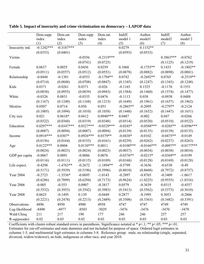
  31

Table 5. Impact of insecurity and crime victimization on democracy – LAPOP data Dem.supp.

index (1)

Dem.sat. index (2)

Dem.suppindex (3)

Dem.sat. index (4)

Indiff. model 1 (5)

Author. model1 (6)

Indiff. model2 (7)

Author. model 2 (8)

Insecurity ind. -0.1242*** -0.3187*** 0.0279 0.1152** (0.0353) (0.0401) (0.0593) (0.0533) Victim -0.0556 -0.2319*** 0.3863*** -0.0762 (0.0741) (0.0725) (0.1125) (0.1219) Female 0.0637 0.0855 0.0436 0.0259 0.1068 -0.1755** 0.1433 -0.1802** (0.0511) (0.0557) (0.0512) (0.0551) (0.0878) (0.0882) (0.0898) (0.0881) Relationship -0.0448 -0.1381 -0.0553 -0.1794** 0.0742 -0.2692** 0.0765 -0.2519** (0.0714) (0.0848) (0.0708) (0.0847) (0.1345) (0.1247) (0.1343) (0.1248) Kids 0.0371 -0.0261 0.0371 -0.026 -0.1165 0.1525 -0.1176 0.1551 (0.0838) (0.0955) (0.0839) (0.0943) (0.1584) (0.1460) (0.1574) (0.1477) White -0.0326 0.0831 -0.0335 0.0476 -0.1113 0.038 -0.0938 0.0488 (0.1167) (0.1249) (0.1168) (0.1215) (0.1649) (0.1961) (0.1657) (0.1962) Mestizo 0.0507 0.0714 0.056 0.051 -0.2865** -0.2095 -0.2797* -0.2124 (0.1005) (0.1094) (0.1010) (0.1058) (0.1448) (0.1652) (0.1447) (0.1651) City size 0.021 0.0618* 0.0412 0.0940*** 0.0487 -0.002 0.047 -0.0266 (0.0322) (0.0360) (0.0319) (0.0348) (0.0514) (0.0520) (0.0510) (0.0522) Education 0.0297*** -0.0347*** 0.0327*** -0.0329*** -0.0245* -0.0588*** -0.0285** -0.0596*** (0.0087) (0.0094) (0.0087) (0.0094) (0.0139) (0.0135) (0.0139) (0.0135) Income 0.0918*** 0.0307* 0.0926*** 0.0379** -0.0438* -0.0102 -0.0475** -0.0149 (0.0156) (0.0164) (0.0155) (0.0161) (0.0239) (0.0262) (0.0237) (0.0263) Age 0.0122*** 0.0004 0.0130*** 0.0011 -0.0100*** -0.0166*** -0.0097** -0.0177*** (0.0024) (0.0023) (0.0024) (0.0023) (0.0037) (0.0034) (0.0038) (0.0034) GDP per capita -0.0067 0.0091 -0.0086 0.0076 -0.0376** -0.0215* -0.0369** -0.0199 (0.0116) (0.0111) (0.0115) (0.0109) (0.0168) (0.0128) (0.0169) (0.0128) Life expect. -0.4298 -1.4763** -0.2672 -1.1894** -0.5799 -0.3636 -0.6538 -0.49 (0.5171) (0.5939) (0.5196) (0.5996) (0.8010) (0.8668) (0.7972) (0.8757) Year 2004 -0.2723 -1.3536* -0.0695 -1.0143 -0.2897 -0.8765 -0.3409 -1.0617 (0.6286) (0.7099) (0.6294) (0.7173) (0.9624) (1.0225) (0.9555) (1.0316) Year 2006 -0.005 -0.553 0.0907 -0.3817 0.0579 -0.3639 0.0315 -0.4557 (0.3532) (0.3953) (0.3542) (0.3983) (0.5413) (0.5562) (0.5373) (0.5610) Year 2008 0.0625 -0.1495 0.139 -0.0449 0.2877 -0.1995 0.3053 -0.2806 (0.2221) (0.2478) (0.2213) (0.2489) (0.3508) (0.3363) (0.3482) (0.3391) Observations 4896 4950 4900 4958 4747 4747 4749 4749 Log-likelihood -8490 -4977 -8503 -5029 -3476 -3476 -3470 -3470 Wald Chisq 211 217 190 177 246 246 257 257 R-sq(pseudo) 0.02 0.03 0.02 0.03 0.03 0.03 0.03 0.03 Coefficients with cluster-robust standard errors in parenthesis. Significance notated at * p<.1; ** p<.05; *** p<.01. Estimates for cut-off estimates and state dummies and not included for purpose of space. Ordered logit estimates in columns 1-5, and multinomial logit estimates in columns 5-8. Reference group: male, no relationship (single, separated, divorced, widow/widower), no kids, indigenous or other race, and year 2010.

  32

Table 6. Impact of insecurity on trust on institutions – LAPOP data

Political system (1)

Electoral system (2)

Congress (3)

Govern-ment (4)

Courts system (5)

Judicial system (6)

Police (7)

Army (8)

Insec. index -0.1082*** -0.1843*** -0.2225*** -0.2434*** -0.2192*** -0.3146*** -0.3371*** -0.2088*** (0.0383) (0.0360) (0.0330) (0.0346) (0.0323) (0.0361) (0.0347) (0.0345) Female 0.1168** 0.0295 -0.0232 0.0714 -0.0466 0.0364 0.0887* -0.2689*** (0.0525) (0.0522) (0.0533) (0.0497) (0.0542) (0.0510) (0.0484) (0.0540) Relationship -0.0075 0.1028 -0.1007 -0.0406 0.0648 0.0249 -0.0471 -0.0548 (0.0729) (0.0771) (0.0690) (0.0693) (0.0748) (0.0713) (0.0710) (0.0738) Kids 0.0221 -0.1204 0.1856** 0.0765 -0.1446* 0.0292 0.1029 0.1597* (0.0891) (0.0837) (0.0788) (0.0817) (0.0856) (0.0829) (0.0824) (0.0908) White 0.0618 0.1423 0.1696 0.1762 0.2792** 0.2195* 0.1851 -0.1575 (0.1093) (0.1122) (0.1211) (0.1258) (0.1149) (0.1277) (0.1244) (0.1192) Mestizo -0.0611 0.0686 0.1962* 0.0935 0.0483 0.1534 0.1247 -0.1121 (0.0878) (0.0966) (0.1064) (0.1088) (0.0923) (0.1055) (0.1011) (0.0990) City size 0.0713* 0.0475 0.0293 0.0761** 0.0316 0.044 0.1056*** -0.0108 (0.0368) (0.0312) (0.0296) (0.0321) (0.0331) (0.0375) (0.0397) (0.0307) Education 0.013 -0.0192** -0.0169* -0.0204** -0.0264*** -0.0075 -0.0111 -0.0069 (0.0086) (0.0085) (0.0086) (0.0086) (0.0088) (0.0087) (0.0085) (0.0087) Income -0.0321** 0.0122 0.011 -0.0093 0.0276* -0.0138 0.0002 0.0121 (0.0149) (0.0154) (0.0152) (0.0145) (0.0153) (0.0150) (0.0157) (0.0146) Age 0.0076*** -0.0082*** -0.0052** 0.0013 -0.0013 0.0002 -0.0018 -0.0025 (0.0023) (0.0022) (0.0023) (0.0023) (0.0024) (0.0023) (0.0022) (0.0022) GDP per cap. -0.0017 -0.0275*** -0.0026 -0.0083 -0.0015 -0.0017 0.0034 -0.0307*** (0.0087) (0.0093) (0.0084) (0.0082) (0.0093) (0.0084) (0.0104) (0.0079) Life expect. -0.2105 -1.1596** -0.483 -1.1779** -1.3859*** -0.6109 -1.0180* -1.2328*** (0.4895) (0.5125) (0.4490) (0.4924) (0.5170) (0.4955) (0.5671) (0.4358) Year 2004 -0.4918 -1.5007** -0.77 -1.7254*** -1.2476** -0.6392 -0.8942 -1.7821*** (0.5824) (0.6371) (0.5368) (0.5833) (0.6363) (0.5928) (0.6861) (0.5205) Year 2006 0.0978 0.1365 0.1353 -0.5767* -0.4537 -0.1926 -0.6087 -0.4664 (0.3177) (0.3479) (0.2931) (0.3296) (0.3445) (0.3305) (0.3740) (0.2909) Year 2008 -0.1125 0.1233 -0.0792 -0.3213 -0.2568 -0.1002 0.0194 -0.1925 (0.2041) (0.2237) (0.1950) (0.2212) (0.2170) (0.2296) (0.2397) (0.1961) Observations 5016 5030 4856 5015 4786 5043 5075 4998 Log-lik. -8936 -9278 -8924 -9192 -8782 -9307 -9276 -8480 Wald Chi sq 203.2 288.1 247.6 284.4 272.3 257.5 351.5 224.2 R-sq(pseudo) 0.02 0.02 0.02 0.02 0.02 0.02 0.03 0.02 Ordered logit coefficients with cluster-robust standard errors in parenthesis. Significance notated at * p<.1; ** p<.05; *** p<.01. Estimates for cut-off estimates and state dummies and not included for purpose of space. Reference group: male, no relationship (single, separated, divorced, widow/widower), no kids, indigenous or other race, and year 2010.

  33

Table 7. Impact of crime victimization on trust on institutions – LAPOP data Political

system (1)

Electoral system (2)

Congress (3)

Govern-ment (4)

Courts system (5)

Judicial system (6)

Police (7)

Army (8)

Victim -0.2314*** -0.2709*** -0.2369*** -0.2110*** -0.3143*** -0.4259*** -0.3160*** -0.1803*** (0.0690) (0.0655) (0.0624) (0.0695) (0.0707) (0.0642) (0.0658) (0.0671) Female 0.0862 -0.0128 -0.0672 0.0258 -0.0998* -0.0275 0.0288 -0.3027*** (0.0526) (0.0519) (0.0535) (0.0497) (0.0539) (0.0507) (0.0486) (0.0542) Relationship -0.0346 0.0757 -0.1211* -0.0706 0.0316 -0.0221 -0.0958 -0.0815 (0.0730) (0.0772) (0.0686) (0.0694) (0.0750) (0.0720) (0.0726) (0.0738) Kids 0.0338 -0.1132 0.1803** 0.0709 -0.1459* 0.0384 0.1162 0.1545* (0.0888) (0.0844) (0.0779) (0.0815) (0.0850) (0.0847) (0.0844) (0.0912) White 0.0578 0.1274 0.1373 0.1617 0.2562** 0.1922 0.1694 -0.1586 (0.1090) (0.1121) (0.1201) (0.1255) (0.1163) (0.1296) (0.1262) (0.1204) Mestizo -0.0596 0.0596 0.1785* 0.0836 0.0386 0.1399 0.1198 -0.1052 (0.0880) (0.0973) (0.1049) (0.1076) (0.0923) (0.1071) (0.1008) (0.0992) City size 0.0817** 0.0630** 0.0514* 0.1029*** 0.0513 0.0737* 0.1384*** 0.0126 (0.0361) (0.0313) (0.0302) (0.0323) (0.0335) (0.0377) (0.0402) (0.0310) Education 0.0150* -0.0172** -0.0136 -0.0185** -0.0230** -0.0028 -0.0073 -0.0039 (0.0085) (0.0085) (0.0086) (0.0087) (0.0089) (0.0088) (0.0084) (0.0087) Income -0.0293** 0.0181 0.0135 -0.005 0.0323** -0.007 0.0077 0.0146 (0.0147) (0.0151) (0.0150) (0.0143) (0.0153) (0.0149) (0.0157) (0.0145) Age 0.0076*** -0.0080*** -0.0044** 0.0021 -0.0007 0.0009 -0.0009 -0.0015 (0.0023) (0.0022) (0.0022) (0.0023) (0.0024) (0.0023) (0.0022) (0.0022) GDP per cap. -0.0026 -0.0294*** -0.0043 -0.0096 -0.0038 -0.0041 0.0011 -0.0313*** (0.0088) (0.0092) (0.0084) (0.0082) (0.0095) (0.0085) (0.0106) (0.0079) Life expect. -0.0359 -0.9946** -0.2946 -0.9796** -1.1526** -0.3405 -0.658 -0.9508** (0.4968) (0.5049) (0.4558) (0.4937) (0.5185) (0.4998) (0.5637) (0.4378) Year 2004 -0.2985 -1.3005** -0.5408 -1.4751** -0.9832 -0.3414 -0.4653 -1.4459*** (0.5896) (0.6227) (0.5433) (0.5831) (0.6372) (0.5944) (0.6807) (0.5220) Year 2006 0.2084 0.2366 0.234 -0.4531 -0.3149 -0.0426 -0.3993 -0.3166 (0.3225) (0.3422) (0.2997) (0.3323) (0.3468) (0.3353) (0.3744) (0.2935) Year 2008 -0.0576 0.1894 0.0038 -0.2376 -0.1821 -0.0098 0.1581 -0.0929 (0.2059) (0.2194) (0.1995) (0.2215) (0.2176) (0.2307) (0.2408) (0.1967) Observations 5022 5035 4865 5024 4794 5051 5083 5002 Log-lik. -8950 -9298 -8964 -9233 -8811 -9362 -9342 -8519 Wald Chi sq 209.6 284.1 219.4 249.2 245.3 229.3 267.2 195.4 R-sq(pseudo) 0.02 0.02 0.01 0.02 0.02 0.02 0.02 0.01 Ordered logit coefficients with cluster-robust standard errors in parenthesis. Significance notated at * p<.1; ** p<.05; *** p<.01. Estimates for cut-off estimates and state dummies and not included for purpose of space. Reference group: male, no relationship (single, separated, divorced, widow/widower), no kids, indigenous or other race, and year 2010.

  34

Table 8. Impact of insecurity on trust in institutions – ENSI data Local pol Transit pol. State pol AFI Fed pol prev Fed police Public minist Army Pol parties (1) (2) (3) (4) (5) (6) (7) (8) (9) Insecurity index -0.6714*** -0.5624*** -0.5415*** -0.3731*** -0.4357*** -0.4380*** -0.5718*** -0.2771*** -0.4995*** (0.0208) (0.0215) (0.0270) (0.0335) (0.0268) (0.0201) (0.0203) (0.0204) (0.0206) Urban -0.4638*** -0.2609*** -0.3270*** -0.2590*** -0.1894*** -0.1102*** -0.2215*** -0.0296 -0.1844*** (0.0296) (0.0304) (0.0372) (0.0487) (0.0375) (0.0303) (0.0301) (0.0310) (0.0306) Female 0.0269 0.0686*** 0.0253 -0.1353*** -0.2028*** -0.1636*** 0.0076 -0.3114*** 0.005 (0.0224) (0.0233) (0.0306) (0.0500) (0.0406) (0.0224) (0.0222) (0.0252) (0.0252) Age -0.0033 -0.0057* -0.0343*** -0.0349*** -0.0255*** -0.0208*** -0.0219*** 0.004 -0.0122*** (0.0031) (0.0034) (0.0044) (0.0057) (0.0045) (0.0029) (0.0029) (0.0029) (0.0030) Age squared 0.0001*** 0.0001*** 0.0003*** 0.0002*** 0.0002*** 0.0002*** 0.0002*** -0.0001* 0.0001*** 0.0000 (0.0000) (0.0000) (0.0001) (0.0001) (0.0000)   (0.0000)   (0.0000)   (0.0000)  Primary -0.1627*** -0.0969** -0.2490*** -0.2062** -0.0525 0.052 0.0946** 0.0289 -0.0454 (0.0382) (0.0418) (0.0613) (0.0920) (0.0569) (0.0380) (0.0407) (0.0386) (0.0400) Sec and high -0.1990*** -0.2026*** -0.4718*** -0.2521*** -0.062 0.0789* 0.0329 0.1532*** -0.0946** (0.0399) (0.0439) (0.0621) (0.0947) (0.0591) (0.0403) (0.0422) (0.0407) (0.0426) More than high -0.2442*** -0.2585*** -0.6757*** -0.4154*** -0.1890*** 0.1199*** 0.0153 0.2262*** -0.0589 (0.0398) (0.0428) (0.0618) (0.0897) (0.0541) (0.0390) (0.0416) (0.0391) (0.0410) Work -0.0577** -0.0433* -0.0523 -0.1030* -0.0583 -0.0137 0.0071 -0.0712*** -0.0024 (0.0241) (0.0250) (0.0328) (0.0536) (0.0433) (0.0236) (0.0230) (0.0270) (0.0275) No work -0.1965*** -0.0783 -0.0739 -0.0943 -0.0425 -0.0165 -0.0549 -0.0359 -0.0023 (0.0526) (0.0546) (0.0799) (0.0985) (0.0740) (0.0487) (0.0513) (0.0508) (0.0524) GDP per capita 0.0018 0.0046*** 0.0002 0.0023 0.0035 0.0031 0.0032 -0.0086*** 0.0111*** (0.0016) (0.0018) (0.0021) (0.0031) (0.0022) (0.0026) (0.0027) (0.0028) (0.0030) Life expect. 0.6462*** 0.9910*** 1.0411*** 0.2987 0.7772*** 0.1496 0.341 -1.9825** -1.1413 (0.1695) (0.1712) (0.2161) (0.2842) (0.2354) (0.8597) (0.8955) (0.9331) (1.0216) Year 2004 0.9880*** 1.1382*** 0.8247*** 0.9688*** 1.4073*** (0.1710) (0.1716) (0.2112) (0.2788) (0.2297) Year 2007 0.3704*** 0.2597*** 0.1752** 0.3002*** 0.3302*** 0.2812 -0.0876 -0.5740** -0.5343* (0.0597) (0.0601) (0.0741) (0.0959) (0.0836) (0.2626) (0.2726) (0.2863) (0.3084) Year 2008 0.2508*** 0.0770** 0.068 0.2473*** 0.2081*** 0.1714 -0.1184 0.0258 -0.4009** (0.0374) (0.0369) (0.0496) (0.0620) (0.0501) (0.1363) (0.1409) (0.1467) (0.1616) Observations 148000 139460 84659 55431 83426 129371 127212 131749 134916 F value 75.66 77.53 46.51 22.85 42.7 54.77 66.35 63.49 42.74 Coefficients with standard errors in parenthesis. Significance notated at * p<.1; ** p<.05; *** p<.01. Estimates for state dummies not included for purpose of space. Ordered logit estimates considering clusters and weights (no stratification; svy Stata command). Reference group: no education, not in labor force, and year 2009.

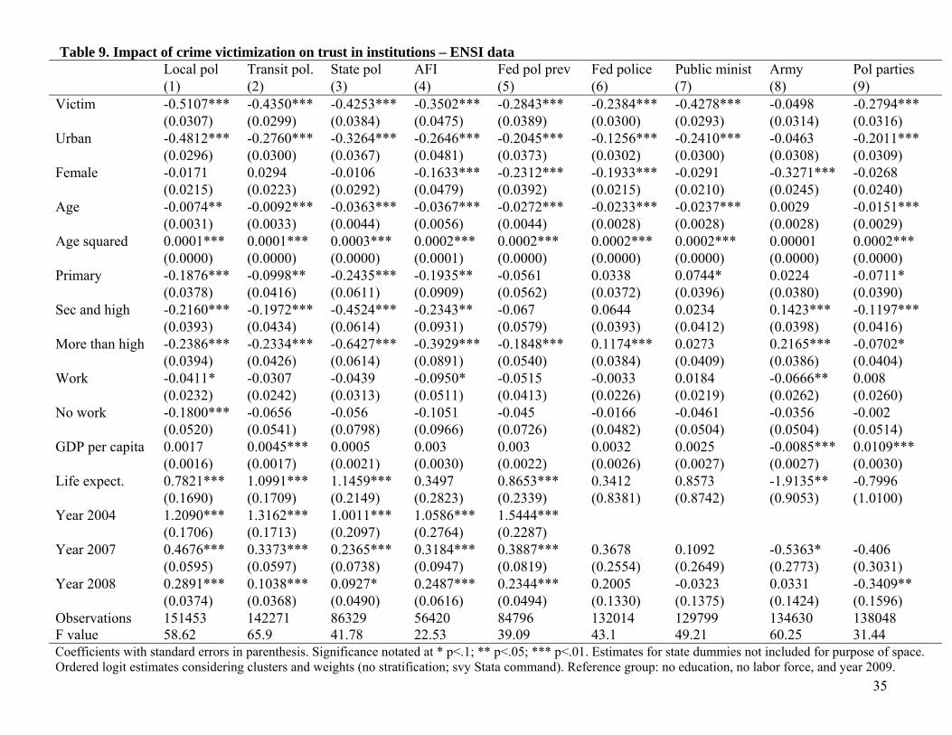
  35

Table 9. Impact of crime victimization on trust in institutions – ENSI data Local pol Transit pol. State pol AFI Fed pol prev Fed police Public minist Army Pol parties (1) (2) (3) (4) (5) (6) (7) (8) (9) Victim -0.5107*** -0.4350*** -0.4253*** -0.3502*** -0.2843*** -0.2384*** -0.4278*** -0.0498 -0.2794*** (0.0307) (0.0299) (0.0384) (0.0475) (0.0389) (0.0300) (0.0293) (0.0314) (0.0316) Urban -0.4812*** -0.2760*** -0.3264*** -0.2646*** -0.2045*** -0.1256*** -0.2410*** -0.0463 -0.2011*** (0.0296) (0.0300) (0.0367) (0.0481) (0.0373) (0.0302) (0.0300) (0.0308) (0.0309) Female -0.0171 0.0294 -0.0106 -0.1633*** -0.2312*** -0.1933*** -0.0291 -0.3271*** -0.0268 (0.0215) (0.0223) (0.0292) (0.0479) (0.0392) (0.0215) (0.0210) (0.0245) (0.0240) Age -0.0074** -0.0092*** -0.0363*** -0.0367*** -0.0272*** -0.0233*** -0.0237*** 0.0029 -0.0151*** (0.0031) (0.0033) (0.0044) (0.0056) (0.0044) (0.0028) (0.0028) (0.0028) (0.0029) Age squared 0.0001*** 0.0001*** 0.0003*** 0.0002*** 0.0002*** 0.0002*** 0.0002*** 0.00001 0.0002*** (0.0000) (0.0000)   (0.0000)   (0.0001) (0.0000)   (0.0000)   (0.0000)   (0.0000)   (0.0000)  Primary -0.1876*** -0.0998** -0.2435*** -0.1935** -0.0561 0.0338 0.0744* 0.0224 -0.0711* (0.0378) (0.0416) (0.0611) (0.0909) (0.0562) (0.0372) (0.0396) (0.0380) (0.0390) Sec and high -0.2160*** -0.1972*** -0.4524*** -0.2343** -0.067 0.0644 0.0234 0.1423*** -0.1197*** (0.0393) (0.0434) (0.0614) (0.0931) (0.0579) (0.0393) (0.0412) (0.0398) (0.0416) More than high -0.2386*** -0.2334*** -0.6427*** -0.3929*** -0.1848*** 0.1174*** 0.0273 0.2165*** -0.0702* (0.0394) (0.0426) (0.0614) (0.0891) (0.0540) (0.0384) (0.0409) (0.0386) (0.0404) Work -0.0411* -0.0307 -0.0439 -0.0950* -0.0515 -0.0033 0.0184 -0.0666** 0.008 (0.0232) (0.0242) (0.0313) (0.0511) (0.0413) (0.0226) (0.0219) (0.0262) (0.0260) No work -0.1800*** -0.0656 -0.056 -0.1051 -0.045 -0.0166 -0.0461 -0.0356 -0.002 (0.0520) (0.0541) (0.0798) (0.0966) (0.0726) (0.0482) (0.0504) (0.0504) (0.0514) GDP per capita 0.0017 0.0045*** 0.0005 0.003 0.003 0.0032 0.0025 -0.0085*** 0.0109*** (0.0016) (0.0017) (0.0021) (0.0030) (0.0022) (0.0026) (0.0027) (0.0027) (0.0030) Life expect. 0.7821*** 1.0991*** 1.1459*** 0.3497 0.8653*** 0.3412 0.8573 -1.9135** -0.7996 (0.1690) (0.1709) (0.2149) (0.2823) (0.2339) (0.8381) (0.8742) (0.9053) (1.0100) Year 2004 1.2090*** 1.3162*** 1.0011*** 1.0586*** 1.5444*** (0.1706) (0.1713) (0.2097) (0.2764) (0.2287) Year 2007 0.4676*** 0.3373*** 0.2365*** 0.3184*** 0.3887*** 0.3678 0.1092 -0.5363* -0.406 (0.0595) (0.0597) (0.0738) (0.0947) (0.0819) (0.2554) (0.2649) (0.2773) (0.3031) Year 2008 0.2891*** 0.1038*** 0.0927* 0.2487*** 0.2344*** 0.2005 -0.0323 0.0331 -0.3409** (0.0374) (0.0368) (0.0490) (0.0616) (0.0494) (0.1330) (0.1375) (0.1424) (0.1596) Observations 151453 142271 86329 56420 84796 132014 129799 134630 138048 F value 58.62 65.9 41.78 22.53 39.09 43.1 49.21 60.25 31.44 Coefficients with standard errors in parenthesis. Significance notated at * p<.1; ** p<.05; *** p<.01. Estimates for state dummies not included for purpose of space. Ordered logit estimates considering clusters and weights (no stratification; svy Stata command). Reference group: no education, no labor force, and year 2009.

  36

Table 10. Impact of insecurity on trust in institutions, regional and time variation (distance to border and narco density) ENSI data

Local pol State pol Fed pol prev Local pol State pol Fed pol prev (1) (2) (3) (4) (5) (6) Insecurity ind. -0.6714*** -0.5415*** -0.4357*** -0.6714*** -0.5415*** -0.4357*** (0.0208) (0.0270) (0.0268) (0.0208) (0.0270) (0.0268) Dist. border 0.0015*** 0.0008*** 0.0007** (0.0002) (0.0003) (0.0003) Narco density -0.0989*** -0.0525*** -0.0435** (0.0163) (0.0202) (0.0212) Year 2004 0.9880*** 0.8247*** 1.4073*** 0.9880*** 0.8247*** 1.4073*** (0.1710) (0.2112) (0.2297) (0.1710) (0.2112) (0.2297) Year 2007 0.3704*** 0.1752** 0.3302*** 0.3704*** 0.1752** 0.3302*** (0.0597) (0.0741) (0.0836) (0.0597) (0.0741) (0.0836) Year 2008 0.2508*** 0.068 0.2081*** 0.2508*** 0.068 0.2081*** (0.0374) (0.0496) (0.0501) (0.0374) (0.0496) (0.0501) Observations 148000 84659 83426 148000 84659 83426 Population 1.94E+08 1.13E+08 1.13E+08 1.94E+08 1.13E+08 1.13E+08 F value 75.66 46.51 42.7 75.66 46.51 42.7 Coefficients with standard errors in parenthesis. Significance notated at * p<.1; ** p<.05; *** p<.01. Estimates for control variables (urban, female, age, age squared, primary, sec and high, more than high, work, no work, GDP per capita, and life expectancy) and state dummies not included for purpose of space. Ordered logit estimates considering clusters and weights (no stratification; svy Stata command). Reference group: no education, no labor force, and year 2009.

  37

Table 11. Impact of insecurity on trust in institutions, regional and time variation (marihuana, region, and time trend) ENSI data

Local pol State pol Fed pol prev Local pol State pol Fed pol prev (1) (2) (4) (6) (7) (9) Insecurity ind. -0.6699*** -0.5413*** -0.4333*** -0.6681*** -0.5405*** -0.4357*** (0.0208) (0.0270) (0.0268) (0.0207) (0.0270) (0.0267) Marihuana 0.0630*** 0.023 0.1444*** (0.0171) (0.0214) (0.0216) Noreste 0.0438 0.3438** -0.0904 (0.1384) (0.1592) (0.1687) Noroeste 0.2998*** 0.1852 -0.1826 (0.1061) (0.1309) (0.1334) Year trend -0.0781*** 0.042 0.0465 (0.0285) (0.0356) (0.0393) Noreste*year trend -0.1264*** -0.1421*** -0.1029*** (0.0296) (0.0337) (0.0354) Noroeste*year trend -0.0455** -0.0669** -0.1416*** (0.0201) (0.0268) (0.0264) Year 2004 1.0513*** 0.8567*** 1.6006*** (0.1733) (0.2138) (0.2317) Year 2007 0.3811*** 0.1824** 0.3682*** (0.0599) (0.0745) (0.0836) Year 2008 0.2485*** 0.0696 0.2098*** (0.0373) (0.0496) (0.0499) Observations 148000 84659 83426 148000 84659 83426 Population 1.9E+08 1.1E+08 1.1E+08 1.9E+08 1.1E+08 1.1E+08 F value 74.2 45.55 44.88 76.06 46.33 42.83 Coefficients with standard errors in parenthesis. Significance notated at * p<.1; ** p<.05; *** p<.01. Estimates for control variables (urban, female, age, age squared, primary, sec and high, more than high, work, no work, GDP per capita, and life expectancy) and state dummies not included for purpose of space. Ordered logit estimates considering clusters and weights (no stratification; svy Stata command). Reference group: no education, no labor force, and year 2009.

  38

Table 12. Marginal effect of insecurity and crime victimization on satisfaction with democracy and trust in the police dy/dx            Satisfaction with democracy Pr(y=1) Pr(y=2) Pr(y=3) Pr(y=4) Insecurity index (T5, C2) 0.0235 0.0513 -0.0642 -0.0106 Victim dummy (T5, C4) 0.0173 0.038 -0.0476 -0.0077   Trust on local police Pr(y=1) Pr(y=2) Pr(y=3) Insecurity index (T8, C1) 0.1104 -0.0233 -0.0871 Victim dummy (T9, C1) 0.0844 -0.0168 -0.0677

Table 13. Adding average of satisfaction with democracy and trust in the local police at the state level in previous year

Dependent variable Satisfaction with democracy Trust local police

(1) (2) (3) (4) Insecurity index -0.2921*** -0.6178***

(0.0470) (0.0252) Victim dummy -0.2269*** -0.4993***

(0.0819) (0.0359) Avg. Democ. Satis. Lag -0.8894*** -0.8480***

(0.3207) (0.3168) Avg. Trust Local Pol. Lag -0.2265 -0.1952 (0.2969) (0.3032) Observations 3,630 3,642 101,204 103,404 Coefficients with standard errors in parenthesis. Significance notated at * p<.1; ** p<.05; *** p<.01. Estimates in columns 1 and 2 are the same as those shown in Table 5, columns 2 and 4, with additional variable. Estimates in columns 3 and 4 are the same as those shown in Tables 8 and 9, column 1, with additional variable.

The Political Economy of Health Worker Absence: Experimental

Evidence from Pakistan∗

Michael Callen† Saad Gulzar‡

Ali Hasanain§ Yasir Khan¶

First Version:January 22, 2013

Prelimary. Not for Circulation

Abstract

In many developing countries, public sector absence is both common and highlyintractable. One explanation for this is that politicians provide public jobs with limitedwork requirements as patronage. We test this explanation for absence in Pakistanusing: (i) a controlled evaluation of a novel smartphone technology designed to increaseinspections at rural clinics; (ii) data on election outcomes in the 241 constituencieswhere the experiment took place; (iii) attendance recorded during unannounced visitsand; (iv) surveys of connections between local politicians and health staff. Threeresults suggest that absence is linked to patronage. First, while doctors are presentat 40 percent of facilities during unannounced visits in highly competitive electoraldistricts, they are almost always absent in captured districts. Second, doctors whoknow their local parliamentarian personally are present during an average of 0.727of 3 unannounced visits, while unconnected doctors are present at 1.237 of the threevisits. Last, the effects of the smartphone monitoring technology, which almost doubledinspection rates, are highly localized to competitive electoral districts.

∗Authors’ Note: We thank Farasat Iqbal (Punjab Health Sector Reforms Project) for championing andimplementing the project and, Asim Fayaz, and Zubair Bhatti (World Bank) for designing the program.Support is provided by the International Growth Centre (IGC) political economy program and the IGCPakistan Country Office. We thank Eli Berman, Ali Cheema, Naved Hamid, Gordon Hanson, Asim Khwaja,Craig McIntosh, Ijaz Nabi, Christopher Woodruff and seminar participants at DFID, UC San Diego, andGrowth Week at LSE for insightful comments. Excellent research assistance was provided by MuhammadZia Mehmood, Haseeb Ali, and Arman Rezaee. We thank Ali Cheema and Farooq Naseer for kindly sharingtheir data on election outcomes.†University of California, Los Angeles. email: mjcallen@ucsd.edu‡New York University§Lahore University of Management Sciences¶International Growth Centre - Pakistan

1

1 Introduction

Patronage politics often leads to the selection of inefficient policies. In clientelistic systems,

politicians win office by providing targeted benefits to supporters at the cost of services which

provide broader collective benefits, with negative implications for economic and human de-

velopment.1 Government jobs are commonly used for patronage. In developing countries,

government workers are also frequently absent despite being generally well-compensated.2

Moreover, public sector absence also tends to be intractable. Many policies aimed at im-

proving attendance only work temporarily. We investigate whether the persistence of public

sector absence in developing countries is linked to the use of public jobs as patronage.

Governments jobs are ideal for patronage; they can be targeted to individuals, provide a

credible stream of benefits, and are reversible (Robinson and Verdier 2002). This is partic-

ularly true if politicians can minimize the actual work required in the position. Historically,

jobs have been used as patronage in many settings. Chubb (1983) argues that, under the

control of the Christian Democrats in Naples and Palermo during the 1950s, politicians al-

located public sector jobs “on the basis of political favoritism, often having nothing to do

with effective work loads or even with the actual presence of the employee in his office.” So-

rauf (1956) describes a similar system for road workers in Centre County, Pennsylvania and

Johnston (1979) for unskilled public sector jobs in New Haven, Connecticut. Wilson (1961)

describes the centrality of public jobs in maintaining the Tammany Hall political machine

in New York and the Democratic Party machine in Chicago in the early 20th century. In all

three settings, the beneficiaries commonly rewarded politicians with votes, party campaign

1Bates (1981) provides the authoritative account relating to Africa’s development, arguing that Africangovernments deliberately overvalued their exchange rates in order to subsidize politically powerful urbanelites with cheaper imports at the expense of the rural poor. Khwaja and Mian (2005) and Fisman (2001)provide evidence that politicians provide preferential government benefits to firms and Dube et al. (2011) findpatterns in stock returns consistent with the U.S. government providing insider information to investors aboutfuture international interventions. Dahlberg and Johansson (2002) show that the Swedish central governmentallocated discretionary government grants for ecologically sustainable development based primarily on thenumber of swing voters.

2We find that 68.5 percent of doctors are absent prior to our intervention. This compares with the averageacross Bangladesh, Ecuador, India, Indonesia, Peru and Uganda of 35 percent reported in Chaudhury et al.(2006).

2

work, monetary contributions, and by swinging blocs of voters.3

The development literature identifies public worker absence as key obstacle to delivering

services to the poor (Banerjee and Duflo 2006; Chaudhury et al. 2006). With the notable

exception of a camera monitoring initiative in Udaipur, Rajasthan reported in Duflo et al.

(2012), absence appears unresponsive to increasing inspections, particularly when inspectors

are not assisted by technologies that limit their discretion. Banerjee and Duflo (2006) review

unsuccessful monitoring initiatives in Kenya and India and Banerjee et al. (2008) details the

complicity of the local health administration in the failure of a monitoring initiative in rural

Rajasthan. These findings support the broader position that the effects anti-corruption

initiatives tend to attenuate over time (Olken and Pande 2012).

These studies propose several solutions. Duflo et al. (2012) indicate that teachers must

also receive a premium for attending work; monitoring fails when workers are not paid more

than their outside wage. Banerjee et al. (2008) encourage increasing senior level ownership

and improving incentives for senior managers to make sure their subordinates are present.

Chaudhury et al. (2006) explore the possibility of local monitoring, acknowledging that

decentralized management systems may be more prone to local capture. We investigate

whether public worker absence is linked to the usefulness of jobs with minimal attendance

requirements for political patronage.

We examine this in three ways. First, we combine data on election outcomes in local

elections with independently collected data on doctor absence. Second, we directly inter-

view doctors to examine whether their connections to politicians are related to their job

performance and to the desirability of their posting. Last, we experimentally evaluate a

novel smartphone attendance monitoring program across 241 of the 297 (81 percent) of the

Provincial Assembly constituencies in Punjab, examining whether impact depends on the

degree of local political competition.4

3Sorauf (1956) shows that the road crew organizers were more politically active than their subordinates,arguing that the strongest supporters should be placed in jobs where they have the most influence.

4There are 371 seats in the Punjab Provincial Assembly. Of these, 66 are reserved for women and eightare reserved for non-muslims, leaving 297 elected seats.

3

This investigation yields three main results which link health service provision to local

political outcomes. First, absence is more severe in less competitive districts. Second, polit-

ically connected doctors appear able to obtain better postings. Third, while the smartphone

monitoring program almost doubled health worker attendance, the effects of the program

are highly localized to competitive districts.

We point to two central implications. First, our data link the finding in development

economics that absence is both severe and difficult to address to the observation in political

science that public jobs represent a core means of patronage. Second, remedying the problem

of absence faces the challenge of well-protected government jobs being an attractive means

of patronage, both for politicians and constituents. This suggests that lasting improvements

to health worker attendance may require strictly limiting the ability of elected politicians to

interfere in the allocation of public sector jobs. Additionally, policies which reduce politicians

reliance on patronage may address the problem of absence.

The paper proceeds as follows: Section 2 provides institutional details of the public

health sector and describes the smartphone monitoring technology. Section 3 describes the

experimental evaluation. Section 4 reviews the primary data on absence. Section 5 presents

our non-experimental analysis of election outcomes and doctor absence. Section 6 provides

results from the experiment and Section 7 concludes.

2 Background

2.1 The Public Health System

In Punjab province, the provision of health care services is managed by the Department of

Health, which is based at the provincial headquarters in Lahore. There are five major types

of facilities: (1) Basic Health Unit (BHU); (2) Rural Health Center (RHC); (3) Tehsil Head-

quarter Hospital5 (THQ); (4) District Headquarter Hospital (DHQ); (5) Teaching Hospitals.

5In Punjab, a Tehsil is the largest sub-division of a district

4

We focus on Basic Health Units (BHUs). BHUs are the smallest public health care units.

They are designed to be the first stop for patients seeking medical treatment in govern-

ment facilities. (Hereafter in this paper, we use the word ’clinic’ interchangeably to describe

BHUs). There are 2496 BHUs in Punjab.6 They largely serve rural populations; almost all

such clinics are exclusively operating in rural and peri-urban areas. These clinics provide

several services, including out-patient services, neo-natal and reproductive healthcare, and

vaccinations against diseases. Each facility is headed by a doctor, known as the Medical Offi-

cer, who is supported by a Dispenser, a Lady Health Visitor, a School Health and Nutrition

Supervisor, a Health/Medical Technician, a Mid-wife and other ancillary staff. Officially,

clinics are open, and all staff are supposed to be present, from 8am to 2pm.

2.1.1 Health Sector Administration

District governments are responsible for managing local health facilities. The District Health

Department is headed by an Executive District Officer who reports both to the chief bu-

reaucrat of the district and to the most senior provincial health officials.7 He is supported

by several Deputy District Officers, typically one for each tehsil.8 Figure 1 depicts the

(simplified) health administration hierarchy in Punjab, Pakistan.

The central department has also established a parallel entity known as the Punjab Health

Sector Reform Program (PHSRP). PHSRP is tasked with initiating programs to reform the

primary health system with support from international and donor organizations. PHSRP is

responsible for the implementation of the smartphone monitoring program we evaluate in

this paper.

The Deputy District Officer is the lowest position in the officer-cadre of district health

administration. He inspects all health facilities in a given Tehsil. This officer is required

6Each Basic Health Unit serves approximately one Union Council (Union Councils are smallest adminis-trative units in Pakistan).

7The Director General of Health Services and the Secretary of the Health Department8The Executive District Officer is also supported by other staff, but they are excluded for clarity because

they are irrelevant to our discussion here.

5

Health  Secretary  

Execu/ve  District  Officer  (EDO)  

Deputy  District  Officer  (DDO)  

Medical  Officer    (MO)  

Figure 1: Health Sector Administration in Punjab

to visit every clinic at least once a month and record information collected during the visit

on a standard form. The Deputy District Officer has authority to punish the clinic’s absent

staff by issuing a show-cause notice, suspension and withholding pay (in case of contract

staff). The Executive District Officer relies entirely on this subordinate officer to ensure

staff presence. As the administrative head of the health department in the district, the

Executive District Officer desires smooth functioning of the setup at minimum acceptable

level. He relies on the Deputy District Officer to ensure this smooth function by sanctioning

underperforming facilities in terms of staff attendance, medicine availability and cleanliness

etc.

2.1.2 Career Concerns and Internal Agency Problems

The Executive District Officer faces a severe agency problem in managing his deputy inspec-

tors. This is for several reasons. First, he has limited visibility into the inspectors’ activities.

Second, he has only two weak means of sanctioning an inspector. He can either issue a

verbal reprimand or, in serious cases, send a written request for investigation to provincial

6

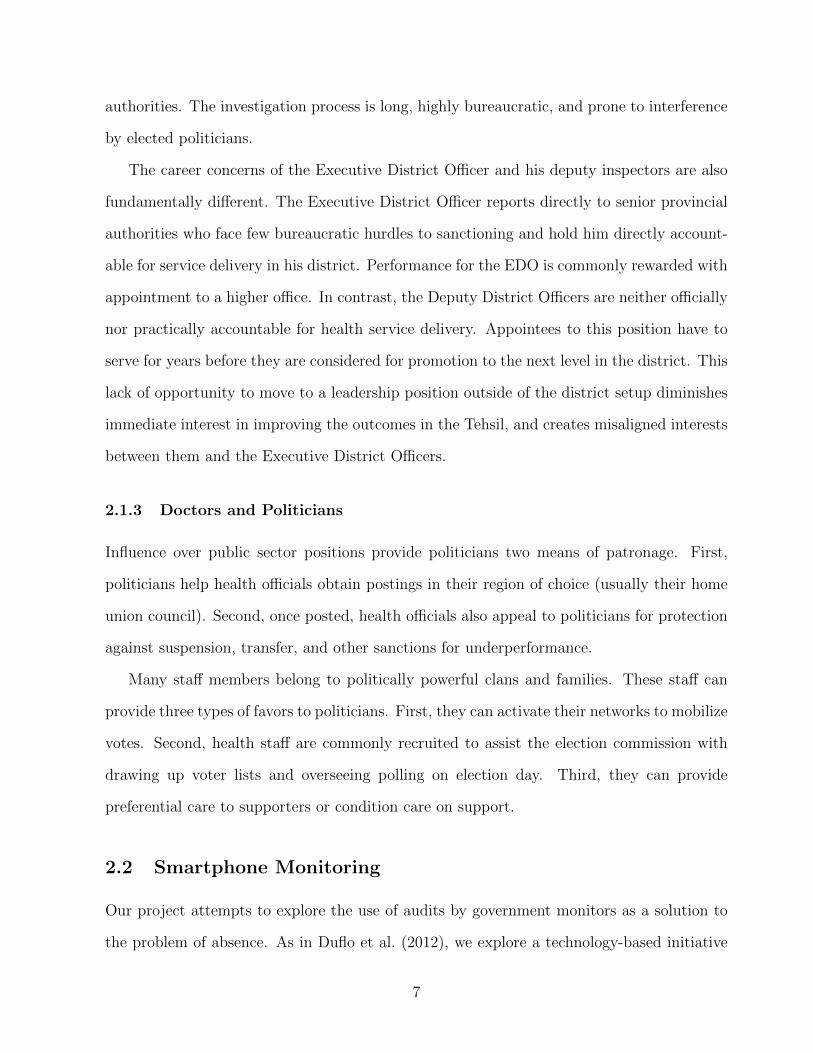
authorities. The investigation process is long, highly bureaucratic, and prone to interference

by elected politicians.

The career concerns of the Executive District Officer and his deputy inspectors are also

fundamentally different. The Executive District Officer reports directly to senior provincial

authorities who face few bureaucratic hurdles to sanctioning and hold him directly account-

able for service delivery in his district. Performance for the EDO is commonly rewarded with

appointment to a higher office. In contrast, the Deputy District Officers are neither officially

nor practically accountable for health service delivery. Appointees to this position have to

serve for years before they are considered for promotion to the next level in the district. This

lack of opportunity to move to a leadership position outside of the district setup diminishes

immediate interest in improving the outcomes in the Tehsil, and creates misaligned interests

between them and the Executive District Officers.

2.1.3 Doctors and Politicians

Influence over public sector positions provide politicians two means of patronage. First,

politicians help health officials obtain postings in their region of choice (usually their home

union council). Second, once posted, health officials also appeal to politicians for protection

against suspension, transfer, and other sanctions for underperformance.

Many staff members belong to politically powerful clans and families. These staff can

provide three types of favors to politicians. First, they can activate their networks to mobilize

votes. Second, health staff are commonly recruited to assist the election commission with

drawing up voter lists and overseeing polling on election day. Third, they can provide

preferential care to supporters or condition care on support.

2.2 Smartphone Monitoring

Our project attempts to explore the use of audits by government monitors as a solution to

the problem of absence. As in Duflo et al. (2012), we explore a technology-based initiative

7

that seeks, in part, to detect absence. There is increasing interest in using ICT to rapidly

collect information that is useful to auditors. Solving intra-bureaucracy agency problems

is a potential application. We implement a smartphone-based solution that allows health

system inspectors to upload the results of their assigned visit to a basic health facility to

an aggregating website (dashboard), which instantly updates reports at different levels of

aggregation (zonal and provincial) with the information captured by this most recent visit.

The “Monitoring the Monitors” program replaced the traditional paper-based monitoring

system, which collects data on facility utilization, resource availability, and worker absence,

with an android-based smartphone application. Data are transmitted to a central database

using a General Packet Radio Service (GPRS) in real time. Data are then aggregated and

summary statistics, charts, and graphs are presented in a format designed in collaboration

with senior health officials. That data are: (i) aggregated in the province in real time; (ii) geo-

tagged, time-stamped, and complemented with facility staff photos to check for reliability;

and (iii) available in real time to district and provincial officers through an online dashboard.

Figure 2 shows one view of the online dashboard.

Application development started in August 2011. After developing the application and

linking it to a beta version of the online dashboard, the system was piloted in the district

of Khanewal. We remove Khanewal district from the experimental sample. Health adminis-

tration staff were provided with smartphones and trained to use the application. The main

purpose of the pilot was to ensure that the technology was working and to refine the appli-

cation and the dashboard. During the pilot, several inspectors requested that the program

require pictures of all staff in attendance, not just the inspector because they thought it

might reduce pressure from health staff to falsify attendance.

8

Figure 2: Online Dashboard - Summary of Inspection Compliance by District

3 Experiment

Our experimental sample comprised all health facilities in the district of Punjab, which has

a population of 100 million. Tens of millions of public sector health users therefore stood to

benefit from the program. We randomly implemented the program in 18 of the 35 districts in

our experimental sample. In assigning treatment we stratified on baseline attendance (from

primary or secondary data) and the number of clinics in a district to ensure a roughly even

number of treatments and controls. Figure 3 depicts control and treatment districts.

We randomized at the district level. The intervention channels information about in-

spections to district health officials; randomization at a finer level is therefore very likely to

generate externalities. The Department of Health also determined that sub-district random-

ization was not administratively feasible. Cluster randomization also allays some concerns

about externalities generated by interactions between inspectors in the same district. All

9

Figure 3: Treatment and Control Districts

inspectors in a district are required to attend monthly meetings. While they typically have

frequent interactions within districts, these relations are much weaker across districts.

4 Data

We collected primary data on a representative sample of BHUs 850 (34 percent) of the 2,496

Basic Health Units in Punjab. We visited these facilities three times, first in November

2011, then in June 2012 and in October 2012. BHUs were selected randomly using an Equal

10

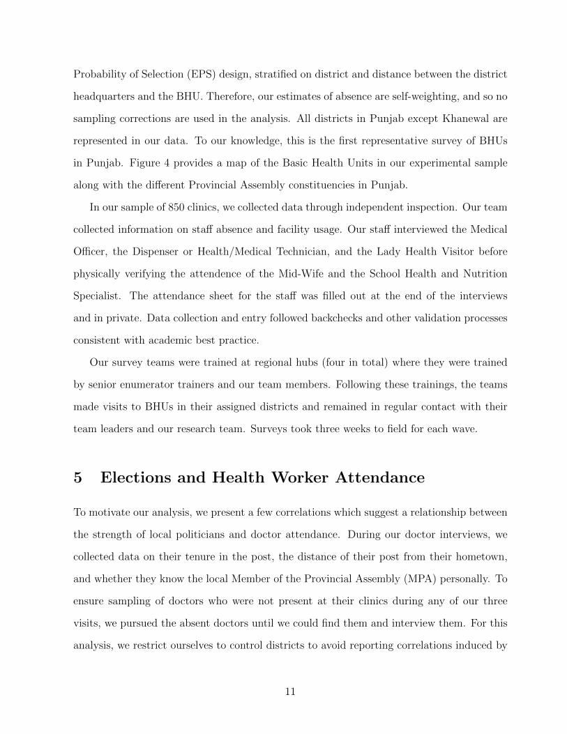
Probability of Selection (EPS) design, stratified on district and distance between the district

headquarters and the BHU. Therefore, our estimates of absence are self-weighting, and so no

sampling corrections are used in the analysis. All districts in Punjab except Khanewal are

represented in our data. To our knowledge, this is the first representative survey of BHUs

in Punjab. Figure 4 provides a map of the Basic Health Units in our experimental sample

along with the different Provincial Assembly constituencies in Punjab.

In our sample of 850 clinics, we collected data through independent inspection. Our team

collected information on staff absence and facility usage. Our staff interviewed the Medical

Officer, the Dispenser or Health/Medical Technician, and the Lady Health Visitor before

physically verifying the attendence of the Mid-Wife and the School Health and Nutrition

Specialist. The attendance sheet for the staff was filled out at the end of the interviews

and in private. Data collection and entry followed backchecks and other validation processes

consistent with academic best practice.

Our survey teams were trained at regional hubs (four in total) where they were trained

by senior enumerator trainers and our team members. Following these trainings, the teams

made visits to BHUs in their assigned districts and remained in regular contact with their

team leaders and our research team. Surveys took three weeks to field for each wave.

5 Elections and Health Worker Attendance

To motivate our analysis, we present a few correlations which suggest a relationship between

the strength of local politicians and doctor attendance. During our doctor interviews, we

collected data on their tenure in the post, the distance of their post from their hometown,

and whether they know the local Member of the Provincial Assembly (MPA) personally. To

ensure sampling of doctors who were not present at their clinics during any of our three

visits, we pursued the absent doctors until we could find them and interview them. For this

analysis, we restrict ourselves to control districts to avoid reporting correlations induced by

11

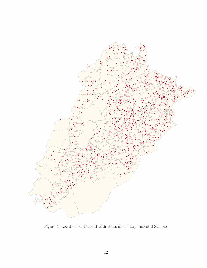
Figure 4: Locations of Basic Health Units in the Experimental Sample

12

our treatment.

Table 1 summarizes the data used for this analysis. The data reveal that doctor at-

tendance in our control districts is quite low. While our visits took place during normal

operating hours, we were able to locate doctors in only 22.5 percent of our visits. All BHUs

are supposed to have doctors posted. However, because of a combination of a shortage of

doctors, a lack of interest in rural postings, and perhaps misreporting to disguise absence,

we find that only 53.2 percent of BHUs have doctors posted. Even accounting for this low

rate of posting, doctor are present at only 42.29 percent of actual postings. Of the set of

doctors we observe, 24 percent report knowing the doctor personally.

Table 1: Summary Statistics

Variable Mean Standard Deviation # Observations

Doctor Present (=1) 0.225 0.418 1192Doctor Posted at Clinic (=1) 0.532 0.499 1192Doctor Knows Local MPA Personally (=1) 0.24 0.428 569Distance to Doctor’s Hometown (km) 122.765 302.062 204Doctor’s Months of Service 98.872 98.769 195Distance to District Headquarters (km) 49.065 28.781 1258Catchment Population (1,000) 24.777 8.547 1249Political Concentration 0.62 0.139 1259Victory Margin Share 0.157 0.106 1259

Notes: Sample: Control district clinics, survey waves 1 - 3. Political Concentration is a Herfindahl index

computed as the sum of squared vote shares for each party in a Provincial Assembly constituency ranging from

0.19 in the most competitive district to one in uncontested districts.

As we describe in Section 4, we identified the provincial assembly constituency in which

each of our clinics are located. In our control districts, we have BHUs in 124 constituencies.

We construct two measures of the degree of local electoral capture: “political concentration,”

a normalized Herfindahl index computed as the sum of squared vote shares for each party in

the constituency divided by the maximum Herfindahl score in our sample (0.55) and “Victory

Margin Share” which is simply the victory margin for the winning candidate as a share of

total votes cast in the local election. Political concentration ranges from 0.325 in the most

13

competitive constituency to one in uncontested constituencies.9 The victory margin share

in these 124 constituencies ranges from 0.0016 percent to 1 in uncontested districts. Figure

5 maps the political concentration measure for each constituency in Punjab. The degree of

political contestation appears only weakly correlated with geography.

In Table 2 we report correlations between these measures of local political competition

and doctor attendance. Columns (1) - (3) report regressions using the political concentra-

tion Herfindahl as an explanatory variable and (4) - (6) report the same specifications using

victory margin share. We find that doctors attend work more often in competitive con-

stituencies. In all specifications, we include Tehsil (county) fixed effects, which restricts our

variation to geographically proximate political constituencies that should be broadly similar

in terms of remoteness, climate, and desirability of doctor postings. While there are a range

of plausible omitted variables prohibiting a causal interpretation, we find that the correlation

is robust to including controls for catchment population, distance to the district center, and

whether a doctor was reported by other staff to be posted.

The results in Table 2 are consistent with two theories. First, it may be that in highly

competitive districts politicians face stronger incentives to make sure health services are

effectively delivered. Second, it may be that politicians who can capture districts are more

likely to provide sinecures as patronage. Doctors in patronage jobs may be expected to work

less. To investigate which of these is operative, we asked doctors whether they knew their

local MPA personally. 266 doctors were absent during all of our three visits. After our third

visit to the facilities, we pursued all 266 until we were able to interview them.

Table 3 examines whether doctors with a direct connection to the provincial assembly

member serving in their constituency are more likely to be absent. We run regressions of

the form:

Presenti = β0 + β1Knows Parliamentariani + εi (1)

9Before dividing by the maximum Herfindahl score in our sample, political concentration ranges from0.19 to 0.55

14

Normalized Herfindahl Index(0.42,1.00](0.37,0.42](0.34,0.37](0.28,0.34][0.00,0.28]

Figure 5: Electoral Competitiveness in Punjab (Normalized Herfindahl Index)

15

Table 2: Political Competition and Doctor Attendance

Dependent Variable: Doctor Present (=1)(1) (2) (3) (4) (5) (6)

Political Concentration -0.374*** -0.354** -0.176*(0.135) (0.136) (0.097)

Victory Margin -0.265 -0.297* -0.224*(0.178) (0.166) (0.120)

Distance to District Center (km) -0.002*** -0.001* -0.003*** -0.001**(0.001) (0.001) (0.001) (0.001)

Catchment Population (1,000) 0.004* 0.001 0.004** 0.001(0.002) (0.002) (0.002) (0.002)

Doctor Assigned (=1) 0.403*** 0.405***(0.031) (0.031)

Constant 0.465*** 0.488*** 0.140* 0.275*** 0.306*** 0.060(0.086) (0.111) (0.082) (0.029) (0.058) (0.048)

# Constituences 124 124 124 124 124 124# Observations 1190 1182 1182 1190 1182 1182R-Squared 0.158 0.170 0.322 0.154 0.167 0.322

Notes: *p < 0.1, **p < 0.05, ***p < 0.01. Sample: Control district clinics survey waves 1 - 3. Standard errors clustered

at the provincial assembly constituency level reported in parentheses. Sample: control district Basic Health Units (BHUs).

Political Concentration is a Herfindahl index computed as the sum of squared vote shares for each party in a constituency

ranging from 0.19 in the most competitive district to 1 in uncontested districts. All regressions include Tehsil (county)

and survey wave fixed effects.

for each doctor i in our sample. We record whether doctors are present on three separate

visits. Presenti therefore ranges between 0 and 3.

Columns (1) - (4) report results using only the 188 doctors posted in our control sample.

Column(5) reports the same specification for our entire sample. Doctors who do not know

their local MPA directly are present at an average of 1.237 of our 3 visits, while doctors who

do know their MPA are present at only 0.727 visits. These effects are robust to including

either district or Tehsil fixed effects, and including a range of controls. We provide further

support for the arguments that connected doctors enjoy preferential benefits in Table A1.

We find that doctors who know their local MPA are able to obtain postings closer to their

hometown, which are widely thought to be more desirable.

These correlations suggest that local politicians may secure office by providing sinecures

to supporters. This theory has predictions for the effectiveness of our experiment. Politically

connected inspectors and doctors should be less sensitive to monitoring. While monitoring

innovations increase the probability they are detected shirking, these incentives will not be

16

Table 3: Political Connections and Doctor Attendance

Dependent Variable: Number of Times Doctor Present (Max = 3)(1) (2) (3) (4) (5)

Doctor Knows Local MPA Personally (=1) -0.510*** -0.497*** -0.356** -0.462** -0.351***(0.133) (0.143) (0.158) (0.178) (0.123)

Patients Treated 0.000 -0.000 -0.000 0.000*(0.000) (0.000) (0.000) (0.000)

Catchment Population (1,000) -0.002 0.001 -0.005 -0.001(0.007) (0.007) (0.008) (0.004)

Distance to District Center (km) 0.004* 0.000 -0.003 -0.003(0.002) (0.003) (0.003) (0.002)

Doctor Assigned (=1) 0.757*** 0.630** 0.582* 0.954***(0.230) (0.262) (0.330) (0.207)

Constant 1.237*** 0.372 0.668** 1.013*** 0.469*(0.065) (0.279) (0.320) (0.377) (0.247)

# Observations 189 188 188 188 433R-Squared 0.057 0.112 0.223 0.383 0.435District Fixed Effects No No Yes No NoTehsil (County) Fixed Effects No No No Yes YesSample Controls Controls Controls Controls Full Sample

Notes: *p < 0.1, **p < 0.05, ***p < 0.01. Robust standard errors reported in parentheses. Sample: control district Basic

Health Units (BHUs). Political Concentration is a Herfindahl index computed as the sum of squared vote shares for each

party in a constituency ranging from 0.19 in the most competitive district to 1 in uncontested districts. All regressions

include Tehsil (county) and survey wave fixed effects.

binding for bureaucrats who are protected by their relations to local politicians.

6 Experimental Results

With this motivation as background, we now present our experimental results. Table 4

verifies balance in our experiment. As we discuss in Section 3, we stratified treatment on

the share of staff present during our baseline interview. While this achieved balance for five

of the six categories of staff that are supposed to be present at BHUs, we have a large and

significant imbalance for doctors. Figure A1 reports a long time series of administrative data

on doctor attendance. We find that the difference in levels does not reflect a difference in

pre-treatment trends, allaying concerns that our fixed effects estimates are not causal.10

We begin by examining the impact of treatment on health worker attendance. We test

10Note that this depicts the sample average. The effects we find on doctor attendance are localized to thesubsample of clinics in competitive districts.

17

Table 4: Randomization Verification

Conventional Smartphone Difference P-valueMonitoring (=1) Monitoring (=1)

BHU open during visit (=1) 0.926 0.930 -0.003 0.915[0.261] [0.256] (0.031)

Inspector Has Visited in the Last Month (=1) 0.234 0.214 0.020 0.731[0.424] [0.411] (0.057)

Number of Staff Present 2.729 2.874 -0.144 0.431[1.514] [1.638] (0.181)

Number of Staff Assigned 5.121 5.286 -0.165 0.199[0.924] [0.941] (0.126)

Medical Officer Present (=1) 0.234 0.412 -0.177 0.003[0.424] [0.493] (0.055)

Health Technician Present (=1) 0.398 0.347 0.050 0.379[0.490] [0.477] (0.057)

Dispenser Present (=1) 0.707 0.777 -0.070 0.277[0.456] [0.417] (0.063)

SHNS Present (=1) 0.348 0.340 0.008 0.890[0.477] [0.474] (0.059)

Lady Health Visitor Present (=1) 0.587 0.629 -0.042 0.422[0.493] [0.484] (0.052)

Midwife Present (=1) 0.538 0.474 0.064 0.164[0.499] [0.500] (0.045)

Political Concentration Herfindahl 0.620 0.615 0.005 0.8250.139 0.132 0.022

# of Observations 421 427

Notes: Level of significance: Variable standard deviations reported in brackets. Standard errors clustered at the district level

reported in parentheses.

for impacts on inspectors, where the program provides the sharpest incentives, doctors, and

total staff.

We estimate regressions of the form:

Ydit = α + βTreatmentdit +3∑

i=1

δt + λi + εit (2)

Ydit is health worker attendance or official inspection, where i refers to the clinic, d refers

to the district, and t to the survey wave. We cluster all standard errors at the district

level. With only 35 districts, we also use randomization inference. Figure 8 shows our actual

impact against impacts estimated from 1,000 hypothetical treatment assignments.

The first column verifies that the program increased inspections. The smartphone mon-

itoring system directly impacts health inspectors, as their activities are geostamped, times-

tamped, and observed in real time. We do not observe any significant average impacts on

18

0.10

0.30

0.50

0.70

Perc

ent f

acilit

ies

visite

d by

DDO

Nov. 2011 June 2012 Oct. 2012Month

Control Treatment

Figure 6: Effects by Survey Wave

doctor or overall staff attendance.

Panel B reports results splitting the treatment by survey wave 2 (May 2012) and wave 3

(October 2012). In column one, we see that the large impact on inspection has attenuated

somewhat over the life of the program. Inspections remain 89% higher than they were at

baseline. Figure 6 depicts attendance in treatment and control groups by wave. Future data

collection will indicate whether this downward trend sustains. In columns (2) - (5), we again

see no evidence of impact.

The correlations we find in Section 5 above suggest the possibility of heterogeneity by the

degree of political concentration. Popular accounts of local politics in Pakistan characterize

it broadly as a clientelistic system—a view strongly supported by our interviews with a select

group of experienced parliamentarians. Parliamentarians can influence both the allocation of

public sector jobs, and the enforcement of reporting requirements. We use the large degree of

19

Table 5: Impact on Inspections and Health Worker Attendance

Panel A - Average Effects Inspected (=1) Number of Staff Present Doctor Present (=1)(1) (2) (3) (4) (5)

Smartphone Monitoring (=1) 0.220*** -0.022 0.034 -0.016 -0.024(0.062) (0.230) (0.201) (0.044) (0.038)

# Staff Assigned 0.435***(0.039)

Doctor Assigned (=1) 0.368***(0.035)

Constant 0.217*** 2.803*** 0.538** 0.326*** 0.087***(0.022) (0.076) (0.213) (0.015) (0.028)

# Districts 35 35 35 35 35# Clinics 838 848 848 848 848# Observations 2167 2542 2542 2414 2414R-Squared 0.054 0.007 0.140 0.005 0.107

Panel B - Effects By Survey Wave Inspected (=1) Number of Staff Present Doctor Present (=1)(1) (2) (3) (4) (5)

Monitoring x Wave 2 0.300*** -0.144 -0.063 -0.035 -0.036(0.076) (0.251) (0.216) (0.056) (0.050)

Monitoring x Wave 3 0.146* 0.098 0.131 0.002 -0.013(0.079) (0.245) (0.216) (0.054) (0.048)

# Staff Assigned 0.434***(0.038)

Doctor Assigned (=1) 0.367***(0.035)

Constant 0.217*** 2.803*** 0.544** 0.326*** 0.087***(0.022) (0.076) (0.209) (0.015) (0.028)

# Districts 35 35 35 35 35# Clinics 838 848 848 848 848# Observations 2167 2542 2542 2414 2414R-Squared 0.063 0.009 0.141 0.006 0.107

Notes: *p < 0.1, **p < 0.05, ***p < 0.01. Standard errors clustered at the district level reported in parentheses. All regressions

include clinic and survey wave fixed effects.

20

variation in competitiveness across the 241 constituencies in our sample to check for impact

heterogeneity.

Table 6: Treatment Effects by Political Concentration

Dependent Var. Inspected (=1) Number of Staff Present Doctor Present (=1)(1) (2) (3) (4) (5)

Smartphone Monitoring (=1) 0.519** 1.390* 1.664** 0.321* 0.291*(0.225) (0.717) (0.736) (0.180) (0.163)

Monitoring x Political Concentration -0.485 -2.254* -2.626** -0.547** -0.514**(0.360) (1.265) (1.207) (0.264) (0.239)

# Staff Assigned 0.434***(0.035)

Doctor Assigned (=1) 0.368***(0.036)

Constant 0.217*** 2.804*** 0.545*** 0.327*** 0.087***(0.022) (0.074) (0.195) (0.014) (0.028)

# Districts 35 35 35 35 35# Clinics 836 845 845 845 845# Observations 2164 2534 2534 2410 2410R-Squared 0.056 0.014 0.144 0.009 0.110

Notes: *p < 0.1, **p < 0.05, ***p < 0.01. Standard errors clustered at the district level reported in parentheses. All regressions

include clinic and survey wave fixed effects.

Consistent with the correlations presented in Section 5, we find that monitoring leads to

a larger increase in attendance in competitive districts. The first column of Table 6 indicates

that our increase in monitoring is localized to competitive constituencies. Similarly, in

columns (2) and (3), we find that treatment results in roughly an additional worker being

present in the most competitive districts. Last, in columns (4) and (5) we find that doctors

are present at about 30 percent more facilities in competitive constituencies, with no effect

in noncompetitive constituencies.

21

−.2

0.2

.4.6

.8Tr

eatm

ent E

ffect

0 .2 .4 .6 .8 1Political Concentration

Dependent Variable: Inspected (=1)Treatment Effects by Political Concentration (with 95% CIs)

−2−1

01

23

Trea

tmen

t Effe

ct

0 .2 .4 .6 .8 1Political Concentration

Dependent Variable: Number of Staff PresentTreatment Effects by Political Concentration (with 95% CIs)

Figure 7: Treatment Effects by Political Concentration

22

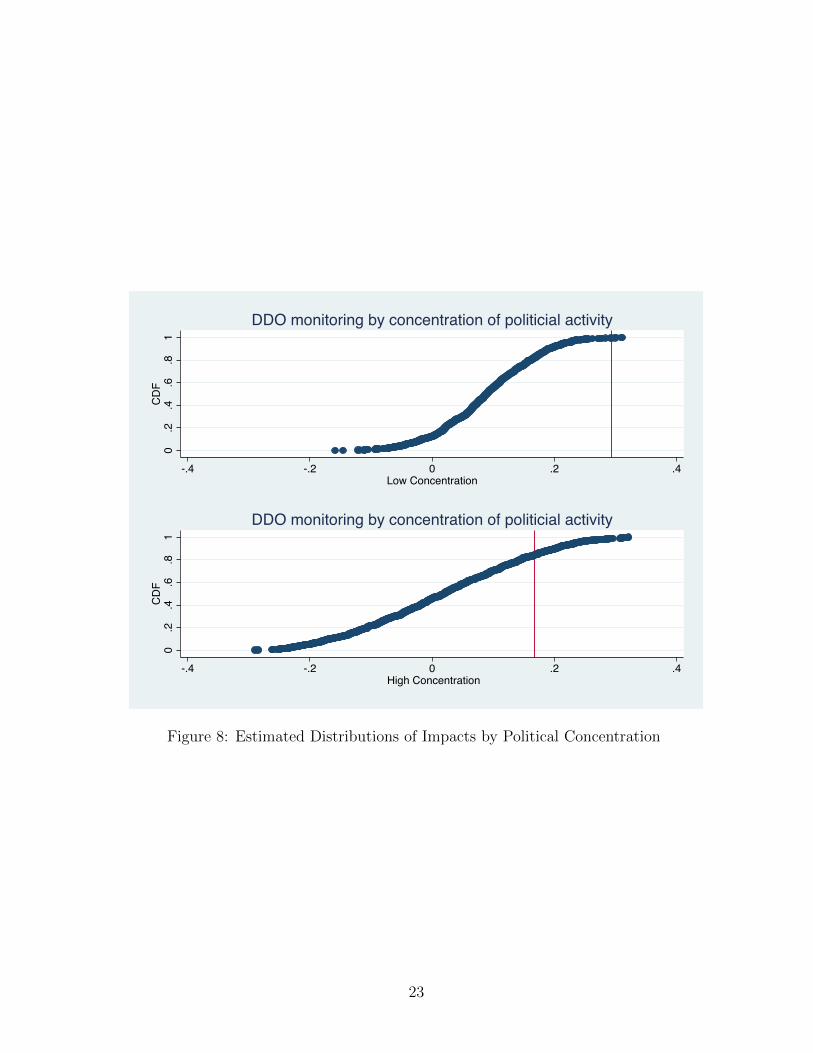
0.2

.4.6

.81

CDF

-.4 -.2 0 .2 .4Low Concentration

DDO monitoring by concentration of politicial activity

0.2

.4.6

.81

CDF

-.4 -.2 0 .2 .4 High Concentration

DDO monitoring by concentration of politicial activity

Figure 8: Estimated Distributions of Impacts by Political Concentration

23

7 Conclusion

In clientelistic systems, politicians gain office by providing targeted goods to supporters

instead of by effectively providing public goods. We examine a particular case: doctors

may be absent and unavailable to provide health care because their position is a sinecure

provided in return for political support. Three findings support this explanation for public

worker absence. First, absence is significantly more severe in less competitive districts.

Second, politically connected workers are absent more frequently. Third, the effects of a

novel monitoring regime on the performance of government monitors remain localized to

competitive districts.

Doctor, teacher, and other public worker absence is a serious obstacle to effective public

service delivery in developing countries (Banerjee and Duflo 2006; Chaudhury et al. 2006).

In many cases, it is also highly resistant to interventions aimed to promote attendance.

Understanding the political rationale for public worker absence opens a broader set of inter-

ventions to combat the problem. First, increasing voters awareness of public worker absence

might amplify the political costs from voters not motivated by patronage.11 Additionally,

professionalizing the civil service, and eliminating politicians involvement in decisions related

to bureaucratic hiring, firing, promotion, and posting would remove the opportunity to use

these positions as patronage.

More generally, anti-corruption efforts are rarely successful. Our findings suggest that

in some cases the resilience of public sector corruption may be because it is maintained

for reasons of political expedience. Given the huge potential payouts to politicians from

facilitating corruption, future research in the economics of corruption should consider the

political rationale for corruption. Such investigations could broaden the set of anti-corruption

policies and substantially increase their impact.

11Along these lines, Wilson (1961) states “organized guardians of the civic purse will not permit corruptpoliticoans to increase city expenditures through certain kinds of projects (for example, urban renewal, street-lighting, street-cleaning, building inspection, fire and police protection) but not through others (increasingthe staffs of aldermen, multiplying executive secretariats, and hiring men to do jobs which machines can dobetter—such as operating elevators, sweeping streets, etc.)”

24

References

Banerjee, Abhijit and Esther Duflo, “Addressing Absence,” The Journal of Economic

Perspectives, 2006, 20 (1), 117–132.

Banerjee, Abhijit V., Esther Duflo, and Rachel Glennerster, “Putting a Band-Aid

on a Corpse: Incentives for Nurses in the Indian Public Health Care System,” Journal of

the European Economic Association, 04-05 2008, 6 (2-3), 487–500.

Bates, Robert H., Markets And States In Tropical Africa: The Political Basis Of Agri-

cultural Policies California Series on Social Choice & Political Economy, University of

California Press, 1981.

Chaudhury, Nazmul, Jeffrey Hammer, Michael Kremer, Karthik Muralidharan,

and F. Halsey Rogers, “Missing in Action: Teacher and Health Worker Absence in

Developing Countries,” Journal of Economic Perspectives, Winter 2006, 20 (1).

Chubb, J., Patronage, Power and Poverty in Southern Italy: A Tale of Two Cities Cam-

bridge Studies in Modern Political Economies, Cambridge University Press, 1983.

Dahlberg, Matz and Eva Johansson, “On the Vote-Purchasing Behavior of Incumbent

Governments,” The American Political Science Review, March 2002, 96 (1), 27 – 40.

Dube, Arindrajit, Ethan Kaplan, and Suresh Naidu, “Coups, Corporations, and

Classified Information,” The Quarterly Journal of Economics, 2011.

Duflo, Esther, Rema Hanna, and Stephen P. Ryan, “Incentives Work: Getting Teach-

ers to Come to School,” The American Economic Review, 2012, 102 (4), 1241–1278.

Fisman, Raymond, “Estimating the Value of Political Connections,” American Economic

Review, 2001, 91 (4), 1095–1102.

Johnston, Michael, “Patrons and Clients, Jobs and Machines: A Case Study of the Uses

of Patronage,” The American Political Science Review, 1979, 73 (2), 385–398.

25

Khwaja, Asim Ijaz and Atif Mian, “Do Lenders Favor Politically Connected Firms?

Rent Provision in an Emerging Financial Market,” Quarterly Journal of Economics,

November 2005, 120 (4), 1371–1411.

Olken, Benjamin A. and Rohini Pande, “Corruption in Developing Countries,” Annual

Review of Economics, 2012, 4, 479–505.

Robinson, James A and Thierry Verdier, “The Political Economy of Clientelism,”

CEPR Discussion Paper 3205, C.E.P.R. Discussion Papers February 2002.

Sorauf, Frank J., “State Patronage in a Rural County,” American Political Science Review,

December 1956, 50 (4), 1046–1056.

Wilson, James Q., “The Economy of Patronage,” Journal of Political Economy, August

1961, 69 (4), 369–380.

26

020

4060

8010

0Pe

rcen

t of C

linic

s w

ith D

r. Pr

esen

t

Augus

t 201

1

Novem

ber 2

011

Februa

ry 20

12

May 20

12

Control Treatment

Figure A1: Average Doctor Attendance Before and After Treatment

27

Tab

leA

1:C

onnec

tion

san

dP

erks

Dep

enden

tV

aria

ble

:D

ista

nce

toD

oct

or’s

Hom

etow

n(k

m)

(1)

(2)

(3)

(4)

(5)

(6)

(7)

Doct

orK

now

sM

PP

erso

nal

ly(=

1)-1

31.6

28**

*-1

12.9

18**

*-1

27.6

07**

*-9

5.36

6**

-270

.811

***

-314

.565

-393

.636

*(3

5.43

1)(3

5.67

5)(4

1.79

2)(4

6.48

5)(8

3.03

0)(1

88.2

70)

(212

.932

)D

oct

or’s

Yea

rsof

Ser

vic

e0.

093

0.03

51.

977

(0.3

07)

(0.3

61)

(1.5

78)

Cat

chm

ent

Pop

ula

tion

(1,0

00)

-1.9

50-1

.417

-5.5

50(2

.579

)(2

.471

)(1

1.66

8)D

ista

nce

toD

istr

ict

Cen

ter

(km

)1.

066

2.02

30.

995

(0.8

99)

(1.2

40)

(4.3

10)

Con

stan

t19

8.69

8***

185.

783*

**19

1.74

8**

126.

098

449.

808*

**46

0.51

2***

444.

783

(47.

187)

(42.

578)

(95.

577)

(90.

661)

(105

.185

)(9

9.94

8)(3

64.0

98)

Dis

tric

tF

ixed

Eff

ects

No

Yes

Yes

No

No

Yes

Yes

Teh

sil

(Cou

nty

)F

ixed

Eff

ects

No

No

No

Yes

No

No

No

Sam

ple

Full

Full

Full

Full

>50

km

>50

km

>50

km

#O

bse

rvat

ions

204

204

194

194

6060

56R

-Squar

ed0.

045

0.21

40.

233

0.38

50.

063

0.42

90.

494

Note

s:*p<

0.1,

**p<

0.05

,***p<

0.01.

Sta

nd

ard

erro

rscl

ust

ered

atth

eB

asic

Hea

lth

Un

it(B

HU

)le

vel

rep

orte

din

pare

nth

eses

.S

am

ple

:F

ull

-co

ntr

ol

dis

tric

tB

HU

s;>

50k

m-

contr

olB

HU

sw

her

ed

oct

oris

furt

her

than

50km

from

thei

rh

omet

own

.A

llre

gre

ssio

ns

incl

ud

eT

ehsi

l(c

ou

nty

)an

dsu

rvey

wav

e

fixed

effec

ts.

28