Factors Affecting the Exchange Rate Risk Premium 6_6_3.pdf · other factors have a significant...
23
Journal of Applied Finance & Banking, vol. 6, no. 6, 2016, 33-55 ISSN: 1792-6580 (print version), 1792-6599 (online) Scienpress Ltd, 2016 Factors Affecting the Exchange Rate Risk Premium Dr. Ioannis N. Kallianiotis 1 Abstract The objective of this work is to identify and examine the risk premium of the exchange rate; then, to determine the factors that cause it, and to measure its variance by using a GARCH-M model. Some theoretical models are developed by taking the exchange rate risk premium as dependent variable and other macro- variables, political events, and market conditions as independent ones. There are three different exchange rates ($/€, $/£, and ¥/$) used, here, for the measurement of the risk premium and the empirical test of the model. The empirical results show that the variances of our macro-variables, the policy variables (interest rates and money supply), the price of oil, the war in Iraq, the European debt crisis, and other factors have a significant effect on the risk premium. Also, the conditional variances of the stock markets risk premium are having a highly significant effect on the exchange rate risk premia. The empirical results show that the foreign exchange market is not very efficient and the monetary policy not very effective. JEL classification numbers: C13, C22, C53, F31, F41, F42, G14 Keywords: Estimation, Time-Series Models, Forecasting and Other Model Applications, Foreign Exchange Risk: Time-Varying Risk Premium, Open Economy Macroeconomics, International Policy Coordination, Information and Market Efficiency: Event Studies 1 Introduction The exchange rates do not have a constant mean and exhibit phases of relative tranquility followed by periods of high volatility (no constant variance). 2 We want 1 Economics/Finance Department, The Arthur J. Kania School of Management, University of Scranton, Scranton, PA 18510-4602, U.S.A. 2 If the variance of a stochastic variable is not constant [ 2 2 ) ( t E ], it is called heteroskedastic. Article Info: Received : July 11, 2016. Revised : August 2, 2016. Published online : November 1, 2016
Transcript of Factors Affecting the Exchange Rate Risk Premium 6_6_3.pdf · other factors have a significant...
Journal of Applied Finance & Banking, vol. 6, no. 6, 2016, 33-55
ISSN: 1792-6580 (print version), 1792-6599 (online)
Scienpress Ltd, 2016
Factors Affecting the Exchange Rate Risk Premium
Dr. Ioannis N. Kallianiotis1
Abstract
The objective of this work is to identify and examine the risk premium of the
exchange rate; then, to determine the factors that cause it, and to measure its
variance by using a GARCH-M model. Some theoretical models are developed by
taking the exchange rate risk premium as dependent variable and other macro-
variables, political events, and market conditions as independent ones. There are
three different exchange rates ($/€, $/£, and ¥/$) used, here, for the measurement
of the risk premium and the empirical test of the model. The empirical results
show that the variances of our macro-variables, the policy variables (interest rates
and money supply), the price of oil, the war in Iraq, the European debt crisis, and
other factors have a significant effect on the risk premium. Also, the conditional
variances of the stock markets risk premium are having a highly significant effect
on the exchange rate risk premia. The empirical results show that the foreign
exchange market is not very efficient and the monetary policy not very effective.
JEL classification numbers: C13, C22, C53, F31, F41, F42, G14
Keywords: Estimation, Time-Series Models, Forecasting and Other Model
Applications, Foreign Exchange Risk: Time-Varying Risk Premium, Open
Economy Macroeconomics, International Policy Coordination, Information and
Market Efficiency: Event Studies
1 Introduction
The exchange rates do not have a constant mean and exhibit phases of relative
tranquility followed by periods of high volatility (no constant variance).2 We want
1 Economics/Finance Department, The Arthur J. Kania School of Management, University of
Scranton, Scranton, PA 18510-4602, U.S.A. 2 If the variance of a stochastic variable is not constant [
22 )( tE ], it is called heteroskedastic.
Article Info: Received : July 11, 2016. Revised : August 2, 2016.
Published online : November 1, 2016

34 Ioannis N. Kallianiotis
to see and examine the behavior of these time series, here, and to model the
conditional heteroskedasticity (ARCH or GARCH).3 By graphing the following
three exchange rates: €/$, £/$, and ¥/$,4 we see that these series are not stationary;
their means do not appear to be constant and there is a strong heteroskedasticity.
They have time-varying means (they are not stationary). These exchange rates
show that they go through sustained periods of appreciation and then depreciation
with no tendency to revert to a long-run mean. This type of random walk behavior
is typical of nonstationary series.5 Enormous shocks were the central banks’ target
rates persistence with a violently very low value (closed to zero) for seven or more
years. Also, the volatility of many macro-variables was not constant over time.
Globalization has made the macro-variables in the four countries and economies
(U.S., Euro-zone, U.K., and Japan) to share co-movements. We want to identify
and estimate the risk premia of these three exchange rates.
The objective is to model and forecast the volatility (conditional variance)
of our variables. We need to analyze the risk of holding a specific currency. This
can be done by determining these variables that affect the exchange rate risk
premium and forecasting the variance of their errors. Then, more efficient
estimates can be obtained if heteroskedasticity in the errors is handled properly.
Autoregressive Conditional Heteroskedasticity (ARCH) models are specifically
designed to model and forecast conditional variances. The variance of the
dependent variable is modeled as a function of past values of the dependent
variable [AR (p) process] and independent or exogenous variables.
In other words, we want to forecast the risk premia and their variances
over time. The approach can be to explicitly introduce independent variables,
based on some economic theory and to predict their volatility. Financial
economists try to establish a relationship between exchange rate risk premia and
the measure of risk. One popular approach is the consumption-based international
3 ARCH = Autoregressive Conditional Heteroskedastic model and GARCH = Gerneralized
Autoregressive Conditional Heteroskedasticity. In Statistics, a collection of random variables is
heteroscedastic [or “heteroskedastic”; from Ancient Greek ἕτερον (hetero = “different”) and
σκέδασις (skedasis = “dispersion”)] if there are sub-populations that have different variabilities
from others. Here “variability” could be quantified by the variance or any other measure of
statistical dispersion. Because heteroskedasticity concerns expectations of the second moment of
the errors, its presence is referred to as misspecification of the second order. 4 Graphs, Figures, and many Tables are omitted, here, due to space constraints, but they are
available from the author upon request. 5 The test of stationary (Augmented Dickey-Fuller Unit Root Test) shows: (1) Indirect quotes for
the U.S. dollar: S1(€/$): -1.417 I(1); D(S1): -11.349***
I(1). S2(£/$): -2.833*I(0); D(S2): -
16.323***
I(1). S3(¥/$): -2.647*
I(0); D(S3): -16.440***
I(1). (2) Direct quotes for the U.S. dollar: S1΄
($/€): -1.514 I(1); D(S1΄): -11.858***
I(1). S2΄($/£): -2.736*I(0); D(S2΄): -15.794
***I(1). S3΄($/¥): -
1.750 I(1); D(S3΄): -16.696***
I(1). [I(0) = series contain zero unit roots (stationary), I(1) = series
contains one unit root (integrated order one, nonstationary), D(S) = variable in 1st differences,
*significant at the 10% level,
**significant at the 5% level, and
***significant at the 1% level].

Factors Affecting the Exchange Rate Risk Premium 35
Asset Pricing Model,6 which built on the promise that the economic agent chooses
an optimal time path of consumption and assets that yield uncertain returns. Some
empirical results have shown that movements in the conditional risk premia of
returns on the U.S. stock market are similar to those of the conditional risk premia
in the forward foreign exchange markets. Attempts have been made to establish an
empirical link between the exchange risk premium and these financial variables.
The historical data show that: (1) 218.11 S $/€, 032231.02
1S , the
expected 002449.011
e
tt
e
t rpfs and 0010763.02
1
etrp
, the actual
006704.03 ttt RPFS , 00445089.02
1RP , and ln of the actual
005453.03 ttt rpfs , 00245213.02
1rp . (2) 760.12 S $/£,
094608.02
2S , 000104.01
e
trp , 000915728.02
1
etrp
, 003693.0tRP ,
0055662.02
1RP , and 002163.0trp , 001939698.02
1rp . (3) 874.1633 S
¥/$, 6814.535,52
3S , 001770.01
e
trp , 001189836.02
1
etrp
, 226191.0tRP
, 1817.322
1RP , and 001455.0trp , 00256948.02
1rp .
2 Some Theories of Exchange Rate Risk Premium Determination
Some researchers have related the expected and realized return in the foreign
exchange markets to the nominal interest rates (monetary policy target rates and
IRP condition) as follows,7
1*
210*
1 )( ttttttt iiiiss (1)
where, 01 , 02 , tttt fiis )( * is the covered interest parity condition, and if
01 tt fs this is the exchange rate risk premium ( 1trp ), which shows foreign
exchange market inefficiency.
The forecasting of the expected spot exchange rate ( e
ts 1) can be done by
using an ARMA (p, q) process or the following equation:
tttttttttt iiiiffsss
*
28
*
172615241322110 (1΄)
6 See, Mehra [16].
7 See, Kallianiotis [15, 107-114]. Also, see, Giovannini and Jorion [13].

36 Ioannis N. Kallianiotis
Now, we know the coefficients ( s
) and updating one period the variables of the
above eq. (1΄), we receive the 1tt sE conditional on the information available at
period t.
Also, by decomposing the nominal interest rate ( ti ) into two components,
real ( tr ) and expected inflation ( et ), eq. (1) can be written,
1**
210*
1 )()()( te
ttetttttt rriiss (2)
where, 01 , 02 .
Thus, increases in foreign exchange risk premia, that is, higher values of (
11 ttt rpfs ) are reliably associated with decreases in U.S. interest rates and
increases in foreign interest rates.8 Also, this holds for a decrease in the U.S. real
rate of interest and the expected inflation or an increase in the foreign real rate and
foreign expected inflation. We assume: *
tt rr and we forecast the e
t and the e
t
* .
Also, assuming that et
et m and e
te
t m** , monetary policy can affect the foreign
exchange market.
In addition, we take the money demand equation and making the money
demand equal to the money supply at their equilibrium point, we have the
following general function in natural logarithm term:
),,( tttt ipyfm (3)
where, tm = ln of money supply, ty = ln of income, tp = ln of the price level (CPI),
and ti = the short term interest rate.
Solving eq. (3) for ti , we receive:
),,( tttt pymfi (4)
And for the foreign country, we will have a similar relationship:
),,( ****
tttt pymfi (5)
where, an asterisk (*) denotes the foreign variables.
8 This holds for the UKS and the UKF:
UKt si )(* and
UKt fi )(*.
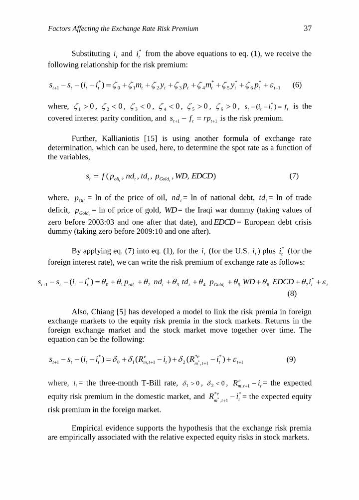
Factors Affecting the Exchange Rate Risk Premium 37
Substituting ti and *
ti from the above equations to eq. (1), we receive the
following relationship for the risk premium:
1
*
6
*
5
*
43210
*
1 )( ttttttttttt pympymiiss (6)
where, 01 , 02 , 03 , 04 , 05 , 06 , tttt fiis )( * is the
covered interest parity condition, and 11 ttt rpfs is the risk premium.
Further, Kallianiotis [15] is using another formula of exchange rate
determination, which can be used, here, to determine the spot rate as a function of
the variables,
),,,,,( EDCDWDptdndpfstt Goldttoilt (7)
where, tOilp = ln of the price of oil, tnd = ln of national debt, ttd = ln of trade
deficit, tGoldp = ln of price of gold, WD= the Iraqi war dummy (taking values of
zero before 2003:03 and one after that date), and EDCD = European debt crisis
dummy (taking zero before 2009:10 and one after).
By applying eq. (7) into eq. (1), for the ti (for the U.S. ti ) plus *
ti (for the
foreign interest rate), we can write the risk premium of exchange rate as follows:
ttGoldttoiltttt iEDCDWDptdndpiisstt
*
76543210
*
1 )(
(8)
Also, Chiang [5] has developed a model to link the risk premia in foreign
exchange markets to the equity risk premia in the stock markets. Returns in the
foreign exchange market and the stock market move together over time. The
equation can be the following:
1
**
1,21,10
*
1 )()()( * tt
e
tmt
e
tmtttt iRiRiiss (9)
where, ti = the three-month T-Bill rate, 01 , 02 , t
e
tm iR 1, = the expected
equity risk premium in the domestic market, and **
1,* t
e
tmiR
= the expected equity
risk premium in the foreign market.
Empirical evidence supports the hypothesis that the exchange risk premia
are empirically associated with the relative expected equity risks in stock markets.

38 Ioannis N. Kallianiotis
3 Multivariate GARCH-in-Mean Model
In conventional econometric models, the variance of the disturbance term is
assumed to be constant. Thus, a stochastic variable with a constant variance
[ 22 )( tE ] is called homoskedastic; but, if the variance is not constant
[ 22 )( tE ], it is called heteroskedastic. The exchange rate series show no
particular tendency to increase or decrease. The U.S. dollar seems to go through
sustained periods of appreciation and then depreciation, especially with respect the
yen and the euro, with no tendency to revert to a long-run mean. This type of
random walk behavior is typical of nonstationary series, I(1) for $/€ and $/¥ (they
seem to meander). When the volatility of a series is not constant over time, we call
it conditionally heteroskedastic.
We can model the distribution of the excess return (or money) in the foreign
exchange market jointly with the other macroeconomic factors. Since the
conditional mean of the excess return depends on time-varying second moments
of the join distribution, we require an econometric specification that allows for a
time-varying variance-covariance matrix. A choice can be the multivariate
GARCH-in-Mean (GARCH-M) model.9
We begin with the simplest GARCH (1, 1) specification:
ttt Xrp ' (10) 2
1
2
1
2
ttt (11)
Where, the mean equation (10) is written as a function of exogenous macro-
variables ( tX΄ ) from both countries [i. e., eqs. (1) or (2) or (6) or (8) or (9)] with
an error term t . Since 2
t is the one-period ahead forecast variance based on
current information, it is the conditional variance. This conditional variance
specified in eq. (11) is a function of three terms: The constant term ; news about
volatility from the previous period, measured as the squared residual from the
mean equation 2
t (the ARCH term); and the current period’s forecast variance 2
t
(the GARCH term).
This specification can be interpreted as follows. A trader in foreign
currency predicts this period’s variance by forming a weighted average of a long
term average (the constant ), the forecasted variance from the current period
(the GARCH term 2
t ), and information about the volatility observed in the
current period (the ARCH term 2
t ). If the exchange rate volatility ( trp ) was
9 See, Engle, Lilien, and Robins [11]. Also, Smith, Soresen, and Wickens [18].
Factors Affecting the Exchange Rate Risk Premium 39
unexpectedly large in either the upward or the downward direction; then, the
trader will increase the estimate of the variance for the next period.10
A higher order GARCH model, GARCH (q, p), can be estimated by
choosing either q or p greater than 1, where q is the order of the autoregressive
GARCH terms and p is the order of the moving average ARCH terms. The
GARCH (q, p) variance is:
p
iiti
q
jjtjt
1
2
1
22 (12)
The tX΄ in eq. (10) represent exogenous or pre-determined macro-
variables from both countries included in the mean equation. By introducing the
conditional variance into the mean equation, we get the GARCH-in Mean
(GARCH-M),11
as follows:
tttt Xrp 2' (13)
Equation (12) can be extended to allow for the inclusion of exogenous or
pre-determined regressors, tZ΄ , in the variance equation, as follows:
'
1
2
1
22
t
p
iiti
q
jjtjt Z
(14)
The forecasted variance can be positive or negative. The best for us can be
to introduce regressors in a form where they are always positive to minimize the
possibility that a single large negative value generates a negative forecasted value.
4 Data and Estimation of the Model
The data are monthly and are coming from Economagic.com, Eurostat, and
Bloomberg. For the euro (€) the data are from 1999:01 to 2015:12 and for the
other two currencies pound (£) and yen (¥) from 1971:01 to 2015:12. Other data
are the 3-month T-bill rates, the money supply (M2), the real income, the
consumer price index, the price of oil, the national debt, the current account, the
price of gold, the stock market indexes, and two dummies: (1) WD = the war
10
This model specification is also consistent with the volatility clustering often seen in financial
return data, where large changes in returns are likely to be followed by further large changes. 11
The GARCH-M model is often used in financial applications where the expected return on an
asset is related to the expected asset risk. The estimated coefficient on the expected risk is a
measure of the risk-return tradeoff.
40 Ioannis N. Kallianiotis
dummy in Iraq (with 0 before 2003:03 and 1 after 2003:04) and (2) EDCD = the
European debt crisis dummy (with 0 before 2009:09 and 1 after 2009:10).
The estimation accompanies the four (4) following steps:
1st : We forecast the e
ts 1 in eq. (1) as follows:
tttttttttt iiiiffsss
*
28
*
172615241322110
(1΄΄)
and we receive the SFse
t 1 (spot forecasting) from the computer forecasting it
for next period (by forwarding for one period). We can use an ARMA (p, q)
process or eq. (7), too.
2nd
: We run eqs. (1), (2), (6), (8), and (9) and determine the error terms ( t ) of
these five different risk premium specifications.
3rd
: We determine (estimate) the GARCH (p, q) equation of the above five risk
premia models [eq. (11)].
4th
: We incorporate the GARCH results into eqs. (1), (2), (6), (8), and (9) to see
the effects of the variance of the different variables on the exchange rate risk
premium ( trp ) or we can run the mean equation (upper part) and the lower part the
variance equation, eq. (13), simultaneously.
The empirical results show that the sum of the ARCH and GARCH
coefficients ( ) is very close to one (1), indicating that volatility shocks are
quite persistent. These results are often observed in high frequency financial data.
We start forecasting the e
ts 1 by using eq. (1΄), which gives some very good
statistics and very small RMSEs. Table 1 presents the GARCH estimation of eq.
(1), the e
trp 1 by using eq. (13), the conditional variance of the risk premium ( rp ).
We see that the residual (ARCH) is not highly significant, but the variance
(GARCH) is highly significant at 1% level.
Then, we forecast the ln of price level ( e
tp ), the expected inflation ( e
t ),
and the ln of money supply ( e
tm ). Tables 2, 3, and 4 show the estimation of eq.
(13) for the above three groups of variables ( e
tp , e
t , and e
tm ) by using the
GARCH-M model. The GARCH-M model shows significant effects of ARCH
and GARCH on the variance of the e
trp 1.
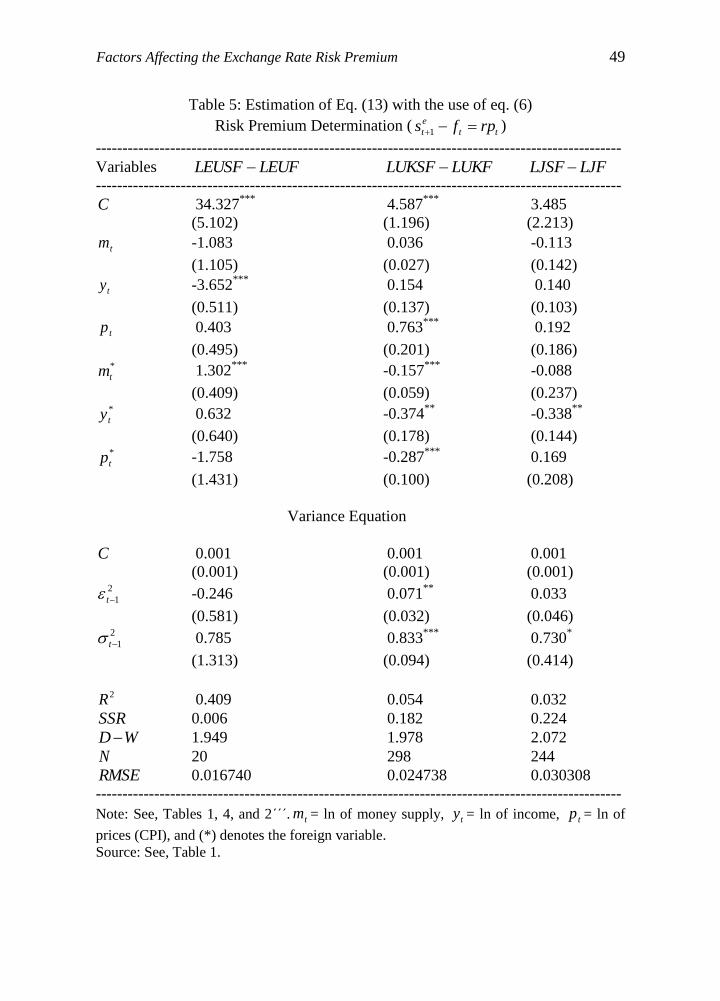
Further, the estimation of eq. (6) takes place and Table 5 gives the
estimation of eq. (13) by using eq. (6) to determine the rp as a function of
GARCH-M, which is significant only for the dollar/pound exchange rate e
trp 1.
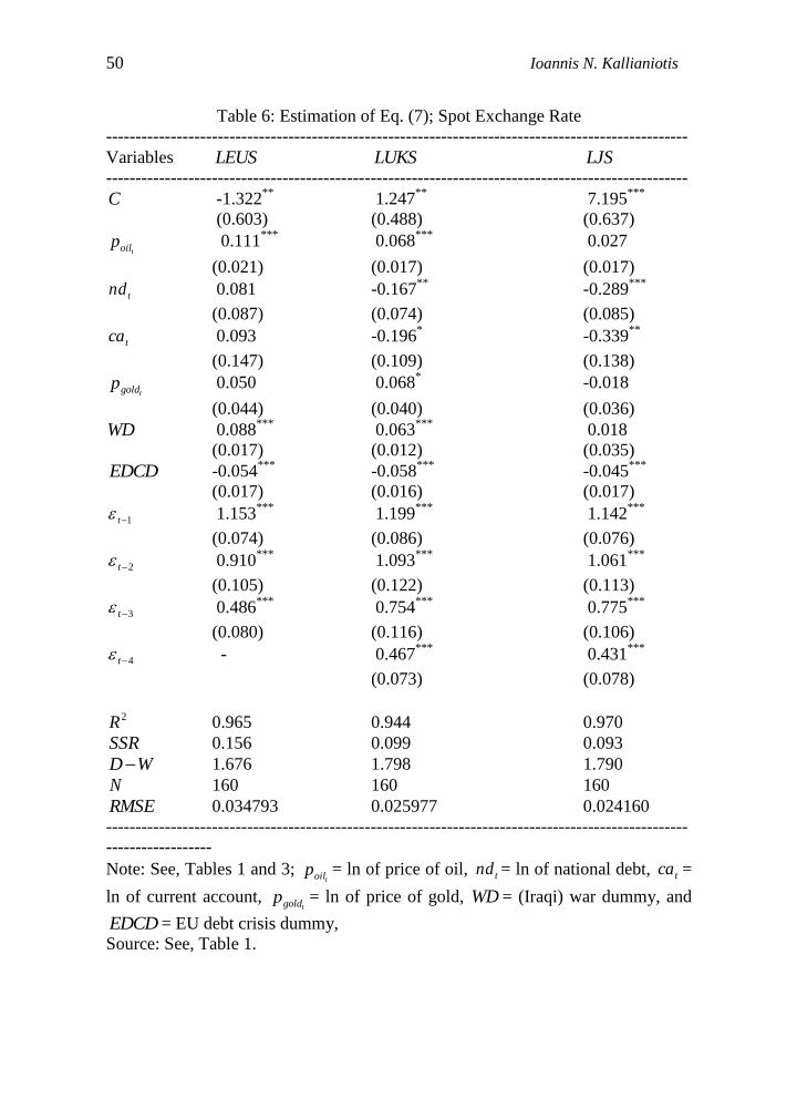
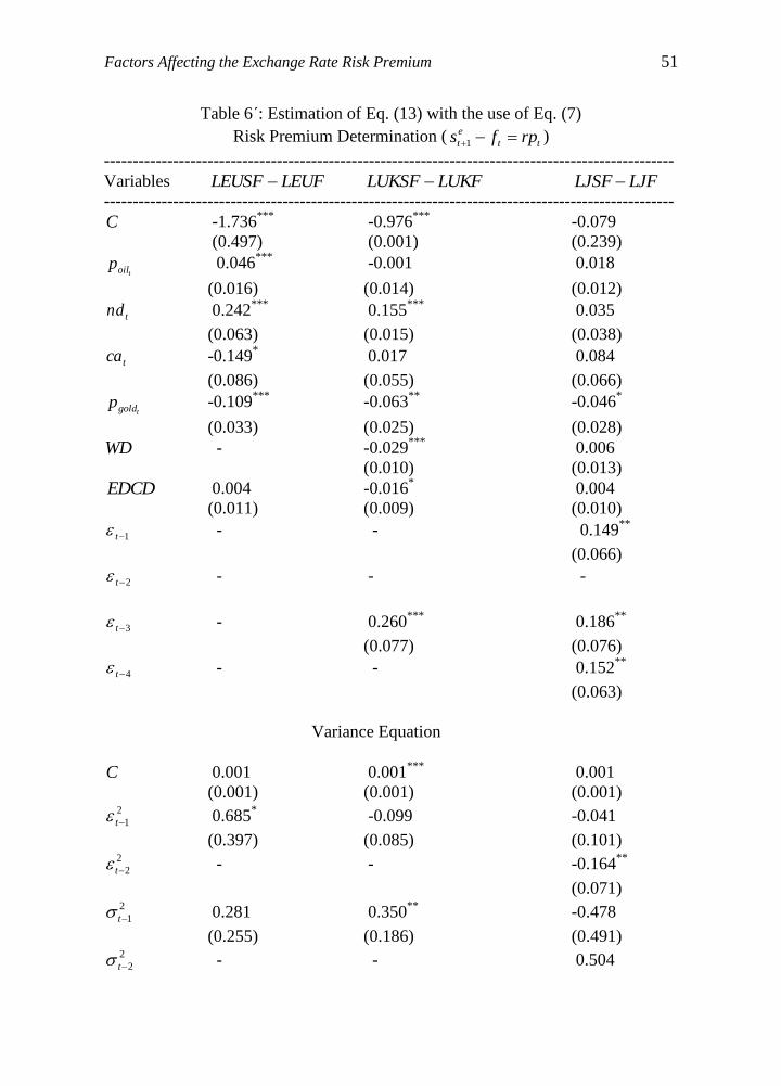
Table 6 estimates eq. (7) and Table 6΄ estimates the risk premium of the same eq.
(7) with the use of GARCH-M. The war dummy (WD) and the European debt
crisis dummy (EDCD) have the correct expected signs (+ and -) and have
significant effects on spot rate ($/€) and on the trp ; but the GARCH-M

Factors Affecting the Exchange Rate Risk Premium 41
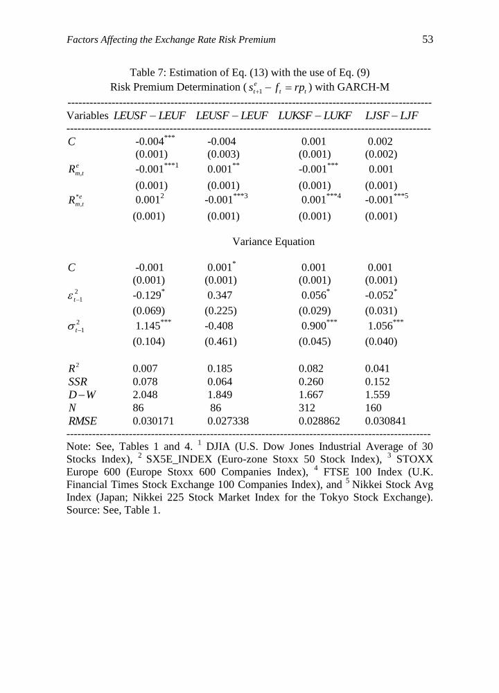
specification is not very effective. Lastly, Table 7 gives the estimation of eq. (13)
by using eq. (9), the stock market risk premium. It shows significant effects (at 1%
level) of the market risk premium and CARCH-M on the exchange rate risk
premia, except the Euro Stoxx 600 Companies Index.
Here, the forecasted variances are all positive, except the $/£ in eq. (1), $/€
in eq. (9) and $/£ in eq. (9), which is good for us because we will have a positive
forecasted value.
Figures 1΄and 1΄΄ show the static and dynamic forecasting of the e
trp 1
($/€), where the variance is not constant and it is growing overtime. Also, the
static and dynamic forecasting of the e
trp 1 ($/£), show that the variance is not
constant, but it is declining overtime. Further, the static and dynamic forecasting
of the e
trp 1 (¥/$) give that the variance is not constant and it is increasing with the
passing of time.
Furthermore, the static and dynamic e
trp 1 ($/€) with respect the stock
market risk premium (DJIA and Euro Stoxx 50 Index) display that the variance is
not constant and is growing over time. The static and dynamic e
trp 1 ($/€) with the
stock market risk premium (DJIA and Stoxx Europe 600 Index) present that the
variance is falling at the beginning and stays constant after 2005.
Finally, the static and dynamic e
trp 1 ($/£) with respect the stock market
risk premia (DJIA and FTSE 100 Index) reveal that the variance is not constant
and it is declining over time. The static and dynamic forecasting of the e
trp 1 (¥/$)
with their effects from the stock market risk premia (DJIA and Nikkei Stock Avg
Index) show that the variance is not constant and is increasing overtime.
5 Conclusion
The aim of this research was to determine the factors that affect the exchange rate
risk premium. From the historical data for three different exchange rates ($/€, $/£,
and ¥/$), we see that there are historic risk premia, which are mentioned in section
I above. By graphing these three exchange rates, we observe that they do not have
a constant mean and exhibit phases of relative tranquility and also of high
volatility, which means that they have no constant variance. For this reason, we
model the conditional heteroskedasticity (GARCH) of their risk premia. Some
series share co-movements with other series even in other countries. The
underlying economic forces that affect the U.S. economy affect also the
economies of other countries, due to globalization (high correlation between U.S.
and foreign economies; i.e., 1.,. EUSU ). The analysis show that pure monetary
policies are not effective and cannot improve efficiency, growth, stability,
confidence, and certainty in our complex interdependent economies.
42 Ioannis N. Kallianiotis
The theoretical models are using as independent variables, policy variables
( ti and s
tM ), inflation, income (production), price of oil, national debt, trade
deficit, stock market premium, and other events (war in Iraq and European debt
crisis) to determine their effects on the exchange rate risk premium ( trp ). The
multivariate GARCH-in-Mean models determine the volatility of the exchange
rate and then, the foreign currency trader can increase the estimate of the variance
for next period, if the volatility is unexpectedly large.
Lastly, the empirical results show a very good forecasting of the exchange
rates based on our model and reveal also a significant effect of the squared
residuals (ARCH) and the variance (GARCH term) on the exchange rate risk
premia. The war in Iraq12
has depreciated the U.S. dollar ($) and the European
debt crisis has depreciated the euro (€) and appreciated the dollar ($). Lately, the
possibility of the exit of U.K. from the EU hs affected negatively the value of the
British pound and the stock markets, too.13
The static and dynamic forecasting of
the e
trp 1 show that their variances are not constant and are increasing overtime,
except the ($/£) exchange rate, which is falling. The stock market volatility has a
high significant effect on the risk premia for the three exchange rates, which can
be seen also graphically with the forecasting of its variance. The variances are not
constant, too and mostly are increasing overtime, except for the ($/£) exchange
rate and the stock market risk premia (DJIA and FTSE 100 Index). Foreign
exchange markets are not very efficient. The next step of this research must be the
use of some different diagnostic and model specification tests to improve our
confidence regarding the theoretical models.
AKNOWLEDGEMENTS. I would like to acknowledge the assistance provided by
Jerry Zolotukha, Angela J. Parry, and Janice Mecadon. Financial support
(professional travel expenses, submission fees, etc.) was provided by Provost’s
Office (Faculty Travel Funds, Henry George Fund, and Faculty Development
Funds). The usual disclaimer applies. Then, all remaining errors are mine.
12
This was the beginning of the Middle East crisis (March 2003), which was spread from Iraq to
Afghanistan to Syria and all over the area and in North Africa (Libya) and now, to Europe (mostly
in Greece) with these millions of illegal immigrants. This suspicious crisis that was generated by
the West has increased the global risk (systemic) and has a significant economic and social effect
on the western economies. 13
Labour Party lawmaker, Jo Cox, was murdered on June 15, 2016, who was in favor of “YES” in
the EU referendum. See, http://www.express.co.uk/finance/city/658338/Brexit-EU-Exit-How-
Affect-Pound-UK-Economy. Also,
http://www.bloomberg.com/news/articles/2016-06-17/u-k-parliament-to-pay-tribute-to-murdered-
cox-before-eu-vote
Factors Affecting the Exchange Rate Risk Premium 43
References
[1] Bollerslev, Tim, Generalized Autoregressive Conditional Heteroskedasticity,
Journal of Econometrics, 31, (1986), 307-327. [2] Carlson, John A. and Carol L. Osler, Currency Risk Premiums: Theory and
Evidence, (2003), 1-51.
[3] Carlson, John A. and C.L. Osler, Determinants of Currency Risk Premiums,
Federal Reserve Bank of New York, (1999), 1-42.
[4] Cheung, Yin-Wong, Exchange Rate Risk Premiums, Journal of International
Money and Finance, 12, (1993), 182-194.
[5] Chiang, T., International Asset Pricing and Equity Market Risks, Journal of
International Money and Finance, Vol. 10, September, (1991), 365-391.
[6] Della Corte, Pasquale, Tarun Ramadorai, and Lucio Sarno, Volatility Risk
Premia and Exchange Rate Predictability, National Bank of Serbia, March
(2013) 1-49.
[7] Enders, Walter, Applied Econometric Time Series, John Wiley & Sons, Inc.,
New York, 1995.
[8] Engel, Charles, Exchange Rates, Interest Rates, and the Risk Premium,
NBER Working Paper 21042, (2015), 1-66.
[9] Engel, Charles, On the Foreign Exchange Risk Premium in a General
Equilibrium Model, Journal of International Economics, 32, (1992), 305-319.
[10] Engle, Robert F., Autoregressive Conditional Heteroskedasticity with
Estimates of the Variance of U.K. Inflation, Econometrica, 50, (1982), 987-
1008.
[11] Engle, Robert F., David M. Lilien, and Russell P. Robins, Estimating Time
Varying Risk Premia in the Term Structure: The ARCH-M Model,
Econometrica, 55, (1987), 391-407.
[12] Frankel, Jeffrey A. and Menzie D. Chinn, Exchange Rate Expectations and
the Risk Premium: Tests for a Cross Section of 17 Currencies, Review of
International Economics, 1 (2), (1993), 136-144.
[13] Giovannini, A. and Philippe Jorion, Interest Rates and Risk Premia in the
Stock Market and in the Foreign Exchange Market, Journal of International
Money and Finance, Vol. 6, No. 1, March (1987), 107-124.
[14] Hakkio, Craig S. and Anne Sibert, The Foreign Exchange Risk Premium: Is
It Real? Journal of Money, Credit and Banking, Vol. 27, No. 2, May (1995),
301-317.
[15] Kallianiotis, John N., Exchange Rates and International Financial
Economics: History, Theories, and Practices, Palgrave/MacMillan, New
York, 2013.
[16] Mehra, Rajnish, Consumption-Based Asset Pricing Models, The Annual
Review of Financial Economics, 4, (2012), 385-409.
[17] Poghosyan, Tigran, Determinants of the Foreign Exchange Risk Premium in
the Gulf Cooperation Council Countries, IMF Working Paper, WP/10/255,

44 Ioannis N. Kallianiotis
November (2010), 1-24.
[18] Smith, P., S. Soresen, and M. Wickens, Macroeconomic Sources of Equity
Risk, CEPR Discussion Paper No. 4070, (2003).
[19] Verdelhan, Adrien, A Habit-Based Explanation of the Exchange Rate Risk
Premium, The Journal of Finance, Vol. LXV, No. 1, (2010), 123-146.

Factors Affecting the Exchange Rate Risk Premium 45
Table 1: Estimation of Eq. (13) with the use of Eqs. (1) and (1΄)
Risk Premium Determination ( e
tt
e
t rpfs 11 )
---------------------------------------------------------------------------------------------------
Variables LEUFLEUSF LUKFLUKSF LJFLJSF
---------------------------------------------------------------------------------------------------
C 0.001 -0.001 0.001
(0.004) (0.002) (0.003)
tMSTT3 -0.003 0.001 -0.001
(0.005) (0.001) (0.001) *3 tMSTT 0.001 -0.001 0.001
(0.004) (0.001) (0.004)
Variance Equation
C 0.001 0.001 0.001
(0.001) (0.001) (0.001) 2
1t 0.147 0.062***
0.031
(0.091) (0.022) (0.022) 2
1t 0.664***
0.827***
0.921***
(0.234) (0.085) (0.067)
2R 0.012 -0.001 0.001
SSR 0.110 0.201 0.236
WD 2.124 1.923 2.024
N 128 310 256
RMSE 0.029249 0.025416 0.030351
---------------------------------------------------------------------------------------------------
Note: LEUS = ln of $/€ spot rate, LUKS = ln of $/£ spot rate, LJS = ln of $/¥ spot
rate, tLS = ln of spot exchange rate, tMSTT3 = short term Treasury-Bill 3-month, *3 tMSTT = short term foreign Treasury-Bill 3-month, *** significant at the 1%
level, ** significant at the 5% level, and * significant at the 10% level.
LEUFLEUSF = risk premium ( e
tt
e
t rpfs 11 ).
Source: Economagic.com, Bloomberg, and Eurostat.

46 Ioannis N. Kallianiotis
Table 2: Estimation of Eq. (13) with the use of eq. (2)
Risk Premium Determination ( e
tt
e
t rpfs 11 ) with GARCH-M
---------------------------------------------------------------------------------------------------
Variables LEUFLEUSF LUKFLUKSF LJFLJSF
---------------------------------------------------------------------------------------------------
C -0.315 0.027 0.153
(0.276) (0.038) (0.718) e
tp 0.470***
-0.073* -0.003
(0.182) (0.041) (0.013 e
tp* -0.473**
0.079* -0.030
(0.220) (0.047) (0.149
Variance Equation
C 0.001 0.001* 0.001
(0.001) (0.001) (0.001) 2
1t 0.128 0.072***
0.036
(0.082) (0.025) (0.025) 2
1t 0.638**
0.804***
0.915***
(0.283) (0.084) (0.066)
2R 0.060 0.004 -0.001
SSR 0.104 0.201 0.236
WD 2.247 1.920 2.026
N 129 311 257
RMSE 0.028446 0.025410 0.030320
---------------------------------------------------------------------------------------------------
Note: See, Tables 1 and 4.
Source: See, Table 1.

Factors Affecting the Exchange Rate Risk Premium 47
Table 3: Estimation of Eq. (13) with the use of Eq. (2)
Risk Premium Determination ( e
tt
e
t rpfs 11 ) with GARCH-M
---------------------------------------------------------------------------------------------------
Variables LEUFLEUSF LUKFLUKSF LJFLJSF
---------------------------------------------------------------------------------------------------
C 0.005 0.001 -0.001
(0.007) (0.003) (0.002) e
t -0.001 -0.001 0.001
(0.001) (0.001) (0.001) e
t
* -0.003 -0.001 0.001
(0.003) (0.001) (0.001)
Variance Equation
C 0.001 0.001 0.001
(0.001) (0.001) (0.001) 2
1t 0.150 0.064***
0.037
(0.098) (0.023) (0.027) 2
1t 0.613**
0.816***
0.904***
(0.256) (0.087) (0.082)
2R -0.001 0.001 0.003
SSR 0.111 0.026 0.235
WD 2.123 1.916 2.018
N 129 311 256
RMSE 0.032650 0.030216 0.034131
---------------------------------------------------------------------------------------------------
Note: See, Tables 1 and 4.
Source: See, Table 1.

48 Ioannis N. Kallianiotis
Table 4: Estimation of Eq. (13) with the use of Eq. (2)
Risk Premium Determination (tt
e
t rpfs 1) with GARCH-M
---------------------------------------------------------------------------------------------------
Variables LEUFLEUSF LUKFLUKSF LJFLJSF
---------------------------------------------------------------------------------------------------
C -0.183 0.509 0.776
(0.220) (0.312) (1.419)
tm 0.025 0.030 0.028
(0.050) (0.023) (0.056) *
tm -0.005 -0.028 -0.076
(0.067) (0.019) (0.142)
Variance Equation
C 0.001 0.001 0.001
(0.001) (0.001) (0.001) 2
1t 0.140* 0.070
*** 0.038
(0.084) (0.024) (0.029) 2
1t 0.638**
0.821***
0.907***
(0.260) (0.080) (0.074)
2R 0.015 -0.001 0.001
SSR 0.109 0.201 0.236
WD 2.132 1.921 2.025
N 128 310 256
RMSE 0.029198 0.025435 0.030351
---------------------------------------------------------------------------------------------------
------------------
Note: See, Tables 1 and 4.
Source: See, Table 1.
Factors Affecting the Exchange Rate Risk Premium 49
Table 5: Estimation of Eq. (13) with the use of eq. (6)
Risk Premium Determination (tt
e
t rpfs 1)
---------------------------------------------------------------------------------------------------
Variables LEUFLEUSF LUKFLUKSF LJFLJSF
---------------------------------------------------------------------------------------------------
C 34.327***
4.587***
3.485
(5.102) (1.196) (2.213)
tm -1.083 0.036 -0.113
(1.105) (0.027) (0.142)
ty -3.652***
0.154 0.140
(0.511) (0.137) (0.103)
tp 0.403 0.763***
0.192
(0.495) (0.201) (0.186) *
tm 1.302***
-0.157***
-0.088
(0.409) (0.059) (0.237) *
ty 0.632 -0.374**
-0.338**
(0.640) (0.178) (0.144) *
tp -1.758 -0.287***
0.169
(1.431) (0.100) (0.208)
Variance Equation
C 0.001 0.001 0.001
(0.001) (0.001) (0.001) 2
1t -0.246 0.071**
0.033
(0.581) (0.032) (0.046) 2
1t 0.785 0.833***
0.730*
(1.313) (0.094) (0.414)
2R 0.409 0.054 0.032
SSR 0.006 0.182 0.224
WD 1.949 1.978 2.072
N 20 298 244
RMSE 0.016740 0.024738 0.030308
---------------------------------------------------------------------------------------------------
Note: See, Tables 1, 4, and 2΄΄΄. tm = ln of money supply, ty = ln of income, tp = ln of
prices (CPI), and (*) denotes the foreign variable.
Source: See, Table 1.
50 Ioannis N. Kallianiotis
Table 6: Estimation of Eq. (7); Spot Exchange Rate
---------------------------------------------------------------------------------------------------
Variables LEUS LUKS LJS
---------------------------------------------------------------------------------------------------
C -1.322**
1.247**
7.195***
(0.603) (0.488) (0.637)
toilp 0.111***
0.068***
0.027
(0.021) (0.017) (0.017)
tnd 0.081 -0.167**
-0.289***
(0.087) (0.074) (0.085)
tca 0.093 -0.196* -0.339
**
(0.147) (0.109) (0.138)
tgoldp 0.050 0.068* -0.018
(0.044) (0.040) (0.036)
WD 0.088***
0.063***
0.018
(0.017) (0.012) (0.035)
EDCD -0.054***
-0.058***
-0.045***
(0.017) (0.016) (0.017)
1t 1.153***
1.199***
1.142***
(0.074) (0.086) (0.076)
2t 0.910***
1.093***
1.061***
(0.105) (0.122) (0.113)
3t 0.486***
0.754***
0.775***
(0.080) (0.116) (0.106)
4t - 0.467***
0.431***
(0.073) (0.078)
2R 0.965 0.944 0.970
SSR 0.156 0.099 0.093
WD 1.676 1.798 1.790
N 160 160 160
RMSE 0.034793 0.025977 0.024160
---------------------------------------------------------------------------------------------------
------------------
Note: See, Tables 1 and 3; toilp = ln of price of oil, tnd = ln of national debt, tca =
ln of current account, tgoldp = ln of price of gold, WD = (Iraqi) war dummy, and
EDCD = EU debt crisis dummy,
Source: See, Table 1.
Factors Affecting the Exchange Rate Risk Premium 51
Table 6΄: Estimation of Eq. (13) with the use of Eq. (7)
Risk Premium Determination (tt
e
t rpfs 1)
---------------------------------------------------------------------------------------------------
Variables LEUFLEUSF LUKFLUKSF LJFLJSF
---------------------------------------------------------------------------------------------------
C -1.736***
-0.976***
-0.079
(0.497) (0.001) (0.239)
toilp 0.046***
-0.001 0.018
(0.016) (0.014) (0.012)
tnd 0.242***
0.155***
0.035
(0.063) (0.015) (0.038)
tca -0.149* 0.017
0.084
(0.086) (0.055) (0.066)
tgoldp -0.109***
-0.063**
-0.046*
(0.033) (0.025) (0.028)
WD - -0.029***
0.006
(0.010) (0.013)
EDCD 0.004 -0.016* 0.004
(0.011) (0.009) (0.010)
1t - - 0.149**
(0.066)
2t - - -
3t - 0.260***
0.186**
(0.077) (0.076)
4t - - 0.152**
(0.063)
Variance Equation
C 0.001 0.001***
0.001
(0.001) (0.001) (0.001) 2
1t 0.685* -0.099 -0.041
(0.397) (0.085) (0.101) 2
2t - - -0.164**
(0.071) 2
1t 0.281 0.350**
-0.478
(0.255) (0.186) (0.491) 2
2t - - 0.504

52 Ioannis N. Kallianiotis
(0.496)
2R 0.063 0.160 0.098
SSR 0.074 0.127 0.143
WD 2.118 1.713 1.915
N 86 160 160
RMSE 0.029310 0.028135 0.029913
---------------------------------------------------------------------------------------------------
Note: See, Tables 1 and 3; toilp = ln of price of oil, tnd = ln of national debt, tca =
ln of current account, tgoldp = ln of price of gold, WD = (Iraqi) war dummy, and
EDCD = EU debt crisis dummy,
Source: See, Table 1.
Factors Affecting the Exchange Rate Risk Premium 53
Table 7: Estimation of Eq. (13) with the use of Eq. (9)
Risk Premium Determination (tt
e
t rpfs 1) with GARCH-M
---------------------------------------------------------------------------------------------------
Variables LEUFLEUSF LEUFLEUSF LUKFLUKSF LJFLJSF
---------------------------------------------------------------------------------------------------
C -0.004***
-0.004 0.001 0.002
(0.001) (0.003) (0.001) (0.002) e
tmR , -0.001***1
0.001**
-0.001***
0.001
(0.001) (0.001) (0.001) (0.001) e
tmR*
, 0.0012 -0.001
***3 0.001
***4 -0.001
***5
(0.001) (0.001) (0.001) (0.001)
Variance Equation
C -0.001 0.001* 0.001 0.001
(0.001) (0.001) (0.001) (0.001) 2
1t -0.129* 0.347 0.056
* -0.052
*
(0.069) (0.225) (0.029) (0.031) 2
1t 1.145***
-0.408 0.900***
1.056***
(0.104) (0.461) (0.045) (0.040)
2R 0.007 0.185 0.082 0.041
SSR 0.078 0.064 0.260 0.152
WD 2.048 1.849 1.667 1.559
N 86 86 312 160
RMSE 0.030171 0.027338 0.028862 0.030841
---------------------------------------------------------------------------------------------------
Note: See, Tables 1 and 4. 1 DJIA (U.S. Dow Jones Industrial Average of 30
Stocks Index), 2
SX5E_INDEX (Euro-zone Stoxx 50 Stock Index), 3 STOXX
Europe 600 (Europe Stoxx 600 Companies Index), 4 FTSE 100 Index (U.K.
Financial Times Stock Exchange 100 Companies Index), and 5
Nikkei Stock Avg
Index (Japan; Nikkei 225 Stock Market Index for the Tokyo Stock Exchange).
Source: See, Table 1.
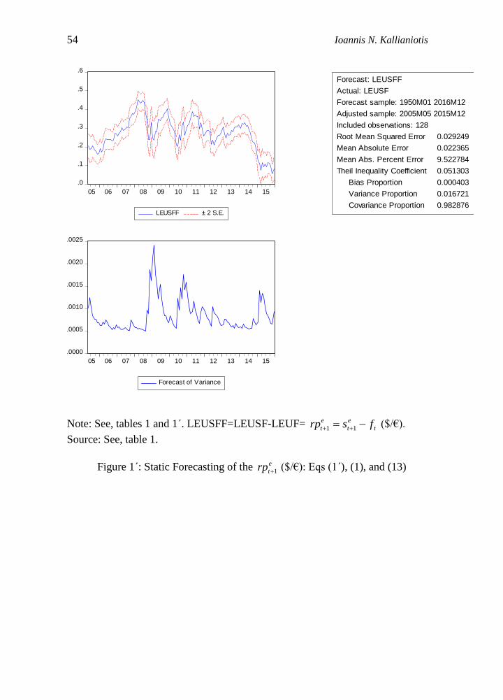
54 Ioannis N. Kallianiotis
.0
.1
.2
.3
.4
.5
.6
05 06 07 08 09 10 11 12 13 14 15
LEUSFF ± 2 S.E.
Forecast: LEUSFF
Actual: LEUSF
Forecast sample: 1950M01 2016M12
Adjusted sample: 2005M05 2015M12
Included observations: 128
Root Mean Squared Error 0.029249
Mean Absolute Error 0.022365
Mean Abs. Percent Error 9.522784
Theil Inequality Coefficient 0.051303
Bias Proportion 0.000403
Variance Proportion 0.016721
Covariance Proportion 0.982876
.0000
.0005
.0010
.0015
.0020
.0025
05 06 07 08 09 10 11 12 13 14 15
Forecast of Variance
Note: See, tables 1 and 1΄. LEUSFF=LEUSF-LEUF= t
e
t
e
t fsrp 11 ($/€).
Source: See, table 1.
Figure 1΄: Static Forecasting of the e
trp 1 ($/€): Eqs (1΄), (1), and (13)
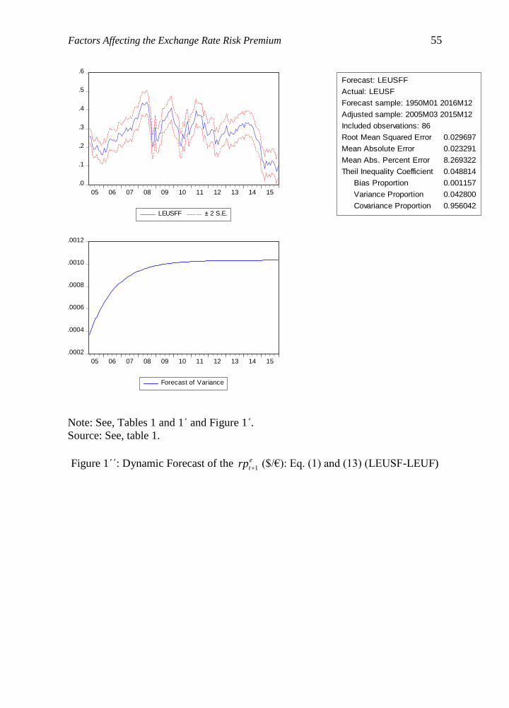
Factors Affecting the Exchange Rate Risk Premium 55
.0
.1
.2
.3
.4
.5
.6
05 06 07 08 09 10 11 12 13 14 15
LEUSFF ± 2 S.E.
Forecast: LEUSFF
Actual: LEUSF
Forecast sample: 1950M01 2016M12
Adjusted sample: 2005M03 2015M12
Included observations: 86
Root Mean Squared Error 0.029697
Mean Absolute Error 0.023291
Mean Abs. Percent Error 8.269322
Theil Inequality Coefficient 0.048814
Bias Proportion 0.001157
Variance Proportion 0.042800
Covariance Proportion 0.956042
.0002
.0004
.0006
.0008
.0010
.0012
05 06 07 08 09 10 11 12 13 14 15
Forecast of Variance
Note: See, Tables 1 and 1΄ and Figure 1΄.
Source: See, table 1.
Figure 1΄΄: Dynamic Forecast of the e
trp 1 ($/€): Eq. (1) and (13) (LEUSF-LEUF)