Factors Affecting Financial Performance of Agricultural Firms Listed on Shanghai Stock Exchange

Wei Wei

http://eprints.utcc.ac.th/id/eprint/1333    

 

 

© University of the Thai Chamber of Commerce

EPrints UTCC http://eprints.utcc.ac.th/

FACTORS AFFECTING FINANCIAL PERFORMANCE OF AGRICULTURAL FIRMS LISTED ON SHANGHAI STOCK EXCHANGE

MS. WEI WEI

A Thesis submitted in Partial Fulfillment of the Requirements

For the Degree of Master of Business Administration

Department of International Business

International College

University of the Thai Chamber of Commerce

2012

 

iv  

Thesis Title Factors Affecting Financial Performance of Agricultural Firms

Listed on Shanghai Stock Exchange

Name Wei Wei

Degree Master of Business Administration

Major Field International Business

Thesis Advisor Dr. Wanrapee Banchuenvijit

Graduate Year 2012

ABSTRACT

The research aims to examine the effect of liquidity, asset utilization, leverage,

economic prosperity and agricultural products price index on financial performance of

agricultural firms listed on Shanghai Stock Exchange (SSE) from 2006 until 2010. Due

to the non-stationary series data and multicolliearity problem that may result in a

spurious regressions, the Unit-Root test was used to check the stationary qualification

and Multicollinearity test was used to check the multicollinearity problem before the

regression results. The research found that the factors that effect on financial

performance of agricultural firms listed on SSE are asset utilization, leverage and

agricultural products price index.

v  

ACKNOWLEDGEMENTS

This thesis would have not been finished unless there were many sincere

supports. I hereby would like to express greatest gratitude to everyone who has

contribution to this fulfillment.

Firstly and most important, I am indebted to Dr. Wanrapee Banchuenvijit, my

advisor, her efforts and insights have a continuous source of inspiration in this study.

She often encouraged me to go ahead with my thesis whenever difficulties came and

without her the thesis would not have been completed.

Secondly, I also would like to thank other professors, Dr. Phusit Wonglorsaichon

who taught me how to do thesis step by step. Dr. Li Li and Assoc. Prof. Sriaroon

Resanond who provided many important comments and guidance for the thesis.

I would like to thank my entire friends in Bachelor Degree and Global MBA

program, both in the University of Thai Chamber of Commerce for their help, friendship

and moral support.

Most importantly, my deepest appreciation goes to my beloved family for their

kindness, attention, unconditional love, generous encouragement during the time of

troublesome.

vi  

TABLE OF CONTENTS

Page

ABSTRACT..................................................................................................................... iv

ACKNOWLEDGEMENT.................................................................................................. v

TABLE OF CONTENT.................................................................................................... vi

LIST OF TABLES........................................................................................................... ix

Chapter 1: Introduction

1.1 Background ...................................................................................................... 2

1.2 Statement of Problems .................................................................................... 3

1.3 Research Objectives ......................................................... ………….………… 6

1.4 Research Questions ...................................................................................... 6

1.5 Scope of the Study ......................................................................................... 7

1.6 Expected Benefits ........................................................................................... 7

1.7 Operation Defintions …. .................................................................................. 8

1.8 Organization of the Study ............................................................................. 10

Chapter 2: Literature Review

2.1 Financial Performance Evaluation .............................................................. 13

Page

vii  

TABLE OF CONTENTS (CONTINUED)

2.2 Firm Financial Performance ........................................................................ 17

2.3 Factors Affecting Financial Performance .................................................... 21

2.4 Conceptural Framework .............................................................................. 39

Chapter 3: Methodology

3.1 Research Design ......................................................................................... 42

3.2 Population ................................................................................................... 42

3.3 Variables of Research ................................................................................. 45

3.4 Data Collection ............................................................................................ 46

3.5 Data Analysis .............................................................................................. 48

3.6 Hypothesis ................................................................................................... 50

Chapter 4: Results of Analysis

4.1 Unit – Root Test .......................................................................................... 52

4.2 Descriptive Statistics ................................................................................... 53

4.3 Multicollinearity Test .................................................................................... 55

4.4 Regression Results ..................................................................................... 56

viii  

TABLE OF CONTENTS (CONTINUED)

Chapter 5: Conclusion, Discussion, and Recommendation

5.1 Conclusion ................................................................................................... 66

5.2 Discusssion ................................................................................................. 68

5.3 Implication of the Study .............................................................................. 72

5.4 Research Recommendation ........................................................................ 74

5.5 Limitations and Further Research ............................................................... 75

REFERENCES ................................................................................................................ 77

APPENDICES ................................................................................................................. 93

BIOGRAPHY ................................................................................................................. 117

Page

ix  

LIST OF TABLES

Table 3.1 Agricultural Firms Listed on Shanghai Stock Exchange List .......................... 44

Table 3.2 Data Source ..................................................................................................... 47

Table 4.1 The Results of Stationary Test by Unit – Root Test ....................................... 52

Table 4.2 Data Description .............................................................................................. 53

Table 4.3 The Correlation of the Independent Variables ................................................ 55

Table 4.4.1.1 Regression Results of ROA ...................................................................... 56

Table 4.4.1.2 Adjusting Regression Results of ROA ...................................................... 58

Table 4.4.2.1 Regression Results of ROS ...................................................................... 60

Table 4.4.3.1 Regression Results of SG ......................................................................... 61

Table 4.4.3.2 Adjusting Regression Results of SG ......................................................... 63

Table 5.1 Summarize for Testing Hypothesis ................................................................. 68

Page

CHAPTER 1

INTRODUCTION

The purpose of this chapter is to present the study of the importance of the

factors affecting the agricultural firms listed on Shanghai Stock Exchange. The following

are topics in this chapter:

1.1 Background

1.2 Statement of Problems

1.3 Research Objectives

1.4 Research Questions

1.5 Scope of the Study

1.6 Expected Benefits

1.7 Operational Definition

1.8 Organization of the Study

 

2    

1.1 Background

As the stock market of China has been developing 20 years, the listed firm has

become the leading role in the market economy stage. During these years, the number

of the listed firm has soared to more than one thousand from several at first. Investor’s

description and appraisal of asset management and utilization quality, debt risk and

credit capacity, profit ability and profit quality, and capital expanding and corporate

growth potential are directly reflected by the fluctuation of the return on assets and the

return on sales. Financial performance of listed firms becomes the issue of common

concern of the stakeholders including the shareholder, the creditor, the company staffs

and the government administration and so on. At present, as the capital market

expands and speeds, a great number of firms crowd into it. Although most listed firms

are excellent representative of their businesses, the working rule of market economy,

which is the competition mechanism of the superior winning and the inferior washing,

leads to the different financial performance, and some of the differences are even big.

Firm’s financial performance can reflect their development condition. Therefore, carrying

on the influencing factors of their financial performance has the extremely profound

theoretic and practical meaning of grasping the listed company’s development trend,

and seeking for the strategy of improving and the promoting their financial performance.

China is also a large agricultural nation, and rural population accounts for 75%

of the overall population. To adjusting the structure of agricultural production, to

strengthen the countryside infrastructural facilities and increase the rural labor force

employment, to increase the farmers’ income, has been one of the party and

3    

government’s work centers. Pushing agricultural firm to form an industry and certain

size, to grow strongly and greatly, and more leading ones to enter the market after the

joint stock transformation, are the important actions of solving the “Three Agriculture”

problem. However, Wang (2008) originally described the series of problems of low profit

capacity and property quality caused by the business’s own characteristics, weaknesses

as well as the management environment, have affected the listed firms’ sustained

development to a large degree. Thus, analyzing objectively and appraising the financial

performance condition of the agricultural listed firms, which is an important area which

relates to Chinese thriving and Chinese people’s surviving, discovering the primary

factors that influence the finance performance of agricultural listed firms, proposing

constructive policy to support the development of agricultural listed firms, is a vital

practical thing.

1.2 Statement of Problems

As a representative in the advanced agricultural production force in China,

listed agricultural firms are born and developed as the result of China’s development

and merge of market-oriented agriculture and capital market, which also reflects the

mutually benefited and promoted relationship between agriculture and securities market.

The birth and development of the listed agriculture firms is quite important to the

agricultural restructuring, industrialized management of agriculture, improving

agricultural products quality and agricultural management, upgrading international

competitiveness of agriculture and quickening the agricultural modernization in China.

4    

Wu et al. (2010), good financial performance is the precondition of agricultural listed

firms to be sustained and healthy development. Rising profitability is the driving force of

agricultural listed firms to drive agriculture from traditional agriculture to modern

agriculture. Therefore, the study on factors affecting financial performance of agricultural

listed firms helps firms to improve its financial performance and to maintain sustainably

growth.

However, in recent years, Peng (2006) mentioned that a series of problems

related to the transitional economic background and historical factors have led to the

poorer financial performance, higher risks of the listed agricultural firms, which have

consequently affected the competitiveness and sustained development of the firms. The

financial performance of the listed agricultural firms can reflect their development.

Therefore, the deep analysis of the factors affecting their financial performance in the

background of transitional economy in China is theoretically and practically vital to

understand the development trend of the listed agricultural firms and improving their

financial performance.

According to Gao (2010), agriculture is foundation of national economy. China

is a large agricultural country as well as a developing agriculture country. Agricultural

listed firms financed from capital market and promote agriculture integration operation,

which is a trend in the future of agriculture development. However, agricultural listed

firms have faced big challenge in China that financial performance is getting worse and

diversification operations are in failure from news and papers.

5    

As stated in Hao (2011), China has a large population, but has a relatively

small field land. As of 2010, China has field land area only about 300.796 million acres.

The per capita field land area is 0.227 acre, which only 40% of the world average. Thus

it can be seen the important to improve the productivity of the agricultural sector. The

agricultural economy is the foundation of the national economy, and agricultural listed

firms are also an important component of China’ stock market. Therefore, it’s very

necessary to study the factors affecting on financial performance of agricultural listed

firms.

Qin et al. (2011) showed that agricultural listed firms are essential on the

sustainable development of agriculture. The small population quantity, slow

development, weak growing capacity, relatively poor rationality and unbalanced regional

distribution situation of China’s agricultural listed firms have seriously restricted the

development of China’s agricultural economy.

The financial performance of agricultural firms changes over time. Profits are

different from one year to another and from one firm to another. Some firms obtain

increases in profit; others record decreases and some even losses. What are the

reasons of these changes and which are the factors of financial performance that

influences it to be different in time and space? This paper will try to answer these

questions.

1.3 Research Objectives

The research objectives are shown as follows:

6    

1. To examine the effects of liquidity on financial performance of agricultural

firms listed on Shanghai Stock Exchange.

2. To examine the effects of asset utilization on financial performance of

agricultural firms listed on Shanghai Stock Exchange.

3. To examine the effects of leverage on financial performance of agricultural

firms listed on Shanghai Stock Exchange.

4. To examine the effects of economic prosperity on financial performance of

agricultural firms listed on Shanghai Stock Exchange.

5. To examine the effects of agricultural products price index on financial

performance of agricultural firms listed on Shanghai Stock Exchange.

 

1.4 Research Questions

This study will attempt to answer the following research questions:

1. How does liquidity affect financial performance of agricultural firms listed on

Shanghai Stock Exchange?

2. How does asset utilization affect financial performance of agricultural firms

listed on Shanghai Stock Exchange?

3. How does leverage affect financial performance of agricultural firms listed on

Shanghai Stock Exchange?

4. How does economic prosperity affect financial performance of agricultural

firms listed on Shanghai Stock Exchange?

7    

5. How does agricultural products price index affect financial performance of

agricultural firms listed on Shanghai Stock Exchange?

1.5 Scope of the Study

This study intends to investigate factors that affect financial performance of

firms that focused only on the agricultural firms listed on Shanghai Stock Exchange.

Dependent variables of the study are return on assets, return on sales and sales

growth, and independent variables are liquidity, asset utilization, leverage, economic

prosperity and agricultural products price index. This study uses quarterly Financial

Statement data starting from January 2006 to December 2010.

1.6 Expected Benefits

These expected benefits of this study are shown as follows.

1. To examine factors that affect return on assets, return on sales and sales

growth, and increase ability to improve the financial performance of agricultural firms

listed on Shanghai Stock Exchange.

2. This study can also be used as resource information for future studies on

factors affecting firm’s financial performance.

8    

1.7 Operational Definition

Financial performance refers to the performance of how well a firm is using

its resource to make a profit, which is measured by return on assets, return on sales

and sales growth.

Return on assets (ROA) reveals the ability of the firm to create profit in excess

of actual uses from assets. The higher ROA; the more efficiently use its assets. The

ROA is calculated by:

ROA =Net  IncomeTotal  Assets

Return on sales (ROS), which is also known as net profit margin. It reveals the

efficiency of firm’s operation. It provides insight into how much profit is being earned per

unit of payment. It is better to compare this ratio with other firm in the industry to know

how well the firm can do. The higher ROS; the more profitability the firm gets. The ROS

is calculated by:

ROS =Net  IncomeNet  Sales

Sales growth (SG) reveals the ability of firm increasing the percentage of sales

between two quarters. The higher SG; the good sales be bringing by firm. The SG is

calculated by:

SG =Sales! − Sales!!!

Sales!!!×100%  

Liquidity is proxied by current ratio; calculate as current assets over current

liabilities.

Current ratio reveals how capable a firm is in paying its current liabilities by

using current assets only. The higher current ratio, the more liquid the firm has. The

current ratio is calculated by:

9    

Current  Ratio =Current  Assets

Current  Liabilities

Asset utilization is proxied by total asset turnover ratio; calculate as sales

over total assets.

Total asset turnover ratio reveals how effectively the firm uses its assets to

generate sales or revenues. The higher total asset turnover ratio, the more productively

the firm uses its assets. The total asset turnover ratio is calculated by:

Total  Asset  Turnover  Ratio =Sales

Total  Assets

Leverage is proxied by debt ratio; calculate as total debt over total assets.

This ratio represents the potential risks the firm faces in terms of its debt-load.

Debt ratio reveals the relation between the total debt, total equity and liabilities

of firm. The higher debt ratio, the higher level of liabilities that firm has. The debt ratio is

calculated by:

Debt  Ratio =Total  Liabilities

Total  Equity  and  Liabilities

Economic prosperity is proxied by gross domestic product (GDP). Chinese

GDP is the end results of the production activities of all the resident units (including

foreign firms) within China borders in a given period.

Agricultural products price index is proxied by the producer price index of

agricultural products in China. The producer price index of agricultural products is the

relative number of the change tendency and magnitude of the agricultural products

selling price in a certain period.

1.8 Organization of the Study

The study consists in five chapters as follows:

10    

Chapter1 Introduction

In the introduction, this chapter describes the background, statement of

problems, research objectives, research questions, scope of study, expected benefits,

operations definition and organization of the study.

Chapter2 Literature Review

This chapter presents the relevant theories to understand the related

conception, related research and conceptual framework to this study.

Chapter3 Methodology

This chapter includes research design, population and sample size, variable of

the research, data collection, data analysis and hypothesis.

Chapter4 Data Analysis and Results

This chapter includes Unit – Root test, descriptive statistics, multicollinearity

test and regression results.

Chapter5 Conclusion, Discussions and Recommendations

This chapter includes conclusion, discussion, implication of the study, research

recommendation and limitations and further research.

 

CHAPTER 2

LITERATURE REVIEW

This chapter represents review of the concept from the prior researches and

relevant literatures. The followings are topics in this chapter;

2.1 Financial Performance Evaluation

2.2 Firm Financial Performance

2.3 Determinants of Firms Performance

2.4 Conceptual Framework

 

13    

2.1 Financial Performance Evaluation

The financial performance evaluation is to carry out an evaluation and analysis

of the financial status of a company so as to reflect its financial situation and developing

trend on the basis of the financial indexes reflected in its financial statements. It

provides important financial information for the company to improve its financial

performance and decision-making process (Zhang, 2007).

Evaluation refers to the management of the object by using the corresponding

scientific method comparing results received with goal booked originally and therefore

obtains course of the best result (Kim and Takahiro, 1991). Financial performance

evaluation is a method of analysis and evaluation through the relevant data of

organization financial statements and other materials collecting calculating comparing

and explaining, and further reveals the financial position, profitability, operating

conditions (Suwignjo, Bititci and Carrie, 2000).

To evaluate a firm’s financial performance and condition, the financial analyst

needs to perform “checkups” on various aspects of a firm’s financial health. A tool

frequently used during these checkups is a financial ratio (James and John, 2005).

There are many papers used financial ratios to evaluate firm performance.

Beaver (1966) selected 79 companies from the crisis companies between 1954

and 1964. Beaver found that the best variable to explain company financial performance

is Cash Flow/Total Liabilities Ratio, followed by Total Liabilities/Total Assets Ratio, Net

14    

Profit/Total Assets Ratio, Working Capital/Total Assets Ratio, and Current

Assets/Current Liabilities Ratio.

Altman (1968) proposed the famous Z-Score model. He used 33 companies

declared bankruptcy in 1946-1965 as the research sample; and then selects 33 normal

companies to pair in accordance with the industry and size of the sample. Altman

chosen the 22 kinds of financial ratios; select five financial ratios have the most

explanatory capacity by stepwise multiple discriminate analysis method: Working

Capital/Total Assets, Retained Earnings/Total Assets, EBIT/Total Assets, Rights and

Interests of Market Value/Total Liabilities, Sales/Total Assets.

Altman (1977) modified the Z-Score model, proposed Zeta model. Empirical

results show that there are seven significant variables to test company performance:

Pretax Net Profit/Total Assets, 10-year Standard Error of Pretax Net Profit/Total Assets,

Pretax Net Profit/Interest Payments, Current Assets/Current Liabilities, Retained

Earnings/Total Assets, 5-year ordinary shares’ Average Total Market Value/Total Capital

and 5-year common stock Average Total Market Value/Total Size.

Ou (1990) studied that the nonprofit figures in the annual financial contain the

information of the next year earnings change direction. The dependent variable of his

design prediction model is the probability of next year’s report earnings will higher or

lower than the expected earnings (predicting based on time series model). About

predicting variables, he established a candidate set of variables consisting of 61

independent variables at first; and then selected 8 independent variables: the stock

divided by total assets ratio, total asset turnover ratio, the changes in the dividend per

15    

share (compared with the previous year), the growth rate of depreciation expense,

capital expenditures divided by total assets ratio, the prior year capital expenditures

divided by total assets ratio, ROE, the changes rate of ROE(compared with the previous

year).

Kloptchenko (1998) tested financial performance according to previous

researches selected 7 financial ratios: Operating Margin, Return on Total Assets, Return

on Equity, Current Ratio, Shareholders’ Equity Ratio, Interest Coverage Ratio, and

Accounts Receivable Turnover Ratio.

Chen (2000) discussed the prediction problem of ST companies in China’s

stock market through financial ratios derived from the annual report of listed companies.

He selected 6 financial ratios as explanatory variables: Current Ratio, Assets Liabilities

Ratio, Total Assets Turnover Rate, and Return on Total Assets, Return on Equity and

Return on Sales. As the cash flow information is impossible to completely obtain

(Chinese companies began cash flow statement in 1998), Chen Yu selected the

financial ratios are not involved in the cash flow ratios.

Wu and Lu (2001) studied how to establish models for examine financial

performance in China’s listed companies. They firstly selected 21 financial ratios, and

then use regression method to select 6 significantly financial ratios: Earnings Growth

Index, Return on Assets, Current Ratio, Long-Term Liabilities/Shareholders’ Equity

Ratio, Working Capital/Total Assets Ratio and Asset Turnover.

Lam (2004) tested financial performance and selected 16 financial statements

variables according to previous studies: Current Assets/Current Liabilities, Sales

16    

Income/Total Assets, Net Profit/Sales Revenue, Total Liabilities/Total Assets, Total

Sources of Funds/Total Use of Funds, R&D Expenses, Pre-tax Profit/Sales Revenue,

Current Assets/Common Equity, Outstanding Shares, Capital Expenditure, Earnings per

Share, Dividend per Share, Depreciation Expense, Deferred Tax and Investment Loan,

Common Stock Market Price, Relative Stock Price Index.

Zhang et al. (2006) chose the 15 financial ratios to examine the factors of

financial performance; there are net assets per share, dividend payout ratio, dividend

per share, ROA, retained earnings ratio, current ratio, quick ratio, debt ratio, long-term

debt ratio, receivable payment ratio, inventory turnover ratio, ROS, net profit margin,

return on investment and ROE.

Liu (2010) chosen 23 financial ratios to determine the financial performance

evaluation system, and used regression analysis and factor analysis to analyze the data

of 2008 China’s top 10 steel industry firms listed on Shanghai and Shenzhen stock

exchange. The results showed that the nine financial ratios are more relevant

relationship with financial performance mainly: asset-liability ratio, current ratio, total

asset turnover, current ratio, quick ratio, total assets profit margin, the main business

profit margin, the growth rate of main business income and net profit growth.

2.2 Firm Financial Performance

Domestic and foreign scholars already have a unified view on the definition of

the firm financial performance. In general, Shi Qi (2009) defined the firm financial

performance as the firm operating results within a certain period; it can be

17    

comprehensive reflection by the situation of profitability, asset quality, financial risk and

business growth conditions etc. Zhang (2010) defined the firm performance as the

results or outcomes of firm during a certain operating period; and defined financial

performance as the performance measured by using financial ratios. Firm financial

performance evaluation refers to the suitable and scientific evaluation for firm operating

effectiveness and operators’ performance by using financial ratios. Its definition is

related to the selection of financial ratios, ratios system establishment and the use of

what kind of evaluation method etc. Maryanee and Don (2006) defined return on assets

(ROA) as a measure how efficiently assets are used by calculating the return on total

assets uses to generate profit. James and John (2005) defined return on sales (ROS)

as the sum of net sales minus cost of goods sole divided by net sales. ROS shows that

the profit of the firm relative to sales, after deduct the cost of producing the goods. ROS

is a measure of the efficiency of the firm’s operations, as well as an indication of how

products are priced.

However, scholars have different view on the selection of firm financial

performance ratios. The early scholars focused on return on shareholders’ mainly based

on the capital market transactions data, such as the empirical test of Moskowitz (1975)

and Vance (1975) were based on market income ratios to measure the firm’s financial

performance. But Bowmen (1978) proposed should be based on financial statements

data, and selects the accounting ratios to reflect the operating results of the entire firm;

the accounting ratios include the return on assets (ROA), return on equity (ROE) and

earnings per share (EPS) etc. In the 1980s, there are many scholars evaluated the

whole firm financial performance by using market ratios and accounting ratios. McGuire

18    

et al. (1988) selected the market return ratios and the accounting ratios to measure the

firm’s financial performance; the market return ratios include the total market return and

risk-adjusted market return etc.; the accounting ratios include return on assets (ROA),

total assets, sales growth, asset growth and operating profit growth etc. In a word,

accounting ratios capture only historical aspects of firm performance (McGuire,

Schneeweis and Hill, 1988). They are subject, moreover, to bias from managerial

manipulation and differences in accounting ratios measuring procedures (Branch, 1983;

Brilloff, 1972). There are many financial ratio related researches focused on the ability

of financial statement related ratios to study the financial performance (Beaver, 1966,

1968; Altman et al., 1977; Ambrose and Seward, 1988; McNamara et al., 1988).

Schmalensee (1985) empirical analyst what’s the reasons of the performance

differences of firms in the same industry. Return on assets was measured as the ratio

of firm performance to research factors affecting on firm performance (firm’s

profitability).

Stigney (1990) stated return on assets was measured by the earnings before

interest, tax and extraordinary items, divided by net tangible assets in financial

performance analysis.

Ray and Keith (1995) argued for the rate of return on assets was measured as

the best decomposition of financial ratios for the purposes of studying financial

performance.

According to Waddock and Graves (1997) used return on assets (ROA), return

on equity (ROE) and return on sales (ROS) these three accounting ratios to measure

19    

firm financial performance; and chose firm size, risk and industry as control variables on

studying the determinant of firm financial performance.

Return on assets (ROA) is a widely used measure of financial performance

(Barry et al., 1995) that can be influenced by many aspects of the agricultural firms.

Ruf et al. (2001) chose return on equity (ROE), return on sales (ROS) and

growth in sales to measure firm financial performance in the research on the

determinants of financial performance by analytic hierarchy process.

Regressions were used on the panel data for the 422 firms for year 1996 to

year 2000. The financial performance was measured by return on assets (ROA), return

on equity (ROE) and return on sales (ROS) to study the relationship between corporate

social responsibility and financial performance (Margarita, 2004).

Hitt et al. (2006), return on assets is the ratio to measure firm performance, to

be operationalized as the ratio of operative income to total assets. Claudio (2012)

collected data of 48 Italian facility management firms from between 2000 and 2009 to

study firm performance by using return on assets (ROA) as the dependent variable to

measure firm financial performance.

Gerwin, Hans and Arjen (2007), Firm financial performance information is

obtained from Thomson Financials DataStream. They used return on assets (ROA) and

earnings per share (EPS) to research financial performance of the S&P 500 in the

1997-2002 periods.

20    

Chen (2008) suggested return on assets is a highly comprehensive and the

most representative financial ratio; comprehensively reflects the scale of sales, cost

control and capital operation of firm; and reflects the results of firm’s business activities

and the goal of maximizing value of the firm to pursue.

Guan, Qiu and Zhang (2009) analyzed the external factors affecting business

performance by selecting the return on assets as an indicator to measure firm

performance; and pointed out return on assets (ROA) can better reflect the financial

position and profitability.

Peters and Mullen (2009) studied the determinant of financial performance of

81 firms in the U.S. Fortune 500 firms by using return on assets to measure firm

financial performance.

Zeng et al. (2009) used regression method to examine the relationships

between ten business factors and firm financial performance (return on assets to be

measure) of Chinese manufacturing.

Fu (2011) researched on the relationship between corporate social

responsibility and financial performance from the general stakeholder perspective and

separate stakeholder dimension perspective. He used return on assets to measure long-

term firm performance and used Tobin-Q to measure long-term firm performance.

Yang (2011) present return on assets is the ratio of net income and total

assets. It reflects the ability of return on capital; and reflects the management total

assets level of listed firms and the condition of reasonably used. The higher operational

efficiency of the firm’s total assets, the better financial performance firm has.

21    

2.3 Factors Affecting Financial Performance

Many researchers have done the research about factors affecting firm financial

performance. Since the establishment of modern firm’s system, the experts and

scholars pay more attention on the financial performance and the factors of financial

performance. According to previous studies, this study discuss about each independent

variable that may affect firm financial performance, including liquidity, asset utilization,

leverage, economic prosperity and agricultural products price index.

2.3.1 Liquidity

2.3.1.1 The general concept of liquidity ratios

According to James and John (2005), liquidity ratios are defined as a measure

of a firm’s ability to pay back short-term obligations. Much insight can be obtained into

the present cash solvency of the firm and the firm’s ability to remain solvent in the event

of adversity. Liquidity ratios can be measure by current ratio and quick ratio. Steve et al.

(2006) defined current ratio as a measure of an entity’s liquidity. Current ratio equal

current assets divide by current liabilities. The higher the current ratio, the greater ability

of the firm pays its bills. High current ratios would appear to be good (if you are a

creditor of a firm, a high current ratio indicates that you are more likely to be paid); a

ratio that is very high may indicate that a company holds too much cash, accounts

receivable, or inventory. High levels of accounts receivable may indicate problems

collecting cash from customers, and cash held in noninterest-bearing accounts might be

22    

more productively used elsewhere. Maryanne and Don (2006) defined quick ratio as a

measure of liquidity that compares only the most liquid assets to current liabilities. Quick

ratio equal to quick assets divides by current liabilities. The quick ratio is a stricter test

of a firm’s ability to pay its current debts with highly liquid current assets. The quick

ratio removes inventories and prepaid assets from the current asset amount used in the

calculation of the current ratio.

2.3.1.2 Liquidity and financial performance

Adams and Buckle (2003) was defined as current assets over current liabilities.

Their study pointed out that liquidity measures the ability of managers in firms to fulfill

their immediate commitments to policyholders and other creditors without having to

increase profits on underwriting and investment activities and liquidate financial assets.

Liquidity was statistically significant at the 0.01 level in a one tail test. It found that

liquidity was positively related to financial performance.

Fazzari et al. (1988) collected the data of 421 U.S. manufacturing firms in the

period 1970-1984. The results showed that the level of liquidity has a significant impact

on firm performance. Hu et al. (2006) studied the data of China’s listed firms and found

that liquidity has a significant positive correlation to firm performance.

Jose et al. (2010) examined the relative efficiency of 11 major Chinese ports

by using an innovative adopted version of Data Envelopment Analysis based on

financial ratios in which no inputs are utilized. He used liquidity (current ratio and quick

23    

ratio) to analysis the efficiency of each port. A high current ratio and quick ratio indicate

that the firm is liquid, and has the ability to meet its current or liquid liabilities in time,

while a low current ratio and quick ratio indicate the firm’s liquidity position is not in a

good condition.

Seema et al. (2011) measured the factors impact on the performance of

central public sector enterprises (PSEs) over a period of time (1994-1995 to 2006-

2007). Liquidity has been assessed by current ratio (CR) and acid test ratio (ATR). CR

takes into account five items of current assets, i.e. sundry debtors, loans and advances,

cash and bank balances, inventories and stock of other current assets. The findings

showed the increase in liquidity has brought salutary impact on the financial

performance of firms.

Sibel and Engin (2012) analyzed financial performance on selected financial

ratios and its effect on macroeconomic variables for real estate investment trust firms

which are indexed on Istanbul stock exchange (ISE). The liquidity ratios have significant

relation on financial performance of the real estate investment trusts on ISE.

2.3.2 Asset Utilization

2.3.2.1 The general concept of asset utilization ratios

As the stated in Stephen et al. (2010), asset utilization ratios are intended to

describe is how efficiently or intensively a firm uses its assets to generate sales. Asset

utilization ratios can be measured by total assets turnover ratio, accounts receivable

turnover ratio inventory ratio and fixed asset ratio. Total assets turnover ratio (capital

24    

turnover ratio) is measuring relative efficiency of total assets to generate sales. An

increase in the firm’s total asset turnover increases the sales generated for each dollar

in assets. This decrease the firm’s need for new assets as sales grow and thereby

increases the sustainable growth rate. Increasing total asset turnover is the same thing

as decreasing capital intensity. Maryanne and Don (2006) defined accounts receivable

turnover ratio as net sales divided by average accounts receivable. The inventory

turnover ratio is computed by dividing the cost of goods sold by the average inventory.

A low turnover ratio may signal the presence of too much inventory or sluggish sales.

With fixed asset turnover ratio, it probably makes more sense to say that for every

dollar in fixed assets.

2.3.2.2 Asset utilization and financial performance

Jose et al. (2010) defined total asset turnover as the ratio measure the

efficiency of a firm to get incomes or revenues by using its assets. This ratio also

indicates pricing strategy. Businesses with low profit margins tend to have a high asset

turnover, and those with high profit margins tend to have a low asset turnover.

Wu, Li and Zhu (2010) pointed out total asset turnover ratio can reflect the

firm’s asset management. They empirical analysis the impact factors of firm

performance of agricultural listed firms by multiple linear regression model. The results

shown that return on assets and total asset turnover of agricultural listed firms are

significantly positively related. The asset turnover is essential for agricultural listed firms,

and directly impact on the ability and speed of firm to increase revenue and expand the

25    

scale. The ability of agricultural listed firms’ asset utilization made a great contribution to

the level of firm’s profitability, and had a significant effect on the firm’s financial

performance.

Ding and Sha (2011) collected the data of Jilin Forest Industry Co., Ltd to

study asset utilization affecting on firm’s financial performance by using principal

component analysis and multiple linear regression analysis. The results showed that

total asset turnover ratio is positively correlated with financial performance. The faster

firm’s total asset turnover, the higher efficiency of asset utilization and the better

performance the firm has.

According to Seema et al. (2011), asset utilization was included as total assets

turnover ratio (TATR), fixed assets turnover ratio (FATR) and current assets turnover

ratio (CATR). The lower turnover is indicative of under-utilization of available resources

and presence of idle capacity. Normally, the higher the firm’s total turnover ratio is, the

more efficiently are the assets being used. And the results found that the increase in

asset utilization ratios is commendable in firm’s financial performance.

2.3.3 Leverage

2.3.3.1 The general concept of leverage ratios

According to Stephen et al. (2010), leverage ratios are intended to address the

firm’s long-term ability to meet its obligations. When a firm has debt, it has the

obligation to repay the interest. Holding debt will increase the firm’s riskiness. Debt

carries with it the threat of default foreclosure and bankruptcy if income does not meet

26    

projections. Leverage ratios can help an individual evaluate a firm’s debt-carrying ability.

Leverage ratios can measure by debt ratio, debt to equity ratio. As stated in Maryanne

and Don (2006), debt ratio was defined as a measure the percentage of assets

financed by creditors’ increases, the riskiness of the firm increases. It is computed by

dividing a company’s total liabilities by its total assets. As the total liabilities are

compared with the total assets, debt ratio is measuring the level of protection afforded

creditors in case of insolvency. Creditors often impose restrictions on the percentage of

liabilities allowed. If this percentage is exceeded, the firm is in default. The debt to

equity is comparing the amount of debt that is financed by stockholders. Debt to equity

ratio equal to total liabilities divided by total stockholders’ equity. Creditors would like

debt to equity ratio to be relatively low, indicating that stockholders have financed most

of the assets of the firm. This ratio is higher, indicating that the firm is more highly

leveraged and stockholders can reap the return of the creditors’ financing.

2.3.3.2 Leverage and financial performance

The level of financial leverage shows the ability of listed firm to manage their

economic exposure to unexpected losses (Adams and Buckle, 2003). Sun (2011)

pointed out that capital structure refers to the composition ratio of each types of capital

in the total firm capital. Capital structure of a firm is an important factor affecting

financial performance (Ram et al, 1996). Recent advances in theories of finance

recognize capital structure of firm to be relevant for determining its financial

performance (Ram et al., 2003). Chen (2008) mentioned capital structure refers to the

27    

composition of all firm’s capital and the proportion of each capital. Debt ratio defined as

a measure ratio of firm financial leverage (Lu and Beamish, 2004).

There are many experts and scholars have done the related topic to research

leverage and firm financial performance, but didn’t get a consistent answer.

(1) Leverage and firm financial performance are positive correlated.

According to Masulis and Ronald W. (1980) studied to show that a positive

correlation between common stock price and firm financial leverage, and firm financial

performance is positively correlated with debt levels. Comett and Travlos (1989)

empirical results shown that financial leverage has a positive correlation with firm value,

the reason is that financial leverage and firm value as the endogenous variables will

occur in the same direction changes when effecting by the exogenous variables

changing. K. Shah (1994) observed the stock price was rising with the increase of the

firm’s financial leverage, and vice versa.

Wang and Yang (1998) researched the relationship among financing structure,

firm size and profitability of 461 firms listed on Shanghai Stock Exchange; and found

that these three ratios have positive relationship. Hong and Shen (2002) investigated

the data of 221 firms listed on Shanghai Stock Exchange from 1995 to 1997; and

concluded firm’s capital structure and financial performance have a positive correlation.

Wang and Yang (2002) used 845 firms listed on Shanghai and Shenzhen

stock exchange as the sample, capital structure (debt ratio) as being the explanatory

variable, and profitability (return on assets) as being the explaining variable, analyzed

28    

the relationship between these two variables by regression model based on 1999-2000

data, and found that capital structure and profitability have a positive correlation.

According to Yao and Chen (2008), capital structure and firm financial

performance of Chinese media listed firms have a positive correlation by constructing

panel data model. Li and Yang (2010) collected the panel data of 38 SME board listed

firms, found there was a positive correlation between debt ratio and financial

performance.

Zhang (2010) took the firms listed in SME board as research samples to study

the factors effecting on firm performance. The results shown debt ratio and firm

performance are positively related. Debt financing has leverage can bring a tax-

sheltered benefit; improve firm governance and firm performance.

Ding and Sha (2011) selected Jilin Forest Industry Co., Ltd as a research

objective, and studied the capital structure influence on firm’s financial performance by

using principal component analysis and multiple linear regression analysis. The

empirical results show that capital structure is positively correlated with financial

performance. Debt can bring a lot of the tax-shield benefits for firm. Increasing the firm’s

debt will help improve firm performance.

(2) Leverage and firm financial performance are negative correlated.

According to Titman and Wessels (1988) collected 1972-1982 panel data of

469 U.S. listed firms in the manufacturing sector, found a negative correlation between

profitability and debt ratio. Rajan and Zingalas (1995) found that, there was a negative

29    

relationship between profitability and firm performance, and this relationship continues to

strengthen with the increasing of the size of the firm.

Hall, Hutchin et al. (2000) studied the impact of long-term debt ratio on

profitability and the impact of short-term debt ratio on profitability. The results explored

short-term debt ratio has a negative relation with firm financial performance. Booth

(2001) compared 10 firms in developing countries as sample, and found that there were

negative correlation between capital structure and firm performance of the nine

countries (except Zimbabwe). Ram et al. (2003) collected financial statement and capital

market data of 566 large Indian firms to study Indian firms’ financial performance. They

found that capital structure in the form of the firm’s leverage had a negative relation with

financial performance, and the leverage of the firm was important factors affecting

financial performance. The negative relation of financial performance with leverage

could be expected on the fact that increases in debt leads to an increasing in the firm’s

financial and bankruptcy risk.

According to the research of Lu and Xin (1998), there was a negative

correlation between financial performance and capital structure (long-term debt ratio) of

35 machinery and transport equipment industry firms listed on Shanghai Stock

Exchange by using multiple linear regression models. Feng et al. (2002) explored

leverage and long-term debt ratio have a negative correlation with financial performance

of 234 issued A shares firms listed on Shanghai and Shenzhen stock exchange before

1995.

30    

Xiao (2005) established simultaneous equations of capital structure and firm

performance, and applied least-square method to expand existing researches. The

empirical results shown that: Capital structure (debt ratio) and firm performance (return

on assets) have apparent interactive relationship; financial leverage is negatively related

to firm performance.

Zhang, He and Liang (2007) used the data of 1,116 firms listed on Shanghai

and Shenzhen stock exchange from 2000 to 2004 (among them, 829 state-holding

firms, and 287 private firms). The results explored that debt ratio has negatively related

to the financial performance of all sample firms. The effect of debt ratio on the financial

performance of state-holding firms is better than the effect on the private firms.

Chen (2008) empirical analyzed the relationship between capital structure and

firm performance of 185 firms listed in SME board of Shenzhen stock exchange by

using regression analysis method, explored that, return on assets and debt ratio were

negatively correlated. It also meant reducing the debt ratio will improve return on assets

of firm.

Mo (2008) calculated the profitability comprehensive score of real estate

industry firms by using principal component analysis. Capital structure (debt ratio) has a

negatively correlation with financial performance (profitability).

According to Wu, Li and Zhu (2010), Chinese listed firms prefer equity

financing, but foreign firms prefer debt financing because of capital structure theory

point out the cost of debt financing is lower. They collected data of 42 Chinese

agricultural listed firms, and found that return on assets and debt ratio has a significant

31    

negatively related. It explained capital structure of high debt is not suitable for the

development of financial performance of Chinese agricultural listed firms.

In conclusion, it has not yet conclusive about the relationship between

leverage and firm financial performance whether it is positively or negatively correlated,

because of the differences in study samples, firm performance ratios and research

methods.

2.3.4 Economic Prosperity

2.3.4.1 The general concept of economic prosperity

Gross domestic product (GDP) is defined as the sum of the money values of

all final goods and services produced in the domestic economy and sold on organized

markets during a specified period of time, usually a year (William and Alan, 2001).

According to Mankiw (2007), GDP (which we denote as Y) is divided into four

components: consumption (C), investment (I), government purchases (G), and net

exports (NX): Y = C + I + G + NX.

Ma (2011) defined gross domestic product (GDP) as measure of the economy

of the total production and services. GDP reflects a degree of national prosperity. When

there is a higher GDP, the economy is in boom, and the firms will have a higher level of

profitability. The result showed that GDP has a positively related to firm performance. A

large of researches has used GDP as proxy for overall economic prosperity. Real GDP

growth therefore represents changes in overall economic prosperity condition (Bikker &

32    

Hu, 2002; Athanasoglou et al., 2008; Chen, 2010). Economic power (GDP) has shifted

to the firm’s financial performance (Margarita, 2004).

2.3.4.2 Economic prosperity and financial performance

Ray and Keith (1995) stated the financial performance was determined by an

interaction of a number of factors. Return on assets was measured of base firm

performance and correlated with gross domestic product (the output factor). It would

seem that increases in the level of economic activity, as measured by GDP, are

accompanied by increases in ROA. The results found that GDP was positively affected

on ROA.

The empirical research of Deng et al. (2009) pointed out that firm performance

not only affects by the internal factors, but also affects by the macroeconomic

environment. They utilized the data of agricultural listed firms to study GDP, inflation

and interest rates etc. have influence on the firm performance. GDP is the most general

indicator that reflects the country’s overall macroeconomic situation. The fluctuation of

GDP reflects the situation of economic cyclical fluctuation. When the higher rate of GDP

growth, the economic is boom and the level of profitability is high, and the firm

performance is better. On the contrary, when the slowdown in GDP growth rate, the

actual level and the expected level of firm earnings will be reduced, and the firm

performance is bad. The results showed GDP was positively affecting on firm

performance.

33    

Yu et al. (2009) utilized the unbalanced panel data of 1174 firms listed on

Shanghai and Shenzhen stock exchange between the years 1994-2006. It analyzed the

factors affecting the firm performance in the background of economic reforming; and

found that GDP is significant and positively affecting on firm performance.

Chen (2010) observed the effects of the real GDP growth rate and the growth

rate of total foreign tourist arrivals on the mutual performance of tourist hotels are then

examined via panel regression tests. The results proved that both the real GDP growth

rate and the growth rate of total foreign tourist arrivals are significant explanatory factor

of occupancy rate; and can strongly explain return on assets (ROA) and return on

equity (ROS).

Zhang et al. (2010) investigated the firm performance of state-owned

enterprises (SOEs) listed on China’s two exchanges upon share issuing privatization

(SIP) in the period 1999-2005, and analyst determinants of firm performance from the

angles of macro and micro aspects. The results showed that GDP was positively

associated with firm performance.

John and Riyas (2011) suggested that Africa’s performance in sports was

dependent on a range of socio-economic factors. The results confirmed GDP was being

positively and significantly associated with better performance.

Ma (2011) focused on the macroeconomic factors influencing the firm

performance of agricultural listed firms. F-value of GDP was higher than other factors

(inflation etc.) to show that GDP had a high ability to explain the firm performance. GDP

had a significant relationship with firm performance.

34    

Engin, Ahmet and Metin (2011) analyzed the effects of macroeconomic

conditions and financial ratios on debt ratio and return on equity ratio of the tourism

firms. They selected six lodging company financial ratios that included tourism sector

index on Istanbul Stock Exchange between the years 2002-2010. According to the

results, firm performance (ROE) was positively affected by GDP.

Sibel and Engin (2012) estimated the impact of economic conditions and real

estate investment trusts’ development on financial performance of such firms in terms

of, not only their profitability, but also their overall financial performance as well. Results

indicated that firm financial performance has meaningful effect by GDP.

2.3.5 Agricultural Products Price Index

2.3.5.1 The general concept of agricultural products price index

Selcuk (2011) defined consumer price index (CPI) as a measure of average

prices for a basket of goods commonly bought by consumers. CPI is used for

determining whether general prices are higher, lower or stable over time, calculating

annual rate of inflation, and converting nominal values to real. The producer price index

(PPI) was defined as a measure of the average prices for a basket of inputs commonly

bought by producers. The PPI has two main functions: 1) to provide price index for use

in the deflation of gross domestic product (GDP) data; and 2) to provide a general

measure of inflation. In the past, PPI was often called “wholesale price index” (WPI).

WPI focuses on the prices of traded goods and services between corporations, rather

than goods and services bought by consumers. Producer prices of firm products

35    

increasing will leads to prices for intermediate products increasing, producer prices of

finished goods increasing and consumer prices increasing. These cause income of firm

increasing and the firm performance is good. Consequently, consumer prices can affect

producer prices.

Consumer price index (CPI) defined as a weighted average of the prices of a

fixed basket of goods and services purchased by a typical urban household (Jacueline

and Janna, 1999). The consumer price index (CPI) is when referring to the cost of

living, and only telling how prices in one year compare with those in another year.

Inflation refers to a sustained increase in the level of general price (William and Alan,

2001).The inflation calculation is taken the consumer price index of one year and

subtract the consumer price index for the prior year, then divide the answer by the

consumer price index for the earlier year(Jacueline and Janna, 1999).

The agricultural producer prices is the actual unit price be obtained by

agricultural producers directly selling their products. The agricultural producer price

index is reflecting the relative number between the trending and degree of agricultural

producer prices changing in a certain period (zhu, 2000). The agricultural producer price

index is a certain period series that measures the changes in prices that agricultural

producer receive from the agriculture commodities them producing and selling (Andy,

2001).

Lei (2003) pointed out that the agricultural producer price index is the price

index of agricultural products including the four larger categories of planting products,

forestry products, livestock products and fisheries products; the fifteen middle categories

36    

of grains, cotton, oilseeds, sugar, vegetables, horticulture, fruits, herbal medicines,

forest products, livestock, poultry, eggs, dairy products, marine products and fresh

products; and thirty small categories.

2.3.5.2 Agricultural products price index and financial performance

In the study of inflation (consumer price index), Demirguc-Kunt and

Maksimovic (1999) divided debt structure into long-term liabilities and short-term

liabilities and collected data of 30 countries (including 19 developed countries and 11

developing countries). The results showed that inflation (measured by consumer price

index) was negative correlation with long-term liabilities. High inflation causes low debt

level and good firm performance.

Booth et al. (2001) empirical researched on 10 developing countries and 7

developed countries and results showed that high inflation rate (measured by consumer

price index) will makes the firm debt level decreasing. It meant firm liabilities based on

actual economic growth rather than nominal economic growth. Although inflation makes

the monetary value of firm assets rising, but the high interest rate and currency risks

caused by high inflation will make firm liabilities decreasing. And the firm performance

will be better by high inflation.

As stated in Deng et al. (2009), for listed firms, sustained and stable inflation

(measured by consumer price index) will cause the firm’s actual wealth from the

creditors transferred to the shareholders. Inflation or the fluctuation of price affects firm

performance on: price fluctuations improve firm’s business risks and the possibility of

37    

firm losing tax. In an uncertain environment, when the debt financing is more than a

certain limit, the tax associated with the debt will become highly uncertain. Losing more

tax will reduce the benefits of shareholder get from debt financing. Shareholders will

tend to reduce financial leverage ratio; and it will affects firm performance. The results

showed that consumer price index is the factor affecting firm performance.

Wu (2011) proposed the agricultural products price index rising will radiate to

the consumer price index through the changes in agricultural products price. Agricultural

products, especially food products have a less elasticity of demand. It means that

residents increase the food consumption when agricultural products price increasing.

Then Engel’s coefficient will rise. In general, the Engel’s coefficient has a positive

relationship with the consumer price index. The agricultural products price increasing

will lead to the agricultural prices increasing, and then will bring the inflation pressures.

The inflation pressure will stimulate the general price level rising.

According to Ma (2011), consumer price index (CPI) affects the firm financial

performance in the following aspects: 1) price fluctuation leads to fluctuations in the

product price and cost structure of firm; leads to increase the volatility of the firm’s

revenue and improve the firm’s business risk; and leads to firm performance; 2) price

fluctuation makes the firms are uncertain the expected cash flows in the investment

project. The firms will use a higher discount rate when assessing the project. It will

result in fewer project has been adopted and the growth of firm, and can even affect the

firm performance. Ma researched how the CPI influences the firm performance of

agricultural listed firms; and found CPI can explain the firm performance, but has a

weak influence.

38    

2.4 Conceptual Framework

Based on the above literature review and according to the objective of the

study, the financial performance has been identified as dependent variable, liquidity,

asset utilization, leverage, economic prosperity and agricultural products price index as

independent variables. Thus, the conceptual framework is developing to study factors

affecting financial performance of agricultural companies listed on Shanghai Stock

Exchange as conceptual framework can be shown in figure 2.1.

39    

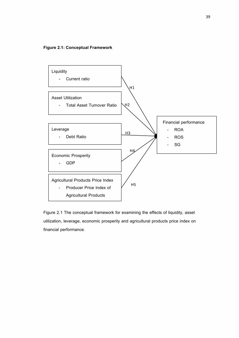
Figure 2.1: Conceptual Framework

Figure 2.1 The conceptual framework for examining the effects of liquidity, asset

utilization, leverage, economic prosperity and agricultural products price index on

financial performance.  

Financial performance - ROA - ROS - SG

Liquidity - Current ratio

Asset Utilization - Total Asset Turnover Ratio

Economic Prosperity - GDP

Leverage - Debt Ratio

Agricultural Products Price Index - Producer Price Index of

Agricultural Products

H1  

H4  

H3  

H2  

H5  

CHAPTER 3

RESEARCH METHODOLOGY

The purpose of this chapter is to present the methodology of collecting and

interpreting data of this study. The following are topics in this chapter;

3.1 Research design

3.2 Population

3.3 Variables of Research

3.4 Data Collection

3.5 Data Analysis

3.6 Hypothesis

42    

3.1 Research design

This study investigates and examines the effects of liquidity, asset utilization,

leverage, economic prosperity and agricultural products price index on financial

performance of agricultural firms listed on Shanghai Stock Exchange. Therefore, the

research is designed to use the quantitative research method and collecting the

secondary data by the financial information. The financial information is collected from

the quarterly financial reports, which includes balance sheets, income statements of

each agricultural firm listed on Shanghai Stock Exchange. This study is important since

it allows us to make a preliminary identification of factors that affect the dependent

variable of interest. It also allows us to identify variables that should be investigated

further.

This research use multiple regression analysis to examine factors that affect

the financial performance of agricultural firms listed on Shanghai Stock Exchange.

3.2 Population

This research samples come from the Shanghai Stock Exchange website.

There are 20 agricultural firms listed on Shanghai Stock Exchange. The analysis

periods in this paper are from 2006 to 2010, so China Hainan Rubber Industry Group

Co., Ltd (601118.SH) is excluded because it was listed in 2011. Further analysis of the

remaining 19 agricultural listed firms; some firms are marked as special treatment, so

this study will remove all those firms, which are Shangdong Jiufa Edible Fungus Co.,

43    

Ltd (600180.SH), Hubei Wuchangyu Co., Ltd (600275.SH), Zhongken Agricultural

Resource Development Co., Ltd (600313.SH) and Xinjiang Korla Pear Co., Ltd

(600506.SH). Therefore, this study includes 15 agricultural listed firms as shows in table

3.1.

Table3.1 Agricultural firms listed on Shanghai Stock Exchange List

NO. Code Firm’s Full Name Firm’s

Short Name

1 600097 Shanghai Kaichuang Marine International Co., Ltd KCGJ

2 600108 Gansu Yasheng Industrial (Group) Co., Ltd YSJT

3 600189 Jilin Forest Industry Co., Ltd JLSG

4 600242 Zhongchang Marine Co., Ltd ZCHY

5 600257 Duhu Aquaculture Co., Ltd DHGF

6 600265 Yunnan Jinggu Forestry Co., Ltd YJFC

7 600354 Gnsu Dunhuang Seed Co., Ltd DHZY

8 600359 Xinjiang Talimu Agricultural Development Co., Ltd XTAD

9 600371 Wanxiang Doneed Co., Ltd WXDN

10 600467 Shangdong Homey Aquatic Development Co., Ltd HDJ

11 600540 Xinjiang Sayram Modern Agriculture CO., Ltd XSGF

12 600598 Heilongjiang Agriculture Co., Ltd HACL

13 600962 SDIC Zhonglu Fruit Juice Co. Ltd SDICZL

14 600965 Fortune Ng Fung Food (Hebei) Co., Ltd FCWF

15 600975 Hunan New Wellfull Co., Ltd NWF

Source：Shanghai Stock Exchange Website

44    

3.3 Variables of Research

Based on the literature review and research journals, the following variables

are used for the research:

3.3.1Dependent variables

The dependent variables in this research are as following:

1. Return on assets (ROA)

2. Return on sales (ROS)

3. Sales Growth (SG)

3.3.2 Independent` variables

The independent variables in this research are as below:

1. Liquidity as proxied by current ratio.

According to Adams and Buckle (2003), James and John (2005), Sibel and

Engin (2012), current ratio was measured as liquidity to study the correlation with firm

financial performance. Maryanne and Don (2006) used quick ratio to measure as

liquidity. And Jose et al. (2010) used current ratio and quick ratio to measure as

liquidity. Seema et al. (2011) used current ratio and acid test ratio to measure liquidity.

2. Asset turnover as proxied by total asset turnover ratio.

As the stated in the studied of Jose et al. (2010), Wu et al. (2010), Ding and

Sha (2011), total assets turnover ratio was measured as asset utilization to study the

correlation with firm financial performance. And the research of Seema et al. (2011)

used total asset turnover ratio, fixed asset turnover ratio and current assets turnover

45    

ratio to measure as asset utilization.

3. Leverage as proxied by debt ratio.

As the stated in the studied of Titman and Wessels (1988), Xiao (2005), Zhang

et al. (2007) and Chen (2008), debt ratio was measured as leverage to study the

correlation with firm financial performance.

4. Economic prosperity as proxied by GDP,

5. Agricultural products price index as producer price index of agricultural

3.4 Data Collection

For the objective of this study, all data start from January 2006 until December

2010, totally 20 quarters and is used as a method for data collection. In the study

collected the data as much as possible. These data include: return on assets (ROA),

return on sales (ROS), sales growth (SG), current ratio, total asset turnover ratio, debt

ratio, gross domestic product (GDP) and agricultural products price index. These data

are collected from source as following:

46    

Table3.2 Data Source

Data Source

ROA Shanghai Stock Exchange (SSE);

Each listed firm’s website

ROS Shanghai Stock Exchange (SSE);

Each listed firm’s website

Sales Growth Shanghai Stock Exchange (SSE);

Each listed firm’s website

Current Ratio Shanghai Stock Exchange (SSE);

Each listed firm’s website

Total Asset Turnover Ratio Shanghai Stock Exchange (SSE);

Each listed firm’s website

Debt Ratio Shanghai Stock Exchange (SSE);

Each listed firm’s website

GDP National Bureau of Statistics of China

Agricultural Products Price Index National Bureau of Statistics of China

3.5 Data Analysis

This research will use regression analysis to investigate each factor affect the

financial performance of agricultural firms listed on Shanghai Stock Exchange. This

research will use data of these fifteen agricultural listed firms that includes current ratio,

47    

total asset turnover ratio, debt ratio, GDP and producer price index of agricultural

products.

Multiple regression analysis is a powerful technique used for predicting the

unknown value of a variable form the known value of two or more variables, it also

called the predictors. By multiple regressions, it means models with just one dependent

and two or more independent (exploratory) variables. The variable whose value is to be

predicted is known as the dependent variable and the ones whose known values are

used for prediction are known independent (exploratory) variables. Multiple regression

models should be started from two independent variables.

In general, the multiple regression equation of Y on X!, X!,  …, X! is given by:

Y = a+ b!X! + b!X! +⋯+ b!X! + e!  

For this study, there is return on assets (ROA) as the dependent variable for

main results. To build the model that what factor that effect ROA, the model of ROA is

as following:

                         ROA!" = a+ b!CR!" + b!TA!" + b!DR!" + b!GDP!" + b!PPI!" + e!" (Model 1)

Another dependent variable is return on sales (ROS), which uses for validation

of results. To build the model that what factor that effect ROS, the model of ROS is as

following:

                         ROS!" = a+ b!CR!" + b!TA!" + b!DR!" + b!GDP!" + b!PPI!" + e!"  (Model 2)  

48    

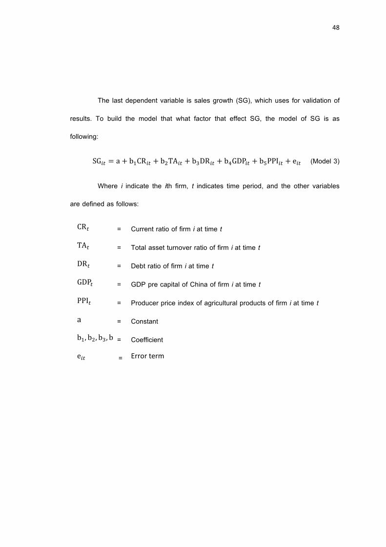
The last dependent variable is sales growth (SG), which uses for validation of

results. To build the model that what factor that effect SG, the model of SG is as

following:

SG!" = a+ b!CR!" + b!TA!" + b!DR!" + b!GDP!" + b!PPI!" + e!" (Model 3)

Where i indicate the ith firm, t indicates time period, and the other variables

are defined as follows:

CR! = Current ratio of firm i at time t

TA! = Total asset turnover ratio of firm i at time t

DR! = Debt ratio of firm i at time t

GDP! = GDP pre capital of China of firm i at time t

PPI! = Producer price index of agricultural products of firm i at time t

a = Constant

b!, b!, b!, b!, b! = Coefficient

e!"   =   Error  term  

50    

3.6 Hypothesis

Since the objective of this research is to examine the effects of liquidity,

asset utilization, leverage, economic prosperity and agricultural products price index

on financial performance of agricultural firms listed on Shanghai Stock Exchange.

The main hypotheses of this research are as follows:

Hypothesis1

Liquidity has positive effect on financial performance of agricultural firms listed on

Shanghai Stock Exchange.

Hypothesis 2

Asset utilization has positive effect on financial performance of agricultural firms listed

on Shanghai Stock Exchange.

Hypothesis 3

Leverage has negative effect on financial performance of agricultural firms listed on

Shanghai Stock Exchange.

Hypothesis 4

Economic prosperity has positive effect on financial performance of agricultural firms

listed on Shanghai Stock Exchange.

Hypothesis 5

Agricultural products price index has positive effect on financial performance of

agricultural firms listed on Shanghai Stock Exchange.  

CHAPTER 4

DATA ANALYSIS AND RESULTS

The purpose of this chapter is to discuss about the result of analysis from the

data collected based the conceptual framework. The following are topics in this chapter;

4.1 Unit – Root Test

4.2 Descriptive Statistics

4.3 Multicollinearity Test

4.4 Regression Results

52    

4.1 Unit – Root Test

To determine the factors affect financial performance of agricultural firms listed

on Shanghai Stock Exchange. The Unit Root Test is used to check the stationary

qualification before using the data because the non-stationary variables will influence the

behavior and properties of a series and result in a spurious regression. If the variable is

non-stationary, data should go for first differencing. If the stationary cannot be found at

the first difference, that may require further differencing. The results from Unit Root Test

show in Table 4.1.

Table 4.1 The results of Stationary Test by Unit – Root Test

Variables Levin, Lin & Chu Statistic Prob. Result

ROA -5.18680 0.0000 Stationary ROS -6.35813 0.0000 Stationary SG -3.65573 0.0001 Stationary CR -3.41916 0.0003 Stationary TA -3.83723 0.0001 Stationary DR -1.20070 0.1149 Non-Stationary

GDP 4.41278 1.0000 Non-Stationary PPI -6.60714 0.0000 Stationary

D(DR) -5.71823 0.0000 Stationary D(GDP) -6.16574 0.0000 Stationary

Table 4.1 shows results of Unit Root Test that the probability value of variable

ROA, ROS, SG, CR, TA and PPI is less than 0.05, it means variable ROA, ROS, SG,

CR, TA and PPI are stationary. But the probability value of variable DR and GDP is

greater than 0.05, it means variable DR and GDP are non-stationary. The first

53    

differencing should be applied to DR and GDP to make them stationary. After first

differencing DR and GDP, the probability value is less than 0.05. Therefore, variable

D(DR) and D(GDP) are stationary.

4.2 Descriptive Statistics

Table 4.2 Data Description

Variable Mean Median Max Min Std. Dev. Obs

ROA 0.007893 0.004821 1.181229 -0.812202 0.089283 299 ROS -0.175594 0.032327 86.27030 -50.25405 6.700780 299 SG 0.239895 0.045842 23.61445 -1.594806 1.715340 299 CR 1.402807 1.101501 11.12782 0.006377 1.297423 299 TA 0.145695 0.134497 1.135032 0.000973 0.095460 299

D(DR) -0.001070 -0.003690 2.876874 -3.539243 0.372660 299 D(GDP) 0.027950 0.548200 12.72300 -8.357000 4.318913 299

PPI 1.079265 1.073400 1.255400 0.933900 0.0927875 299

The above table summarized the data. Using descriptive statistics can show the

data more intuitive understanding of the data distribution. From the table 4.2 can know

the mean of each variable and Standard Deviation. This show that from 2006 to 2010,

variable ROA, ROS and SG denote the financial performance, average ROA is 0.008;

and its standard deviation is 0.089. The lowest ROA is -0.812 and the highest is 1.181.

For ROS, its mean is -0.176 and its standard deviation is 6.701. The minimum of ROS is

-50.254 and the maximum is 86.270. Finally, SG has its mean of 0.240 and standard

deviation of 1.715. The lowest SG is -1.595 and the highest is 23.614.

The independent variables include CR, TA, D(DR), D(GDP) and PPI. Variable

54    

CR denotes the liquidity, Mean of the CR is about 1.402 and its standard deviation is

1.297. The highest CR is around 11.128 and the lowest is 0.006. Variable TA denotes

the asset utilization. The average TA is 0.146 and the standard deviation is 0.095, the

highest value is 1.135 and the lowest value is 0.001. Variable DR denotes the leverage,

the D(DR) is the first differencing of DR. The maximum value of D(DR) is 2.877 and the

minimum value of D(DR) is -3.539, its mean is -0.001 and its standard deviation is

0.373. Variable GDP denotes the economic prosperity, and the D(GDP) is the first

differencing of GDP. The average quarterly D(GDP) of China is 0.028 trillion Yuan, the

highest value is 12.723 trillion Yuan and the lowest value is -8.357 trillion Yuan, the

standard deviation is 4.319 trillion Yuan. Variable PPI denotes the agricultural products

price index. Average quarterly PPI is1.079, the standard deviation is 0.093, the highest

value is 1.256 and the lowest value is 0.934. It means the inflation of agriculture

products is not large.

4.3 Multicollinearity Test

Test for multicollinearity will study the high pair – wise correlations and high

simple correlation coefficients because it can indicate the level of multicollinearity. If the

correlation between two explanatory variables is less than 0.80, there is no problem of

multicollinearity.

 

Table 4.3 The correlation of the independent variables

Correlation CR TA D(DR) D(GDP) PPI

CR 1.000000

55    

TA 0.269986 1.000000 D(DR) -0.014191 -0.070071 1.000000

D(GDP) -0.043438 0.150240 0.059831 1.000000 PPI -0.022966 0.016094 -0.025411 0.122203 1.000000

From the table 4.3, it shows the analysis for the correlations of independent

variables in the model. It is found that the value of correlation coefficient is not above

the limit value set for multicollinearity, which is less than 0.8. Therefore, there is no

multicollinearity problem. All the five independent variables can be used to run the

regressions.

 

4.4 Regression Results

In statistics, the Durbin – Watson statistic is a test statistic used to test the

existing of autocorrelation (a relationship between values separated from each other by

a given time lag) in the residuals (prediction errors) from a regression analysis. Durbin –

Watson statistics always lies between 0 and 4. When the value of Durbin – Watson

statistics must in the critical value range of Durbin – Watson statistics, there is no

autocorrelation problem. As this research have 299 observations and 5 independent

variables, checking the value from Durbin – Watson Statistics Value Table (Appendix F)

can get dL = 1.718 and dU = 1.820. The critical value range of Durbin – Watson

statistics is between 1.718 (dL) and 2.180 (4 – dU). The result of testing of Durbin –

Watson statistic must have the value between 1.718 and 2.180 in order to avoiding the

autocorrelation problem. The results from testing autocorrelation are as follows:

56    

4.4.1 Regression Results of Dependent Variable ROA

Table 4.4.1.1 Regression results of ROA

Variables C CR TA D(DR) D(GDP) PPI

Coefficient 0.011032 -0.002619 0.114815 -0.070023 0.0000985 -0.015076 Std. Error 0.058742 0.003968 0.054667 0.013323 0.001172 0.053597 t – Statistic 0.187812 -0.660008 2.100269 -5.255848 0.083982 -0.281280

Prob. 0.8512 0.5098 0.0366 0.0000 0.9331 0.7787

R – squared 0.104083 F – statistic 6.807846

Prob. 0.000005 Durbin –

Watson stat

2.223362

From the table 4.4.1.1, the regression equation of ROA can be written down as

following:

ROA = 0.011032 – 0.002619 CR + 0.114815 TA – 0.070023 D(DR) (0.187812) (-0.660008) (2.100269)* (-5.255848)**

57    

+ 0.0000985 D(GDP) – 0.015076 PPI (equation 1)

(0.083982) (-0.281280)

* = significant at the level of 0.05

** = significant at the level of 0.01

From the equation of ROA, it can see that the probability in the model equal to

0.000005 less than 0.01 at confidential level 99% that means all independence variables

in the model can use together for predicting dependence variable (ROA) at significant

statistic 0.01. 𝑅! equal to 0.104083 means that, the estimate equation can explain the

change of variables ROA by 10.4083%. The probability of TA equal to 0.0366 that

means TA is significant at 0.05 level. TA is a factor affecting the ROA. TA changes one

unit will make ROA changed by 0.114815 unit in the same direction. The probability of

D(DR) equal to 0.0000 that means D(DR) is significant at 0.01 level. D(DR) is a factor

affecting ROA. D(DR) changes one unit will make ROA changed by 0.070023 unit in the

opposite direction.

However, there is a problem of autocorrelation in the model of ROA. Because

the Durbin – Watson statistic of this model is 2.223362 greater than 2.180, therefore, it

needs to be addressed the autocorrelation of error function by ARMA process.

Table4.4.1.2 Adjusting regression results of ROA

Variables C CR TA D(DR) D(GDP) PPI

Coefficient 0.008786 -0.002526 0.113625 -0.080172 0.0000897 -0.013084 Std. Error 0.056985 0.004217 0.055348 0.014020 0.001390 0.051857

58    

t – Statistic 0.154182 -0.598918 2.052932 -5.718289 0.064517 -0.252307 Prob. 0.8776 0.5497 0.0410 0.0000 0.9486 0.8010

R – squared 0.114421 F – statistic 5.964960

Prob. 0.000007 Durbin –

Watson stat

2.142937

From the table 4.4.1.2, the adjusting regression equation of ROA after AR1

process can be written down as following:

ROA = 0.008786 – 0.002526 CR + 0.113625 TA – 0.080172 D(DR)

(0.154182) (-0.598918) (2.052932)* (-5.718289)**

+ 0.0000897 D(GDP) – 0.013084 PPI (equation 2)

(0.064517) (-0.252307)

* = significant at the level of 0.05

** = significant at the level of 0.01

From the equation of ROA, it can see that the probability in the model equal to

0.000007 less than 0.01 at confidential level 99% that means all independence variables

in the model can use together for predicting dependence variable (ROA) at significant

statistic 0.01. 𝑅!equal to 0.114421 means that, the estimate equation can explain the

change of variables ROA by 11.4421%. The probability of TA equal to 0.0410 that

means TA is significant at 0.05 level. TA is a factor that affects ROA. TA changes one

unit will make ROA changed by 0.113625 unit in the same direction The probability of

59    

D(DR) equal to 0.0000 that means D(DR) is significant at 0.01 level. D(DR) is a factor

that affects ROA; and the coefficient of D(DR)is negative number that means D(DR) is

inversely correlated with ROA. The changing of D(DR) affecting in the opposite direction

to the changing of financial performance of agricultural firms listed on Shanghai Stock

Exchange. D(DR) increases one unit will make ROA decreased by 0.080172 unit.

According to the results of Durbin – Watson statistic, it found that there is no

problem of autocorrelation in the model of ROA, because Durbin – Watson statistic is

2.142937 (between 1.718 and 2.180), means that, disturbance in the equation are

independently. So, this equation is the final equation of ROA.

4.4.2 Regression Results of Dependent Variable ROS

Table 4.4.2.1 Regression results of ROS

Variables C CR TA D(DR) D(GDP) PPI

Coefficient -2.245590 0.207601 3.874653 2.792499 -0.030047 1.128622 Std. Error 4.591056 0.310155 4.272581 1.041269 0.091635 4.188981 t – Statistic -0.489123 0.669345 0.906865 2.681821 -0.327902 0.269426

Prob. 0.6251 0.5038 0.3652 0.0077 0.7432 0.7878

R – squared 0.028409 F – statistic 1.713441

Prob. 0.131342 Durbin –

Watson stat

2.460880

From the table 4.4.2.1, the regression equation of ROS can be written down as

following:

60    

ROS = -2.245590 + 0.207601 CR + 3.874653 TA + 2.792499 D(DR)

(-0.489123) (0.669345) (0.906865) (2.681821)

- 0.030047 D(GDP) + 1.128622 PPI (equation 3)

(-0.327902) (0.269426)

From the equation of ROS, it shows that the probability in the model equal to

0.131342 that means no independent variables in this model affect ROS significantly.

Therefore, the model of ROS cannot be used to analyze the financial performance of

agricultural firms listed on Shanghai Stock Exchange.

4.4.3 Regression Results of Dependent Variable SG

Table 4.4.3.1 Regression results of SG

Variables C CR TA D(DR) D(GDP) PPI

Coefficient -2.580198 -0.108738 0.025476 -1.663562 0.006436 2.749055 Std. Error 1.091301 0.073724 1.015599 0.247511 0.021782 0.995728 t – Statistic -2.364331 -1.474924 0.025085 -6.721152 0.295460 2.760851

Prob. 0.0187 0.1413 0.9800 0.0000 0.7679 0.0061

R – squared 0.162282 F – statistic 11.35190

Prob. 0.000000 Durbin –

Watson stat

1.242603

61    

From the table 4.4.3.1, the regression equation of SG can be written down as

following:

SG = -2.580198 – 0.108738 CR + 0.025476 TA – 1.663562 D(DR)

(-2.364331) (-1.474924) (0.025085) (-6.721152)**

+ 0.006436 D(GDP) + 2.749055 PPI (equation 4)

(0.295460) (2.760851)**

* = significant at the level of 0.05

** = significant at the level of 0.01

From the equation of SG, it shows that the probability in the model equal to

0.000000 less than 0.01 at confidential level 99% that means all independence variables

in the model can use together for predicting dependence variable (SG) at significant

statistic 0.01. 𝑅! equal to 0.162282 means that, the estimate equation can explain the

change of variables SG by 16.2282%. The probability of D(DR) equal to 0.0000 that

means D(DR) is significant at 0.01 level. D(DR) is a factor affecting SG. D(DR) changes

one unit will make SG changed by 1.663562 unit in the opposite direction. The

probability of PPI equal to 0.0061 that means PPI is significant at 0.01 level. PPI is a

factor affecting SG; and the coefficient of PPI is positive number that means PPI is

positively correlation with SG. The changing of PPI affect in the same direction to the

changing of SG. PPI increases one unit will make SG increased by 2.749055 unit.

However, there is a problem of autocorrelation in the model of SG. Because

the Durbin – Watson statistic of this model is 1.242603 which is less than 1.718,

62    

therefore, it needs to be addressed the autocorrelation of error function by ARMA

process.

Table 4.4.3.2 Adjusting regression results of SG

Variables C CR TA D(DR) D(GDP) PPI

Coefficient -2.878397 -0.143041 1.197517 -1.135150 0.001815 2.896642 Std. Error 1.513365 0.124483 0.944156 0.282945 0.016574 1.370820 t – Statistic -1.901985 -1.149083 1.268347 -4.011913 0.109488 2.113072

Prob. 0.0582 0.2515 0.2057 0.0001 0.9129 0.0355

R – squared 0.318555 F – statistic 21.58149

Prob. 0.000000 Durbin –

Watson stat

1.765366

From the table 4.4.3.2, the regression equation of SG after AR1 process can

be written down as following:

SG = -2.878397 – 0.143041 CR + 1.197517 TA – 1.135150 D(DR)

(-1.901985) (-1.149083) (1.268347) (-4.011913)**

+ 0.001815 D(GDP) + 2.896642 PPI (equation 5)

(0.109488) (2.113072)*

* = significant at the level of 0.05

** = significant at the level of 0.01

63    

From the equation of SG, it shows that the probability in the model equal to

0.000000 less than 0.01 at confidential level 99% that means all independence variables

in the model can use together for predicting dependence variable (SG) at significant

statistic 0.01. 𝑅! equal to 0.318555 means that, the estimate equation can explain the

change of variables SG by 31.8555%. The probability of D(DR) equal to 0.0001 that

means D(DR) is significant at 0.01 level. D(DR) is factor affecting SG. D(DR) changes

one unit will make SG changed by 1.135150 unit in the opposite direction. The

probability of PPI equal to 0.0355 that means PPI is significant at 0.05 level. PPI is a

factor affecting SG. The changing of PPI affect in the positively direction to the changing

of the SG of agricultural firms litsed on Shanghai Stock Exchange. PPI increases one

unit will make SG changed by 2.896642 unit in the same direction.

According to the results of Durbin – Watson statistic, it found that there is no

problem of autocorrelation in the model of SG, because Durbin – Watson statistic is

1.765366 (between 1.718 and 2.180), means that, disturbance in the equation are

independently. So, this equation is the final equation of SG.

 

CHAPTER 5

CONCLUSION, DISCUSSION AND RECOMMENDATION

According to the results of analysis, this chapter will makes conclusion and

discussion about the factors affecting financial performance of agricultural firms listed on

Shanghai Stock Exchange and gives some suggestions.

5.1 Conclusion

5.2 Discussion

5.3 Implication of the Study

5.4 Research Recommendation

5.5 Limitations and Further Research

 

66    

5.1 Conclusion

This study examined the factors affecting financial performance of agricultural

firms listed on Shanghai Stock Exchange. This study is based on quarterly data of five

variables starting from January, 2006 to December 2010, totally 20 quarters. The data

includes financial information, economic information and agricultural industrial information

of a sample 15 companies over the period 2006 – 2010. Financial performance of firms

was measured by three financial indicators: return on assets, return on sales and sales

growth. Liquidity measured by current ratio. Asset utilization measured by total asset

turnover. Leverage measured by debt ratio. Economic prosperity measured by GDP.

Agricultural products price index measured by producer price index of agricultural

products.

In analyzing, some economic approaches were applied the data. First, testing

unit root of the original data found that debt ratio and GDP are non-stationary. Thus, the

first difference transformations of the original data was used; and then, testing the

correlation of each independent variable and autocorrelation among residuals by using

multiple regression with Ordinary Least Squares (OLS) Method.

Summarizing the results, this study considered just the variables that have

significantly statistic higher than 0.05 and the confidential level more than 95% to be the

factors that affecting to financial performance of agricultural firms listed on Shanghai

Stock Exchange. The results found that the variables that affecting to financial

performance of agricultural firms listed on Shanghai Stock Exchange are asset utilization

(total asset turnover ratio), leverage (debt ratio) and agricultural products price index,

67    

because they are statistically significant of the 0.05 level. Asset utilization and

agricultural products price index have positive correlation with firm financial performance,

but, leverage shows negative correlation with firm financial performance.

Furthermore, the results found that the liquidity and economic prosperity have

no effect on the changing of financial performance of agricultural firms listed on

Shanghai Stock Exchange.

Table 5.1 Summarize for testing hypothesis

Variable Hypothesis Conclusions Accept/Reject

Hypothesis

Liquidity Affect financial

performance Did not effect Reject

Asset Utilization Affect financial

performance Positively related Accept

Leverage Affect financial

performance Negatively related Accept

Economic Prosperity Affect financial

performance Did not effect Reject

Agricultural Products

Price Index

Affect financial

performance Positively related Accept

According to the table 5.1 which are summarized the study of the factors

affecting financial performance, in case of agricultural firms listed on Shanghai Stock

Exchange. It found that the asset utilization changing in the positive direction with

financial performance, the hypothesis is accepted; the leverage changing in the negative

68    

direction with financial performance, the hypothesis is accepted; agricultural products

price index changing in the positive direction with financial performance, the hypothesis

is accepted. The hypothesis of liquidity and economic prosperity are rejected in this

study, so they could not explain the change in financial performance of agricultural firms

listed on Shanghai Stock Exchange.

5.2 Discussion

5.2.1 Liquidity

The result of the study shows that the hypothesis of liquidity is rejected,

indicates that liquidity has no effect on financial performance of agricultural firms listed

on Shanghai Stock Exchange. This result is not consistent with the literature review.

However, empirical studies of Adams and Buckle (2003); Jose et al. (2010); Seema et

al. (2011); Sibel and Engin (2012) showed that there was a strong positive relationship

between liquidity and firms’ financial performance.

Liquidity is a ratio to measure a firm’s ability to payback short-term obligations.

The ability of payback short-term debt of agricultural firms listed on Shanghai Stock

Exchange is no effectively so as the ability to payback long-term debt. Therefore, it is

the reason why liquidity is not significant affecting on financial performance of

agricultural listed on Shanghai Stock Exchange.

69    

5.2.2 Asset Utilization

The result shows that asset utilization positively effects on financial

performance (ROA) of agricultural firms listed on Shanghai Stock Exchange. This result

was consistent with the findings of Jose et al. (2010); Wu, Li and Zhu (2010); Ding and

Sha (2011); Seema et al. (2011), the faster firm’s total asset turnover, the higher

efficiency of asset utilization and the better performance the firm has.

The positive correlation between asset utilization and financial performance

shows that the total asset turnover ratio is higher, the firm uses its assets more

productively and firm’s financial performance is better. As stated in Wu et al. (2010),

asset utilization made a great contribution to the profitability level of firm, and had a

significant positively effecting on the firm’s financial performance.

5.2.3 Leverage

In the ROA model, found that leverage has a negative correlation with financial

performance of agricultural firms listed on Shanghai Stock Exchange (coefficient equal to

-0.080172, probability less than 0.05); in the SG model, found that leverage has a

negative correlation with firms’ financial performance (coefficient equal to -1.663562,

probability less than 0.05). The negative result is in the line with the findings of Rajan

and Zingals (1995); Xiao (2005); Wu, Li and Zhu (2010).

China’s agricultural listed firms prefer long-term debt financing. The result found

that debt ratio is higher, the financial performance is worse. Because the firm has a high

70    

debt meaning the interest expense that the firm needs to pay is also high. The high

interest expense leads to low net income. Therefore, the firm’s financial performance will

get a negative effect from high debt. As stated in Mo (2008), a firm that has a capital

structure with a high debt will result in a bad firm performance.

5.2.4 Economic Prosperity

The result shows that the hypothesis of economic prosperity is rejected, so

economic prosperity has no effect on financial performance of agricultural firms listed on

Shanghai Stock Exchange. However, Deng et al. (2009) stated the higher rate of GDP

growth, the economic is boom and the level of profitability is high, then the firm

performance is better. Besides, Chen (2010), John and Riyas (2011) also got the same

result with Deng et al. (2009). Therefore, the result of this study is not consistent with

the literature review.

For China, gross domestic product (GDP) is the end results of the production

activities of all the resident units within China borders in a given period. This study used

the quarterly GDP, and the quarterly GDP has a growing trend. The average GDP

between 2006 and 2010 is 7.6929 trillion yuan. However, the production of agricultural

industry is a low percentage in GDP and has a decreasing trend year by year.

Therefore, GDP is not sufficient to explain the financial performance of agricultural listed

on Shanghai Stock Exchange.

71    

5.2.5 Agricultural Products Price Index

According the result of the model of SG shows that agricultural products price

index has effect on the financial performance of agricultural firms listed on Shanghai

Stock Exchange in the positive direction. This result was consistent with the literature

review. The early empirical studies demonstrated a positive relationship between

agricultural products price index and financial performance of agricultural firms listed on

Shanghai Stock Exchange (Demirguc-Kunt and Maksimovic, 1999; Booth et al., 2001;

Deng et al., 2009; Ma, 2011).

Andy (2001) pointed out that agricultural producer price index (PPI) is the

changes in prices that agricultural producer received from producing and selling the

agricultural commodities. So, PPI increase will lead to increase the revenue of

agricultural firms, and it will improve the firm performance.

5.3 Implication for the Study

This paper selected a number of factors to analyze correlation with financial

performance; and used multiple regressions to study factors affecting the financial

performance of agricultural firms listed on Shanghai Stock Exchange. From the empirical

research to explore the characteristics of the financial performance of agricultural firms

listed on Shanghai Stock Exchange.

According to the result of this study, showed that the financial performance of

agricultural firms listed on Shanghai Stock Exchange and the asset utilization have a

positive relationship. So, higher asset utilization will lead to high financial performance of

72    

agricultural firms. Asset utilization reflects the firm’s asset management. Total asset

turnover ratio reflects the operational ability of firms’ assets from the overall perspective.

The positive correlation showed that the assets operational ability is very important for

agricultural listed firms. It will directly affect the ability and speed of firm’s revenue

increasing and the scale expansion.

This study showed that the financial performance of agricultural firms listed on

Shanghai Stock Exchange and the leverage have a negative relationship. So, lower

leverage will bring high financial performance of agricultural firms. The negative relation

of financial performance and leverage could be expected on the fact that increases in

debt leads to increases in the firm’s financial and bankruptcy risk. It also reflected the

soft constraint condition in debt treatment of agricultural listed firms. In China, due to

many factors, the bankruptcy system exists in name only to lead to listed firms is unable

to establish risk awareness. Debt has no governance role in the decreasing financial

performance. The average debt ratio of agricultural firms listed on Shanghai Stock

Exchange is around 63.16%. It means the capital structure with high liabilities is not

suitable for the development of financial performance of agricultural firms listed on

Shanghai Stock Exchange. This passive liability increased the debt risk of firm and lead

to the development of long-term debt financing. Sample firms showed a trend that the

debt ratio is higher, the financial performance is worse. It reflected agricultural firms

listed on Shanghai Stock Exchange did not take advantage of the liabilities financing.

The financial leverage was not effectively used in agricultural firms listed on Shanghai

Stock Exchange.

73    

According to the result of this study, the financial performance of agricultural

firms listed on Shanghai Stock Exchange and the agricultural products price index have

a positive relationship. So, higher agricultural products price index will cause high

financial performance of agricultural firms. An increase in producer prices of finished

goods will results in consumer prices. This will cause an increase in firm income and

better the firm performance. Therefore, agricultural listed firms need to improve the

quality and added value of agricultural products to make sure the producer prices of

finished goods can increase within reasonable prices.

5.4 Research Recommendation

From the results of this study, asset utilization, leverage and agricultural

products price index are significant factors of financial performance of agricultural firms

listed on Shanghai Stock Exchange. Therefore, there are four recommendations as

following. The first recommendation is concluded by asset utilization; the second

recommendation and the third recommendation are concluded by leverage; and the

fourth recommendation is concluded by agricultural products price index.

First, Agricultural listed firms should develop targeted management plan based

on industry characteristics; improve the management level of agricultural listed firms;

build its brand image and create a good firm’s culture through learning advanced

management experience and combined with the firm features; strengthen the ability of

solvency and asset management of agricultural firms; speed up asset turnover to adapt

the firm’s development.

74    

Second, Agricultural listed firms should make full use of financial leverage and

tax shield to reduce the weighted average cost of capital; reasonable control long-term

debt ratio avoid the high financial risk and improve the financial performance of

agricultural firms listed on Shanghai Stock Exchange.

Third, Agricultural listed firms should improve the bankruptcy system to solve

the problem of the inefficient use of long-term debt financing and soft constraints of debt.

A sound firm bankruptcy system is precondition of the positively correlated between

leverage and firms financial performance. Establishing the security system of paying

debts and improving bank monitoring for agricultural listed firms in order to leverage has

a positive effect on agricultural listed firms.

Fourth, Agricultural listed firms should develop products to meet market

demand; improve the quality and added value of the agricultural products; Agricultural

listed firms should enhance the technological innovation capability and financial strength

of agricultural listed firms. Financial strength is the foundation of the creation and

operation of firms. Technological innovation is relied on by survival and development of

firms. Agricultural listed firms should establish cooperation relationship with scientific

research institutions to get the support in the development and promotion of new

varieties.

 

5.5 Limitations and Further Research

The limitations of this study are mainly reflected in:

75    

First, the sample size of agricultural listed firms is very small. According to

China Securities Regulatory Commission, there are 1718 listed firms in China but only

have 46 agricultural listed firms that accounted for only about 2.68% of the total number.

The data of this study collected financial statement of only 15 agricultural firms listed on

Shanghai Stock Exchange over 5 years, total 300 observations.

Second, this study used the quantitative research method and searched the

secondary data from listed firm’s website and National Bureau of Statistics. The data

may be not accurate, reliable, and authentic or has typing mistake to lead to the analysis

result is not accurate. So, the further research can be considered the quantitative

research method combined with qualitative research method and collected the primary

data by interviewing and surveying etc. to make sure the data is accurate.

Third, the result of this study showed that GDP is not significant for financial

performance of agricultural firms listed on Shanghai Stock Exchange. So, the further

research can be considered the gross agricultural production to be the independent

variable. And there are many factors affecting financial performance, it is difficult to

analysis each aspect. This study focused on liquidity, asset utilization, leverage,

economic prosperity and agricultural products price index, but didn’t analysis other

aspects.

In addition, the analysis idea of this study is very clear and the analysis method

is feasible. This study also can provide some contributions for the further research.

Further researches can consider the issues suggested by this study in other type of

firms or other factor of each aspect when analysis the factors affecting financial

76    

performance of listed firms. This study would add to the growing body of knowledge on

financial performance of listed firms.

77    

 

REFERENCES

Adams M. and Buckle M. (2003), “The Determinants of Corporate Financial

Performance in the Bermuda Insurance Market”, Applied Financial Economics

13: 133-143.

Altman, E. I. (1968), “Financial Ratios, Discriminant Analysis and the Prediction of

Corporate Bankruptcy”, Journal of Finance 23(4): 589-609.

Altman, E. I., Haldeman R. G. and Narayanan P. (1977), “ZETA Analysis: A New

Model to Identify Bankruptcy Risk of Corporations”, Journal of Banking & Finance

1(1): 29-54.

Ambrose, J. M. and Seward, J. A. (1988), “Best Rating Financial Ratios and Prior

Probabilities in Insolvency Prediction”, The Journal of Risk and Insurance 6: 229-

244.

Andy B. (2001), “The Redesign of the Canadian Farm Product Price Index”, Statistics

Canada 72(September): 3-19.

Athanasoglou, P. P, Brissimis, S. N. and Delis, M. D. (2008), “Bank-Specific, Industry-

Specific and Macroeconomic Determinants of Bank Profitability”, Journal of

International Financial Markets 18(2): 121-136.

Barry, P., Ellinger, P., Hopkin, J. and Baker, C. (1995), Financial Management in

Agriculture, Interstate Publishers, Danville, IL.

78    

 

Beaver, W. H. (1966), “Financial Ratios as Predictors of Failure”, Journal of Accounting

Research 4: 71-111.

Beaver, W. H. (1968), “Alternative Accounting Measures as Predictors of Failure,

Accounting Review 1: 113-122.

Bikker, J. A. and Hu, H., (2002) “Cyclical Patterns in Profits, Provisioning and Lending

of Banks and Procyclicality of the New Basel Capital Requirements”, BNL

Quarterly Review 221, pp. 143-175.

Branch (1983), “Serial Correlation and the Fixed Effects Model”, Review of Economic

Studies 49: 533-549.

Brilloff (1972), “An Examination of Commercial Bank Financial Ratios”, Journal of Bank

Research 9: 53-69.

Booth, L., V. Aivazian, A. Demirguc-Kunt, and V. Maksimovic (2001), “Capital

Structures in Developing Countries”, Journal of Finance 56: 87-130.

Bowen, H. (1978). Rationality. Legitimacy. Responsibility: Search for New Direction sin

Business and Society. Epstein. D. M. & Votaw. D. California: Goodyear

Publishing Company, Inc.

Chen, L. G. (2008), “An Empirical Analysis the Relationship between Capital Structure

and Firm Performance of the Listed Firms in SME Board“, Market Weekly 7: 83-

85.

79    

 

Chen, M. H. (2010), “The Economy, Tourism Growth and Corporate Performance in the

Taiwanese Hotel Industry”, Tourism Management 31: 665-675.

Chen Yu (2000), “An Empirical Study of Forecasting ST Firms Listed on China’s

Securities Market”, Economic Science 6: 57-67.

Claudio Giachetti (2012), “A Resource-based Perspective on the Relationship

BETWEEN Service Diversification and Firm Performance: Evidence from Italian

Facility Management Firms”, Journal of Business Economics and Management

13(3): 567-585.

Comett M. and Travlos H. (1989), “Institutional Ownership, Capital Structure, and Firm

Performance”, Strategic Management Journal, Vol. 12, pp. 479-491.

David, A. C., Frank, D. S., Betty J. S. and M. Gary, S. (2010), “The Gender and Ethnic

Diversity of US Boards and Board Committees and Firm Financial Performance”,

An International Review 18(5): 396-414.

Demirguc-Kunt, A. and V. Maksimovic. (1999), “Institutions, Financial Markets, and

Firm Debt Maturity”, Journal of Finance Economics 54: 295-336.

Deng Liguo and Luo Huawei (2009), “An Empirical Study of the Macroeconomic

Factors that Affect the Capital Structure of Agricultural Listed Companies”,

Journal of Market Modernization 11: 28-29.

80    

 

Ding Hua and Sha Rui (2011), “Empirical Analysis of the Impact of Capital Structure on

Performance in Jilin Forest Industry Co., Ltd”, Issues of Forestry Economics, Vol,

31 No. 2, pp. 141-144.

Engin Demirel, Ahmet Atakisi and Metin Atmaca (2011), “Financial and Economic

Factors Affecting Debt Ratio and ROE; ISE Tourism Firms Case”, European

Journal of Scientific Research, Vol. 61 No. 3, pp. 458-466.

Fazzari, E. F. and M. Jensen (1988), “Separation of Ownership and Control”, Journal

of Law and Economics, Vol. 26, No. 6, pp. 74-98.

Feng, G. F., Han, B. and Ruen, B. (2002), “An Empirical Research on Ownership

Concentration Changes of China’s Listed Companies”, Economic Research 8:

12-18.

Fu Hongzhen (2011), “Reviews of the Research on the Relationship between

Corporate Social Responsibility and Financial Performance”, Commercial

Research 412(August): 72-77.

Gao Yi (2010), Study on Formative Mechanism of Financial Risk and Control for

Agriculture Listed Companies in China, College of Economy and Management,

Southwest University, Beibei, Chongqing, China.

Gerwin Van der Laan, Hans Van Ees and Arjen Van Witteloostuijn (2007). “Corporate

Social and Financial Performance: An Extended Stakeholder Theory, and

81    

 

Empirical Test with Accounting Measures”, Journal of Business Ethics 79: 299-

310.

Gu Jibao and Guan Kai (2012), An Empirical Research on the Influential Factors of the

Listed Companies Performances in China, available at http://www.paper.edu.cn

(accessed May 17, 2012).

Guan Kai, Qiu Hao and Zhang Ying (2009), “An Analysis of External Factors Affecting

Firm Performance”, Journal of Statistics and Decision-Making 22: 181-183.

Hall, Hutchin and Charles W. L. (2000), “Diversified Growth and Competition: The

experience of twelve large UK firms”, Applied Economics, Vol. 17, No. 10,

pp.827-847.

Hao Xiangkun (2011), “An Analysis of Firms Performance Evaluation of Agricultural

Listed Firms Based on Factor Analysis”, Economic Research Guide 35: 124-125.

Hitt, M. A., Hoskisson, K. and Shimizu, K. (2006), “The Important of Resources in the

Internationalization of Professional Service Firms: the good, the bad and the

ugly”, Academy of Management Journal 49(6): 1137-1157.

Hong, X. X. and Shen, Y. F. (2002), “An Empirical Analysis of Factors Affecting Capital

Structure of China’s Listed Companies”, Journal if Xiamen University 3: 114-120.

Hu, R. and Michael A. (2006), “Antecedents and Performance Outcomes of

Diversification: A review and critique of theoretical perspectives”, Journal of

Management, Vol. 16, pp. 461-509.

82    

 

Israel (1989), Capital and Ownership Structure and the Market for Corporate Control

Working Paper, University of Michigan.

Jacqueline Murray Brux and Janna L. Cowen (1999), Econnomic Issues & Policy,

South-Western College Pulishing, OH, USA.

James C. Van Horne and John M. Wachowicz, JR. (2005), Fundamentals of Financial

Management, Prentice Hall: Financial Times, UK.

Jiang, Q. K. and Song, Y. H. (2005), “An Analysis of the Relationship between Debt

Structure and Business Performance of China’s Private Listed Companies “,

Technical Economic 5: 24-28.

John Manuel Luiz and Riyas Fadal (2011), “An Economic Analysis of Sports

Performance in Africa”, International Journal of Social Economics, Vol. 38 No.

10, pp. 869-883.

Jose Humberto Ablanedo-Rosas, Hongman Gao, Xiaochuan Zheng, Bahram Alidaee

and Haibo Wang (2010), “A Study of the Relative Efficiency of Chinese Ports: A

Financial Ratio-Based Data Envelopment Analysis Approach”, Expert Systems,

Vol. 27 No. 5, pp. 349-362.

Kakani, Ram Kumar and V. N. Reddy (1996), “Econometric Analysis of the Capital

Structure Determinants”, Decision, Vol. 23, Jan-Dec 1996, pp. 73-98.

Kim, B. Clark and Takahiro Fujimoto (1991), “Product Development Performance”,

Harvard Business School Press 1991.

83    

 

Kloptchenko. K. (1998), “Predicting Bankruptcies with the Self-organizing Map”,

Neurocomputing 21: 191-201.

Lam, M. (2004), “Neural Network Techniques for Financial Performance Prediction:

Integrating Fundamental and Technical Analysis”, Decision Support Systems

37(4): 567-581.

Lei Haizhang (2003), Modern Agricultural Economics, China Agriculture Press.

Li, G. Y. and Yang, L. (2010), “An Empirical Study of Capital Structure and Profitability

of SMEs—Based on Analysis Data of Small and Medium Enterprises Before and

After Listing on the SME Board”, Economic Review 1: 132-144.

Liu Qian (2010), “Establishing a Model of Firm Financial Performance Evaluation”,

Accounting and Auditing 6: 249-250.

Lu, J. W. and Beamish, P. W. (2004), “International Diversification and Firm

Performance: the S-curve Hypothesis”, Academy of Management Journal, Vol.

47 No. 4, pp. 598-609.

Lu, Z. F. and Xin, Y. (1998), “An Empirical Analysis of the Main Factors Affecting the

Capital Structure of Listed Companies”, Accounting Research 8: 97-98.

Ma Jinying (2011), “Empirical Research on Macroeconomic Factors Influences on

Capital Structure of Listed Agricultural Companies”, Journal of Economic

Geography, Vol. 31 No. 1, pp. 140-143.

84    

 

Mankiw S. H. (2007), “Financial Theory and Financial Strategy”, Interfaces, pp. 126-

137.

Maryanne M. Mowen and Don R. Hansen (2006), Management Accounting: The

Cornerstone for Business Decisions, Thomson South-Western, Ohio, USA.

Masulis and Ronald W. (1980), “The Effect of Capital Structure Change of Security: A

Study of Exchange Offers”, Journal of Financial Economics 8: 139-178.

McGuire, J. B., Sundgren, A. and Schneeweis, T. (1988), “Corporate Social

Responsibility and Firm Financial Performance”, Academy of Management

Journal, Vol. 31 No. 4, pp. 854-872.

McNamara, R. P., Cocks, N. and Hamilton, D. (1988), “Predicting Private Company

Failure”, Accounting and Finance, Vol. 28 No. 2, pp. 53-64.

Mo, S. (2008), “The Relationship between Growth, Profitability, and Firm Value”,

Strategic Management Journal, Vol. 8, pp. 487-497.

Moskowitz, M. (1975), “Profiles in Corporate Responsibility: The Ten Worst and the

Ten Best”, Business and Society Review 13: 28-42.

N. Gregory Mankiw (2007), Essentials of Economics, Thomson South-Western, OH,

USA.

85    

 

Olga Malikova and Zdenek Brabec (2012), “The Influence of a Different Accounting

System on Informative Value of Selected Financial Ratio”, Technological and

Economic Development of Economy 18(1): 149-163.

Ou, J. A. (1990), “The Information Content of Nonearning Accounting Numbers as

Earnings Predictors”, Journal of Accounting Research 28(1): 2-21.

Peng Yi (2006), “Study on the Operating Performance of the Agricultural Listed

Companies in China – Based on the Background of Transformation Economic”,

Zhengjiang University.

Peters, R., and Mullen, M. R., (2009), “Some Evidence of the Cumulative Effects of

Corporate Social Responsibility on Financial Performance”, Journal of Global

Business Issues 3: 1-14.

Qin, Z. G., Fu, L. M., Ma, C. and Li D. S. (2011), “Comparative Analysis of the

Development of Agricultural Listed Companies”, Journal of Anhui Agricultural

Science 39(10): 62-64.

Rajan, F. G. and Zingalas, L. (1995), “What Do We Know About Capital Structure –

Some Evidence from International Data”, Journal of Finance 50: 42-60.

Ram A. N. and Doran, H. (1996), “Testing for Granger Non-causality in Cointegrated

Systems Made Easy”, Working Paper in Econometrics and Applied Statistics No.

8, Department of Econometrics, University of New England, Armidale.

86    

 

Ram Kumar Kakani, Biswatosh Saha and V. N. Reddy (2003), “Determinants of

Financial Performance of Indian Corporate Sector in the Post-Liberalization Era:

An Exploratory Study”, NSE Research Initiative 5: 1- 38.

Ray McNamara and Keith Duncan (1995), Firm Performance and Macroeconomic

Variables, School of Business Discussion Papers, Paper 66.

Ruf, B. M., Muralidhar, K. and Paul, K. (1998), “The Development of a Systematic,

Aggregate Measure of Corporate Social Performance”, Journal of Management

24(1): 119-133.

Ruf, B. M., Muralidhar, K., Brown, R. M., Janey, J. J., and Paul, K. (2001), “An

Empirical Investigation of the Relathionship between Change in Corporate Social

Performance and Financial Performance: A Stakeholder Theory Perspective”,

Journal of Business Ethics 32(2): 143-156.

Schmalensee R. (1985), “Do Markets Differ Much?”, American Economic Review 75(3):

341-351.

Seema Gupta, P. K. Jain and Surendra S. Yadav (2011), “Impact of MoU on Financial

Performance of Public Sector Enterprises in India”, Journal of Advances in

Management Research, Vol. 8 No.2, pp. 263-284.

Selcuk Akcay (2011), “The Causal Relationship between Producer Price Index and

Consumer Price Index: Empirical Evidence from Selected European Countries”,

International Journal of Economics and Finance, Vol. 3 No. 6, pp. 227-232.

87    

 

Shi Qi (2009), An Empirical Study on the Impact on the Financial Performance of CSR

in China’s Listed Companies—Based on Real Estate Listed Companies,

Southwestern University of Finance and Economics.

Sibel Yilmaz Turkmen and Engin Demirel (2012), “Economic Factors Affecting Financial

Ratios; Real Estate Investment Trusts Case on ISE”, European Journal of

Scientific Research, Vol. 69 No. 1, pp. 42-51.

Stephen A. Ross, Randolph W. Westerfield and Bradford D. Jordan (2010),

Fundamentals of Corporate Finance, McGraw-Hill, New York, NY.

Steve Jackson, Roby Sawyers and Greg Jenkins (2006), Management Accounting,

Thomson South-Western, OH, USA.

Stigney (1990), “Financial Performance of Successful and Unsuccessful Farms”,

Journal of American Society of Farm Managers and Rural Appraisers, Vol. 54,

pp. 6-15.

Sun, J. (2011), “The Effect of Compensation Committee Quality on the Association

between CEO Cash Compensation and Accounting Performance”, Corporate

Governance: An International Review 17: 320-337.

Suwignjo, Bititci and Carrie (2000), “Quantitative Models for Performance Measurement

System”, International Journal of Production Economic 64: 231-241.

Titman S. and R. Wessels (1988), “The Determinants of Capital Structure Choice”,

Journal of Finance 53(1): 133-142.

88    

 

Vance, S. C. (1975), “Are Socially Responsible Corporations Good Investment Risks?”,

Academy of Management Review 64(8): 18-24.

Waddock, S. A., and Graves, S. B. (1997), “The Corporate Social Performance—

Financial Performance Link”, Strategic Management Journal 18(4): 303-319.

Wang Cuichun (2008), “Empirical Research on the Financial Evaluation of the Quality

of Listed Companies – Comment on the Financial Quality of the Listed

Agricultural Companies”, Shangdong Agricultural University.

Wang Juan and Yang Fenglin (2002), “An Analysis of the Factors Affecting Capital

Structure of China’s Listed Firms”, International Monetary Research 8: 45-52.

Wang Y. M. and Yang Y. (1998), “Fuzzy Data Envelopment Analysis Based upon

Fuzzy Arithmetic with an Application to Performance Assessment of

Manufacturing Enterprises”, Expert Systems with Application, Vol. 36, pp. 5205-

5211.

William J. Baumol and Alan S. Blinder (2001), “Economics Principles and Policy",

Harcourt College Publishers.

Wood, D. J. (1991), “Social Issues in Management: Theory and Research in Corporate

Social Performance”, Journal of Management 17(2): 383-406.

Wu Jing (2011), “Research of the Impact on China’s Economy by Fluctuations in

International Prices of Agricultural Products”, University of International Business

and Economics.

89    

 

Wu Jingxue, Li Yinan and Zhu Mei (2010), “Empirical Analysis of Rural Influencing

Factors on Listed Agribusiness Financial Performance”, Agricultural Economics

and Management 3: 22-27.

Wu shinong and Lu Xianyi (2001), “An Analysis of Forecasting Model of Financial

Distress Costs of China’s Listed Firms”, Economic Research 6: 46-55.

Wu Shinong and Zhang Zhiwang (2005), “An Analysis of Factors influencing Financial

Distress Costs of China’s Listed Firms”, Nankai Business Review 3: 101-106.

Xiao Zuoping (2005), “An Empirical Analysis of the Relationship between Capital

Structure and Firm Performance of Listed Firms”, Management Science 3: 16-22.

Yang Jingbo (2011), “An Empirical Study on Key Factors Affecting Performance of

China’s Listed Tourism Companies: Based on the Unbalanced Panel Data”,

Tourism Science, Vol. 25 No. 2, pp. 73-84.

Yao Dequan and Chen Xiaoxia (2008), “Research on Media Listed Firms’ Capital

Structure and Firm Performance”, Business Management 12: 71-75.

Yu Wei and Qian Yanmin (2009), “How the Macroeconomic Affects the Dynamic

Adjustment of Capital Structure in the Background of Transition Economies?”,

Proceedings of the Conference of National Doctoral Candidates: 1-15.

Zeng Saixing, Xie, X. M., Tam, C. M. and Wan, T. W. (2009), “Relationships between

Business Factors and Performance in Internationalization: An Empirical Study in

China”, Management Decision, Vol. 47 No. 2, pp: 308-329.

90    

 

Zhang Hangbo (2007), “Research and Application of Enterprise Financial Evaluation”,

Master’s Thesis of the School of Business Administration, Nanjing University of

Technology.

Zhang Xiangjian, Wang Xiaoming and Guo Lan (2010), “State-Owned Enterprises

Listing, Enterprise Performance and the Potential Factors”, Securities

Transactions Herald 8: 57-66.

Zhang Xiaoling (2010), “Based on Factor Analyzing: Performance Evaluation of Listed

Companies in SME Board and Its Factors Analysis”, Journal of Liuzhou Teachers

College, Vol. 25 No. 3, pp. 74-78.

Zhang Xicheng, Zhang Yanping and Zhang Jinhong (2006), “Stock Prediction Based

on Support Vector Machines”, Computer Technology and Development 6: 35-37.

Zhang, Z. G., He, W. F. and Liang, Z. G. (2007), “Capital Structure and Firm

Performance”, Journal of China Soft Science 12: 141-151.

Zhang Zhonghua (2010), “An Analysis of Executive Incentives Affecting on Financial

Performance”, Friends of Accounting 7: 29-31.

Zhu Daohua (2000), Agricultural Economics, China Agriculture Press.

 

   

APPENDICES

   

APPENDIX A

Unit – ROOT TEST

95    

 

1.1

Panel unit root test: Summary Series: ROA Date: 11/20/12 Time: 20:20 Sample: 2006Q1 2010Q4 Exogenous variables: Individual effects User-specified lags: 1 Newey-West automatic bandwidth selection and Bartlett kernel Balanced observations for each test Cross- Method Statistic Prob.** sections Obs

Null: Unit root (assumes common unit root process)

Levin, Lin & Chu t* -5.18680 0.0000 15 270

Null: Unit root (assumes individual unit root process)

Im, Pesaran and Shin W-stat -5.27873 0.0000 15 270 ADF - Fisher Chi-square 87.9884 0.0000 15 270 PP - Fisher Chi-square 119.758 0.0000 15 285 ** Probabilities for Fisher tests are computed using an asymptotic Chi -square distribution. All other tests assume asymptotic normality.

96    

 

1.2

Panel unit root test: Summary Series: ROS Date: 11/20/12 Time: 20:21 Sample: 2006Q1 2010Q4 Exogenous variables: Individual effects User-specified lags: 1 Newey-West automatic bandwidth selection and Bartlett kernel Balanced observations for each test Cross- Method Statistic Prob.** sections Obs

Null: Unit root (assumes common unit root process)

Levin, Lin & Chu t* -6.35813 0.0000 15 270

Null: Unit root (assumes individual unit root process)

Im, Pesaran and Shin W-stat -6.22439 0.0000 15 270 ADF - Fisher Chi-square 120.324 0.0000 15 270 PP - Fisher Chi-square 130.871 0.0000 15 285 ** Probabilities for Fisher tests are computed using an asymptotic Chi -square distribution. All other tests assume asymptotic normality.  

97    

 

1.3

Panel unit root test: Summary Series: SG Date: 11/20/12 Time: 20:21 Sample: 2006Q1 2010Q4 Exogenous variables: Individual effects User-specified lags: 1 Newey-West automatic bandwidth selection and Bartlett kernel Balanced observations for each test Cross- Method Statistic Prob.** sections Obs

Null: Unit root (assumes common unit root process)

Levin, Lin & Chu t* -3.65573 0.0001 15 270

Null: Unit root (assumes individual unit root process)

Im, Pesaran and Shin W-stat -3.86142 0.0001 15 270 ADF - Fisher Chi-square 64.1400 0.0003 15 270 PP - Fisher Chi-square 202.924 0.0000 15 285 ** Probabilities for Fisher tests are computed using an asymptotic Chi -square distribution. All other tests assume asymptotic normality.

98    

 

1.4

Panel unit root test: Summary Series: CR Date: 11/20/12 Time: 20:21 Sample: 2006Q1 2010Q4 Exogenous variables: Individual effects User-specified lags: 1 Newey-West automatic bandwidth selection and Bartlett kernel Balanced observations for each test Cross- Method Statistic Prob.** sections Obs

Null: Unit root (assumes common unit root process)

Levin, Lin & Chu t* -3.41916 0.0003 15 270

Null: Unit root (assumes individual unit root process)

Im, Pesaran and Shin W-stat -3.04955 0.0011 15 270 ADF - Fisher Chi-square 56.8648 0.0022 15 270 PP - Fisher Chi-square 79.2431 0.0000 15 285 ** Probabilities for Fisher tests are computed using an asymptotic Chi -square distribution. All other tests assume asymptotic normality.  

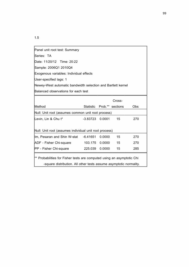
99    

 

1.5

Panel unit root test: Summary Series: TA Date: 11/20/12 Time: 20:22 Sample: 2006Q1 2010Q4 Exogenous variables: Individual effects User-specified lags: 1 Newey-West automatic bandwidth selection and Bartlett kernel Balanced observations for each test Cross- Method Statistic Prob.** sections Obs

Null: Unit root (assumes common unit root process)

Levin, Lin & Chu t* -3.83723 0.0001 15 270

Null: Unit root (assumes individual unit root process)

Im, Pesaran and Shin W-stat -6.41651 0.0000 15 270 ADF - Fisher Chi-square 103.175 0.0000 15 270 PP - Fisher Chi-square 225.039 0.0000 15 285 ** Probabilities for Fisher tests are computed using an asymptotic Chi -square distribution. All other tests assume asymptotic normality.

100    

 

1.6

Panel unit root test: Summary Series: DR Date: 11/20/12 Time: 20:22 Sample: 2006Q1 2010Q4 Exogenous variables: Individual effects User-specified lags: 1 Newey-West automatic bandwidth selection and Bartlett kernel Balanced observations for each test Cross- Method Statistic Prob.** sections Obs

Null: Unit root (assumes common unit root process)

Levin, Lin & Chu t* -1.20070 0.1149 15 270

Null: Unit root (assumes individual unit root process)

Im, Pesaran and Shin W-stat -1.45767 0.0725 15 270 ADF - Fisher Chi-square 42.3698 0.0665 15 270 PP - Fisher Chi-square 47.6173 0.0216 15 285 ** Probabilities for Fisher tests are computed using an asymptotic Chi -square distribution. All other tests assume asymptotic normality.    

101    

 

1.7

Panel unit root test: Summary Series: GDP Date: 11/20/12 Time: 20:22 Sample: 2006Q1 2010Q4 Exogenous variables: Individual effects User-specified lags: 1 Newey-West automatic bandwidth selection and Bartlett kernel Balanced observations for each test Cross- Method Statistic Prob.** sections Obs

Null: Unit root (assumes common unit root process)

Levin, Lin & Chu t* 4.41278 1.0000 15 270

Null: Unit root (assumes individual unit root process)

Im, Pesaran and Shin W-stat -0.18668 0.4260 15 270 ADF - Fisher Chi-square 21.8627 0.8590 15 270 PP - Fisher Chi-square 153.329 0.0000 15 285 ** Probabilities for Fisher tests are computed using an asymptotic Chi -square distribution. All other tests assume asymptotic normality.

102    

 

1.8

Panel unit root test: Summary Series: PPI Date: 11/20/12 Time: 20:23 Sample: 2006Q1 2010Q4 Exogenous variables: Individual effects User-specified lags: 1 Newey-West automatic bandwidth selection and Bartlett kernel Balanced observations for each test Cross- Method Statistic Prob.** sections Obs

Null: Unit root (assumes common unit root process)

Levin, Lin & Chu t* -6.60714 0.0000 15 270

Null: Unit root (assumes individual unit root process)

Im, Pesaran and Shin W-stat -6.67795 0.0000 15 270 ADF - Fisher Chi-square 98.6621 0.0000 15 270 PP - Fisher Chi-square 24.7855 0.7354 15 285 ** Probabilities for Fisher tests are computed using an asymptotic Chi -square distribution. All other tests assume asymptotic normality.  

   

103    

 

1.9

Panel unit root test: Summary Series: D(DR) Date: 11/20/12 Time: 20:39 Sample: 2006Q1 2010Q4 Exogenous variables: Individual effects User-specified lags: 1 Newey-West automatic bandwidth selection and Bartlett kernel Balanced observations for each test Cross- Method Statistic Prob.** sections Obs

Null: Unit root (assumes common unit root process)

Levin, Lin & Chu t* -5.71823 0.0000 15 255

Null: Unit root (assumes individual unit root process)

Im, Pesaran and Shin W-stat -8.03909 0.0000 15 255 ADF - Fisher Chi-square 122.743 0.0000 15 255 PP - Fisher Chi-square 246.128 0.0000 15 270 ** Probabilities for Fisher tests are computed using an asymptotic Chi -square distribution. All other tests assume asymptotic normality.

104    

 

1.10

Panel unit root test: Summary Series: D(GDP) Date: 11/20/12 Time: 20:39 Sample: 2006Q1 2010Q4 Exogenous variables: Individual effects User-specified lags: 1 Newey-West automatic bandwidth selection and Bartlett kernel Balanced observations for each test Cross- Method Statistic Prob.** sections Obs

Null: Unit root (assumes common unit root process)

Levin, Lin & Chu t* -6.16574 0.0000 15 255

Null: Unit root (assumes individual unit root process)

Im, Pesaran and Shin W-stat -13.6487 0.0000 15 255 ADF - Fisher Chi-square 202.815 0.0000 15 255 PP - Fisher Chi-square 3950.86 0.0000 15 270 ** Probabilities for Fisher tests are computed using an asymptotic Chi -square distribution. All other tests assume asymptotic normality.  

APPENDIX B

DESCRIPTIVE STATISTICS

 

106    

 

ROA ROS SG CR TA DDR DGDP PPI

Mean 0.007893 -0.175594 0.239895 1.402807 0.145695 -0.001070 0.027950 1.079265 Median 0.004821 0.032327 0.045842 1.101501 0.134497 -0.003690 0.548200 1.073400 Maximum 1.181229 86.27030 23.61445 11.12782 1.135032 2.876874 12.72300 1.255400 Minimum -0.812202 -50.25405 -1.594806 0.006377 0.000973 -3.539243 -8.357000 0.933900 Std. Dev. 0.089283 6.700780 1.715340 1.297423 0.095460 0.372660 4.318913 0.092875 Skewness 5.173573 4.685434 11.16411 4.854595 4.103429 -0.621374 0.521272 0.292239 Kurtosis 125.2142 109.4114 140.7256 30.51791 40.50428 50.26009 5.219198 2.096723 Jarque-Bera 187415.2 142164.5 242525.1 10608.32 18362.63 27845.13 74.89628 14.42081 Probability 0.000000 0.000000 0.000000 0.000000 0.000000 0.000000 0.000000 0.000739 Sum 2.360048 -52.50265 71.72874 419.4393 43.56281 -0.319965 8.357000 322.7003 Sum Sq. Dev. 2.375480 13380.33 876.8325 501.6252 2.715532 41.38495 5558.597 2.570506 Observations 299 299 299 299 299 299 299 299

 

APPENDIX C MULTICOLLINEARITY TEST

   

108    

 

ROA ROS SG CR TA DDR DGDP PPI

ROA 1.000000 0.509779 0.045907 -0.000617 0.133425 -0.299649 0.005456 -0.004824 ROS 0.509779 1.000000 0.031415 0.053377 0.052511 0.149309 -0.001616 0.009295 SG 0.045907 0.031415 1.000000 -0.080856 0.009367 -0.363156 0.016555 0.161921 CR -0.000617 0.053377 -0.080856 1.000000 0.269986 -0.014191 -0.043438 -0.022966 TA 0.133425 0.052511 0.009367 0.269986 1.000000 -0.070071 0.150240 0.016094

DDR -0.299649 0.149309 -0.363156 -0.014191 -0.070071 1.000000 0.059831 -0.025411 DGDP 0.005456 -0.001616 0.016555 -0.043438 0.150240 0.059831 1.000000 0.122203 PPI -0.004824 0.009295 0.161921 -0.022966 0.016094 -0.025411 0.122203 1.000000

 

APPENDIX D REGRESSION

 

110    

 

2.1

Dependent Variable: ROA Method: Panel Least Squares Date: 11/20/12 Time: 20:28 Sample: 2006Q1 2010Q4 Periods included: 20 Cross-sections included: 15 Total panel (unbalanced) observations: 299

Variable Coefficient Std. Error t-Statistic Prob. C 0.011032 0.058742 0.187812 0.8512

CR -0.002619 0.003968 -0.660008 0.5098 TA 0.114815 0.054667 2.100269 0.0366

DDR -0.070023 0.013323 -5.255848 0.0000 DGDP 9.85E-05 0.001172 0.083982 0.9331 PPI -0.015076 0.053597 -0.281280 0.7787

R-squared 0.104083 Mean dependent var 0.007893

Adjusted R-squared 0.088794 S.D. dependent var 0.089283 S.E. of regression 0.085227 Akaike info criterion -2.067141 Sum squared resid 2.128233 Schwarz criterion -1.992884 Log likelihood 315.0375 Hannan-Quinn criter. -2.037420 F-statistic 6.807846 Durbin-Watson stat 2.223362 Prob(F-statistic) 0.000005

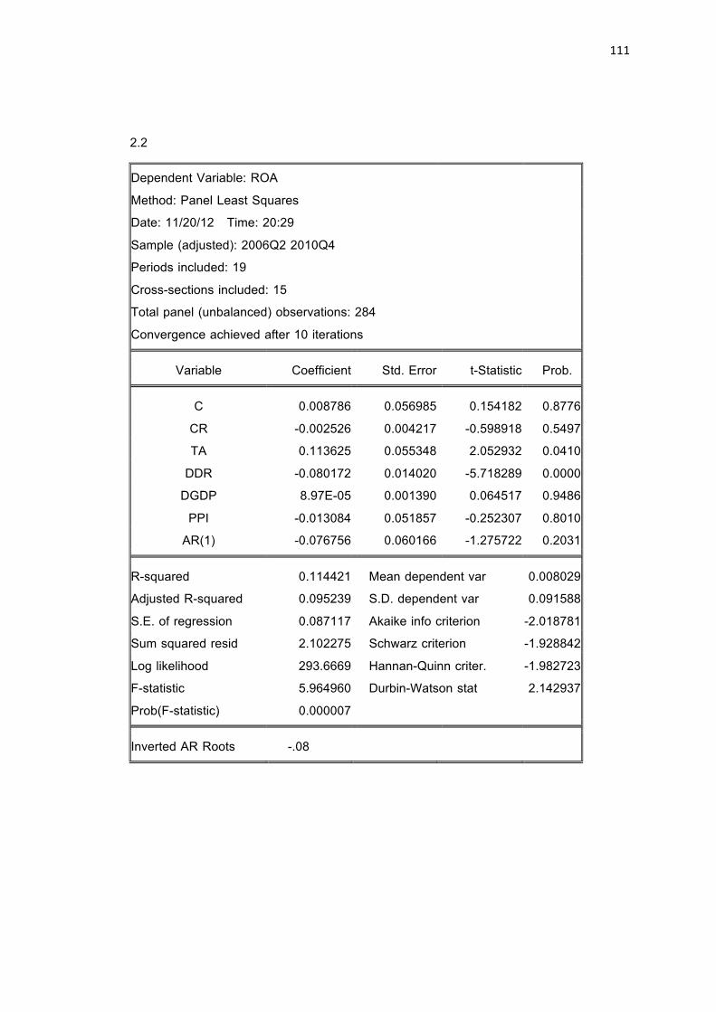
111    

 

2.2

Dependent Variable: ROA Method: Panel Least Squares Date: 11/20/12 Time: 20:29 Sample (adjusted): 2006Q2 2010Q4 Periods included: 19 Cross-sections included: 15 Total panel (unbalanced) observations: 284 Convergence achieved after 10 iterations

Variable Coefficient Std. Error t-Statistic Prob. C 0.008786 0.056985 0.154182 0.8776

CR -0.002526 0.004217 -0.598918 0.5497 TA 0.113625 0.055348 2.052932 0.0410

DDR -0.080172 0.014020 -5.718289 0.0000 DGDP 8.97E-05 0.001390 0.064517 0.9486 PPI -0.013084 0.051857 -0.252307 0.8010

AR(1) -0.076756 0.060166 -1.275722 0.2031 R-squared 0.114421 Mean dependent var 0.008029

Adjusted R-squared 0.095239 S.D. dependent var 0.091588 S.E. of regression 0.087117 Akaike info criterion -2.018781 Sum squared resid 2.102275 Schwarz criterion -1.928842 Log likelihood 293.6669 Hannan-Quinn criter. -1.982723 F-statistic 5.964960 Durbin-Watson stat 2.142937 Prob(F-statistic) 0.000007

Inverted AR Roots -.08

112    

 

2.3

Dependent Variable: ROS Method: Panel Least Squares Date: 11/20/12 Time: 20:30 Sample: 2006Q1 2010Q4 Periods included: 20 Cross-sections included: 15 Total panel (unbalanced) observations: 299

Variable Coefficient Std. Error t-Statistic Prob. C -2.245590 4.591056 -0.489123 0.6251

CR 0.207601 0.310155 0.669345 0.5038 TA 3.874653 4.272581 0.906865 0.3652

DDR 2.792499 1.041269 2.681821 0.0077 DGDP -0.030047 0.091635 -0.327902 0.7432 PPI 1.128622 4.188981 0.269426 0.7878

R-squared 0.028409 Mean dependent var -0.175594

Adjusted R-squared 0.011829 S.D. dependent var 6.700780 S.E. of regression 6.661030 Akaike info criterion 6.650288 Sum squared resid 13000.21 Schwarz criterion 6.724545 Log likelihood -988.2181 Hannan-Quinn criter. 6.680009 F-statistic 1.713441 Durbin-Watson stat 2.460880 Prob(F-statistic) 0.131342

113    

 

2.4

Dependent Variable: SG Method: Panel Least Squares Date: 11/20/12 Time: 20:30 Sample: 2006Q1 2010Q4 Periods included: 20 Cross-sections included: 15 Total panel (unbalanced) observations: 299

Variable Coefficient Std. Error t-Statistic Prob. C -2.580198 1.091301 -2.364331 0.0187

CR -0.108738 0.073724 -1.474924 0.1413 TA 0.025476 1.015599 0.025085 0.9800

DDR -1.663562 0.247511 -6.721152 0.0000 DGDP 0.006436 0.021782 0.295460 0.7679 PPI 2.749055 0.995728 2.760851 0.0061

R-squared 0.162282 Mean dependent var 0.239895

Adjusted R-squared 0.147986 S.D. dependent var 1.715340 S.E. of regression 1.583338 Akaike info criterion 3.776810 Sum squared resid 734.5388 Schwarz criterion 3.851066 Log likelihood -558.6331 Hannan-Quinn criter. 3.806531 F-statistic 11.35190 Durbin-Watson stat 1.242603 Prob(F-statistic) 0.000000

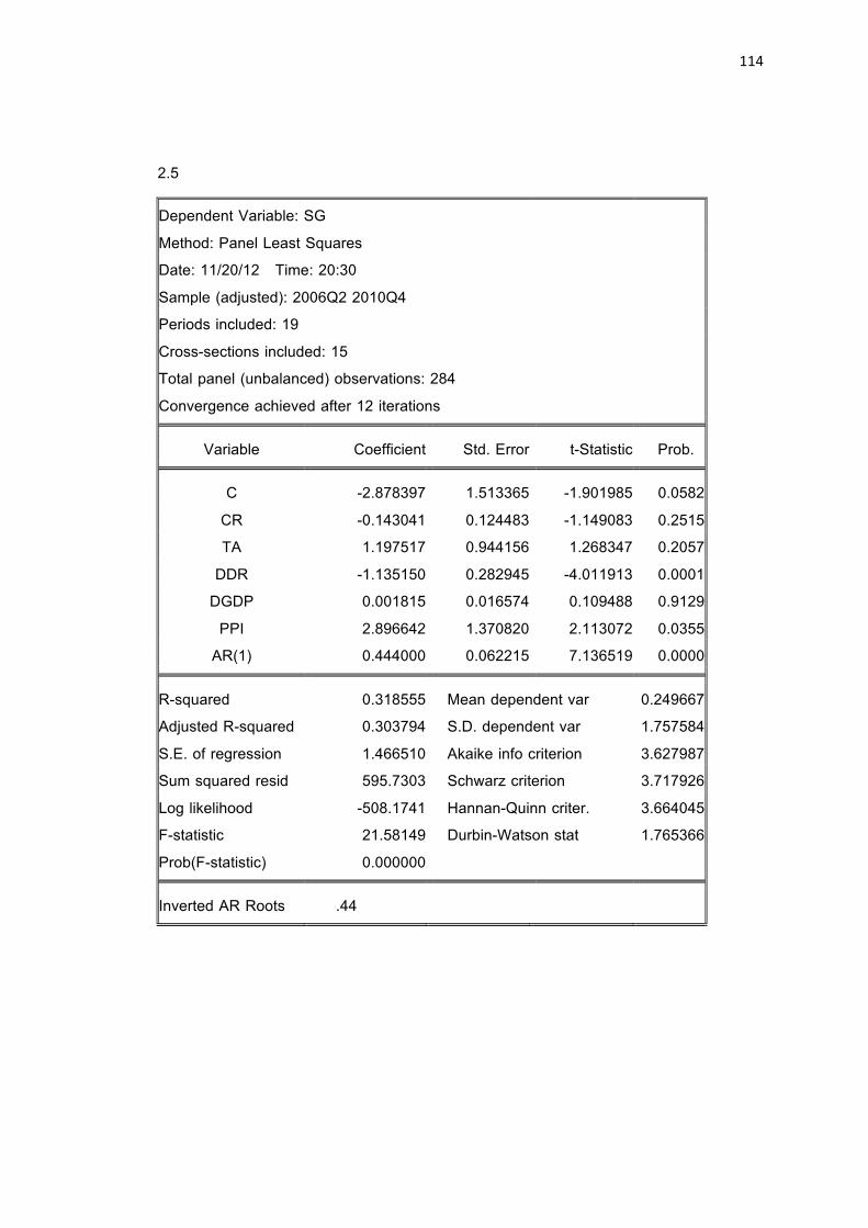
114    

 

2.5

Dependent Variable: SG Method: Panel Least Squares Date: 11/20/12 Time: 20:30 Sample (adjusted): 2006Q2 2010Q4 Periods included: 19 Cross-sections included: 15 Total panel (unbalanced) observations: 284 Convergence achieved after 12 iterations

Variable Coefficient Std. Error t-Statistic Prob. C -2.878397 1.513365 -1.901985 0.0582

CR -0.143041 0.124483 -1.149083 0.2515 TA 1.197517 0.944156 1.268347 0.2057

DDR -1.135150 0.282945 -4.011913 0.0001 DGDP 0.001815 0.016574 0.109488 0.9129 PPI 2.896642 1.370820 2.113072 0.0355

AR(1) 0.444000 0.062215 7.136519 0.0000 R-squared 0.318555 Mean dependent var 0.249667

Adjusted R-squared 0.303794 S.D. dependent var 1.757584 S.E. of regression 1.466510 Akaike info criterion 3.627987 Sum squared resid 595.7303 Schwarz criterion 3.717926 Log likelihood -508.1741 Hannan-Quinn criter. 3.664045 F-statistic 21.58149 Durbin-Watson stat 1.765366 Prob(F-statistic) 0.000000

Inverted AR Roots .44  

APPENDIX E

DURBIN – WATSON STATISTICS VALUE TABLE

 

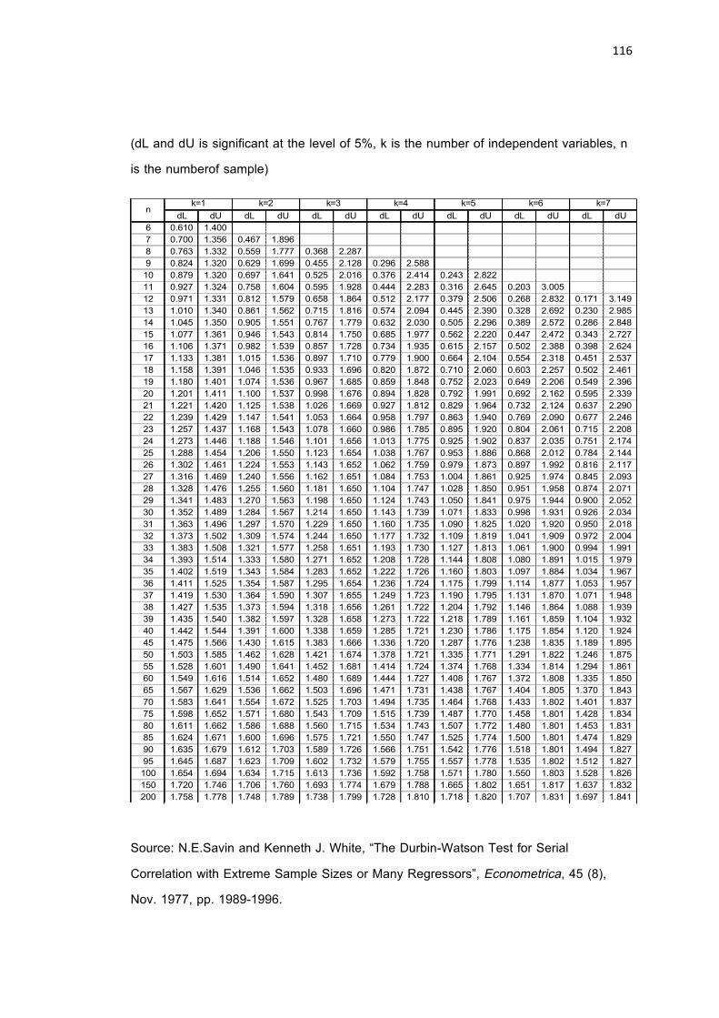
116    

 

(dL and dU is significant at the level of 5%, k is the number of independent variables, n

is the numberof sample)

Source: N.E.Savin and Kenneth J. White, “The Durbin-Watson Test for Serial

Correlation with Extreme Sample Sizes or Many Regressors”, Econometrica, 45 (8),

Nov. 1977, pp. 1989-1996.

dL dU dL dU dL dU dL dU dL dU dL dU dL dU6 0.610 1.4007 0.700 1.356 0.467 1.8968 0.763 1.332 0.559 1.777 0.368 2.2879 0.824 1.320 0.629 1.699 0.455 2.128 0.296 2.58810 0.879 1.320 0.697 1.641 0.525 2.016 0.376 2.414 0.243 2.82211 0.927 1.324 0.758 1.604 0.595 1.928 0.444 2.283 0.316 2.645 0.203 3.00512 0.971 1.331 0.812 1.579 0.658 1.864 0.512 2.177 0.379 2.506 0.268 2.832 0.171 3.14913 1.010 1.340 0.861 1.562 0.715 1.816 0.574 2.094 0.445 2.390 0.328 2.692 0.230 2.98514 1.045 1.350 0.905 1.551 0.767 1.779 0.632 2.030 0.505 2.296 0.389 2.572 0.286 2.84815 1.077 1.361 0.946 1.543 0.814 1.750 0.685 1.977 0.562 2.220 0.447 2.472 0.343 2.72716 1.106 1.371 0.982 1.539 0.857 1.728 0.734 1.935 0.615 2.157 0.502 2.388 0.398 2.62417 1.133 1.381 1.015 1.536 0.897 1.710 0.779 1.900 0.664 2.104 0.554 2.318 0.451 2.53718 1.158 1.391 1.046 1.535 0.933 1.696 0.820 1.872 0.710 2.060 0.603 2.257 0.502 2.46119 1.180 1.401 1.074 1.536 0.967 1.685 0.859 1.848 0.752 2.023 0.649 2.206 0.549 2.39620 1.201 1.411 1.100 1.537 0.998 1.676 0.894 1.828 0.792 1.991 0.692 2.162 0.595 2.33921 1.221 1.420 1.125 1.538 1.026 1.669 0.927 1.812 0.829 1.964 0.732 2.124 0.637 2.29022 1.239 1.429 1.147 1.541 1.053 1.664 0.958 1.797 0.863 1.940 0.769 2.090 0.677 2.24623 1.257 1.437 1.168 1.543 1.078 1.660 0.986 1.785 0.895 1.920 0.804 2.061 0.715 2.20824 1.273 1.446 1.188 1.546 1.101 1.656 1.013 1.775 0.925 1.902 0.837 2.035 0.751 2.17425 1.288 1.454 1.206 1.550 1.123 1.654 1.038 1.767 0.953 1.886 0.868 2.012 0.784 2.14426 1.302 1.461 1.224 1.553 1.143 1.652 1.062 1.759 0.979 1.873 0.897 1.992 0.816 2.11727 1.316 1.469 1.240 1.556 1.162 1.651 1.084 1.753 1.004 1.861 0.925 1.974 0.845 2.09328 1.328 1.476 1.255 1.560 1.181 1.650 1.104 1.747 1.028 1.850 0.951 1.958 0.874 2.07129 1.341 1.483 1.270 1.563 1.198 1.650 1.124 1.743 1.050 1.841 0.975 1.944 0.900 2.05230 1.352 1.489 1.284 1.567 1.214 1.650 1.143 1.739 1.071 1.833 0.998 1.931 0.926 2.03431 1.363 1.496 1.297 1.570 1.229 1.650 1.160 1.735 1.090 1.825 1.020 1.920 0.950 2.01832 1.373 1.502 1.309 1.574 1.244 1.650 1.177 1.732 1.109 1.819 1.041 1.909 0.972 2.00433 1.383 1.508 1.321 1.577 1.258 1.651 1.193 1.730 1.127 1.813 1.061 1.900 0.994 1.99134 1.393 1.514 1.333 1.580 1.271 1.652 1.208 1.728 1.144 1.808 1.080 1.891 1.015 1.97935 1.402 1.519 1.343 1.584 1.283 1.652 1.222 1.726 1.160 1.803 1.097 1.884 1.034 1.96736 1.411 1.525 1.354 1.587 1.295 1.654 1.236 1.724 1.175 1.799 1.114 1.877 1.053 1.95737 1.419 1.530 1.364 1.590 1.307 1.655 1.249 1.723 1.190 1.795 1.131 1.870 1.071 1.94838 1.427 1.535 1.373 1.594 1.318 1.656 1.261 1.722 1.204 1.792 1.146 1.864 1.088 1.93939 1.435 1.540 1.382 1.597 1.328 1.658 1.273 1.722 1.218 1.789 1.161 1.859 1.104 1.93240 1.442 1.544 1.391 1.600 1.338 1.659 1.285 1.721 1.230 1.786 1.175 1.854 1.120 1.92445 1.475 1.566 1.430 1.615 1.383 1.666 1.336 1.720 1.287 1.776 1.238 1.835 1.189 1.89550 1.503 1.585 1.462 1.628 1.421 1.674 1.378 1.721 1.335 1.771 1.291 1.822 1.246 1.87555 1.528 1.601 1.490 1.641 1.452 1.681 1.414 1.724 1.374 1.768 1.334 1.814 1.294 1.86160 1.549 1.616 1.514 1.652 1.480 1.689 1.444 1.727 1.408 1.767 1.372 1.808 1.335 1.85065 1.567 1.629 1.536 1.662 1.503 1.696 1.471 1.731 1.438 1.767 1.404 1.805 1.370 1.84370 1.583 1.641 1.554 1.672 1.525 1.703 1.494 1.735 1.464 1.768 1.433 1.802 1.401 1.83775 1.598 1.652 1.571 1.680 1.543 1.709 1.515 1.739 1.487 1.770 1.458 1.801 1.428 1.83480 1.611 1.662 1.586 1.688 1.560 1.715 1.534 1.743 1.507 1.772 1.480 1.801 1.453 1.83185 1.624 1.671 1.600 1.696 1.575 1.721 1.550 1.747 1.525 1.774 1.500 1.801 1.474 1.82990 1.635 1.679 1.612 1.703 1.589 1.726 1.566 1.751 1.542 1.776 1.518 1.801 1.494 1.82795 1.645 1.687 1.623 1.709 1.602 1.732 1.579 1.755 1.557 1.778 1.535 1.802 1.512 1.827100 1.654 1.694 1.634 1.715 1.613 1.736 1.592 1.758 1.571 1.780 1.550 1.803 1.528 1.826150 1.720 1.746 1.706 1.760 1.693 1.774 1.679 1.788 1.665 1.802 1.651 1.817 1.637 1.832200 1.758 1.778 1.748 1.789 1.738 1.799 1.728 1.810 1.718 1.820 1.707 1.831 1.697 1.841

k=1 k=2 k=3 k=4 k=5 k=6 k=7n

117  

BIOGRAPHY

Ms. Wei Wei was born on 09 July 1988. She received a Bachelor Degree in

International Business and trade from the GUANGXI UNIVERSITY FOR NATIONALITY

in year 2010.