Factorial ANOVA: More than one categorical explanatory

variable

STA312 Fall 2012

See last slide for copyright information

Factorial ANOVA •  Categorical explanatory variables are called

factors •  More than one at a time •  Originally for true experiments, but also useful

with observational data

•  If there are observations at all combinations of explanatory variable values, it’s called a complete factorial design (as opposed to a fractional factorial).

The potato study

•  Cases are storage containers (of potatoes) •  Same number of potatoes in each container.

Inoculate with bacteria, store for a fixed time period.

•  Response variable is number of rotten potatoes.

•  Two explanatory variables, randomly assigned –  Bacteria Type (1, 2, 3) –  Temperature (1=Cool, 2=Warm)

Two-factor design

Bacteria Type Temp 1 2 3

1=Cool

2=Warm

Six treatment conditions

Factorial experiments •  Allow more than one factor to be

investigated in the same study: Efficiency!

•  Allow the scientist to see whether the effect of an explanatory variable depends on the value of another explanatory variable: Interactions

•  Thank you again, Mr. Fisher.

Normal with equal variance and conditional (cell) means

Bacteria Type Temp 1 2 3

1=Cool

2=Warm

Tests

•  Main effects: Differences among marginal means

•  Interactions: Differences between differences (What is the effect of Factor A? It depends on Factor B.)

To understand the interaction, plot the means

Temperature by Bacteria Interaction

0

5

10

15

20

25

1 2 3

Bacteria Type

Ro

t Cool

Warm

Either Way

Temperature by Bacteria Interaction

0

5

10

15

20

25

1 2 3

Bacteria Type

Ro

t Cool

Warm

Temperature by Bacteria Interaction

0

5

10

15

20

25

Cool Warm

TemperatureR

ot

Bact 1

Bact 2

Bact 3

Non-parallel profiles = Interaction

It Depends

0

5

10

15

20

25

1 2 3

Bacteria Type

Mean

Ro

t

Cool

Warm

Main effects for both variables, no interaction

Main Effects Only

0

5

10

15

20

25

1 2 3

Bacteria Type

Mean

Ro

t

Cool

Warm

Main effect for Bacteria only

0

5

10

15

20

25

30

35

Cool Warm

Temperature

Mean

Ro

t

Bact 1

Bact 2

Bact 3

Main Effect for Temperature Only

Temperature Only

0

5

10

15

20

25

1 2 3

Bacteria Type

Mean

Ro

t

Cool

Warm

Both Main Effects, and the Interaction

Mean Rot as a Function of Temperature

and Bacteria Type

0

5

10

15

20

25

1 2 3

Bacteria Type

Ro

t Cool

Warm

Should you interpret the main effects?

It Depends

0

5

10

15

20

25

1 2 3

Bacteria Type

Mean

Ro

t

Cool

Warm

Testing for Interactions

• 

• 

Main Effects Only

0

5

10

15

20

25

1 2 3

Bacteria Type

Mean

Ro

tCool

Warm

Equivalent statements

•  The effect of A depends upon B •  The effect of B depends on A

Three factors: A, B and C

•  There are three (sets of) main effects: One each for A, B, C

•  There are three two-factor interactions –  A by B (Averaging over C) –  A by C (Averaging over B) –  B by C (Averaging over A)

•  There is one three-factor interaction: AxBxC

Meaning of the 3-factor interaction

•  The form of the A x B interaction depends on the value of C

•  The form of the A x C interaction depends on the value of B

•  The form of the B x C interaction depends on the value of A

•  These statements are equivalent. Use the one that is easiest to understand.

To graph a three-factor interaction

•  Make a separate mean plot (showing a 2-factor interaction) for each value of the third variable.

•  In the potato study, a graph for each type of potato

Four-factor design

•  Four sets of main effects •  Six two-factor interactions •  Four three-factor interactions •  One four-factor interaction: The nature

of the three-factor interaction depends on the value of the 4th factor

•  There is an F test for each one •  And so on …

As the number of factors increases

•  The higher-way interactions get harder and harder to understand

•  All the tests are still tests of differences between differences of differences …

•  But it gets complicated •  Effect coding to the rescue

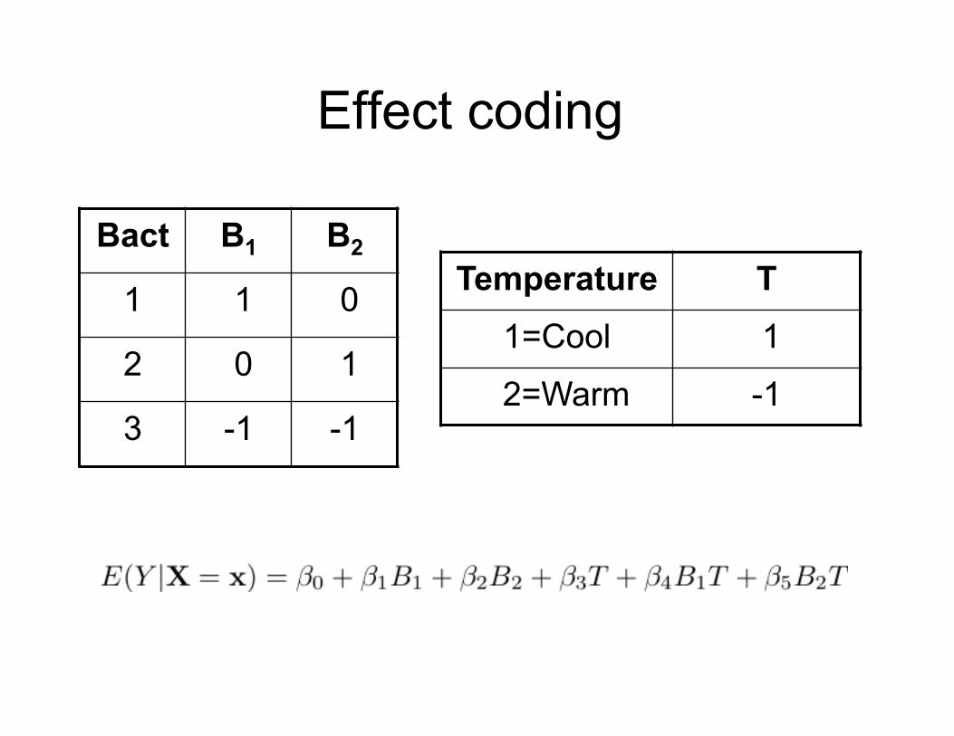
Effect coding

Bact B1 B2

1 1 0

2 0 1

3 -1 -1

Temperature T 1=Cool 1

2=Warm -1

Interaction effects are products of dummy variables

•  The A x B interaction: Multiply each dummy variable for A by each dummy variable for B

•  Use these products as additional explanatory variables in the multiple regression

•  The A x B x C interaction: Multiply each dummy variable for C by each product term from the A x B interaction

•  Test the sets of product terms simultaneously

Make a table

Bact Temp B1 B2 T B1T B2T

1 1 1 0 1 1 0

1 2 1 0 -1 -1 0

2 1 0 1 1 0 1

2 2 0 1 -1 0 -1

3 1 -1 -1 1 -1 -1

3 2 -1 -1 -1 1 1

Cell and Marginal Means

Bacteria Type Tmp 1 2 3

1=C

2=W

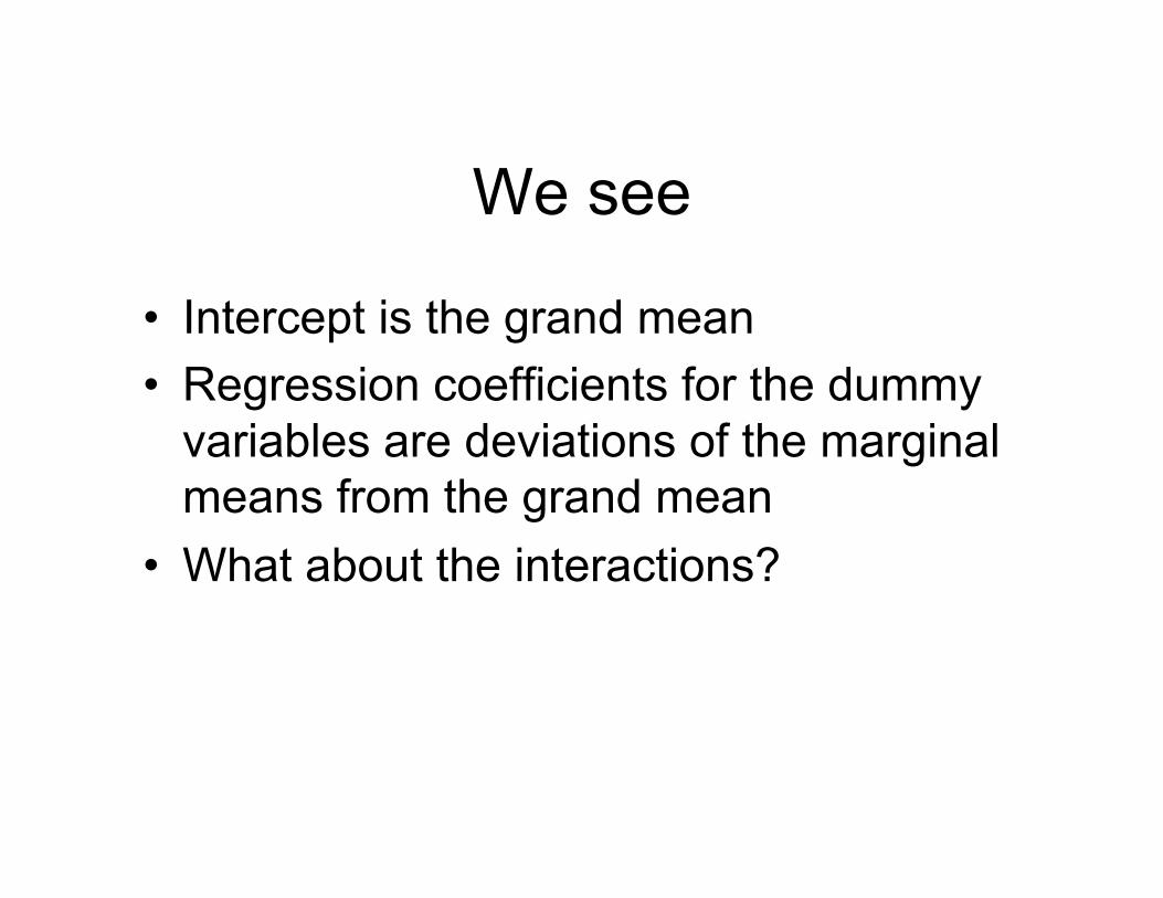
We see

•  Intercept is the grand mean •  Regression coefficients for the dummy

variables are deviations of the marginal means from the grand mean

•  What about the interactions?

A bit of algebra shows

What are “effects?”

•  There are 3 main effects for Bacteria Type: beta1, beta2 and -beta1 -beta2.

•  They are deviations of the marginal means from the grand mean. •  There are 2 main effects for Temperature: beta3 and - beta3 •  They are deviations of the marginal means from the grand mean. •  There are 6 interaction effects. •  They are deviations of the cell mean from the grand mean plus the

main effects. •  They add to zero across rows and across columns. •  The non-redundant ones are beta4 and beta5.

•  This is regression notation. There are ANOVA notations as well.

Factorial ANOVA with effect coding is pretty automatic

•  You don’t have to make a table unless asked •  It always works as you expect it will •  Significance tests are the same as testing

sets of contrasts •  Covariates present no problem. Main effects

and interactions have their usual meanings, “controlling” for the covariates.

•  Could plot the least squares means

Again

•  Intercept is the grand mean •  Regression coefficients for the dummy

variables are deviations of the marginal means from the grand mean

•  Test of main effect(s) is test of the dummy variables for a factor.

•  Interaction effects are products of dummy variables.

Balanced vs. Unbalanced Experimental Designs

•  Balanced design: Cell sample sizes are proportional (maybe equal)

•  Explanatory variables have zero relationship to one another

•  Numerator SS in ANOVA are independent •  Everything is nice and simple •  Most experimental studies are designed this

way. •  As soon as somebody drops a test tube, it’s

no longer true

Analysis of unbalanced data •  When explanatory variables are related, there

is potential ambiguity. •  A is related to Y, B is related to Y, and A is

related to B. •  Who gets credit for the portion of variation in

Y that could be explained by either A or B? •  With a regression approach, whether you use

contrasts or dummy variables (equivalent), the answer is nobody.

•  Think of full, reduced models. •  Equivalently, general linear test

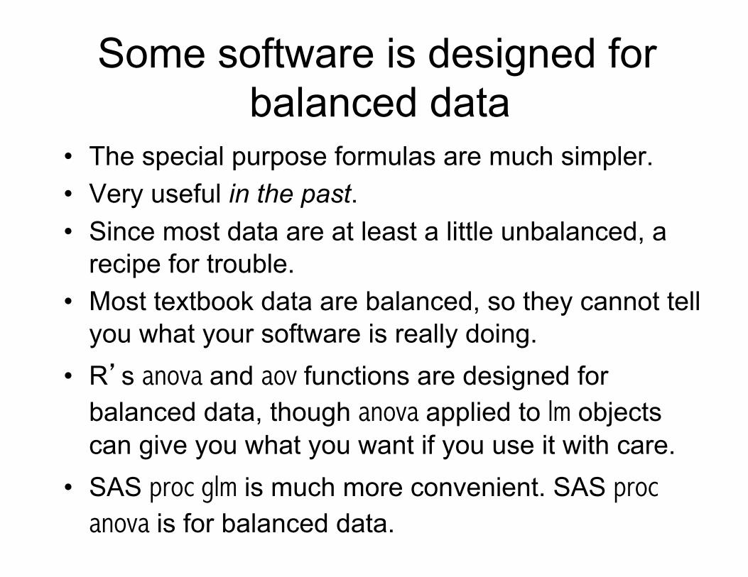
Some software is designed for balanced data

•  The special purpose formulas are much simpler. •  Very useful in the past. •  Since most data are at least a little unbalanced, a

recipe for trouble. •  Most textbook data are balanced, so they cannot tell

you what your software is really doing. •  R’s anova and aov functions are designed for

balanced data, though anova applied to lm objects can give you what you want if you use it with care.

•  SAS proc glm is much more convenient. SAS proc anova is for balanced data.

Rotten potatoes with R

> spuds = read.table("http://www.utstat.toronto.edu/~brunner/312f12

/code_n_data/potato2.data")

> attach(spuds)

> bact = factor(Bact); temp = factor(Temp)

> # Table of means

> meanz = tapply(Rot,INDEX=list(temp,bact),FUN=mean); meanz

1 2 3

1 3.555556 4.777778 8.00000

2 7.000000 13.555556 19.55556

> # Make it prettier

> Labels = NULL # Make an empty list for row, col labels

> Labels$Temp = c("Low","High")

> Labels$Bacteria = c("1","2","3")

> dimnames(meanz) = Labels

> # Could use rownames, colnames instead

> meanz = addmargins(meanz,FUN=mean) # Add marginal means

> meanz = round(meanz,2) # Round to 2 decimal places

> meanz

Bacteria

Temp 1 2 3 mean

Low 3.56 4.78 8.00 5.44

High 7.00 13.56 19.56 13.37

mean 5.28 9.17 13.78 9.41

Two-factor ANOVA > # Two-factor ANOVA

> table(temp,bact)

bact

temp 1 2 3

1 9 9 9

2 9 9 9

> # Balanced design. aov is safe

> summary(aov(Rot ~ temp + bact + temp:bact))

Df Sum Sq Mean Sq F value Pr(>F)

temp 1 848.1 848.1 38.614 1.18e-07 ***

bact 2 651.8 325.9 14.839 9.61e-06 ***

temp:bact 2 152.9 76.5 3.481 0.0387 *

Residuals 48 1054.2 22.0

---

Signif. codes: 0 ‘***’ 0.001 ‘**’ 0.01 ‘*’ 0.05 ‘.’ 0.1 ‘ ’ 1

# Get same results with Rot ~ temp*bact

One more comment about the potatoes

Note that aov is smart enough to produce the right tests even with indicator dummy variables. If you wanted to reproduce the tests for main effects with regression you'd use effect coding.

More about Interactions •  Interaction between independent

variables means “It depends.” •  Relationship between one explanatory

variable and the response variable depends on the value of another explanatory variable.

•  Can have – Quantitative by quantitative – Quantitative by categorical – Categorical by categorical

Quantitative by Quantitative

Y = �0 + �1x1 + �2x2 + �3x1x2 + ⇥

E(Y |x) = �0 + �1x1 + �2x2 + �3x1x2

For fixed x2

E(Y |x) = (�0 + �2x2) + (�1 + �3x2)x1

Both slope and intercept depend on value of x2

And for fixed x1, slope and intercept relating x2 to E(Y) depend on the value of x1

Quantitative by Categorical

•  Interaction means slopes are not equal •  Form a product of quantitative variable by

each dummy variable for the categorical variable

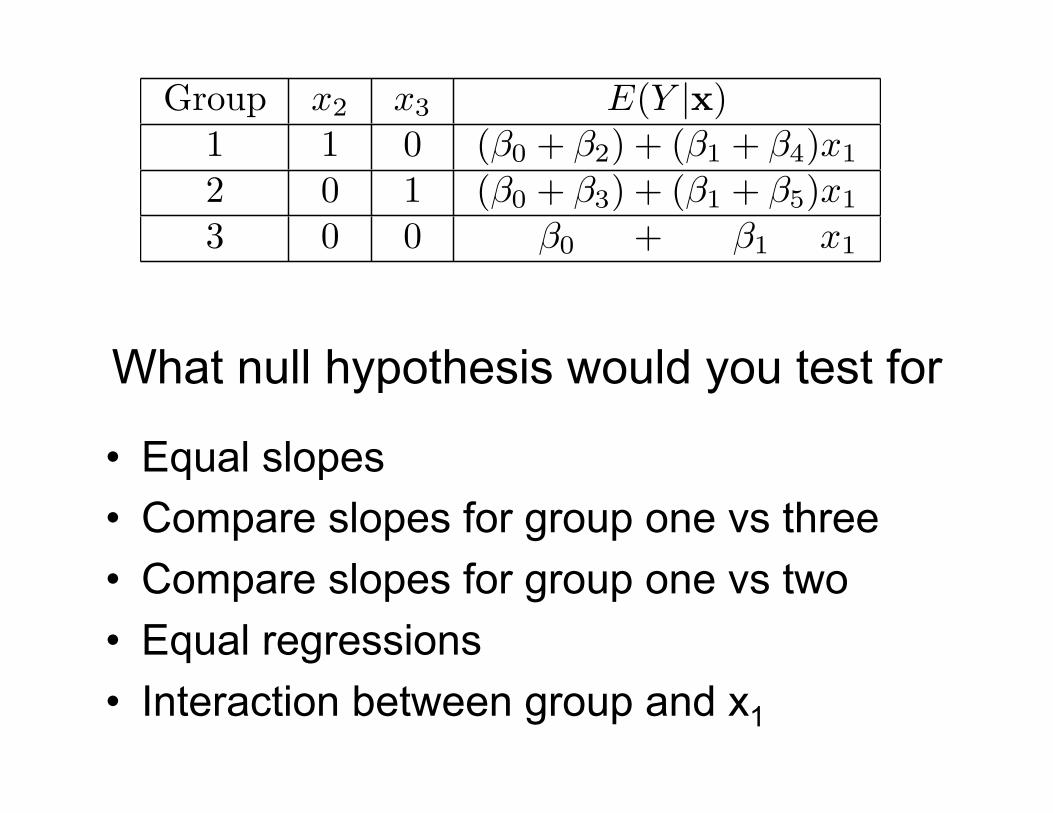
•  For example, three treatments and one covariate: x1 is the covariate and x2, x3 are dummy variables

Y = �0 + �1x1 + �2x2 + �3x3

+�4x1x2 + �5x1x3 + ⇥

E(Y |x) = �0 + �1x1 + �2x2 + �3x3 + �4x1x2 + �5x1x3

Group x2 x3 E(Y |x)1 1 0 (�0 + �2) + (�1 + �4)x1

2 0 1 (�0 + �3) + (�1 + �5)x1

3 0 0 �0 + �1 x1

Group x2 x3 E(Y |x)1 1 0 (�0 + �2) + (�1 + �4)x1

2 0 1 (�0 + �3) + (�1 + �5)x1

3 0 0 �0 + �1 x1

What null hypothesis would you test for

•  Equal slopes •  Compare slopes for group one vs three •  Compare slopes for group one vs two •  Equal regressions •  Interaction between group and x1

What to do if H0: β4=β5=0 is rejected

•  How do you test Group “controlling” for x1? •  A good choice is to set x1 to its sample mean,

and compare treatments at that point.

•  How about setting x1 to sample mean of the group (3 different values)?

•  With random assignment to Group, all three means just estimate E(X1), and the mean of all the x1 values is a better estimate.

Copyright Information

This slide show was prepared by Jerry Brunner, Department of Statistics, University of Toronto. It is licensed under a Creative Commons Attribution - ShareAlike 3.0 Unported License. Use any part of it as you like and share the result freely. These Powerpoint slides will be available from the course website: http://www.utstat.toronto.edu/brunner/oldclass/312f12 The potato data set is from Minitab, and is used here without permission.