FACILITATING NO-NOTICE EVACUATION … NO-NOTICE EVACUATION THROUGH OPTIMAL PICK-UP LOCATION...

FACILITATING NO-NOTICE EVACUATION THROUGH OPTIMAL PICK-UP LOCATION SELECTION

FINAL REPORT

DTRS99-G-0003

Prepared for

Mid-Atlantic University Transportation Center

By

Sirui Liu, Graduate Research Assistant Dr. Pamela Murray-Tuite, Principal Investigator

Department of Civil and Environment Engineering Northern Virginia Center

Virginia Polytechnic Institute and State University 7054 Haycock Road, Falls Church, VA 22043

August 2009

1

1. Report No.

2. Government Accession No. 3. Recipient’s Catalog No.

4. Title and Subtitle Facilitating No-Notice Evacuation through Optimal Pick-up Location Selection

5. Report Date August 2009 6. Performing Organization Code VT-2007-01

7. Author(s) Sirui Liu and Pamela Murray-Tuite, Ph.D.

8. Performing Organization Report No.

9. Performing Organization Name and Address Virginia Polytechnic Institute and State University, Blacksburg Virginia Tech Transportation Institute 3500 Transportation Research Plaza Blacksburg, Virginia 24061

10. Work Unit No. (TRAIS) 11. Contract or Grant No. DTRS99-G-0003

12. Sponsoring Agency Name and Address Virginia Transportation Research Council 530 Edgemont Road Charlottesville, VA 22903

13. Type of Report and Period Covered Final Report 1/1/2008 – 8/9/2008 14. Sponsoring Agency Code

15. Supplementary Notes 16. Abstract Under no-notice disasters, dependents in facilities such as schools and daycare centers usually wait for their families to pick them up. This family pickup behavior could increase individual evacuation time and cause extra delay to other vehicles in the network. Relocating the dependents to other pickup sites may facilitate no-notice evacuation. This study developed an optimization model to determine optimal pickup locations, assuming that all evacuating families have personal vehicles; the objective is to maximize the number of evacuees who can successfully pick up dependents and then escape from the dangerous zones within a safe evacuation time threshold. The optimization model was based on anticipated travel time output from the simulation model (VISSIM in this study); iteration between the two models was performed. The methodology was applied to a case study based on a simplified version of Chicago Heights, Illinois. The case study involved three facilities with 492 dependents and three safe time thresholds (i.e., 30, 45 and 60 minutes). Improvements in total travel time, average speed, total delay time and average delay time per vehicle and increases in the number of successful evacuations of dependents were used to evaluate the performance of the relocation strategy. This study also examined the sensitivity of the strategy to parents’ arrival time, number of dependents, and safe time. Finally, relocation sites were recommended based on the results of all scenarios. The results found that the relocation strategy was sensitive to safe evacuation time and number of pickup evacuees (pickup evacuees refer to those persons with a need to pick up their dependents inside the dangerous zones). The relocation strategy was prominently effective when safe evacuation time fell into a moderate range or the number of pickup evacuees was fairly high. Application of the proposed methodology to a certain area can assist local decision-makers to take effective measures during no-notice evacuation and the relocation sites could be part of local evacuation management plans. 17. Key Words Evacuation, no-notice, household gathering

18. Distribution Statement No restrictions. This document is available to the public.

19. Security Classif. (of this report) Unclassified

20. Security Classif. (of this page) Unclassified

21. No. of Pages 42

22. Price N/A

2

Abstract

Under no-notice disasters, dependents in facilities such as schools and daycare centers usually wait for their families to pick them up. This family pickup behavior could increase individual evacuation time and cause extra delay to other vehicles in the network. Relocating the dependents to other pickup sites may facilitate no-notice evacuation. This study developed an optimization model to determine optimal pickup locations, assuming that all evacuating families have personal vehicles; the objective is to maximize the number of evacuees who can successfully pick up dependents and then escape from the dangerous zones within a safe evacuation time threshold. The optimization model was based on anticipated travel time output from the simulation model (VISSIM in this study); iteration between the two models was performed. The methodology was applied to a case study based on a simplified version of Chicago Heights, Illinois. The case study involved three facilities with 492 dependents and three safe time thresholds (i.e., 30, 45 and 60 minutes). Improvements in total travel time, average speed, total delay time and average delay time per vehicle and increases in the number of successful evacuations of dependents were used to evaluate the performance of the relocation strategy. This study also examined the sensitivity of the strategy to parents’ arrival time, number of dependents, and safe time. Finally, relocation sites were recommended based on the results of all scenarios. The results found that the relocation strategy was sensitive to safe evacuation time and number of pickup evacuees (pickup evacuees refer to those persons with a need to pick up their dependents inside the dangerous zones). The relocation strategy was prominently effective when safe evacuation time fell into a moderate range or the number of pickup evacuees was fairly high. Application of the proposed methodology to a certain area can assist local decision-makers to take effective measures during no-notice evacuation and the relocation sites could be part of local evacuation management plans.

3

Table of Contents

Abstract ......................................................................................................................................................................... 2 Table of Contents........................................................................................................................................................... 3 List of Figures ................................................................................................................................................................ 4 List of Tables ................................................................................................................................................................. 5 Chapter 1 Introduction ......................................................................................................................................... 6 Chapter 2 Literature Review ................................................................................................................................ 8

2.1 Regional Evacuation .................................................................................................................................... 8 2.1.1. Aggregate Evacuation Modeling ......................................................................................................... 8 2.1.2. Disaggregate Evacuation Modeling ..................................................................................................... 9

2.2 Neighborhood Evacuation ............................................................................................................................ 9 2.3 No-notice Evacuation ................................................................................................................................. 10 2.4 Shelter Location ......................................................................................................................................... 10 2.5 Facility Location Problem .......................................................................................................................... 10

Chapter 3 Methodology ..................................................................................................................................... 12 3.1 Optimization Model ................................................................................................................................... 12 3.2 Traffic Simulation Model ........................................................................................................................... 15 3.3 Framework ................................................................................................................................................. 15 3.4 Pickup Trip Generation .............................................................................................................................. 18

Chapter 4 Case Study ......................................................................................................................................... 19 4.1 Network Description .................................................................................................................................. 19 4.2 Selecting Relocation Sites .......................................................................................................................... 20 4.3 Evacuation Demand Estimation ................................................................................................................. 22

4.3.1 Non-pickup Evacuee Estimation ....................................................................................................... 22 4.3.2 Pickup Evacuee Estimation ............................................................................................................... 22

4.4 Other Assumptions and Modeling Considerations ..................................................................................... 23 4.5 Result Analysis .......................................................................................................................................... 23

4.5.1 Improvements of MOEs .................................................................................................................... 24 4.5.2 SP indicators ....................................................................................................................................... 26

4.6 Sensitivity Analysis .................................................................................................................................... 28 4.6.1 Sensitivity to pickup evacuee arrival time distribution ( , ) and T0 ............................................. 28

4.6.2 Sensitivity to total number of pickup evacuees ................................................................................. 32 4.7 Recommended sets of relocation sites ........................................................................................................ 34

Chapter 5 Summary and Conclusions ................................................................................................................ 38 References ................................................................................................................................................................... 40

4

List of Figures

Figure 1 Flowchart of the Study .................................................................................................................................. 16 Figure 2 Overview of the Actual Network (http://www.maps.google.com) ................................................................ 19 Figure 3 Overview of the Modeled Network in VISSIM ............................................................................................ 20 Figure 4 Locations of Facilities and Relocation Sites .................................................................................................. 21 Figure 5 Average Speed (mph) for Each Iterated Run ................................................................................................. 26 Figure 6 SP Indicators over Iterated Runs .................................................................................................................... 27 Figure 7 Pickup Evacuees Arrival Time Distribution Scenarios ................................................................................. 28

5

List of Tables

Table 1 Comparison between Short-notice Evacuation and No-notice Evacuation ...................................................... 6 Table 2 Walking Distance (in Miles) among Facilities/Sites....................................................................................... 21 Table 3 Indicators of whether Main Streets Must Be Crossed to Move Children from a Given Facility to a Given Site

....................................................................................................................................................................... 21 Table 4 Comparisons of MOEs with and without Relocation Strategy Implemented ................................................. 25 Table 5 Improvements of MOEs with the Relocation Strategy implemented (T0=30minutes) ................................... 29 Table 6 Improvements of MOEs with the Relocation Strategy implemented (T0=45minutes) ................................... 29 Table 7 Improvements of MOEs with the Relocation Strategy implemented (T0=60minutes) ................................... 30 Table 8 Optimal Sets of Relocation Sites under Different Demand Scenarios ............................................................ 31 Table 9 Comparisons of Improvements of MOEs between Original Demand and Increased Demand (20, 2.5) ........ 32 Table 10 Comparisons of Improvements of MOEs between Original Demand and Increased Demand (20, 5) ......... 33 Table 11 Comparisons of Optimal Sets of Relocation Sites between Original Demand and Increased Demand ........ 34 Table 12 Comparisons of Improvements of MOEs between Determined Optimal Relocation Set and Recommend

Set (T0=30minutes) ..................................................................................................................................... 35 Table 13 Comparisons of Improvements of MOEs between Determined Optimal Relocation Set and Recommend

Set (T0=45minutes) ..................................................................................................................................... 36 Table 14 Comparisons of Improvements of MOEs between Determined Optimal Relocation Set and Recommend

Set (T0=60minutes) ..................................................................................................................................... 37

6

Chapter 1 Introduction

A huge disaster usually requires an efficient evacuation. Based on the disaster’s characteristics, an evacuation can be classified into short-notice and no-notice. A short-notice evacuation is usually associated with a disaster event that is relatively predicable, i.e., forecasting the occurrence of the event is feasible (Chiu et al, 2007). A hurricane is an example of an event causing a “short-notice evacuation”. Conversely, no-notice evacuation is associated with unpredictable disasters, such as nuclear explosions, terrorist attacks and hazardous materials (hazmat) releases. An evacuation that starts immediately after the occurrence of a disaster event is defined as a “no-notice evacuation” (Pearce, 2008). The terrorist attack of September 11, 2001, causing nearly 3000 fatalities and destroying the 110-story Twin Towers of the World Trade Center and many other buildings at the site, is one of the most famous “no-notice” events. Furthermore, statistical data reveals that more than one major hazmat incident occurs every day in the US, and most of them cause an evacuation (Pearce, 2008). Therefore, improving effectiveness of a no-notice evacuation is very important for saving lives and property. Besides the predictability of a disaster, other differences exist between a short-notice and a no-notice evacuation, indicated in Table 1.

Table 1 Comparison between Short-notice Evacuation and No-notice Evacuation

Short-notice evacuation No-notice evacuation

Primary concerns Evacuees take as much of their property as they can to minimize their losses (Chiu et al, 2007).

The primary purpose of a no-notice evacuation is to save people’s lives (Chiu et al, 2007).

Evacuation time In a short-notice case, people can choose whether to evacuate or not, and when to evacuate (Mei, 2002).

In a no-notice scenario, almost everyone in the impacted area evacuates at the time of the disaster occurrence (Chiu et al, 2007).

Origin evacuation place

In a “short notice” evacuation case, evacuees often start from their homes together with their families.

In a “no-notice” scenario, evacuees start evacuation from wherever they are at that time, (i.e., schools, work places, entertainment place, etc.) most likely by themselves.

Family gathering process

Families gather together before they start to evacuate.

Families gather together during or after the evacuation (Johnson, 1988; Sime, 1995; Murray-Tuite and Mahmassani, 2003; Zimmerman et al, 2007).

When a no-notice disaster occurs during the daytime, household members may be scattered throughout the road network. Household dependents in facilities such as schools and daycare centers may wait for their families to pick them up; this family pickup behavior could increase individual evacuation time and cause extra delay for other vehicles in the network. When a large amount of vehicles rush into certain places to pick up dependents within a short period of time, bottlenecks could easily be formed for those locations whose entries/exits cannot accommodate heavy traffic. Facilities’ current locations may not be well designed for the emergency case and limited entry/exit by itself could be a bottleneck. Relocating facilities’ dependents to appropriate sites would eliminate unnecessary bottlenecks and smooth road traffic. Therefore, this study addresses selecting appropriate pickup locations to facilitate no-notice evacuation.

A school is a typical facility having a number of carless dependents who need to be picked up. Most school districts have developed an emergency plan, which in summary, requests three kinds of action, i.e., shelter in place, lock-down, and off-site evacuation. According to the Office of the Superintendent, Arlington High School, Massachusetts

7

(2006), shelter-in-place is used when a danger happens outside the school, such as a chemical spill; lock-down is used when a danger is inside the school and makes evacuation impractical; off-site evacuation is used in an extreme emergency situation, and an evacuation location such as another school, church, Boys & Girls Club, Town Hall or ice skating rink, are prearranged for each individual school. This school’s existing emergency plans demonstrate that moving dependents to other sites is a feasible strategy. Moreover, some previous studies have involved this issue; for example, Sinuany-Stern and Stern (1993) studied relocating carless people under an emergency situation, where carless households are assumed to move to a certain point first and are then picked up by organized transportation and transported to the shelter, and the households are assumed to use shortcuts and not interfere with road traffic.

This study develops a mathematical model to determine optimal pickup locations for facilities; the objective is to maximize the number of evacuees who can successfully pick up dependents and escape from the dangerous zones afterwards. The model is tested for a given network based on the City of Chicago Heights, Illinois.

This report is organized as follows. Chapter 1 describes the background and purpose of this study. Chapter 2 reviews the previous studies on evacuation modeling and the location problem. Chapter 3 formulates the optimization model and explains the methodologies adopted in this study. Chapter 4 describes basic information of the case study in Chicago Heights, such as the network, demand, assumptions and scenarios, and presents the results and the sensitivity analysis. Chapter 5 concludes the study and discusses the future directions.

8

Chapter 2 Literature Review

This chapter mainly reviews the previous studies on evacuation modeling. Numerous studies on evacuation planning and modeling were conducted since the 1980s, driven by tragic events such as the Three Mile Island nuclear reactor incident in 1979, September 11 terrorist attacks in 2001, and Hurricanes Katrina and Rita in 2005. Those studies generally focused on estimating evacuation time and determining optimal evacuation routes and optimal shelter locations, using operations research methods and simulation models. Evacuation studies, according to scopes and features of impacted areas, fall into five general categories: regions, neighborhoods, buildings, ships, and airplanes (Church and Cova, 2000). The previous studies on regional and neighborhood evacuation are related to the subject of this study and reviewed here. This chapter also reviews the previous works on facility location problems.

2.1 Regional Evacuation

Regional (urban) evacuation models can be classified into aggregate models and disaggregate models. An aggregate model investigates a group of vehicles as a whole, while a disaggregate model evaluates each individual driver’s behavior. An aggregate model overlooks the difference of individual driver’s behavior among the population. The model developed in this study is a disaggregate model that relies on microsimulation.

2.1.1. Aggregate Evacuation Modeling

Most evacuation models were developed on an aggregate level and simulation-based (macroscopic), such as NETVAC, DYNEV, MASSVAC, and TEVACS; most of these models were dealing with hurricanes or nuclear plant incidents, as both are among the most frequent and severe disasters in the United Stated. Few previous works exist regarding regional evacuation models on the micro simulation level (Cova and Johnson, 2002). Sheffi, Mahmassani, and Powell (1982) developed NETVAC, motivated by the Three-Mile Island nuclear reactor incident in 1979. NETVAC is a macroscopic simulation model with the purpose of estimating evacuation time from areas surrounding a nuclear power plant; it can handle large-scale evacuation scenarios (Sheffi et al., 1982; Sheffi, 1982). NETVAC was the first to apply dynamic traffic assignment to evacuation modeling. DYNEV is a macro simulation model developed by KLD Associates in the early 1980s for the Federal Emergency Management Agency (FEMA) to model nuclear power plant evacuations (KLD Associates, 1984). DYNEV uses static equilibrium traffic assignment, and can estimate network clearance time for urban-size populations (Southworth, 1991). I-DYNEV, also developed by KLD Associates, is derived from DYNEV with improved computation efficiency and the same analysis functions (Mei, 2002). MASSVAC, developed by Hobeika et al. (1985), can estimate the network clearance time and evaluate bottlenecks’ impacts under a hurricane evacuation. Hobeika and Kim (1998) incorporated the user equilibrium (UE) assignment into MASSVAC. TEVACS is a PC-based decision support system, developed by Han (1990) for large-size area evacuation in Taiwan. TEVACS uses a dynamic macroscopic simulation model and incorporates multiple transportation modes to model the evacuation process. Aside from these analytical evacuation models, many operational tools for evacuation modeling were developed during the past twenty years, such as SLOSH, HURREVAC, and ETIS (U.S. DOT and U.S. DHS, 2006).

In general, most of the aforementioned models are capable of estimating network clearance time and identifying evacuation bottlenecks of the network. Most of these simulators assume that the evacuation process has reached equilibrium, thereby estimating evacuation time based on determined equilibrium traffic flow. However, under abnormal situations such as evacuation, equilibrium of road traffic is hard to achieve due to the practical reason that no historical experience exists for evacuees to choose routes and minimize their evacuation time; this is contrary to normal situations recurring almost every day, in which travelers can learn from past experience to choose routes

9

with minimum travel time (Lindell, 2008). Equilibrium in evacuation situations can be considered as a solution reached by appropriate training (Lammel et al., 2008), and could lead to underestimates of actual evacuation time. This is a drawback of equilibrium based traffic assignment in evacuation situations; taking individuals’ behavior into consideration (i.e., developing evacuation models on a disaggregate level) is one way to avoid it.

2.1.2. Disaggregate Evacuation Modeling

The previously mentioned models are aggregate as they do not consider an individual’s behavior while modeling the evacuation progress. Stern and Sinuany-Stern (1989) first incorporated some behavior-related parameters, including diffusion time of evacuation instruction and individuals’ preparation time, in a microscopic simulation model for an urban evacuation. Later Sinuany-Stern and Stern (1993) developed the SLAM Network Evacuation Model (SNEM) based on this behavioral-based model to test the effects of traffic factors (e.g. household size, car ownership and intersection traversing time) and route choice parameters on network clearance time. Sinuany-Stern and Stern’s work assumes that household members are together when a disaster occurs; therefore it takes households as entities, instead of individual household members. In reality, family members could be scattered at different places under no-notice evacuation. Murray-Tuite and Mahmassani (2003) incorporated family gathering or pick up behavior into evacuation modeling, and developed a household trip-chaining and sequencing evacuation model with two linear integer programs to determine optimal meeting points and optimal picking up sequence. Later Murray-Tuite and Mahmassani (2004) incorporated this household decision making model with a traffic assignment simulation tool, DYNASMART-P (Dynamic Network Assignment Simulation Model for Advance Road Telematics). Murray-Tuite and Mahmassani’s works determine the best meeting point for each household based on drivers’ perceived travel time, not considering the impacts of meeting point selection on road traffic. The study presented here is to find the optimal relocation sites for each entity (e.g, schools and day care centers) based on simulated travel time, with the consideration of impacts of relocation on travel time.

2.2 Neighborhood Evacuation

Less attention was paid to the subject of neighborhood-scale evacuation under an emergency during the last twenty years, compared to region-scale evacuation or building evacuation (Church and Cova, 2000; Cova and Johnson, 2002; and Church and Sexton, 2002). Evacuating small areas or neighborhoods may be difficult due to high ratios of population to exit capacity and could be a bottleneck of a network (Church and Cova, 2000). Cova and Church (1997) developed an evacuation vulnerability model, expressed as an integer programming (IP) model named the critical cluster model (CCM), to identify the neighborhoods with potential difficulties in an evacuation (vulnerability to a disaster). The CCM is derived from a network partitioning problem, and aimed at dividing an evacuation network into separate contiguous sub-networks with the highest ratio of population to exit capacity, referred to as evacuation difficulty. The evacuation vulnerability model was integrated with a GIS system; a map of network vulnerability can be provided on a GIS platform; and the model has potential application to existing GIS-based evacuation models. Later, Church and Cova (2000) improved this model in two respects: 1) introducing contiguity constraint sets to ensure the cluster is spatially connected, and 2) introducing concepts of clearance time estimate (cte) and bulk lane demand (bld), (that is, a bulk demand per exit lane), to represent evacuation difficulty. This model was applied to Santa Barbara, California, and several separate areas were found to suffer high risk of evacuation (Church and Cova, 2000). Later on, Church and Sexton (2002) used a microscopic traffic simulation model named Paramics on the Mission Canyon neighborhood, one of the highest evacuation risk areas, to test the performance of this evacuation vulnerability model under different scenarios. The simulation resulted in similar conclusions with the evacuation vulnerability model, and supported the reliability of the latter. Cova and Johnson (2002) proposed a method to utilize a microscopic traffic simulator, e.g. Paramics, to develop and analyze an evacuation plan in the urban-wildland interface. An evacuation-scenario generator was designed to yield household trip generation, departure time and destination choice. A case study for a fire-prone canyon community located in

10

Salt Lake City, Utah, was conducted, and the results showed that a secondary exit would save households’ travel time to different extents depending on household locations.

2.3 No-notice Evacuation

Recently, more and more focus is placed on no-notice evacuation. As a no-notice disaster requires quick response, real time estimation tools are important, for which computation time is a critical issue. Chiu et al. (2006) applied system optimal dynamic traffic assignment to no-notice evacuation modeling. They proposed a methodology to integrate three evacuation decisions (i.e., evacuation destination, routes, and departure time) into one unified optimization model. The proposed model is computationally efficient due to its single-destination structure, where a super-safe node is created representing all destination nodes, and destinations are assigned by flow conservation at each destination node. Sayyady (2007) investigated optimal utilization of public transit for the carless population under no-notice events using a network flow-based methodology. A mixed integer linear programming formulation was developed to determine the optimal routing of the public transit system. Sayyady’s work proposed a heuristic TABU search algorithm to solve this optimization model in a short amount of time. A case study of a small urban area in Fort Worth, Texas, was provided and concluded that the TABU based optimization model is capable of reflecting dynamic traffic flow features under no-notice evacuation situations.

2.4 Shelter Location

Many other previous studies focused on different specific aspects of an emergency evacuation. One is that the location of shelters may influence network clearance time significantly under hurricane evacuation. Sherali et al. (1991) investigated this issue by developing a location-allocation model to determine optimal shelter locations among potential candidates to minimize congestion-related evacuation time. Kongsomsaksakul and Yang (2005) applied game theory to the shelter-location problem and considered influence between authorities and evacuees as a Stackelberg game. A bi-level programming model was developed; the upper-level determined numbers and locations of shelters to minimize the total evacuation time, and, at the lower-level, evacuees selected shelters and routes. Yazici and Ozbay (2007) explored the stochastic feature of road capacity during an evacuation to evaluate performance of fixed shelter locations. They incorporated probabilistic road capacity into a cell-transmission based system optimal dynamic traffic assignment (SODTA) model to test impacts of flood probability on shelter locations, importance and capacity. The results indicated that favorable shelter locations would change when considering flood probability.

2.5 Facility Location Problem

This study involves relocating dependents at facilities to make an evacuation efficient, so we here provide an overview of basic facility location problems. The facility location problem is a critical issue for strategic planning of a wide range of enterprises, e.g., a retailer chooses where to locate a store or a city planner selects locations of fire stations based on a set of rules (Owen and Diskin, 1998). Basic location problems, such as the P-median, P-center, set covering and maximal covering problems, are reviewed by Owen and Diskin (1998). The P-median problem is to locate P facilities in order to minimize the total travel cost between demands and facilities; the P-Center problem, also called the minmax problem, is to locate P facilities so as to minimize the maximum travel cost between a demand and its nearest facility; the set covering problem is to locate the minimum number of facilities that will serve all demands within a specified time; the maximal covering problem is to place P facilities with the goal to maximize the amount of demand covered within an acceptable distance between demands and facilities (Owen and Diskin, 1998). The P-Center, set covering and maximal covering problems can all be applied to locate emergency

11

medical services (EMS); the P-center and maximal covering problems are used to locate a given number of EMS, and the set covering problem is used to determine the least number of EMS to cover all population of a certain area.

The above mentioned basic location problems do not account for location costs, which limits their application to practical problems. The fixed charge facility location problems are thus introduced with a fixed cost for each potential location site, and categorized as uncapacitated and capacitated according to whether facility capacities are incorporated or not (Owen and Diskin, 1998). The fixed charge facility location problems determine the number of facilities located endogenously, rather than pre-specified as in median and center problems. However, without considering varying costs associated with flows between facilities and demands, fixed charge problems still cannot solve such a problem as locating a warehouse, which is a general case in industry and needs to find the best shipments between facilities and customers. Hence, the location-allocation problems incorporate flow allocation between demands and facilities into a basic location problem (usually a median problem or a fixed charge problem) (Owen and Diskin, 1998). The location problem presented in this study is essentially a P-center problem that locates students to minimize the maximum of a pickup travel time. The flow allocation is not the case of this study as it is predetermined which parent picks up which child.

The previous works provide valuable contributions to the emergency evacuation field, however most of them omit family gathering behavior under no-notice evacuation conditions. This omission could lead to optimistic estimates of evacuation time. This report explores this issue and considers the fact that parents need to pick up their carless household members during an evacuation. A strategy of relocating dependents to more accessible sites to facilitate no-notice evacuation is proposed and evaluated in this report.

12

Chapter 3 Methodology

This chapter describes the methodology adopted in this study. First, an integer optimization model is formulated to determine optimal relocation sites for facilities. The microscopic simulation model is then introduced to provide zonal travel time information for the optimization model. As the two models interact with each other, iteration between them is performed to achieve the “real” optimal point. A procedure to accomplish this iteration process is illustrated by a chart and explained step by step. This chapter also includes the methodology to generate the trip chain.

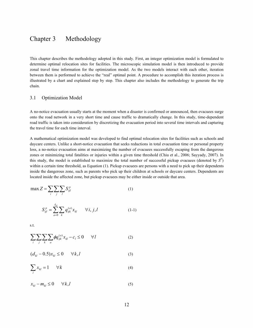
3.1 Optimization Model

A no-notice evacuation usually starts at the moment when a disaster is confirmed or announced, then evacuees surge onto the road network in a very short time and cause traffic to dramatically change. In this study, time-dependent road traffic is taken into consideration by discretizing the evacuation period into several time intervals and capturing the travel time for each time interval.

A mathematical optimization model was developed to find optimal relocation sites for facilities such as schools and daycare centers. Unlike a short-notice evacuation that seeks reductions in total evacuation time or personal property loss, a no-notice evacuation aims at maximizing the number of evacuees successfully escaping from the dangerous zones or minimizing total fatalities or injuries within a given time threshold (Chiu et al., 2006; Sayyady, 2007). In this study, the model is established to maximize the total number of successful pickup evacuees (denoted by SP) within a certain time threshold, as Equation (1). Pickup evacuees are persons with a need to pick up their dependents inside the dangerous zone, such as parents who pick up their children at schools or daycare centers. Dependents are located inside the affected zone, but pickup evacuees may be either inside or outside that area.

i j l

pijlSZmax (1)

ljixqSijlA

a kkl

aijk

pijl ,,

0

)(

(1-1)

s.t.

lcxq li j k a

kla

ijk 0)( (2)

lkxd klkl ,0)5.0( (3)

kxl

kl 1 (4)

lkmx klkl ,0 (5)

13

lkxkl ,1,0 (6)

Where,

i is an index of pickup evacuees’ origin nodes;

j is an index of pickup evacuees’ destination nodes;

k is an index of current locations of facilities;

l is an index of possible relocation sites for facilities;

a is an index of time interval, ath ;

xkl are binary integer decision variables. xkl = 1, if we assign facility k to site l; 0 otherwise;

pijlS is the number of successful pickup evacuees who originate from i (or arrive at the network at i),

stop at relocation site l to pick up their dependent(s) and evacuate to j, within a certain time threshold;

)(aijkq is the number of pickup evacuees who originate from i at time interval a (or arrive at the

network at i at time interval a), with their dependent(s) at facility k, and evacuate to j;

ijlA is the last time interval during which successful evacuation can be ensured for pickup evacuees

who originate from i (or arrive at the network at i), stop at relocation site l to pick up their dependent(s) and evacuate to j;

cl is the capacity of relocation site l (in persons);

dkl is the distance from facility k to relocation site l;

mkl is a binary indicator. mkl=1 if no main streets across between k and l; 0, otherwise;

Ф is the average number of dependents a pickup evacuee gathers at a facility.

Equation (1-1) calculates that the number of successful pickup evacuees for each i, j, l; pijlS is the number of pickup

evacuees (originating from i and evacuating to j) with dependent(s) relocated to l from all facilities before the last

safe time interval, ijlA . Equation (1) determines the total number of successful pickup evacuees by summating pijlS

over i, j, l. Equation (2) requires the number of dependents relocated to possible site l to be no greater than facility l’s capacity. The average number of dependents for a pickup evacuee is assumed to be the same over all of the facilities. Multiple intermediate stops for a pickup trip are not considered in this study; parents who have more than one dependent in the dangerous zone are assumed to have them in one facility. Equation (3) restricts the relocation site to a walkable distance (0.5 miles) from the original site. Equation (4) guarantees that a facility is assigned to one and only one relocation site. Facilities’ current locations are also treated as possible relocation sites. Equation (5) ensures that students do not cross main roads when they are walking to l. The parameter mkl is 1 if no main roads exist between k and l, and 0 otherwise. This constraint ensures student’s safety and that they do not slow road traffic

14

and thereby increase evacuation time. Equation (6) is a binary variable constraint. The optimization model is discrete; time is divided into several intervals, which are treated as a set of integers and associated with a fixed travel cost, i.e., travel time in this study. Lingo 11.0 is used to solve this linear program.

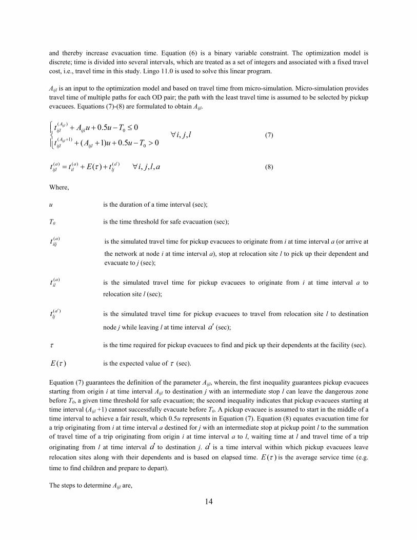
Aijl is an input to the optimization model and based on travel time from micro-simulation. Micro-simulation provides travel time of multiple paths for each OD pair; the path with the least travel time is assumed to be selected by pickup evacuees. Equations (7)-(8) are formulated to obtain Aijl.

ljiTuuAt

TuuAt

ijlA

ijl

ijlA

ijl

ijl

ijl

,,05.0)1(

05.0

0)1(

0)(

(7)

aljitEtt alj

ail

aijl ,,,)( )()()( (8)

Where,

u is the duration of a time interval (sec);

T0 is the time threshold for safe evacuation (sec);

)(ailjt is the simulated travel time for pickup evacuees to originate from i at time interval a (or arrive at

the network at node i at time interval a), stop at relocation site l to pick up their dependent and evacuate to j (sec);

)(ailt is the simulated travel time for pickup evacuees to originate from i at time interval a to

relocation site l (sec);

)(aljt

is the simulated travel time for pickup evacuees to travel from relocation site l to destination

node j while leaving l at time interval a (sec);

is the time required for pickup evacuees to find and pick up their dependents at the facility (sec).

)(E is the expected value of (sec).

Equation (7) guarantees the definition of the parameter Aijl, wherein, the first inequality guarantees pickup evacuees starting from origin i at time interval Aijl to destination j with an intermediate stop l can leave the dangerous zone before T0, a given time threshold for safe evacuation; the second inequality indicates that pickup evacuees starting at time interval (Aijl +1) cannot successfully evacuate before T0. A pickup evacuee is assumed to start in the middle of a time interval to achieve a fair result, which 0.5u represents in Equation (7). Equation (8) equates evacuation time for a trip originating from i at time interval a destined for j with an intermediate stop at pickup point l to the summation of travel time of a trip originating from origin i at time interval a to l, waiting time at l and travel time of a trip

originating from l at time interval a to destination j. a is a time interval within which pickup evacuees leave

relocation sites along with their dependents and is based on elapsed time. )(E is the average service time (e.g.

time to find children and prepare to depart).

The steps to determine Aijl are,

15

1. Set a = M-1. M is the total number of time intervals of [0~T0]. For instance, if T0 is one hour and a time interval is 2.5 minutes, 24 time intervals exist, so M=24 and a ranges from 0 to 23.

2. Calculate uuAt ijlA

ijlijl 5.0)( by substituting Aijl with a; if it is less than T0, which means that

05.0 0)( TuuAt ijl

Aijl

ijl is true, then let Aijl=a, and stop; otherwise, let a = a -1, repeat step 2.

Some pickup evacuees may arrive at relocation sites early and wait for their dependents. This waiting time is not accounted for in the calculation of Aijl, and will not significantly affect the result, because the optimization model includes a 0.5-mile walking distance constraint, which is equally a 10-minute walking time constraint if an average walking speed of 3mph is assumed. People arriving at a relocation site within 10 minutes after the evacuation starts would be able to evacuate safely according to the safe time thresholds investigated here.

3.2 Traffic Simulation Model

Microscopic simulation outputs travel time among origins, destinations, and facility/relocation sites for the optimization model. Micro-simulation was chosen instead of simulation models on other levels, because it can model the road network in great detail, has the ability to model queues, and reflects the impacts of facilities’ entry/exit configuration on travel time, which is crucial for the special case here. VISSIM, part of the PTV VISION traffic analysis package, was used in this study. VISSIM is a driver behavior based, second by second microscopic traffic simulation program, and developed to model major elements of transportation systems, such as lane configuration, vehicle composition, driver behavior, traffic controls and so on (PTV AG, 2005). VISSIM is able to model capacities of parking lots; it can model the situation where a vehicle arrives at a parking lot that is currently full and has to wait outside until someone in the parking lot leaves and empties a space. This ability helps capture abnormal travel time to/from a facility when plenty of vehicles arrive within a very short time period and cause queues and extra travel time. This is one of reasons that VISSIM was chosen to be traffic simulator.

VISSIM’s built-in dynamic traffic assignment algorithm was used to find routes for pickup evacuees. VISSIM accomplishes dynamic assignment procedures by iterated simulation runs. For each iterated run, drivers make decisions on route choice based on road traffic situations they experienced from the previous iterations. After multiple simulation runs, the iterations end when network traffic reaches stability, defined in VISSIM as when travel times or volumes do not vary significantly between two consecutive runs (PTV AG, 2005). The path evaluation file outputs results of the dynamic assignment procedures in a user-defined format (PTV AG, 2005), and was used here to output zonal travel time for pickup evacuees.

3.3 Framework

The road traffic situation determines optimal relocation sites; reversely, relocation sites affect road traffic. In this study, relocation sites are determined by the optimization model and the network traffic is modeled using the simulation model, VISSIM. The optimization model uses travel time output from VISSIM, which assumes current facility locations as pickup points at the beginning. When the optimization model finds new relocation sites, travel time from VISSIM should be updated accordingly; as a result, these determined optimal sites may not be “real”. In order to achieve “real” optimal sites, iteration between the two models is performed until convergence is reached. A procedure to accomplish this iteration process is shown in Figure 1, and executed in C++. At every iteration, new relocation sites are found, and the travel time corresponding to those new sites is updated.

16

Figure 1 Flowchart of the Study

In this procedure, first, the road network under normal conditions is simulated in VISSIM and normal travel times are achieved and adopted by the optimization model to be initial travel time. Then, micro simulation for emergency situations is iteratively executed with the optimization model until the termination criteria are satisfied, to determine optimal relocation sites. Facility current locations are set to be initial pickup locations; during each iteration, new relocation sites are found, and the travel time corresponding to those new sites is updated accordingly.

The procedure follows the steps below:

Initial {xkl}

Generate pickup trip chain

Traffic Simulation in VISSIM

Optimization Model

and output { klx } and

Objective Z

)( aijkq

Update )(ailjt for klx =1

Termination criteria?

{ klx }={ klx }

Output { klx }

End

Generate dummy trips

Traffic simulation in VISSIM

Output {til}, {tlj}

No

Yes

Calculate Aijl

Calculate SP

for { klx }

17

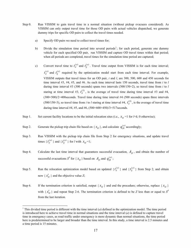
Step 0. Run VISSIM to gain travel time in a normal situation (without pickup evacuees considered). As VISSIM can only output travel time for those OD pairs with actual vehicles dispatched, we generate dummy trips for specific OD pairs to collect the travel times needed.

a) Specify OD pairs we need to collect travel times for;

b) Divide the simulation time period into several periods1; for each period, generate one dummy vehicle for each specified OD pair, run VISSIM and capture OD travel times within that period; when all periods are completed, travel times for the simulation time period are captured;

c) Convert travel time to )(ailt and )(a

ljt . Travel time output from VISSIM is for each time interval;

)(ailt and )(a

ljt required by the optimization model start from each time interval. For example,

VISSIM outputs that travel times for an OD pair, i and l, are 300, 500, 600 and 450 seconds for time interval #3, #4, #5, and #6. As each time interval lasts 150 seconds, travel time from i to l during time interval #3 (300 seconds) spans two intervals (300/150=2), so travel time from i to l

staring at time interval #3, )3(ilt , is the average of travel time during time interval #3 and #4,

(300+500)/2=400seconds. Travel time during time interval #4 (500 seconds) spans three intervals

(500/150≈3), so travel time from i to l staring at time interval #4, )4(ilt , is the average of travel time

during time interval #4, #5, and #6, (500+600+450)/3=517seconds.

Step 1. Set current facility locations to be the initial relocation sites (i.e., klx =1 for l=k; 0 otherwise);

Step 2. Generate the pickup trip chain file based on { klx }, and calculate )(aijkq accordingly;

Step 3. Run VISSIM with the pickup trip chain file from Step 2 for emergency situations, and update travel

times { )(ailt } and { )(a

ljt } for l with klx =1;

Step 4. Calculate the last time interval that guarantees successful evacuation, ijlA , and obtain the number of

successful evacuations SP for { klx } based on ijlA and )(aijkq ;

Step 5. Run the relocation optimization model based on updated { )(ailt } and { )(a

ljt } from Step 2, and obtain

new { klx } and the objective value Z;

Step 6. If the termination criterion is satisfied, output { klx } and end the procedure; otherwise, replace { klx }

with { klx } and repeat Step 2-6. The termination criterion is defined to be Z less than or equal to SP

from the last iteration.

1 This divided time period is different with the time interval (a) defined in the optimization model. The time period is introduced here to achieve travel time in normal situations and the time interval (a) is defined to capture travel time in emergency cases, as road traffic under emergency is more dynamic than normal situations, the time period here is predetermined to be larger and broader than the time interval. In this study, a time interval is 2.5 minutes and a time period is 15 minutes.

18

3.4 Pickup Trip Generation

Pickup trip generation includes determining: 1) the number of pickup evacuees (i.e., parents), 2) their origins and destinations, and 3) the time they arrive at the network. In this study, all dependents at facilities are assumed to be picked up by their families with private cars; no school buses or public transit are assumed to be available for pick up. Thus, pickup demand can be calculated according to the number of dependents in the facilities.

This study focuses on day time evacuation, when household dependents are in facilities like schools or daycare centers and their parents are most likely at work or home. Pickup demand origins (i.e., where parents start at the moment of a disaster) follow a logical assumption by considering where the study area is located from a major business area, i.e., central business district (CBD). Pickup demand destination zones are selected by considering the spatial relations between the disaster location and pickup points. Pickup arrival time is assumed to follow the Normal distribution. Pickup demand in this study is assumed to be deterministic and does not change with road traffic. Different number of pickup demand and different arrival time distributions were tested as sensitivity analysis in Section 4.6.

19

Chapter 4 Case Study

This chapter applies the methodology presented in Chapter 3 to a case study based in Chicago Heights, Cook County, Illinois.

4.1 Network Description

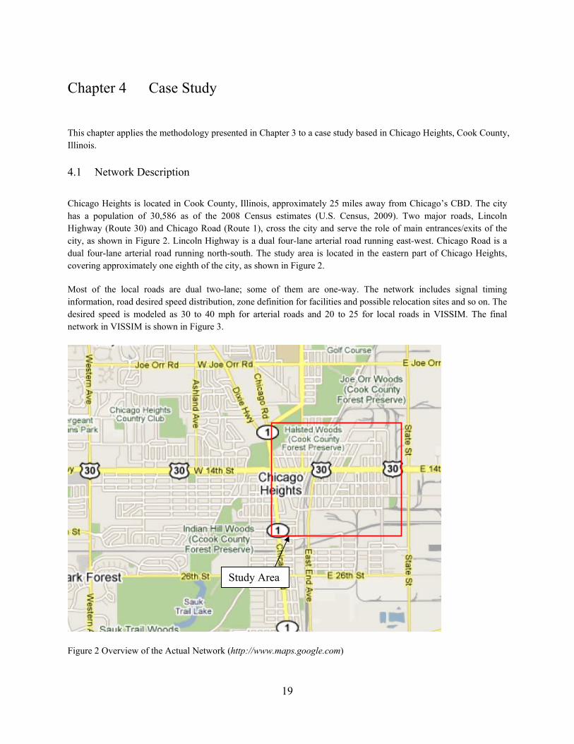
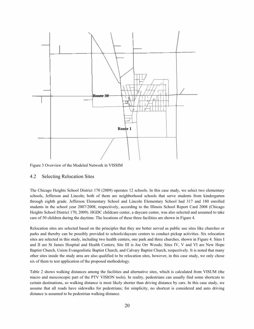
Chicago Heights is located in Cook County, Illinois, approximately 25 miles away from Chicago’s CBD. The city has a population of 30,586 as of the 2008 Census estimates (U.S. Census, 2009). Two major roads, Lincoln Highway (Route 30) and Chicago Road (Route 1), cross the city and serve the role of main entrances/exits of the city, as shown in Figure 2. Lincoln Highway is a dual four-lane arterial road running east-west. Chicago Road is a dual four-lane arterial road running north-south. The study area is located in the eastern part of Chicago Heights, covering approximately one eighth of the city, as shown in Figure 2.

Most of the local roads are dual two-lane; some of them are one-way. The network includes signal timing information, road desired speed distribution, zone definition for facilities and possible relocation sites and so on. The desired speed is modeled as 30 to 40 mph for arterial roads and 20 to 25 for local roads in VISSIM. The final network in VISSIM is shown in Figure 3.

Figure 2 Overview of the Actual Network (http://www.maps.google.com)

Study Area

20

Figure 3 Overview of the Modeled Network in VISSIM

4.2 Selecting Relocation Sites

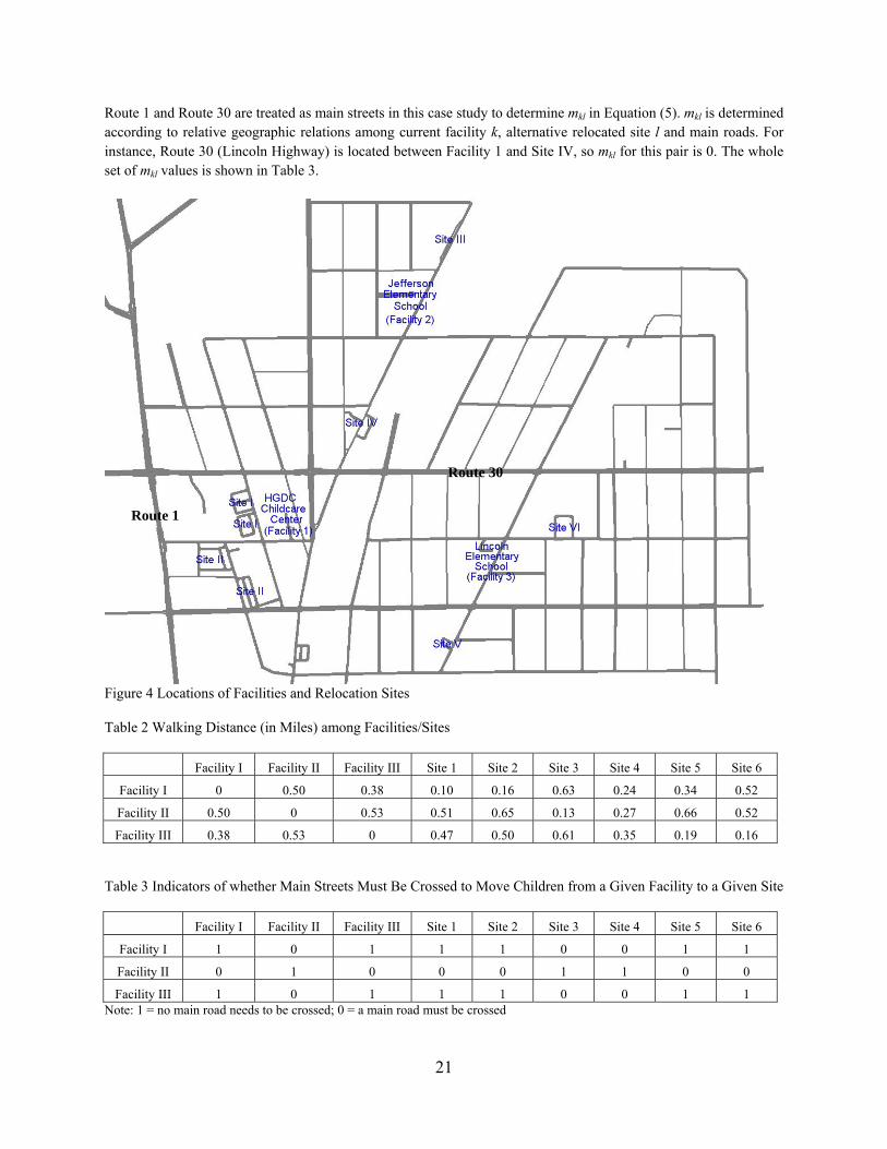
The Chicago Heights School District 170 (2009) operates 12 schools. In this case study, we select two elementary schools, Jefferson and Lincoln; both of them are neighborhood schools that serve students from kindergarten through eighth grade. Jefferson Elementary School and Lincoln Elementary School had 317 and 180 enrolled students in the school year 2007/2008, respectively, according to the Illinois School Report Card 2008 (Chicago Heights School District 170, 2009). HGDC childcare center, a daycare center, was also selected and assumed to take care of 50 children during the daytime. The locations of these three facilities are shown in Figure 4.

Relocation sites are selected based on the principles that they are better served as public use sites like churches or parks and thereby can be possibly provided to schools/daycare centers to conduct pickup activities. Six relocation sites are selected in this study, including two health centers, one park and three churches, shown in Figure 4. Sites I and II are St James Hospital and Health Centers; Site III is Joe Orr Woods; Sites IV, V and VI are New Hope Baptist Church, Union Evangenlistic Baptist Church, and Calvary Baptist Church, respectively. It is noted that many other sites inside the study area are also qualified to be relocation sites, however, in this case study, we only chose six of them to test application of the proposed methodology.

Table 2 shows walking distances among the facilities and alternative sites, which is calculated from VISUM (the macro and mescoscopic part of the PTV VISION tools). In reality, pedestrians can usually find some shortcuts to certain destinations, so walking distance is most likely shorter than driving distance by cars. In this case study, we assume that all roads have sidewalks for pedestrians; for simplicity, no shortcut is considered and auto driving distance is assumed to be pedestrian walking distance.

Route 30

Route 1

21

Route 1 and Route 30 are treated as main streets in this case study to determine mkl in Equation (5). mkl is determined according to relative geographic relations among current facility k, alternative relocated site l and main roads. For instance, Route 30 (Lincoln Highway) is located between Facility 1 and Site IV, so mkl for this pair is 0. The whole set of mkl values is shown in Table 3.

Figure 4 Locations of Facilities and Relocation Sites

Table 2 Walking Distance (in Miles) among Facilities/Sites

Facility I Facility II Facility III Site 1 Site 2 Site 3 Site 4 Site 5 Site 6

Facility I 0 0.50 0.38 0.10 0.16 0.63 0.24 0.34 0.52

Facility II 0.50 0 0.53 0.51 0.65 0.13 0.27 0.66 0.52

Facility III 0.38 0.53 0 0.47 0.50 0.61 0.35 0.19 0.16

Table 3 Indicators of whether Main Streets Must Be Crossed to Move Children from a Given Facility to a Given Site

Facility I Facility II Facility III Site 1 Site 2 Site 3 Site 4 Site 5 Site 6

Facility I 1 0 1 1 1 0 0 1 1

Facility II 0 1 0 0 0 1 1 0 0

Facility III 1 0 1 1 1 0 0 1 1 Note: 1 = no main road needs to be crossed; 0 = a main road must be crossed

Route 30

Route 1

22

4.3 Evacuation Demand Estimation

Travel demand under emergency conditions is composed of three parts: travel demand under normal situations (background traffic), non-pickup evacuation demand, and pickup evacuation demand. Travel demand under normal situations is estimated and provided by CMAP. Non-pickup evacuees refer to the population who are in the impacted area when a disaster occurs and do not have to pick up anyone during the evacuation. Non-pickup demand and pickup demand are estimated separately in this study. Non-pickup evacuees originate from inside the dangerous area; pickup evacuees originate from either inside or outside the dangerous zone and have intermediate stops inside the area to pick up their dependents.

4.3.1 Non-pickup Evacuee Estimation

A no-notice disaster usually has immediate and severe consequences. In this case, people do not have time to consider whether or not to evacuate and when to evacuate; the most likely action they will take is following the evacuation guidance if available, or following most people’s actions. So it is reasonable to assume that all people within the impacted area are evacuees and start evacuating at the time the no-notice disaster occurs. Chiu et al. (2007) assumed that all the evacuation flows are loaded into the network at time 0 while modeling no-notice mass evacuation using a dynamic traffic flow optimization model, based on the same reason indicated here. In this study, in order to avoid loading a large amount of vehicles into the network within a very short time period and causing irrational congestion, and, considering that people need time to prepare for evacuation, we assume non-pickup evacuees depart within 10 minutes after the occurrence of a disaster. VISSIM assumes a Poisson arrival distribution within a time interval (PTV AG, 2005).

The number of evacuees without pickup needs is estimated based on the number of employees and the unemployment status from Census data. From Selected Statistics from the 2002 Economic Census (U.S. Census, 2003), we estimate that there are 11,031 employees within the City of Chicago Heights. From 2005-2007 American Community Survey 3-Year Estimates (U.S. Census, 2008), we calculate that 1979 people over the age of 25 are unemployed in Chicago Heights. As the study area covers 1/8 of the city, the number of non-pickup evacuees is assumed to be 1350 ((11031*0.8+2000)/8 ≈ 1350), evenly distributed through the area. We assume 80% of all employees are on duty on a normal workday; others may be on vacation, medical leave, or out-of-town trip business.

In this case study, ten internal zones are created and evenly distributed within the study area, thereby selected to be non-pickup evacuees’ origins by equal chance; each zone has multiple connectors to the local road network. Eight external zones are defined and treated as possible destinations. Based on the assumption that most evacuees would choose near destinations rather than the others, probabilities of each destination chosen for each origin are estimated by assuming that approximately 70% of evacuees would choose close destinations and among alternative close destinations, each is chosen evenly.

4.3.2 Pickup Evacuee Estimation

Pickup evacuees originate from where they are at the moment of disaster occurrence, which could be either outside or inside the affected area. In this study, the affected area is assumed to be a 2 mile radius from the disaster location, thus pickup evacuees are most likely located outside the area. Here we assume 80% of them are outside the dangerous zone and 20% of them are inside when the disaster occurs. Pickup evacuees’ trip distributions are estimated through different procedures for those originating from outside the affected area and those from inside.

For those pickup evacuees originating inside the affected area, the departure time is assumed to follow a normal distribution with a mean of 5 minutes (after disaster occurrence) and a standard deviation of 1.25 minutes. Both origin and destination choice follow a uniform distribution; precisely, origins are assumed to be evenly distributed

23

among internal zones of the network, and destinations are assumed to be evenly distributed among external zones of the network.

For those pickup evacuees originating outside the affected area, it is important to determine the time they arrive at the network instead of when they actually depart. Arrival time is assumed here to follow a Normal distribution with a mean of 20 minutes and a standard deviation of 5 minutes. (Other parameters for the Normal distribution are tested in Section 4.6 - Sensitivity Analysis.) Destination choice follows a uniform distribution. Origins are determined according to the assumption that 80% of pickup evacuees who depart from outside the affected area are from the Chicago CBD direction.

As mentioned in the previous chapter, the number of pickup evacuees is determined by the total number of dependents in facilities. In this case study, there are totally 547 dependents. One pickup evacuee is assumed to be responsible for 1.11 dependents on average, i.e., Ф=1.11. In addition, the time required for a parent to find and pick up his/her dependents, µ, is assumed to follow a Normal distribution with a mean of 90 seconds and a standard deviation of 20 seconds.

4.4 Other Assumptions and Modeling Considerations

Other assumptions and modeling considerations employed in this case study include:

The VISSIM simulation includes a 600-second warm up period, which is introduced to fill in the empty network at the beginning of the simulation in order to obtain realistic results. The whole simulation period is from 10:50 a.m. to 12:00 p.m., wherein 10:50 a.m.-11:00 a.m. is the warm-up period. A no-notice disaster is assumed to occur at 11:00 a.m., and an evacuation starts immediately. Travel time is updated every 150 seconds in VISSIM.

Parents may arrive at relocation sites earlier than their children and have to wait for them. This waiting time is added to calculate departure time of the trip from relocation sites to destinations in the simulation part; and not accounted for in the optimization formulation because those parents arriving earlier most likely can successfully evacuate.

Dependents in facilities are assumed to walk to relocation sites through the shortest path and not interfere with road traffic. Walking speed is assumed to be 3 mph.

Capacities of facilities 1-3 are assumed to be 100, 500, 200 people; the capacity of each relocation site is assumed to be 500 people. These generous assumptions of capacity are made for the purpose that the results can reflect the impacts of the road network on the relocation strategy clearly.

No other transportation modes (e.g., trains, buses or school buses) are considered for evacuation.

No emergency plan regarding signal timing and right of way is executed.

4.5 Result Analysis

VISSIM uses random seeds to reflect stochastic variation of input flow arrival times (PTV AG, 2005). Different random seeds result in different outputs even though inputs are identical. In this case study, three random seeds are tested and measures (such as travel time) are averaged over different random seeds.

24

Several measures of effectiveness (MOEs) are selected to reflect the performance of the relocation strategy from the perspectives of the overall network, non-pickup evacuees, and pickup evacuees. MOEs include total travel time, average speed, total delay time and average delay time per vehicle for pickup evacuees, non-pickup evacuees, background traffic and the overall network. MOEs are measured over the time period [0, T0]; time 0 is defined as the time of the disaster occurrence, which is 11:00 a.m. in this case study (the warm up period is not included for the strategy evaluation). Improvement of a MOE is formulated as Equation (9), where MOEno and MOEafter represent a MOE in the no-relocation case and a MOE in the after-relocation case. Introducing these MOEs and their improvements is mainly for the purpose of indicating whether, how, and to what extent the relocation strategy would contribute to congestion relief. All these MOEs are determined from VISSIM output files directly and indirectly. An increase of SP, formulated as Equation (10), is also a crucial factor to evaluate the effectiveness of the relocation strategy.

Improvement of a MOE = %100

no

noafter

MOE

MOEMOE (9)

Increase of SP= %100no

P

noP

afterP

S

SS (10)

4.5.1 Improvements of MOEs

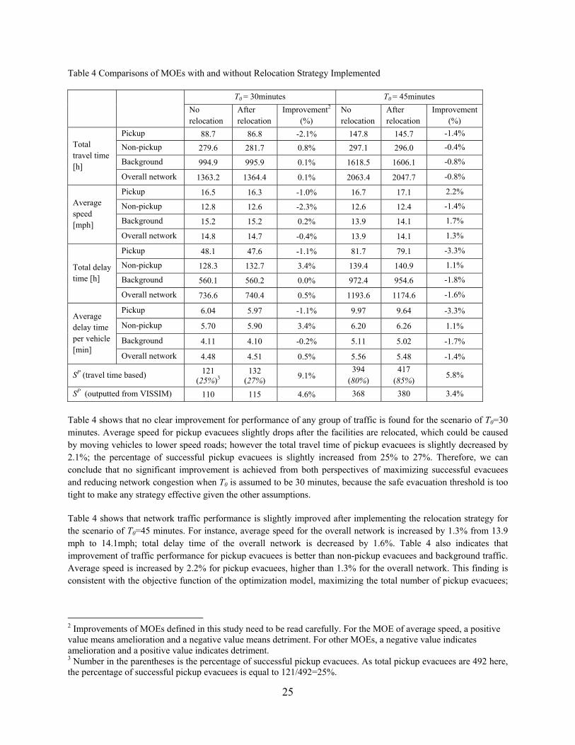
Three safe evacuation time thresholds, 30, 45 and 60 minutes, are tested in this case study. Table 4 includes results of the MOEs for T0 = 30 and 45 minutes. For the scenario of T0=60 minutes, all pickup evacuees can successfully evacuate from the dangerous area without relocation, so no relocation strategy is needed. As shown in Table 4, for the scenario of T0=30 minutes, it was found that the number of successful pickup evacuees can be increased by 11 families (9.1%, calculated over the no relocation scenario) if Facilities 1, 2 and 3 are relocated to Sites I, IV and II, respectively; for the scenario of T0=45minutes, the number of successful pickup evacuees can be increased by 23 families (5.8%) if Facilities 1 and 3 are relocated to Site V and VI, respectively, and Facility 2 remains its current location.

25

Table 4 Comparisons of MOEs with and without Relocation Strategy Implemented

T0 = 30minutes T0 = 45minutes

No relocation

After relocation

Improvement2 (%)

No relocation

After relocation

Improvement (%)

Total travel time [h]

Pickup 88.7 86.8 -2.1% 147.8 145.7 -1.4%

Non-pickup 279.6 281.7 0.8% 297.1 296.0 -0.4%

Background 994.9 995.9 0.1% 1618.5 1606.1 -0.8%

Overall network 1363.2 1364.4 0.1% 2063.4 2047.7 -0.8%

Average speed [mph]

Pickup 16.5 16.3 -1.0% 16.7 17.1 2.2%

Non-pickup 12.8 12.6 -2.3% 12.6 12.4 -1.4%

Background 15.2 15.2 0.2% 13.9 14.1 1.7%

Overall network 14.8 14.7 -0.4% 13.9 14.1 1.3%

Total delay time [h]

Pickup 48.1 47.6 -1.1% 81.7 79.1 -3.3%

Non-pickup 128.3 132.7 3.4% 139.4 140.9 1.1%

Background 560.1 560.2 0.0% 972.4 954.6 -1.8%

Overall network 736.6 740.4 0.5% 1193.6 1174.6 -1.6%

Average delay time per vehicle [min]

Pickup 6.04 5.97 -1.1% 9.97 9.64 -3.3%

Non-pickup 5.70 5.90 3.4% 6.20 6.26 1.1%

Background 4.11 4.10 -0.2% 5.11 5.02 -1.7%

Overall network 4.48 4.51 0.5% 5.56 5.48 -1.4%

SP (travel time based) 121 (25%)3

132 (27%)

9.1% 394

(80%) 417

(85%) 5.8%

SP (outputted from VISSIM) 110 115 4.6% 368 380 3.4%

Table 4 shows that no clear improvement for performance of any group of traffic is found for the scenario of T0=30 minutes. Average speed for pickup evacuees slightly drops after the facilities are relocated, which could be caused by moving vehicles to lower speed roads; however the total travel time of pickup evacuees is slightly decreased by 2.1%; the percentage of successful pickup evacuees is slightly increased from 25% to 27%. Therefore, we can conclude that no significant improvement is achieved from both perspectives of maximizing successful evacuees and reducing network congestion when T0 is assumed to be 30 minutes, because the safe evacuation threshold is too tight to make any strategy effective given the other assumptions.

Table 4 shows that network traffic performance is slightly improved after implementing the relocation strategy for the scenario of T0=45 minutes. For instance, average speed for the overall network is increased by 1.3% from 13.9 mph to 14.1mph; total delay time of the overall network is decreased by 1.6%. Table 4 also indicates that improvement of traffic performance for pickup evacuees is better than non-pickup evacuees and background traffic. Average speed is increased by 2.2% for pickup evacuees, higher than 1.3% for the overall network. This finding is consistent with the objective function of the optimization model, maximizing the total number of pickup evacuees;

2 Improvements of MOEs defined in this study need to be read carefully. For the MOE of average speed, a positive value means amelioration and a negative value means detriment. For other MOEs, a negative value indicates amelioration and a positive value indicates detriment. 3 Number in the parentheses is the percentage of successful pickup evacuees. As total pickup evacuees are 492 here, the percentage of successful pickup evacuees is equal to 121/492=25%.

26

to achieve this objective, the benefits of some other traffic may be scarified, e.g., in this scenario, average speed for non-pickup evacuees is decreased by 1.4% after the relocation strategy is implemented.

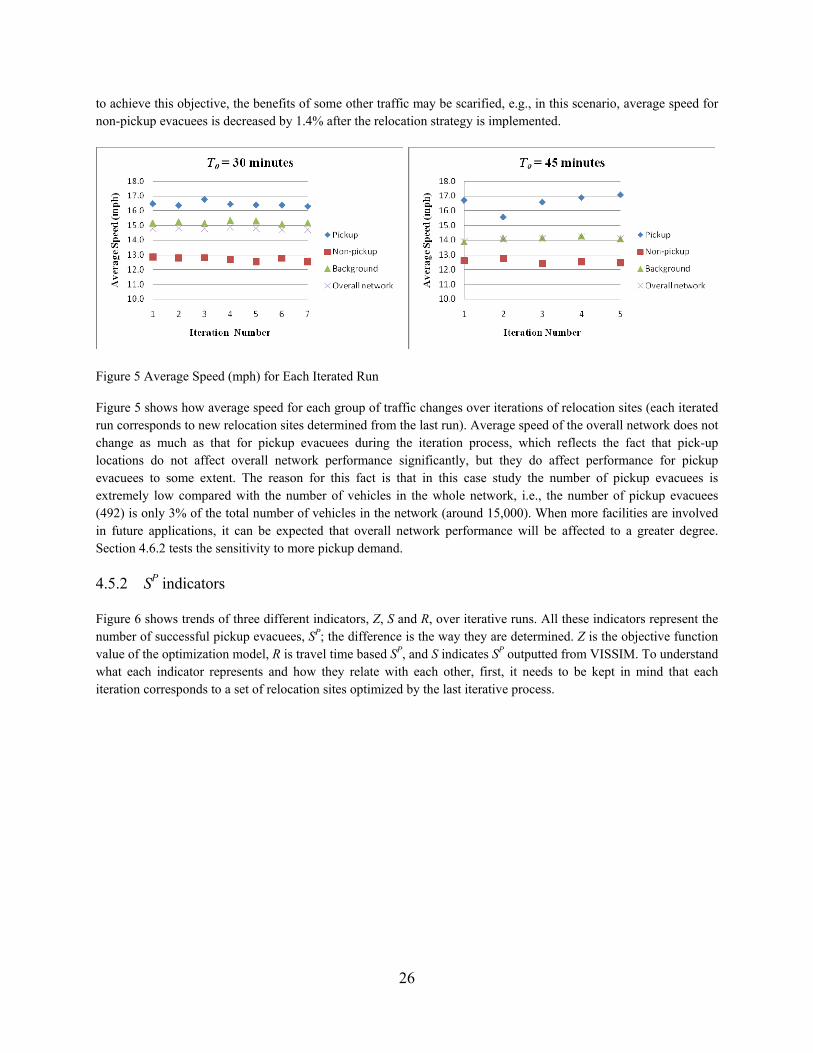
Figure 5 Average Speed (mph) for Each Iterated Run

Figure 5 shows how average speed for each group of traffic changes over iterations of relocation sites (each iterated run corresponds to new relocation sites determined from the last run). Average speed of the overall network does not change as much as that for pickup evacuees during the iteration process, which reflects the fact that pick-up locations do not affect overall network performance significantly, but they do affect performance for pickup evacuees to some extent. The reason for this fact is that in this case study the number of pickup evacuees is extremely low compared with the number of vehicles in the whole network, i.e., the number of pickup evacuees (492) is only 3% of the total number of vehicles in the network (around 15,000). When more facilities are involved in future applications, it can be expected that overall network performance will be affected to a greater degree. Section 4.6.2 tests the sensitivity to more pickup demand.

4.5.2 SP indicators

Figure 6 shows trends of three different indicators, Z, S and R, over iterative runs. All these indicators represent the number of successful pickup evacuees, SP; the difference is the way they are determined. Z is the objective function value of the optimization model, R is travel time based SP, and S indicates SP outputted from VISSIM. To understand what each indicator represents and how they relate with each other, first, it needs to be kept in mind that each iteration corresponds to a set of relocation sites optimized by the last iterative process.

27

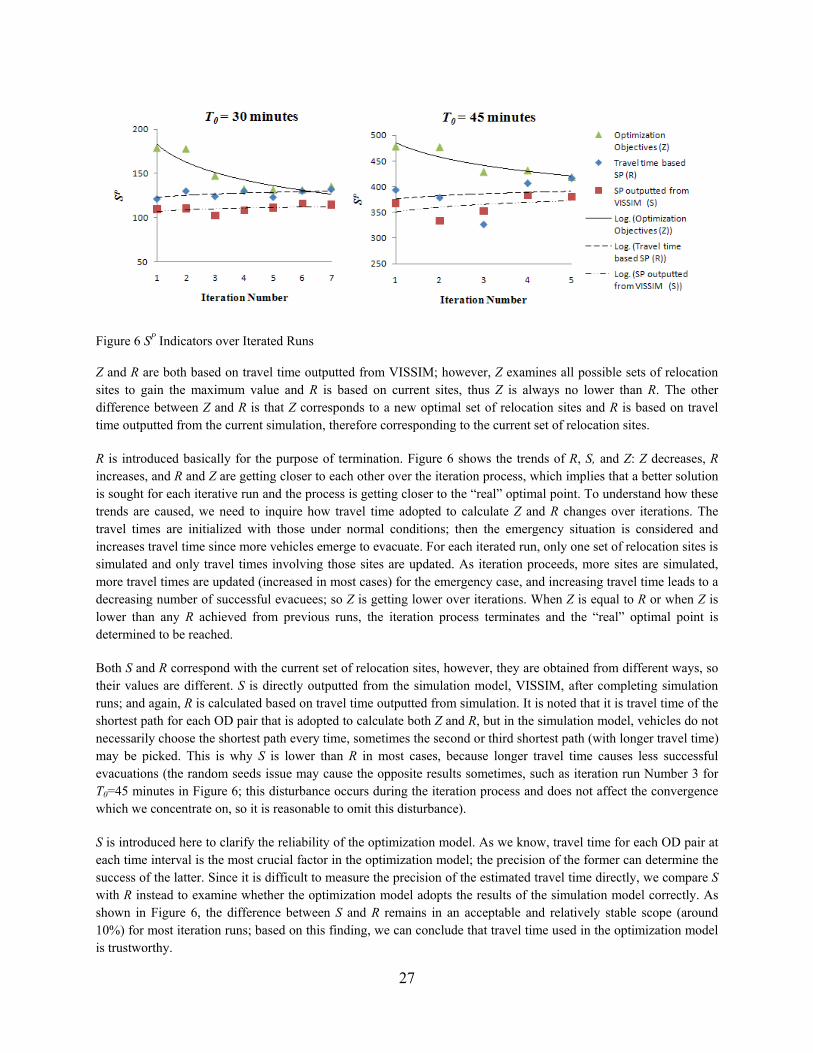
Figure 6 SP Indicators over Iterated Runs

Z and R are both based on travel time outputted from VISSIM; however, Z examines all possible sets of relocation sites to gain the maximum value and R is based on current sites, thus Z is always no lower than R. The other difference between Z and R is that Z corresponds to a new optimal set of relocation sites and R is based on travel time outputted from the current simulation, therefore corresponding to the current set of relocation sites.

R is introduced basically for the purpose of termination. Figure 6 shows the trends of R, S, and Z: Z decreases, R increases, and R and Z are getting closer to each other over the iteration process, which implies that a better solution is sought for each iterative run and the process is getting closer to the “real” optimal point. To understand how these trends are caused, we need to inquire how travel time adopted to calculate Z and R changes over iterations. The travel times are initialized with those under normal conditions; then the emergency situation is considered and increases travel time since more vehicles emerge to evacuate. For each iterated run, only one set of relocation sites is simulated and only travel times involving those sites are updated. As iteration proceeds, more sites are simulated, more travel times are updated (increased in most cases) for the emergency case, and increasing travel time leads to a decreasing number of successful evacuees; so Z is getting lower over iterations. When Z is equal to R or when Z is lower than any R achieved from previous runs, the iteration process terminates and the “real” optimal point is determined to be reached.

Both S and R correspond with the current set of relocation sites, however, they are obtained from different ways, so their values are different. S is directly outputted from the simulation model, VISSIM, after completing simulation runs; and again, R is calculated based on travel time outputted from simulation. It is noted that it is travel time of the shortest path for each OD pair that is adopted to calculate both Z and R, but in the simulation model, vehicles do not necessarily choose the shortest path every time, sometimes the second or third shortest path (with longer travel time) may be picked. This is why S is lower than R in most cases, because longer travel time causes less successful evacuations (the random seeds issue may cause the opposite results sometimes, such as iteration run Number 3 for T0=45 minutes in Figure 6; this disturbance occurs during the iteration process and does not affect the convergence which we concentrate on, so it is reasonable to omit this disturbance).

S is introduced here to clarify the reliability of the optimization model. As we know, travel time for each OD pair at each time interval is the most crucial factor in the optimization model; the precision of the former can determine the success of the latter. Since it is difficult to measure the precision of the estimated travel time directly, we compare S with R instead to examine whether the optimization model adopts the results of the simulation model correctly. As shown in Figure 6, the difference between S and R remains in an acceptable and relatively stable scope (around 10%) for most iteration runs; based on this finding, we can conclude that travel time used in the optimization model is trustworthy.

28

4.6 Sensitivity Analysis

The relocation strategy is very sensitive to many factors, including the safe evacuation time threshold T0 and those regarding pickup evacuees, such as the total number of pickup evacuees, their arriving time and their origin and destination locations. Any change of these factors may result in different sets of relocation sites and different extents to which network traffic performance is improved or deteriorated. The influence of pickup evacuees’ origins and destinations relies on current facility locations and road network configerations, so it is specific for a certain area. As here we are exploring general cases, we choose to investigate sensitivity of the relocation strategy to T0, the total number of pickup evacuees, and their arrival time distribution, and draw some conclusions that can be generally extended to other areas.

Addtionally, we should keep in mind that as the optimization model seeks the optimal point for all invovled facilities, all these facilties’ selected relocation sites interact with each other, in other words, relocating one facility will affect finding sites for other facilities, so there will be a variety of sets of relocation sites changing over different pickup evacuee demand scenarios.

4.6.1 Sensitivity to pickup evacuee arrival time distribution ( , ) and T0

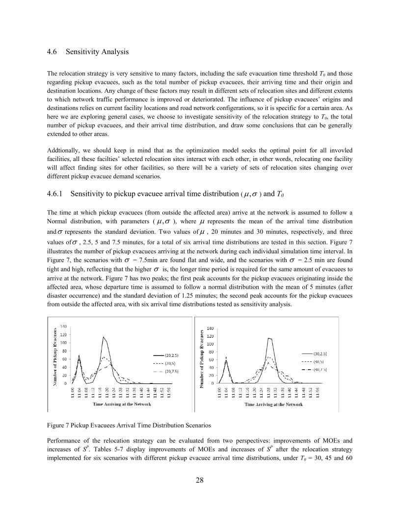
The time at which pickup evacuees (from outside the affected area) arrive at the network is assumed to follow a Normal distribution, with parameters ( , ), where represents the mean of the arrival time distribution

and represents the standard deviation. Two values of , 20 minutes and 30 minutes, respectively, and three

values of , 2.5, 5 and 7.5 minutes, for a total of six arrival time distributions are tested in this section. Figure 7

illustrates the number of pickup evacuees arriving at the network during each individual simulation time interval. In Figure 7, the scenarios with = 7.5min are found flat and wide, and the scenarios with = 2.5 min are found

tight and high, reflecting that the higher is, the longer time period is required for the same amount of evacuees to

arrive at the network. Figure 7 has two peaks; the first peak accounts for the pickup evacuees originating inside the affected area, whose departure time is assumed to follow a normal distribution with the mean of 5 minutes (after disaster occurrence) and the standard deviation of 1.25 minutes; the second peak accounts for the pickup evacuees from outside the affected area, with six arrival time distributions tested as sensitivity analysis.

Figure 7 Pickup Evacuees Arrival Time Distribution Scenarios

Performance of the relocation strategy can be evaluated from two perspectives: improvements of MOEs and increases of SP. Tables 5-7 display improvements of MOEs and increases of SP after the relocation strategy implemented for six scenarios with different pickup evacuee arrival time distributions, under T0 = 30, 45 and 60

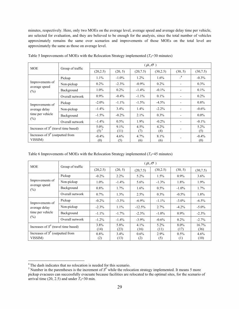
29

minutes, respectively. Here, only two MOEs on the average level, average speed and average delay time per vehicle, are selected for evaluation, and they are believed to be enough for the analysis, since the total number of vehicles approximately remains the same over scenarios and improvements of those MOEs on the total level are approximately the same as those on average level.

Table 5 Improvements of MOEs with the Relocation Strategy implemented (T0=30 minutes)

MOE Group of traffic ( , )

(20,2.5) (20, 5) (20,7.5) (30,2.5) (30, 5) (30,7.5)

Improvements of average speed (%)

Pickup 1.1% -1.0% 1.2% 1.6% -4 -0.3%

Non-pickup 0.2% -2.3% -0.9% 0.2% - 0.3%

Background 1.0% 0.2% -1.4% -0.1% - 0.1%

Overall network 0.9% -0.4% -1.1% 0.1% - 0.2%

Improvements of average delay time per vehicle (%)

Pickup -2.0% -1.1% -1.5% -4.5% - 0.8%

Non-pickup -1.4% 3.4% 1.4% -2.2% - -0.6%

Background -1.5% -0.2% 2.1% 0.3% - 0.0%

Overall network -1.4% 0.5% 1.9% -0.2% - -0.1%

Increases of SP (travel time based) 5.0% (5) 5

9.1% (11)

4.5% (7)

4.2% (4)

- 5.2% (5)

Increases of SP (outputted from VISSIM)

-0.4% (0)

4.6% (5)

4.7% (6)

8.1% (6)

- -0.4% (0)



(20,2.5) (20, 5) (20,7.5) (30,2.5) (30, 5) (30,7.5)


Pickup -0.2% 2.2% 5.2% 1.5% 0.9% 3.6%

Non-pickup 1.0% -1.4% 5.6% -1.3% 1.8% 1.9%

Background 0.8% 1.7% 1.6% 0.5% -1.0% 1.7%

Overall network 0.7% 1.3% 2.5% 0.3% -0.5% 1.8%


Pickup -0.2% -3.3% -6.9% -1.1% -3.0% -6.5%

Non-pickup -2.3% 1.1% -12.5% 2.7% -4.2% -5.0%

Background -1.1% -1.7% -2.3% -1.0% 0.9% -2.3%

Overall network -1.2% -1.4% -3.9% -0.6% 0.2% -2.7%

Increases of SP (travel time based) 3.8% (14)

5.8% (23)

4.1% (16)

5.2% (11)

8.0% (17)

16.7% (36)


0.8% (2)

3.4% (13)

0.6% (2)

2.9% (5)

0.5% (1)

4.6% (10)

4 The dash indicates that no relocation is needed for this scenario. 5 Number in the parentheses is the increment of SP while the relocation strategy implemented. It means 5 more pickup evacuees can successfully evacuate because facilities are relocated to the optimal sites, for the scenario of arrival time (20, 2.5) and under T0=30 min.

30



(20,2.5) (20, 5) (20,7.5) (30,2.5) (30, 5) (30,7.5)


Pickup - - -2.2% 4.8% 2.3% 0.8%

Non-pickup - - -0.6% -2.3% 1.0% -0.5%

Background - - 3.8% 1.7% -1.1% 2.5%

Overall network - - 3.0% 1.5% -0.7% 2.1%


Pickup - - 8.6% -4.8% -3.7% -1.2%

Non-pickup - - -0.7% 3.5% -2.6% 0.3%

Background - - -5.1% -1.9% 1.4% -2.8%

Overall network - - -4.0% -1.4% 0.8% -2.4%

Increases of SP (travel time based) - - 0.2% (1)

1.7% (8)

3.3% (15)

1.1% (5)


- - 0.2% (1)

9.4% (38)

2.2% (10)

1.3% (6)

Improvements of MOEs and increases of SP are not necessarily consistent with each other for a certain scenario. It means a relocation that leads to significant improvements for the network traffic performance does not necessarily cause significant increases of SP. For example, for pickup demand (20, 7.5), when T0=60 minutes, the average speed of the overall network is increased by 3.0% and the average delay time per vehicle is decreased by 4.0%; these improvements can be considered as significant, compared to other scenarios, but SP is only increased by 0.2% and only one more family successfully evacuates after the facilities are relocated. Similarly, a relocation that leads to a significant increase in SP does not necessarily cause significant improvements in network traffic. For instance, for the same pickup demand (20, 7.5), when T0=30 minutes, SP is increased by 4.5%, but performance of overall network is deteriorated by 1-2%.

Improvements of MOEs

Tables 5-7 show that both mean and standard deviation of pickup evacuee arrival time distributions have effects on network traffic improvement caused by facility relocation; in most cases, higher standard deviation and lower mean cause better improvements of network performance by relocating facility dependents. Take the average speed of the overall network as an example: for T0=45 minutes, it is improved by 0.7% after relocation for the scenario of (20, 2.5), higher than 0.3% for the scenario of (30, 2.5), and it is improved by 1.8% for (30, 7.5), higher than 0.3% for (30, 2.5). This finding implies that the relocation strategy gains better performance when pickup evacuees arrive at the network earlier and in a broader period of time; early arrival leaves more time for safe evacuation and a broad arrival time period causes less congestion, both of which are potential reasons why the relocation strategy works better for those situations.

However, the effects of these factors ( and ) on relocation strategy performance are quite tenuous, the safe

evacuation time threshold, T0, is still one of the most significant elements that influences the relocation strategy. When T0 is adequately high, such as 60 minutes for the scenario of (20, 2.5) and (20, 5) in this case study, no relocation strategy is needed; in other cases, the higher T0 is, the more extensive improvements of MOEs can be by implementing the relocation strategy. Take the scenario (30, 7.5) as an example, average speed of the overall network is improved by 2.1%, 1.8%, 0.2% for T0 = 60, 45, and 30 minutes, respectively. This trend could be caused by the fact that within longer time periods of T0, more traffic is involved thus more improvements are obtained.

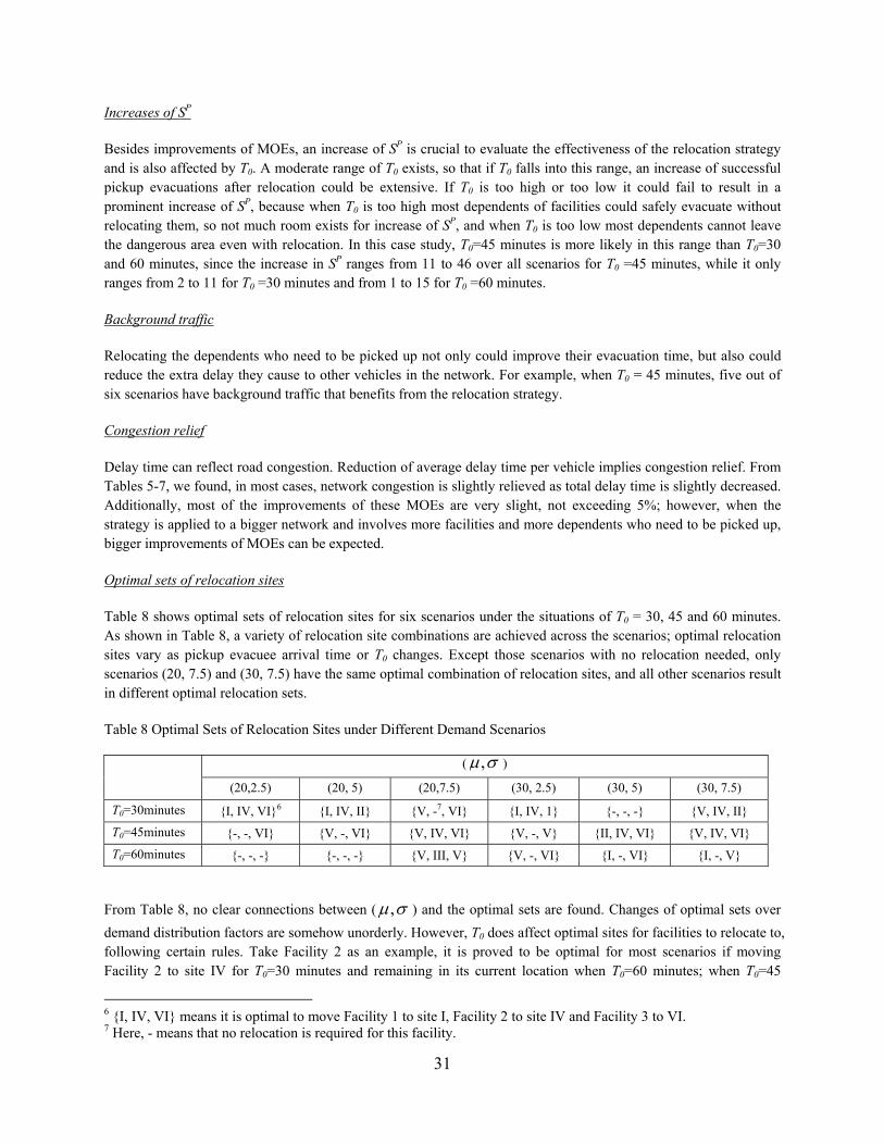
31

Increases of SP

Besides improvements of MOEs, an increase of SP is crucial to evaluate the effectiveness of the relocation strategy and is also affected by T0. A moderate range of T0 exists, so that if T0 falls into this range, an increase of successful pickup evacuations after relocation could be extensive. If T0 is too high or too low it could fail to result in a prominent increase of SP, because when T0 is too high most dependents of facilities could safely evacuate without relocating them, so not much room exists for increase of SP, and when T0 is too low most dependents cannot leave the dangerous area even with relocation. In this case study, T0=45 minutes is more likely in this range than T0=30 and 60 minutes, since the increase in SP ranges from 11 to 46 over all scenarios for T0 =45 minutes, while it only ranges from 2 to 11 for T0 =30 minutes and from 1 to 15 for T0 =60 minutes.

Background traffic

Relocating the dependents who need to be picked up not only could improve their evacuation time, but also could reduce the extra delay they cause to other vehicles in the network. For example, when T0 = 45 minutes, five out of six scenarios have background traffic that benefits from the relocation strategy.

Congestion relief

Delay time can reflect road congestion. Reduction of average delay time per vehicle implies congestion relief. From Tables 5-7, we found, in most cases, network congestion is slightly relieved as total delay time is slightly decreased. Additionally, most of the improvements of these MOEs are very slight, not exceeding 5%; however, when the strategy is applied to a bigger network and involves more facilities and more dependents who need to be picked up, bigger improvements of MOEs can be expected.

Optimal sets of relocation sites

Table 8 shows optimal sets of relocation sites for six scenarios under the situations of T0 = 30, 45 and 60 minutes. As shown in Table 8, a variety of relocation site combinations are achieved across the scenarios; optimal relocation sites vary as pickup evacuee arrival time or T0 changes. Except those scenarios with no relocation needed, only scenarios (20, 7.5) and (30, 7.5) have the same optimal combination of relocation sites, and all other scenarios result in different optimal relocation sets.

Table 8 Optimal Sets of Relocation Sites under Different Demand Scenarios

( , )

(20,2.5) (20, 5) (20,7.5) (30, 2.5) (30, 5) (30, 7.5)

T0=30minutes {I, IV, VI}6 {I, IV, II} {V, -7, VI} {I, IV, 1} {-, -, -} {V, IV, II}

T0=45minutes {-, -, VI} {V, -, VI} {V, IV, VI} {V, -, V} {II, IV, VI} {V, IV, VI}

T0=60minutes {-, -, -} {-, -, -} {V, III, V} {V, -, VI} {I, -, VI} {I, -, V}

From Table 8, no clear connections between ( , ) and the optimal sets are found. Changes of optimal sets over

demand distribution factors are somehow unorderly. However, T0 does affect optimal sites for facilities to relocate to, following certain rules. Take Facility 2 as an example, it is proved to be optimal for most scenarios if moving Facility 2 to site IV for T0=30 minutes and remaining in its current location when T0=60 minutes; when T0=45

6 {I, IV, VI} means it is optimal to move Facility 1 to site I, Facility 2 to site IV and Facility 3 to VI. 7 Here, - means that no relocation is required for this facility.

32

minutes, Facility 2 is either relocated to site IV or remains its current location by equal chance over the six demand scenarios. However, no clear rules are found for the other two facilities. Facilities 1 and 3 tend to have sites V and VI as their optimal sites for T0=45 minutes, respectively; but no dominating optimal site exists for them when T0 = 30 and 60 minutes. The possible reason that Facility 2 has a clear tendency for relocation sites to change over T0 but the other two facilities do not is because Facility 2 has many more dependents (317) than the others (50 and 180).

From Table 8, optimal sets of relocation sites show diversity over scenarios. Unfortunately, this is not feasible for applying to reality. Additionally, by running these scenarios, it is found that the determined “optimal” set may not be significantly better than the second or third optimal set found during the iteration process; sometimes the differences between them are quite slight (see Figures 5 and 6-T0=30 minutes), and in some cases the optimal sets exist because several sets provide the same results (alternative optima). Therefore, for the purpose of practical application, and considering that the determined “optimal” set is not necessarily significantly more advantageous than some others, we generalize Table 8 and present the recommended optimal set(s).

As T0 affects optimal sets of relocation sites, we here recommend relocation sites for each T0 individually. According to the findings from Table 8, we suggest {V, IV, VI} to be relocation sites of Facility {1, 2, 3} for T0=30 minutes, {V, IV, VI} for T0=45 minutes and {V, -, VI} for T0=60 minutes. In section 4.7, these recommended sets are tested and compared with the optimal ones found here.

4.6.2 Sensitivity to total number of pickup evacuees

This case study only involves 3 facilities and a total of 492 pickup evacuees, which is a small number compared with approximately 15,000 vehicles of background traffic. This is one of the possible reasons why all scenarios only result in slight improvements of MOEs and increases of SP. In order to examine the influence of scale of pickup demand on performance of the relocation strategy, we here increase the total pickup demand by 50% and test it with the scenario of (20, 2.5) and (20, 5). Improvements of MOEs are compared between original demand and increased demand, shown in Tables 9-10.

Table 9 Comparisons of Improvements of MOEs between Original Demand and Increased Demand (20, 2.5)

MOE Group of traffic

T0 (minutes)

30 45 60

Original demand

Increased demand

Original demand

Increased demand

Original demand

Increased demand


Pickup 1.1% 2.8% -0.2% 10.8% - 8.1%

Non-pickup 0.2% -3.1% 1.0% 1.4% - 1.5%

Background 1.0% 1.5% 0.8% -0.3% - -0.8%

Overall network 0.9% 0.7% 0.7% 1.0% - 0.4%


Pickup -2.0% -3.0% -0.2% -2.8% - -1.4%

Non-pickup -1.4% 5.6% -2.3% -1.5% - -1.7%

Background -1.5% -2.1% -1.1% 0.7% - 0.8%

Overall network -1.4% -0.6% -1.2% 0.2% - 0.3%


5.3% (7)

3.8% (14)

34.0% (128)

- 32.9% (178)


-0.4% (0)

6.8% (7)

0.8% (2)

15.6% (53)

- 29.4% (130)

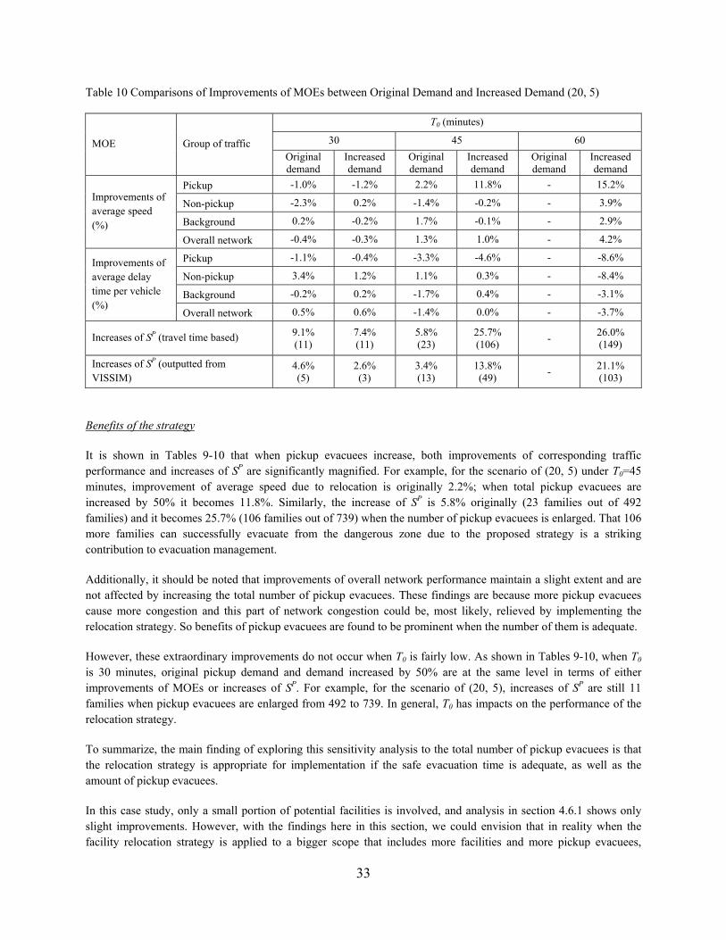
33

Table 10 Comparisons of Improvements of MOEs between Original Demand and Increased Demand (20, 5)

MOE Group of traffic

T0 (minutes)

30 45 60

Original demand

Increased demand

Original demand

Increased demand

Original demand

Increased demand


Pickup -1.0% -1.2% 2.2% 11.8% - 15.2%

Non-pickup -2.3% 0.2% -1.4% -0.2% - 3.9%

Background 0.2% -0.2% 1.7% -0.1% - 2.9%

Overall network -0.4% -0.3% 1.3% 1.0% - 4.2%


Pickup -1.1% -0.4% -3.3% -4.6% - -8.6%

Non-pickup 3.4% 1.2% 1.1% 0.3% - -8.4%

Background -0.2% 0.2% -1.7% 0.4% - -3.1%

Overall network 0.5% 0.6% -1.4% 0.0% - -3.7%


7.4% (11)

5.8% (23)

25.7% (106)

- 26.0% (149)


4.6% (5)

2.6% (3)

3.4% (13)

13.8% (49)

- 21.1% (103)

Benefits of the strategy

It is shown in Tables 9-10 that when pickup evacuees increase, both improvements of corresponding traffic performance and increases of SP are significantly magnified. For example, for the scenario of (20, 5) under T0=45 minutes, improvement of average speed due to relocation is originally 2.2%; when total pickup evacuees are increased by 50% it becomes 11.8%. Similarly, the increase of SP is 5.8% originally (23 families out of 492 families) and it becomes 25.7% (106 families out of 739) when the number of pickup evacuees is enlarged. That 106 more families can successfully evacuate from the dangerous zone due to the proposed strategy is a striking contribution to evacuation management.

Additionally, it should be noted that improvements of overall network performance maintain a slight extent and are not affected by increasing the total number of pickup evacuees. These findings are because more pickup evacuees cause more congestion and this part of network congestion could be, most likely, relieved by implementing the relocation strategy. So benefits of pickup evacuees are found to be prominent when the number of them is adequate.

However, these extraordinary improvements do not occur when T0 is fairly low. As shown in Tables 9-10, when T0 is 30 minutes, original pickup demand and demand increased by 50% are at the same level in terms of either improvements of MOEs or increases of SP. For example, for the scenario of (20, 5), increases of SP are still 11 families when pickup evacuees are enlarged from 492 to 739. In general, T0 has impacts on the performance of the relocation strategy.

To summarize, the main finding of exploring this sensitivity analysis to the total number of pickup evacuees is that the relocation strategy is appropriate for implementation if the safe evacuation time is adequate, as well as the amount of pickup evacuees.

In this case study, only a small portion of potential facilities is involved, and analysis in section 4.6.1 shows only slight improvements. However, with the findings here in this section, we could envision that in reality when the facility relocation strategy is applied to a bigger scope that includes more facilities and more pickup evacuees,

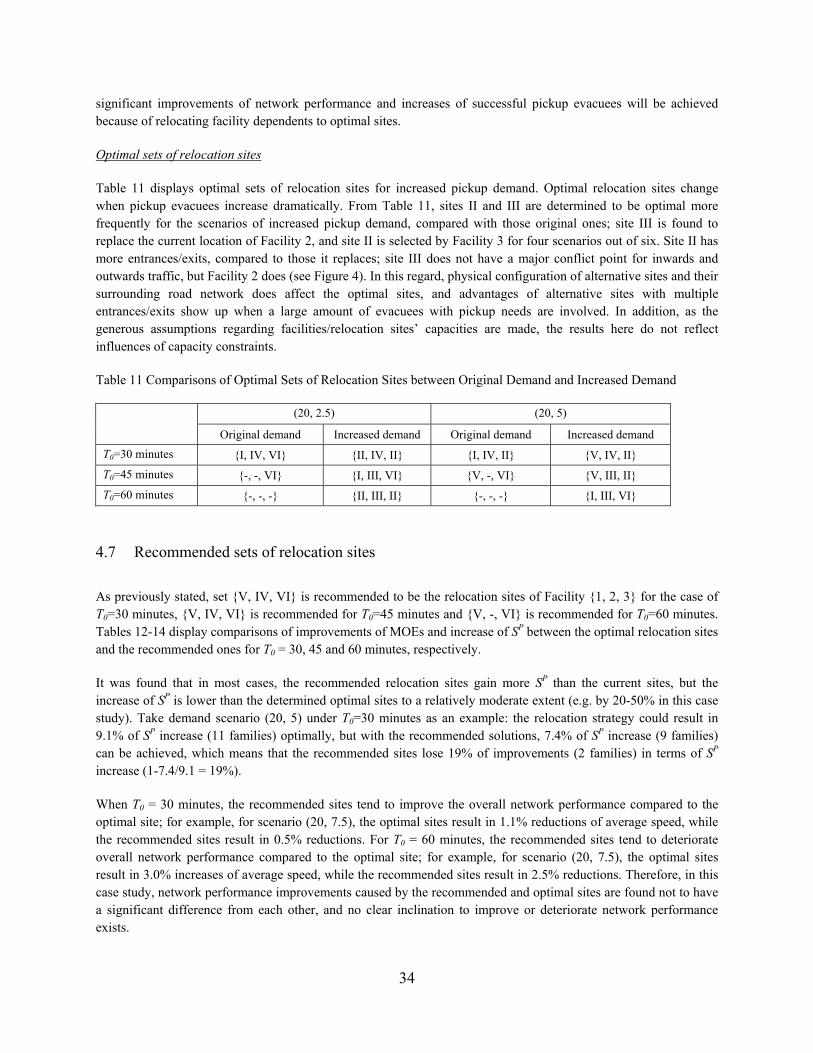
34

significant improvements of network performance and increases of successful pickup evacuees will be achieved because of relocating facility dependents to optimal sites.

Optimal sets of relocation sites

Table 11 displays optimal sets of relocation sites for increased pickup demand. Optimal relocation sites change when pickup evacuees increase dramatically. From Table 11, sites II and III are determined to be optimal more frequently for the scenarios of increased pickup demand, compared with those original ones; site III is found to replace the current location of Facility 2, and site II is selected by Facility 3 for four scenarios out of six. Site II has more entrances/exits, compared to those it replaces; site III does not have a major conflict point for inwards and outwards traffic, but Facility 2 does (see Figure 4). In this regard, physical configuration of alternative sites and their surrounding road network does affect the optimal sites, and advantages of alternative sites with multiple entrances/exits show up when a large amount of evacuees with pickup needs are involved. In addition, as the generous assumptions regarding facilities/relocation sites’ capacities are made, the results here do not reflect influences of capacity constraints.

Table 11 Comparisons of Optimal Sets of Relocation Sites between Original Demand and Increased Demand

(20, 2.5) (20, 5)

Original demand Increased demand Original demand Increased demand

T0=30 minutes {I, IV, VI} {II, IV, II} {I, IV, II} {V, IV, II}

T0=45 minutes {-, -, VI} {I, III, VI} {V, -, VI} {V, III, II}

T0=60 minutes {-, -, -} {II, III, II} {-, -, -} {I, III, VI}

4.7 Recommended sets of relocation sites

As previously stated, set {V, IV, VI} is recommended to be the relocation sites of Facility {1, 2, 3} for the case of T0=30 minutes, {V, IV, VI} is recommended for T0=45 minutes and {V, -, VI} is recommended for T0=60 minutes. Tables 12-14 display comparisons of improvements of MOEs and increase of SP between the optimal relocation sites and the recommended ones for T0 = 30, 45 and 60 minutes, respectively.

It was found that in most cases, the recommended relocation sites gain more SP than the current sites, but the increase of SP is lower than the determined optimal sites to a relatively moderate extent (e.g. by 20-50% in this case study). Take demand scenario (20, 5) under T0=30 minutes as an example: the relocation strategy could result in 9.1% of SP increase (11 families) optimally, but with the recommended solutions, 7.4% of SP increase (9 families) can be achieved, which means that the recommended sites lose 19% of improvements (2 families) in terms of SP increase (1-7.4/9.1 = 19%).

When T0 = 30 minutes, the recommended sites tend to improve the overall network performance compared to the optimal site; for example, for scenario (20, 7.5), the optimal sites result in 1.1% reductions of average speed, while the recommended sites result in 0.5% reductions. For T0 = 60 minutes, the recommended sites tend to deteriorate overall network performance compared to the optimal site; for example, for scenario (20, 7.5), the optimal sites result in 3.0% increases of average speed, while the recommended sites result in 2.5% reductions. Therefore, in this case study, network performance improvements caused by the recommended and optimal sites are found not to have a significant difference from each other, and no clear inclination to improve or deteriorate network performance exists.

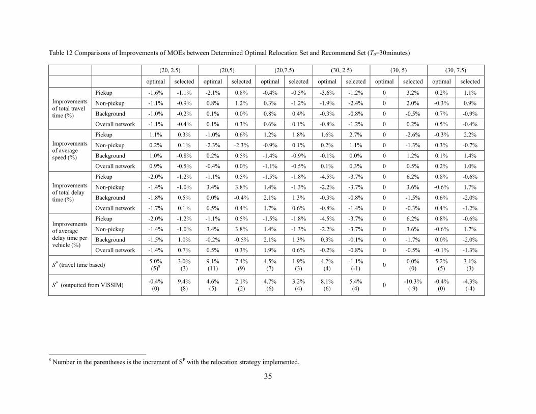
35

Table 12 Comparisons of Improvements of MOEs between Determined Optimal Relocation Set and Recommend Set (T0=30minutes)

(20, 2.5) (20,5) (20,7.5) (30, 2.5) (30, 5) (30, 7.5)

optimal selected optimal selected optimal selected optimal selected optimal selected optimal selected

Improvements of total travel time (%)

Pickup -1.6% -1.1% -2.1% 0.8% -0.4% -0.5% -3.6% -1.2% 0 3.2% 0.2% 1.1%

Non-pickup -1.1% -0.9% 0.8% 1.2% 0.3% -1.2% -1.9% -2.4% 0 2.0% -0.3% 0.9%

Background -1.0% -0.2% 0.1% 0.0% 0.8% 0.4% -0.3% -0.8% 0 -0.5% 0.7% -0.9%

Overall network -1.1% -0.4% 0.1% 0.3% 0.6% 0.1% -0.8% -1.2% 0 0.2% 0.5% -0.4%


Pickup 1.1% 0.3% -1.0% 0.6% 1.2% 1.8% 1.6% 2.7% 0 -2.6% -0.3% 2.2%

Non-pickup 0.2% 0.1% -2.3% -2.3% -0.9% 0.1% 0.2% 1.1% 0 -1.3% 0.3% -0.7%

Background 1.0% -0.8% 0.2% 0.5% -1.4% -0.9% -0.1% 0.0% 0 1.2% 0.1% 1.4%

Overall network 0.9% -0.5% -0.4% 0.0% -1.1% -0.5% 0.1% 0.3% 0 0.5% 0.2% 1.0%

Improvements of total delay time (%)

Pickup -2.0% -1.2% -1.1% 0.5% -1.5% -1.8% -4.5% -3.7% 0 6.2% 0.8% -0.6%

Non-pickup -1.4% -1.0% 3.4% 3.8% 1.4% -1.3% -2.2% -3.7% 0 3.6% -0.6% 1.7%

Background -1.8% 0.5% 0.0% -0.4% 2.1% 1.3% -0.3% -0.8% 0 -1.5% 0.6% -2.0%

Overall network -1.7% 0.1% 0.5% 0.4% 1.7% 0.6% -0.8% -1.4% 0 -0.3% 0.4% -1.2%


Pickup -2.0% -1.2% -1.1% 0.5% -1.5% -1.8% -4.5% -3.7% 0 6.2% 0.8% -0.6%

Non-pickup -1.4% -1.0% 3.4% 3.8% 1.4% -1.3% -2.2% -3.7% 0 3.6% -0.6% 1.7%

Background -1.5% 1.0% -0.2% -0.5% 2.1% 1.3% 0.3% -0.1% 0 -1.7% 0.0% -2.0%

Overall network -1.4% 0.7% 0.5% 0.3% 1.9% 0.6% -0.2% -0.8% 0 -0.5% -0.1% -1.3%

SP (travel time based) 5.0% (5)8

3.0% (3)

9.1% (11)

7.4% (9)

4.5% (7)

1.9% (3)

4.2% (4)

-1.1% (-1)

0 0.0% (0)

5.2% (5)

3.1% (3)

SP (outputted from VISSIM) -0.4%

(0) 9.4% (8)

4.6% (5)

2.1% (2)

4.7% (6)

3.2% (4)

8.1% (6)

5.4% (4)

0 -10.3%

(-9) -0.4%

(0) -4.3% (-4)

8 Number in the parentheses is the increment of SP with the relocation strategy implemented.

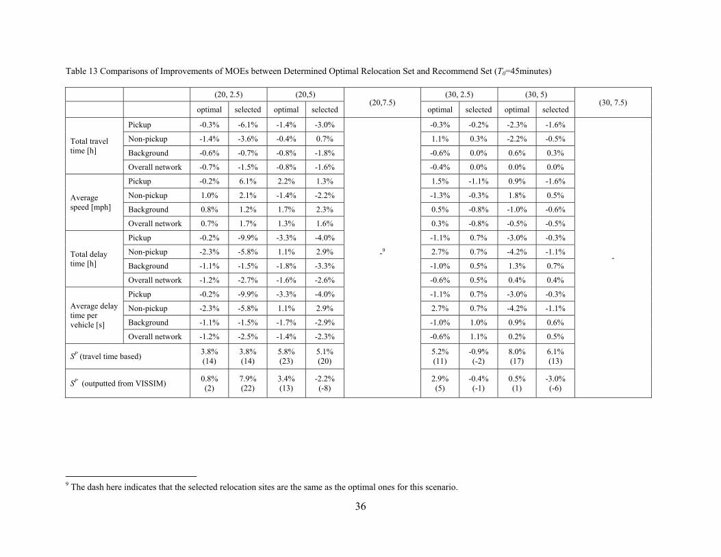
36


(20, 2.5) (20,5) (20,7.5)

(30, 2.5) (30, 5) (30, 7.5)

optimal selected optimal selected optimal selected optimal selected


Pickup -0.3% -6.1% -1.4% -3.0%

-9

-0.3% -0.2% -2.3% -1.6%

-

Non-pickup -1.4% -3.6% -0.4% 0.7% 1.1% 0.3% -2.2% -0.5%

Background -0.6% -0.7% -0.8% -1.8% -0.6% 0.0% 0.6% 0.3%

Overall network -0.7% -1.5% -0.8% -1.6% -0.4% 0.0% 0.0% 0.0%

Average speed [mph]

Pickup -0.2% 6.1% 2.2% 1.3% 1.5% -1.1% 0.9% -1.6%

Non-pickup 1.0% 2.1% -1.4% -2.2% -1.3% -0.3% 1.8% 0.5%

Background 0.8% 1.2% 1.7% 2.3% 0.5% -0.8% -1.0% -0.6%

Overall network 0.7% 1.7% 1.3% 1.6% 0.3% -0.8% -0.5% -0.5%


Pickup -0.2% -9.9% -3.3% -4.0% -1.1% 0.7% -3.0% -0.3%

Non-pickup -2.3% -5.8% 1.1% 2.9% 2.7% 0.7% -4.2% -1.1%

Background -1.1% -1.5% -1.8% -3.3% -1.0% 0.5% 1.3% 0.7%

Overall network -1.2% -2.7% -1.6% -2.6% -0.6% 0.5% 0.4% 0.4%

Average delay time per vehicle [s]

Pickup -0.2% -9.9% -3.3% -4.0% -1.1% 0.7% -3.0% -0.3%

Non-pickup -2.3% -5.8% 1.1% 2.9% 2.7% 0.7% -4.2% -1.1%

Background -1.1% -1.5% -1.7% -2.9% -1.0% 1.0% 0.9% 0.6%

Overall network -1.2% -2.5% -1.4% -2.3% -0.6% 1.1% 0.2% 0.5%

SP (travel time based) 3.8% (14)

3.8% (14)

5.8% (23)

5.1% (20)

5.2% (11)

-0.9% (-2)

8.0% (17)

6.1% (13)

SP (outputted from VISSIM) 0.8% (2)

7.9% (22)

3.4% (13)

-2.2% (-8)

2.9% (5)

-0.4% (-1)

0.5% (1)

-3.0% (-6)

9 The dash here indicates that the selected relocation sites are the same as the optimal ones for this scenario.

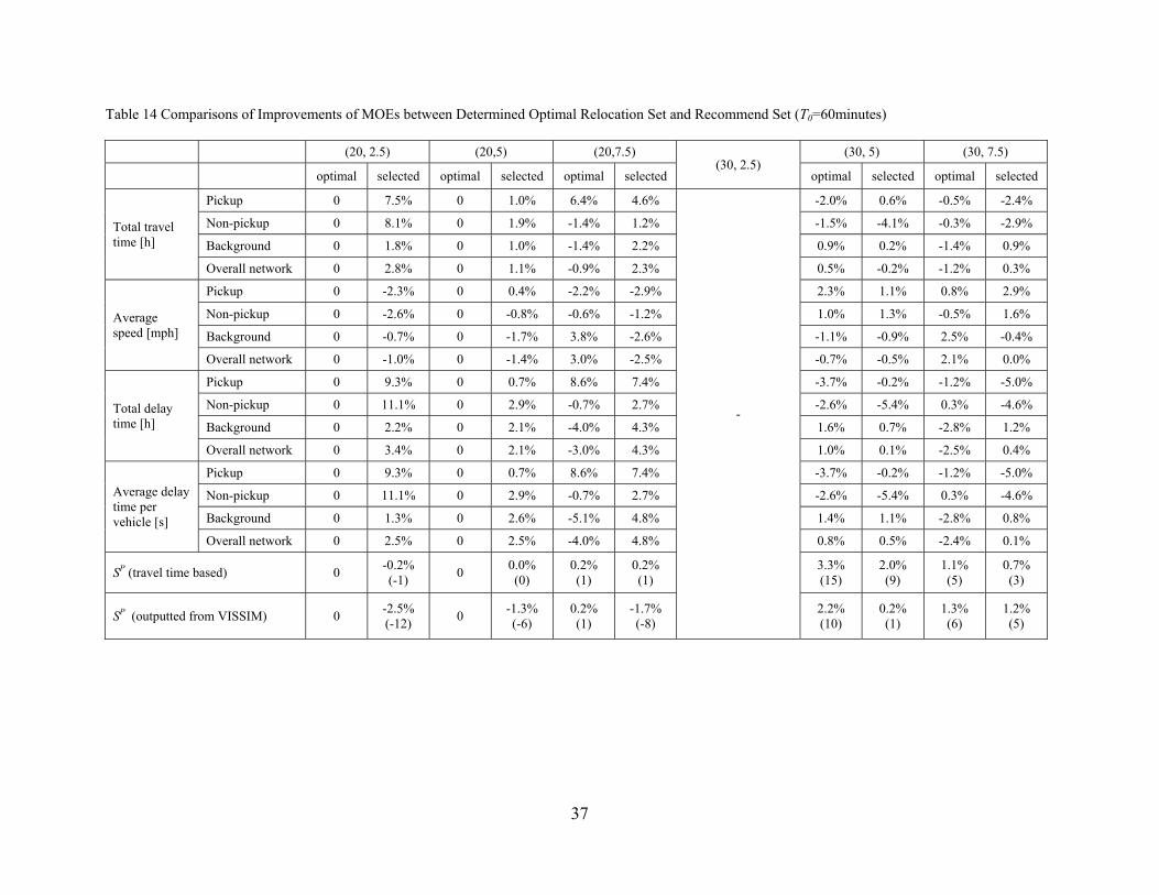
37


(20, 2.5) (20,5) (20,7.5) (30, 2.5)

(30, 5) (30, 7.5)

optimal selected optimal selected optimal selected optimal selected optimal selected


Pickup 0 7.5% 0 1.0% 6.4% 4.6%

-

-2.0% 0.6% -0.5% -2.4%

Non-pickup 0 8.1% 0 1.9% -1.4% 1.2% -1.5% -4.1% -0.3% -2.9%

Background 0 1.8% 0 1.0% -1.4% 2.2% 0.9% 0.2% -1.4% 0.9%

Overall network 0 2.8% 0 1.1% -0.9% 2.3% 0.5% -0.2% -1.2% 0.3%

Average speed [mph]

Pickup 0 -2.3% 0 0.4% -2.2% -2.9% 2.3% 1.1% 0.8% 2.9%

Non-pickup 0 -2.6% 0 -0.8% -0.6% -1.2% 1.0% 1.3% -0.5% 1.6%

Background 0 -0.7% 0 -1.7% 3.8% -2.6% -1.1% -0.9% 2.5% -0.4%

Overall network 0 -1.0% 0 -1.4% 3.0% -2.5% -0.7% -0.5% 2.1% 0.0%


Pickup 0 9.3% 0 0.7% 8.6% 7.4% -3.7% -0.2% -1.2% -5.0%

Non-pickup 0 11.1% 0 2.9% -0.7% 2.7% -2.6% -5.4% 0.3% -4.6%

Background 0 2.2% 0 2.1% -4.0% 4.3% 1.6% 0.7% -2.8% 1.2%

Overall network 0 3.4% 0 2.1% -3.0% 4.3% 1.0% 0.1% -2.5% 0.4%

Average delay time per vehicle [s]

Pickup 0 9.3% 0 0.7% 8.6% 7.4% -3.7% -0.2% -1.2% -5.0%

Non-pickup 0 11.1% 0 2.9% -0.7% 2.7% -2.6% -5.4% 0.3% -4.6%

Background 0 1.3% 0 2.6% -5.1% 4.8% 1.4% 1.1% -2.8% 0.8%

Overall network 0 2.5% 0 2.5% -4.0% 4.8% 0.8% 0.5% -2.4% 0.1%

SP (travel time based) 0 -0.2% (-1)

0 0.0% (0)

0.2% (1)

0.2% (1)

3.3% (15)

2.0% (9)

1.1% (5)

0.7% (3)

SP (outputted from VISSIM) 0 -2.5% (-12)

0 -1.3% (-6)

0.2% (1)

-1.7% (-8)

2.2% (10)

0.2% (1)

1.3% (6)

1.2% (5)

38

Chapter 5 Summary and Conclusions

This study developed a mathematical model to determine optimal sites where facilities move their dependents for pickup in a no-notice evacuation; the objective was to maximize successful evacuation of these dependents within a safe time threshold. The model was established based on anticipated travel time from the simulation model (VISSIM in this study), thus the two models interact with each other. In order to deal with the interaction, iteration between the two models was performed and a procedure to accomplish the iteration was proposed. The whole methodology was applied to a case study located in Chicago Heights, Illinois. The case study involved three facilities with 492 dependents and three safe time thresholds (i.e., 30, 45 and 60 minutes), introduced improvements of MOEs (e.g., total travel time, average speed, total delay time and average delay time per vehicle) and increases of SP (number of successful pickup evacuees) to evaluate performance of a relocation strategy, and tested sensitivity of the strategy to several factors (e.g., parents’ arrival time, number of dependents, and safe time). Finally, relocation sites were recommended based on the results of all scenarios.

In this study, the whole evacuation time period was discretized into several time intervals to reflect the fact that road traffic changes over time under no-notice evacuation. Travel time at each time interval was an input to the optimization model, playing a dominant role in determining optimal sites. In this study, simulated travel time, obtained from VISSIM, was used in the optimization model. As the precision of the simulated travel time could determine the success of the model, to examine if simulated travel time was reliable, we compared SP, directly output from VISSIM with SP calculated based on simulated travel time, found that the difference between them is in an acceptable scope and therefore believed that the optimization model is reliable.

Time that pickup evacuees arrive at the network was assumed to follow a Normal distribution in this study. Six arrival time distributions with different combinations of mean and standard deviation were tested for each safe time threshold, T0. The results showed that in most cases higher standard deviation or lower mean caused better network performance improvements by relocating facility dependents. Besides, an increase of SP was crucial to evaluate the effectiveness of the relocation strategy. From the perspective of increases of SP, a moderate range of T0 existed, so that if T0 fell into this range, an increase of successful pickup evacuees after relocation could be extensive. In this case study, T0=45 minutes was more likely in this range than T0=30 and 60 minutes. Improvements of MOEs and increases of SP were not necessarily consistent with each other - a relocation that leads to significant improvements for the network traffic performance does not necessarily cause significant increases of SP.

Optimal sets of relocation sites were diverse over scenarios. For the purpose of practical application, we generalized the results and presented the recommended optimal set(s). As T0 affected optimal sets of relocation sites, we here recommended relocation sites for each T0 individually. The results showed that in most cases, the recommended relocation sites gained more SP than the current sites, but the increase of SP was lower than the determined optimal sites to a relatively moderate extent. The recommended sites did not show a clear inclination to improve or deteriorate network performance, compared with the optimal ones.

In order to examine the influence of scale of pickup demand on performance of the relocation strategy, the total pickup demand was increased by 50% and tested with two arrival time distribution scenarios. The results showed that when pickup evacuees increase, both improvements of corresponding traffic performance and increases of SP are significantly magnified. That 106 more families (out of total 739 families) can successfully evacuate from the dangerous zone due to the proposed strategy is a striking contribution to evacuation management. However, these extraordinary improvements do not occur when T0 is fairly low (e.g., T0 = 30 minutes in this case study), and it should be noted that improvements of overall network performance maintain a slight extent and are not affected by

39

increasing the total number of pickup evacuees. To summarize, the main finding of exploring the sensitivity analysis to total number of pickup evacuees was that the relocation strategy is prominently effective if the safe evacuation time is adequate, as well as the amount of pickup evacuees. For the original pickup demand, only slight network performance improvements were found after implementing the relocation strategy, not exceeding 5%; however, with the previously mentioned finding, we could envision that when the facility relocation strategy is applied to a bigger scope that includes more facilities with more dependents, significant improvements of network performance and increases of successful pickup evacuees will be achieved by the relocation strategy. Furthermore, increasing pickup evacuees led to different inclinations to optimal sites; physical configuration of alternatives and their surrounding road network were found to affect determining optimal sites, and advantages of alternative sites with multiple entrances/exits showed up when a large amount of evacuees with pickup needs were involved.

This work was able to facilitate no-notice evacuation. Application of the proposed methodology to a certain area could assist local decision-makers to take effective measures during no-notice evacuation; the results could be part of local evacuation management plan.

The work had some limitations and allows more investigation in the future. First, the optimization model presented in this study is deterministic; in order to handle the randomness of the micro-simulation model, stochastic optimization methods could be introduced in the future to incorporate probabilistic elements. This study predetermined pickup evacuees’ origins and destinations outside the presented methodology; however, relocating dependents could lead to different destination choices (or even network arrival points). In the future, the relocation optimization program could integrate with a destination choice model. Additionally, in this study, only the auto mode was considered and only a small portion of facilities were involved. In the future, more facilities and more transportation modes will be conducted.

40

References

Chicago Heights School District 170. (2009). “Illinois School Report Card 2008.” < http://www.sd170.com> (March 1, 2009). Chiu, Y. C., Zheng, H., Villalobos, J., and Gautam, B. (2007). “Modeling no-notice mass evacuation using a dynamic traffic flow optimization model”, IIE Transactions, 39(1), 83-94. Church, R. L., and Cova, T. J. (2000). “Mapping evacuation risk on transportation networks using a spatial optimization model.” Transportation Research Part C: Emerging Technologies, 8(1), 321-336. Church, R. L., and Sexton, R. M. (2002). “Modeling small area evacuation: Can existing transportation infrastructure impede public safety?” <http://www.ncgia.ucsb.edu/vital/research/pubs/200204-Evacuation.pdf> (Oct. 23, 2008). Cova, T. J., and Church, R. L. (1997). “Modeling community evacuation vulnerability using GIS.” International Journal of Geographical Information Science, 11(8), 763-784. Cova, T. J., and Johnson, J. P. (2002). “Microsimulation of neighborhood evacuations in the urban-wildland interface.” Environment and Planning A, 34(12), 2211-29. Han, A. F. (1990). “TEVACS, decision support system for evacuation planning in Taiwan.” Journal of Transportation Engineering, 116(6), 821-830. Hobeika, A. G., and Kim, C. (1998). “Comparison of traffic assignments in evacuation modeling,” IEEE Transactions on Engineering Management, 45(2), 192-198. Hobeika, A.G., and Jamei, B. (1985). “MASSVAC: a model for calculating evacuation times under natural disasters.” Emergency Planning, Simulations Series 15, 23-28. Johnson, N. R. (1988). “Fire in a Crowded Theater: A Descriptive Investigation of the Emergence of Panic.” International Journal of Mass Emergencies and Disasters, 6(1), 7–26. KLD Associates. (1984). “Formulations of the DYNEV and I-DYNEV traffic simulation models used in ESF.” Federal Emergency Management Agency, Washington, D.C. Kongsomsaksakul, S., and Yang, C. (2005). “Shelter location-allocation model for flood evacuation planning.” Journal of the Eastern Asia Society for Transportation Studies, 6, 4237-4252. Lammel, G., Rieser, M., Nagel, K., Taubenbock, H., Strunz, G., Goseberg, N., Schlurmann, T., Klupfel, H., Setiadi, N., and Birkmann, J. (2008). “Emergency preparedness in the case of a Tsunami – Evacuation analysis and traffic optimization for the Indonesian city of Padang.” In Pedestrian and Evacuation Dynamics, Proceedings of the 4th international conference, Wuppertal. Lindell, M. K. (2008). “EMBLEM2: An empirically based large scale evacuation time estimate model.” Transportation Research Part A: Policy and Practice, 42(1), 140-154. Mei B. (2002). “Development of Trip Generation Models of Hurricane Evacuation.” Master Thesis, Louisiana State University. Murray-Tuite, P., and Mahmassani, H. S. (2003). “Model of household trip-chain sequencing in an emergency evacuation.” Transportation Research Record, 1831, 21–29. Murray-Tuite, P., and Mahmassani, H. S. (2004). “Transportation network evacuation planning with household activity interactions.” Transportation Research Record, 1894, 150-159.

41

Office of the Superintendent, Arlington High School. (2006). “Arlington Public Schools Important Information about Safety.” Massachusetts. <http://www.arlington.k12.ma.us/administration/schoolsafety/safetyltr10-17-06.pdf> (March 1, 2009). Owen, S.H., and Daskin, M.S. (1998). “Strategic facility location: a review.” European Journal of Operational Research, 111(3), 423-447. Pearce, V. (2008). “ITS to the Rescue.” US Department of Transportation, <http://www.its.dot.gov/eto/eto_rescue.htm> (Oct.23, 2008). PTV AG., (2005) VISSIM4.10 user manual. Sayyady, F. (2007). “Optimizing the use of public transit system in no-notice evacuations in urban areas.” Master Thesis, Mississippi State University. Sheffi Y. (1982). “A Note on Computer Graphics in Network Evacuation Studies.” IEEE Computer Graphics and Applications, 2(7), 57-62. Sheffi, Y., Mahmassani, H., and Powell, W. (1982). “A Transportation Network Evacuation Model.” Transportation Research Part A, 16(3), 209-218. Sherali, H. D., Carter, T. B., and Hobeika, A. G. (1991). “A Location-Allocation Model and Algorithm for Evacuation Planning Under Hurricane Flood Conditions,” Transportation Research B, 25(6), 439-452. Sime, J. D. (1995). “Crowd Psychology and Engineering.” Safety Science, 21(1), 1-14. Sinuany-Stern, Z., and Stern, E. (1993). “Simulating the Evacuation of a Small City: The Effects of Traffic Factors.” Socio-Economic Planning Sciences, 27(2), 97–108. Southworth, F. (1991). “Regional Evacuation Modeling: A State-of-the-Art Review.” Oak Ridge National Laboratory, Oak Ridge, TN. U.S. Census Bureau. (2000). “Census 2000.” <http://www.census.gov/main/www/cen2000.html> (March 1, 2009). U.S. Census Bureau. (2003). “Selected Statistics from the 2002 Economic Census.” <http://www.census.gov/econ/census02/ > (March 1, 2009). U.S. Census Bureau. (2008). “2005-2007 American Community Survey 3-Year Estimates.” <http://factfinder.census.gov/servlet/DatasetMainPageServlet?_program=ACS> (March 1, 2009). U.S. Census Bureau. (2009). “2008 Population Estimates.” <http://factfinder.census.gov/servlet/DatasetMainPageServlet?_program=PEP> (March 1, 2009). U.S. Department of Transportation (U.S. DOT), and U.S. Department of Homeland Security (U. S. DHS). (2006). “Report to Congress on Catastrophic Hurricane Evacuation Plan Evaluation.” <http://www.fhwa.dot.gov/reports/hurricanevacuation/rtc_chep_eval.pdf> (Oct.23, 2008). Yazici, M. A., and Ozbay, K. (2007). “Impact of probabilistic road capacity constraints on the spatial distribution of hurricane evacuation shelter capacities.” Transportation Research Record, 2022, 55-62. Zimmerman, C., Brodesky, R., and Karp, J. (2007). “Using Highways for No-Notice Evacuations: Routes to Effective Evacuation Planning Primer Series.” Technical Report.

FACILITATING NO-NOTICE EVACUATION … NO-NOTICE EVACUATION THROUGH OPTIMAL PICK-UP LOCATION...

Documents

Transcript of FACILITATING NO-NOTICE EVACUATION … NO-NOTICE EVACUATION THROUGH OPTIMAL PICK-UP LOCATION...