FACIAL EMOTION DETECTION USING CONVOLUTIONAL NEURAL NETWORKS

FACIAL EMOTION DETECTION USING CONVOLUTIONAL NEURAL

NETWORKS

by

Mohammed Adnan Adil

Bachelor of Engineering, Osmania University, 2016

A Report Submitted in Partial Fulfillment of the

Requirements for the Degree of

MASTER OF ENGINEERING

in the Department of Electrical and Computer Engineering

©Mohammed Adnan Adil, 2021

University of Victoria

All rights reserved. This report may not be reproduced in whole or in part, by photocopy or other means,

without the permission of the author.

i

SUPERVISORY COMMITTEE

Dr. T. Aaron Gulliver, Supervisor

(Department of Electrical and Computer Engineering)

Dr. Mihai Sima, Departmental Member

(Department of Electrical and Computer Engineering)

ii

ABSTRACT

Human emotions are the mental state of feelings and are spontaneous. There is no clear

connection between emotions and facial expressions and there is significant variability making

facial recognition a challenging research area. Features like Histogram of Oriented Gradient

(HOG) and Scale Invariant Feature Transform (SIFT) have been considered for pattern

recognition. These features are extracted from images according to manual predefined

algorithms. In recent years, Machine Learning (ML) and Neural Networks (NNs) have been used

for emotion recognition. In this report, a Convolutional Neural Network (CNN) is used to extract

features from images to detect emotions. The Python Dlib toolkit is used to identify and extract

64 important landmarks on a face. A CNN model is trained with grayscale images from the FER

2013 dataset to classify expressions into five emotions, namely happy, sad, neutral, fear and

angry. To improve the accuracy and avoid overfitting of the model, batch normalization and

dropout are used. The best model parameters are determined considering the training results.

The test results obtained show that CNN Model 1 is 80% accurate for four emotions (happy,

sad, angry, fear) and 72% accurate for five emotions (happy, sad, angry, neutral, fear), while

CNN Model 2 is 79% accurate for four emotions and 72% accurate for five emotions.

iii

CONTENTS

Supervisory Committee i

Abstract ii

List of Figures v

List of Tables vi

Abbreviations vii

Acknowledgement viii

Dedication ix

1. Introduction 1

1.1 Motivation 1

1.2 Facial emotion recognition 2

1.3 Literature review 4

1.4 Report structure 5

2. Dataset Preparation 6

2.1 Python libraries used 7

2.2 Image to arrays 8

2.3 Image to landmarks 9

3. Convolutional Neural Networks (CNN) 10

3.1 The CNN concept 11

3.1.1 Convolution operation 12

3.1.2 Pooling operation 13

3.1.3 Fully connected layer 14

3.1.4 Dropout 14

3.1.5 Batch normalization 14

3.1.6 Activation functions 15

iv

3.2 CNN architecture 16

3.3 Compiling the model 20

3.4 Training the model 20

4. Results and discussion 21

4.1 Evaluation parameters 21

4.2 Determining the best parameter values for models 1 and 2 23

4.3 CNN Model 1 results 28

4.4 CNN Model 2 results 29

4.5 Comparison and evaluation of results 31

4.6 Comparison of results with other emotion recognition models 33

5. Conclusion 34

5.1 Future work 35

Bibliography 36

v

LIST OF FIGURES

Figure 1.1 FER procedure for an image [9]. 2

Figure 1.2 Facial landmarks to be extracted from a face. 2

Figure 2.1 OneHot encoding example. 8

Figure 2.2 Sad image from the FER 2013 dataset converted into an array. 8

Figure 2.3 Attributes of a sad image. 9

Figure 2.4 Landmarks detected on a face. 9

Figure 3.1 The basic structure of a neuron [31]. 10

Figure 3.2 A multi output NN with two neurons [31]. 11

Figure 3.3 A fully connected NN [31]. 11

Figure 3.4 The CNN operations [33]. 12

Figure 3.5 Convolving a 5 × 5 image with a 3 × 3 kernel to get a 3 × 3 convolved feature [33]. 13

Figure 3.6 Max and average pooling outputs for an image [33]. 13

Figure 3.7 Dropout in a NN. 14

Figure 3.8 The location of the softmax function [31]. 15

Figure 3.9 Structure of a CNN. 16

Figure 3.10 Architecture of CNN Model 1 with the input and output attributes. 18

Figure 3.11 Architecture of CNN Model 2 with the input and output attributes. 19

Figure 4.1 Confusion matrix for five emotions. 22

Figure 4.2 Results after training CNN Model 1 for 100 epochs (a) accuracy and (b) loss. 24

Figure 4.3 Results after training CNN Model 1 for 400 epochs (a) accuracy and (b) loss. 24

vi

LIST OF TABLES

Table 1.1 Definitions of 64 primary and secondary landmarks. 3

Table 1.2 A summary of FER systems based on DL. 4

Table 3.1 Convolution parameters selected. 17

Table 3.2 The number of parameters in CNN models 1 and 2. 19

Table 4.1 The parameter values considered. 23

Table 4.2 The image data preprocessing methods considered. 23

Table 4.3 Early stopping parameters and their functions. 25

Table 4.4 Early stopping values chosen for the two models. 25

Table 4.5 Parameter values for Cases 1 to 5 with CNN Model 1. 26

Table 4.6 Results for Cases 1 to 5 with CNN Model 1. 26





Table 4.11 Performance of CNN Model 1 with five emotions. 28

Table 4.12 Performance of CNN Model 1 with four emotions. 29

Table 4.13 Performance of CNN Model 2 with five emotions. 30

Table 4.14 Performance of CNN Model 2 with four emotions. 30

Table 4.15 Performance of CNN models 1 and 2 with five emotions. 32

Table 4.16 Performance of CNN models 1 and 2 with four emotions. 32

Table 4.17 DL based emotion recognition approaches and their accuracy. 33

vii

ABBREVATIONS

HOG Histogram of Oriented Gradient

SIFT Scale Invariant Feature Transform

ML Machine Learning

NN Neural Network

CNN Convolutional Neural Network

FER 2013 Facial Emotion Recognition 2013 Dataset

FER Facial Emotion Recognition

AI Artificial Intelligence

DL Deep Learning

EEG Electroencephalograph

HCI Human Computer Interaction

FE Feature Extraction

CV Computer Vision

RNN Recurrent Neural Network

MMOD Maximum Margin Object Detection

NumPy Numerical Python

ELU Exponential Linear Unit

API Application Programming Interface

TP True Positive

FP False Positive

FN False Negative

TN True Negative

ANN Artificial Neural Network

LR Learning Rate

RNN Recurrent Neural Network

viii

ACKNOWLEDGEMENT

I would like to thank Almighty Allah for giving me confidence and the ability to pursue a Master

of Engineering degree. I am happy that my educational journey has been a fantastic experience

with a lot of learning curves.

I would like to thank my supervisor Dr. T. Aaron Gulliver for being super cool and an amazing

mentor. He always helped me when I needed him and I had no trouble studying under his

guidance. He motivated me whenever needed and helped me choose courses, even when I

wanted to do a course outside the Department of Electrical and Computer Engineering. He was

supportive throughout the whole program, always responded to my emails, even meeting

around 11 pm to help out with academic support. I am fortunate to have had amazing

professors like Dr. Mihai Sima, Dr. Issa Traore and Dr. Gary Perkins with immense knowledge

and great passion towards the courses they teach. I thank the staff of the University of Victoria

who contributed in many ways to the successful completion my degree.

ix

DEDICATION

To my girlfriend for her support and trust in my abilities.

1

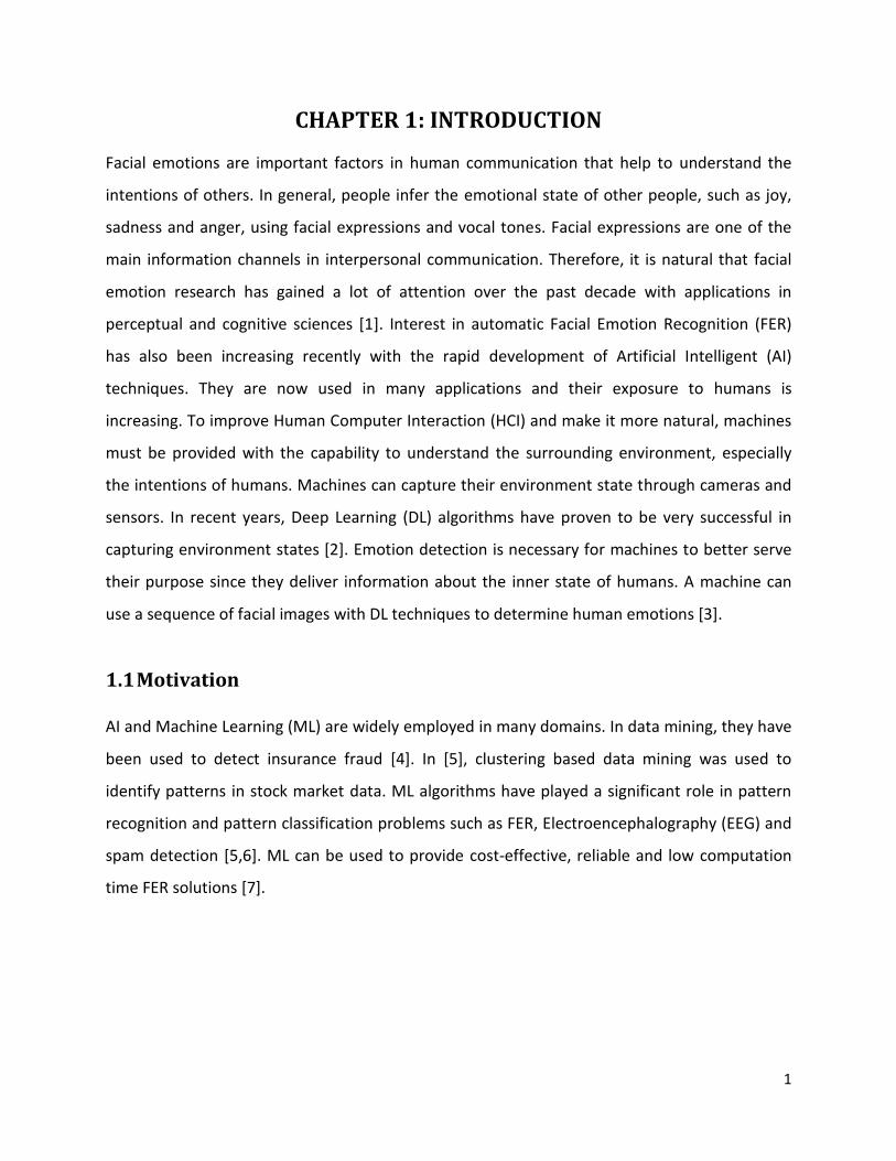
CHAPTER 1: INTRODUCTION

Facial emotions are important factors in human communication that help to understand the

intentions of others. In general, people infer the emotional state of other people, such as joy,

sadness and anger, using facial expressions and vocal tones. Facial expressions are one of the

main information channels in interpersonal communication. Therefore, it is natural that facial

emotion research has gained a lot of attention over the past decade with applications in

perceptual and cognitive sciences [1]. Interest in automatic Facial Emotion Recognition (FER)

has also been increasing recently with the rapid development of Artificial Intelligent (AI)

techniques. They are now used in many applications and their exposure to humans is

increasing. To improve Human Computer Interaction (HCI) and make it more natural, machines

must be provided with the capability to understand the surrounding environment, especially

the intentions of humans. Machines can capture their environment state through cameras and

sensors. In recent years, Deep Learning (DL) algorithms have proven to be very successful in

capturing environment states [2]. Emotion detection is necessary for machines to better serve

their purpose since they deliver information about the inner state of humans. A machine can

use a sequence of facial images with DL techniques to determine human emotions [3].

1.1 Motivation

AI and Machine Learning (ML) are widely employed in many domains. In data mining, they have

been used to detect insurance fraud [4]. In [5], clustering based data mining was used to

identify patterns in stock market data. ML algorithms have played a significant role in pattern

recognition and pattern classification problems such as FER, Electroencephalography (EEG) and

spam detection [5,6]. ML can be used to provide cost-effective, reliable and low computation

time FER solutions [7].

2

1.2 Facial emotion recognition

FER typically has four steps. The first is to detect a face in an image and draw a rectangle

around it and the next step is to detect landmarks in this face region. The third step is

extracting spatial and temporal features from the facial components. The final step is to use a

Feature Extraction (FE) classifier and produce the recognition results using the extracted

features. Figure 1.1 shows the FER procedure for an input image where a face region and facial

landmarks are detected. Facial landmarks are visually salient points such as the end of a nose,

and the ends of eyebrows and the mouth as shown in Figure 1.2. The pairwise positions of two

landmark points or the local texture of a landmark are used as features. Table 1.1 gives the

definitions of 64 primary and secondary landmarks [8]. The spatial and temporal features are

extracted from the face and the expression is determined based on one of the facial categories

using pattern classifiers.

Figure 1.1 FER procedure for an image [9].

Figure 1.2 Facial landmarks to be extracted from a face.

3

Primary landmarks Secondary landmarks

Number Definition Number Definition

16 Left eyebrow outer corner 1 Left temple

19 Left eyebrow inner corner 8 Chin tip

22 Right eyebrow inner corner 2-7,9-14 Cheek contours

25 Right eyebrow outer corner 15 Right temple

28 Left eye outer corner 16-19 Left eyebrow contours

30 Left eye inner corner 22-25 Right eyebrow corners

32 Right eye inner corner 29,33 Upper eyelid centers

34 Right eye outer corner 31,35 Lower eyelid centers

41 Nose tip 36,37 Nose saddles

46 Left mouth corner 40,42 Nose peaks (nostrils)

52 Right mouth corner 38-40,42-45 Nose contours

63,64 Eye centers 47-51,53-62 Mouth contours

Table 1.1 Definitions of 64 primary and secondary landmarks.

DL based FER approaches greatly reduce the dependence on face-physics based models and

other preprocessing techniques by enabling end to end learning directly from the input images

[10]. Among DL models, Convolutional Neural Networks (CNNs) are the most popular. With a

CNN, an input image is filtered through convolution layers to produce a feature map. This map

is then input to fully connected layers, and the facial expression is recognized as belonging to a

class based on the output of the FE classifier.

The dataset used for this model is the Facial Emotion Recognition 2013 (FER 2013) dataset [11].

This is an open source dataset that was created for a project then shared publicly for a Kaggle

competition. It consists of 35,000 grayscale size 48 × 48 face images with various emotion

labels. For this project, five emotions are used, namely happy, angry, neutral, sad and fear.

4

1.3 Literature review

Facial expressions are used by humans to convey mood. Automatic facial expression analysis

tools [12] have applications in robotics, medicine, driving assist systems, and lie detection

[13,14,15]. Recent advances in FER [16] have led to improvements in neuroscience [17] and

cognitive science [18]. Further developments in Computer Vision (CV) [19], and ML [20] have

made emotion identification more accurate and accessible. Table 1.2 gives a summary of FER

systems based on DL methods.

Reference Emotions analyzed Recognition algorithm Database

Hybrid CNN-RNN [21] Seven emotions

(angry, disgust, fear, happy,

sad, surprise, neutral)

1. Hybrid Recurrent Neural Network (RNN)-CNN framework for propagating information over a sequence 2. Temporal averaging is used for aggregation

EmotiW [26]

Spatio temporal feature

representation [22]

Six emotions


sad, surprise)

1. Spatial image characteristics of the representative expression state frames are learned using a CNN 2. Temporal characteristics of the spatial feature representation in the first part are learned using a long short term memory model

MMI [27]

CASME II [28]

Joint fine tuning [23]

Seven emotions


sad, surprise, neutral)

Two different models 1. CNN for temporal appearance features 2. CNN for temporal geometry features from temporal facial landmark points

CK+ [29]

MMI [31]

Candide-3 [24]

Six emotions (angry, disgust, fear, happy,

sad, surprise)

1. Candide-3 model in conjunction with a learned objective function for face model fitting 2. RNN for temporal dependencies present in the image sequences during classification

CK+ [29]

Multi angle FER [25]

Six emotions

(angry, disgust, fear, happy, sad, neutral)

1. Extraction of texture patterns and the relevant key features of the facial points 2. CNN to predict labels for the facial expressions

CK+ [29]

MMI [31]

Table 1.2 A summary of FER systems based on DL.

5

1.4 Report structure

The report structure is as follows.

Chapter 1 provided a brief overview of FER, the motivation for this work and the methodology

used in FER. The related work was also discussed.

Chapter 2 introduces the Python libraries used for preparing the dataset. The conversion of

images into arrays and extracting landmark features from images in the FER 2013 dataset is

explained in detail.

Chapter 3 provides an overview of CNNs and the model structure including the layers and their

functions. Training and compiling of the model is also explained.

Chapter 4 presents the results obtained using several metrics. The choice of model parameters

is explained and the results are compared with those of other networks. The performance of

two models is evaluated and discussed.

Chapter 5 concludes the report by providing a brief summary of the results and some topics for

future work.

6

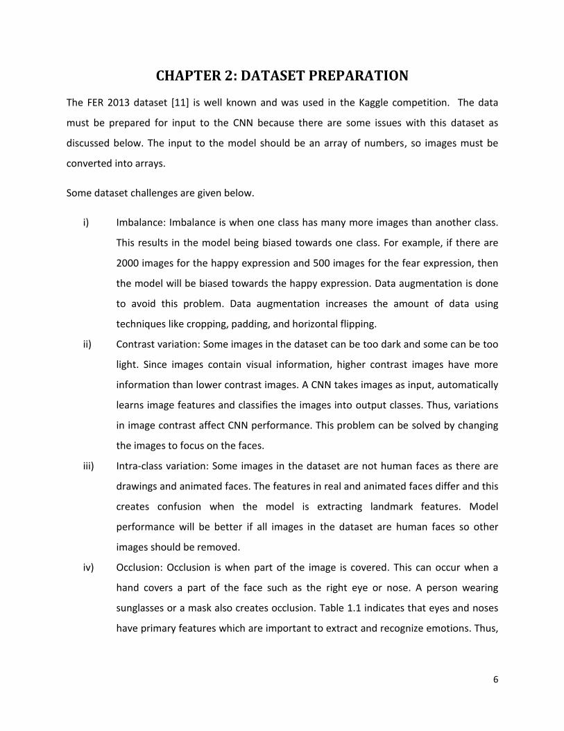
CHAPTER 2: DATASET PREPARATION

The FER 2013 dataset [11] is well known and was used in the Kaggle competition. The data

must be prepared for input to the CNN because there are some issues with this dataset as

discussed below. The input to the model should be an array of numbers, so images must be

converted into arrays.

Some dataset challenges are given below.

i) Imbalance: Imbalance is when one class has many more images than another class.

This results in the model being biased towards one class. For example, if there are

2000 images for the happy expression and 500 images for the fear expression, then

the model will be biased towards the happy expression. Data augmentation is done

to avoid this problem. Data augmentation increases the amount of data using

techniques like cropping, padding, and horizontal flipping.

ii) Contrast variation: Some images in the dataset can be too dark and some can be too

light. Since images contain visual information, higher contrast images have more

information than lower contrast images. A CNN takes images as input, automatically

learns image features and classifies the images into output classes. Thus, variations

in image contrast affect CNN performance. This problem can be solved by changing

the images to focus on the faces.

iii) Intra-class variation: Some images in the dataset are not human faces as there are

drawings and animated faces. The features in real and animated faces differ and this

creates confusion when the model is extracting landmark features. Model

performance will be better if all images in the dataset are human faces so other

images should be removed.

iv) Occlusion: Occlusion is when part of the image is covered. This can occur when a

hand covers a part of the face such as the right eye or nose. A person wearing

sunglasses or a mask also creates occlusion. Table 1.1 indicates that eyes and noses

have primary features which are important to extract and recognize emotions. Thus,

7

occluded images should be removed from the dataset as the model cannot

recognize emotions from these images.

The images used for training should be free from the above issues. Thus, manual filtering of

the 35,000 images in the FER 2013 dataset was done and 7,074 images from five classes

were selected, 966 for angry, 859 for fear, 2477 for happy, 1466 for neutral and 1326 for

sad.

2.1 Python libraries used

NumPy: Numerical Python (NumPy) is an open source Python library used for working with

arrays and matrices. An array object in NumPy is called nd.array. CNN inputs are arrays of

numbers and NumPy can be used to convert images into NumPy arrays to easily perform matrix

multiplications and other CNN operations.

OpenCV: OpenCV is an open source library for CV, ML and image processing. Images and videos

can be processed by OpenCV to identify objects, faces and handwriting. When it is integrated

with a library such as Numpy, OpenCV can process array structures for analysis. Mathematical

operations are performed on these array structures for pattern recognition.

Dlib: Dlib v19.2 uses a Maximum-Margin Object Detector (MMOD) with CNN based features.

Training with this library is simple and a large amount of data is not needed. After labeling

landmarks in an image, it learns to detect them. This also has an inbuilt shape and frontal face

detector.

OneHot encoder: This is part of the ML tool in Python called Scikit-learn. A common approach

to converting categories into a suitable format for input to a ML or DL model is OneHot

encoding. For example, consider the four employment categories student, teacher, doctor and

banker. A OneHot encoding is shown in Figure 2.1. In this figure, each category is represented

by a four-dimensional vector with one non zero entry which has a value of one.

8

Figure 2.1 OneHot encoding example.

Math: Common mathematical functions are defined in the math library. These include

trigonometric functions, representation functions, logarithmic functions and angle conversion

functions. CNN operations require adding and multiplying arrays which can be done using this

library.

Facealigner: It was shown in [30] that face alignment can improve the accuracy of FER models

by almost 1%. A face aligner forms a rectangle on the face and ensures all landmark features

are inside this rectangle. This also eliminates unwanted data in images.

The libraries mentioned above are either pre-installed or can be installed using the pip function

in Python. The functions in these libraries are used to prepare the data for input to a CNN.

2.2 Image to arrays

An image is represented by values (numbers) that correspond to the pixel intensities. The array

module in NumPy (nd.array) is used to convert an image into an array and obtain the image

attributes. Figure 2.2 shows an image in the sad class from the FER 2013 dataset converted into

a NumPy array. Figure 2.3 shows the attributes of this image which are 2304 pixels, 2

dimensions and size 48 × 48 pixels.

Figure 2.2 Sad image from the FER 2013 dataset converted into an array.

9

Figure 2.3 Attributes of a sad image.

2.3 Image to landmarks

The Dlib library is used to detect facial landmarks. This process consists of two steps, localize

the face in an image and detect the facial landmarks. The frontal face detector from Dlib is used

to detect the face in an image. A rectangle on the face is obtained which is defined by the top

left corner and the bottom right corner coordinates. The Dlib shape predictor is used to extract

the key facial features from an input image. An object called landmarks which has two

arguments is passed. The first argument is an image in which faces will be detected and the

second specifies the area where the facial landmarks will be obtained. This area is represented

by the coordinates of the rectangle. Figure 2.4 shows the 64 landmarks detected in an image.

Input image step(a) step(b)

Figure 2.4 Landmarks detected on a face.

10

CHAPTER 3: CONVOLUTIONAL NEURAL NETWORKS

The fundamental building block of a NN is a neuron. Figure 3.1 shows the structure of a neuron.

Forward propagation of information through a neuron happens when inputs to are

multiplied by their corresponding weights and then added together. This result is passed

through a nonlinear activation function along with a bias term which shifts the output. The bias

is shown as in Figure 3.1. For an input vector = , ,…, and weight vector = ,

,..., , the neuron output is ̂ = ∑ . The output is between 0 and 1 which

makes it suitable for problems with probabilities. The purpose of the activation function is to

introduce nonlinearities in the network since most real world data is nonlinear. The use of a

nonlinear function also allows NNs to approximate complex functions.

Figure 3.1 The basic structure of a neuron [31].

Neurons can be combined to create a multi output NN. If every input has a connection to every

neuron it is called dense or fully connected. Figure 3.2 shows a dense multi output NN with two

neurons. A deep NN has multiple hidden layers stacked on top of each other and every neuron

in each hidden layer is connected to a neuron in the previous layer. Figure 3.3 shows a fully

connected NN with 5 layers.

11

Figure 3.2 A multi output NN with two neurons [31].

Figure 3.3 A fully connected NN [31].

3.1 The CNN concept

A CNN is a DL algorithm which takes an input image, assigns importance (learnable weights and

biases) to various aspects/objects in the image and is able to differentiate between images. The

preprocessing required in a CNN is much lower than other classification algorithms. Figure 3.4

shows the CNN operations. The architecture of a CNN is analogous to that of the connectivity

pattern of neurons in the human brain and was inspired by the organization of the visual cortex

[32]. One role of a CNN is to reduce images into a form which is easier to process without losing

features that are critical for good prediction. This is important when designing an architecture

which is not only good at learning features but also is scalable to massive datasets. The main

12

CNN operations are convolution, pooling, batch normalization and dropout which are described

below.

Figure 3.4 The CNN operations [33].

3.1.1 Convolution operation

The objective of the convolution operation is to extract high level features such as edges from

an input image. The convolution layer functions are as follows.

The first convolutional layer(s) learns features such as edges, color, gradient orientation

and simple textures.

The next convolutional layer(s) learns features that are more complex textures and

patterns.

The last convolutional layer(s) learns features such as objects or parts of objects.

The element involved in carrying out the convolution operation is called the kernel. A kernel

filters everything that is not important for the feature map, only focusing on specific

information. The filter moves to the right with a certain stride length till it parses the complete

width. Then, it goes back to the left of the image with the same stride length and repeats the

process until the entire image is traversed.

Figure 3.5 presents an image with dimensions 5 × 5 (shown in green) and the following 3 × 3

kernel filter

13

The stride length is chosen as one so the kernel shifts nine times, each time performing a matrix

multiplication of the kernel and the portion of the image under it.

Figure 3.5 Convolving a 5 × 5 image with a 3 × 3 kernel to get a 3 × 3 convolved feature [33].

The convolved feature can have the same dimensions as the input or the kernel. This is done by

same or valid padding. Same padding is when the convolved feature has the dimensions of the

input image and valid padding is when this feature has the dimensions of the kernel.

3.1.2 Pooling operation

The pooling layer reduces the spatial size of a convolved feature. This is done to decrease the

computations required to process the data and extract dominant features which are rotation

and position invariant. There are two types of pooling, namely max pooling and average

pooling. Max pooling returns the maximum value from the portion of the image covered by the

kernel, while average pooling returns the average of the corresponding values. Figure 3.6 shows

the outputs obtained by performing max and average pooling on an image.

Figure 3.6 Max and average pooling outputs for an image [33].

14

3.1.3 Fully connected layer

Neurons in a fully connected layer have connections to all neurons in the previous layer. This

layer is found towards the end of a CNN. In this layer, the input from the previous layer is

flattened into a one-dimensional vector and an activation function is applied to obtain the

output.

3.1.4 Dropout

Dropout is used to avoid overfitting. Overfitting in an ML model happens when the training

accuracy is much greater than the testing accuracy. Dropout refers to ignoring neurons during

training so they are not considered during a particular forward or backward pass leaving a

reduced network. These neurons are chosen randomly and an example is shown in Figure 3.7.

The dropout rate is the probability of training a given node in a layer, where 1.0 means no

dropout and 0.0 means all outputs from the layer are ignored.

Figure 3.7 Dropout in a NN

3.1.5 Batch normalization

Training a network is more efficient when the distributions of the layer inputs are the same.

Variations in these distributions can make a model biased. Batch normalization is used to

normalize the inputs to the layers.

15

3.1.6 Activation functions

Softmax and Exponential Linear Unit (ELU) are activation functions commonly used in CNNs and

are described below. The softmax function is given by

∑

where the are the input values and is the number of input values. This function converts

real numbers into probabilities as it ensures the output values sum to 1 and are in the range 0

to 1. Softmax is used in the fully connected layer of the proposed models so the results can be

interpreted as a probability distribution for the five emotions. Figure 3.8 shows the location of

the softmax function.

Figure 3.8 The location of the softmax function [31].

The ELU function is

{ ,

,

16

where is the input value and α is the slope. This function saturates to a negative value when

is negative and α controls the saturation. This decreases the information passed to the next

layer [38].

3.2 CNN architecture

ML models can be built and trained easily using a high level Application Programming Interface

(API) like Keras. In this report, a sequential CNN model is developed using Tensorflow with the

Keras API since it allows a model to be built layer by layer. Tensorflow is an end to end open

source platform for ML. It has a flexible collection of tools, libraries and community resources

to build and deploy ML applications. Figure 3.9 shows the structure of a CNN where conv.

denotes convolution.

Figure 3.9 Structure of a CNN.

CNN Model 1 has four phases. At the end of each phase, the size of the input image is reduced.

The first three phases have the same layers where each starts with a convolution and ends with

dropout. The first phase of the model has an input layer for an image of size 48 × 48 (height

and width in pixels) and convolution is performed on this input. Table 3.1 shows the

convolution parameters which are the same for all convolution layers in the network except the

number of kernels. An He-normal initializer [39] is used which randomly generates appropriate

values for the kernel. The number of kernels is 64 in the first phase. Then, batch normalization

is performed to obtain the inputs to the next layer. Convolution and batch normalization are

repeated in the following layers. In the next layer, max pooling is performed with pool size 2 ×

2, so the output size is 24 × 24. Dropout is performed next at a rate of 0.35. The second phase

has 128 kernels and 0.4 dropout rate. Max pooling in the second phase gives an output of size

12 × 12. The third phase has 256 kernels with 0.5 dropout rate. Max pooling in the third phase

Input layer

Conv. layer

Batch normalize

Pooling Dropout Dense

17

reduces the size of the output to 6 × 6. The final phase starts with a flatten layer followed by

dense and output layers. Classifying the five emotions requires the data to be a one-

dimensional array. The flatten layer converts the two-dimensional data into a one-dimensional

array. The flattened output is fed to the dense layer which applies the softmax function. Then,

batch normalization is done and the output layer gives the class probabilities.

Kernel size

Padding Same

Activation ELU

Kernel initializer He-normal

Kernels 64, 128, 256

Table 3.1 The convolution parameters.

CNN Model 2 is similar to Model 1 but with some reduced layers. In CNN Model 1, the first

three phases have two convolution and batch normalization layers followed by pooling, but for

CNN Model 2 these phases have one convolution and batch normalization layer followed by

pooling. The rest of the Model 2 architecture is the same as Model 1. Figure 3.10 shows the

architecture of CNN Model 1 with the input and output attributes. Figure 3.11 shows the

architecture of CNN Model 2 with the input and output attributes. Table 3.2 gives the number

of trainable and non-trainable parameters in the two models.

18

Figure 3.10 Architecture of CNN Model 1 with the input and output attributes.

19

Figure 3.11 Architecture of CNN Model 2 with the input and output attributes.

CNN Model 1 CNN Model 2

Number of parameters 3,510,469 2,734,085

Trainable parameters 3,507,781 2,732,293

Non-trainable parameters 2,688 1,792

Table 3.2 The number of parameters in CNN models 1 and 2.

20

3.3 Compiling the model

Compiling the model requires two parameters, optimizer and metrics. The optimizers used are

Adam and Nadam. The optimizer is used to update the weights in a DL model based on the loss.

The metrics used are accuracy, categorical cross-entropy loss, precision, recall and F-score.

These metrics are defined in Chapter 4.

3.4 Training the model

To train the model, the train-test split() function is used. This function splits the dataset into

training and testing sets. The training data is not used for testing. A training ratio of 0.90 means

90% of the dataset will be used for training and the remaining for testing the model. The

Learning Rate (LR) is a configurable parameter used in training which determines how fast the

model weights are calculated. A high LR can cause the model to converge too quickly while a

small LR may lead to more accurate weights (up to convergence) but takes more computation

time. The number of epochs is the number of times a dataset is passed forward and backward

through the NN. The dataset is divided into batches to lower the processing time and the

number of training images in a batch is called the batch size.

21

CHAPTER 4: RESULTS AND DISCUSSION

In this chapter, the metrics used to evaluate model performance are defined. Then the best

parameter values for each model are determined from the training results. These values are

used to evaluate the accuracy and loss for CNN models 1 and 2. The results for these models

are then compared and discussed.

4.1 Evaluation metrics

Accuracy, loss, precision, recall and F-score are the metrics used to measure model

performance. These metrics are defined below.

Accuracy: Accuracy is given by

Accuracy =

Loss: Categorical cross-entropy is used as the loss function and is given by

Loss ∑ ( , , )

where y is a binary indicator (0 or 1), p is the predicted probability and m is the number of

classes (happy, sad, neutral, fear, angry)

Confusion matrix: The confusion matrix provides values for the four combinations of true and

predicted values, True Positive (TP), True Negative (TN), False Positive (FP) and False Negative

(FN). Precision, recall and F-score are calculated using TP, FP, TN, FN. TP is the correct

prediction of an emotion, FP is the incorrect prediction of an emotion, TN is the correct

prediction of an incorrect emotion and FN is the incorrect prediction of an incorrect emotion.

Consider an image from the happy class. The confusion matrix for this example is shown in

Figure 4.1. The red section has the TP value as the happy image is predicted to be happy. The

blue section has FP values as the image is predicted to be sad, angry, neutral or fear. The yellow

22

section has TN values as the image is not sad, angry, neutral or fear but the model predicted

this. The green section has FN values as the image is not happy but was predicted to be happy.

Recall: Recall is given by

Recall =

Precision: Precision is given by

Precision =

F-score: F-score is the harmonic mean of recall and precision and is given by

F-score =

23

4.2 Determining the best parameter values for models 1 and 2

The parameters LR, batch size, training ratio, number of epochs, image preprocessing method

and optimizer are determined in this section. Table 4.1 gives the parameter values considered

for these models. These values were chosen because they are commonly used in the literature.

The three image preprocessing methods considered are given in Table 4.2. After applying these

methods, 524 images were added to fear, 630 to angry and 224 to sad. Thus, the total number

of images was increased to 8,472 from 7,074 (1490 for angry, 1489 for fear, 2477 for happy,

1466 for neutral and 1550 for sad). The metric values given in the following tables are test

results.

Parameter Values

LR 0.1, 0.01, 0.001

Batch size 16, 32

Training ratio 0.85, 0.5, 0.25

Image preprocessing method Method 1, Method 2, Method 3

Optimizer Adam, Nadam

Table 4.1 The parameter values considered.

Parameter Method 1 Method 2 Method 3

Rotation range (0-180o) 10 8 5

Width shift range (fraction of width of an image) 0.10 0.08 0.05

Height shift range (fraction of height of an image) 0.10 0.08 0.05

Shear range (Image distorted along the axes) 0.10 0.20 0.30

Zoom range (0-1) 0.10 0.08 0.08

Horizontal flip True True True

Table 4.2 The image preprocessing methods considered.

Model 1 was trained with the parameter values LR = 0.01, batch size = 16, training ratio = 0.8,

epochs = 100 and Adam optimizer. Figure 4.1 shows the results of one trial after training the

model for 100 epochs. Over fifty trials, the accuracy varied between 0.68 and 0.72. The model

was then trained for 400 epochs and Figure 4.2 shows the results of one trial. Over five trials,

24

the accuracy was still between 0.68 and 0.72. These results show that training with more

epochs increased the loss and computation time. Early stopping in Keras was used to stop

training once the model performance converges. Table 4.3 gives the early stopping parameters

and their functions. The value of min_delta was chosen as 0.0001 as higher values resulted in

lower accuracy. Results for 55 trials showed that once the accuracy reaches 0.72, it stops

improving. Typically, an improvement in accuracy occurs over a span of 20 epochs. Thus, the

early stopping parameter values given in Table 4.4 were chosen.

Figure 4.2 Results of one trial after training Model 1 for 100 epochs (a) accuracy and (b) loss.

Figure 4.3 Results of one trial after training Model 1 for 400 epochs (a) accuracy and (b) loss.

25

Parameter Function

Monitor Metric to be monitored

Min_delta Minimum change in the monitored metric to qualify as an improvement, i.e. a

change of less than min_delta, will count as no improvement

Patience Number of epochs with no improvement after which training will be stopped

Restore best

weights

Whether to restore model weights with the best value of the monitored

metric. If false, the model weights obtained at the last step of training are

used.

Table 4.3 Early stopping parameters and their functions.

Parameter Value

Monitor Accuracy

Min_delta 0.0001

Patience 25 epochs

Restore best weights True

Table 4.4 Early stopping values chosen for the two models.

The best LR, batch size, training ratio, image preprocessing method and optimizer are now

determined for CNN Model 1. The values considered for Cases 1 to 5 are shown in Table 4.5 and

Table 4.6 shows the corresponding results. In Table 4.6, Acc denotes accuracy and Avg denotes

average. Four trials were conducted for each case and the highest average accuracy of 0.72

with minimum average loss 0.90 was obtained in Case 2. Cases 6 to 9 considered the training

ratios and image preprocessing methods in Table 4.7, and the corresponding results are given in

Table 4.8. Case 2 still has the highest average accuracy of 0.72 with minimum average loss 0.90.

Based on the results for Cases 1 to 9, the best parameter values for CNN Model 1 are LR = 0.01,

batch size = 16, training ratio = 0.85, Adam optimizer and image preprocessing Method 1.

26

Table 4.5 Parameter values for Cases 1 to 5 with CNN Model 1.

Case 1 Case 2 Case 3 Case 4 Case 5

Trial Acc Loss Acc Loss Acc Loss Acc Loss Acc Loss

1 0.22 1.84 0.71 0.90 0.65 1.24 73.28 0.89 0.72 0.78

2 0.25 1.73 0.72 0.88 0.66 1.51 71.21 0.96 0.70 0.81

3 0.25 2.02 0.72 1.04 0.66 1.28 71.33 0.90 0.69 0.88

4 0.24 2.10 0.72 0.89 0.64 1.31 72.06 0.93 0.66 1.32

Avg 0.24 1.90 0.72 0.90 0.65 1.33 0.71 0.92 0.69 0.94

Table 4.6 Results for Cases 1 to 5 with CNN Model 1.

Table 4.7 Parameter values for Cases 6 to 9 with CNN Model 1.

Case 6 Case 7 Case 8 Case 9

Trial Acc Loss Acc Loss Acc Loss Acc Loss

1 0.71 0.86 0.69 0.93 0.67 1.14 0.60 1.12

2 0.70 0.89 0.69 0.98 0.65 1.19 0.63 1.08

3 0.71 0.78 0.68 1.04 0.69 1.06 0.61 1.24

4 0.69 0.86 0.71 1.12 0.63 1.22 0.65 1.14

Avg 0.70 0.85 0.69 1.02 0.66 1.15 0.62 1.14


Parameter Case 1 Case 2 Case 3 Case 4 Case 5

Batch size 16 16 16 16 32

Optimizer Adam Adam Adam Nadam Adam

Image processing Method 1 Method 1 Method 1 Method 1 Method 1

Training ratio 0.85 0.85 0.85 0.85 0.85

LR 0.1 0.01 0.001 0.01 0.01

Parameter Case 6 Case 7 Case 8 Case 9

Batch size 16 16 16 16

Optimizer Adam Adam Adam Adam

Image processing Method 2 Method 3 Method 1 Method 1

Training ratio 0.85 0.85 0.50 0.25

LR 0.01 0.01 0.01 0.01

27

The best parameter values for CNN Model 2 are now determined. From the results of CNN

Model 1, LR = 0.1, training ratio = 0.25 and batch size = 32 give poor results. Thus, these values

are not considered for CNN Model 2. The parameter values for Cases 10 to 15 are given in Table

4.9 and Table 4.10 presents the corresponding results for four trials. This shows that the best

average accuracy of 0.72 with minimum loss 0.88 is obtained in Case 14. Based on the results

for Cases 10 to 15, the best parameter values for CNN Model 2 are LR = 0.001, batch size = 16,

training ratio = 0.85, Nadam optimizer and image preprocessing Method 1.

Parameter Case 10 Case 11 Case 12 Case 13 Case 14 Case 15

Learning rate 0.01 0.01 0.01 0.001 0.001 0.001

Training ratio 0.85 0.85 0.85 0.5 0.85 0.85

Batch size 16 16 16 16 16 16

Optimizer Nadam Nadam Nadam Nadam Nadam Adam

Image processing Method 1 Method 2 Method 3 Method 1 Method 1 Method 1

Table 4.9 Parameter values considered for Cases 10 to 15 with CNN Model 2.

Case 10 Case 11 Case 12 Case 13 Case 14 Case 15

Trial Acc Loss Acc Loss Acc Loss Acc Loss Acc Loss Acc Loss

1 0.72 0.85 0.70 0.88 0.66 0.90 0.68 0.86 0.72 0.95 0.72 0.88

2 0.71 0.85 0.69 0.89 0.71 0.88 0.67 0.86 0.72 0.84 0.72 0.90

3 0.70 0.84 0.70 0.88 0.68 0.91 0.68 0.87 0.72 0.85 0.70 0.90

4 0.71 0.85 0.71 0.88 0.66 0.91 0.69 0.84 0.73 0.84 0.72 0.94

Avg 0.71 0.85 0.70 0.88 0.68 0.90 0.68 0.86 0.72 0.88 0.72 0.90


28

4.3 CNN Model 1 results

CNN Model 1 was trained ten times using the best parameter values and the results for the five

emotions are given in Table 4.11. In this table, the emotions are denoted by 0 for sad, 1 for

angry, 2 for fear, 3 for happy and 4 for neutral. Each trial took around 228 s. These results show

that CNN Model 1 has an average accuracy of 72.2% with an average loss of 0.85. The

precision, recall and F-score are also given for each emotion. The neutral emotion performance

is the worst. This is discussed in Section 4.5. The model was also trained ten times with the

neutral emotion removed (four emotions). Table 4.12 presents the results for these four

emotions which are denoted by 0 for sad, 1 for angry, 2 for fear and 3 for happy. This shows

that CNN Model 1 has an average accuracy of 80% with an average loss of 0.63 for four

emotions, and these results are discussed in Section 4.5.

Precision Recall F-score

Trial Acc Loss 0 1 2 3 4 0 1 2 3 4 0 1 2 3 4

1 0.73 0.93 0.80 0.79 0.60 0.90 0.58 0.48 0.76 0.67 0.90 0.67 0.60 0.77 0.73 0.90 0.62

2 0.70 0.87 0.76 0.68 0.63 0.83 0.55 0.41 0.80 0.51 0.90 0.67 0.53 0.73 0.56 0.87 0.60

3 0.72 0.83 0.75 0.81 0.58 0.87 0.57 0.54 0.71 0.67 0.86 0.64 0.63 0.75 0.62 0.87 0.60

4 0.71 0.85 0.66 0.75 0.60 0.90 0.56 0.59 0.71 0.65 0.83 0.66 0.62 0.73 0.62 0.86 0.60

5 0.72 0.82 0.70 0.78 0.57 0.89 0.60 0.58 0.76 0.74 0.86 0.54 0.63 0.77 0.64 0.87 0.57

6 0.72 0.86 0.69 0.72 0.63 0.87 0.56 0.49 0.76 0.60 0.91 0.63 0.58 0.74 0.61 0.89 0.59

7 0.72 0.88 0.76 0.81 0.60 0.86 0.56 0.49 0.75 0.54 0.91 0.72 0.60 0.78 0.57 0.88 0.63

8 0.72 0.85 0.75 0.73 0.62 0.87 0.57 0.51 0.76 0.55 0.91 0.69 0.60 0.74 0.58 0.89 0.63

9 0.72 0.80 0.66 0.76 0.58 0.91 0.59 0.55 0.65 0.72 0.86 0.62 0.60 0.70 0.64 0.89 0.61

10 0.71 0.83 0.75 0.74 0.66 0.86 0.53 0.51 0.72 0.60 0.91 0.64 0.60 0.73 0.63 0.88 0.58

Avg 0.72 0.85 0.73 0.76 0.60 0.88 0.57 0.51 0.74 0.63 0.88 0.65 0.60 0.74 0.62 0.88 0.60

Table 4.11 Performance of CNN Model 1 with five emotions.

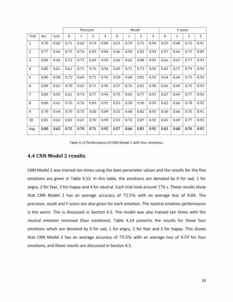
29


Trial Acc Loss 0 1 2 3 0 1 2 3 0 1 2 3

1 0.78 0.65 0.71 0.63 0.74 0.89 0.51 0.74 0.71 0.94 0.59 0.68 0.72 0.91

2 0.77 0.66 0.75 0.76 0.69 0.84 0.46 0.58 0.82 0.94 0.57 0.66 0.75 0.89

3 0.80 0.64 0.72 0.73 0.69 0.95 0.60 0.62 0.88 0.91 0.66 0.67 0.77 0.93

4 0.80 0.61 0.61 0.71 0.76 0.94 0.69 0.71 0.73 0.92 0.65 0.71 0.74 0.93

5 0.80 0.58 0.72 0.69 0.71 0.93 0.58 0.68 0.81 0.92 0.64 0.69 0.75 0.93

6 0.80 0.63 0.78 0.63 0.71 0.96 0.57 0.76 0.81 0.90 0.66 0.69 0.75 0.93

7 0.80 0.59 0.61 0.74 0.77 0.94 0.75 0.65 0.77 0.91 0.67 0.69 0.77 0.92

8 0.80 0.62 0.76 0.76 0.69 0.91 0.53 0.58 0.90 0.93 0.62 0.66 0.78 0.92

9 0.78 0.64 0.70 0.73 0.68 0.89 0.52 0.60 0.82 0.93 0.60 0.66 0.75 0.91

10 0.81 0.63 0.83 0.67 0.70 0.95 0.53 0.72 0.87 0.92 0.65 0.69 0.77 0.93

Avg 0.80 0.63 0.72 0.70 0.71 0.92 0.57 0.66 0.81 0.92 0.63 0.68 0.76 0.92

Table 4.12 Performance of CNN Model 1 with four emotions.

4.4 CNN Model 2 results

CNN Model 2 was trained ten times using the best parameter values and the results for the five

emotions are given in Table 4.13. In this table, the emotions are denoted by 0 for sad, 1 for

angry, 2 for fear, 3 for happy and 4 for neutral. Each trial took around 176 s. These results show

that CNN Model 2 has an average accuracy of 72.5% with an average loss of 0.84. The

precision, recall and F-score are also given for each emotion. The neutral emotion performance

is the worst. This is discussed in Section 4.5. The model was also trained ten times with the

neutral emotion removed (four emotions). Table 4.14 presents the results for these four

emotions which are denoted by 0 for sad, 1 for angry, 2 for fear and 3 for happy. This shows

that CNN Model 2 has an average accuracy of 79.5% with an average loss of 0.59 for four

emotions, and these results are discussed in Section 4.5.

30


Trial Acc Loss 0 1 2 3 4 0 1 2 3 4 0 1 2 3 4

1 0.72 0.85 0.68 0.77 0.65 0.85 0.57 0.57 0.78 0.55 0.92 0.64 0.62 0.77 0.60 0.88 0.60

2 0.72 0.83 0.75 0.77 0.65 0.84 0.57 0.52 0.76 0.54 0.92 0.69 0.61 0.76 0.59 0.88 0.62

3 0.73 0.83 0.74 0.71 0.67 0.88 0.57 0.51 0.74 0.55 0.93 0.71 0.60 0.73 0.60 0.90 0.63

4 0.72 0.85 0.64 0.71 0.62 0.88 0.59 0.54 0.78 0.56 0.90 0.64 0.59 0.74 0.59 0.89 0.61

5 0.72 0.85 0.67 0.76 0.64 0.89 0.54 0.57 0.75 0.60 0.85 0.68 0.61 0.75 0.62 0.87 0.60

6 0.72 0.84 0.72 0.76 0.64 0.87 0.56 0.57 0.78 0.55 0.88 0.70 0.64 0.77 0.59 0.88 0.62

7 0.72 0.86 0.63 0.77 0.65 0.88 0.55 0.54 0.75 0.52 0.90 0.71 0.58 0.76 0.58 0.89 0.62

8 0.73 0.85 0.73 0.76 0.68 0.84 0.57 0.58 0.75 0.54 0.91 0.69 0.64 0.76 0.60 0.87 0.62

9 0.71 0.83 0.73 0.78 0.62 0.87 0.53 0.53 0.74 0.52 0.89 0.71 0.62 0.76 0.57 0.88 0.61

10 0.72 0.82 0.78 0.77 0.58 0.87 0.56 0.48 0.76 0.65 0.88 0.64 0.60 0.77 0.61 0.88 0.60

Avg 0.72 0.84 0.70 0.75 0.64 0.87 0.56 0.54 0.76 0.56 0.90 0.68 0.61 0.76 0.60 0.88 0.61

Table 4.13 Performance of CNN Model 2 with five emotions


Trial Acc Loss 0 1 2 3 0 1 2 3 0 1 2 3

1 0.80 0.60 0.71 0.75 0.76 0.87 0.60 0.65 0.76 0.96 0.65 0.70 0.76 0.91

2 0.80 0.58 0.73 0.68 0.73 0.90 0.53 0.68 0.79 0.94 0.62 0.68 0.76 0.92

3 0.79 0.58 0.68 0.70 0.71 0.92 0.51 0.65 0.81 0.95 0.58 0.68 0.75 0.94

4 0.79 0.59 0.70 0.69 0.70 0.93 0.54 0.61 0.87 0.92 0.61 0.65 0.77 0.92

5 0.79 0.63 0.80 0.66 0.71 0.91 0.45 0.66 0.86 0.94 0.57 0.66 0.78 0.92

6 0.79 0.60 0.69 0.68 0.70 0.92 0.55 0.71 0.77 0.92 0.61 0.69 0.74 0.92

7 0.80 0.58 0.68 0.71 0.77 0.88 0.54 0.63 0.79 0.96 0.60 0.67 0.78 0.92

8 0.78 0.60 0.69 0.69 0.75 0.86 0.59 0.63 0.74 0.94 0.64 0.66 0.75 0.90

9 0.79 0.62 0.70 0.67 0.71 0.95 0.66 0.69 0.76 0.91 0.68 0.68 0.73 0.93

10 0.79 0.59 0.68 0.72 0.74 0.87 0.55 0.63 0.78 0.94 0.61 0.67 0.76 0.91

Avg 0.79 0.59 0.70 0.69 0.73 0.90 0.55 0.65 0.79 0.93 0.61 0.67 0.76 0.92

Table 4.14 Performance of CNN Model 2 with four emotions.

31

4.5 Comparison and evaluation of results

This section compares the performance of CNN models 1 and 2. On average, CNN Model 1

required approximately 228 s and CNN Model 2 required approximately 176 s for a trial. Table

3.2 shows that there are fewer trainable parameters in Model 2 hence it takes less time to train

than Model 1. Training with early stopping required between 80 and 100 epochs for Model 1

and between 130 and 150 epochs for Model 2. The LR for Model 2 was 0.001 and hence more

epochs were required for training than Model 1 with an LR of 0.01. With five emotions, the

average accuracy is 72.2% for Model 1 and 72.5% for Model 2. The average loss is 0.85 for

Model 1 and 0.84 for Model 2, so the results are similar. With four emotions, the average

accuracy is 80.0% for Model 1 and 79.5% for Model 2, and the corresponding average loss is

0.63 for Model 1 and 0.59 for Model 2. The accuracy is better because the models are

classifying fewer emotions. The loss is lower with Model 2 because of the slower learning rate.

Considering emotions, happy had the best performance for both models. When trained with

five emotions, happy had precision = 0.88, recall = 0.88 and F-score = 0.88 for Model 1 and

precision = 0.87, recall = 0.90 and F-score = 0.88 for Model 2. This implies that it is easier to

learn features of a happy face. This was also observed in [9], where happy had the best

accuracy for five algorithms. The neutral emotion had the worst performance for both models

with precision = 0.57, recall = 0.65 and F-score = 0.60 for Model 1 and precision = 0.56, recall =

0.68 and F-score = 0.61 for Model 2. This emotion is hard to detect since there are fewer facial

features on a neutral face. For sad, angry or fear, some facial features are consistent (lips or

forehead), and hence they are easier to learn and detect. Table 4.15 presents the performance

for five emotions and Table 4.16 gives the performance for four emotions. These results show

that performance for fear improved by approximately 7% when the model was trained with

four emotions. Fear had precision = 0.70, recall = 0.68 and F-score = 0.68 for Model 1 and

precision = 0.69, recall = 0.65 and F-score = 0.67 for Model 2 as compared to precision = 0.60,

recall = 0.63 and F-score = 0.62 for Model 1 and precision = 0.64, recall = 0.56 and F-score =

0.60 for Model 2 with five emotions. The results for sad, happy and angry are similar with four

and five emotions. However, the overall accuracy was improved and the loss reduced when

32

neutral was not considered. This shows that neutral affects the accuracy and loss of both

models.

Sad Happy Fear Angry

CNN1 CNN2 CNN1 CNN2 CNN1 CNN2 CNN1 CNN2

Precision 0.73 0.70 0.88 0.87 0.60 0.64 0.76 0.75

Recall 0.51 0.54 0.88 0.90 0.63 0.56 0.74 0.76

F-score 0.60 0.61 0.88 0.88 0.62 0.60 0.74 0.76

Table 4.15 Performance of CNN models 1 and 2 with five emotions.

Sad Happy Fear Angry

CNN1 CNN2 CNN1 CNN2 CNN1 CNN2 CNN1 CNN2

Precision 0.72 0.70 0.92 0.90 0.70 0.69 0.71 0.73

Recall 0.57 0.55 0.92 0.93 0.68 0.65 0.81 0.79

F-score 0.63 0.61 0.92 0.92 0.68 0.67 0.76 0.76

Table 4.16 Performance of CNN models 1 and 2 with four emotions.

33

4.6 Comparison of results with other emotion recognition models

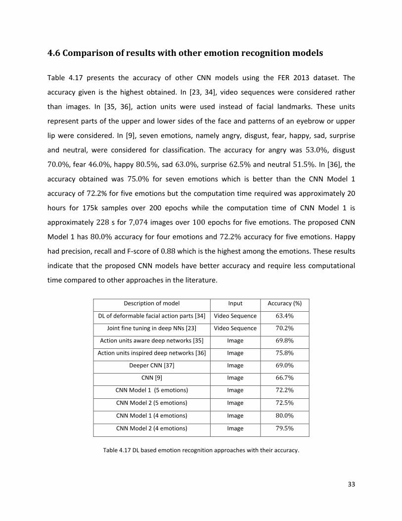
Table 4.17 presents the accuracy of other CNN models using the FER 2013 dataset. The

accuracy given is the highest obtained. In [23, 34], video sequences were considered rather

than images. In [35, 36], action units were used instead of facial landmarks. These units

represent parts of the upper and lower sides of the face and patterns of an eyebrow or upper

lip were considered. In [9], seven emotions, namely angry, disgust, fear, happy, sad, surprise

and neutral, were considered for classification. The accuracy for angry was 53.0%, disgust

70.0%, fear 46.0%, happy 80.5%, sad 63.0%, surprise 62.5% and neutral 51.5%. In [36], the

accuracy obtained was 75.0% for seven emotions which is better than the CNN Model 1

accuracy of 72.2% for five emotions but the computation time required was approximately 20

hours for 175k samples over 200 epochs while the computation time of CNN Model 1 is

approximately 228 s for 7,074 images over 100 epochs for five emotions. The proposed CNN

Model 1 has 80.0% accuracy for four emotions and 72.2% accuracy for five emotions. Happy

had precision, recall and F-score of 0.88 which is the highest among the emotions. These results

indicate that the proposed CNN models have better accuracy and require less computational

time compared to other approaches in the literature.

Description of model Input Accuracy (%)

DL of deformable facial action parts [34] Video Sequence 63.4%

Joint fine tuning in deep NNs [23] Video Sequence 70.2%

Action units aware deep networks [35] Image 69.8%

Action units inspired deep networks [36] Image 75.8%

Deeper CNN [37] Image 69.0%

CNN [9] Image 66.7%

CNN Model 1 (5 emotions) Image 72.2%




Table 4.17 DL based emotion recognition approaches with their accuracy.

34

CHAPTER 5: CONCLUSION

In this report, two CNN models were developed to extract facial features and recognize

emotions. The FER 2013 dataset was used and 7,074 images for five emotions were selected.

The emotions considered were happy, sad, angry, fear and neutral. These images were

converted into NumPy arrays and landmark features were identified and extracted. A CNN

model was developed with four phases where the first three phases had convolution, pooling,

batch normalization and dropout layers. The final phase consists of flatten, dense and output

layers. Another CNN model was developed with fewer layers. CNN Model 1 has 3,510,469

parameters of which 3,507,781 are trainable, while Model 2 has 2,734,085 parameters of

which 2,732,293 are trainable. The best parameter values were determined for these models

using the accuracy and loss metrics. Five emotions were evaluated using precision, recall and F-

score. The models were evaluated for four and five emotions. CNN Model 1 had an average

accuracy of 80.0% and average loss of 0.63 with four emotions and an average accuracy of

72.2% and average loss of 0.85 with five emotions. CNN Model 2 had an average accuracy of

79.5% and average loss of 0.59 with four emotions and an average accuracy of 72.5% and

average loss of 0.84 with five emotions. The happy emotion had the best precision, recall and F-

score of 0.88 for CNN Model 1 and precision 0.87, recall 0.90 and F-score of 0.88 for CNN

Model 2. The neutral emotion had the worst performance with precision 0.56, recall 0.64 and

F-score 0.60 for CNN Model 1 and precision 0.56, recall 0.68 and F-score 0.61 for Model 2. A

comparison with other approaches in the literature showed that the proposed models provide

better performance.

35

5.1 Future work

Facial emotion recognition is an emerging field so considering other NNs such as Recurrent

Neural Networks (RNNs) may improve the accuracy. The feature extraction is similar to pattern

recognition which is used in intelligence, military and forensics for identification purposes.

Thus, techniques such as the Capsnet algorithm for pattern recognition can be considered. DL

based approaches require a large labeled dataset, significant memory and long training and

testing times which makes them difficult to implement on mobile and other platforms with

limited resources. Thus, simple solutions should be developed with lower data and memory

requirements.

36

BIBLIOGRAPHY

[1] K. Kaulard, D.W. Cunningham, H.H. Bulthoff, C. Wallraven, The MPI facial expression database: A validated database of emotional and conversational facial expressions, PLoS One, vol. 7, no. 3, art. e32321, (2012).

[2] G.E. Hinton et al., Deep neural networks for acoustic modeling in speech recognition: The shared views of four research groups, IEEE Signal Processing Magazine, vol. 29, no. 6, pp. 82-97, (2012).

[3] A. Pentland, Social signal processing, IEEE Signal Processing Magazine, vol. 24, no. 4, pp. 108-111, (2007).

[4] M. Xie, Development of artificial intelligence and effects on financial system, Journal of Physics: Conference Series 1187, art. 032084, (2019).

[5] A. Nandi, F. Xhafa, L. Subirats, S. Fort, Real time emotion classification using electroencephalog- ram data stream in e-learning contexts, Sensors, vol. 21, no. 5, art. 1589, (2021).

[6] A. Raheel, M. Majid, S.M. Anwar, M. Alnowami, Physiological sensors based emotion recognition while experiencing tactile enhanced multimedia, Sensors, vol. 20, no. 14, art. 04037, (2020).

[7] D. Keltiner, P. Ekrman M. Lewis, J.H. Jones, Handbook of Emotions (2nd ed.), Guilford Publications (New York), pp. 236-249, (2000).

[8] O. Celiktutan, S. Ulukaya, B. Sankur, A comparative study of face landmarking techniques, EURASIP Journal on Image and Video Processing, vol. 2013, art. 13, (2013).

[9] B.C. Ko, A Brief review of facial emotion recognition based on visual information, Sensors, vol. 18, no. 2, art. 401, (2018).

[10] R. Walecki, O. Rudovic, V. Pavlovic, B. Schuller, M. Pantic, Deep structured learning for facial action unit intensity estimation, IEEE Conference on Computer Vision and Pattern Recognition, pp. 5709-5718, (2017).

[11] M.Sambhare, FER-2013 database, version 1, available online: https://www.kaggle.com/msambare/fer2013/metadata (2013).

[12] B. Zafar, R. Ashraf, N. Ali, M. Iqbal, M. Sajid, S. Dar, N. Ratyal, A novel discriminating and relative global spatial image representation with applications in CBIR, Applied Sciences, vol. 8, no. 11, art. 2242, (2018).

[13] N. Ali, B. Zafar, F. Riaz, S.H. Dar, N. Ratyal, K.B. Bajwa, M.K. Iqbal, M. Sajid, A hybrid geometric spatial image representation for scene classification, PLoS One, vol. 13, no. 9, art. e0203339, (2018).

37

[14] N. Ali, B. Zafar, M.K. Iqbal, M. Sajid, M.Y. Younis, S.H. Dar, M.T. Mahmood, I.H. Lee, Modeling global geometric spatial information for rotation invariant classification of satellite images, PLoS One, vol. 14, no. 7, art. e0219833, (2019).

[15] N. Ratyal, I. Taj, U. Bajwa, M. Sajid, Pose and expression invariant alignment based multi view 3D face recognition, KSII Transactions on Internet and Information Systems, vol. 12, no. 10, pp. 4903-4929, (2018).

[16] T. Danisman, M. Bilasco, N. Ihaddadene, C. Djeraba, Automatic facial feature detection for facial expression recognition, International Conference on Computer Vision Theory and Applications, pp. 407-412, (2010).

[17] L.A. Parr, B.M. Waller, Understanding chimpanzee facial expression: Insights into the evolution of communication, Social Cognitive and Affective Neuroscience, vol. 1, no. 3, pp. 221-228, (2006).

[18] J.M.F. Dols, J.A. Russell, The science of facial expression, Oxford University Press, vol. 13, no. 2, pp. 103-104, (2017).

[19] S.G. Kong, J. Heo, B.R. Abidi, J. Paik, M.A. Abidi, Computer vision and image understanding, Academic Press Elsevier, vol. 97, no. 1, pp. 103-135, (2005).

[20] Y.I. Xue, X. Mao, F. Zhang, Beihang University facial expression database and multiple facial expression recognition, IEEE International Conference on Machine Learning and Cybernetics, pp. 3282-3287, (2006).

[21] S.E. Kahou, V. Michalsk, K. Konda, Recurrent neural networks for emotion recognition in video, International Conference on Multimodal Interaction, pp. 467-474, (2015).

[22] D.H. Kim, W. Baddar, J. Jang, Y.M. Ro, Multi objective based spatio temporal feature representation learning robust to expression intensity variations for facial expression recognition, IEEE Transactions on Affective Computing, vol. 10, no. 2, pp. 223-236, (2019).

[23] H. Jung, S. Lee, J. Yim, S. Park, J. Kim, Joint fine tuning in deep neural networks for facial expression recognition, IEEE International Conference on Computer Vision, pp. 2983-2991, (2015).

[24] A. Mostafa, M.I. Khalil, H. Abbas, Emotion recognition by facial features using recurrent neural networks, IEEE International Conference on Computer Engineering and Systems, pp. 417-422, (2008).

[25] D.K. Jain, Z. Zhang, K. Huang, Multi angle optimal pattern based deep learning for automatic facial expression recognition, Pattern Recognition Letters, vol. 139, pp. 157-165, (2020).

[26] H.W. Ng, V.D. Nguyen, V. Vonikakis, S. Winkler, Deep learning for emotion recognition on small datasets using transfer learning, International Conference on Multimodal Interaction, pp. 443-449, (2015).

38

[27] H. Chang, Z. Liang, J. Chen, MMI dataset, version 1, available online: https://mmifacedb.eu/ (2018).

[28] W.J. Yan, X. Li, S.J. Wang, G. Zhao, Y.J. Liu, Y.H. Chen, X. Fu, CASME II: An improved spontaneous micro expression database and the baseline evaluation, PloS One, vol. 9, no. 1, art. e86041, (2014).

[29] P. Lucey, J.F. Cohn, T. Kanade, J. Saragih, Z. Ambadar, I. Matthews, The extended Cohn-Kanade dataset (CK+): A complete dataset for action unit and emotion specified expression, IEEE Computer Society Conference on Computer Vision and Pattern Recognition, pp. 94-101, (2010).

[30] M.O. Parkhi, A. Vedaldi, A. Zisserman, Deep face recognition, British Machine Vision Conference, pp. 41.1-41.12, (2015).

[31] A. Amini, A. Soleimany, MIT deep learning open access course 6.S191, available online: http://introtodeeplearning.com/ (2020).

[32] D.H. Hubel, T.N. Wiesel, Receptive fields and functional architecture of monkey striate cortex, Journal of Physiology, vol. 195, no. 1, pp. 215-243, (1968).

[33] S. Shah, A comprehensive guide to convolutional neural networks, available online: https://towardsdatascience.com/a-comprehensive-guide-to-convolutional-neural-networks-the-eli5-way-3bd2b1164a53, (2018).

[34] M. Liu, S. Li, S. Shan, R. Wang, X. Chen, Deep learning deformable facial action parts model for dynamic expression analysis, Asian Conference on Computer Vision, pp. 1-14, (2014).

[35] M. Liu, S. Li, S. Shan, X. Chen, AU-inspired deep networks for facial expression feature learning, Neurocomputing, vol. 159, no. 1, pp. 126-136, (2015).

[36] A. Mollahosseini, D. Chan, M.H. Mahoor, Going deeper in facial expression recognition using deep neural networks, IEEE Winter Conference on Applications of Computer Vision, (2016).

[37] A. Sinha, R.P. Aneesh, Real time facial emotion recognition using deep learning, International Journal of Innovations & Implementations in Engineering, vol. 1, pp. 1-5, (2019).

[38] D. Clevert, T. Unterthiner, S.Hochreiter, Fast and accurate deep network learning by exponential linear units, International Conference on Learning Representations, (2016).

[39] K. He, X. Zhang, S. Ren, J. Sun, Delving deep into rectifiers: Surpassing human level performance on imagenet classification, IEEE International Conference on Computer Vision, pp. 1026-1034, 2015.

FACIAL EMOTION DETECTION USING CONVOLUTIONAL NEURAL NETWORKS

Documents

Transcript of FACIAL EMOTION DETECTION USING CONVOLUTIONAL NEURAL NETWORKS