ECE 18-551 – Digital Communication &

Signal Processing Systems Design

Spring 2003

FACE VERIFICATION FOR ATM ACCESS

Final Report May 5th, 2003

Group 2

Zack Edmondson (zke@ece.cmu.edu)

Rohit Patnaik (rpatnaik@ece.cmu.edu)

Adam Zelinski (acz@ece.cmu.edu)

2

1. INTRODUCTION

We have designed and implemented a Face Verification system that has a low

probability of error in the presence of illumination variation. The system has been

implemented on a Texas Instruments C67 Digital Signal Processing (DSP) Board, and

runs in real time. This report describes how we implemented this system, followed by an

analysis of the results.

1.1 THE PROBLEM

The problem of authenticating oneself to acquire a good or service is common –

an example of this is withdrawing money from an Automatic Teller Machine (ATM).

Using an ATM typically involves using a Personal Identification Number (PIN). This PIN

can easily be forgotten and stolen. Millions of dollars are lost per year due to the use of

stolen PINs. Our goal, therefore, was to find a way to eliminate the usage of PINs while

still keeping the process of using an ATM timely and efficient.

1.2 THE SOLUTION

A better method of identifying a user who is attempting to withdraw money from

an ATM is by having the user present their name to the machine, and then allowing the

machine to take a picture of their face. This picture is then analyzed by the machine to

see if the name and face pair of the person requesting money actually matches up with

the name and face pair stored at a location accessible by the ATM (a database, an

identification card, etc.).

Our solution involves real-time image processing and facial verification. The

primary means of identifying name and face pairs rely on training a set of filters and

performing correlation filtering via Fast Fourier Transforms. The filters are robust in the

presence of illumination variation. Being capable of dealing with illumination variation is

crucial because people will approach the ATM at different times of the day.

3

2. PREVIOUS WORK IN THE FIELD

2.1 PREVIOUS 18-551 PROJECTS

• In Spring 2002, Group 2 did a project on Face Detection.

• In Spring 2002, Group 3’s project involved Gender and Emotion Facial

Classification.

• In Spring 2002, Group 6 did a verification project involving fingerprints.

2.2 OUTSIDE OF 18-551

• Professor B.V.K Vijaya Kumar’s Multi-Biometric Authentication System (MBAS)

group does work in Face Verification and other forms of biometric verification.

• Myriad forms of face verification software & hardware systems exist in the

commercial world. Visionic Corporation’s “FaceIt” face verification system is

particularly well-known.

2.3 UNIQUENESS

Our project is clearly different from the previous 18-551 projects, as none of them

did face verification. Our project differs from the MBAS group’s face verification system,

because their system is not implemented in DSP hardware.

Correlation filters have predominantly been used only in Automatic Target

Recognition and Synthetic Aperture Radar applications, and are not routinely used for

face verification. Most commercial face verification systems available primarily utilize

Feature Extraction and Feature Classification rather than correlation filtering techniques.

For example, the well known “FaceIt” product uses Feature Extraction and Feature

Classification. Therefore, our usage of correlation filtering for face verification is unique.

4

3. DATABASE

We used a subset of the Pose, Illumination, and Expression (PIE) Database[3].

The PIE database contains about 41,368 images and is 30 Gigabytes (GB) in size. It

contains images of 68 persons. There are 13 different poses, 43 different illumination

conditions, and 4 different expressions per person.

The subset of the PIE database that we used for our project contains 67 people.

There are 21 illumination images per person. Each subject’s pose and expression are

relatively constant across the images associated with each subject. In each image, the

individual is directly facing the camera and has a neutral expression.

The images in the PIE database are stored in portable pixmap (PPM) format and

are located on a server. We first copied all the relevant images to a separate directory,

and then we used a MATLAB® script to pre-process all these images and save them in

bitmap and JPEG formats. We also saved these images as ASCII files. This is how we

created the subset database from the original database.

3.1 IMAGES FROM THE PIE DATABASE

Figure 1: Example of images in the PIE database

[3] The CMU Pose, Illumination, and Expression (PIE) Database, T. Sim and S. Baker and M. Bsat,

Proceedings of the 5th International Conference on Automatic Face and Gesture Recognition, 2002

5

The images in Figure 1 are an example of the images from the PIE database

which we selected to be our subset. The subject’s pose is facing forward, and the

subject’s expression is neutral. The images are 640x486 pixels in size, 24-bits per pixel.

3.2 CREATION OF THE SUBSET DATABASE

The images from the PIE database were first converted to grayscale, and were

cropped to 129x129 pixels and centered based on the eye and nose coordinates

provided in the original database. They were then downsampled to 64x64 images by

averaging pixels. Down sampling the images has a dual purpose. First, it is a form of

low-pass filtering and eliminates high frequency components in the image (noise).

Second, reducing the size of the images has computational benefits. Figure 2 is an

example of the images that comprise the subset database.

Figure 2: Example of images from our subset database

6

4. SYSTEM OVERVIEW

A process flow graph of our system is depicted in Figure 3.

Train the Filters(MATLAB,

Non-Real Time)

User submits(name, face) pair

to machine(EVM-Processing,

Real-Time)

Input Data(PIE

Subset Database)

A filter now existsfor each person

(Disk Drive)EnrollmentStage

Machine waits

for input(WinNT GUIprogram)

Check whetherUser is authenticor an Imposter.

Real-TimeVerificationStage

Figure 3: Process flow graph of our system

From Figure 3 above, it is apparent that the system is comprised of 2 stages, the

Enrollment Stage and the Real-Time Verification Stage.

4.1 ENROLLMENT STAGE

The Enrollment Stage is performed offline and is performed primarily in

MATLAB®. The input to the Enrollment Stage is a selection of images from our subset

database. The subset database is described above in section 3.

During the Enrollment Stage, a correlation filter is created for each individual

enrolled in the database – since there are 67 people in our subset database, 67 filters

are created. The specifics behind correlation filtering and two specific filter algorithms,

MINACE and EMACH, are described in section 5. The training method for creating the

filters is described in section 6 – this section includes information on the system testing

set, the training set, and explores the two filter algorithms in detail. In section 7, the

optimal filter algorithm is chosen for the system.

7

4.2 REAL-TIME VERIFICATION STAGE

The Real-Time Verification Stage is distinct from the Enrollment Stage. This

stage makes use of the filters created during the Enrollment Stage. Given an input

image and a user name (e.g., the {name, face} pair as written in Figure 3), the system

performs a correlation using the stored filter corresponding to the particular input name.

The system uses the correlation result to determine whether the input image

corresponds to that name. The system then returns a message indicating whether the

user was authenticated or was recognized as an imposter. Section 8 describes the

hardware implementation of our system on the Texas Instruments C67 device – this

includes relevant information on memory allocation, code optimization, and profiling of

the system’s code.

4.3 PERFORMANCE & DEMONSTRATION OF THE SYSTEM

Section 9 of this report describes the performance (e.g., the number of errors) of

our system – it illustrates this via a confusion matrix. Section 10 describes our

demonstration system, describing the system’s Graphical User Interface (GUI) in detail.

5. ALGORITHMS

Our system is based on using correlation filtering to determine whether a subject

is an authentic user or an imposter. We choose to evaluate two types of distortion

invariant filters for our project. These are the MINACE (minimum noise and average

correlation plane energy) filter, and the EMACH (Extended Maximum Average

Correlation Height) filter.

Noise plays an important part in face verification and in sub-section 5.1, we

describe the noise model we chose and the reason for choosing it. In sub-sections 5.2

and 5.3, we describe the theory behind these filters and their implementation. In sub-

8

section 5.4, we describe the process of choosing the peak and (peak-to-sidelobe ratio

(PSR) thresholds, which help in determining whether the user is authentic or an

imposter. PSR is described in that sub-section. The method for determining whether a

given image is that of an authentic person or an imposter is described in sub-section 5.5.

5.1 NOISE CONSIDERATIONS

Noise alters a filter’s recognition and discrimination capabilities. We assumed an

Additive White Gaussian Noise (AWGN) model. This is a good model of in-plane

distortion. We assumed that the white noise two-sided power spectral density variance is

one (1) without any loss of generality as is mentioned in[2]. This means that the noise has

equal energy at all frequencies.

5.2 MINACE

MINACE (minimum noise and average correlation plane energy) distortion-

invariant filters have proven very attractive for detection and recognition of objects in

infrared and SAR imagery[1]. We have attempted to use this filter for our application,

which deals with verification in the presence of illumination variation. The MINACE filter

minimizes a combination of Correlation Plane Signal Energy (ES) and Correlation Plane

Noise Energy (EN). The filter is required to give correlation plane values of 1 at the origin

for each training set image; this is known as the peak constraint.

Reducing only ES subject to the peak constraint produces delta-function-like

correlation peaks. This reduces correlation plane sidelobes and hence localizes the

object well in the correlation plane. To achieve this, the filter emphasizes high spatial

[2] Improving the false alarm capabilities of the maximum average correlation height

correlation filter. Alkanhal, Vijaya Kumar, Mahalanobis, Proc. Opt. Eng. 39(5), 1133-1141 (2000) [1] Distortion-Invariant FOPEN Detection Filter Improvements, Casasent, Ippolito and Verly, Proc.

SPIE, vol. 3721, April 1999 conference

9

frequencies in the object data. Hence, minimizing ES tends to reject imagery not present

in the training set; i.e. it minimizes false alarms, but can make detection of test set

images not present in the training set difficult.

Minimizing EN emphasizes lower spatial frequencies and thus improves the

probability of detection (PD) while making the probability of false acceptance (PFA)

worse. Minimizing the combination E = ES + cEN for a suitable value of c is thus

preferable. The method for choosing c is described in the following paragraphs. Some of

the information in the following paragraphs has been taken from [1].

We denote vectors (matrices) as lower (upper) case bold letters. All data are

Fourier Transform (FT) data, as synthesis is easier. The FT of the filter is h (all vectors

are one-dimensional lexicographically ordered two-dimensional data). The columns of

the data matrix X are the FTs of the training set images (different illumination images of

a subject). We require the filter to give correlation plane values of 1 for each training set

image; this peak constraint is described by

XHh = u = [1,…,1]T – (i)

where ()H denotes conjugate transpose and the elements of the vector u are specified

correlation peak values for the different illumination images. As stated previously, we

wish to minimize the combination

E = ES + cEN

The above represents the objective function which the filter h is required to minimize.

The control parameter is chosen to emphasize minimization of ES or EN. The correlation

plane energy due to all training set images is

ES = hHSh

[1] Distortion-Invariant FOPEN Detection Filter Improvements, Casasent, Ippolito and Verly, Proc.

SPIE, vol. 3721, April 1999 conference

10

This is the energy leaving the matched spatial filter in an FT correlator, where S is a

diagonal matrix whose entries are the average spectrum of the full set of training set

images. The correlation plane energy due to noise is similarly

EN = hHNh

where the elements of the diagonal matrix N are the variance s2N of the noise model.

Since we chose an AWGN model with unit variance the diagonal elements of the N are

all 1. Thus,

E = hHSh + c(hHDh) – (ii)

The Lagrange multiplier solution that satisfies (i) and minimizes (ii) is

h = T–1X(XHTX)u, where

T = max[S1(u, v), S2(u, v),…,cN] = envelope at each frequency (u, v), and

c = (dc of N) / (dc of S) = s 2N / S(0, 0)

This is how the MINACE filter is created.

5.3 EMACH

The maximum average correlation height (MACH) correlation filter

overemphasizes the importance of the average training image leading to poor

discrimination of the desired class images from the clutter images. To overcome this,

two metrics termed All Image Correlation Height (AICH) and the Modified Average

Similarity Measure (MASM) are optimized in the EMACH (extended maximum average

correlation height) filter. Most of the information in the following paragraphs has been

taken from [2].

AICH = ∑=

N

iN 1

1 (h+xi)2 – a(h+xi)2, – (i)

[2] Improving the false alarm capabilities of the maximum average correlation height

correlation filter. Alkanhal, Vijaya Kumar, Mahalanobis, Proc. Opt. Eng. 39(5), 1133-1141 (2000)

11

where a is a parameter that takes on a value between 0 and 1 and governs the relative

significance of the average training image in the filter design. The superscript +

represents the complex conjugate transpose. It is easy to show that AICH in Eq. (i) can

also be written as

AICH = ∑=

N

iN 1

1 [h+(xi – ßm)] 2

= ∑=

N

iN 1

1 (h+xi – ßh+m) 2

= ∑=

N

iN 1

1 (h+xi)2 – (2ß – ß2)(h+m) 2, – (ii)

provided a = 2ß – ß2. Equivalently, a and ß are related by αβ −±= 11 . Thus as a

varies between 0 and 1, ß varies between 0 and 2. From here on, we refer only to ß and

ignore a. By controlling ß, the designed filter is prevented from being overwhelmed by

the biased treatment of the low-frequency components represented by the average

image. Here, AICH must be optimized. To be able to do that, we write Eq. (ii) as

AICH = ∑=

N

iN 1

1 (h+xi – ßh+m) 2

= ∑=

N

iN 1

1 (h+xi – ßh+m) (h+xi – ßh+m)+

= h+[ ∑=

N

iN 1

1 (xi – ßm) (xi – ßm) ] h

= h+Cxßh, – (iii)

where

Cxß = ∑

=

N

iN 1

1 (xi – ßm) (xi – ßm)+, – (iv)

12

Thus, as shown in Eq. (iv), AICH can be described as the average of the correlation

peak intensities of N exemplars where the ith exemplar (xi – ßm) is the ith training

images with part of the mean subtracted. Hence, it is desirable for all the images in the

training set to follow the behavior of these exemplars. This can be done by forcing every

image in the training set xi to have a similar correlation output plane to an ideal

correlation output shape f. To find the f that best matches all these exemplar’s

correlation output planes, we minimize its deviation from their correlation planes. This

deviation can be qualified by the average squared error (ASE):

ASE = ∑=

N

iN 1

1 (gi – f)+(gi – f) , – (v)

where

g = (Xi – ßm)h*, – (vi)

where the superscript * represents the complex conjugate.

To find the optimum shape vector fopt, we set the gradient of ASE with respect to

f to zero. Then, we obtain

fopt = ∑=

N

iN 1

1 gi

= ∑=

N

iN 1

1 (Xi – ßM)h*

= (1 – ß)Mh*, – (vii)

Now, we modify the Average Similarity Measure (ASM) such that it measures the

dissimilarity of the training images to (1 – ß)Mh*. We call the new measure the modified

ASM (MASM).

MASM = ∑=

N

iN 1

1 [(Xih*– (1 – ß)Mh*]+ [(Xih*– (1 – ß)Mh*]

13

= hT ∑=

N

iN 1

1 [(Xi – (1 – ß)M]*[(Xi – (1 – ß)M] h*

= hTSxßh

= h+Sxßh, – (viii)

where the superscript T represents the transpose and where we used the fact that

MASM is real in deriving the last equality in Eq. (viii). The diagonal matrix Sxß is given by

Sxß = ∑

=

N

iN 1

1 [(Xi– (1 – ß)M]*[(Xi– (1 – ß)M], – (ix)

As we know, the ASM is a good measure for distortion tolerance; however, it lacks some

discrimination capability that explains part of the EMACH filter’s inability to reject some

clutter images. On the other hand, the MASM measure captures finer details of the

training set that makes the new designed filter more sensitive against clutter. This can

be more easily see when Eq. (viii) is rewritten as

MASM = hT( ∑=

N

iN 1

1 Xi*Xi )h – (1 – ß2)h+M*Mh

= h+Dxh – (1 – ß2)h+M*Mh. – (x)

As we increase ß, the MASM measure emphasizes the Average Correlation

Energy (ACE) term h+Dxh, and thus the influence of high-frequency components is

maximized compared to the ASM measure.

By maximizing the AICH (i.e., balancing the significance of the training frequency

components) and minimizing the MASM while controlling the parameter ß, we hope to

explicitly keep a balance between the distortion tolerance and clutter rejection

performance. Therefore, we optimize the following criterion:

Jß(h) = AICH / (h+h + h+Sxßh)

= h+Cxßh / (h+(I + Sx

ß)h) – (xi)

14

where h+h is the ONV (output noise variance) term assuming an AWGN with unit

variance. ONV helps maintain noise tolerance when ß increases especially at those low

energy components.

By maximizing the preceding criterion, we get the following condition for the

EMACH filter

(I + Sxß)–1Cx

ßh = λh, – (xii)

where λ is a scalar identical to Jß(h).

Thus, h must be an eigenvector of (I + Sxß)–1Cx

ßh with the corresponding

eigenvalue λ. Since λ is identical to Jß(h), h should be the eigenvector that corresponds

to the maximum eigenvalue. The other eigenvectors corresponding to the other nonzero

eigenvalues provide smaller Jß(h) values. However, they may provide better

discriminatory performance, as ß is not beforehand. A computational method for

determining these eigenvectors and their corresponding eigenvalues of Eq. (xii) can be

found in[4]. The following is our MATLAB® code which uses this method to create an

EMACH filter. It contains a good description of this computationally efficient method.

function H = emach(tr_imgs, beta) if (beta < 0) | (beta > 2) disp('beta must be between 0 and 2'); disp('Exiting function...'); return; end num_imgs = size(tr_imgs, 2); [m, n] = size(tr_imgs{1}); d = m*n; % X is the data matrix. The columns of X contains the FT of the training images X = zeros(d, num_imgs); for i = 1:num_imgs img_i = tr_imgs{i}; %img_i = img_i/norm(img_i, 'fro'); fft_img_i = fft2(double(img_i)); X(:,i) = fft_img_i(:); end

[4] Distance-classifier correlation filters for multiclass target recognition, A. Mahalanobis, B.V.K.

Vijaya Kumar, and S.R.F. Sims, Appl. Opt. 35(17), 3127-3133 (1996)

15

% Obtain the average FT of all training images M = mean(X, 2); X_diff = X - (1-beta)*repmat(M, 1, num_imgs); % S_B S_B = mean(X_diff.*conj(X_diff), 2); % % Compute the eigenvector corresponding to the largest eigenvalue % % (1 + S_B)^(-1)C_B*H_tmp = lambda*H_tmp % The following is an efficient method to compute the dominant eigenvector % C_B = (1/num_images)*YY' Y = X - beta*repmat(M, 1, num_imgs); % Since the inner-product matrix Z = Y'*Y is symmetric and positive definite % Z = Y'*Y = V*D*V' [V, D] = eig(Y'*Y); % It can be shown that C_B has the same num_images non-zero eigen values % and (d - num_images) zero eigenvalues % The eigenvectors of C_B corresponding to the non_zero eigenvalues can be % shown to be the columns of the dxnum_images matrix phi, where phi = Y*V*D^(-1/2); Noise = ones(d, 1); % S_inv_phi = diag(S_B.^(-1))*phi; S_inv_phi = phi./repmat(Noise + S_B, 1, num_imgs); % delta*phi'S^(-1)*phi tmp = D*phi'*S_inv_phi; [e, lambda] = eig(tmp); [max_lambda, max_index] = max(abs(diag(lambda))); % Compute H_tmp H_tmp = (phi./repmat(Noise + S_B, 1, num_imgs)) * e(:, max_index); % Obtain H H = d*d*reshape(H_tmp, m, n);

This concludes our description of the EMACH filter algorithm.

5.4 DETERMINING THE PEAK AND PSR THRESHOLDS

5.4.1 PEAK-TO-SIDELOBE RATIO (PSR)

One of the primary concerns in face verification is the detectability of the

correlation peak. It is important for the correlation peaks to be sharp enough. A good

measure for the peak sharpness is the peak-to-sidelobe-ratio (PSR):

PSR = (peak – mean) / standard deviation

= (p – µ) / s,

16

where p is the peak of the correlation output, and µ and s are the mean and standard

deviation, respectively, of the sidelobe region. We chose the sidelobe of the correlation

plane to be the region outside a 5x5 block and within a 20x20 block centered at the

peak.

5.4.2 COMPUTING THE PSR

The following describes our algorithm for computing the PSR for a correlation plane.

1. Find the peak of the correlation plane.

2. If the peak lies within 10 pixels of any boundary, then the

peak is too shifted, and a PSR of 0 is returned.

3. We compute the mean, and the standard deviation (std) of

the sidelobe region.

4. The PSR is returned as (peak – mean) / std.

5.4.3 FINDING THE THRESHOLDS

5.4.3.1 MINACE

The following algorithm describes how we chose the peak and PSR thresholds for

the MINACE filter:

1. Correlate the MINACE filter for a particular subject

against all images of the same subject and find the minimum

peak (minPEAK) and minimum PSR (minPSR) values of the

correlation planes.

2. The peak threshold (peakTH) is set as 0.9*minPEAK.

3. Correlate the same filter against all the images in the

subset database that are not the subject’s images, and find

the peak and PSR values for the correlation planes.

17

4. For all correlation planes in step 2 for which the peak

exceeds peakTH, find the maximum PSR (maxPSR) for those

correlation planes .

5. If maxPSR exceeds minPSR, then the PSR threshold (psrTH) is

returned as minPSR.

5. Otherwise, psrTH is returned as (minPSR + maxPSR)/2.

We chose this method to set the peak and PSR threshold because by iteratively setting

the thresholds and evaluating the performance of the system, we would have arrived at

thresholds which would be similar to those obtained using this method.

5.4.3.2 EMACH

The following algorithm describes how we chose the peak and PSR thresholds for

the EMACH filter:

1. Correlate the EMACH filter for a particular subject against

all images of the same subject and find the minimum peak

(minPEAK) and minimum PSR (minPSR) values of the

correlation planes.

2. The peak threshold (peakTH) is set as 0.9*minPEAK.

3. The PSR threshold (psrTH) is set as 0.95*minPSR.

We chose this method to set the peak and PSR threshold because by iteratively setting

the thresholds and evaluating the performance of the system, we would have arrived at

thresholds which would be similar to those obtained using this method.

5.5 DETERMINING AUTHENTICITY OF A {NAME, FACE) PAIR

The following describes our algorithm for determining the authenticity of an input image

using either the MINACE or the EMACH filer:

18

1. Given an input and a {name, face} pair, correlate the

filter corresponding to the name part of the {name, face}

pair with the image, and find the correlation output.

2. If the peak and PSR of the correlation output are both not

less than the respective thresholds for that filter, then

the input is considered to be from an authentic subject,

else it is considered to be from an imposter.

6. TRAINING AND TESTING

Our subset database contains 21 images per person. These range from left

illumination to full illumination to right illumination. An example of the images for one

person is shown in Figure 4. As can be seen, there is a significant variation in

illumination across the 21 images. The training and test set are taken from this

database. The training and testing method for the MINACE and EMACH filters is

described below.

Figure 4: 21 Illumination images for one subject

19

6.1 TRAINING

6.1.1 MINACE

We used 3 images per person – left illumination, right illumination, and full

illumination – to create a filter for each person. Figure 5 shows the training set for

creating the MINACE filter for one subject. Since the MINACE filter is based on

minimizing the correlation plane signal and noise energy, the input images for creating

the filter are normalized such that each has unit energy.

As is intuitive, these images are most representative of the different kinds of

illumination variation in the subset database. B By using only these 3 images for every

person, we achieved very good results in the testing stage (which is described in section

6.2.1). As was described in the MINACE algorithm, the parameter c used to create the

MINACE filter is determined heuristically. The value of the parameter c for the filters for

all the subjects in shown in Figure 6.

Figure 5: Images used to create the MINACE filter for a particular subject

20

Figure 6: Values of the parameter c used for the MINACE filters

6.1.2 EMACH

The training images used to create the EMACH filter are not normalized. This is

because the EMACH filter is based on making the correlation plane of the image similar

to that of the mean image. This does not involve energy considerations. Normalizing the

image for this filter actually leads to worse performance in the testing stage.

Initially, we used the same training images that we used for creating the MINACE

filters. However, the resulting EMACH filters performed poorly both on intra-class and

inter-class data, leading to significantly high false rejection and false acceptance rates.

We wanted to keep the images with left and right illumination, since they represent

extremes in illumination. After some testing, we found that including the image with

21

complete illumination was leading to poor performance, since this image was dominating

the other two while making the filter.

We then decided to use the images depicted in Figure 7. This training set

includes the left and right illuminated images. Notice, the image with full illumination has

been replaced by two images with nearly full illumination but one is brighter on the right

side of the face while the other is brighter on the left. This training set results in filters

that exhibit much better performance than was obtained using the previous training set.

The detrimental dominating effect of the fully illuminated face image has been eliminated

by using two less-brightly illuminated images in its place.

Figure 7: Images used to create the EMACH filter for a particular subject

We used different values of the parameter ß to create the EMACH filters and

then tested their performance on the test set. As the value of ß increased, the

performance of the EMACH filters worsened.

6.2 TESTING

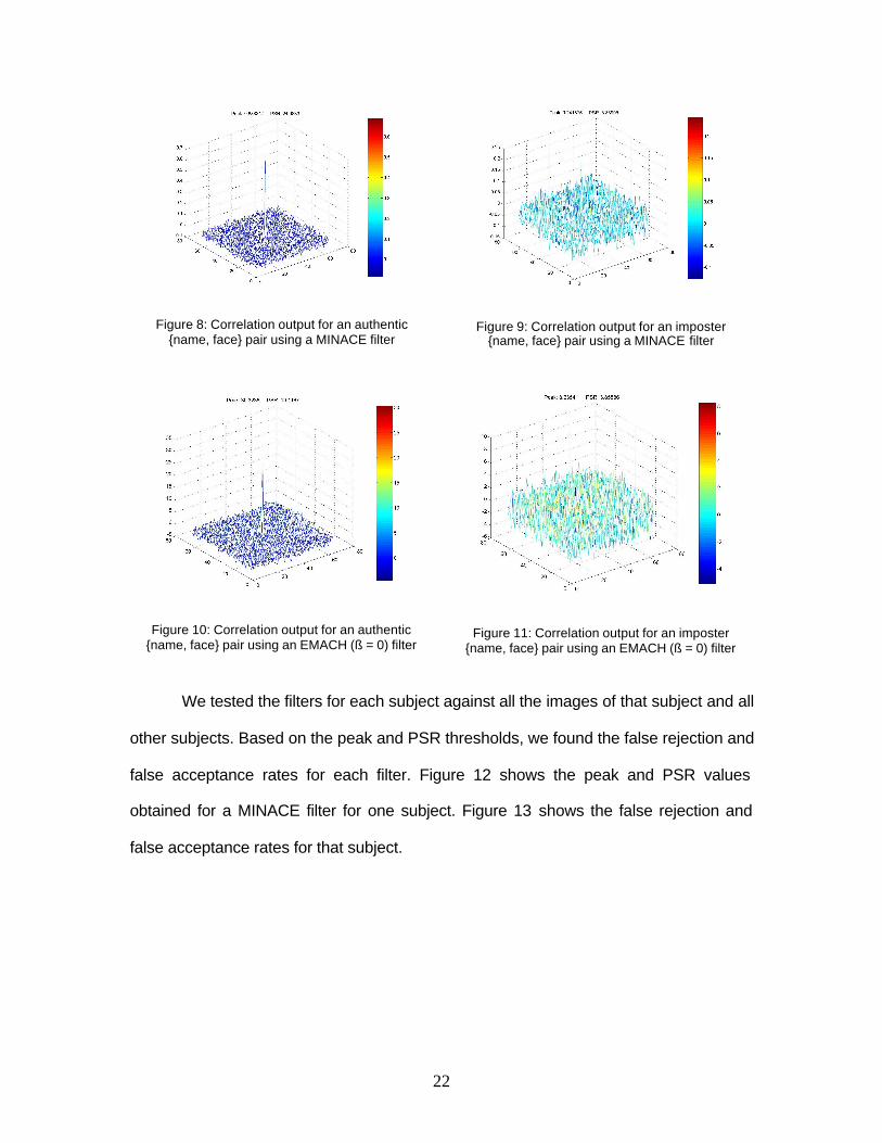
The test set consists of all the images. Figures 8-11 show examples of

correlation outputs using a MINACE filter and an EMACH filter with ß = 0.

22

Figure 8: Correlation output for an authentic {name, face} pair using a MINACE filter

Figure 9: Correlation output for an imposter {name, face} pair using a MINACE filter

Figure 10: Correlation output for an authentic {name, face} pair using an EMACH (ß = 0) filter

Figure 11: Correlation output for an imposter {name, face} pair using an EMACH (ß = 0) filter

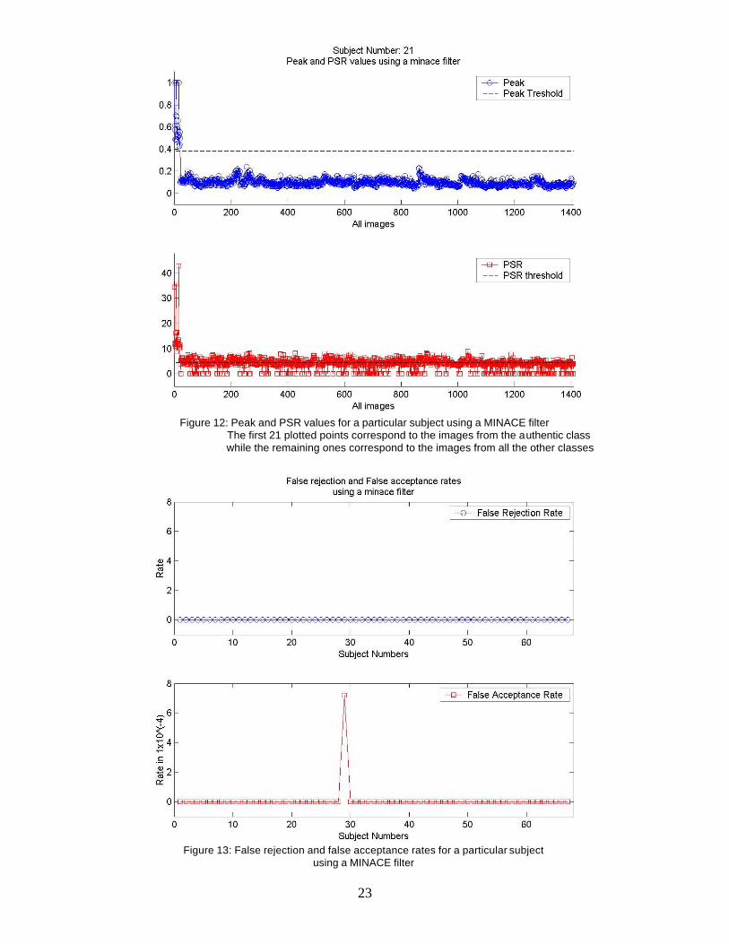
We tested the filters for each subject against all the images of that subject and all

other subjects. Based on the peak and PSR thresholds, we found the false rejection and

false acceptance rates for each filter. Figure 12 shows the peak and PSR values

obtained for a MINACE filter for one subject. Figure 13 shows the false rejection and

false acceptance rates for that subject.

23

Figure 12: Peak and PSR values for a particular subject using a MINACE filter The first 21 plotted points correspond to the images from the authentic class

while the remaining ones correspond to the images from all the other classes

Figure 13: False rejection and false acceptance rates for a particular subject

using a MINACE filter

24

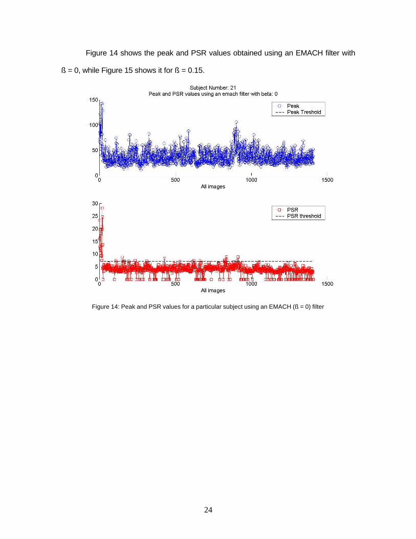
Figure 14 shows the peak and PSR values obtained using an EMACH filter with

ß = 0, while Figure 15 shows it for ß = 0.15.

Figure 14: Peak and PSR values for a particular subject using an EMACH (ß = 0) filter

25

Figure 15: Peak and PSR values for a particular subject using an EMACH (ß = 0.25) filter

Figures 16 and 17 show the false rejection and false acceptance rates for those

values of ß. As one can see from Figures 16 and 17, the performance of the EMACH

filter is worse for ß = 0.15. Larger values of ß consistently resulted in poor performance,

Based on this observation, we chose the minimum value of ß possible, which is 0.

26

Figure 17: False rejection and false acceptance rates for a particular subjectusing an EMACH (ß = 0.25) filter

Figure 16: False rejection and false acceptance rates for a particular subject using an EMACH (ß = 0) filter

27

6.3 TRAINING AND TESTING SOFTWARE

In order to perform training and testing on both types of filters, we chose to use

the celebrated MATLAB® package, which is the premier linear algebra software tool in

the twenty-first century. We also rely on MATLAB® to generate the plots presented in

this report. Due to the large number of files used (approximately 75), it is impractical to

list the description of each file. The MATLAB® code is well-commented and can be

found in the WINZIP® file, Code.zip.

The files are divided into 6 main types:

• Read_xxx – These files are used to read in different types of data stored in the

form of ASCII files.

• Write_xxx – These files are used to write different types of data to ASCII files.

• Display_xxx – These files are used to display the various plots included in this

report.

• Convert_xxx – These files are used to convert the relevant images from the PIE

database, which are stored in ppm format, to bitmap, JPEG and ASCII files as

required.

• Helper Files – These files perform tasks such as creating the filters, extracting

relevant information from correlation results, and generating data used to create

the plots in this report.

• Test – These files are used to test the performance of the filters for intra-class

and inter-class images. They played an important role in choosing the filter

parameters.

28

7. FILTER COMPARISON

Using the false rejection and false acceptance rates, examples of which were

shown in section 6, we determined that the performance of the MINACE filter was far

better than the performance of the EMACH filter. The only EMACH filter with

performance comparable to that of the MINACE was the one with ß = 0. Even for this

filter, the false rejection rates were higher than those for the MINACE filter. We made

these decisions based on testing on all the images in our subset database.

8. SOFTWARE AND HARDWARE IMPLEMENTATION OF THE SYSTEM

8.1 SIGNAL FLOW (PC & EVM)

This subsection describes the signal and processing flow of our system during

the Real-Time Verification Stage. The detailed signal flow of the system during this stage

is illustrated in Figure 18.

PC-SideProcess(GUI)

is initialized.

The PC-Side process receives the result from the EVM,

and the GUI program spawns an Authentic or Imposter

window showing the result to the user.

User submits(name, face) pair for authentication

by using GUI.

1) Filter associated with input name.

2) Correlation Peak threshold value associated with input name.

3) PSR threshold value associated with input name.

4) Input face image.

EVM Processing occurs in Real-Time

(See Figure 19);Authentic or Imposter

flag is sent back to the PC.

PC-SideProcess sends 4 pieces of data to the EVM.

The system runs in a loop.

Figure 18: Signal Flow – PC & EVM. The system runs in a loop, performing verification in real time.

29

From this point onward we will refer to the Texas Instruments C67 Hardware

board as the Evaluation Module (EVM).

Software on a Windows Personal Computer (PC) runs a GUI and a small PC-

side process. This GUI and PC-side program allow a {name, face} pair to be submitted

to the system by a user logged into the PC. Four pieces of data are sent from the PC to

the EVM based on the chosen {name, face} pair: (1) the 64x64 filter associated with the

input name, (2) the scalar correlation peak threshold value associated with the input

name (a float), (3) the PSR threshold value associated with the input name (a float), and

(4) the 64x64 chosen input face image. The data is sent from the PC to the EVM via the

PCI bus. The PCI bus is a reliable, efficient way to transfer data to the EVM.

The EVM then performs the necessary processing steps on the filter and image.

These processing steps make up the signal flow of the EVM, which is depicted in Figure

19. The first step performed by the EVM is a 2-dimensional Fast Fourier Transform

(FFT) on the input face image. The second step is to perform a point-by-point

multiplication of the FFT’d image with the input filter, which performs a correlation via

multiplication in the frequency domain. Next, a 2-dimensional Inverse FFT (IFFT) is

performed on this result, bringing the data back into the time domain. Then, the

correlation peak is determined and its height is calculated. The PSR around the

correlation peak is calculated. Then, by comparing the correlation peak value and the

PSR value with the two input threshold values (the input correlation peak threshold value

and the input PSR threshold value, respectively), the EVM is able to decide whether the

{name, face} pair it has just processed is authentic or is an imposter.

30

Figure 19: Signal Flow – Inside the EVM. Dark colored arrows represent inputs from the PC to the EVM.

The rightmost horizontal arrow represents an output from the EVM to the PC.

After the EVM has completed these steps, it sends a message to the PC-side

program using the PCI bus. This integer value tells the PC-side program whether the

{name, face} pair has been authenticated or has been recognized as an imposter.

Finally, based on this received integer value, the GUI program displays a window which

clearly indicates the system’s decision regarding the user’s chosen {name, face} pair.

8.2 WHAT PLANS CHANGED REGARDING EVM USAGE?

Initially we had planned to store all 67 filters (one for each user) on the EVM, in

its off-chip memory region. However, we decided against doing this and currently send a

single filter to the EVM whenever that filter is needed for a particular {name, face}

verification request. Why do we not store all the filters on the EVM board? To fully

simulate the ATM system, we needed to have the ATM acquire the filter from a

“database” or “identification card”, e.g., an external source provided at the time of

verification (see section 1). Therefore, storing all the filters on the EVM would go against

the nature of the project. Furthermore, by requiring the filter to be sent to the EVM

whenever a verification is requested, this forces us to pay close attention to data

processing and data transfer. It made achieving real-time processing more of a

challenge.

2D FFT X 2D IFFT

Filter - Frequency Domain (64x64)

Decision Module

Input Peak & PSR Values (two Floats)

Authentic/Imposter Message sent to PC (Integer) Image

(64x64)

31

8.3 CODE SIZE

8.3.1 PC CODE SIZE

The size of our code on the PC side of our system is approximately 35MB. We

made no effort to minimize the size of this code, because the PC has a copious amount

of memory. Furthermore, the set of test images constitutes the largest portion of this

memory, and there was nothing we could do to reduce the size of this information.

8.3.2 EVM CODE SIZE

Our program initially contained many instances of the C function printf. This

ubiquitous function pervades all aspects of interactive debugging in the modern era. By

removing all instances of this and similar functions that were put in for the sole purpose

of debugging, our program was compact enough in size to fit entirely within the EVM’s

on-chip memory. The program totaled approximately 32 KB in size.

8.4 MEMORY ALLOCATION, DATA TRANSFERS

The EVM’s executable code is stored in on-chip memory.

Each image and filter requires 32 KB of space. As the EVM receives the image

and the filter from the PC via synchronous PCI transfers, it stores them into the 256 KB

SBSRAM (the EVM’s off-chip memory). Rows and columns of the image are then paged

to the EVM’s 128 KB on-chip memory in order to maximize the speed of the FFT of the

image. This same paging method is used when performing the point by point multiply

(the correlation in the frequency domain) and also when performing the IFFT. We used

basic core memory transfers instead of DMA, which were not applicable for our

application because transferring columns of the data required accessing non-sequential

elements of memory.

To minimize the memory footprint, the FFT, point by point multiply, and IFFT are

performed in-place.

32

8.5 CODE OPTIMIZATION

8.5.1 PARALLELIZATION

The most significant computational costs in our algorithm involved data transfer

from PC to EVM and calls to the FFT function, neither of which can be sped up by

manual loop unrolling or parallelizations in the calling code. Hence, we did not attempt

to exploit the parallel architecture of the EVM board in our own code. We comment that

TI’s FFT assembly code is written to exploit this parallel architecture already.

8.5.2 OTHER OPTIMIZATIONS

The only specific code optimization method we employed was paging. Because

the image and filter data were stored in the slower off-chip SBSRAM, it was faster to

page the memory to on-chip memory before performing the FFT’s. We estimate that this

paging saved around 5 million cycles.

We had to compile with the optimization setting “-o1” because higher levels of

optimization did not compile reliably. Specifically, the compiler would crash, freeze, or

Code Composer would generate errors when we attempted to load the output file onto

the EVM.

Because our code was fast enough for its specific practical application, we did

not consider alternative means of optimization

33

8.6 PROFILING

Table 1 characterizes the breakdown of computation required for each significant

stage of the verification process:

Operation Cycles Required PCI Transfer of the Image 2 million PCI Transfer of the Filter 2 million FFT of the Image 2 million Multiplication of Image and Filter (Frequency-Domain Correlation)

1 million

IFFT 2 million FFT Shift 1.5 million Peak Detection and PSR Computation: .5 million Total 11 million

Table 1: Approximate Cycle Counts

We comment that the profiler was unreliable and often gave widely varying

results from one trial to the next. For this reason, the figures mentioned in the table

should be recognized only as rough approximations. However, the verification occurs

fast enough that the actual user experiences no delay when using the software.

8.7 CODE USAGE & REFERENCES

In this section we outline our software and provide code references. A reference

next to a code filename appears next to all code used from external sources. Code

filenames without a reference indicate we wrote the code ourselves.

8.7.1 ENROLLMENT STAGE CODE

This code was written in MATLAB® and has been described section 6.3.

8.7.2 REAL-TIME VERIFICATION STAGE CODE

8.7.2.1 PC-SIDE CODE

The PC side code, developed in Microsoft Visual C++, was based off of

Microsoft’s “Hello World” examples available within Visual Studio. We modified the

34

generated code for this small graphical user-interface to suit our needs. A number of the

files are generated and managed by Visual Studio and are not ever edited or even seen

by the user, so we list here primarily the files we had to work with.

Testgui.cpp Includes dialog box management, file I/O, and EVM transaction code.

Testgui.rc Contains layout information for all the dialog boxes as well as needed

information regarding the images to be displayed in the GUI.

In addition to the above files, a number of generated files existed in the project; however,

we did not have to edit or understand them to effectively implement the graphical user

interface for out test program. All the files can be found in the WINZIP® file Code.zip.

8.7.2.2 EVM-SIDE CODE

We used the code provided for Lab 2 as a template for our code. Significant

changes were made, of course, to accommodate the image processing aspects of our

verification algorithm. The following list of files depicts the important C files that run on

the EVM.

fft.c/h Contains int main and serves as the primary file for the EVM side. All

calls to DSP functions (FFT, PSR calculation, etc.) are made from this

file.

PSR.c/h Contains functions for detecting the peak and calculating the PSR. These

were developed separately from the rest of the code to simplify

debugging stages.

35

Cfftr4.asm TI’s own hand-coded assembly which implements a radix 4 FFT. This file

is available at the Texas Instruments website [5].

8.8 “EVM ~= MATLAB®”

All of the results produced by the EVM, such as correlation outputs, peak

determinations, and PSR calculations, approximately match those computed by

MATLAB®. The differences between EVM and MATLAB® results are on the order of

one-hundred thousandths (10-5). This minute difference in computation occurs because

the EVM performs calculations using data of type float and MATLAB® uses data of type

double. Recall that a float is 4 bytes in size, whereas a double is 8 bytes in size. It is

clear that a double has more numerical accuracy than a float. This explains the

miniscule differences in EVM and MATLAB® results, and why this difference is not an

issue of concern.

Since our system, when simulated in MATLAB®, produces the same results as

when using the EVM, we have performed all of our confusion matrix calculations via

MATLAB® scripts. This is clearly acceptable based on the above discussion of EVM vs.

MATLAB® results.

8.9 SOFTWARE & HARDWARE IMPLEMENTATION – CONCLUDING REMARKS

Clearly, from our discussion above, the EVM performs the majority of the

processing. The software process which runs on the PC-side of the Real-Time

Verification Stage is minimal and is only used to run the GUI, send data to the EVM, and

show results to the user. Therefore, we put the most amount of processing steps onto

the EVM as was possible given our system’s design.

[5] Texas Instruments website: http://www-k.ext.ti.com/sc/technical-support/tools/dsp/ftp/c67x.htm

36

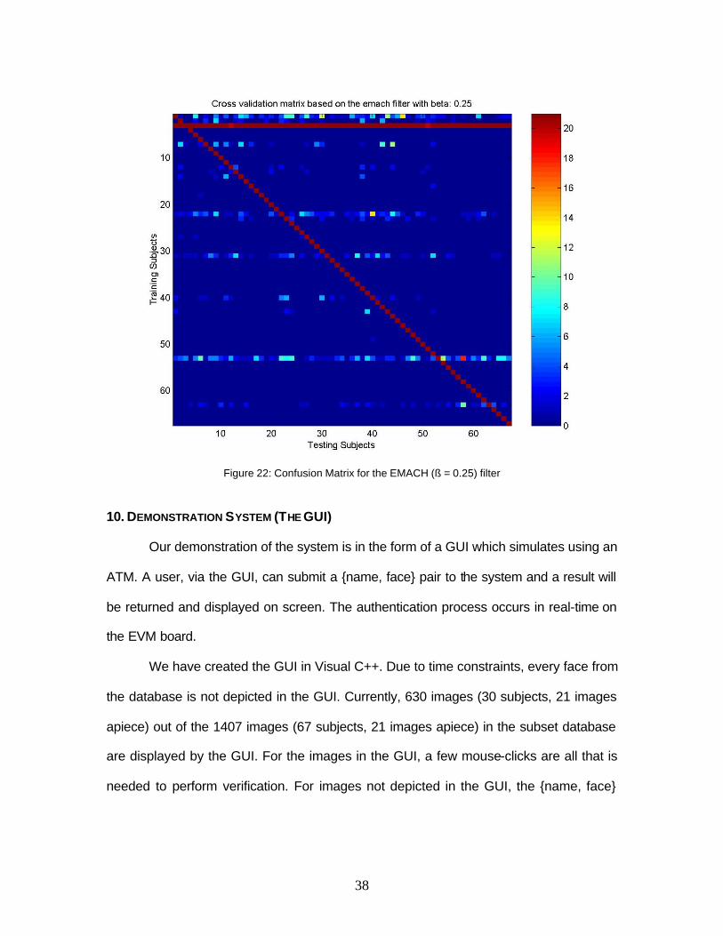
9. ERROR PERFORMANCE ANALYSIS

We computed confusion matrices for the MINACE filter and for the EMACH filter

for different values of ß. Figures 20, 21 and 22 contain the 2-D image plot of these

matrices generated with the MATLAB® command imagesc. This is how we created the

confusion matrices :

1. Correlate the filter for a particular subject (Training

Subject) against all images of all the subjects.

2. If (Testing Subject, img_num} is authenticated (as

described in section 5.5), then confusion_matrix(Testing

Subject, Training Subject) = confusion_matrix(Testing

Subject, Training Subject) + 1.

3. Repeat steps (1) and (2) for all the subjects.

The 2-D image plots give a clear view of the performance of the filters relative to

one another. We would like the confusion matrix to be diagonally dominant. Ideally we

want it to be a diagonal matrix with diagonal entries = 21 (the number of images in each

class). Off-diagonal entries indicate false-class acceptances.

As can be seen from the plots, the MINACE gives nearly perfect results with only

one false acceptance. However, the EMACH filter gives many more false acceptances.

Note that the number of false acceptances is much higher for ß = 0.25 than ß = 0.

The MINACE filter seems to work much better for this application. We classify

images as belonging to an authentic subject or imposter based on the peak and PSR

thresholds. While these thresholds work well for the MINACE filter, they result in the

EMACH filter giving a poor performance. This makes sense because the EMACH

algorithm does not try to produce correlation planes with high peak and PSR values.

37

Figure 20: Confusion Matrix for the MINACE filter

Figure 21: Confusion Matrix for the EMACH (ß = 0) filter

38

Figure 22: Confusion Matrix for the EMACH (ß = 0.25) filter

10. DEMONSTRATION SYSTEM (THE GUI)

Our demonstration of the system is in the form of a GUI which simulates using an

ATM. A user, via the GUI, can submit a {name, face} pair to the system and a result will

be returned and displayed on screen. The authentication process occurs in real-time on

the EVM board.

We have created the GUI in Visual C++. Due to time constraints, every face from

the database is not depicted in the GUI. Currently, 630 images (30 subjects, 21 images

apiece) out of the 1407 images (67 subjects, 21 images apiece) in the subset database

are displayed by the GUI. For the images in the GUI, a few mouse-clicks are all that is

needed to perform verification. For images not depicted in the GUI, the {name, face}

39

pairs can be submitted for verification by typing in the subject name and image name

filename.

Figure 23 is an example of the main window of the GUI. The GUI works for 30

people.

Figure 23: Main window of the GUI

40

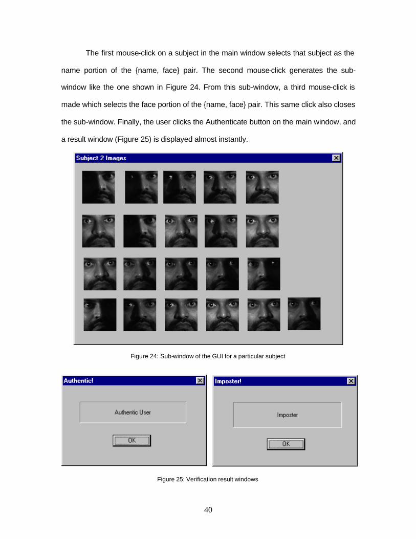
The first mouse-click on a subject in the main window selects that subject as the

name portion of the {name, face} pair. The second mouse-click generates the sub-

window like the one shown in Figure 24. From this sub-window, a third mouse-click is

made which selects the face portion of the {name, face} pair. This same click also closes

the sub-window. Finally, the user clicks the Authenticate button on the main window, and

a result window (Figure 25) is displayed almost instantly.

Figure 24: Sub-window of the GUI for a particular subject

Figure 25: Verification result windows

41

The GUI provides a friendly, easy-to-use way to demonstrate the real-time

verification stage. It also simulates (in a rough way) using an ATM.

11. CONCLUSION

We have designed and implemented a Face Verification system that has a low

probability of error in the presence of illumination variation. The system has been

implemented on a Texas Instruments C67 DSP Board, and runs in real time. We have

described how we implemented this system and have analyzed our results.

12. FUTURE WORK

Besides illumination, the two other primary types of face image variation are

expression and pose. New 18-551 groups could use our project as a starting point to

design a face verification system that is robust to these other types of variation.

13. ACKNOWLEDGEMENTS

We appreciate the suggestions made by Professor Casasent throughout the

semester. His feedback on our initial proposal and our project update presentation was

valuable and allowed us to design and implement a successful project.

42

14. REFERENCES

The references below have also been included as footnotes at the appropriate

places earlier in the document.

[1] Distortion-Invariant FOPEN Detection Filter Improvements,

Casasent, Ippolito and Verly, Proc. SPIE, vol. 3721, April 1999 conference

[2] Improving the false alarm capabilities of the maximum average correlation

height correlation filter. Alkanhal, Vijaya Kumar, Mahalanobis, Proc. Opt. Eng. 39(5), 1133-1141 (2000)

[3] The CMU Pose, Illumination, and Expression (PIE) Database ,

T. Sim and S. Baker and M. Bsat, Proceedings of the 5th International Conference on Automatic Face and Gesture Recognition, 2002

[4] Distance-classifier correlation filters for multiclass target recognition A. Mahalanobis, B.V.K. Vijaya Kumar, and S.R.F. Sims Appl. Opt. 35(17), 3127-3133 (1996) [5] Texas Instruments Website

http://www-k.ext.ti.com/sc/technical-support/tools/dsp/ftp/c67x.htm