1

Face Recognition with CTFM Sonar

Kok Kai Yoong and Phillip McKerrow School of Information Technology and Computer Science

University of Wollongong, Australia kky23@uow.edu.au, phillip@uow.edu.au

Abstract

The use of biometrics, such as iris, thumbprints, voice, face, etc, for authentication have become commonplace. In this research, we are attempting to classify human faces using CTFM (Continuously Transmitted Frequency Modulated) sonar in place of the normally used computer vision. However, for this preliminary paper, the main objectives are to find out the range relationships between human facial features and how they are represented in echoes, and to test the quality of echo features for three faces from a single orientation. The tested features are features that were effective in past research into classifying objects from ultrasonic echoes. We measure the quality of these features using a minimum Euclidean distance criterion. Actual classification of faces will be attempted at a later phase.

1. Introduction

Biometric systems are security technologies that aid in the identification of a human being. These systems measure the characteristics of a human such as thumbprints, iris print, face structure or voice pattern. In recent years, biometric solutions have become increasingly popular in public spaces and work areas due to their advantages over the traditional password approach. Passwords are not user friendly, given the fact that a combination of numbers and letters are recommended for good password protection. Easily memorized passwords are usually weak passwords. They can be lost and replication may take place. Biometric data do not have these problems. A scan of the face can easily allow access to data, which promotes user friendliness. Biometric information would never be lost. Sharing of biometric characteristics such as fingerprints also proves impossible. These facts help the public accept biometric technology, creating a need for more research work into this field.

Computer vision technology is the norm when it comes to biometric recognition systems. Images belonging to a particular person are captured and stored in a database, from where they are retrieved and compared when the same person attempts to get through the system. Although computer vision represents a logical and powerful aid for biometric recognition, there is still room for improvements in this area of research.

Nature has given us more than the sense of sight for object recognition. We can also recognize objects by hearing, tasting, etc. For mammals such as bats, whales and dolphins, perception is achieved with the sense of hearing, aided by their special ability to emit sonar energy. This method of perceiving the environment is described with the term ‘echolocation’ [Fenton and Ratcliffe, 2004]. The fields of robotics and marine engineering are other good examples of where sonar energy is used for environment mapping as well as obstacle detection.

The current research replaces vision technology for the task of face classification with CTFM (Continuously Transmitted Frequency Modulated) sonar. It can be perceived as an extension to the previous research work done on plant recognition [McKerrow and Harper, 2001] and surface roughness [McKerrow and Kristiansen, 2004] classification. The aim of this research is not about replacing computer vision as the standard for face recognition, rather, it is the first step towards exploring the possibility of complementing visual face recognition with ultrasonic sensing. A successful combination of both technologies could significantly increase the performance of new face recognition systems.

The chosen pattern classification method to perform face recognition is by using a statistical classifier developed from past research. With this approach, we hope to gain better knowledge of the interaction between sonar waves and human faces as well as extracting a set of suitable features for classification.

2

2. Face Recognition with Vision

Bledsoe first documented computerized face recognition in the 1960s. His face recognition algorithm uses a feature-based approach algorithm, where mathematical calculations were made between important facial features such as the distance between the eyes, distance between the eyes and nose, etc [Kelly, 2004]. Today, this method and other image-based algorithms are widely used by visual face recognition systems. For recognition systems, vision technology is preferred over sonar because of the simple fact that humans identify faces with their visual senses.

Current vision technology has its fair share of problems. Zhao et al. [2003] gave a complete picture of the problems faced by current visual systems. Visual systems that recognize faces using a holistic approach may be quick but the discriminant information they provide may not be rich enough to handle large databases. This problem can be solved using feature-based analysis but by using this approach, other concerns will arise such as determining how and when to use these features.

The challenge of developing a face detection technique that reports not only the presence of a face but also the accurate location of facial features under large pose and illumination variations still remains. How to model face variation under realistic settings is yet another challenge. Examples could be outdoor environments (night time, mist & fogs), natural aging, etc.

In 2002, the American Civil Liberties Union (ACLU) tested Identix’s face recognition system at the Palm Beach International Airport in Florida. The statistics released after the test showed that the system failed to identify the employees 53% of the time against the database. Another test reported by Boston’s Logan International Airport using both Identix and Viisage Technologies face recognition system failed 38% of the time. Only the Cognitec system performed better at the Sydney Airport due to better lighting control and passenger cooperation. The recent FRVT (Face recognition vendor test) conducted in year 2002 also failed to achieve a satisfactory level of performance from a total of ten participants. [Kung et al, 2005]

The above problems stated for visual face recognition justify the idea of attempting to use sonar in face recognition. Sonar may be able to solve some problems faced by visual systems. An example may be helping to detect and recognize faces in various outdoor environments (including night time, low-visibility areas). Sonar advantages over vision have also been discussed by McKerrow and Harper [1999]. These two technologies could also be integrated to form a superior hybrid face recognition system. [Kjeldsen, 2001]

3. Previous Work With Ultrasonic Sensing

Dror et al. [1995] attempted to use neural networks to show how sonar echoes can be represented and described for 3D object recognition. The major components of their system include using sonar sounds similar to bats, a neural network that can recognize objects independent of orientation and 2 highly classifiable 3D objects as targets for insonification. The echoes gathered are encoded in a time, frequency and time-frequency structure (represented by spectrograms, waveforms, power spectra and cross-correlation) before feeding into a neural network.

The performance of each representation was then observed and measured for further comparison. The best classification result came from using a time-frequency spectrogram at 97%. This enabled Dror et al. [1995] to conclude that time-frequency information gives better object recognition performance than other forms of structure representation.

However, it did not show that sonar can be used for complex object and pattern recognition such as the human face. Therefore, we have to look at sonar research involving complex pattern recognition.

Dror et al. [1996] started another sonar research project with human face recognition being part of the objective. This project was a continuation of their last project on sonar object recognition. Time-frequency spectrograms, as concluded in their previous work as the best way to represent 3D object, were used as the representation method for the human face. What they did was to build a standard data collection procedure, gather human resources, get the face echoes and encode them into spectrograms. These spectrograms were then used as training materials for the neural network. The actual performance test started after the training was done. Face echo samples not used in training the neural network were collected and used for testing.

The result in correct identification of faces was unsatisfactory. With five faces, the network was able to generalize and identify at an accuracy of 96%. An additional sixth face was added and the network performance dropped to a level of 81%. The seventh face could not be recognized at all. With these observations, they concluded that the backpropagation algorithm used by the neural network did not scale well and thus was a limitation imposed by system computational power. [Dror et al, 1996]

The present research is focused on using a statistical classifier approach to perform classification of faces. This approach involves applying the concept of modeling of face echoes which

• helps to predict what to look for in an echo (feature identification), and

• helps to understand how geometry creates the echo. This understanding provides a scientific basis for

3

defining and selecting echo features to solve the face recognition problem

Therefore, we will look at past research involving

these concepts. Mckerrow and Harper [1999, 2001] attempted plant classification research to assist with robot navigation. Using a CTFM system developed to aid blind people, they captured the echoes of 100 plant species each with their own characteristics. The echoes were then transformed into the frequency domain with an FFT (Fast Fourier Transform) and stored into data files. These data files were then read with self programmed software to extract features and recognize the different plant species. From this research, they developed a model (Acoustic Density Profile), which helps to identify a total of 19 usable features to interpret the information in echoes generated from the plant.

The plant recognition research shows that echo features can be used to classify plants, but does not give an actual classification rate. Therefore, McKerrow and Kristiansen [2004] give a detailed explanation of how 12 classes of surfaces are classified in their surface roughness classification research.

Similar to the plant recognition research, a model known as the spatial-angle-filter model was developed which is a combination of a transducer model, an acoustic reflection model and a model of surface geometry. This model allows identification of geometric features for 2 dimensional surfaces and shows the interaction of CTFM sonar with different classes of surface. A total of 12 features are identified and by employing a statistical classifier that uses the Mahalanobis distance calculation, they are able to measure the quality of each feature as well as for classification. The result shows a classification rate of 99.73% on 12 classes of surface, using a combination of 5 features.

Politis and Probert [1999, 2001] & Probert and Politis [2003] have shown us that good classification rates can be achieved by using only a few features. Using the K-nearest neighbor classifier with 8 classes of surface, Politis & Probert were able to achieve a result of 92.8% by using only one measurement and an increment to 95.1% when a second measurement was taken. By increasing the number of features from two to three and applying averaging to some surfaces, they were able to achieve classification rates near to 100%. This high level of classification results was due to using classifiers that assume Euclidean converging of the sample data.

Wen and Hinders [2005] were able to automatically distinguish 20 trees from 10 round metal poles by developing an algorithm for a sonar system strapped to a robot. A series of scans were needed to perform successful classification using a feature known as Average Asymmetry-Average Squared Euclidean Distance.

The previous work discussed here shows that previous face recognition research based on a neural network did not achieve a satisfactory result. We also understand that echo features have been successfully integrated with statistical approaches in object classifications.

4.Universal Model, Facial Features and Echoes

The face is the target object where we obtain echo data. Due to no research work in understanding how faces interact with CTFM sonar, we will explore their relationship by discussing the effects of human facial features and face geometry on face echoes in the next three sub sections.

The first step towards the aim of understanding face geometry and sonar interaction is to find a universal face model that we can base our study on. This model is suppose to be the ideal face that acts as a reference for the majority of human faces from most orientations and is minimally affected by the gender and ethnic issues. By having this universal model, we can thus focus our theoretical explanation on a single face.

The “Repose Masks” (Fig 4a) created by Marquardt Beauty Analysis [2005] suits our research requirements specified above. It is a universal face shown from both front and side view with well-defined facial features. Thus we will base our theoretical discussion on this model.

Fig 4a – Repose Frontal Mask & Repose Lateral Mask (Also referred to as

Universal Face model) [Marquardt Beauty Analysis, 2005]

4.1 Facial Feature Positioning & Orientation

The parameters of the echo largely depend on the orientation of the human face. Every one degree orientation of the face may result in very different echoes and thus for this initial research only the frontal view of the face will be examined. Sonar energy traveling towards the face will bounce off different facial features. This means that the positioning of facial features is important for the research. There is a standard natural arrangement of individual features on faces.

4

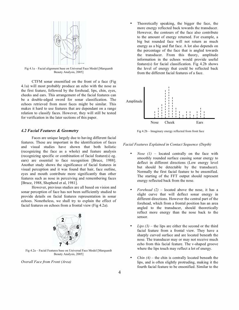
Fig 4.1a – Facial alignment base on Universal Face Model [Marquardt Beauty Analysis, 2005]

CTFM sonar ensonified on the front of a face (Fig

4.1a) will most probably produce an echo with the nose as the first feature, followed by the forehead, lips, chin, eyes, cheeks and ears. This arrangement of the facial features can be a double-edged sword for sonar classification. The echoes retrieved from most faces might be similar. This makes it hard to use features that are dependant on a range relation to classify faces. However, they will still be tested for verification in the later sections of this paper.

4.2 Facial Features & Geometry

Faces are unique largely due to having different facial features. These are important in the identification of faces and visual studies have shown that both holistic (recognizing the face as a whole) and feature analysis (recognizing specific or combination of facial feature(s) eg. ears) are essential to face recognition [Bruce, 1988]. Another study shows the significance of facial features in visual perception and it was found that hair, face outline, eyes and mouth contribute more significantly than other features such as nose in perceiving and remembering faces [Bruce, 1988, Shepherd et al, 1981].

However, previous studies are all based on vision and sonar perception of face has not been sufficiently studied to provide details on facial features representation in sonar echoes. Nonetheless, we shall try to explain the effect of facial features on echoes from a frontal view (Fig 4.2a).

Fig 4.2a – Facial Features base on Universal Face Model [Marquardt Beauty Analysis, 2005]

Overall Face from Front (Area)

• Theoretically speaking, the bigger the face, the more energy reflected back towards the transducer. However, the contours of the face also contribute to the amount of energy returned. For example, a big but rounded face will not return as much energy as a big and flat face. A lot also depends on the percentage of the face that is angled towards the transducer. From this theory, amplitude information in the echoes would provide useful feature(s) for facial classification. Fig 4.2b shows the level of energy that could be reflected back from the different facial features of a face.

Fig 4.2b – Imaginary energy reflected from front face

Facial Features Explained in Contact Sequence (Depth)

• Nose (1) – located centrally on the face with smoothly rounded surface causing sonar energy to deflect in different directions (Low energy level but should be detectable by the transducer). Normally the first facial feature to be ensonified. The starting of the FFT output should represent energy reflected back from the nose.

• Forehead (2) – located above the nose, it has a slight curve that will deflect sonar energy in different directions. However the central part of the forehead, which from a frontal position has an area angled to the transducer, should theoretically reflect more energy than the nose back to the sensor.

• Lips (3) – the lips are either the second or the third facial feature from a frontal view. They have a sharply curved surface and are located beneath the nose. The transducer may or may not receive much echo from this facial feature. The v-shaped groove where the lips touch may reflect a lot of energy.

• Chin (4) – the chin is centrally located beneath the lips, and is often slightly protruding, making it the fourth facial feature to be ensonified. Similar to the

Nose Cheek Ears

Amplitude

5

forehead, it is angled towards the transducer and should be able to deflect some energy back to the transducer.

• Cheeks (5) – the cheeks are located on the face to both sides of the nose. The areas near the nose are angled more towards the sensor, causing some sonar energy to be deflected back towards the sensor. However, the area further from the nose near the ears deflects energy away from the transducer. People with a wider face may have cheeks that are larger, hence deflecting more energy back to the transducer than people with a narrow face.

• Eye Socket (6) – the eye sockets together with the eyeballs and are located between the forehead and the nose. People with deep eye sockets may reflect more energy towards the transducer.

• Neck (7) – this is not an area that we are interested in. However, it is hard not to get some echoes back from the neck.

• Hair (8) – another area of lesser concern. However, the density of the hair will probably have an effect on the energy level returned towards the transducer. This feature needs to be further tested.

• Ears (9) – Theoretically the last facial feature to be ensonified by the sensors. They are located to the side of the face. If the range measurement corresponds to the facial depth measurement of the face, the amplitudes near the end of the FFT are likely to be energy reflected by the ears. People with protruding ears are more likely to reflect energy back to the transducer from their ears.

• Others – Possible feature that can deflect sonar energy are the teeth. During facial expression changes, the teeth might be exposed to sonar thus reflecting energy back towards the transducer.

From the above analysis, none of the facial features seem able to reflect large amounts of sonar energy back to the transducer. Therefore, we believe that the total sonar energy received by the transducer will be relatively small.

4.3 Facial Variations

Fig 4.3a Front and side facial changes due to different expressions [Marquardt Beauty Analysis, 2005]

Facial variation is another area of concern for the

present research. We have to understand the causes of facial variation in order to perform quality data collection. Facial variations can occur between people or individuals. Studies by Marquardt Beauty Analysis [2005] have shown that these variations are caused by three major factors and can be categorized as age, gender and race. Race and gender can cause variations between people, while aging affects all individuals. Also, facial variations can occur simply by smiling, talking or wearing ornaments. Therefore, in this initial stage of testing, facial variations will not be taken into account.

4.4 Face Acoustic Model

This section has provided an insight into how sonar interacts with the Universal Face Model from a front view, which would form the basis for developing a Face Acoustic Model. In summary, we have discussed factors that directly influence echo data. They include face orientation, positioning (Section 4.1), facial features and geometry (Section 4.2) from a frontal view. We have also discussed facial variations. These issues are crucial to the quality of the echo data collected, and therefore must be understood in order to make plans for the later phases of the research.

5. Features and Quality Measurement

Features are characteristics of echoes that can potentially be used as a mean of classification. The results from past research using features are encouraging (Section 3). However, features have varied classification abilities. Certain features perform better than the others, but no single feature can be used to classify a large number of objects. For this reason, a combination of features is needed in order to gain better classification. The quality of each feature and overall classification ability will be measured to explain which features perform better in this research.

5.1 Inherited Features

The demodulated echo signal is transformed into frequency space with an FFT (Fast-Fourier Tranform). From the FFT of the echo, there is a need to select the region of interest to produce a set of range bins that contain only echoes from the face. This is a process known as windowing. It helps to discard data not belonging to the face and converts absolute range data into relative range data.

The windowed data is used in feature extraction. In the previous plant and surface roughness classification, a

6

total of 31 features were used. Out of these 31 features, 15 have been chosen for this initial testing. These features together with their origin are summarized in table 5.1a and explained below.

Origin Features

Plants

Length of density profile Sum of density profile

Front to peak dist Peak 1 Amplitude

Freq 75 acoustic area Threshold 1 - 9

Roughness Average acoustic area

Table 5.1a Length of Acoustic Density Profile This is the distance between the first and last range line in the windowed echo. In geometrical terms, it represents the depth of the face. The measurement of facial depth differs between people. In practice, this depth will probably be the distance from the nose to the edge of the ears. Sum Of Density Profile The sum of the amplitudes of the first to the last range line is the total energy reflected from the face in the direction of the transducer. It is equivalent to the area of the face in the Face Acoustic Model. The amplitude of the echo at each range is proportional to the acoustic area at the same range. Therefore, by summing up the amplitudes of the bins, we will calculate the total acoustic area of the face. This feature is highly applicable to human faces as energy reflected from different people should vary between people. For example, a person with a wider face will probably reflect more energy back to the transducer thus resulting in higher acoustic area. Front to Peak Distance This will give us the distance from the nose to the feature that reflects the most energy – possibly the cheeks or the eye socket. Peak 1Amplitude This will give us the amount of energy reflected from the facial feature that reflects the most energy. 75% Acoustic Area This feature calculates the range from the first detected reflecting surface to the cell that accumulates 75% of the total density profile acoustic area. Threshold 1 - 9 The 9 threshold values are calculated from the transducer noise level. For each of the threshold levels, bins with lesser

values are filtered and the remaining bins are summed to get new values. Average Acoustic Area A feature from the roughness research is the average acoustic area of the transformed echo. It is calculated by averaging the total acoustic area over the count of range bins.

5.2 Feature Quality

Different feature are measured in different units. In order to compare the quality of features, the extracted feature values are first converted into a common scale (Units of Standard Deviation). Measuring of the classification quality of features is discussed in this section.

The extracted feature values are combined into a feature vector (v) with n features. The feature vector v represents a point in the n-dimensional feature space V. Every point in V corresponds to one collection of the measurement data. The set of feature with vectors of feature data that cluster together and have minimum overlap with clusters for other faces will be quality features.

To identify a face, a reference vector is calculated with the cluster of echoes for the same face. A probability density function is used to model the measured features for each face. Vector v will have a mean vector µ, a standard deviation vector σ and a covariance matrix K.

There are two ways of measuring feature quality, the first is by calculating the Euclidean distance between reference vectors and to use those that give larger distances. The Euclidean distance represents the physical distance between mean vectors in a 2D feature space. It is a linear classifier that does not take into account the standard deviations of features. The standard deviation measures that spread of the cluster and hence gives a measure of the quality of a feature.

A second way of getting feature quality and classification is with the Mahalanobis distance. The Mahalanobis distance is also a linear classifier that takes into account the standard deviations and hence is a better way of measuring the quality of features. It includes the covariance matrix K and gives a measure in units of standard deviations unlike the Euclidean distance, which is in physical distance. However, the Mahalanobis distance can be calculated with Euclidean distance when the feature values are normalized by dividing the mean by the standard deviation. [McKerrow and Kristiansen, 2004]

In this section, we have given a brief theoretical explanation of the process of measuring feature quality. In the next 2 sections, we will talk about the design of our experiment, as well as some preliminary test results.

7

6. Experiment Design

The initial experiment consists of the following components

Fig 6a – transducer

• 1 transducer for transmitting and receiving CTFM

sonar and echo • 1 stand for holding the transducer

• 1 Macintosh for running classification software • The classification software written in Labview7.1 • 3 test subjects (Include 2 faces modeled from

different material and a human face Fig 6b-6d) • 1 stool for test subject to sit on

Fig 6b – Cardboard Fig 6c – Polystyrene Fig 6d – Human Face

The setup for this preliminary test is as shown in Fig 6e. Setting up the data collection process requires knowledge of the target distance from the transducer as well as the distance of the face from ground level. The distance of target from transducer is determined by the physical measurement of the transducer. Based on a calculation derived from McKerrow [1991], to have the full face within the field of audition, the transducer has to be placed more than 1000mm from the target.

Fig 6e – Test Setup The following data is captured for each face and stored in a file.

• Metadata of test subjects (eg. date of echo captured, name of person, etc…)

• 64 echoes per test subject from a frontal view

The following are requirements that have to be followed when collecting echoes.

• Distance to transducer is set at 1000 cm • Distance from ground is set at 1124mm (position

of human nose) • Test subject is required to remain still within the

period of echo capture • Test will be conducted in a space free of

interference • Standard software settings

The purpose of this preliminary test is to find out

• The noise level emitted from the transducer • The distance of test subject as shown in the FFT • mm per bin measurement • How facial features are represented in the FFT

o Using a cardboard face model o Using a polystyrene face model o Using an actual human face

• The quality of proven features from past research on current test subjects

7. Preliminary Results

Exp 1 – Understanding transducer noise level This test is to find out the value of background noises,

where does it occur in the FFT, and thus exclude it during windowing.

Fig 7a – FFT showing noise level in transducer Result:

The result shows that noises average at a value of 3.8 Nanovolts between the range of 0 to 500 FFT bins. This result meant that the transducer captures a fairly low amount of noise from the environment. The reading we got from measuring transducer noise level is a good threshold value for filtering noise and thus aids in detecting echoes from faces. In the roughness classification paper written by McKerrow and Kristiansen (2005), they suggested setting a threshold of Mean + 5 Standard Deviations which is (µ + 5σ)

8

in mathematical representation. From this calculation, we got a threshold value of about 25n (Nanovolts). Exp 2 – Windowing test subject FFT and measuring mm/bin

We need to know where the reflected energy of the test subject is detected in the FFT. During windowing, we can thus focus on getting the correct echoes from the test subject. In order to get a signal thus indicating the presence of an object, we opt to place an object (a ball) at the distance of 905mm. The mm per bin value, also referred to as the resolution of the transducer, can thus be calculated by dividing the fixed distance of 905mm by the measured FFT bin number.

Fig 7b – test subject shown in the FFT

Result: This result shows that an object (the ball) has been

detected at bin 233 and 234. Therefore, our windowing shall only include bins that are higher than bin 220. Those FFT before bin 220 will be discarded. The mm/bin is thus calculated by dividing 905 with 234, which gives a measurement of 3.867. Exp 3 – Capturing values from cardboard model (Fig 6b)

The cardboard model is a simple face geometry model with actual face measurements. The flat surfaces are designed to reflect more energy back to the transducer so as to find out the range relationship within the echo of different facial features.

Fig 7c – Windowed FFT Transformed echo for cardboard model

Result:

Fig 7c shows that the cardboard model had been detected at bin 298 and ends at bin 319. From the experiment 2, we know that the mm/bin value is 3.867. Therefore, a total of 21 bins (319 -298) is equivalent to a measurement of 81.2mm (3.867 x 21) depth of the face. The cardboard model has a total depth of 75mm. This represents a difference of less than 2 bins (6.2mm), which is not significant in terms of sonar.

Using the universal face model (Fig 4a) as a guide, the bin numbers from 298 – 303 represents the reflected energy from the nose, lips and forehead. Bins 303 - 307 represent the forehead and the cheek of the face, while the remaining bins represent the side face and ears of the model. Some surfaces of the cardboard model are not angled towards the transducer (nose, lips, chin and ears), which might explain the very little energy reflected towards the transducer for these facial features. Therefore from the acoustic profile of the cardboard model, we observe that the cheek area returns a much more significant amount of energy as shown in Fig 7c.

From this reading, we conclude that the model has partially fulfilled its role in representing the echoes from all the facial features, since not much energy from the ears was captured and we cannot model the effects of hair and teeth on echoes. Exp 4 - Capturing values from polystyrene face model

The polystyrene face model closely resembles the shape of a human face. Compared to a real human, this model does not move and does not have any hair. Therefore, this model is thought to be the ‘perfect’ model for echo data analysis. Since it doesn’t move, we can try to capture its echoes from all angles for further experiments. The flaw with this model is it doesn’t have ears. Also since the reflective qualities of human skin are different to polystyrene, the analysis results may not be applicable to humans. However, in this initial experiment, we have decided to include this model.

Fig 7d – transducer transmitting and receiving echo from polystyrene face

9

Fig 7e - Windowed FFT Transformed echo for Polystyrene Result:

With this polystyrene model, we started to get a reading at bin 259 (end at bin 288). The signal received is much lower in amplitude compared to the cardboard model. We apply our knowledge of the human face on the polystyrene model and assume that the first bin (259) belongs to the nose. This is followed by energy reflected from the lips and forehead, which is not really the amount of energy we anticipated. The rest of the readings are also not what we expected (notice the sudden increase and decrease in bin amplitude in Fig 7e). Therefore, we cannot relate the reflected energy to the model’s facial features. Exp 5 - Capturing values from human face

This research is ultimately about human face recognition/classification. Therefore, the final test subject uses a real human face for experiment.

Fig 7f - Windowed FFT Transformed echo for human face Result:

Echoes from a human face started at about bin 253. This represents reflected energy from the nose. At bin 259, the first peak is reached, which using the universal model as a reference, represents the forehead. Bin 264 – 267 has high-reflected energy which represents energy from the cheek and eye socket. After bin 267, less energy is received

and it is probably energy reflected from the side cheek. At bin 290, the amplitude rises again which is energy reflected from the ears. The FFT transformed echo of the human face is similar to the imaginary echoes shown in Fig 4.2b. Summary of Experiments 3 - 5:

We can see that the cardboard model has much higher peak amplitude compared to the human face and polystyrene model. This is due to the flat surface design on all the individual facial feature of the face model. We can also map the cardboard facial features to the bins in the mean diagram. However, from the mean diagram of the polystyrene model, it is hard to identify the relationship between its facial features and the FFT bins. For the test done on the human face, we successfully mapped the FFT bins to the facial features. The mappings of facial features to FFT bins represent the first step towards classification of faces. Exp 6 – Measuring Feature Quality

In our final experiment, we sought to measure the quality of the features in table 5.1a using the method described in section 5.2. Once the distances for each feature are found, we can measure feature quality by using either minimum distance or count of distances < threshold.

Rank Feature Name Minimum Distance (σ)

1 Average Acoustic Area 1.3774

2 Threshold 1 1.12177

3 Threshold 2 1.09829

4 Threshold 4 1.09655

5 Threshold 3 1.09255

6 Threshold 6 1.07133

7 Threshold 5 1.04765

8 Threshold 7 1.00089

9 Sum of Face Profile 0.989914

10 Threshold 8 0.884734

11 Length of Face Profile 0.884556

12 Threshold 9 0.848657

13 Distance to Peak 1 0.567084

14 Peak 1 Amplitude 0.32627

15 Length of Profile to 75% Acoustic Area 0.0505156

Table 7a – Measuring Feature Quality using Minimum Distances

Table 7a shows features arranged in descending order of minimum Mahalanobis distance (Euclidean distance of

10

normalized vectors) in 1D space. This also represents the quality of the features in face classification. From the table, feature “Average Acoustic Area” is the best feature while ”Length of Profile to 75% Acoustic Area” is the worst feature to classify the 3 test subjects.

Another way of measuring feature quality is to count the distances for each feature that are less than a certain threshold, which we set at 1σ. The lower the count, the better the feature quality is. However, the 3 test subjects used in this preliminary paper will only result in a maximum of 3 distances between all test subjects, thus we will not measure feature quality using this criterion.

8. Classification Result

The minimum distances (classification) of features we have in table 7a are measured in units of standard deviation. Referring back to table 7a, any of the first 8 features are able to classify our test subjects at a rate of 68.26% (1σ). To increase the minimum distances to at least 2σand hence a classification rate of 95.45%, the top 3 features are needed. To further increase all the minimum distances to over 3σ (99.73%), we require a combination of the top 7 features. To achieve a classification quality of 4σ (99.9937%), we need to use all 15 features and 5σis not achievable unless new quality features are found.

9. Conclusion

In this research, we made an attempt to describe the interaction between human faces and sonar energy in Section 4. We also conducted experiments in Section 7 based on the explanation given in Section 5 and test design described in Section 6. Experiments 3 and 5 successfully confirms what we have described in Section 4, while experiment 4 may need further testing. In the final experiment, we have shown the quality of each feature for classification using the minimum distance criterion. Using Table 7a, we have also successfully classified the 3 test subjects with reference to the Gaussian distribution. However, this initial research is based on 3 test subjects of different nature, which means that further testing on more test subjects of the same nature (human face) are needed to verify the results we have got here.

Relevant References Bruce V. 1988. ‘Recognizing faces’. Lawrence Erlbaum

Associates, London, U.K. Dror IE., Zagaeski M. and Moss CF. 1995. ‘Three-Dimensional

Target Recognition Via Sonar: A Neural Network Model’. Neural Networks. Vol. 8, no. 1, pp. 149-160.

Dror IE., Florer FL., Rios D. and Zagaeski M. 1996. ‘Using artificial bat sonar neural networks for complex pattern recognition: Recognizing faces and the speed of a moving target’. Biological Cybernetics. Vol. 74, pp. 331-338.

Fenton B. and Ratcliffe J. 2004. ‘Animal Behavior: On Bat Echolocation’ [Online]. Available URL: http://scienceweek.com/2005/sw050325-3.htm. [Accessed: 20 Mar 2005]

Kelly G. 2004. ‘The Past Perfect Promise of Facial Recognition Technology’ [Online]. ACDIS Occasional Paper. Available URL : http://www.acdis.uiuc.edu/Research/OPs/Gates/contents/part2.html. (Viewed: 20 Mar 2005)

Kjeldsen R. and Hartman J. 2001. ‘Design Issues for Vision-based Computer Interaction Systems’. ACM International Conference Proceeding Series. pp. 1-8.

Kung SY., Mak MW and Lin SH. 2005, ‘Biometric Authentication By Face’, Biometric Authentication. Upper Saddle River, NJ, Prentice Hall, pp. 241-276.

Marquardt Beauty Analysis. 2005. ‘Normal Face Variations- From The Mask’ [Online]. Available URL: http://www.beautyanalysis.com/index2_mba.htm [Accessed 15 April 2005]

McKerrow, P.J. 1991, reprinted 1993, 1995 and 1998(twice). Introduction to Robotics , Addison-Wesley, Electronic Systems Engineering Series, Wokingham, ISBN 0 201 18240 8, 811 pages. English Sales: 11,639 copies sold.

McKerrow P. and Harper N. 1999. ‘Recognizing leafy plants with in-air sonar’. Sens.Rev. Vol. 19, no. 3, pp. 202-206.

McKerrow P. and Harper N. 2001. ‘Plant acoustic density profile model of CTFM ultrasonic sensing’. IEEE Sensors Journal. Vol. 1, no. 4, pp. 245-255. Available e-mail: phillip@uow.edu.au

McKerrow P. and Kristiansen BJ. 2004. ‘Measurement of Roughness with CTFM Ultrasonic Sensing’. Submitted to IEEE Sensors Journal

Politis Z. and Probert PJ. 1999. ‘Modelling and classification of rough surfaces using CTFM sonar imaging’. Conference on Robotics and automation. pp. 2988-2993.

Politis Z. and Probert PJ. 2001. ‘Classification of textured surfaces for robot navigation using continuous transmission frequency-modulated sonar signatures’. The International Journal of Robotics Research. Vol. 20, no. 2, pp. 107-128.

Probert PJ. and Politis Z. 2003. ‘Sonar for recognizing the texture or pathways’. University of Oxford, conference review.

Schwarzer G. and Leder H. 2003. ‘The development of face processing’. Hogrefe & Huber, Toronto.

Shepherd JW., Davies GM. and Ellis HD. 1981. ‘Studies of cue saliency’. In Perceiving and Remembering Faces. Davies GM. Ellis HD. and Shepherd JW. Eds. Academic Press, London, U.K.

Wen G. and Hinders HK. 2005. ‘Mobile Robot Sonar Interpretation Algorithm for Distinguishing Trees from Poles’. (Unpublish)

Zhao W., Chellappa R., Phillips PJ. and Rosenfeld A. 2003. ‘Face Recognition: A Literature Survey’. ACM Computing Surveys (CSUR). Vol. 34, no. 4, pp. 399-458.