FACE RECOGNITION

USING EIGENFACES AND NEURAL NETWORKS

A THESIS SUBMITTED TO

THE GRADUATE SCHOOL OF NATURAL AND APPLIED SCIENCES

OF

THE MIDDLE EAST TECHNICAL UNIVERSITY

BY

VOLKAN AKALIN

IN PARTIAL FULFILMENT OF THE REQUIREMENTS FOR THE DEGREE OF

MASTER OF SCIENCE

IN THE DEPARTMENT OF ELECTRICAL AND ELECTRONICS ENGINEERING

DECEMBER 2003

Approval of the Graduate School of Natural and Applied Sciences

__________________

Prof. Dr. Canan ÖZGEN

Director

I certify that this thesis satisfies all the requirements as a thesis for the degree of

Master of Science.

__________________

Prof. Dr. Mübeccel DEMİREKLER

Head of Department

This is to certify that we have read this thesis and that in our opinion it is fully

adequate, in scope and quality, as a thesis for the degree of Master of Science.

__________________

Prof. Dr. Mete SEVERCAN

Supervisor

Examining Committee Members

Prof. Dr. Gönül Turhan SAYAN __________________

Prof. Dr. Mete SEVERCAN __________________

Assoc. Prof. Dr. Gözde Bozdağı AKAR __________________

Assoc. Prof. Dr. A.Aydın ALATAN __________________

Dr. Uğur Murat LELOĞLU __________________

ii

ABSTRACT

FACE RECOGNITION USING EIGENFACES

AND NEURAL NETWORKS

AKALIN, Volkan

M.S., The Department of Electrical and Electronics Engineering

Supervisor: Prof. Dr. Mete SEVERCAN

December 2003, 91 Pages

A face authentication system based on principal component analysis and

neural networks is developed in this thesis. The system consists of three stages;

preprocessing, principal component analysis, and recognition. In preprocessing

stage, normalization illumination, and head orientation were done. Principal

component analysis is applied to find the aspects of face which are important for

identification. Eigenvectors and eigenfaces are calculated from the initial face

image set. New faces are projected onto the space expanded by eigenfaces and

represented by weighted sum of the eigenfaces. These weights are used to identify

the faces. Neural network is used to create the face database and recognize and

authenticate the face by using these weights. In this work, a separate network was

build for each person. The input face is projected onto the eigenface space first and

new descriptor is obtained. The new descriptor is used as input to each person’s

network, trained earlier. The one with maximum output is selected and reported as

iii

the host if it passes predefined recognition threshold. The algorithms that have been

developed are tested on ORL, Yale and Feret Face Databases.

Keywords: Face recognition, Face authentication, Principal component analysis,

Neural network, Eigenvector, Eigenface

iv

ÖZ

ÖZYÜZLER VE YAPAY SİNİR AĞLARI KULLANARAK

YÜZ TANIMA

AKALIN, Volkan

Yüksek Lisans, Elektrik ve Elektronik Mühendisliği Bölümü

Tez Yöneticisi: Prof. Dr. Mete SEVERCAN

Aralık 2003, 91 Sayfa

Bu tezde, ana bileşen analizi ve yapay sinir ağlarına dayanan bir yüz tanıma

sistemi geliştirilmiştir. Sistem üç aşamadan oluşmaktadır; önişlem, ana bileşen

analizi, ve tanıma. Önişlem aşamasında, parlaklık dengelenmesi ve baş ayarlanması

yapılmıştır. Yüz tanıma için çok önemli olan yüz görünüşlerinin bulunması için ana

bileşen analizi uygulanmıştır. Başlangıç eğitim setinden özvektörler ve özyüzler

hesaplanmıştır. Yüzler, özyüzler ile geliştirilmiş uzaya yansıtılmış ve özyüzlerin

ağırlıklı toplamları ile ifade edilmişlerdir. Bu ağırlıklar yüzleri ayırt etmek için

kullanılacaktır. Bu ağırlıkları kullanarak, yüz veritabanını oluşturmak ve yüzleri

tanımak için yapay sinir ağları kullanılmıştır. Bu çalışmada, her bir kişi için ayrı bir

yapay sinir ağı kullanılmıştır. Verilen yüz ilk olarak özyüz uzayına yansıtılarak yeni

tanımlayıcıları elde edilir. Bu yeni tanımlayıcılar daha önce eğitilmiş ağlara giriş

olarak kullanılır ve her bir kişinin ağına uygulanır. En yüksek sonucu veren ağ eğer

daha önce tanımlanmış eşik değerinin üzerindeyse seçilir ve bu ağa sahip kişi

v

aranan kişi olarak belirtilir. Geliştirilen bu algoritmalar, ORL, Yale ve Feret yüz

veritabanları üzerinde tets edilmiştir.

Anahtar Sözcükler : Yüz tanıma, Yüz doğrulama, Ana bileşen analizi, Yapay Sinir

ağı, Özvektör, Özyüz

vi

ACKNOWLEDGEMENTS

I would like to thank my supervisor, Prof Dr. Mete Severcan, for his supervision

and constructive critics in the development of this thesis. I would also express my

great gratitude to my family for their continuous support and great love. Special

thanks to Sertan Aygün, Baykal Yıldırım, and Cem Ciğdemoğlu for their great

friendships. Finally, I would like to thank to my company Aselsan and my boss

Özcan Kahramangil for their support and sensitivity in this study.

vii

TABLE OF CONTENTS

ABSTRACT..............................................................................................................iii

ÖZ............................................................................................................................. v

ACKNOWLEDGEMENTS......................................................................................vii

TABLE OF CONTENTS........................................................................................viii

LIST OF TABLES....................................................................................................xi

LIST OF FIGURES.................................................................................................xiii

CHAPTER

1. .................................................................................................. 1INTRODUCTION

1.1. Human Recognition ........................................................................................ 3

1.2. Eigenfaces for Recognition ............................................................................. 5

1.3. Thesis Organization ........................................................................................ 6

2. ................................................. 7BASIC CONCEPTS OF FACE RECOGNITION

2.1. Introduction ..................................................................................................... 7

2.1.1. Background and Related Work ................................................................ 7

2.1.2. Outline of a Typical Face Recognition System ....................................... 9

2.1.2.1. The acquisition module. .................................................................... 9

2.1.2.2. The pre-processing module. ............................................................ 10

2.1.2.3. The feature extraction module. ....................................................... 11

2.1.2.4. The classification module. .............................................................. 12

2.1.2.5. Training set...................................................................................... 12

2.1.2.6. Face library or face database........................................................... 12

2.1.3. Problems that May Occur During Face Recognition ............................. 12

2.1.3.1. Scale invariance. ............................................................................. 12

2.1.3.2. Shift invariance. .............................................................................. 13

viii

02.1.3.3. Illumination invariance. ................................................................ 13

2.1.3.4 Emotional expression and detail invariance..................................... 13

2.1.3.5. Noise invariance.............................................................................. 13

2.1.4. Feature Based Face Recognition............................................................ 14

2.1.4.1. Introduction ..................................................................................... 14

2.2.4.1.1. Deformable template model. .................................................... 15

2.2.4.1.2. Active contour model (Snake). ................................................ 15

2.1.4.2. Effective Feature Selection ............................................................. 16

2.1.4.2.1. First-order features values........................................................ 16

2.1.4.2.2. Second-order features values. .................................................. 16

2.1.4.2.3 Higher-order feature values....................................................... 17

2.1.4.3. Feature Extraction Using the Deformable Templates ..................... 20

2.1.4.3.1. Eye Template ........................................................................... 20

2.1.4.3.2. Mouth Template ....................................................................... 22

2.1.4.4. Feature Extraction Using the Active Contour................................. 23

2.1.4.4.1. The Modified Active Contour Model ...................................... 24

2.1.4.4.2. Boundary Extraction of a Face................................................. 26

2.1.5. Face Recognition Based on Principal Component Analysis.................. 28

3. ................................................. 29FACE RECOGNITION USING EIGENFACES

3.1. Introduction ................................................................................................... 29

3.2. Calculation of Eigenfaces ............................................................................. 34

3.3. Using Eigenfaces to Classify a Face Image .................................................. 38

3.4. Rebuilding a Face Image with Eigenfaces .................................................... 39

3.5. Usage of Neural Networks for Recognition:................................................. 40

3.5.1. Introduction............................................................................................ 40

3.5.2. Recurrent Neural Networks: .................................................................. 42

3.5.3. Feedforward Neural Networks:.............................................................. 43

3.5.4. Training and Simulation of Neural Networks for Recognition.............. 44

3.6. Summary of the Eigenface Recognition Procedure ...................................... 46

3.7. Comparison of the Eigenfaces Approach to Feature Based Face .....................

Recognition .................................................................................................. 47

ix

3.7.1. Speed and simplicity: ............................................................................. 47

3.7.2. Learning capability: ............................................................................... 47

3.7.3. Face background: ................................................................................... 48

3.7.4. Scale and orientation:............................................................................. 48

3.7.5. Presence of small details: ....................................................................... 48

4. RESULTS ............................................................................................................ 50

4.1. Test Results for the Olivetti and Oracle Research Laboratory (ORL) Face

Database ........................................................................................................ 51

4.2. Test Results for the Olivetti and Oracle Research Laboratory (ORL) Face

Database with Eye Extraction ....................................................................... 56

4.3. Test Results for Yale Face Database............................................................. 60

4.4. Test Results for the Yale Face Database with Eye Extraction...................... 65

4.5. Test Results for FERET Face Database ....................................................... 69

4.5.1. Preprocessing Stage ............................................................................. 76

4.6. Results for the FERET Face Database with Eye Extraction ......................... 81

5. CONCLUSION.................................................................................................... 83

REFERENCES......................................................................................................... 88

x

LIST OF TABLES

TABLE

2.1 First-order features 18

2.2 Second-order features 19

2.3 Features related to nose, if nose is noticable 19

4.1 Recognition Rate using different Number of Training and Test Images,

and w/wo Histogram Equalization 54

4.2 Recognition Rate using different Number of Eigen Faces and neurons

in Hidden Layer 55

4.3 Recognition Rate with Neural Networks different choices 56

4.4 Recognition Rate using different Number of Training and Test Images 58

4.5 Recognition Rate using different Number of Eigen Faces and neurons

in Hidden Layer 59

4.6 Recognition Rate with Neural Networks different choices 60

4.7 Recognition Rate using different Number of Training and Test Images

and with and without Histogram Equalization 63

4.8 Recognition Rate using different Number of Eigen Faces and neurons

in Hidden Layer 64

4.9 Recognition Rate with Neural Networks different choices 65

4.10 Recognition Rate using different Number of Training and Test Image 67

4.11 Recognition Rate using different Number of Eigen Faces and neurons

in Hidden Layer 68

4.12 Recognition Rate with Neural Networks different choices 69

4.13 Explanation of Naming Convention 71

4.14 The Gallery and Probe Sets used in the standard FERET test in

September 1996. 74

4.15 Feret Face Database Test Result 80

xi

4.16 Feret Face Database Tets Results with Eye Extraction 82

5.1 Performance results for ORL Face Database 85

5.2 Performance results for Yale Database 85

5.3 Performance results for Feret Face Database 87

xii

LIST OF FIGURES

FIGURE

2.1 Outline of a typical face recognition system 9

2.2 (a) Original face image 14

(b) Scale variance 14

(c) Orientation variance 14

(d) Illumination variance 14

(e) Presence of details 14

3.1 Sample Faces 30

3.2 Average face of the Sample Faces 31

3.3 Eigen Faces of the Sample Faces 31

3.4 Eigenvalues corresponding to eigenfaces 32

3.5 Reconstruction of First Image with the number of Eigenfaces. 33

3.6 Artificial Neuron 40

3.7 Recurrent Neural Networks 42

3.8 Feedforward Neural Networks 43

3.9 Training of Neural Networks 45

3.10 Simulation of Neural Networks for Recognition 46

4.1 ORL Face Database 52

4.2 Mean face for ORL Face Database 53

4.3 The eigen values for ORL Face Database 53

4.4 The top 30 eigen faces for the ORL Face Database 53

4.5 The eye extraction 57

4.6 The mean eye 57

4.7 The top 30 Eigeneyes 57

4.8 YALE Face Database 61

4.9 Mean face for YALE Face Database 62

xiii

4.10 The eigen values for ORL Face Database 62

4.11 The top 30 eigen faces for the YALE Face Database 62

4.12 Eye Extraction 66

4.13 The YALE Face Database Mean Eye 66

4.14 The YALE Face Database Top 30 Eigeneyes 66

4.15 Sample Faces 75

4.16 Sample Face with given coordinates 76

4.17 Preprocessing Stage Block Diagram 77

4.18 Preprocessing Stage 78

4.19 Tilt Compensation 78

4.20 Cropping of Face Region 79

4.21 The histogram of an image before (up) and after (down) the histogram

equalization. 79

4.22 The mask used for background removal 80

4.23 Eye Extraction 81

4.24 Cropping of Eye Region 81

xiv

CHAPTER 1

INTRODUCTION

The face is our primary focus of attention in social intercourse, playing a major

role in conveying identity and emotion. Although the ability to infer intelligence or

character from facial appearance is suspect, the human ability to recognize faces is

remarkable. We can recognize thousands of faces learned throughout our lifetime

and identify familiar faces at a glance even after years of separation. This skill is

quite robust, despite large changes in the visual stimulus due to viewing conditions,

expression, aging, and distractions such as glasses, beards or changes in hair style.

Face recognition has become an important issue in many applications such as

security systems, credit card verification and criminal identification. For example,

the ability to model a particular face and distinguish it from a large number of

stored face models would make it possible to vastly improve criminal identification.

Even the ability to merely detect faces, as opposed to recognizing them, can be

important. Detecting faces in photographs for automating color film development

can be very useful, since the effect of many enhancement and noise reduction

techniques depends on the image content.

A formal method of classifying faces was first proposed by Francis Galton in

1888 [1, 2]. During the 1980’s work on face recognition remained largely dormant.

Since the 1990’s, the research interest in face recognition has grown significantly as

a result of the following facts:

1. The increase in emphasis on civilian/commercial research projects,

1

2. The re-emergence of neural network classifiers with emphasis on real

time computation and adaptation, ,

3. The availability of real time hardware,

4. The increasing need for surveillance related applications due to drug

trafficking, terrorist activities, etc.

Although it is clear that people are good at face recognition, it is not at all

obvious how faces are encoded or decoded by the human brain. Developing a

computational model of face recognition is quite difficult, because faces are

complex, multi-dimensional visual stimuli. Therefore, face recognition is a very

high level computer vision task, in which many early vision techniques can be

involved.

The first step of human face identification is to extract the relevant features

from facial images. Research in the field primarily intends to generate sufficiently

reasonable familiarities of human faces so that another human can correctly identify

the face. The question naturally arises as to how well facial features can be

quantized. If such a quantization if possible then a computer should be capable of

recognizing a face given a set of features. Investigations by numerous researchers

[3, 4, 5] over the past several years have indicated that certain facial characteristics

are used by human beings to identify faces.

There are three major research groups which propose three different approaches

to the face recognition problem. The largest group [6, 7, 8] has dealt with facial

characteristics which are used by human beings in recognizing individual faces.

The second group [9, 10, 11, 12, 13] performs human face identification based on

feature vectors extracted from profile silhouettes. The third group [14, 15] uses

feature vectors extracted from a frontal view of the face. Although there are three

different approaches to the face recognition problem, there are two basic methods

from which these three different approaches arise.

The first method is based on the information theory concepts, in other words,

on the principal component analysis methods. In this approach, the most relevant

information that best describes a face is derived from the entire face image. Based

2

on the Karhunen-Loeve expansion in pattern recognition, M. Kirby and L. Sirovich

have shown that [6, 7] any particular face could be economically represented in

terms of a best coordinate system that they termed "eigenfaces". These are the

eigenfunctions of the averaged covariance of the ensemble of faces. Later, M. Turk

and A. Pentland have proposed a face recognition method [16] based on the

eigenfaces approach.

The second method is based on extracting feature vectors from the basic parts of

a face such as eyes, nose, mouth, and chin. In this method, with the help of

deformable templates and extensive mathematics, key information from the basic

parts of a face is gathered and then converted into a feature vector. L. Yullie and S.

Cohen [17] played a great role in adapting deformable templates to contour

extraction of face images.

1.1. Human Recognition

Within today’s environment of increased importance of security and

organization, identification and authentication methods have developed into a key

technology in various areas: entrance control in buildings; access control for

computers in general or for automatic teller machines in particular; day-to-day

affairs like withdrawing money from a bank account or dealing with the post office;

or in the prominent field of criminal investigation. Such requirement for reliable

personal identification in computerized access control has resulted in an increased

interest in biometrics.

Biometric identification is the technique of automatically identifying or

verifying an individual by a physical characteristic or personal trait. The term

“automatically” means the biometric identification system must identify or verify a

human characteristic or trait quickly with little or no intervention from the user.

Biometric technology was developed for use in high-level security systems and law

enforcement markets. The key element of biometric technology is its ability to

identify a human being and enforce security [18].

Biometric characteristics and traits are divided into behavioral or physical

categories. Behavioral biometrics encompasses such behaviors as signature and

3

typing rhythms. Physical biometric systems use the eye, finger, hand, voice, and

face, for identification.

A biometric-based system was developed by Recognition Systems Inc.,

Campbell, California, as reported by Sidlauskas [19]. The system was called ID3D

Handkey and used the three dimensional shape of a person’s hand to distinguish

people. The side and top view of a hand positioned in a controlled capture box were

used to generate a set of geometric features. Capturing takes less than two seconds

and the data could be stored efficiently in a 9-byte feature vector. This system could

store up to 20000 different hands.

Another well-known biometric measure is that of fingerprints. Various

institutions around the world have carried out research in the field. Fingerprint

systems are unobtrusive and relatively cheap to buy. They are used in banks and to

control entrance to restricted access areas. Fowler [20] has produced a short

summary of the available systems.

Fingerprints are unique to each human being. It has been observed that the

iris of the eye, like fingerprints, displays patterns and textures unique to each

human and that it remains stable over decades of life as detailed by Siedlarz [21].

Daugman designed a robust pattern recognition method based on 2-D Gabor

transforms to classify human irises.

Speech recognition is also offers one of the most natural and less obtrusive

biometric measures, where a user is identified through his or her spoken words.

AT&T has produced a prototype that stores a person’s voice on a memory card,

details of which are described by Mandelbaum [22].

While appropriate for bank transactions and entry into secure areas, such

technologies have the disadvantage that they are intrusive both physically and

socially. They require the user to position their body relative to the sensor, and then

pause for a second to declare himself or herself. This pause and declare interaction

is unlikely to change because of the fine-grain spatial sensing required. Moreover,

since people can not recognize people using this sort of data, these types of

identification do not have a place in normal human interactions and social

structures.

4

While the pause and present interaction perception are useful in high

security applications, they are exactly the opposite of what is required when

building a store that recognizing its best customers, or an information kiosk that

remembers you, or a house that knows the people who live there.

A face recognition system would allow user to be identified by simply

walking past a surveillance camera. Human beings often recognize one another by

unique facial characteristics. One of the newest biometric technologies, automatic

facial recognition, is based on this phenomenon. Facial recognition is the most

successful form of human surveillance. Facial recognition technology, is being used

to improve human efficiency when recognizing faces, is one of the fastest growing

fields in the biometric industry. Interest in facial recognition is being fueled by the

availability and low cost of video hardware, the ever-increasing number of video

cameras being placed in the workspace, and the noninvasive aspect of facial

recognition systems.

Although facial recognition is still in the research and development phase,

several commercial systems are currently available and research organizations, such

as Harvard University and the MIT Media Lab, are working on the development of

more accurate and reliable systems.

1.2. Eigenfaces for Recognition

We have focused our research toward developing a sort of unsupervised pattern

recognition scheme that does not depend on excessive geometry and computations

like deformable templates. Eigenfaces approach seemed to be an adequate method

to be used in face recognition due to its simplicity, speed and learning capability.

A previous work based on the eigenfaces approach was done by M. Turk and

A. Pentland, in which, faces were first detected and then identified. In this thesis, a

face recognition system based on the eigenfaces approach, similar to the one

presented by M. Turk and A. Pentland, is proposed.

The scheme is based on an information theory approach that decomposes face

images into a small set of characteristic feature images called eigenfaces, which

may be thought of as the principal components of the initial training set of face

5

images. When the eigenfaces of a database is constructed, any face in this database

can be exactly represented with the combination of these eigenfaces. In

combination of these eigenfaces, the multipliers of them are called the feature

vectors of this face, and this face can be represented this new descriptors. Each

person in database has his/her own neural network. Firstly, these neural networks

are trained with these new descriptors of the training images. When an image needs

to be recognized, this face is projected onto the eigenface space first and gets a new

descriptor. The new descriptor is used as network input and applied to each

person’s network. The neural net with maximum output is selected and reported as

the host if it passes predefined recognition threshold.

The eigenface approach used in this scheme has advantages over other face

recognition methods in its speed, simplicity, learning capability and robustness to

small changes in the face image.

1.3. Thesis Organization

This thesis is organized in the following manner: Chapter 2 deals with the basic

concepts of pattern and face recognition. Two major approaches to the face

recognition problem are given. Chapter 3 is based on the details of the proposed

face recognition method and the actual system developed. Chapter 4 gives the

results drawn from the research and finally in Chapter 5, conclusion and possible

directions for future work are given.

6

CHAPTER 2

BASIC CONCEPTS OF FACE RECOGNITION

2.1. Introduction

The basic principals of face recognition and two major face recognition

approaches are presented in this chapter.

Face recognition is a pattern recognition task performed specifically on faces. It

can be described as classifying a face either "known" or "unknown", after

comparing it with stored known individuals. It is also desirable to have a system

that has the ability of learning to recognize unknown faces.

Computational models of face recognition must address several difficult

problems. This difficulty arises from the fact that faces must be represented in a

way that best utilizes the available face information to distinguish a particular face

from all other faces. Faces pose a particularly difficult problem in this respect

because all faces are similar to one another in that they contain the same set of

features such as eyes, nose, and mouth arranged in roughly the same manner.

2.1.1. Background and Related Work

Much of the work in computer recognition of faces has focused on detecting

individual features such as the eyes, nose, mouth, and head outline, and defining a

face model by the position, size, and relationships among these features. Such

approaches have proven difficult to extend to multiple views and have often been

quite fragile, requiring a good initial guess to guide them. Research in human

7

strategies of face recognition, moreover, has shown that individual features and

their immediate relationships comprise an insufficient representation to account for

the performance of adult human face identification [23]. Nonetheless, this approach

to face recognition remains the most popular one in the computer vision literature.

Bledsoe [24, 25] was the first to attempt semi-automated face recognition with

a hybrid human-computer system that classified faces on the basis of fiducially

marks entered on photographs by hand. Parameters for the classification were

normalized distances and ratios among points such as eye corners, mouth corners,

nose tip, and chin point. Later work at Bell Labs developed a vector of up to 21

features, and recognized faces using standard pattern classification techniques.

Fischler and Elschlager [26], attempted to measure similar features

automatically. They described a linear embedding algorithm that used local feature

template matching and a global measure of fit to find and measure facial features.

This template matching approach has been continued and improved by the recent

work of Yuille and Cohen [27]. Their strategy is based on deformable templates,

which are parameterized models of the face and its features in which the parameter

values are determined by interactions with the face image.

Connectionist approaches to face identification seek to capture the

configurationally nature of the task. Kohonen [28] and Kononen and Lehtio [29]

describe an associative network with a simple learning algorithm that can

recognize face images and recall a face image from an incomplete or noisy version

input to the network. Fleming and Cottrell [30] extend these ideas using nonlinear

units, training the system by back propagation.

Others have approached automated face recognition by characterizing a face by

a set of geometric parameters and performing pattern recognition based on the

parameters. Kanade's [31] face identification system was the first system in which

all steps of the recognition process were automated, using a top-down control

strategy directed by a generic model of expected feature characteristics. His system

calculated a set of facial parameters from a single face image and used a pattern

classification technique to match the face from a known set, a purely statistical

8

approach depending primarily on local histogram analysis and absolute gray-scale

values.

Recent work by Burt [32] uses a smart sensing approach based on

multiresolution template matching. This coarse to fine strategy uses a special

purpose computer built to calculate multiresolution pyramid images quickly, and

has been demonstrated identifying people in near real time.

2.1.2. Outline of a Typical Face Recognition System

In Figure 2.1, the outline of a typical face recognition system is given.

Figure 2.1. Outline of a typical face recognition system

There are six main functional blocks, whose responsibilities are given below:

2.1.2.1. The acquisition module. This is the entry point of the face recognition

process. It is the module where the face image under consideration is presented to

the system. In other words, the user is asked to present a face image to the face

recognition system in this module. An acquisition module can request a face image

from several different environments: The face image can be an image file that is

9

located on a magnetic disk, it can be captured by a frame grabber or it can be

scanned from paper with the help of a scanner.

2.1.2.2. The pre-processing module. In this module, by means of early vision

techniques, face images are normalized and if desired, they are enhanced to

improve the recognition performance of the system. Some or all of the following

pre-processing steps may be implemented in a face recognition system:

• Image size normalization. It is usually done to change the acquired

image size to a default image size such as 128 x 128, on which the face

recognition system operates. This is mostly encountered in systems

where face images are treated as a whole like the one proposed in this

thesis.

• Histogram equalization. It is usually done on too dark or too bright

images in order to enhance image quality and to improve face

recognition performance. It modifies the dynamic range (contrast range)

of the image and as a result, some important facial features become

more apparent.

• Median filtering. For noisy images especially obtained from a camera

or from a frame grabber, median filtering can clean the image without

loosing information.

• High-pass filtering. Feature extractors that are based on facial outlines,

may benefit the results that are obtained from an edge detection scheme.

High-pass filtering emphasizes the details of an image such as contours

which can dramatically improve edge detection performance.

• Background removal. In order to deal primarily with facial

information itself, face background can be removed. This is especially

10

important for face recognition systems where entire information

contained in the image is used. It is obvious that, for background

removal, the preprocessing module should be capable of determining

the face outline.

• Translational and rotational normalizations. In some cases, it is

possible to work on a face image in which the head is somehow shifted

or rotated. The head plays the key role in the determination of facial

features. Especially for face recognition systems that are based on the

frontal views of faces, it may be desirable that the pre- processing

module determines and if possible, normalizes the shifts and rotations in

the head position.

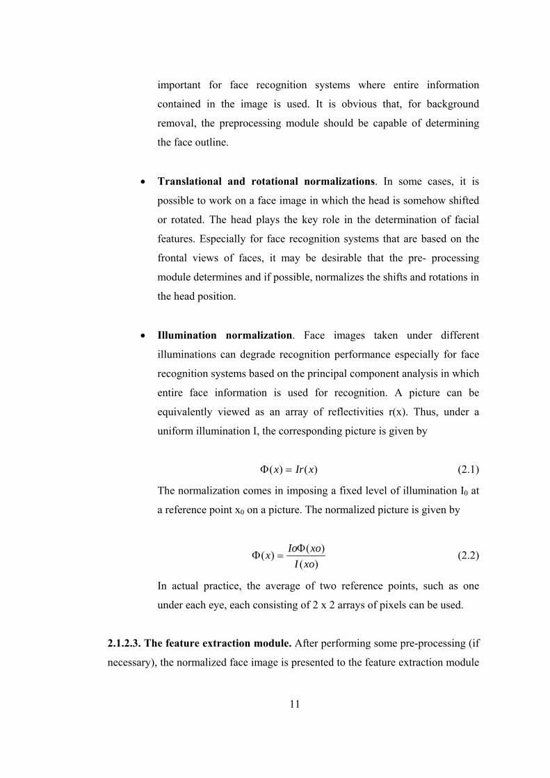
• Illumination normalization. Face images taken under different

illuminations can degrade recognition performance especially for face

recognition systems based on the principal component analysis in which

entire face information is used for recognition. A picture can be

equivalently viewed as an array of reflectivities r(x). Thus, under a

uniform illumination I, the corresponding picture is given by

)()( xIrx =Φ (2.1)

The normalization comes in imposing a fixed level of illumination I0 at

a reference point x0 on a picture. The normalized picture is given by

)(

)()(xoI

xoIox Φ=Φ (2.2)

In actual practice, the average of two reference points, such as one

under each eye, each consisting of 2 x 2 arrays of pixels can be used.

2.1.2.3. The feature extraction module. After performing some pre-processing (if

necessary), the normalized face image is presented to the feature extraction module

11

in order to find the key features that are going to be used for classification. In other

words, this module is responsible for composing a feature vector that is well

enough to represent the face image.

2.1.2.4. The classification module. In this module, with the help of a pattern

classifier, extracted features of the face image is compared with the ones stored in a

face library (or face database). After doing this comparison, face image is classified

as either known or unknown.

2.1.2.5. Training set. Training sets are used during the "learning phase" of the face

recognition process. The feature extraction and the classification modules adjust

their parameters in order to achieve optimum recognition performance by making

use of training sets.

2.1.2.6. Face library or face database. After being classified as "unknown", face

images can be added to a library (or to a database) with their feature vectors for

later comparisons. The classification module makes direct use of the face library.

2.1.3. Problems that May Occur During Face Recognition

Due to the dynamic nature of face images, a face recognition system encounters

various problems during the recognition process. It is possible to classify a face

recognition system as either "robust" or "weak" based on its recognition

performances under these circumstances. The objectives of a robust face

recognition system are given below:

2.1.3.1. Scale invariance. The same face can be presented to the system at

different scales as shown in Figure 2.2-b. This may happen due to the focal

distance between the face and the camera. As this distance gets closer, the face

image gets bigger.

12

2.1.3.2. Shift invariance. The same face can be presented to the system at different

perspectives and orientations as shown in Figure 2.2-c. For instance, face images of

the same person could be taken from frontal and profile views. Besides, head

orientation may change due to translations and rotations.

2.1.3.3. Illumination invariance. Face images of the same person can be taken

under different illumination conditions such as, the position and the strength of the

light source can be modified like the ones shown in Figure 2.2-d.

2.1.3.4 Emotional expression and detail invariance. Face images of the same

person can differ in expressions when smiling or laughing. Also, like the ones

shown in Figure 2.2-e, some details such as dark glasses, beards or moustaches can

be present.

2.1.3.5. Noise invariance. A robust face recognition system should be insensitive to

noise generated by frame grabbers or cameras. Also, it should function under

partially occluded images. A robust face recognition system should be capable of

classifying a face image as "known" under even above conditions, if it has already

been stored in the face database.

13

Figure 2.2 (a) Original face image

(b) Scale variance

(c) Orientation variance

(d) Illumination variance

(e) Presence of details

2.1.4. Feature Based Face Recognition

It was mentioned before that, there were two basic approaches to the face

recognition problem: Feature based face recognition and principal component

analysis methods. Although feature based face recognition can be divided into two

different categories, based on frontal views and profile silhouettes, they share some

common properties and we will treat them as a whole. In this section, basic

principals of feature based face recognition from frontal views [33] are presented.

2.1.4.1. Introduction

The first step of human face identification is to extract the features from facial

images. In the area of feature selection, the question has been addressed in studies

of cue salience in which discrete features such as the eyes, mouth, chin and nose

have been found important cues for discrimination and recognition of faces.

After knowing what the effective features are for face recognition, some

methods should be utilized to get contours of eyes, eyebrows, mouth, nose, and

14

face. For different facial contours, different models should be used to extract them

from the original portrait. Because the shapes of eyes and mouth are similar to some

geometric figures, they can be extracted in terms of the deformable template model

[27]. The other facial features such as eyebrows nose and face are so variable that

they have to be extracted by the active contour model [34, 35]. These two models

can be illustrated in the following:

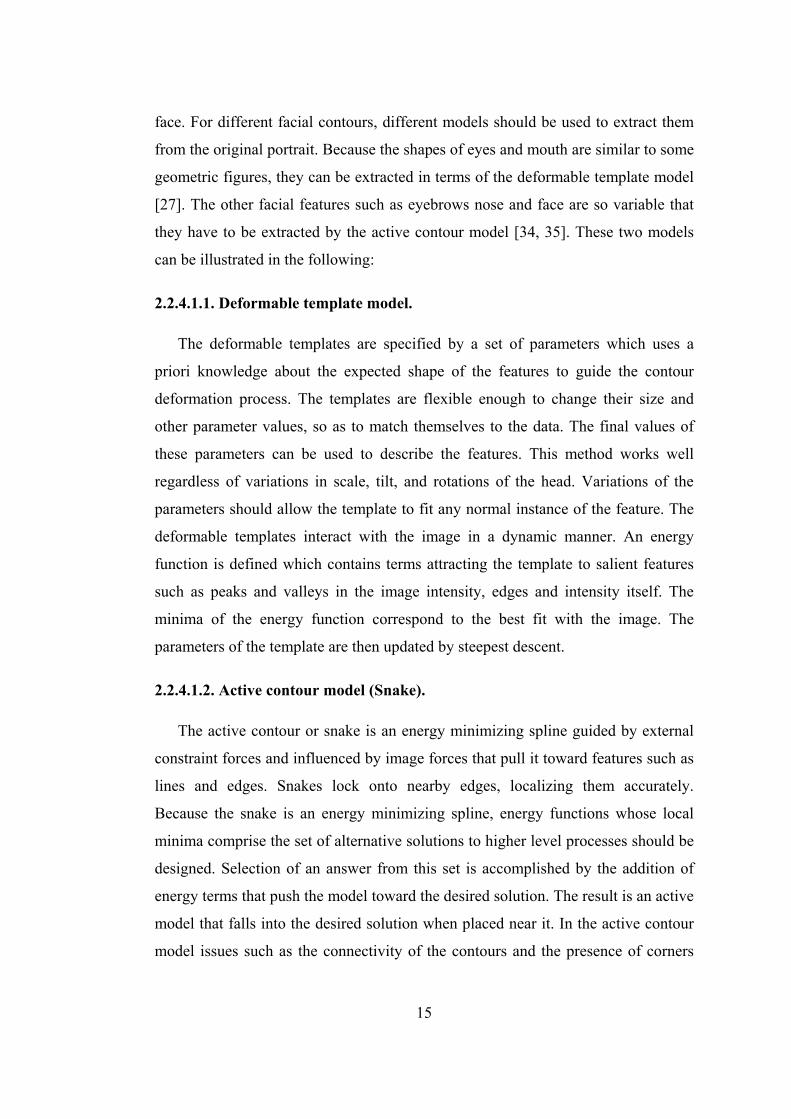
2.2.4.1.1. Deformable template model.

The deformable templates are specified by a set of parameters which uses a

priori knowledge about the expected shape of the features to guide the contour

deformation process. The templates are flexible enough to change their size and

other parameter values, so as to match themselves to the data. The final values of

these parameters can be used to describe the features. This method works well

regardless of variations in scale, tilt, and rotations of the head. Variations of the

parameters should allow the template to fit any normal instance of the feature. The

deformable templates interact with the image in a dynamic manner. An energy

function is defined which contains terms attracting the template to salient features

such as peaks and valleys in the image intensity, edges and intensity itself. The

minima of the energy function correspond to the best fit with the image. The

parameters of the template are then updated by steepest descent.

2.2.4.1.2. Active contour model (Snake).

The active contour or snake is an energy minimizing spline guided by external

constraint forces and influenced by image forces that pull it toward features such as

lines and edges. Snakes lock onto nearby edges, localizing them accurately.

Because the snake is an energy minimizing spline, energy functions whose local

minima comprise the set of alternative solutions to higher level processes should be

designed. Selection of an answer from this set is accomplished by the addition of

energy terms that push the model toward the desired solution. The result is an active

model that falls into the desired solution when placed near it. In the active contour

model issues such as the connectivity of the contours and the presence of corners

15

affect the energy function and hence the detailed structure of the locally optimal

contour. These issues can be resolved by very high-level computations.

2.1.4.2. Effective Feature Selection

Before mentioning the facial feature extraction procedures, we have the

following two considerations:

1. The picture-taking environment must be fixed in order to get a good snapshot.

2. Effective features that can be used to identify a face efficiently should be

known.

Despite the marked similarity of faces as spatial patterns we are able to

differentiate and remember a potentially unlimited number of faces. With sufficient

familiarity, the faces of any two persons can be discriminated. The skill depends on

the ability to extract invariant structural information from the transient situation of a

face, such as changing hairstyles, emotional expression, and facial motion effect.

Features are the basic elements for object recognition. Therefore, to identify a

face, we need to know what features are used effectively in the face recognition

process. Because the variance of each feature associated with the face recognition

process is relatively large, the features are classified into three major types:

2.1.4.2.1. First-order features values.

Discrete features such as eyes, eyebrows, mouth, chin, and nose, which have

been found to be important [4] in face identification and are specified without

reference to other facial features, are called first-order features. Important first-order

features are given in Table 2.1.

2.1.4.2.2. Second-order features values.

Another configurable set of features which characterize the spatial relationships

between the positions of the first-order features and information about the shape of

16

the face are called second-order features. Important second-order features are given

in Table 2.2. Second order features that are related to nose, if nose is noticeable are

given in Table 2.3.

2.1.4.2.3 Higher-order feature values.

There are also higher-level features whose values depend on a complex set of

feature values. For instance, age might be a function of hair coverage, hair color,

skin tension, presence of wrinkles and age spots, forehead height which changes

because of receding hairline, and so on.

Variability such as emotional expression or skin tension exists in the higher-

order features and the complexity, which is the function of first-order and second-

order features, is very difficult to predict. Permanent information belonging to the

higher-order features can not be found simply by using first and second-order

features. For a robust face recognition system, features that are invariant to the

changes of the picture taking environment should be used. Thus, these features may

contain merely first-order and second-order ones. These effective feature values

cover almost all the obtainable information from the portrait. They are sufficient for

the face recognition process.

The feature values of the second-order are more important than those of the

first-order and they are dominant in the feature vector. Before mentioning the facial

feature extraction process, it is necessary to deal with two preprocessing steps:

Threshold assignment. Brightness threshold should be known in order to

discriminate the feature and other areas of the face. Generally, different

thresholds are used for eyebrows, eyes, mouth, nose, and face according to

the brightness of the picture.

Rough Contour Estimation Routine (RCER). The left eyebrow is the first

feature that is to be extracted. The first step is to estimate the rough contour

of the left eyebrow and find the contour points. Generally, the position of

the left eyebrow is about one-fourth of the facial width. Having this a priori

17

information, the coarse position of the left eyebrow can be found and its

rough contour can be captured. Once the rough contour of the left eyebrow

is established, the rough contours of other facial features such as left eye,

right eyebrow, mouth or nose can be estimated by RCER [29]. After the

rough contour is obtained, its precise contour will be extracted by the

deformable template model or the active contour model.

Table 2.1 First-order features

Measurement Facial Location left eyebrow right eyebrow left eye right eye mouth

Area, angle

face Length of left eyebrow Length of right eyebrow Length of left eye Length of right eye Length of mouth Length of face

Distance

Height of face

18

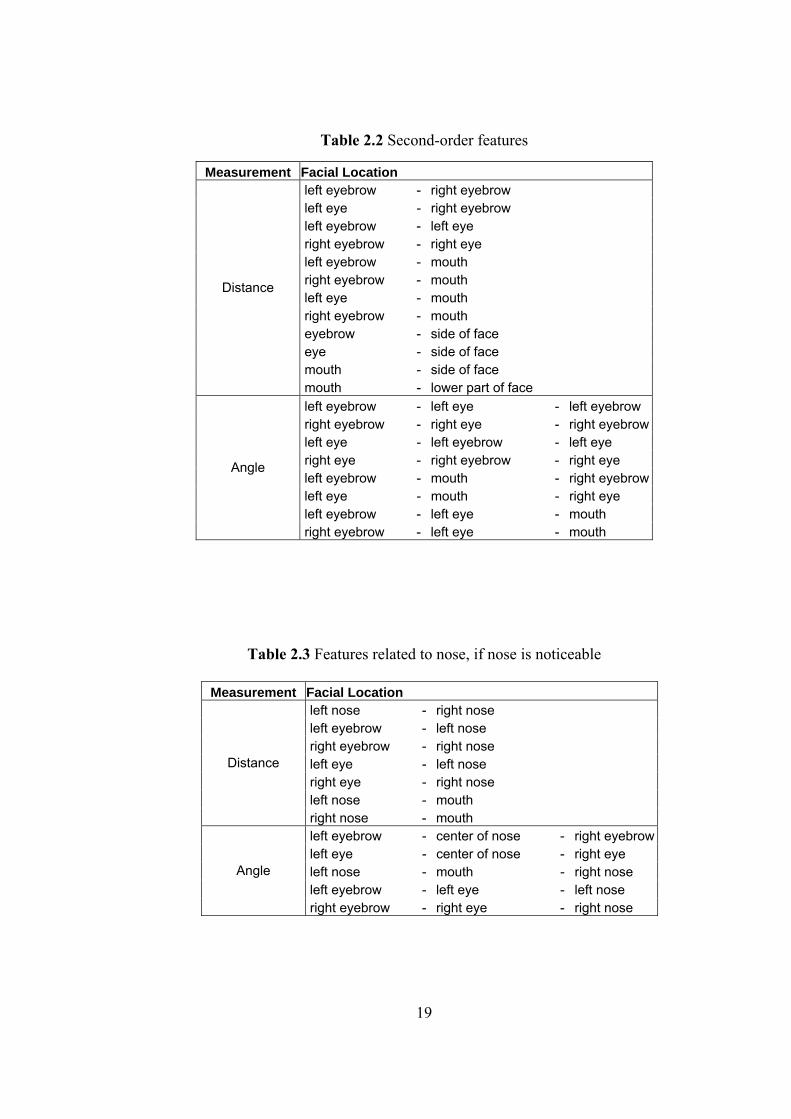
Table 2.2 Second-order features

Measurement Facial Location

left eyebrow - right eyebrow left eye - right eyebrow left eyebrow - left eye right eyebrow - right eye left eyebrow - mouth right eyebrow - mouth left eye - mouth right eyebrow - mouth eyebrow - side of face eye - side of face mouth - side of face

Distance

mouth - lower part of face left eyebrow - left eye - left eyebrow right eyebrow - right eye - right eyebrow left eye - left eyebrow - left eye right eye - right eyebrow - right eye left eyebrow - mouth - right eyebrow left eye - mouth - right eye left eyebrow - left eye - mouth

Angle

right eyebrow - left eye - mouth

Table 2.3 Features related to nose, if nose is noticeable

Measurement Facial Location left nose - right nose left eyebrow - left nose right eyebrow - right nose left eye - left nose right eye - right nose left nose - mouth

Distance

right nose - mouth left eyebrow - center of nose - right eyebrow left eye - center of nose - right eye left nose - mouth - right nose left eyebrow - left eye - left nose

Angle

right eyebrow - right eye - right nose

19

2.1.4.3. Feature Extraction Using the Deformable Templates

After the rough contour is obtained, the next step of face recognition is to find

the physical contour of each feature. Conventional edge detectors can not find facial

features such as the contours of the eye or mouth accurately from local evidence of

edges, because they can not organize local information into a sensible global

perception. There is a method to detect the contour of the eye by the deformable

template which was originally proposed by Yullie [27]. It is possible to reduce

computations at the cost of the precision of the extracted contour.

2.1.4.3.1. Eye Template

The deformable template acts on three representations of the image, as well as

on the image itself. The first two representations are the peak and valleys in the

image intensity and the third is the place where the image intensity changes quickly.

The eye template developed by Yullie et al. consists of the following features:

• A circle of radius r, centered on a point (xc , yc) , corresponding to the

iris. The boundaries of the iris and the whites of the eyes are attracted to

edges the image intensity. The interior of the circle is attracted to

valleys, or low values in the image intensity.

• A bounding contour of the eye attracted to edges. This contour is

modeled by two parabolic sections representing the upper and lower

parts of the boundary. It has a center (xc , yc), with 2w, maximum height

h1 of the boundary above the center, maximum height h2 of the boundary

below the center, and an angle of rotation.

• Two points, corresponding to the centers for the whites of the eyes,

which are attracted to peaks in the image intensity.

20

• Regions between the bounding contour and the iris which also

correspond to the whites of the eyes. These will be attracted to large

intensity values.

The original eye template can be modified for the sake of simplicity where the

accuracy of the extracted contour is not critical. The lack of a circle does not affect

the classified results because the feature values are obtained from other information.

The upper and lower parabola will be satisfactory for the recognition process. Thus,

the total energy function for the eye template can be defined a combination of the

energy functions of edge, white and black points.

The total energy function is defined as

E total = E edge + E white + E black (2.3)

where E edge , E white , E black are defined in the following:

• The edge potentials are given by the integral over the curves of the upper

and lower parabola divided by their length:

dsyx

lengthlowerw

dsyxlengthupper

wE

boundloweredge

boundupperedgeedge

),(_

),(_

_

2

_

1

∫

∫

Φ−

Φ−=

(2.4)

where upper-bound and lower-bound represent the upper and lower parts of the eye,

and Фedge represents the edge response of the point (x,y).

• The potentials of white and black points are defined as the integral over

the area bounded by the upper and lower parabola divided by the area:

dAyxNwyxNwArea

E whıhıwareapara

blackbbw )),(),((1, +−−= ∫∫

−

(2.5)

21

where N black (x , y ) and N white(x , y) represent the number of black and white points,

and wb , ww are weights related with black and white points.

In order to be not affected by an improper threshold, the black and white

points in Eq.(2.5) are defines as

P(x,y) is a black point if I(x,y) ≤ (threshold - tolerance),

P(x,y) is a white point if I(x,y) ≥ (threshold + tolerance),

P(x,y) is an unambiguous point if I(x,y) is in between. (2.6)

where I(x,y) is the image intensity at point (x,y).

By the energy functions defined above, we can calculate the energy in the

range of little modulations of 2w, h1 , h2 and ф. When the minimum energy value

takes place, the precise contour is extracted.

2.1.4.3.2. Mouth Template

In the whole features of the front view of the face, the role of the mouth in

relatively important. The properties of the mouth contour are heavily involved in

the face recognition process. The deformable mouth template changes its own shape

when it comes across the image areas of edge (which the intensity changes quickly),

and white and black points. Generally, features related to middle lips, lower and

upper lips are extracted. Because of the effect of brightness in the picture taking

period, the middle of the lower lip may not be apparent. RCER can not find the

approximate height of the lower lip. Fortunately, the length of the mouth can still be

found by RCER. Usually, the height of the lower lip is between one-fourth and one-

sixth of the mouth's length.

The mouth contour energy function consists of the edge term E edge and the black

term E black . The edge term dominates at the edge area, where as the black term

encloses as many black points belonging to the mouth as possible.

Etotal = Eedge + E black (2.7)

22

• The edge energy function consists of three parts: middle lip (gap

between lips), lower lip and upper lip separated at philtrum. The

equation of the middle lip part is

dsyxrightw

dsyxleftw

dsyxlowerw

Eright

edgeright

leftedge

left

loweredge

loweredge ),(),(),( ∫∫∫ Φ−Φ−Φ−=

(2.8)

where lower represents the lower boundary of mouth, left represents the left part of

upper lip, right represents the right part of upper lip, and Фedge (x,y) represent the

edge response of point (x,y).

• The black energy function helps the edge energy to enclose black points

belonging to the mouth and is defined as:

dSyxNwlengthmid

dAyxNwArea

Emıı

blackmidblackblack

ubound

lboundblack ),(

_1),(1

∫∫∫ −+−=

(2.9)

where Lbound represents lower lip, Ubound represents upper lip, and mid represents

number of black points. The black points are defined by Eq. (2.6) The weights

wblack , wmid , wlower , wleft and wright are experimentally determined.

2.1.4.4. Feature Extraction Using the Active Contour

The shapes of eyebrow, nostril and face, unlike eye and mouth, are even

more different for different people and their contours can not be captured by using

the deformable template. In this case, the active contour model or the "snake" is

used. A snake is an energy minimizing spline guided by external constraint forces

and influenced by image forces that pull it toward features such as lines and edges.

This approach differs from traditional approaches which detect edges and then links

them. In the active contour model, image and external forces together with the

connectivity of the contours and the presence of corners will affect the energy

23

function and the detailed structure of the locally optimal contour. The energy

function of the active contour model [35] is defined

as:

dSsvEdSsvEdSsvEdSsvEE sconstraıonimagesernalsnakesnake ))(())(())(())((1

0

1

0

1

0 int

1

0 ∫∫∫∫ ++==

(2.10)

where v(s) represents the position of the snake, E ernal int represents the internal

energy of the contour due to bending, E images gives rise to the image forces, and

Econs traint represents the external energy.

2.1.4.4.1. The Modified Active Contour Model

The original active contour model is user interactive. The advantage of its being

user interactive is that the final form of the snake can be influenced by feedback

from a higher level process. As the algorithm iterates the energy terms can be

adjusted by higher level processes to obtain a local minima that seems most useful

to that process. However, there are some problems with minimization procedure.

Amini et al [37], pointed out some problems including instability and a tendency for

points to bunch up on a strong portion of an edge. They proposed a dynamic

programming algorithm for minimizing the energy function. Their approach had the

advantage of using points on the discrete grid and is numerically stable, however

the convergence is very slow.

It is possible to find a faster algorithm for the active contour [36]. Although

this model still has the disadvantage of being unable to guarantee global minima, it

can solve the problem of bunching up on a strong portion in the active contour. This

problem occurs during the iterative process when contour points will accumulate at

certain strong portions of the active contour. Besides, its computation speed is faster

and thus, it is more suitable for face recognition. Active contour energy can be

redefined [33] as:

24

dSsvimagescurvaturecontinuitytotal ExsvEssvEsE ))((

1

0

)(())(()(())(())(( δβα ++= ∫ (2.11)

The definition of v(s) is similar to Eq (2.13) and the following

approximations are used:

2112

22

1 2 +−− +−≈−≈ iiii

iii vvv

dsvd

andvvdsdv

(2.12)

• Continuity force. The first derivative vi – vi-12 causes the curve to

shrink. It is actually minimizing the distance between points. It also

contributes to the problem of points bunching up on strong portions of

the contour. It was decided that a term which encouraged even spacing

of the points would satisfy the original goal of first order continuity

without the effect of shrinking.

Here, this term uses the difference between the average distance points,

d, and this distance between the two points under consideration,

d -vi – vi-1 Thus points having a distance near the average will

have the minimum value. At the end of each iteration a new value of d is

computed.

• Curvature force. Since the formulation of the continuity term causes

the points to be relatively evenly spaced, vi-1 – 2vi + vi+12 gives a

reasonable

and quick estimate of the curvature. This term, like the continuity term,

is normalized by dividing the largest value in the neighborhood, giving a

number from 0 to 1.

25

• Image force. E images is the image force which is defined by the

following operations:

1. We have eight image energy measurements (Mag), for eight

neighbors.

2. To normalize the image energy measurements, we select the

minimum (Min), and maximum (Max) terms from those eight

measurements, and then do the calculation, (Min - Max)/(Max - Min)

to obtain the image force.

At the end of each iteration, the curvature is determined at each point on the new

contour. If the value is larger than the threshold, β is set to 0 for the next iteration.

The greedy algorithm [36] is applied for fast convergence. The energy function is

computed for the current location of vi and each of its neighbors. The neighbor

having the smallest value is chosen as the new position of vi . The greedy algorithm

can be applied to extract the features of eyebrow, nostril, and face. In order to

prevent the snake failing at inaccurate local minima, contour estimation is done via

RCER before the snake iterates. RCER uses a priori knowledge to find a rough

contour as a starting (initial) contour for the snake.

2.1.4.4.2. Boundary Extraction of a Face

In order to demonstrate the use of active contour models on facial contour

extraction, energy function associated to the boundary extraction of a face is

presented in this section.

Unlike eyebrow extraction, the boundary extraction of a face is more time

consuming because the rough contour of a face can not be estimated by RCER.

However, the rough contour needs to be approximated as accurately as possible.

The energy function associated with boundary extraction of a face is defined as

)(1

imagesicurvatureicontinuity

n

iiface EEEE δβα ++= ∑

=

(2.13)

26

where E continuity and E curvature are defined in section 2.1.4.4.1 and E images is defined

as

Eimages = w lines E lines + w edge E edge (2.14)

The goal of E lines is to attract more white points and less dark ones inside the active

contour, where as the goal of E edge is to attract more edge points on the active

contour boundary.

E lines and E edge are defined as

(2.15),

(2.16)

where I(x,y) represents the intensity value of point (x,y), threshold is the same as

face threshold, tolerance is experimentally determined.

To extract the boundary of a face without a beard, the snake iterates and moves

toward the chin because E face decreases constantly. The convergent process of the

snake is based on the greedy algorithm. When the iterative process stops, iterations

can be re-started in order to find its next convergent place. If they are similar, the

position is accurate.

27

2.1.5. Face Recognition Based on Principal Component Analysis

In section 2.1.4, we have reviewed a face recognition method based on feature

extraction. By using extensive geometry, it is possible to find the contours of the

eye, eyebrow, nose, mouth, and even the face itself.

Principal component analysis for face recognition is based on the

information theory approach. Here, the relevant information in a face image is

extracted and encoded as efficiently as possible. Recognition is performed on a face

database that consists of models encoded similarly.

In mathematical terms, the principal components of the distribution of faces

or the eigenvectors of the covariance matrix of the set of face images, treating an

image as a point (vector) in a very high dimensional face space is sought. In

Chapter 3, a principal component analysis method will be presented in more detail.

28

CHAPTER 3

FACE RECOGNITION USING EIGENFACES

The aim of this chapter is to introduce the explanation of a principal

component analysis and usage of neural networks for face recognition. For principal

component analysis, eigenface method will be used for extracting feature vectors.

3.1. Introduction

Much of the previous work on automated face recognition has ignored the

issue of just what aspects of the face stimulus are important for face recognition.

This suggests the use of an information theory approach of coding and decoding of

face images, emphasizing the significant local and global features. Such features

may or may not be directly related to our intuitive notion of face features such as

the eyes, nose, lips, and hair.

In the language of information theory, the relevant information in a face

image is extracted, encoded as efficiently as possible, and then compared with a

database of models encoded similarly. A simple approach to extracting the

information contained in an image of a face is to somehow capture the variation in a

collection of face images, independent of any judgment of features, and use this

information to encode and compare individual face images.

In mathematical terms, the principal components of the distribution of faces,

or the eigenvectors of the covariance matrix of the set of face images, treating an

image as point (or vector) in a very high dimensional space is sought. The

29

eigenvectors are ordered, each one accounting for a different amount of the

variation among the face images.

These eigenvectors can be thought of as a set of features that together

characterize the variation between face images. Each image location contributes

more or less to each eigenvector, so that it is possible to display these eigenvectors

as a sort of ghostly face image which is called an "eigenface".

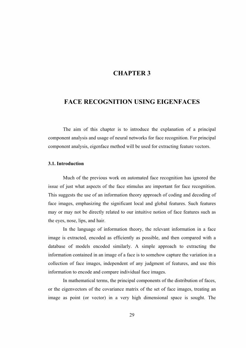
Sample face images, the average face of them, eigenfaces of the face images

and the corresponding eigenvalues are shown in Figure 3.1, Figure 3.2, Figure 3.3,

and Figure 3.4 respectively. Each eigenface deviates from uniform gray where some

facial feature differs among the set of training faces. Eigenfaces can be viewed as a

sort of map of the variations between faces.

Figure 3.1 Sample Faces

30

Figure 3.2 Average face of the Sample Faces

Figure 3.3 Eigen Faces of the Sample Faces

31

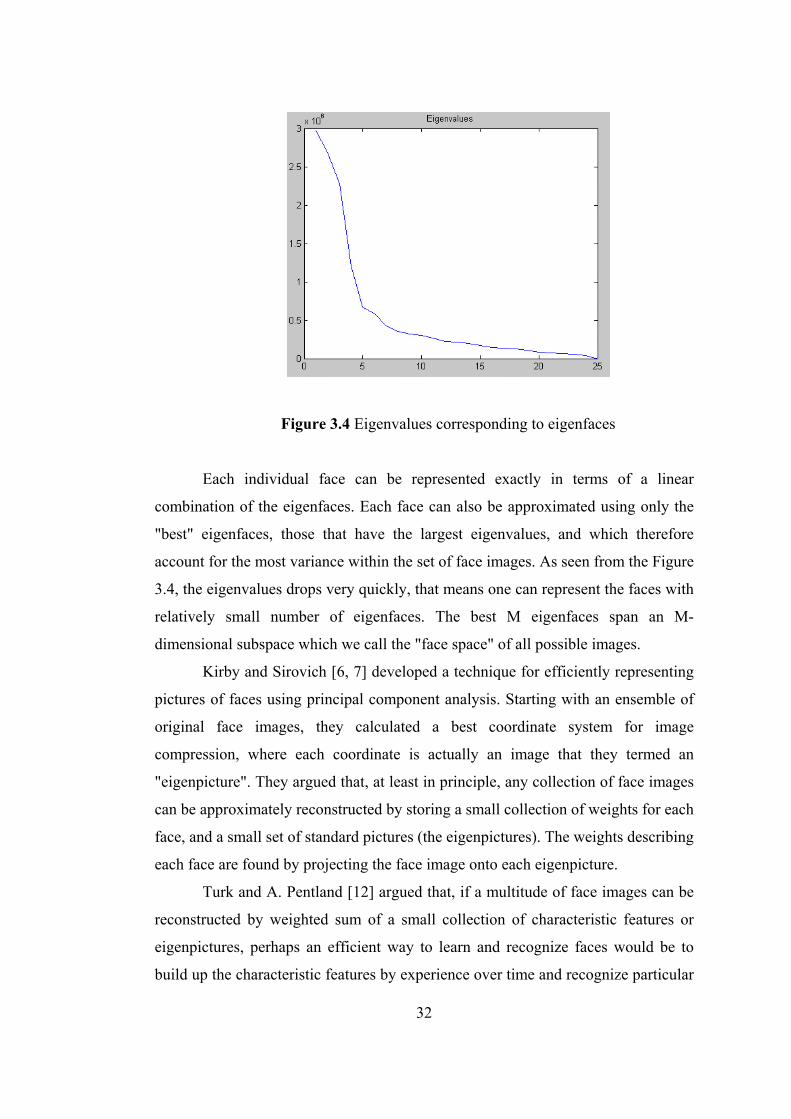
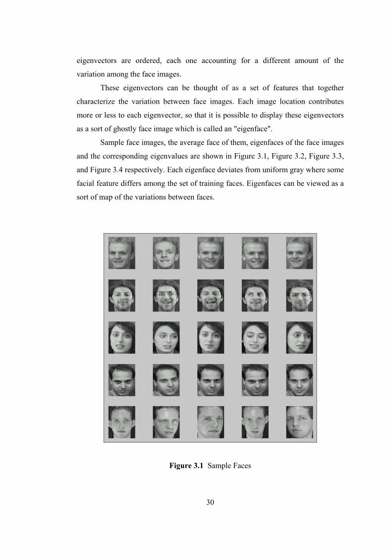
Figure 3.4 Eigenvalues corresponding to eigenfaces

Each individual face can be represented exactly in terms of a linear

combination of the eigenfaces. Each face can also be approximated using only the

"best" eigenfaces, those that have the largest eigenvalues, and which therefore

account for the most variance within the set of face images. As seen from the Figure

3.4, the eigenvalues drops very quickly, that means one can represent the faces with

relatively small number of eigenfaces. The best M eigenfaces span an M-

dimensional subspace which we call the "face space" of all possible images.

Kirby and Sirovich [6, 7] developed a technique for efficiently representing

pictures of faces using principal component analysis. Starting with an ensemble of

original face images, they calculated a best coordinate system for image

compression, where each coordinate is actually an image that they termed an

"eigenpicture". They argued that, at least in principle, any collection of face images

can be approximately reconstructed by storing a small collection of weights for each

face, and a small set of standard pictures (the eigenpictures). The weights describing

each face are found by projecting the face image onto each eigenpicture.

Turk and A. Pentland [12] argued that, if a multitude of face images can be

reconstructed by weighted sum of a small collection of characteristic features or

eigenpictures, perhaps an efficient way to learn and recognize faces would be to

build up the characteristic features by experience over time and recognize particular

32

faces by comparing the feature weights needed to approximately reconstruct them

with the weights associated with known individuals. Therefore, each individual is

characterized by a small set of feature or eigenpicture weights needed to describe

and reconstruct them. This is an extremely compact representation when compared

with the images themselves. The projected image of the Face1 with a number of

eigenvalues is shown in Figure3.5. As seen from the figure among the 25 faces

database (25 eigenfaces), 15 eigenfaces are enough for reconstruct the faces

accurately. These feature or eigenpicture weights are called feature vectors and as

seen in Section 3.3, they will be used as new descriptors of the face images and

used fro recognition purposes.

Figure 3.5 Reconstruction of First Image with the number of Eigenfaces.

33

3.2. Calculation of Eigenfaces

Let a face image I(x,y) be a two-dimensional N x N array of 8-bit intensity

values. An image may also be considered as a vector of dimension N2, so that a

typical image of size 256 x 256 becomes a vector of dimension 65,536, or

equivalently a point in 65,536-dimensional space. An ensemble of images, then,

maps to a collection of points in this huge space.

Images of faces, being similar in overall configuration, will not be randomly

distributed in this huge image space and thus can be described by a relatively low

dimensional subspace. The main idea of the principal component analysis (or

Karhunen-Loeve expansion) is to find the vectors that best account for the

distribution of face images within the entire image space.

These vectors define the subspace of face images, which we call "face

space". Each vector is of length N,2 describes an N x N image, and is a linear

combination of the original face images. Because these vectors are the eigenvectors

of the covariance matrix corresponding to the original face images, and they are

face-like in appearance, we refer to them as "eigenfaces". Some examples of

eigenfaces are shown in Figure 3.3.

Definitions:

An N x N matrix A is said to have an eigenvector X, and corresponding

eigenvalue λ if

AX = λX. (3.1)

Evidently, Eq. (3.1) can hold only if

detA -λ I = 0 (3.2)

which, if expanded out, is an Nth degree polynomial in λ whose root are the

eigenvalues. This proves that there are always N (not necessarily distinct)

eigenvalues. Equal eigenvalues coming from multiple roots are called "degenerate".

34

A matrix is called symmetric if it is equal to its transpose,

A= AT or aij = aji (3.3)

it is termed orthogonal if its transpose equals its inverse,

AT A = AAT =I (3.4)

finally, a real matrix is called normal if it commutes with is transpose,

AT A = AAT (3.5)

Theorem: Eigenvalues of a real symmetric matrix are all real. Contrariwise, the

eigenvalues of a real nonsymmetric matrix may include real values, but may also

include pairs of complex conjugate values. The eigenvalues of a normal matrix with

nondegenerate eigenvalues are complete and orthogonal, spanning the N

dimensional vector space.

After giving some insight on the terms that are going to be used in the

evaluation of the eigenfaces, we can deal with the actual process of finding these

eigenfaces.

Let the training set of face images be Г1 Г2…………. ГM, then the average of

the set is defined by

∑=

Γ=ΨM

nnM 1

1 (3.6)

Each face differs from the average by the vector

Ф i = Г i –Ψ (3.7)

An example training set is shown in Figure 3.1, with the average face Ψ

shown in Figure 3.2.

35

This set of very large vectors is then subject to principal component

analysis, which seeks a set of M orthonormal vectors, un , which best describes the

distribution of the data. The kth vector, uk , is chosen such that

2

1)(1 ∑

=

Φ=M

nn

Tkk u

Mλ (3.8)

is a maximum, subject to

1, if l=k

ul uk = δlk = (3.9)

0, otherwise

The vectors uk and scalars lk are the eigenvectors and eigenvalues,

respectively of the covariance matrix

)(11

Tn

M

nnM

C ΦΦ= ∑=

= A AT (3.10)

where the matrix A= [Ф1 Ф2 …… ФM ]. The covariance matrix C, however

is N2 x N2 real symmetric matrix, and determining the N2 eigenvectors and

eigenvalues is an intractable task for typical image sizes. We need a

computationally feasible method to find these eigenvectors.

If the number of data points in the image space is less than the dimension of

the space (M < N2), there will be only M-1, rather than N2, meaningful

eigenvectors. The remaining eigenvectors will have associated eigenvalues of zero.

We can solve for the N2 dimensional eigenvectors in this case by first solving the

eigenvectors of an M x M matrix such as solving 16 x 16 matrix rather than a

16,384 x 16,384 matrix and then, taking appropriate linear combinations of the face

images Фi .

Consider the eigenvectors vi of A AT such that

AT Avi = µi vi (3.11)

36

Premultiplying both sides by A, we have

AAT Avi = µi Avi (3.12)

from which we see that Avi are the eigenvectors of C= AAT

Following these analysis, we construct the M x M matrix L = AAT, where

Lmn = ФmT Фn and find the M eigenvectors, vl , of L. These vectors determine linear

combinations of the M training set face images to form the eigenfaces ul .

(3.13) k

M

klkl vu Φ= ∑

=1

With this analysis, the calculations are greatly reduced, from the order of the

number of pixels in the images (N2) to the order of the number of images in the

training set (M). In practice, the training set of face images will be relatively small

(M << N2 ), and the calculations become quite manageable. The associated

eigenvalues allow us to rank the eigenvectors according to their usefulness in

characterizing the variation among the images.

The success of this algorithm is based on the evaluation of the eigenvalues

and eigenvectors of the real symmetric matrix L that is composed from the training

set of images. Root searching in the characteristic equation, Eq. (3.2) is usually a

very poor computational method for finding eigenvalues. During the programming

phase of the above algorithm, a more efficient method [38] was used in order to

evaluate the eigenvalues and eigenvectors. At first, the real symmetric matrix is

reduced to tridiagonal form with the help of the "Householder" algorithm. The

Householder algorithm reduces an N x N symmetric matrix A to tridiagonal form

by N - 2 orthogonal transformations. Each transformation annihilates the required

part of a whole column and whole corresponding row. After that, eigenvalues and

eigenvectors are obtained with the help of QR transformations. The basic idea

behind the QR algorithm is that any real symmetric matrix can be decomposed in

37

the form A = QR where Q is orthogonal and R is upper triangular. The workload in

the QR algorithm is O(N3 ) per iteration for a general matrix, which is prohibitive.

However, the workload is only O(N) per iteration for a tridiagonal matrix, which

makes it extremely efficient.

3.3. Using Eigenfaces to Classify a Face Image

The eigenface images calculated from the eigenvectors of L, span a basis set

with which to describe face images. Sirovich and Kirby evaluated a limited version

of this framework on an ensemble of M = 115 images of Caucasian males digitized

in a controlled manner, and found that 40 eigenfaces were sufficient for a very good

description of face images. With M' = 40 eigenfaces, RMS pixel by pixel errors in

representing cropped versions of face images were about 2%.

In practice, a smaller M' can be sufficient for identification, since accurate

reconstruction of the image is not a requirement and, it was observed that, for a

training set of fourteen face images, seven eigenfaces were enough for a sufficient

description of the training set members. But for maximum accuracy, the number of

eigenfaces should be equal to the number of images in the training set.

In this framework, identification becomes a pattern recognition task. The

eigenfaces span an M' dimensional subspace of the original N2 image space. The M'

significant eigenvectors of the L matrix are chosen as those with the largest

associated eigenvalues.

A new face image (Г ) is transformed into its eigenface components

(projected onto "face space") by a simple operation,

w k =ukT (Г –Ψ ) (3.14)

for k = 1,...,M'. This describes a set of point by point image multiplications and

summations, operations performed at approximately frame rate on current image

processing hardware, with a computational complexity of O(N4 ).

38

The weights form a feature vector,

ΩT =[w1 w2…… wM ] (3.15)

that describes the contribution of each eigenface in representing the input face

image, treating the eigenfaces as a basis set for face images. The feature vector is

then used in a standard pattern recognition algorithm to find which of a number of

predefined face classes, if any, best describes the face. The face classes Ωi can be

calculated by averaging the results of the eigenface representation over a small

number of face images (as few as one) of each individual.

3.4. Rebuilding a Face Image with Eigenfaces

A face image can be approximately reconstructed (rebuilt) by using its feature

vector and the eigenfaces as

Г ‘ =Ψ + Ф f (3.16)

where

j

M

jjj uw∑

=

=Φ1

(3.17)

is the projected image.

Eq. (3.16) tells that the face image under consideration is rebuilt just by

adding each eigenface with a contribution of wi Eq. (3.17) to the average of the

training set images. The degree of the fit or the "rebuild error ratio" can be

expressed by means of the Euclidean distance between the original and the

reconstructed face image as given in Eq. (3.18).

Rebuild error ratio = Γ

Γ−Γ l

(3.18)

39

It has been observed that, rebuild error ratio increases as the training set

members differ heavily from each other. This is due to the addition of the average

face image. When the members differ from each other (especially in image

background) the average face image becomes messier and this increases the rebuild

error ratio.

3.5. Usage of Neural Networks for Recognition:

3.5.1. Introduction

Neural networks are composed of simple elements operating in parallel. The

neuron model shown in Figure 3.6 is the one that widely used in artificial neural

networks with some minor modifications on it.

W1

W2

Wj

WN

u1

u2

uj

N

a = ( ∑ wj uj ) + Ф x=f(a) j=1

x

uN

Figure 3.6 Artificial Neuron

The artificial neuron given in this figure has N input, denoted as u1, u2,…uN.

Each line connecting these inputs to the neuron is assigned a weight, which is

denoted as w1,w2,….,wN respectively. The threshold in artificial neuron is usually

represented by Ф and the activation is given by the formula:

40

(3.19) Φ+= ∑=

)(1

j

n

jjuwa

The inputs and weight are real values. A negative value for a weight indicates an

inhibitory connection while a positive value indicating excitatory one. If Ф is

positive, it is usually referred as bias. For its mathematical convenience (+) sign is

used in the activation formula. Sometimes, the threshold is combined for simplicity

into the summation part by assuming an imaginary input u0 = +1 and a connection

weight w0 = Ф. Hence the activation formula becomes

)(1

j

n

jjuwa ∑

=

= (3.20)

The vector notation

A = wT u + Ф (3.21)

is useful for expressing the activation for a neuron.

The neuron output function f(a) can be:

Linear :

aKaf ()( = ) (3.22)

Threshold :

(3.23) ⎩⎨⎧

<≤

=a

aaf

0100

)(

Ramp:

(3.24) ⎪⎩

⎪⎨

⎧

<<≤

=aKaKa

aaf

10/

00)(

Sigmoid :

))exp(1/(1)( Kaaf −+= (3.25)

41

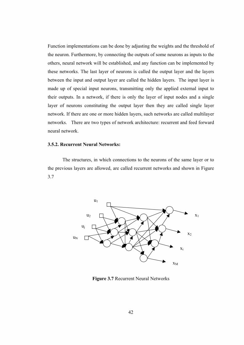
Function implementations can be done by adjusting the weights and the threshold of

the neuron. Furthermore, by connecting the outputs of some neurons as inputs to the

others, neural network will be established, and any function can be implemented by

these networks. The last layer of neurons is called the output layer and the layers

between the input and output layer are called the hidden layers. The input layer is

made up of special input neurons, transmitting only the applied external input to

their outputs. In a network, if there is only the layer of input nodes and a single

layer of neurons constituting the output layer then they are called single layer

network. If there are one or more hidden layers, such networks are called multilayer

networks. There are two types of network architecture: recurrent and feed forward

neural network.

3.5.2. Recurrent Neural Networks:

The structures, in which connections to the neurons of the same layer or to

the previous layers are allowed, are called recurrent networks and shown in Figure

3.7

xM

xi

x2

x1

uN

uj

u2

u1

Figure 3.7 Recurrent Neural Networks

42

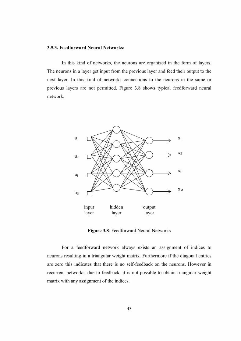
3.5.3. Feedforward Neural Networks:

In this kind of networks, the neurons are organized in the form of layers.

The neurons in a layer get input from the previous layer and feed their output to the

next layer. In this kind of networks connections to the neurons in the same or

previous layers are not permitted. Figure 3.8 shows typical feedforward neural

network.

u1

u2

uj

uN

outputlayer

hiddenlayer

input layer

xM

xi

x2

x1

Figure 3.8. Feedforward Neural Networks

For a feedforward network always exists an assignment of indices to

neurons resulting in a triangular weight matrix. Furthermore if the diagonal entries

are zero this indicates that there is no self-feedback on the neurons. However in

recurrent networks, due to feedback, it is not possible to obtain triangular weight

matrix with any assignment of the indices.

43

3.5.4. Training and Simulation of Neural Networks for Recognition

Neural networks have been trained to perform complex functions in various

fields of application including pattern recognition, identification, classification,

speech, vision and control systems.

In this thesis, there is one neural network for each person in the database.

After calculating eigenfaces, the feature vectors are calculated for the faces in the

database. These feature vectors are used as inputs to train the each person’s

networks. In training algorithm, the faces feature vectors that belong to same person

are used as positive examples for the person’s network (such that network gives ”1”

as output), and negative examples for the others network. (such that network gives

”0” as output), Figure 3.9 shows schematic diagram for the networks training.

When the new image is come for recognition, its feature vectors are

calculated from the eigenfaces found before, and this image gets its new descriptors.

These new descriptors are inputted to every network and the networks are simulated

with these descriptors.. The network outputs are compared. If the maximum output

exceeds the predefined threshold level, then this new face is decided to belong to

person with this maximum output.

44

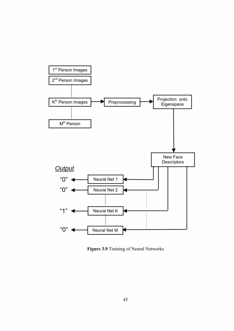
Projection onto Eigenspace

New Face Descriptors

Neural Net 1

Neural Net 2

Neural Net K

Preprocessing

2nd Person Images

Kth Person Images

Mth Person

Neural Net M

“0” “0”

“1”

“0”

Output

1st Person Images

Figure 3.9 Training of Neural Networks

45

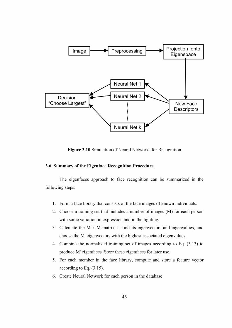
Image Projection onto Eigenspace

New Face Descriptors

Neural Net 1

Neural Net 2

Neural Net k

Preprocessing

Decision “Choose Largest”

Figure 3.10 Simulation of Neural Networks for Recognition

3.6. Summary of the Eigenface Recognition Procedure

The eigenfaces approach to face recognition can be summarized in the

following steps:

1. Form a face library that consists of the face images of known individuals.

2. Choose a training set that includes a number of images (M) for each person

with some variation in expression and in the lighting.

3. Calculate the M x M matrix L, find its eigenvectors and eigenvalues, and

choose the M' eigenvectors with the highest associated eigenvalues.

4. Combine the normalized training set of images according to Eq. (3.13) to

produce M' eigenfaces. Store these eigenfaces for later use.

5. For each member in the face library, compute and store a feature vector

according to Eq. (3.15).

6. Create Neural Network for each person in the database

46

7. Train these networks as the faces will be used as positive examples for their

own networks and negative examples for all other networks

8. For each new face image to be identified, calculate its feature vector

according to Eq. (3.15).

9. Use these feature vectors as network inputs and simulate all networks with

these inputs

10. Select the network with the maximum output. If the output of the selected

network passes a predefined threshold, it will be reported as the host of the

input face. Otherwise it will be reported as unknown and adds this member

to the face library with its feature vector and network.

3.7. Comparison of the Eigenfaces Approach to Feature Based Face Recognition

These two different approaches are compared based on the following aspects

of face recognition:

3.7.1. Speed and simplicity: Feature based face recognition involves complex

computations such as deformable templates and active contour models. The

evaluation of these parameters is very time consuming even on today’s computers.

Eigenfaces approach is superior in its speed and reasonably simple implementation.

In Eq. (3.14), it is seen that the evaluation of a feature vector involves merely

additions and multiplications. On a machine that is capable of executing an addition

and a multiplication in one clock cycle, this feature evaluation and comparison can

be done in real time. During the experiments, although no special hardware (and

special software optimizations for matrix operations) was used, the speed of the

proposed face recognition system was near real time.

3.7.2. Learning capability: Feature based face recognition systems are generally

trained to optimize their parameters in a supervised manner. That is, the system

designer presents known individuals to the system and checks system response. In

the eigenfaces approach, training is done in an unsupervised manner. User selects a

47

training set that represents the rest of the face images. Eigenfaces are obtained from

the training set members and feature vectors are formed.

3.7.3. Face background: Background of the face images is extremely important in

the eigenface approach. Eigenfaces and feature vectors are evaluated by image

multiplication and additions. As a result of this, entire information contained in the

face image is used. If this information changes due to face background, recognition

performance can significantly decrease. In order to avoid this, a "background

removal" algorithm can be implemented in a preprocessing step. Feature based face

recognition algorithms can be less sensitive to face background in case, they

generally locate face contours in order to extract facial features.

3.7.4. Scale and orientation: The recognition performance decreases quickly as

head size or orientation is misjudged. The head size and orientation in the input

image must be close to that of the eigenfaces for the system to work well. In order

to overcome this problem, multiscale eigenfaces can be used or the head can be

removed from the rest of the image, and then scaled or rotated to meet the

specifications of the eigenfaces. Again, feature based face recognition algorithms

can score better in this comparison because they find facial features by using

deformable templates and active contour models that are less sensitive to scale and

orientation.

3.7.5. Presence of small details: Feature based face recognition algorithms can

suffer when some details are present on the face image such as dark glasses or

beards. For a feature based face recognition system, it is quite impossible to extract

the features that are related to the eyes when dark glasses are present on the face.

Also, active contour models can suffer when a beard is present on the face while

locating the face contour. Eigenfaces approach excels in this aspect of face

recognition. Small changes in face images such as glasses, beards or moustaches

does not cause a decrease in the face recognition performance because the

48

information that is present in the rest of the face image makes it enough to be

classified correctly.

49

CHAPTER 4

RESULTS

The proposed method is tested on three different databases: ORL, Yale and

FERET face databases. Each database has more than one face images with different

conditions (expression, illumination,...etc.), of each individual.

In the following section, detailed information for these three databases and

their corresponding performance results for the proposed face recognition method

are given.

The number of networks used for these databases are equal to the number of

people in these databases. The initial parameters of the neural networks used in

these tests are given below:

- Type: Feed forward bacpropagation network

- Number of layers: 3 (input, one hidden, output layer)

• Number of neurons in input layer : Number of eigen faces to

describe the faces

• Number of neurons in hidden layer : 10

• Number of neurons in output layer : 1

- Transfer function of the ith layer: Tansig

- Training Function: Trainlm

- Number of epochs used in training: 100

- Backprop weight/bias learning function: learngdm

- Performance function: mse

50

4.1. Test Results for the Olivetti and Oracle Research Laboratory (ORL) Face Database

The Olivetti and Oracle Research Laboratory (ORL) face database is used in

order to test our method in the presence of headpose variations. There are 10

different images of each of 40 distinct subjects. For some subjects, the images were

taken at different times, varying lighting, facial expressions (open / closed eyes,

smiling / not smiling), facial details (glasses / no glasses) and head pose (tilting and

rotation up to 20 degrees). All the images were taken against a dark homogeneous

background. Figure 4.1 shows the whole set of 40 individuals, 10 images per person

from the ORL database.

Since the number of networks is equal to the number of people in the

database, forty networks, one for each person were created. Within the ten images,

first 4 of them are used for tanning the neural networks, then these networks are

tested and their properties are updated with the next 3 pictures for getting the

minimum squared error function, and these networks will be used for later use for

recognition purposes.

For testing the whole database, the faces used in training, testing and

recognition are changed and the recognition performance is given for whole

database.

For this database, the mean face of the whole database, the calculated top 30

(with the highest eigenvalues) eigenfaces, and their corresponding eigenvalues are

shown in Figure 4.2, Figure 4.3 and Figure 4.4 respectively.

The recognition performance increases with the number of faces used to

train the neural networks, so the recognition rates, with using different number of

faces used in training, are calculated and given in Table 4.1.

The number of eigenfaces that is used to describe the faces, and the number

of neurons in hidden layer also affects the recognition rate, so the tests are done

with different number of eigenfaces and neurons, and the results are given in Table

4.2.

Histogram equalization enhances the contrast of images by transforming the

values in an intensity image so that the histogram of the output image

51

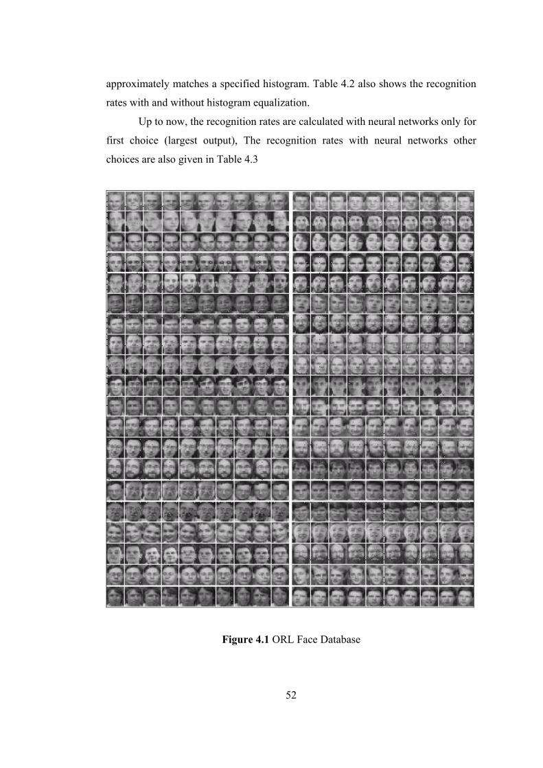
approximately matches a specified histogram. Table 4.2 also shows the recognition

rates with and without histogram equalization.

Up to now, the recognition rates are calculated with neural networks only for

first choice (largest output), The recognition rates with neural networks other

choices are also given in Table 4.3

Figure 4.1 ORL Face Database

52

Figure 4.2 Mean face for ORL Face Database

Figure 4.3 The eigen values for ORL Face Database

53

Figure 4.4 The top 30 eigen faces for the ORL Face Database

Table 4.1 Recognition Rate using different Number of Training and Test

Images, and w/wo Histogram Equalization

Number of Images

used in Training (per individual)

Number of Images

used in Testing (per individual)

Number of Eigenfaces

Hist. Equ.

Recognition Rate (%)

1 9 10 √ 8.8 1 9 10 X 9.7 2 8 20 √ 25 2 8 20 X 26 3 7 25 √ 51.7 3 7 25 X 51.7 4 6 30 √ 75 4 6 30 X 76.2 5 5 50 √ 87.5 5 5 50 X 90 6 4 60 √ 90 6 4 60 X 92.5 7 3 100 √ 89.1 7 3 100 X 91.6 8 2 100 √ 88.8 8 2 100 X 91.2 9 1 100 √ 87.5 9 1 100 X 90

Number of Neurons in Hidden Layer: 15

54

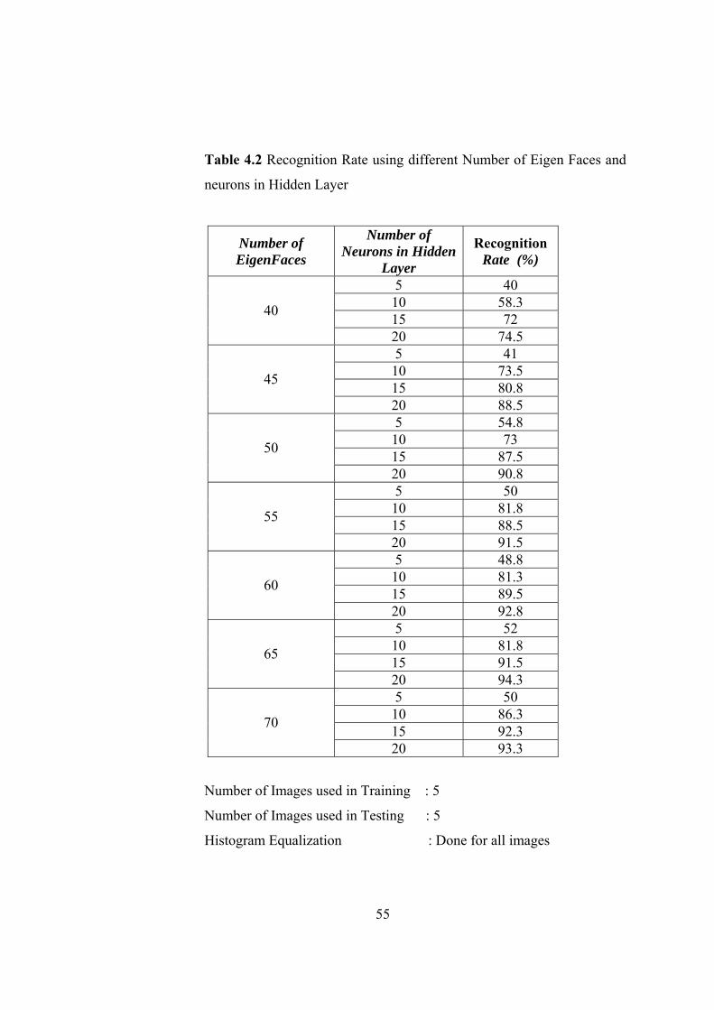
Table 4.2 Recognition Rate using different Number of Eigen Faces and

neurons in Hidden Layer

Number of EigenFaces

Number of Neurons in Hidden

Layer

Recognition Rate (%)

5 40 10 58.3 15 72 40

20 74.5 5 41 10 73.5 15 80.8 45

20 88.5 5 54.8 10 73 15 87.5 50

20 90.8 5 50 10 81.8 15 88.5 55

20 91.5 5 48.8 10 81.3 15 89.5 60

20 92.8 5 52 10 81.8 15 91.5 65

20 94.3 5 50 10 86.3 15 92.3 70

20 93.3

Number of Images used in Training : 5

Number of Images used in Testing : 5

Histogram Equalization : Done for all images

55

Table 4.3 Recognition Rate with Neural Networks different choices

Rank 1 Rank 2 Rank 3 Rank 4 Rank 5

Number of Correct Decision (Over 400 Images) 360 21 7 4 2

Recognition Rate 90% 95.2 % 97% 98% 98.5 %

Number of Testing Images : 5

Number of Eigenfaces : 50

Number of H. L. Neurons : 15

4.2. Test Results for the Olivetti and Oracle Research Laboratory (ORL) Face Database with Eye Extraction

In this section, Eye based recognition is tested on this database. Eyes are

cropped from the faces and then recognition performance is tested only with eyes.

Firstly a rectangular with size 15 x 62 is created (shown in Figure 4.5) and then

eyes are cropped from the faces manually with this rectangle. The mean eye, and

the top 30 (with highest eigenvalues) eigeneyes are shown in Figure 4.6 and Figure

4.7 respectively. The test results and the recognition ratios with different number of

training images and w/wo histogram equalization, and different number of

eigenfaces and neurons in hidden layer are given in Table 4.4 and Table 4.5

respectively. The recognition rates with neural networks first, second, third, forth

and fifth choices are also given in Table 4.6

56

62

15

62

15

Figure 4.5: The eye extraction

Figure 4.6: The mean eye

Figure 4.7: The top 30 Eigeneyes

57

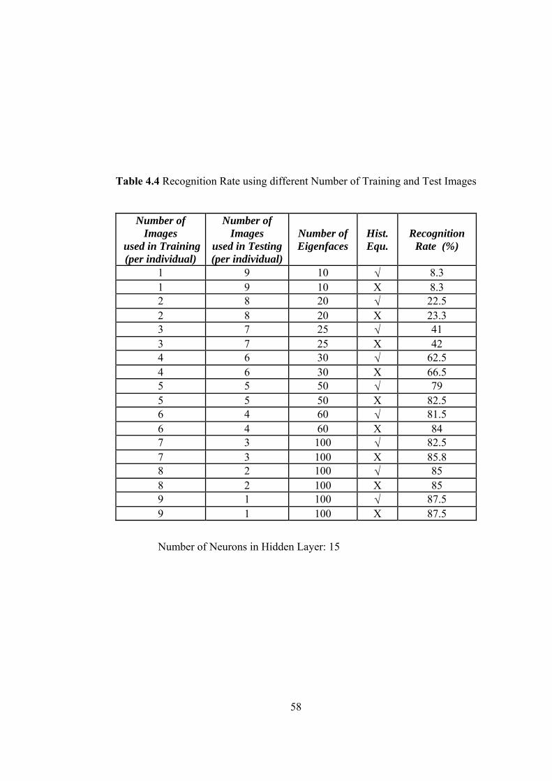
Table 4.4 Recognition Rate using different Number of Training and Test Images

Number of Images

used in Training (per individual)

Number of Images

used in Testing (per individual)

Number of Eigenfaces

Hist. Equ.

Recognition Rate (%)

1 9 10 √ 8.3 1 9 10 X 8.3 2 8 20 √ 22.5 2 8 20 X 23.3 3 7 25 √ 41 3 7 25 X 42 4 6 30 √ 62.5 4 6 30 X 66.5 5 5 50 √ 79 5 5 50 X 82.5 6 4 60 √ 81.5 6 4 60 X 84 7 3 100 √ 82.5 7 3 100 X 85.8 8 2 100 √ 85 8 2 100 X 85 9 1 100 √ 87.5 9 1 100 X 87.5

Number of Neurons in Hidden Layer: 15

58

Table 4.5 Recognition Rate using different Number of Eigen Faces and

neurons in Hidden Layer

Number of EigenFaces

Number of Neurons in Hidden

Layer

Recognition Rate (%)

5 30.5 10 45.5 15 62 40

20 66.5 5 37 10 42 15 68.5 45

20 71.5 5 43.5 10 50.5 15 79 50

20 79 5 47.5 10 54.5 15 79.5 55

20 81 5 48.8 10 63.5 15 81 60

20 84.5 5 44.5 10 61 15 81.5 65

20 80.5 5 50 10 60.5 15 82 70

20 82.5

Number of Images used in Training : 5

Number of Images used in Testing : 5

Histogram Equalization : Done for all images

59

Table 4.6 Recognition Rate with Neural Networks different choices

Rank 1 Rank 2 Rank 3 Rank 4 Rank 5Number of Correct

Decision (Over 400 Images) 330 17 11 5 2

Recognition Rate 82.5 % 86.7 % 89.5% 90% 91.2 %

Number of Testing Images : 5

Number of Eigenfaces : 50

Number of H. L. Neurons : 15

4.3. Test Results for Yale Face Database

The Yale Face Database is used in order to test our method in the presence

of headpose variations. The Yale Face Database contains 165 grayscale images in

GIF format of 15 individuals. There are 11 images per subject, one per different

facial expression or configuration: center-light, w/glasses, happy, left-light, w/no

glasses, normal, right-light, sad, sleepy, surprised, and wink. The whole database is

shown in Figure 4.8.

Since the number of networks is equal to the number of people in the

database, fifteen networks one for each person was created. Within the eleven

images, first 4 of them are used for tanning the neural networks, and then these

networks are tested and updated with the next 3 pictures for getting the minimum

squared error function. And these values will be used for later use for recognition of

the faces.

For testing the whole database, the faces used in training, testing and

recognition are changed and the recognition performance is given for whole

database.

For this database, the mean face of the faces, the calculated top 30 (with

highest eigenvalues) eigenfaces, and their corresponding eigenvalues are shown in

Figure 4.9, Figure 4.10 and Figure 4.11 respectively.

The test results and the recognition ratios with different number of training

images and w/wo histogram equalization, and different number of eigenfaces and

60

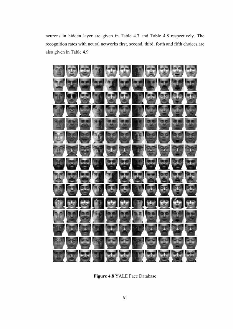
neurons in hidden layer are given in Table 4.7 and Table 4.8 respectively. The

recognition rates with neural networks first, second, third, forth and fifth choices are

also given in Table 4.9

Figure 4.8 YALE Face Database

61

Figure 4.9 Mean face for YALE Face Database

Figure 4.10 The eigen values for ORL Face Database

Figure 4.11 The top 30 eigen faces for the YALE Face Database

62

Table 4.7 Recognition Rate using different Number of Training and Test Images

and with and without Histogram Equalization

Number of Images

used in Training (per individual)

Number of Images

used in Testing (per individual)

Number of Eigenfaces

Hist. Equ.

RecognitionRate (%)

1 10 10 √ 16.6 1 10 10 X 12 2 9 15 √ 37 2 9 15 X 33.3 3 8 30 √ 54.2 3 8 30 X 45.8 4 7 30 √ 75.2 4 7 30 X 71.4 5 6 30 √ 94 5 6 30 X 90.6 6 5 30 √ 93 6 5 30 X 88 7 4 50 √ 91.6 7 4 50 X 86.7 8 3 50 √ 91.1 8 3 50 X 88.8 9 2 50 √ 90 9 2 50 X 90 10 1 50 √ 93.3 10 1 50 X 93.3

Number of Neurons in Hidden Layer: 15

63

Table 4.8 Recognition Rate using different Number of Eigen Faces and

neurons in Hidden Layer

Number of EigenFaces

Number of Neurons in Hidden

Layer

Recognition Rate (%)

5 37 10 53 15 68.5 10

20 81.2 5 35.1 10 71 15 80 15

20 89 5 46 10 74 15 84.2 20

20 90 5 51 10 71 15 78.8 25

20 89 5 53.3 10 80 15 94 30

20 95.1 5 46 10 79.4 15 95.1 35

20 94.5 5 49 10 80 15 92.7 40

20 94

Number of Images used in Training : 5

Number of Images used in Testing : 6

Histogram Equalization : Done for all images

64

Table 4.9 Recognition Rate with Neural Networks different choices

Number of Correct Matches Person Rank 1 Rank 2 Rank 3 Rank 4 Rank 5

1 9 1 1 2 11 3 10 1 4 11 5 11 6 11 7 10 1 8 11 9 10 1

10 9 2 11 11 12 10 1 13 10 1 14 11 15 10 1

Recognition Rate 94% 97.5 % 98.7 % 99.3 % 100%

Number of Testing Images : 5

Number of Eigenfaces : 30

Number of H. L. Neurons : 15

4.4. Test Results for the Yale Face Database with Eye Extraction

In this section eyes are cropped from the faces and then recognition

performance is tested only with eyes. In Yale Database, all pictures have 100x100

dimensions and the left and right eye centers are placed at (30,30) and (70,30)

coordinates respectively. The eye regions are cropped with the rectangle with

dimension 15x68 and centered at the middle coordinates of the eyes. The eye

extraction, the mean eye and the top 30 eigeneyes (with highest eigenvalues) are

shown in Figure 4.12, Figure 4.13, and Figure 4.14 respectively. The test results and

the recognition ratios with different number of training images, eigenfaces and

number of neurons in hidden layer are given in Table 4.10 and Table 4.11

respectively. The recognition rates with neural networks first, second, third, forth

and fifth choices are also given in Table 4.12

65

15

68

(70,30)(30,30)

Figure 4.12 Eye Extraction

Figure 4.13 The YALE Face Database Mean Eye

Figure 4.14 The YALE Face Database Top 30 Eigeneyes

66

Table 4.10 Recognition Rate using different Number of Training and Test Image

Number of

Images used in Training (per individual)

Number of Images

used in Testing (per individual)

Number of Eigenfaces

Hist. Equ.

RecognitionRate (%)

1 10 10 √ 13.3 1 10 10 X 12 2 9 15 √ 33.3 2 9 15 X 30 3 8 30 √ 50 3 8 30 X 46 4 7 30 √ 57.1 4 7 30 X 52.3 5 6 30 √ 69.5 5 6 30 X 64 6 5 30 √ 78 6 5 30 X 70.5 7 4 50 √ 86.5 7 4 50 X 79 8 3 50 √ 87 8 3 50 X 80.5 9 2 50 √ 90 9 2 50 X 76.7 10 1 50 √ 86.7 10 1 50 X 73.3

Number of Neurons in Hidden Layer: 15

67

Table 4.11 Recognition Rate using different Number of Eigen Faces and neurons in Hidden Layer

Number of EigenFaces

Number of Neurons in Hidden

Layer

Recognition Rate (%)

5 35.7 10 51 15 62 10

20 65 5 38 10 49 15 60 15

20 64 5 41 10 61 15 65 20

20 68 5 42 10 64 15 64 25

20 69 5 48.5 10 69 15 69.5 30

20 69.5 5 46 10 70 15 70 35

20 73 5 46 10 68 15 70 40

20 73

Number of Images used in Training : 5

Number of Images used in Testing : 6

Histogram Equalization : Done for all images

68

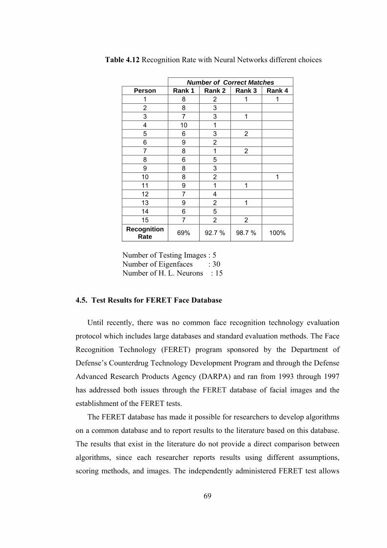
Table 4.12 Recognition Rate with Neural Networks different choices

Number of Correct Matches

Person Rank 1 Rank 2 Rank 3 Rank 4 1 8 2 1 1 2 8 3 3 7 3 1 4 10 1 5 6 3 2 6 9 2 7 8 1 2 8 6 5 9 8 3

10 8 2 1 11 9 1 1 12 7 4 13 9 2 1 14 6 5 15 7 2 2

Recognition Rate 69% 92.7 % 98.7 % 100%

Number of Testing Images : 5 Number of Eigenfaces : 30 Number of H. L. Neurons : 15

4.5. Test Results for FERET Face Database

Until recently, there was no common face recognition technology evaluation

protocol which includes large databases and standard evaluation methods. The Face

Recognition Technology (FERET) program sponsored by the Department of

Defense’s Counterdrug Technology Development Program and through the Defense

Advanced Research Products Agency (DARPA) and ran from 1993 through 1997

has addressed both issues through the FERET database of facial images and the

establishment of the FERET tests.

The FERET database has made it possible for researchers to develop algorithms

on a common database and to report results to the literature based on this database.

The results that exist in the literature do not provide a direct comparison between

algorithms, since each researcher reports results using different assumptions,

scoring methods, and images. The independently administered FERET test allows

69

for a direct quantitative assessment of the relative strengths and weaknesses of

different approaches.

The FERET database released in March 2001, consists of 14051 eight-bit

grayscale images from 1196 individuals. The images are stored in .TIF format and

as raw 8-bit data. They are 256 x 384 (width x height). Attempts were made to keep

the intraocular distance (the distance between the eyes) of each subject to between

40 and 60 pixels. The images consist primarily of an individuals head, neck, and

sometimes the upper part of the shoulders.

The naming convention for the FERET imagery in this distribution is of the

form nnnnnxxfffq_yymmdd.ext where:

1. nnnnn is a five digit integer that uniquely identifies the subject

2. xx is a two lowercase character string that indicates the kind of imagery:

70

Table 4.13. Explanation of Naming Convention

Two Letter code

Pose Angle (degrees) Description

Number in Database

Number of

Subjects Fa 0 = frontal Regular facial expression 1762 1010 Fb 0 Alternative facial expression 1518 1009 ba 0 Frontal “b” series 200 200 bj 0 Alternative expression to ba 200 200 bk 0 Different illumination to ba 200 200 bb +60 200 200 bc +40 200 200 bd +25 200 200 be +15

Subject faces to his left which is the photographer’s right

200 200 bf -15 200 200 bg -25 200 200 Bh -40 200 200 bi -60

Subject faces to his right which is the photographer’s left

200 200 ql -22.5 763 508 qr +22.5

Quarter left and right 763 508 hl -67.5 1246 904 hr +67.5

Half left and right 1298 939 pl -90 1318 974 pr +90

Profile left and right 1342 980 Ra +45 322 264 Rb +10 322 264 Rc -10 613 429 Rd -45 292 238 Re -80

Random images. See note below. Positive angles indicate subject faces to photographer’s right

292 238

Notes:

• fa indicates a regular frontal image

• fb indicates an alternative frontal image, taken seconds after the

corresponding fa

• ba is a frontal images which is entirely analogous to the fa series

• bj is an alternative frontal image, corresponding to a ba image, and

analogous to the fb image

• bk is also a frontal image corresponding to ba, but taken under

different lighting

71

• bb through bi is a series of images taken with the express intention

of investigating pose angle effects (see below). Specifically, bf - bi

are symmetric analogues of bb - be.

• ra through re are “random” orientations. Their precise angle is

unknown. It appears that the pose angles are random but consistent.

The pose angles in the table were derived by manual measurement

of inter-eye distances in the image, and in their corresponding

frontal image.

3. fff is a set of three binary (zero or one) single character flags. In order these

denote:

a. Indicates whether the image is releasable for publication. The flag

has fallen into disuse: All images are available via this CDROM

distribution, but still none may be published without the explicit

written permission of the government. See the restrictions in the

release agreement.

b. Image is histogram adjusted if this flag is 1

c. Indicates whether the image was captured using ASA 200 or 400

film, 0 implies 200.

4. q is a modifier that is not always present. When it is, the meanings are as

follows:

a. Glasses worn. Note that this flag is a sufficient condition only,

images of subjects wearing glasses do not necessarily carry this flag.

Some retroactive re-truthing of such images to fix this problem is

warranted. See also “c” below.

b. Duplicate with different hair length.

c. Glasses worn and different hair length

d. Electronically scaled (resized) and histogram adjusted.

e. Clothing has been electronically retouched.

f. Image brightness has been reduced by 40%

72

g. Image brightness has been reduced by 80%

h. Image size has been reduced by 10%, with white border replacement

i. Image size has been reduced by 20%, with white border replacement

j. Image size has been reduced by 30%, with white border replacement

Note that the modifications d through j are the result of applying various off-

line operations to real images in the database; the “parent” image is that

image without the “q” modifier present at all.

5. The three fields are the date that the picture was taken in year, month, and

day format.

6. The filename extension is .tif. The images on the CDROMs carry an

additional .bz2 suffix that indicates that the files have been losslessly

compressed using the free bzip2 compressor, supplied with the database in

misc/bzip2/.

The FERET tests can be conducted using the gallery (training) and probe (test)

images suggested by the FERET team in the FERET CD-ROM. Table 4.9 shows

the suggested gallery and probe images in the database and which probe names test

which evaluation task. The gallery set is the same for all the four test setups. Such a

suggestion is stated in order to standardize the test results. It is important to point

out here that the gallery and probe sets use only the frontal images which are also

the main concern of this thesis. Also note that the tests used a single gallery

containing 1196 images. The Duplicate I probe images (dup1) were obtained

anywhere between one minute and 1031 days (34 months) after their respective

gallery matches. The harder Duplicate II probe images (dup2) are a strict subset of

the Duplicate I images; they are those taken between 540 and 1031 days (18

months) after their gallery entries. There is usually only a few seconds between the

capture of the gallery-probe pairs in facial expression evaluation probe images

(fafb).

73

Table 4.14: The Gallery and Probe Sets used in the standard FERET test in September 1996.

Evaluation

Task Recognized

Names Gallery (1196)

Probe Set

Aging of subjects Duplicate I gallery.names probe_dup_1_*.names

(722) Aging of subjects Duplicate II gallery.names probe_dup_2_*.names

(234) Facial

Expression fafb gallery.names probe_fafb_*.names (1195)

Different camera and Illumination

fafc gallery.names probe_fafc_*.names (194)

Information about the standard FERET September 1996 gallery and probe sets is

given in Table 4.9. As there is 1 image per individual in the FERET database

standard gallery set, the tests are performed using this set and different gallery and

probe sets constructed using some other criteria. The studied test sets [40] are as

follows;

a) The standard FERET dataset: The files given in the FERET distribution CD of

March 2001 are;

1. gallery.names: contains 1196 images from 1196 individuals.

2. probe_fafb_expression.names: contains 1195 images with alternative

facial expressions.

3. probe_fafc_diffcamera_diffillum.names: contains 194 images taken with

different camera and under different illumination conditions.

4. probe_dup1_temporal_zero_to_34_months.names: contains 722 images

taken at anytime between the one minute and 34 months.

5. probe_dup2_at_least_18_months.names: contains 234 images taken at

anytime between 18 months and 34 months. This set is a subset of the

dup1 set.

74

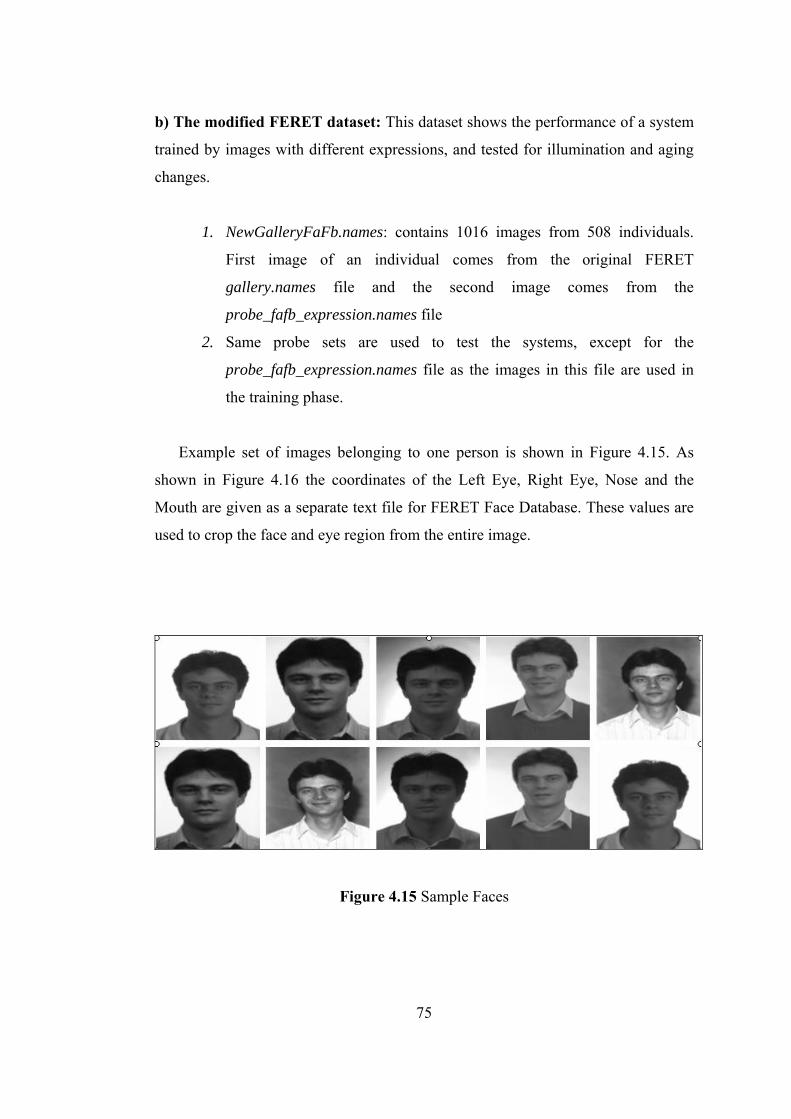
b) The modified FERET dataset: This dataset shows the performance of a system

trained by images with different expressions, and tested for illumination and aging

changes.

1. NewGalleryFaFb.names: contains 1016 images from 508 individuals.

First image of an individual comes from the original FERET

gallery.names file and the second image comes from the

probe_fafb_expression.names file

2. Same probe sets are used to test the systems, except for the

probe_fafb_expression.names file as the images in this file are used in

the training phase.

Example set of images belonging to one person is shown in Figure 4.15. As

shown in Figure 4.16 the coordinates of the Left Eye, Right Eye, Nose and the

Mouth are given as a separate text file for FERET Face Database. These values are

used to crop the face and eye region from the entire image.

Figure 4.15 Sample Faces

75

0

(RightEye_x , RightEye_y) (LeftEye_x , LeftEye_y)

(Nose_x , Nose_y) (Mouth_x , Mouth_y)

384 0 256

Figure 4.16 Sample Face with given coordinates

4.5.1. Preprocessing Stage

The images are preprocessed to improve the recognition performance in this

stage. Firstly tilt compensation is done over the images. When the positions for the

right and left eyes are known, the inverse tangent of the angle between the eye centers

can be calculated. The image can be rotated using the calculated angle. then the

coordinates of the eyes nose and mouth are updated according to tilt compensation

The calculation of the tilt angle is given in Figure 4.19.

The region of the image where the face is located is cut out from the image

and only this area is used in the process of face recognition. The face is cropped from

the entire image with using the Left Eye, Right Eye and the mouth coordinates. The

cropping procedure is shown in Figure 4.20 with the width and the length of the

cropping rectangle specified by means of the coordinates of the faces.

76

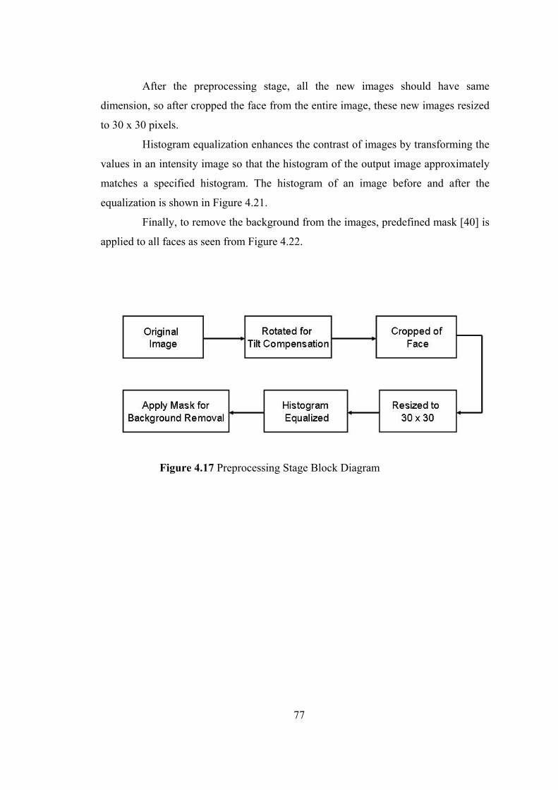
After the preprocessing stage, all the new images should have same

dimension, so after cropped the face from the entire image, these new images resized

to 30 x 30 pixels.

Histogram equalization enhances the contrast of images by transforming the

values in an intensity image so that the histogram of the output image approximately

matches a specified histogram. The histogram of an image before and after the

equalization is shown in Figure 4.21.

Finally, to remove the background from the images, predefined mask [40] is

applied to all faces as seen from Figure 4.22.

Figure 4.17 Preprocessing Stage Block Diagram

77

Face Region Cropped

Resized to 30x30 Rotated to Compensate

Tilt Angle & Coordinates Updated

Histogram Equalized

Masked for Background

Removal

Figure 4.18 Preprocessing Stage

Mid Line

Фtilt

αdy

α

dx

Fig

Фtilt = arctan (dy /dx)

ure 4.19 Tilt Compensation

78

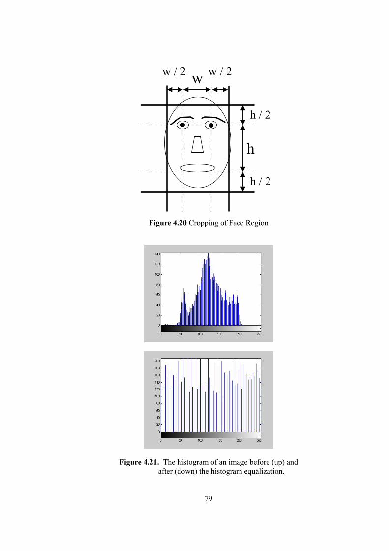
h / 2

h / 2

w w / 2w / 2

h

Figure 4.20 Cropping of Face Region

Figure 4.21. The histogram of an image before (up) and after (down) the histogram equalization.

79

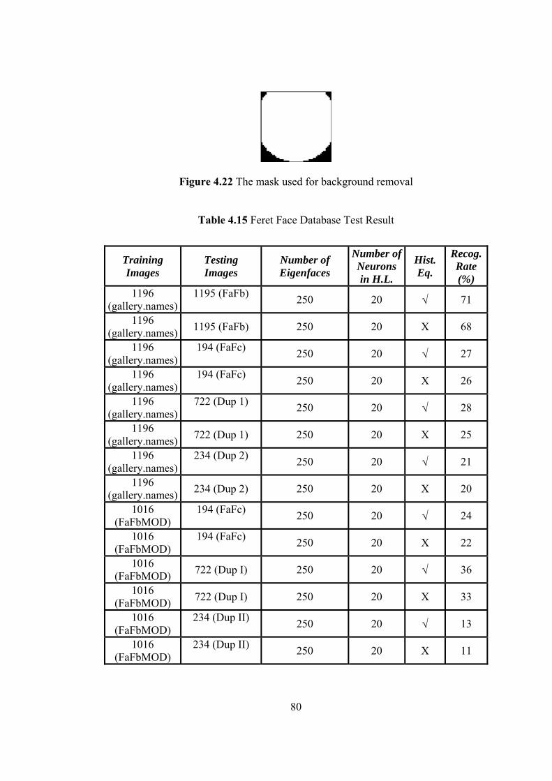
Figure 4.22 The mask used for background removal

Table 4.15 Feret Face Database Test Result

Training Images

Testing Images

Number of Eigenfaces

Number of Neurons in H.L.

Hist. Eq.

Recog. Rate (%)

1196 (gallery.names)

1195 (FaFb) 250 20 √ 71

1196 (gallery.names) 1195 (FaFb) 250 20 X 68

1196 (gallery.names)

194 (FaFc) 250 20 √ 27

1196 (gallery.names)

194 (FaFc) 250 20 X 26

1196 (gallery.names)

722 (Dup 1) 250 20 √ 28

1196 (gallery.names) 722 (Dup 1) 250 20 X 25

1196 (gallery.names)

234 (Dup 2) 250 20 √ 21

1196 (gallery.names) 234 (Dup 2) 250 20 X 20

1016 (FaFbMOD)

194 (FaFc) 250 20 √ 24

1016 (FaFbMOD)

194 (FaFc) 250 20 X 22

1016 (FaFbMOD) 722 (Dup I) 250 20 √ 36

1016 (FaFbMOD) 722 (Dup I) 250 20 X 33

1016 (FaFbMOD)

234 (Dup II) 250 20 √ 13

1016 (FaFbMOD)

234 (Dup II) 250 20 X 11

80

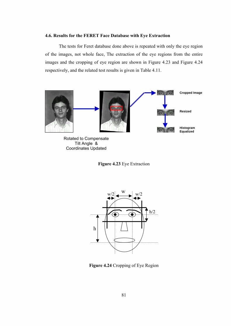
4.6. Results for the FERET Face Database with Eye Extraction The tests for Feret database done above is repeated with only the eye region

of the images, not whole face, The extraction of the eye regions from the entire

images and the cropping of eye region are shown in Figure 4.23 and Figure 4.24

respectively, and the related test results is given in Table 4.11.

Cropped Image

Resized

Histogram Equalized

Rotated to Compensate Tilt Angle &

Coordinates Updated

Figure 4.23 Eye Extraction

h/2

h

ww/2 w/2

Figure 4.24 Cropping of Eye Region

81

Table 4.16 Feret Face Database Tets Results with Eye Extraction

Training Images

Testing Images

Number of Eigenfaces

Number of Neurons in H.L.

Hist. Eq.

Recog. Rate (%)

1196 (gallery.names)

1195 (FaFb) 250 20 √ 54

1196 (gallery.names) 1195 (FaFb) 250 20 X 51

1196 (gallery.names)

194 (FaFc) 250 20 √ 17

1196 (gallery.names)

194 (FaFc) 250 20 X 14

1196 (gallery.names)

722 (Dup 1) 250 20 √ 19

1196 (gallery.names) 722 (Dup 1) 250 20 X 17

1196 (gallery.names)

234 (Dup 2) 250 20 √ 20

1196 (gallery.names) 234 (Dup 2) 250 20 X 18

1016 (FaFbMOD)

194 (FaFc) 250 20 √ 19

1016 (FaFbMOD)

194 (FaFc) 250 20 X 17

1016 (FaFbMOD) 722 (Dup I) 250 20 √ 29

1016 (FaFbMOD) 722 (Dup I) 250 20 X 25

1016 (FaFbMOD)

234 (Dup II) 250 20 √ 12

1016 (FaFbMOD)

234 (Dup II) 250 20 X 11

82

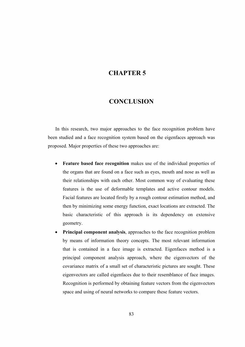
CHAPTER 5

CONCLUSION

In this research, two major approaches to the face recognition problem have

been studied and a face recognition system based on the eigenfaces approach was

proposed. Major properties of these two approaches are:

• Feature based face recognition makes use of the individual properties of

the organs that are found on a face such as eyes, mouth and nose as well as

their relationships with each other. Most common way of evaluating these

features is the use of deformable templates and active contour models.

Facial features are located firstly by a rough contour estimation method, and

then by minimizing some energy function, exact locations are extracted. The

basic characteristic of this approach is its dependency on extensive

geometry.

• Principal component analysis, approaches to the face recognition problem

by means of information theory concepts. The most relevant information

that is contained in a face image is extracted. Eigenfaces method is a

principal component analysis approach, where the eigenvectors of the

covariance matrix of a small set of characteristic pictures are sought. These

eigenvectors are called eigenfaces due to their resemblance of face images.

Recognition is performed by obtaining feature vectors from the eigenvectors

space and using of neural networks to compare these feature vectors.

83

Eigenfaces based approach excels in its speed, simplicity and learning

capability.

A robust face recognition system should be insensitive to

• Changes in illumination,

• Changes in head orientation and scale,

• Presence of facial details such as glasses, beards,

• Face background.

With the principal component analysis method, face authentication, based on

face and only eye region is implemented. Experimental results have shown that, the

proposed face recognition method was very sensitive to face background and head

orientations. Changes in the illumination did not cause a major problem to the

system.

Proposed method is applied on three different databases, ORL (Olivetti

Research Laboratory) Database, Yale Database and FERET (Face Recognition

Technology) Database.

Firstly ORL face database is used for tests. In this database there are 10

different images of each of 40 distinct subjects. The recognition rates, with different

number of eigenfaces and hidden layer neurons in neural network system are

implemented. It is found that for the whole database, 5 training images per person,

50 eigenface for total database and 15 neurons in hidden layer are enough for

satisfactory recognition rates (about 90 %). The eigenface method is very sensitive to

head orientations, and the mismatches occur for the images with large head

orientations. After these tests, the eye region are cropped from all of the images, and

tests are repeated for authentication of the faces based on eye region and see that the

authentication performance decreases but still remains satisfactory (about 93 %).

Again the mismatches occur when there are large head orientations and when the

eyes of the person are closed. The recognition results for this database are compared

with the early techniques and the results are given in Table 5.1.

84

Table 5.1 Performance results for ORL Face Database

Method Recognition Rate (%)

Elastic Graph Mapping 80

Line Based 97

LDA 80

Bayesian PCA 93

Proposed Method 93

Then the tests are repeated for Yale Face Database. This database is used in

order to test our method in the presence of headpose variations. There are 15

different people with 11 images per subject, one per different facial expression or

configuration. We get better recognition results for Yale database (about 95 %)

because eigenface method is less sensitive to illumination changes and presence of

small details than head orientations. Then eye regions are cropped from all images

and the tests are repeated. We see that the recognition performance decreased

slightly. Since the authentication is implemented only with eye region, especially

images of person wearing glasses, or with closed eyes causes mismatches in these

tests. Recognition results for this database with early techniques [41] are given in

Table 5.2.

Table 5.2 Performance results for Yale Database

Method Recognition Rate (%)

Euclidean Distance 60

Template Matching 85

Proposed Method 95

85

FERET database is the final database used during simulations. There is one

image per individual in the standard FERET training set, one more modification of

the standard FERET subset is also produced for the tests. The recognition rates for

the FERET database is much less than for the ORL and Yale databases, because

there is just one training image per person in standard, and just two training images

per person in modified FERET database. Recognition results for this database with

early techniques [39] are given in Table 5.3.

Arl_cor is a normalized correlation based algorithm For normalized

correlation, the images were (1) translated, rotated, and scaled so that the center of

the eyes were placed on specific pixels and (2) faces were masked to remove

background and hair. Arl_ef is a principal components analysis (PCA) based

algorithm These algorithms are developed by U.S. Army Research Laboratory

and they provide a performance baseline. In the implementation of the PCA-based

algorithm, all images were (1) translated, rotated, and scaled so that the center

of the eyes were placed on specific pixels, (2) faces were masked to remove

background and hair, and (3) the non-masked facial pixels were processed by a

histogram equalization algorithm. The training set consisted of 500 faces.

Faces were represented by their projection onto the first 200 eigenvectors and

were identified by a nearest neighbor classifier using the L1

metric.ef_hist_dev_ang, ef_hist_dev_anm, ef_hist_dev_l1, ef_hist_dev_l2,

ef_hist_dev_md, ef_hist_dev_ml1, ef_hist_dev_ml2 are seven eigenface based

system from National Institute of Standards and Technology (NIST) with a

common image processing front end and eigenface representation but differing in

the distance metric. Algorithms are also tested from Excalibur Corp. (Carlsbad,

CA), and from University of Maryland (umd_mar_97). There are two algorithms

developed by MIT Media Laboratory using a version of eigenface transform;

mit_mar_95 is the algorithm is the same algorithm that was tested in March

1995, algorithm retested in order to measure improvements, and mit_sep_96 is

the algorithm developed since March 1995. And finally the usc_mar_97 is an

elastic graph matching algorithm from Southern California University.

86

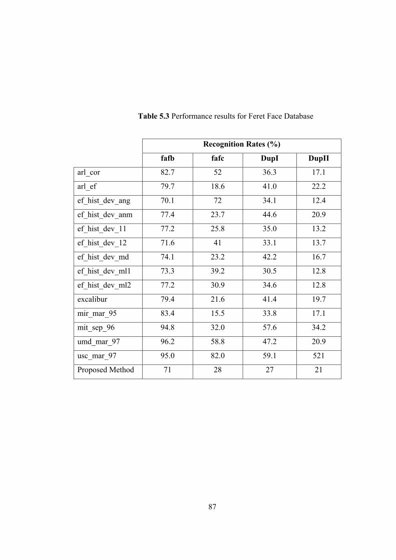
Table 5.3 Performance results for Feret Face Database

Recognition Rates (%)

fafb fafc DupI DupII

arl_cor 82.7 52 36.3 17.1

arl_ef 79.7 18.6 41.0 22.2

ef_hist_dev_ang 70.1 72 34.1 12.4

ef_hist_dev_anm 77.4 23.7 44.6 20.9

ef_hist_dev_11 77.2 25.8 35.0 13.2

ef_hist_dev_12 71.6 41 33.1 13.7

ef_hist_dev_md 74.1 23.2 42.2 16.7

ef_hist_dev_ml1 73.3 39.2 30.5 12.8

ef_hist_dev_ml2 77.2 30.9 34.6 12.8

excalibur 79.4 21.6 41.4 19.7

mir_mar_95 83.4 15.5 33.8 17.1

mit_sep_96 94.8 32.0 57.6 34.2

umd_mar_97 96.2 58.8 47.2 20.9

usc_mar_97 95.0 82.0 59.1 521

Proposed Method 71 28 27 21

87

REFERENCES

[1] F.Galton, “Personal identification and description 1,1 Nature, pp.173-177,21

June1988

[2] Sir Francis Galton, Personal identification and description-II”, Nature 201-

203, 28 June 1988

[3] Goldstein, A. J., Harmon, L. D., and Lesk, A. B., Identification of human

faces", Proc. IEEE 59, pp. 748-760, (1971).

[4] Haig, N. K., "How faces differ - a new comparative technique", Perception

14, pp. 601-615, (1985).

[5] Rhodes, G., "Looking at faces: First-order and second order features as

determinants of facial appearance", Perception 17, pp. 43-63, (1988).

[6] Kirby, M., and Sirovich, L., "Application of the Karhunen-Loeve procedure for

the characterization of human faces", IEEE PAMI, Vol. 12, pp. 103-108,

(1990).

[7] Sirovich, L., and Kirby, M., "Low-dimensional procedure for the

characterization of human faces", J. Opt. Soc. Am. A, 4, 3, pp. 519-524,

(1987).

[8] Terzopoulos, D., and Waters, K., "Analysis of facial images using physical

and anatomical models", Proc. 3rd Int. Conf. on Computer Vision, pp. 727-

732, (1990).

[9] Manjunath, B. S., Chellappa, R., and Malsburg, C., "A feature based

approach to face recognition", Trans. of IEEE, pp. 373-378, (1992).

[10] Harmon, L. D., and Hunt, W. F., "Automatic recognition of human face

profiles", Computer Graphics and Image Processing, Vol. 6, pp. 135-156,

(1977).

88

[11] Harmon, L. D., Khan, M. K., Lasch, R., and Ramig, P. F., "Machine

identification of human faces", Pattern Recognition, Vol. 13(2), pp. 97-

110,(1981).

[12] Kaufman, G. J., and Breeding, K. J, "The automatic recognition of human

faces from profile silhouettes", IEEE Trans. Syst. Man Cybern., Vol. 6, pp.

113-120, (1976).

[13] Wu, C. J., and Huang, J. S., "Human face profile recognition by computer",

Pattern Recognition, Vol. 23(3/4), pp. 255-259, (1990).

[14] Kerin, M. A., and Stonham, T. J., "Face recognition using a digital neural

network with self-organizing capabilities", Proc. 10th Int. Conf. On Pattern

Recognition, pp.738-741, (1990).

[15] Nakamura, O., Mathur, S., and Minami, T., "Identification of human faces

based on isodensity maps", Pattern Recognition, Vol. 24(3), pp. 263-272,

(1991).

[16] Turk, M., and Pentland, A., "Eigenfaces for recognition", Journal of

Cognitive Neuroscience, Vol. 3, pp. 71-86, (1991).

[17] Yuille, A. L., Cohen, D. S., and Hallinan, P. W., "Feature extraction from

faces using deformable templates", Proc. of CVPR, (1989).

[18] P.Philips, “The FERET database and evaluation procedure for face

recognition algorithms, “ Image and Vision Computing, vol.16, no.5,

pp.295-306, 1998

[19] D. Sidlauskas, “HAND: give me five,” IEEE Spectrum, pp. 24-25, February

1994.

[20] R.C. Fowler, “FINGERPRINT: an old touchstone decriminalized,” IEEE

Spectrum, pp.26, February 1994.

[21] J.E. Siedlarz, “IRIS:more detailed than a fingerprint,” IEEE spectrum,

pp.27,February 1994.

[22] R.Manddelbaum, “SPEECH: just say the word, “IEEE Spectrum, page 30,

February 1994.

[23] Carey, S., and Diamond, R., "From piecemeal to configurational

representation of faces", Science 195, pp. 312-313, (1977).

89

[24] Bledsoe, W. W., "The model method in facial recognition", Panoramic

Research Inc. Palo Alto, CA, Rep. PRI:15, (August 1966).

[25] Bledsoe, W. W., "Man-machine facial recognition", Panoramic Research

Inc. Palo Alto, CA, Rep. PRI:22, (August 1966).

[26] Fischler, M. A., and Elschlager, R. A., "The representation and matching of

pictorial structures", IEEE Trans. on Computers, c-22.1, (1973).

[27] Yuille, A. L., Cohen, D. S., and Hallinan, P. W., "Feature extraction from

faces using deformable templates", Proc. of CVPR, (1989).

[28] Kohonen, T., "Self-organization and associative memory", Berlin: Springer-

Verlag, (1989).

[29] Kohonen, T., and Lehtio, P., "Storage and processing of information in

distributed associative memory systems", (1981).

[30] Fleming, M., and Cottrell, G., "Categorization of faces using unsupervised

feature extraction", Proc. of IJCNN, Vol. 90(2), (1990).

[31] Kanade, T., "Picture processing system by computer complex and

recognition of human faces", Dept. of Information Science, Kyoto

University, (1973).

[32] Burt, P., "Smart sensing within a Pyramid Vision Machine", Proc. of IEEE,

Vol. 76(8), pp. 139-153, (1988).

[33] Ching, C. W., and Huang, L. C., "Human face recognition from a single

front view", Int. J. of Pattern Recognition and Artificial Intelligence,

Vol. 6(4), pp. 570-593, (1992).

[34] Berger, M. O., and Mohr, R., "Towards autonomy in active contour models",

Proc. 10th Int. Conf. on Pattern Recognition, pp. 847-851, (1990).

[35] Kass, M., Witkin, A., and Terzopoulos, D., "Snakes: Active contour

models", Int. J. of Computer Vision, pp. 321-331, (1987).

[36] Williams, D. J., and Shah, M., "A fast algorithm for active contours", Proc.

3rd Int. Conf. on Computer Vision, pp. 592-595, (1990).

[37] Amir, A. A., Weymouth, T. E., and Jain, R. C., "Using dynamic

programming for solving variational problems in vision", IEEE PAMI, Vol.

12(9), pp. 855-867, (1990).

90

[38] Press, W. H., Flannery, B. P., Teukolsky, S. A., Vetterling, W. T., "Numerical

recipes in C", Cambridge University Press, pp. 353-380, (1988).

[39] B. Kepenekci, “Face Recognition Using Gabor Wavelet Transform”, MSc.

Thesis, METU, September 2001.

[40] A.Bahtiyar Gül, “ Holistic Face Recognition By Dimension Reduction”, MSc

Thesis, METU, September 2003

[41] E. DEDE, “Face Recognition Using Geometric Features and Template

Matching By Dimension Reduction”, MSc Thesis, METU, September 2003

91