Face Detection using Hierarchical SVM ECE 795 – Pattern Recognition

Christos Kyrkou

Fall Semester 2010

2

1. Introduction

Face detection in video is the process of detecting and classifying small images extracted

from a sequence of video frames as face or not a face [1]. This can be achieved by applying pattern recognition algorithms. Face detection has been applied in image and video data mining applications that span from security and bioinformatics, to human-computer-interaction, and facial expression analysis. The process of face detection involves locating the image regions that contain an object of interest in the input video frame, regardless of the varying features of the object. This is done by examining usually small frame regions called search windows of m x n pixels. These search windows are generated from the original source image and the classification algorithm is applied to each window. An object detection system typically consists of three stages. The first is the image pyramid generation stage. The second stage includes any enhancements that improve the quality of the search windows, and the third stage involves the classification stage, which is the stage which is the main focus of this project.

There are many algorithms in literature that have been used in the context of face detection but the most successful ones are based on artificial neural networks (ANNs) [2], and the newly introduced Viola-Jones detection framework which is based on Haar-Features [3].Recently support vector machines (SVMs) have also attracted interest from the computer vision community as a possible classification algorithm for face detection and object detection in general [4-8]. However, the main drawback of SVMs with respect to the other algorithms is the amount of data that need to process that makes them slow and thus not suitable for real-time applications.

The purpose of this project is to implement a face detection system based on hierarchical support vector machines in order to improve the performance of support vector machines for face detection. The idea of hierarchical classification stages was first proposed in [6], where stages of classifiers each with increased complexity were used so that non promising regions are discarded early in the detection process so that most of the computational time is spent working on promising image regions. The background algorithms and methodology are detailed in Section 2. Experimental results for the detection accuracy and performance are given in Section 3, while Section 4 concludes the project report.

3

2. Background & Methodology

2.1. Face Detection

The process of face detection involves detecting human faces in digital images/video frames. It is considered a complicated problem because of the variability in the appearance of human faces (size, orientation, environmental conditions, etc.). Face detection techniques that use learning algorithms to capture the appearance model of a face are called appearance-based methods [1]. Such algorithms typically perform three tasks in order to perform the detection (Fig. 1), but the methods used for each task may vary between algorithms. Typically the detection is done on a search window which is usually an mxn pixel region of the image.

The first task is the image pyramid generation (IPG) and its purpose is to ensure that face regions larger than the search window will eventually be processed by the classification engine. Two methods can be used to achieve this. The first one is using a scaling factor S to downscale the source image until it reaches the size of the search window. Each pixel in the source image, with coordinates (X,Y) is mapped to new coordinates (X’,Y’) using (1). Each downscaled version is scanned for possible face regions. The second method involves enlarging the search window, up to the maximum possible size depending on the source image dimensions, to cover a wider area. The source image remains as is and each upscaled version of the search window is used to scan the image. Certain tradeoffs are associated with each method regarding detection accuracy, performance and the classification engine design. Concerning the detection accuracy, using the first method will result in loss of information depending on the downscaling algorithm. A better scaling algorithm will preserve more information but will require more computational power. The second method however, does not result in any data loss since the source image information is preserved. The number of downscaled images that are created by the first method impact the overall system performance as it increases the number of generated windows, increasing processing time per source image. Finally, for the first method the classification engine need not be concerned about the number of downscaled versions and only need to process search windows of the same size. Whereas increasing the search window size will require a classification engine capable of processing all possible window sizes, increasing the processing resources demands.

(1)

The second task is the image preprocessing stage, used to filter out noise, lighting, and pose variations in the region of interest. This increases the probability of accurate detection by removing any in class variability, and presents a uniform sample to the classifier.

Fig. 1. Face Detection Process

4

Frequently used preprocessing techniques include Brightness Adjustment, Contrast Adjustment and Histogram Equalization. The preprocessing method is determined by the operating environment. The processing time required for each input image may vary according to the IPG method used. When downscaling the source image the processing time required for each window remains constant, whereas when scaling up the window it will increase as the window size increases.

The third and final task is the detection stage in which the classification engine processes the input search window and outputs the classification result. Performance and detection accuracy are the two important factors when considering a classification engine. The detection accuracy is determined during the training of the classification engine and depends heavily on the training set, and the training algorithm’s generalization capabilities (training method and constraints).

2.2. Methodology

The SVM face detection system implemented in this project is based on a 2 stage hierarchical SVM (first stage is a linear SVM, second stage is a 2nd degree polynomial) that operates on grayscale images with a window size of 19x19 pixels.

Hierarchical SVM

The idea of using hierarchical SVMs to speed up their classification speed was first proposed in [6]. A hierarchical SVM combines linear SVMs with non-linear SVMs in stages to reduce the processing time needed to classify a single input. The advantage of using a linear SVM is that the input need not be processed by all support vectors but only by the feature vector w (which is computed from (2)). However, for non-linear SVMs obtaining the feature vector w is not practical as we need to transform the support vectors into the feature space Φ (.) which is not always known due to the use of kernels. In [6], the final stage is a non-linear SVM (2nd degree polynomial) while previous stages are linear SVMs. The most popular kernels used for non-linear SVMs are the 2nd and 3d degree polynomials due to their reduced complexity compared to RBF kernels [4, 7]. An illustration of the operation of a hierarchical SVM is shown in Fig. 2.

Due to the combination of different models hierarchical SVMs, introduce a trade-off between the detection accuracy and performance. Linear SVMs do not have the discrimination capabilities of the more complex non-linear SVM models there is bound to be some an increase in misclassification rate. As such the linear classification stages must be chosen appropriately in order to reject as less true positives (face regions) as possible while rejecting as many true negatives (non-face regions) as possible. On the other hand linear SVMs have a lower cost, in terms of detection speed, at classifying new input data than non-linear SVMs.

(2) Linear SVM (3)Non-linear SVM

. . .FaceClass

FaceClass

FaceClass

AcceptFace

RejectNon-Face

Non-FaceClass

Non-FaceClass

Non-FaceClass

InputWindow

Fig. 2. Hierarchical SVM Detection Procedure

5

Preprocessing

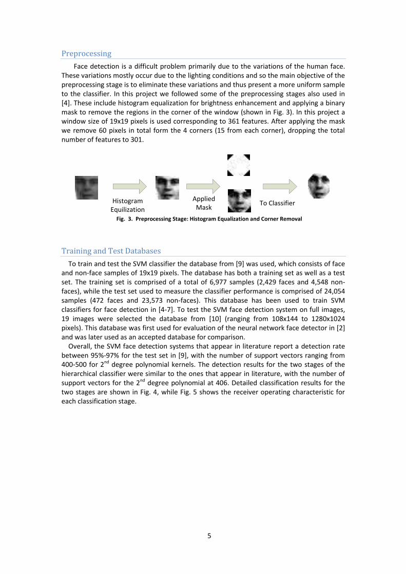
Face detection is a difficult problem primarily due to the variations of the human face. These variations mostly occur due to the lighting conditions and so the main objective of the preprocessing stage is to eliminate these variations and thus present a more uniform sample to the classifier. In this project we followed some of the preprocessing stages also used in [4]. These include histogram equalization for brightness enhancement and applying a binary mask to remove the regions in the corner of the window (shown in Fig. 3). In this project a window size of 19x19 pixels is used corresponding to 361 features. After applying the mask we remove 60 pixels in total form the 4 corners (15 from each corner), dropping the total number of features to 301.

HistogramEquilization

AppliedMask

To Classifier

Fig. 3. Preprocessing Stage: Histogram Equalization and Corner Removal

Training and Test Databases

To train and test the SVM classifier the database from [9] was used, which consists of face and non-face samples of 19x19 pixels. The database has both a training set as well as a test set. The training set is comprised of a total of 6,977 samples (2,429 faces and 4,548 non-faces), while the test set used to measure the classifier performance is comprised of 24,054 samples (472 faces and 23,573 non-faces). This database has been used to train SVM classifiers for face detection in [4-7]. To test the SVM face detection system on full images, 19 images were selected the database from [10] (ranging from 108x144 to 1280x1024 pixels). This database was first used for evaluation of the neural network face detector in [2] and was later used as an accepted database for comparison.

Overall, the SVM face detection systems that appear in literature report a detection rate between 95%-97% for the test set in [9], with the number of support vectors ranging from 400-500 for 2nd degree polynomial kernels. The detection results for the two stages of the hierarchical classifier were similar to the ones that appear in literature, with the number of support vectors for the 2nd degree polynomial at 406. Detailed classification results for the two stages are shown in Fig. 4, while Fig. 5 shows the receiver operating characteristic for each classification stage.

6

Total Correct Detections: 21822 Correct Detections Percentage: 90.755% Total False Detections: 2223 False Detections Percentage: 9.245% Positive: 1 | Negative: -1 Number of Misclassified Samples Positive Class: 214 Number of Misclassified Samples Negative Class: 2009 True Positive Rate: 54.661% False Positive Rate: 8.522% False Negative Rate: 45.339% True Negative Rate: 91.478%

Total Correct Detections: 23519 Correct Detections Percentage: 97.812% Total False Detections: 526 False Detections Percentage: 2.188% Positive: 1 | Negative: -1 Number of Misclassified Samples Positive Class: 331 Number of Misclassified Samples Negative Class: 195 True Positive Rate: 29.873% False Positive Rate: 0.827% False Negative Rate: 70.127% True Negative Rate: 99.173%

(a) (b) Fig. 4. (a) Classification Results on the test set for the linear SVM. (b) Classification Results on the

test set curve for the polynomial SVM.

(a) (b)

Fig. 5. (a) Receiver Operating Characteristic curve for the linear SVM. (b) Receiver Operating Characteristic curve for the polynomial SVM.

7

3. Results & Discussion

3.1. Detection and Performance Results

Comparison of the detection results for each stage and the combination of the two stages is given in Table II. Notice that the non-overlapping regions between the two stages do not remain in the final classification outcome.

Table I: Detection Results for the linear, polynomial and hierarchichal SVM

Linear SVM Detections Polynomial SVM Detections Hierarchichal SVM Detections

1.

2.

3.

4.

8

5.

6.

7.

8.

9.

10.

9

11.

12.

13.

14.

10

15.

16.

17.

18.

11

19.

3.2. Performance Comparison

The performance of the hierarchical SVM is compared with that of a single polynomial SVM to measure the speedup from adding a linear SVM at the preceding stages. Table III shows the time (in seconds) needed to classify the corresponding image for the polynomial and hierarchical SVM, and also the performance speedup from using a hierarchical SVM over the polynomial SVM.

Table II: Performance Speedup of Hierarchical SVM over polynomial

Image Number

Single Polynomial SVM

Performance (seconds)

Hierarchical SVM Performance

(seconds)

Speedup (Polynomial/ Hierarchical)

1. 277.98 90.0781 3.0860

2. 55.57 17.2969 3.2132

3. 40.98 10.2656 3.9924

4. 83.56 22.1719 3.7689

5. 79.53 26.9219 2.9541

6. 10.82 2.6250 4.1250

7. 453.45 187.2969 2.4210

8. 46.32 11.1563 4.1527

9. 80.31 30.3594 2.6454

10. 33.40 9.2344 3.6176

11. 38.92 9.2969 4.1866

12. 85.07 28.5469 2.9803

13. 26.87 7.9688 3.3725

14. 126.65 41.9375 3.0201

15. 18.23 8.6094 2.1180

16. 83.78 25.9375 3.2301

17. 81.78 25.8750 3.1407

18. 57.45 19.3594 2.9677

19. 3.57 1.3438 2.6628

12

3.3. Discussion

An object detection system is characterized by how accurate it can classify data as well as how many image frames it can process per second. The two performance metrics are the detection accuracy, and frames per second or frame rate (FPS). Detection accuracy is usually measured on a given test set where the expected outcome for a sample is compared to the actual outcome of the object detection system. The detection accuracy is the percentage of samples for which the expected outcome matches the actual outcome of the detection system. FPS concerns the throughput of a system and is the maximum number of digital video/image frames, of a given size, that the detection system can process in one second.

The first stage of the hierarchical SVM (linear SVM) manages to find most of the faces in the image but with an increased number of false positives. On the other hand, the polynomial SVM can detect less faces that the linear SVM, but also has a reduced number of false positives. The combination of the two in a hierarchy is a trade-off between the true positive rate of the linear SVM and the false positive rate of the polynomial SVM. We also observe that are not detected by the standalone polynomial SVM will not be detected by the hierarchical SVM either. The linear SVM appears to have a better performance in detecting faces that the polynomial, thus to improve the detection performance of the hierarchical SVM we need only improve the later stage which is the polynomial SVM.

The second performance metric is the time needed to process a single frame. The performance of the polynomial SVM increases with the size of the image. However, this is not always true for the hierarchical SVM. This happens because for a smaller image containing a lot of faces the hierarchical SVM (assuming that it detects the faces correctly) will go through the polynomial SVM many times, thus, increasing the time needed to process the image. However, for a larger image containing no faces, the polynomial SVM may never be utilized (again assuming that the detections correspond to the true class), and so only the linear SVM will be used for classification. From Table III it can be observed that the time that the hierarchical SVM needs to process a single image is always smaller than that of the polynomial SVM which is what was expected from adopting the hierarchical approach. Furthermore, the observed speedup is for all cases more than 2, which indicated that using the hierarchical approach more than doubles the processing speed of an SVM-based face detector with only a small penalty in the detection accuracy with respect to the standalone polynomial.

4. Concluding Remarks

Support vector machines (SVMs) have gained a considerable interest in the past few years from researches as a possible classification step for the problem of face detection. However, the number of support vectors makes SVMs a not so desirable choice when it comes to real time applications. This project concerned the realization of a hierarchical SVM for face detection in order to improve the processing time of SVMs. The face detection system was comprised of a preprocessing stage and a two stage SVM hierarchy (a linear and polynomial SVM). The detection accuracy of the hierarchical SVM is similar to that of a standalone polynomial kernel with some reduction in the true and false positive rate which was expected due to the introduction of the linear kernel. The speedup from using the hierarchical SVM is more than double for all test cases. In conclusion, the results indicate that the use of hierarchical SVM is beneficial and can offer significant improvements when it comes to performance, while maintaining the same detection accuracies as standalone SVMs.

13

5. References

[1] Ming-Hsuan Yang, D. J. Kriegman, N. Ahuja, “Detecting faces in images: a survey,” IEEE

Transactions on Pattern Analysis and Machine Intelligence In Pattern Analysis and Machine Intelligence, IEEE Transactions on, Vol. 24, No. 1. (07 Jan 2002), pp. 34-58.

[2] H. A. Rowley, S. Baluja, and T. Kanade, "Neural network-based face detection," IEEE Transactions on Pattern Analysis and Machine Intelligence, vol. 20, no. 1, pp. 23-38, 1998.

[3] P. Viola and M. Jones, "Robust real-time object detection," in International Journal of Computer Vision, 2001.

[4] E. Osuna, R. Freund, and F. Girosi, “Training support vector machines: an application to face detection,” IEEE Conference on Computer Vision and Pattern Recognition, 1997, pp. 130-136.

[5] H. Sahbi, D. Geman and N. Boujemaa, "Face detection using coarse-to-fine support vector classifiers," International Conference on Image Processing, 2002, pp. 925-928.

[6] B. Heisele, T. Serre, S. Prentice, and T. Poggio. Hierarchical Classification and Feature Reduction for Fast Face Detection with Support Vector Machines. Pattern Recognition, Vol. 36, No. 9, 2007-2017, 2003.

[7] B. Heisele, T. Poggio, M. Pontil, " Face Detection in Still GrayImages," unpublished.

[8] Shavers C., Li R., Lebby G., "An SVM-based approach to face detection," Proceeding of the Thirty-Eighth Southeastern Symposium on System Theory, 2006. SSST '06. , pp.362-366, 5-7 March 2006.

[9] MIT Center for Biological and Computation Learning, “CBCL Face Database #1”, Jan 2010. [Online]. Available: http://cbcl.mit.edu/software-datasets/FaceData2.html

[10] “CMU and MIT Face Database”, Jan 2010. [Online]. Available: http://vasc.ri.cmu.edu/idb/html/face/frontal_images/