1

f(R) THEORIES OF GRAVITY

AND DARK ENERGY

Nathalie Deruelle

APC, Paris

Cargese, Novembre 2008

2

INTRODUCTION

The observed universe is well represented by a Friedmann-Lemaıtre spacetimethe scale factor of which started to accelerate recently

No Big Bang

1 2 0 1 2 3

expands forever

-1

0

1

2

3

2

3

closed

recollapses eventually

Supernovae

CMB

Clusters

open

flat

Knop et al. (2003)Spergel et al. (2003)Allen et al. (2002)

Supernova Cosmology Project

Ω

ΩΛ

M

ds2 = gijdxidxj = −dt2 + a2(t)dσ2k

Gij = κT totalij ; DjT

ij = 0

H2 + ka2 = κ

3ρtotal ; H = 1a

dadt(

HH0

)2

= Ω0rad

(a0a

)4 + Ω0mat

(a0a

)3 + Ω0k

(a0a

)2 + Ω0Λ

H0 ≈ 70 ; Ω0rad ≈ 10−4 ; Ω0

mat ≈ 0.3 , Ω0k ≈ 0

Ω0Λ ≈ 0.7 : Dark Energy

=⇒ κTΛij = −Λgij , a(t)→ e

√Λ/3 t , Λ = 3Ω0

ΛH20

3

Origin of this acceleration

• An artefact of the averaging process ?

Gij(<gkl>) = κ <Tij > instead of <Gij(gkl)>= κ <Tij ><gkl>6= gkl (See Rasanen)

• Exotic matter ? (ρΛ + pΛ ≈ 0)

– Chaplygin gas : pρ = −A, (See Moschella)– Quintessence : R.G. plus ϕ with V ∝ 1/ϕn (See Martin)

• “Modified” gravity ?

– Λ : (See Bernardeau)– MOND (See Combes, Esposito-Farese)– “Branes” : (See Deffayet)– f(R) lagrangian, instead of Hilbert’s R (simpler than f(Ri

jkl) !)C.D.T.T. (2003), Capozziello et al. (2003)

4

Outline of the Lecture

1. f(R) theories as scalar-tensor theories of gravity

– gravity is described by a “graviton” (gij) and a “scalaron” (s ∼ R)– coupling of s to matter : minimal vs “detuned” coupling– Jordan vs Einstein frames or : choosing a “physical” spacetime

2. f(R) cosmological models of dark energy– late time accelerating phase (CDTT, 2003 et seq.)– “s-MDE” era problem (Amendola et al. 2006, et seq.)– Viable cosmological models of f(R) DE

3. f(R) gravity and local tests– Equivalent to ω = 0 Brans-Dicke theory ? (Chiba, 2003, et seq.)– Giving the scalaron a mass : “Chameleon” effect (Khoury et al. 2003)

4. Can “detuning” help ?

5

1. f(R) theories are scalar-tensor theories of gravity

• d.o.f. : gravity is described by a “graviton” and a “scalaron”

S[gij] = 12κ

∫d4x√−g f(R) + Sm(Ψ ; gij) (κ = 8πG∗)

(Weyl 1918, Pauli 1919, Eddington, 1924)

Metric variation yields a 4th order diff eqn for gij :

f ′(R) Gij + 12(Rf ′ − f)gij + gijD

2f ′ −Dijf′ = κTij (⇒ DjT

ij = 0)

The trace :3D2f ′ + (Rf ′ − 2f) = κT

is a (2nd order) eom for R (or f ′(R)), the “scalaron”(Starobinski, 1980)

Remark : “Palatini” variations yield different eom (Vollick, 2003 et seq.)

6

• Isolating the scalaron and coupling it to matter

Introduce a “Helmholtz” lagrangian :

S[gij, s] = 12κ

∫d4x√−g [f ′(s)R− (sf ′(s)− f(s)] + Sm(Ψ ; gij = e2C(s)gij)

hence TWO second order differential equations of motion :

f ′(s)Gij + 12gij(sf ′(s)− f(s)) + gijD

2f ′(s)−Dijf′(s) = κTij

s = R− 2κC ′(s)T/f ′′(s) (⇒ DjTji = TC ′(s)∂is)

C(s) = 0 : standard f(R) gravity ; s = R, same eom as before.

C(s) 6= 0 : “detuned” f(R) gravity (ND, Sasaki, Sendouda, 2007)

7

• Jordan vs Einstein frame description of f(R) gravity

The “Jordan frame” is the spacetime, M, with metric gij = e2Cgij towhich matter is minimally coupled (that is : DjT

ij = 0, e.g. ρ ∝ 1/a3).

In this frame the action is a Brans-Dicke type action (up to a divergence)

S[gij,Φ] = 12κ

∫d4x√−g

[ΦR− ω(Φ)

Φ (∂2Φ)− 2U(Φ)]

+ Sm[Ψ; gij]

where Φ(s) = f ′(s)e−2C(s) , U(s) = 12(sf

′(s)− f(s))e−2C(s)

and ω(s) = −3K(s)(K(s)−2)2(K(s)−1)2

with K(s) = d C

d ln√

f ′.

For standard f(R) gravity, C(s) = 0 ; the Jordan frame is the original one.And ω = 0 ; if U ≈ 0, f(R) gravity is ruled out since ω > 40000 (Cassini)

8

The “Einstein frame” is the spacetime, M∗, the metric of which,g∗ij = e−2kgij, makes the action for f(R) gravity look like Einstein’s :

S∗[g∗ij, ϕ] = 2κ

∫d4x√−g∗

[R∗

4 −12(∂

∗ϕ)2 − V (ϕ)]

+ Sm[Ψ; gij = e2k(ϕ)g∗ij]

where ϕ(s) =√

3 ln√

f ′(s) , V (s) = sf ′(s)−f(s)4f ′2(s) , e2k(s) = e2C(s)

f ′(s)

M 6=M∗ unless gij = g∗ij, that is, C(s) = ln√

f ′(s),(Magnano-Sokolewski, 1993, 2007)

f(R) gravity and coupled quintessence

Ellis et al. (1989), Damour-Nordvedt-Polyakov (1993), Wetterich (1995),Amendola (1999), Copeland et al. (2006),...

9

• Jordan vs Einstein frames : choosing does matter

Mathematically the actions for (gij, s), (gij,Φ) or (g∗ij, ϕ) are equivalent.

If we decide thatM∗ with line element ds2∗ = −dt2+a2

∗(t)d~x2 representsphysical spacetime, then t is cosmic timebut if we decide that it is M with line element ds2 = e2k(ϕ)ds2

∗ thencosmic time is t such that dt = ek(ϕ)dt.

In all frames test particles fall the same way (WEP), but only in theJordan frame do they follow geodesicsOnly in the Jordan frame can the EEP be enforced : DjT

ji = 0 ⇒

∂jTji ≈ 0 in local inertial frame (

√−gTij = −2δSm/δgij)

the example of Nordstrom’s theory, 1913 : dui

dτ = − 11+φ(∂iφ + uiuj∂jφ)

reformulated by Einstein-Fokker, 1914 : Dui

dτ = 0 with gij = (1 + φ)2ηij

10

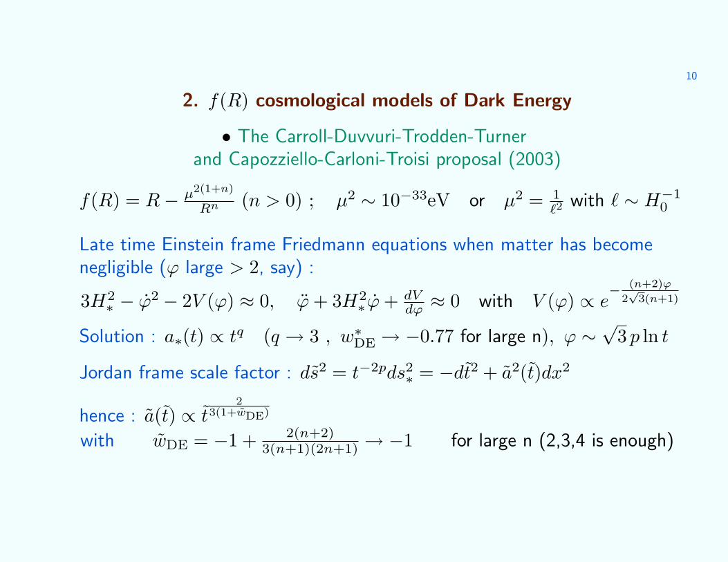
2. f(R) cosmological models of Dark Energy

• The Carroll-Duvvuri-Trodden-Turnerand Capozziello-Carloni-Troisi proposal (2003)

f(R) = R− µ2(1+n)

Rn (n > 0) ; µ2 ∼ 10−33eV or µ2 = 1`2

with ` ∼ H−10

Late time Einstein frame Friedmann equations when matter has becomenegligible (ϕ large > 2, say) :

3H2∗ − ϕ2 − 2V (ϕ) ≈ 0, ϕ + 3H2

∗ϕ + dVdϕ ≈ 0 with V (ϕ) ∝ e

− (n+2)ϕ

2√

3(n+1)

Solution : a∗(t) ∝ tq (q → 3 , w∗DE → −0.77 for large n), ϕ ∼

√3 p ln t

Jordan frame scale factor : ds2 = t−2pds2∗ = −dt2 + a2(t)dx2

hence : a(t) ∝ t2

3(1+wDE)

with wDE = −1 + 2(n+2)3(n+1)(2n+1) → −1 for large n (2,3,4 is enough)

11

• A first flawAmendola, Polarski, Tsujikawa et al., 2003-2007

Friedmann equations when matter dominates over DE (ρ∗ = e−4ϕ/√

3ρ) :

3H2∗ − ϕ2 ≈ κρ∗ , ϕ + 3H2

∗ϕ ≈κρ∗2√

3, ρ∗ + H∗ρ∗ = − ϕ√

3ρ∗

Hence : a(t) ∝ t1/2 instead of t2/3 (for ϕ ≈ 0, V is negligible, not ϕ)

the CDTT model is ruled out

• Conditions for a standard matter era followed by late acceleration

Introduce the dynamical variables : x1 = − f ′

Hf ′ , x2 = − f6Hf ′ , x3 = − R

6H2

Define r(R) = −Rf ′

f and m(R) = Rf ′′

f ′ (Copeland et al. 1997, 2006)

Write the Friedmann equations as x3H = −x1x3

m − 2x3(x3 − 2) etc ;Find the fixed points such that xi = 0 : P = (x1(m), x2(m), x3(m))

12

The“phase space trajectory” m = m(r) can connect a (saddle) matterpoint

PM = (r ≈ −1,m ≈ 0+) with dm/dr|−1 > −1

to a stable fixed point corresponding to

– either exponential acceleration, PS ∈ r = −2, if 0 < m(−2) ≤ 1

– or a ∝ tr, r > 1, PA ∈ m = −(1 + r), if dmdr < −1 and

√3−12 < m < 1

Example :

f(R) = R± µ4+n

Rn with −1 < n < 0

Developments (Capoziello-Tsujikawa, 2007) :

– wDE < −1 for z < zb “crossing of the phantom boundary”

– wDE diverges at z = zc, zb and zc →∞ for n→ −1

13

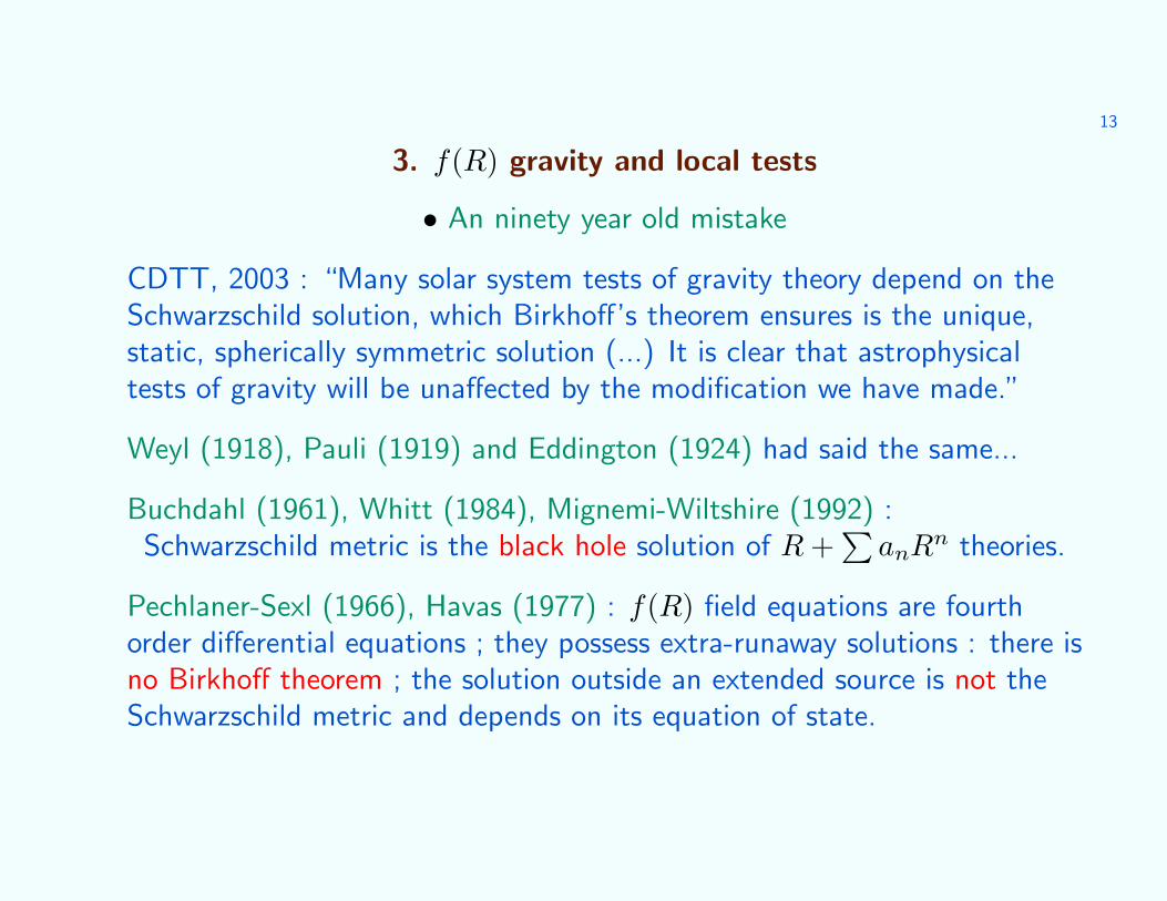
3. f(R) gravity and local tests

• An ninety year old mistake

CDTT, 2003 : “Many solar system tests of gravity theory depend on theSchwarzschild solution, which Birkhoff’s theorem ensures is the unique,static, spherically symmetric solution (...) It is clear that astrophysicaltests of gravity will be unaffected by the modification we have made.”

Weyl (1918), Pauli (1919) and Eddington (1924) had said the same...

Buchdahl (1961), Whitt (1984), Mignemi-Wiltshire (1992) :Schwarzschild metric is the black hole solution of R +

∑anRn theories.

Pechlaner-Sexl (1966), Havas (1977) : f(R) field equations are fourthorder differential equations ; they possess extra-runaway solutions : there isno Birkhoff theorem ; the solution outside an extended source is not theSchwarzschild metric and depends on its equation of state.

14

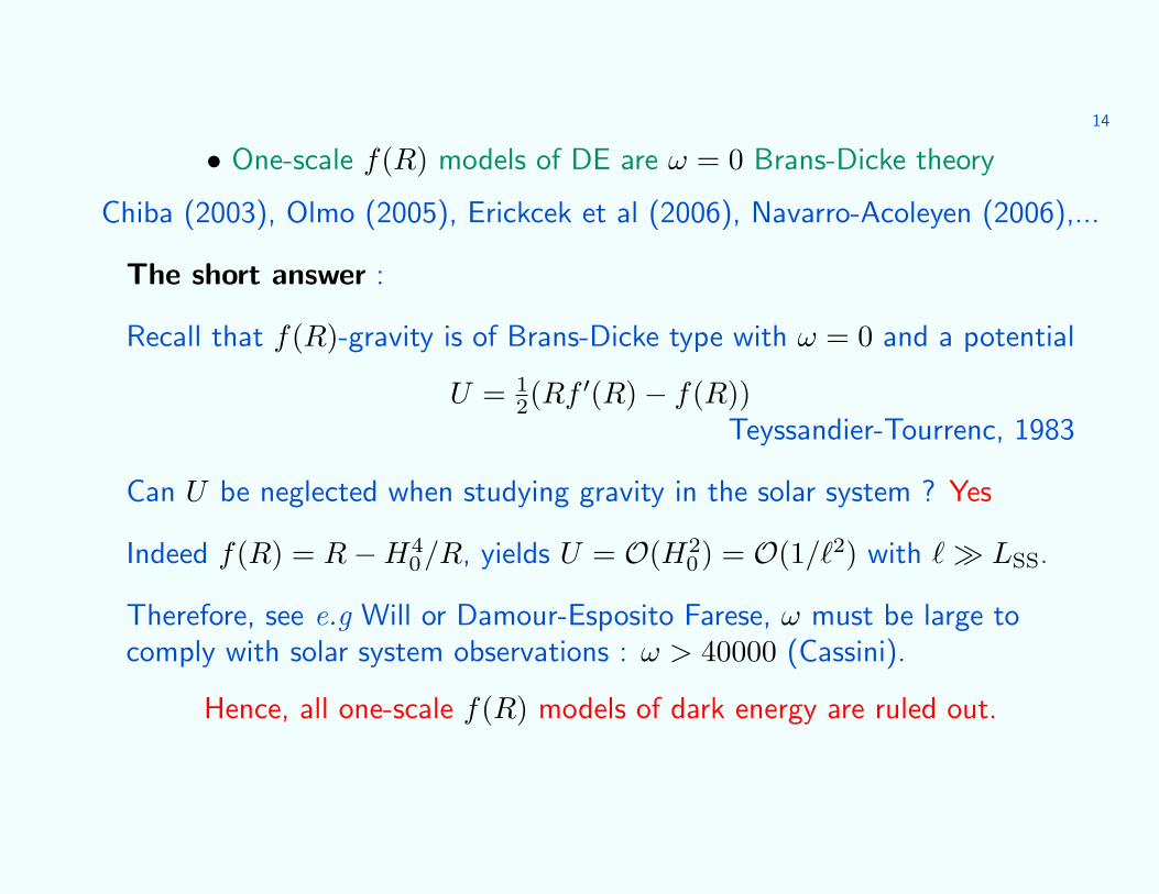
• One-scale f(R) models of DE are ω = 0 Brans-Dicke theory

Chiba (2003), Olmo (2005), Erickcek et al (2006), Navarro-Acoleyen (2006),...

The short answer :

Recall that f(R)-gravity is of Brans-Dicke type with ω = 0 and a potential

U = 12(Rf ′(R)− f(R))

Teyssandier-Tourrenc, 1983

Can U be neglected when studying gravity in the solar system ? Yes

Indeed f(R) = R−H40/R, yields U = O(H2

0) = O(1/`2) with ` LSS.

Therefore, see e.g Will or Damour-Esposito Farese, ω must be large tocomply with solar system observations : ω > 40000 (Cassini).

Hence, all one-scale f(R) models of dark energy are ruled out.

15

The details :

The equations of motion are :

D2∗ϕ−dV

dϕ = 4πG∗√3

T ∗ , G∗ij−2∂iϕ∂jϕ+g∗ij

[(∂∗ϕ)2 + 2V (ϕ)

]= 8πG∗ T ∗

ij

with g∗ij = f ′gij , ρ∗ = ρ/f ′2 , f ′ = e2ϕ/√

3

Linearize : ϕ = ϕc + ϕ1, g∗ij = f ′c(ηij + hij) with Vc = O(κρc) = O(1/`2).

scalaron : 4ϕ1−m2ϕ1 ≈ −4πGeff√3

ρ (4∗ = 4/f ′c , Geff = G∗/f ′c)

m2 = f ′cd2V

dϕ2 |c = O(1/`2) whereas 4 = O(1/L2SS) hence ϕ1 ≈ GeffM√

3r

metric : ds2∗/f ′c ≈ (1− 2GeffM/r)dt2 + (1 + 2GeffM/r)d~x2

ds2 = −(1− 2GM

r

)dt2 +

(1 + 2γGM

r

)d~x2 , G = 4Geff

3 , γ = 1/2

16

A scalar curvature “locked” at its cosmological, small, value :

Equation of motion for the scalar curvature (or scalaron, that is, ϕ) :

3D2f ′ + (Rf ′ − 2f) = κT (not R = κT as in GR !)

Linearize : R = Rc + R1 so that D2R1 −m2R1 = κT3f ′′c

, m2 = (f ′−Rf ′′)|c3f ′′c

Solve with source being, say, a constant density star—or numerically,Multamaki-Vilja, Kanulainen et al, (2007)

and find that, if mr 1, then R ≈ Rc outside and inside the star.

**

On the other hand, if mr 1, find Schwarzschild (hence γ = 1) :

ds2 ≈ −(1− 2GM(1−ε)

r

)dt2 +

(1 + 2GM(1+ε)

r

)d~x2 , ε = e−m(r−r)

2m2r2≈ 0

but... R ≈ −κT Rc inside the star : linear approximation breaks down ?

17

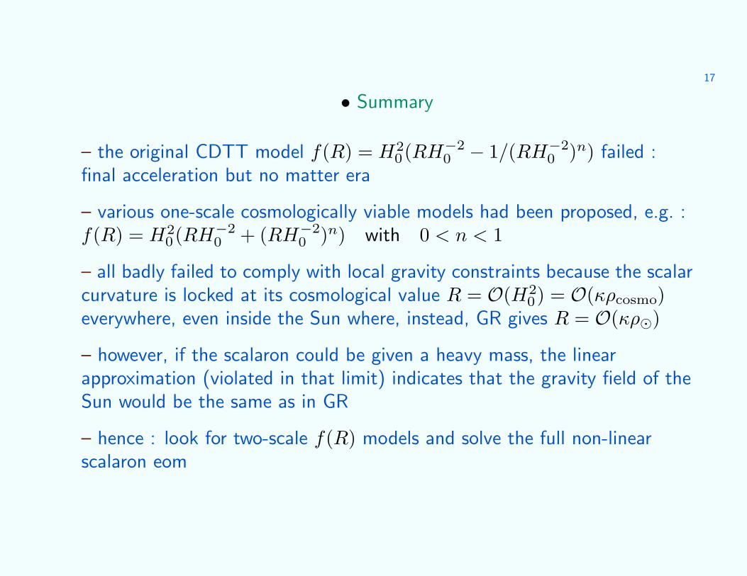
• Summary

– the original CDTT model f(R) = H20(RH−2

0 − 1/(RH−20 )n) failed :

final acceleration but no matter era

– various one-scale cosmologically viable models had been proposed, e.g. :f(R) = H2

0(RH−20 + (RH−2

0 )n) with 0 < n < 1

– all badly failed to comply with local gravity constraints because the scalarcurvature is locked at its cosmological value R = O(H2

0) = O(κρcosmo)everywhere, even inside the Sun where, instead, GR gives R = O(κρ)

– however, if the scalaron could be given a heavy mass, the linearapproximation (violated in that limit) indicates that the gravity field of theSun would be the same as in GR

– hence : look for two-scale f(R) models and solve the full non-linearscalaron eom

18

• Conventional wisdom...e.g. Starobinski, 2007

is based on the linearised scalaron eom on the background dVdϕ |SS ∝ κρ :

4ϕ1 −m2ϕ1 ≈ 0 with m2 = f ′−Rf ′′

3f ′′

If, for R 1/`2, e.g. R ∼ κρ : f ′ → 1 and m2SS ≈ 1

3f ′′|SSis positive and

large ((mL)SS 1) then deviations from Einstein’s GR are small.

CDTT model : m2SS is large and negative (Dolgov-Kawasaki, 2003)

• ...and the “Chameleon” effectKhoury-Weltman (2003)

Navarro-Acoleyen (2006), Capozziello-Tsujikawa (2007)

or : how can the scalar curvature become equal to the local matter density

19

Chameleon details

Once again, look at scalaron eom : D2∗ϕ− dV

dϕ = κ2√

3T∗

In ≈ flat background : 4∗ϕ = dVeffdϕ with dVeff

dϕ = dVdϕ −

κρ∗2√

3

Contrarily to V , Veff may have minima for ϕ = ϕ inside the Sun and forϕ = ϕe outside. One looks for ϕ|e, = ϕ(Re,) such that Re, ≈ κρe,.

Solution outside : ϕ = ϕe + C rr when mer 1 with m2

e = d2Vdϕ2 |e

Solution inside : ϕ ≈ ϕ up to r = r1, then interpolation to ϕ outside.

if r1 ≈ r, then C = 3βClin with β = ϕe−ϕGM/r

≈ ϕeGM/r

One needs β < 10−5 to have γ − 1 < 10−5 (Cassini)

20

• A new family of f(R) models of dark energy

Hu-Sawicki (2007), Starobinski (2007), Odintsov et al (2008), ...

f(R) = R + λRc

[1

(1+R2/R2c)

n − 1], etc

dVdϕ −

κρe

2√

3= 0 gives ϕe = O (ρc/ρe)

2n+1

Now, β ≈ ϕeGM/r

≈ 106ϕe < 10−5 ; hence ϕe < 10−11

For ρe = ρgalaxy = 105ρc then ϕe = O(10−5(2n+1)) and hence the modelsevade Local Gravity Constraints as soon as n > 1/2

In a nutshell : the Chameleon effect conforts conventional wisdom (heavy”local” scalaron mass to evade LGC) : it relies on (1)“locking” ϕ, that is,the scalar curvature, on its Einstein value inside the Sun, and (2) on alocal environment much denser than the asymptotic, cosmological, value.

21

• An uncontrolable scalaron instability ?

The new family of models yield cosmological scale factors which areundistinguishable from Λ-CDM until after the end of the matter era andtend to a de Sitter regime a ∝ eHt.

... However, because the mass of the scalaron is chosen to be high in highmatter density environment (in order to comply with Local gravityConstraints), the cosmological perturbations of the scalaron diverge in theearly matter era unless their amplitude is tuned to a very small value.

Starobinski (2007), Tsujikawa (2007)

22

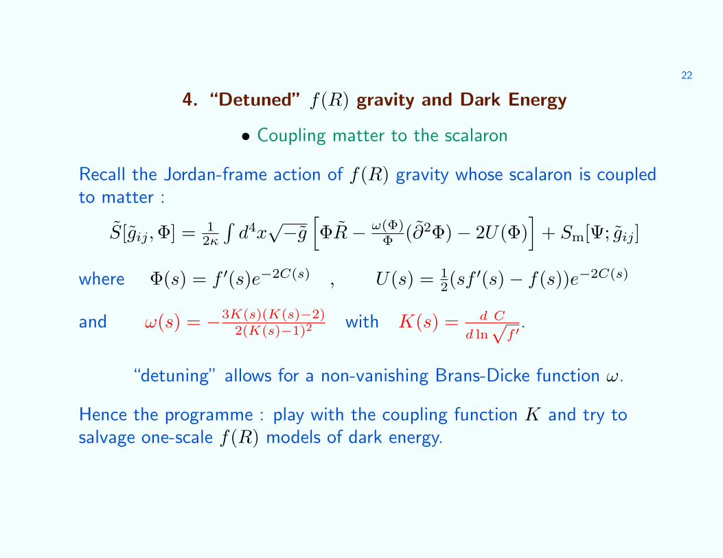
4. “Detuned” f(R) gravity and Dark Energy

• Coupling matter to the scalaron

Recall the Jordan-frame action of f(R) gravity whose scalaron is coupledto matter :

S[gij,Φ] = 12κ

∫d4x√−g

[ΦR− ω(Φ)

Φ (∂2Φ)− 2U(Φ)]

+ Sm[Ψ; gij]

where Φ(s) = f ′(s)e−2C(s) , U(s) = 12(sf

′(s)− f(s))e−2C(s)

and ω(s) = −3K(s)(K(s)−2)2(K(s)−1)2

with K(s) = d C

d ln√

f ′.

“detuning” allows for a non-vanishing Brans-Dicke function ω.

Hence the programme : play with the coupling function K and try tosalvage one-scale f(R) models of dark energy.

23

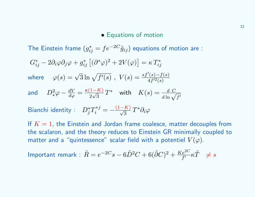
• Equations of motion

The Einstein frame (g∗ij = fe−2C gij) equations of motion are :

G∗ij − 2∂iϕ∂jϕ + g∗ij

[(∂∗ϕ)2 + 2V (ϕ)

]= κ T ∗

ij

where ϕ(s) =√

3 ln√

f ′(s) , V (s) = sf ′(s)−f(s)4f ′2(s)

and D2∗ϕ− dV

dϕ = κ(1−K)

2√

3T ∗ with K(s) = d C

d ln√

f ′

Bianchi identity : D∗jT

∗ji = −(1−K)√

3T ∗∂iϕ

If K = 1, the Einstein and Jordan frame coalesce, matter decouples fromthe scalaron, and the theory reduces to Einstein GR minimally coupled tomatter and a “quintessence” scalar field with a potentiel V (ϕ).

Important remark : R = e−2Cs− 6D2C + 6(∂C)2 + Ke2C

f ′ κT 6= s

24

• Conclusion

– 2003-2007 : five years of trial and errors to conciliate f(R) gravity withcosmology and local gravity constraints

– MANY failed attempts (which reduce to Brans-Dicke with Ω = 0 ; or areunstable)

– Chameleon mechanism and “detuning” : two means to try and save themodels