RIKEN-MP-08

Static interactions and stability of matter in Rindler space

F. Lenz a,c,∗ K. Ohta b,† and K. Yazaki c,d‡

a Institute for Theoretical Physics IIIUniversity of Erlangen-Nurnberg

Staudtstrasse 7, 91058 Erlangen, Germany

b Institute of PhysicsUniversity of Tokyo

Komaba, Tokyo 153, Japan

c Hashimoto Mathematical Physics LaboratoryNishina Center, RIKEN

Wako, Saitama 351-0198, Japan

d Yukawa Institute for Theoretical Physics,Kyoto University

Kyoto 606-8502, Japan

(Dated: December 15, 2010)

AbstractDynamical issues associated with quantum fields in Rindler space are addressed in a study of

the interaction between two sources at rest generated by the exchange of scalar particles, photons

and gravitons. These static interaction energies in Rindler space are shown to be scale invariant,

complex quantities. The imaginary part will be seen to have its quantum mechanical origin in the

presence of an infinity of zero modes in uniformly accelerated frames which in turn are related to

the radiation observed in inertial frames. The impact of a uniform acceleration on the stability of

matter and the properties of particles is discussed and estimates are presented of the instability of

hydrogen atoms when approaching the horizon.

∗ flenz@theorie3.physik.uni-erlangen.de† ohta@nt1.c.u-tokyo.ac.jp‡ yazaki@phys.s.u-tokyo.ac.jp

1

arX

iv:1

012.

3283

v1 [

hep-

th]

15

Dec

201

0

I. INTRODUCTION

The study of quantum fields in Rindler space has played an important role in developingour understanding of quantum fields in non-trivial space-times. The importance of thesestudies derives to a large extent from the existence of a horizon in Rindler space. With itsclose connection to Minkowski space via the known local relation between fields in uniformlyaccelerated and inertial frames, Rindler space provides the simplest possible context toinvestigate kinematics and dynamics of quantum fields close to a horizon.

The kinematics of non-interacting quantum fields in Rindler space [1], [2], [3] and theirrelation to fields in Minkowski space together with the interpretation in terms of quantumfields at finite temperature [4], [5] are well understood. The relation between accelerationand finite temperature remains an important element of the thermodynamics of black holes.Although formally established, the relation between fields in Rindler and Minkowski spaceshas posed some intriguing interpretational problems. Here we mention in particular theissue of compatibility of the radiation generated by a uniformly accelerated charge observedin Minkowski space and the apparent absence of radiation in the coaccelerated frame. Thisproblem was finally resolved by the realization that the counterpart of Minkowski spaceradiation is the emission of zero energy photons in Rindler space [6], [7], [8]. Dynamical issuesof quantum fields have received less attention (cf. [9]). Related to topics to be discussed inthe following are the study of the relation between interacting quantum fields in Minkowskiand Rindler spaces within the path-integral formalism [10], the calculation of level shifts inaccelerated hydrogen atoms [11] and the investigations of the decay of protons [12], [13].

Dynamical issues of quantum fields in Rindler space are in the center of our work. Sub-ject are static forces and their properties relevant for the structure of matter in Rindlerspace. We will study the forces acting between static scalar sources, electric charges andmassive sources generated by exchange of massless scalar particles, photons and gravitonsrespectively. The relevant quantities involved are the corresponding static Rindler spacepropagators. While the time dependent propagators in Rindler and Minkowski spaces aretrivially related to each other by a coordinate transformation with corresponding mixingof the components, this is not the case for the static propagators obtained by integrationover the corresponding time. The different properties of the static propagators reflect thesignificant differences of Rindler and Minkowski space Hamiltonians. Though it was realizedfrom the beginning that the interpretation of Rindler and Minkowski particles (cf. e.g. [1])is different, the differences in the corresponding Hamiltonians have not received sufficientattention. (The identity of the Rindler and Minkowski space Hamiltonians for the frequentlyused special case of a massless field in two dimensional space-time may have obscured theissue.) As shown in [14], the Rindler space Hamiltonian exhibits symmetries which give riseto a highly degenerate spectrum. In particular this degeneracy is also present in the zeroenergy sector. This 2-dimensional sector of zero modes is the image of the photons generatedby the charges uniformly accelerated in Minkowski space. It will be shown to give rise to anunexpected quantum mechanical contribution to the force acting between two charges. Alsothe classical Coulomb-like contribution to the force will be shown to significantly deviatefrom the electrostatic force in Minkowski space. The electrostatic force will be determinedvia Wilson loops and Polyakov loop correlation functions. This method will enable us toseparate the contribution of the quantum mechanical transverse photons from that of theclassical longitudinal field. It will be the method of choice if one attempts to determine thestatic force in simulations of non-abelian gauge theories on a Rindler space lattice.

2

The modifications in the interaction of two charges at rest in Rindler space raise naturallythe question of the stability of atomic systems in Rindler space. We shall investigate thisissue for an ensemble of hydrogen atoms and show within a non-relativistic reduction thatindeed only metastable states exist. We will estimate the probability of ionization as afunction of the distance to the horizon and present arguments concerning the stability ofother forms of matter.

II. PROPAGATORS AND INTERACTIONS OF SCALAR PARTICLES IN RINDLER

SPACE

A. The quantized scalar field in Rindler space

The Rindler space metric [15]

ds2 = e2aξ(dτ 2 − dξ2)− dx2⊥ , (1)

is the (Minkowski) metric seen by a uniformly accelerated observer (acceleration a in x1-direction). Rindler space (τ, ξ) and Minkowski space (t, x1) coordinates are related by

t(τ, ξ) =1

aeaξ sinh aτ , x1(τ, ξ) =

1

aeaξ cosh aτ . (2)

The range of τ, ξ is−∞ ≤ τ , ξ ≤ ∞ , (3)

while the preimage of the Rindler space covers only part of Minkowski space, the right“Rindler wedge”,

R+ =xµ∣∣ |t| ≤ x1

. (4)

The restriction of the preimage of the Rindler space to the right Rindler wedge gives riseto a horizon, the boundary t = ±x1, i.e. ξ = −∞. With this property the Rindler metriccan be identified with other static metrics in the near horizon limit. In particular this is thecase for the Schwarzschild metric which can be approximated in the limit that the distancefrom the horizon is small in comparison to the Schwarzschild radius and if the sphericalSchwarzschild horizon is replaced by a tangential plane.

We start our study of propagators and interactions with a discussion of a scalar field inRindler space (cf. for instance [1], [9]. We will use the notation of [14]). The action of a freemassive scalar field is given by

S =1

2

∫dτ dξ d 2x⊥

∂τφ)2 − (∂ξφ)2 − (m2φ2 + (∂⊥φ)2) e2aξ

. (5)

The wave equation [∂2τ −∆s +m2e2aξ

]φ = 0 , (6)

with the Laplacian∆s = ∂2

ξ + e2aξ∂2⊥ , (7)

is solved by the normal modes (in terms of the McDonald functions)

φω,k⊥(ξ,x⊥) =1

π

√2ω

asinh π

ω

aKiω

a

(1

a

√m2 + k2

⊥eaξ)eik⊥x⊥ , (8)

3

which form a complete, orthonormal set of functions. The normal mode expansion of thescalar field φ reads

φ(τ, ξ,x⊥) =

∫dω√2ω

d2k⊥2π

(a(ω,k⊥)φω,k⊥(ξ,x⊥)e−iωτ + a†(ω,k⊥)φ?ω,k⊥

(ξ,x⊥)eiωτ)

(9)

with the creation and annihilation operators a(†). The stationary states associated with theHamiltonian (π = ∂τφ)

HR =1

2

∫dξd2x⊥

π2 + (∂ξφ)2 + e2aξ

(m2φ2 + (∂⊥φ)2

)=

∫d2k⊥

∫ ∞0

dω ωa†(ω,k⊥)a(ω,k⊥) , (10)

including the lowest energy (ω = 0) state, are degenerate with respect to the value of thetransverse momentum k⊥. This degeneracy has its origin in the appearance of the transversemomentum (in combination with the mass) as a coupling constant of the “inertial potential”e2aξ in the Hamiltonian.

In the Rindler wedge (4), the field operator φ can be represented in terms of plane wavesin Minkowski space or in terms the Rindler space normal modes (9) resulting in the repre-sentation of the Rindler creation and annihilation operators in terms of the correspondingMinkowski space operators. This relation yields the important result for the expectationvalue of the Rindler number operator in the Minkowski ground state |0M〉

〈0M |a†(ω,k⊥)a(ω′,k′⊥)|0M〉 =1

e2π ωa − 1

δ(ω − ω′)δ(k⊥ − k′⊥) (11)

which exhibits a thermal distribution with temperature

T =1

β=

a

2π. (12)

It is important to realize that the infinite degeneracy of the Rindler eigenstates leads, at longwavelengths, effectively to 1-dimensional thermal distributions with weight dω/(e2π ω

a − 1) .

B. The scalar Rindler space propagator

The propagators in Minkowski and Rindler spaces are related to each other by the coordi-nate transformation (2). Written in terms of Rindler and Minkowski coordinates respectively,the propagator of a massless field is given by (cf. [16], [17])

D(τ − τ ′, ξ, ξ′,x⊥ − x′⊥) = i〈0M∣∣T [φ(τ, ξ,x⊥)φ(τ ′, ξ′,x′⊥)

]∣∣0M〉 = D(x− x′)

=1

4iπ2((x− x′)2 − iδ

) =a2e−a(ξ+ξ′)

8iπ2

1

cosh a(τ − τ ′)− cosh η − iδ, (13)

with the notations

D(τ − τ ′, ξ, ξ′,x⊥ − x′⊥) = D(x(τ, ξ,x⊥)− x(τ ′, ξ′,x′⊥)) (14)

4

and

cosh η(ξ, ξ′,x⊥ − x′⊥) = 1 +

(eaξ − eaξ′

)2+ a2

(x⊥ − x′⊥

)2

2ea(ξ+ξ′)= 1 + σ2(ξ, ξ′,x⊥ − x′⊥) .(15)

As we will see, it is η (or equivalently σ) which determines the interaction energies ratherthan the proper distance in Rindler space

d(ξ, ξ′,x⊥ − x′⊥) =

√1

a2

(eaξ − eaξ′

)2+(x⊥ − x′⊥

)2. (16)

The quantity η actually can be viewed as the proper distance in the 4-dimensional AdS space.The appearance of this geometry (of a three-hyperboloid) has been noted [5] in the context ofthe unusual density of states in the photon energy momentum tensor in Rindler space. Thequantity η or equivalently σ exhibits the remarkable invariance under the transformation

ξ, ξ′ → ξ + ξ0, ξ′ + ξ0 , x⊥, x

′⊥ → eaξ0x⊥, e

aξ0x′⊥ . (17)

The coordinate transformation (17) together with a rescaling of the fields φ(τ, ξ,x⊥) →eaξ0φ(τ, ξ,x⊥) leaves, for m = 0, the Hamiltonian (10) invariant and gives rise to the de-generacy of the spectrum. The invariance under scale transformations can be generalized tomassive particles [14].

In Rindler space coordinates the 2-point function (13) satisfies(∂2τ − ∂2

ξ − e2aξ∂2⊥)D(τ, ξ, ξ′,x⊥) = δ(τ)δ(ξ − ξ′)δ(x⊥) . (18)

After a Wick rotation of the Rindler time,

τ → τE = −iτ , (19)

the propagator is periodic in the imaginary time with periodicity β (cf. Eq. (12))

DE(τE, ξ, ξ′,x⊥) =

a2e−a(ξ+ξ′)

8iπ2

1

cos aτE − cosh η − iδ. (20)

In the context of the electromagnetic field we will compute observables in both the realand imaginary Rindler time formalisms. (For discussions of “Euclidean” Rindler spacepropagators, in particular of their topological interpretation cf. [18], [19], [20].)

Without reference to the Minkowski space propagator, Eq. (13) can be derived alterna-tively via the normal mode decomposition (9) in Rindler space. With the help of Eq. (11)the result

D(τ, ξ, ξ′,x⊥) = D(R)(τ, ξ, ξ′,x⊥) + i

∫ ∞0

dΩ

Ω

∫d2k⊥(2π)2

φΩ,k⊥(ξ,x⊥)φΩ,k⊥(ξ′,0⊥)cos Ωτ

e2πΩa − 1

(21)

is obtained where the propagator defined with respect to the Rindler space vacuum is givenby

D(R)(τ, ξ, ξ′,x⊥) = i〈0R∣∣T [φ(τ, ξ,x⊥)φ(0, ξ′,0⊥)

]∣∣0R〉= i

∫ ∞0

dΩ

2Ω

∫d2k⊥(2π)2

φΩ,k⊥(ξ,x⊥)φΩ,k⊥(ξ′,0⊥)e−iΩ|τ | =a2e−a(ξ+ξ′)η

4iπ2 sinh η

1

a2τ 2 − η2 − iδ. (22)

5

(For an interpretation of the difference between the two propagators D −D(R) in terms ofimage charges located in the left Rindler wedge |t| ≤ −x1, cf. [21].) Obviously, the propagatorD(R) depends parametrically on the acceleration a. In order to formulate properly therelation between propagators in Minkowski and Rindler spaces one has to define the Rindlerspace propagator for a fixed value of the acceleration a at finite temperature (given by β)

Da,β(τ, ξ, ξ′,x⊥) = i1

tr e−βHR(a)tre−βHR(a)T

[φ(τ, ξ,x⊥)φ(0, ξ′,0⊥)

]. (23)

In terms of the propagator Da,β, the central result concerning the relation between Rindlerand Minkowski spaces is the identity

i〈0M∣∣T [φ(τ, ξ,x⊥)φ(0, ξ′,0⊥)

]∣∣0M〉 = Da, 2πa

(τ, ξ, ξ′,x⊥) , (24)

i.e., the Rindler space propagator defined with respect to the Minkowski ground state co-incides with the Rindler space finite temperature propagator with the value of the tem-perature determined by the acceleration a (cf. Eq. (12)). This identity makes also manifestthat a change in the acceleration a does not correspond to a change in temperature of theaccelerated system. The acceleration appears not only as temperature in the Boltzmannfactor but also as a parameter in the Hamiltonian (10) of the accelerated system. We willencounter observables which make explicit this twofold role of the acceleration.

The basic quantity in the following investigation of the properties and consequences ofinteractions generated by exchange of scalar particles and photons is the static propagator

D(ω, ξ, ξ′,x⊥) =

∫ ∞−∞

dτeiωτD(τ, ξ, ξ′,x⊥) . (25)

For vanishing mass the k⊥-integration in (21) can be carried out in closed form (cf. [22] and[23])

D(ω, ξ, ξ′,x⊥) =a

4πea(ξ+ξ′) sinh η

(ei

|ω|ηa +

2i sin |ω|ηa

e2π|ω|a − 1

). (26)

Alternatively, this result can be obtained by a contour integration of Eq. (13) in the complexτ plane. The first term is due to the pole infinitesimally close to the real axis τ = η + iδwhile the second, imaginary contribution is the result of the summation of the residues ofthe poles at τn = η+2inπ, n ≥ 1. The result for the static propagator and its decompositioninto the real non-thermal and the imaginary thermal contributions read

D(0, ξ, ξ′,x⊥) = D(R)(0, ξ, ξ′,x⊥) +i

2πβ

η

ea(ξ+ξ′) sinh η

∣∣β= 2π

a

=a

4πea(ξ+ξ′)

1

sinh η

[1 +

iη

π

].

(27)The imaginary part of the static propagator D arises since the propagator (21) is definedwith respect to the Minkowski rather than to the Rindler ground state.

C. The interaction energy of scalar sources

Given the propagator, the interaction energy between two scalar sources is obtained byadding to the action (5) the scalar particle-source vertex

Sint = −∫dv0Hint = κ0

∫d4v√|g(v)| ρ(v)φ(v) , (28)

6

where v stands for either Minkowski (x) or Rindler coordinates (τ, ξ,x⊥). The effectiveaction (the generating functional of connected diagrams) associated with the source is givenby

Wsc = −1

2κ2

0

∫d4v√|g(v)| ρ(v)

∫d4v′

√|g(v′)| ρ(v′)D(v, v′) . (29)

For two point like sources moving along the trajectories vi(si) which are parametrized interms of their proper times si, we find√

|g(v)|ρ(v) =∑i=1,2

∫dsi δ

4(v − vi(si)) . (30)

We assume the sources to be at rest in Rindler space and evaluate Wsc by expressing theproper times si by the coordinate times τi and obtain for sources positioned at ξi,x⊥ i

Wsc = −1

2

∑i,j=1,2

κ(ξi)κ(ξj)

∫dτi

∫dτ ′jD

(τi − τ ′j, ξi, ξj,xi⊥ − xj⊥

). (31)

We have introduced the effective coupling constant

κ(ξ) = eaξκ0 , (32)

which, due to the difference between proper and coordinate times,“runs” with the coordi-nates ξi of the charges. With the sources at rest, Wsc depends only on the differences of thetimes τi. After carrying out the τi integrations, up to a factor T , the size of the interval inthe integration over the sum of the times, Wsc is determined by the static propagator andyields for i 6= j the interaction energy of two scalar sources

Vsc = −κ(ξ1)κ(ξ2)D(ξ1, ξ2,x⊥ 1 − x⊥ 2

)= − aκ2

0

4π sinh η

[1 +

iη

π

], (33)

where η = η(ξ1, ξ2,x1⊥ − x2⊥) (cf. Eq. (15)). For two sources at rest in Minkowski space,this procedure yields the interaction energy −κ2

0/∣∣x1 − x2

∣∣.The interaction energy (33) constitutes an explicit example of the bivalent role of the

acceleration a. The a dependence of the real part of the interaction is exclusively dueto the dependence of the Hamiltonian (10) on the parameter a while the imaginary partdepends in addition on the acceleration via the temperature β = 2π/a (cf. Eq. (27)). Theappearance of a non-trivial imaginary contribution to the “static interaction” generated byexchange of scalar particles and, as we will see also by photons or gravitons, is a novelphenomenon not encountered in the static interactions in Minkowski space. Here we willanalyze this phenomenon. Other properties of the interaction (33) will be discussed later inthe comparison with the “electrostatic” interaction.

As follows from Eq. (18) the static propagator (27) satisfies the Poisson equation fora point-like source in Rindler space. Since the source is real, the imaginary part of thepropagator satisfies the corresponding (homogeneous) Laplace equation. In turn, this impliesthat the imaginary part of propagator or the interaction energy can be represented by a linearsuperposition of zero modes of the Laplace operator (7). From Eq. (21) we read off

Im D(0, ξ, ξ′,x⊥ − x′⊥) =a η

4π2ea(ξ+ξ′) sinh η

=1

4π3a

∫d2k⊥e

ik⊥(x⊥−x′⊥)K0

(k⊥aeaξ)K0

(k⊥aeaξ

′). (34)

7

It is instructive to compare the Rindler space propagator with the finite temperature prop-agator in Minkowski space. As above we decompose the propagator of a non interactingscalar field into thermal and non-thermal contributions

Dβ(x) = i1

tr e−βHMtre−βHMT

[φ(x)φ(x′)

]=

im

4π2√−x2 + iε

K1

(m√−x2 + iε

)+ δDβ(x) , (35)

carry out the Fourier transform of the thermal part

δDβ(ω,x) =

∫ ∞−∞

dt δDβ(x)eiωt =i

2πxθ(ω2 −m2)

sin(√

ω2 −m2x)

eβ|ω| − 1, (36)

and obtain for massless particles

m = 0 , Dβ(0,x− x′) =

∫ ∞−∞

dtDβ(t,x− x′) =1

4π|x− x′|+

i

2πβ. (37)

The Fourier transformed thermal propagators in Rindler (27) and in Minkowski space (37)become identical to order O(a) apart from the factor e−a(ξ+ξ′) and differ from the corre-sponding ground state contribution only by the constant i/2πβ. The convergence to thislimit is not uniform in Rindler space, since it requires a|ξ| , a|ξ′| 1. Due to the twofoldrole of the acceleration a the finite temperature contribution to the propagator in Minkowskispace is only part of the leading order correction to the propagator (cf. Eq. (27)) in Rindlerspace. The structure of the Minkowski space static propagator suggests that the imaginarypart is due to on-shell propagation of zero-energy massless particles. The difference betweenRindler and Minkowski space propagators is due to the different dimensions (0 and 2 respec-tively) of the space of zero modes. Furthermore, while the Minkowski space zero mode isconstant, the zero modes in Rindler space exhibit a non-trivial dependence on all the threecoordinates. Finally for massive particles no zero mode exists in Minkowski space (Eq. (36))while in Rindler space together with the degeneracy in the spectrum also the zero modespersist. In this case the spectral representation in Eq. (34) remains valid provided we replacek2⊥ → k2

⊥ +m2 in the arguments of the McDonald functions.The imaginary part of the propagator determines the particle creation and annihilation

rates. To leading order in the coupling constant κ0, the probability for a change in the initialstate in the time interval [τ0, τ ] is given by (cf. Eqs. ((28)-(32))

Pex(τ, τ0) = 1−∣∣∣〈0M |T e−i ∫ ττ0 dτ ′Hint(τ

′)|0M〉∣∣∣2≈Re

∫ τ

τ0

dτ ′∫ τ

τ0

dτ ′′〈0M∣∣T [Hint(τ

′)Hint(τ′′)]∣∣0M〉

≈ Im

∫ τ

τ0

dτ ′∫ τ

τ0

dτ ′′∑i,j=1,2

κ(ξi)κ(ξj)D(τ ′ − τ ′′, ξi, ξj,x⊥ i − x⊥ j) . (38)

The rate for a change in the initial state within an arbitrarily large time interval T is easilyobtained to be

1

TPex(T, 0)→ Im

∑i,j=1,2

κ(ξi)κ(ξj)D(0, ξi, ξj,x⊥ i − x⊥ j)

=κ2

0a

2π2

(1 +

η(ξ1, ξ2,x⊥ 1 − x⊥ 2)

sinh η(ξ1, ξ2,x⊥ 1 − x⊥ 2)

). (39)

8

The total response (not observable in the accelerated frame) of the field to external sourcesdetermines the imaginary part of the static propagator. Furthermore by defining the reactionrate in terms of the proper time of the external sources (cf. [6], [7], [9], [8]) it is seen that theimaginary part is determined by the total rate for Bremsstrahlung of uniformly acceleratedsources observable in Minkowski space.

These results imply, that under the transformation from the inertial to the acceleratedsystem comoving with the uniformly accelerated charge, the particles generated in Minkowskispace by Bremsstrahlung are mapped into zero energy excitations in Rindler space. In thisway the conflict between particle production in Minkowski space and the conservation ofenergy in Rindler space in the presence of static sources is resolved. The on-shell zeromodes describe the radiation field in Rindler space without any change in the energy inRindler space and may be viewed as a “polarization” cloud of on-shell particles induced byexternal sources or by classical detectors (cf. [24], [25], [26], [27]). Similar remarks apply forthe acceleration induced decay of protons [12], [13]. Essential for this important role of thezero modes is, as indicated above, the peculiar symmetry of the Rindler Hamiltonian whichgives rise to the extensive degeneracy.

III. WILSON AND POLYAKOV LOOPS OF THE MAXWELL FIELD

A. Wilson loops in Minkowski and Rindler space

In this section we consider the Maxwell field coupled to external charges given by theaction

S = −1

4

∫dτdξd2x⊥

√|g|F µνFµν + Sint , Sint =

∫dτdξd2x⊥

√|g|Aµ jµ . (40)

With changing emphasis we will describe various methods for evaluating the interactionenergy of static sources. The computation of Wilson loops [28] and Polyakov loop correlationfunctions [29] constitute the preferred techniques in analytical and numerical studies ofinteraction energies of static sources in gauge theories. In the comparison of these twomethods the emphasis will be on the consequences of the Wick rotation to imaginary timefor the interaction energy which will be seen to be of relevance also for static interactionsin Yang-Mills theories. Evaluation of the Wilson loops in different gauges will enable us toidentify the origin of real and imaginary parts respectively of the electrostatic interaction.

Wilson loops are defined as integrals over the gauge field along a closed curve C in space-time

eiWC = eie∮C dx

µAµ . (41)

The invariance of the Wilson loop under gauge and (general) coordinate transformationsand reparameterization which is explicit in Eq. (41) makes the Wilson loop a particularlyuseful tool for our purpose. Up to self energy contributions, the interaction energy of twooppositely charged sources is given by the expectation value (e.g. in the Minkowski spaceground state) of a rectangular Wilson loop in a time-space plane with side lengths T and R

Σ± = limT→∞

1

TWC[R,T ] , (42)

9

with the ground state expectation value WC[R,T ]

eWC[R,T ] = 〈0M |eiWC[R,T ]|0M〉 . (43)

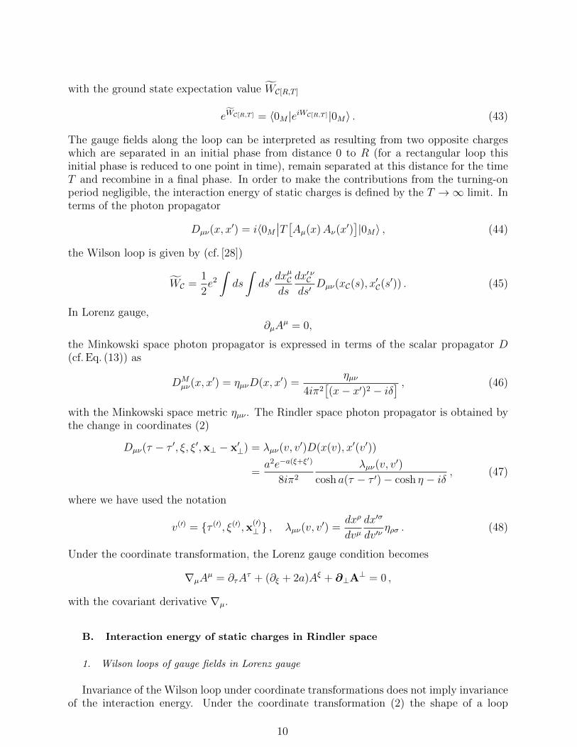
The gauge fields along the loop can be interpreted as resulting from two opposite chargeswhich are separated in an initial phase from distance 0 to R (for a rectangular loop thisinitial phase is reduced to one point in time), remain separated at this distance for the timeT and recombine in a final phase. In order to make the contributions from the turning-onperiod negligible, the interaction energy of static charges is defined by the T →∞ limit. Interms of the photon propagator

Dµν(x, x′) = i〈0M

∣∣T [Aµ(x)Aν(x′)]|0M〉 , (44)

the Wilson loop is given by (cf. [28])

WC =1

2e2

∫ds

∫ds′

dxµCds

dx′ νCds′

Dµν(xC(s), x′C(s′)) . (45)

In Lorenz gauge,∂µA

µ = 0,

the Minkowski space photon propagator is expressed in terms of the scalar propagator D(cf. Eq. (13)) as

DMµν(x, x

′) = ηµνD(x, x′) =ηµν

4iπ2[(x− x′)2 − iδ

] , (46)

with the Minkowski space metric ηµν . The Rindler space photon propagator is obtained bythe change in coordinates (2)

Dµν(τ − τ ′, ξ, ξ′,x⊥ − x′⊥) = λµν(v, v′)D(x(v), x′(v′))

=a2e−a(ξ+ξ′)

8iπ2

λµν(v, v′)

cosh a(τ − τ ′)− cosh η − iδ, (47)

where we have used the notation

v(′) = τ (′), ξ(′),x(′)⊥ , λµν(v, v

′) =dxρ

dvµdx′σ

dv′νηρσ . (48)

Under the coordinate transformation, the Lorenz gauge condition becomes

∇µAµ = ∂τA

τ + (∂ξ + 2a)Aξ + ∂⊥A⊥ = 0 ,

with the covariant derivative ∇µ.

B. Interaction energy of static charges in Rindler space

1. Wilson loops of gauge fields in Lorenz gauge

Invariance of the Wilson loop under coordinate transformations does not imply invarianceof the interaction energy. Under the coordinate transformation (2) the shape of a loop

10

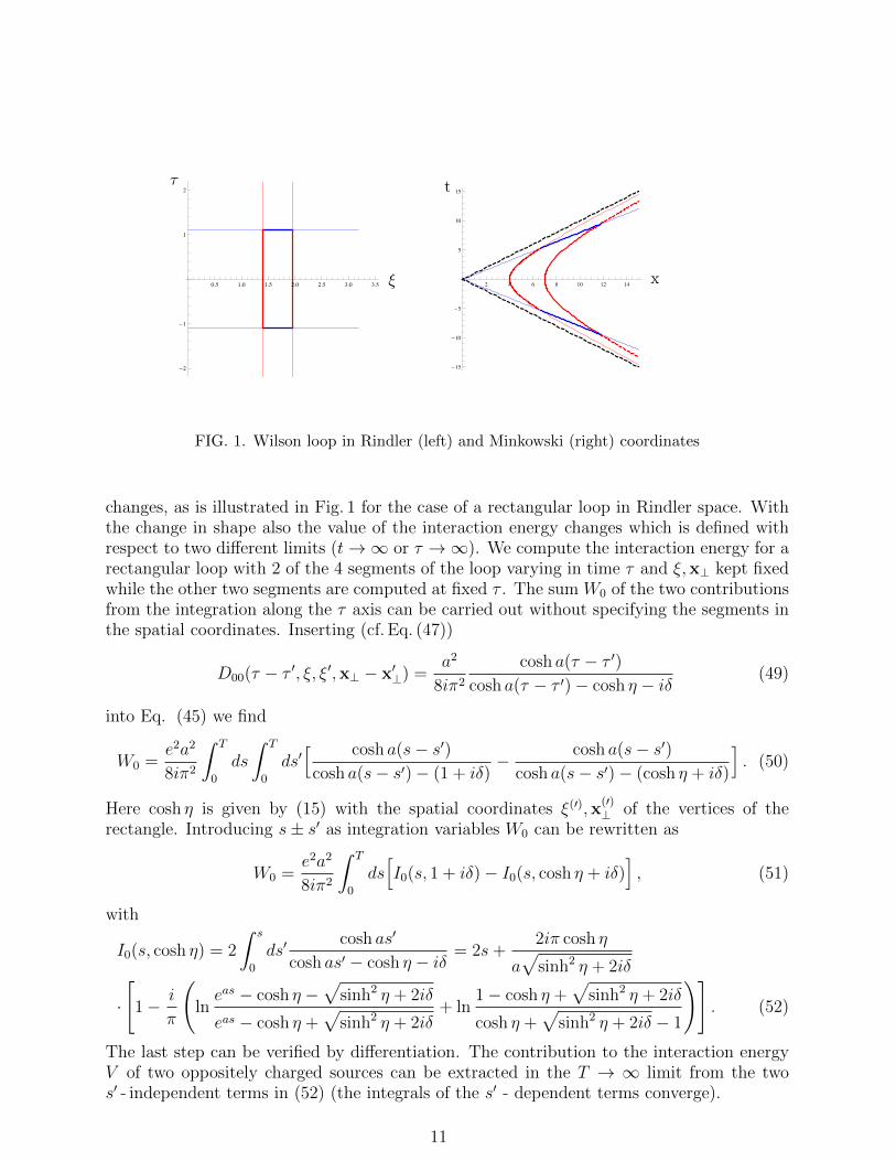
0.5 1.0 1.5 2.0 2.5 3.0 3.5

!2

!1

1

2

!

!

2 4 6 8 10 12 14

!15

!10

!5

5

10

15

x

t

FIG. 1. Wilson loop in Rindler (left) and Minkowski (right) coordinates

changes, as is illustrated in Fig. 1 for the case of a rectangular loop in Rindler space. Withthe change in shape also the value of the interaction energy changes which is defined withrespect to two different limits (t→∞ or τ →∞). We compute the interaction energy for arectangular loop with 2 of the 4 segments of the loop varying in time τ and ξ,x⊥ kept fixedwhile the other two segments are computed at fixed τ . The sum W0 of the two contributionsfrom the integration along the τ axis can be carried out without specifying the segments inthe spatial coordinates. Inserting (cf. Eq. (47))

D00(τ − τ ′, ξ, ξ′,x⊥ − x′⊥) =a2

8iπ2

cosh a(τ − τ ′)cosh a(τ − τ ′)− cosh η − iδ

(49)

into Eq. (45) we find

W0 =e2a2

8iπ2

∫ T

0

ds

∫ T

0

ds′[ cosh a(s− s′)

cosh a(s− s′)− (1 + iδ)− cosh a(s− s′)

cosh a(s− s′)− (cosh η + iδ)

]. (50)

Here cosh η is given by (15) with the spatial coordinates ξ(′),x(′)⊥ of the vertices of the

rectangle. Introducing s± s′ as integration variables W0 can be rewritten as

W0 =e2a2

8iπ2

∫ T

0

ds[I0(s, 1 + iδ)− I0(s, cosh η + iδ)

], (51)

with

I0(s, cosh η) = 2

∫ s

0

ds′cosh as′

cosh as′ − cosh η − iδ= 2s+

2iπ cosh η

a√

sinh2 η + 2iδ

·

[1− i

π

(lneas − cosh η −

√sinh2 η + 2iδ

eas − cosh η +√

sinh2 η + 2iδ+ ln

1− cosh η +√

sinh2 η + 2iδ

cosh η +√

sinh2 η + 2iδ − 1

)]. (52)

The last step can be verified by differentiation. The contribution to the interaction energyV of two oppositely charged sources can be extracted in the T → ∞ limit from the twos′ - independent terms in (52) (the integrals of the s′ - dependent terms converge).

11

For large T , the integration along the spatial segments of the rectangle (the horizontalsegments of the loop in Fig. 1) yields a T -independent term and does therefore not contributeto the interaction energy. The non-diagonal element D01 gives rise to two space-time con-tributions to the Wilson loop which in the large T limit become independent of the spatialcoordinates and cancel each other. Thus we obtain the asymptotic value Σ of the Wilsonloop expressed in terms σ (15)

Σ±(σ) = limT→∞

1

TW0 = − e

2

4πa coth η

[1 +

iη

π

]+ U0 = V (σ) + U0 , (53)

with the interaction energy

V (σ) = − e2

4πa

1 + σ2

√2σ2 + σ4

[1 +

i

πln

√2σ2 + σ4 + σ2

√2σ2 + σ4 − σ2

]. (54)

The integration “constant” U0 arises from the first term in (50) and represents the self-energy of the static charges. Regularizing the divergent integrals by point splitting, U0 isgiven in terms of the proper distance in AdS4 (cf. Eq. (15))

U0 =e2a

8π

( 1√2δσ(ξ)

+1√

2δσ(ξ′)+

2i

π

), δσ2(ξ(′)) =

a2

2

(δξ2 + e−2aξ(′)

δx2⊥). (55)

Before discussing the properties of the “electrostatic” interaction and the comparison withthe static scalar interaction we briefly describe a simple alternative method for calculatingthe interaction energy of two static charges. In analogy with the corresponding calculationfor scalar fields (cf. Eqs. (28)-(32)) the current jµ in Eq. (40) generated by two charges movingalong the trajectories is parametrized as√

|g|jµ(v) =∑i

ei

∫dsi

dvµi (si)

dsiδ4(v − vi(si)) , (56)

resulting in the photon-charge vertex

Sint =∑i

ei

∫dsiAµ(vi(si))

dvµidsi

. (57)

As for the scalar case (Eqs. (28)-(32)), the relevant quantity to be computed is the effectiveaction which, for charges at rest in Rindler space, yields the sum of interaction and selfenergies

Wvc =1

2

∑i=1,2

eiej

∫dsi

∫dsjDµν

(vi(si), vj(sj)

)dvµi (si)

dsi

dvνj (sj)

dsj

=1

2

∑i,j=1,2

eiej

∫dτi

∫dτjD00

(τi − τj, ξi, ξj,xi⊥ − xj⊥

), (58)

where the propagators in different coordinates are obtained from each other by the corre-sponding coordinate transformations (cf. Eq. (47)). Unlike in the scalar case, for exchangeof photons no factor renormalizes the coupling constants when changing from the proper si

12

to coordinate time τ . We define the Fourier transform in time of the 00-component of thepropagator (Eq. (49)) by the limit

D00(ω, ξ, ξ′,x⊥) = limT→∞

∫ T

−TdτeiωτD00(τ, ξ, ξ′,x⊥)

=a2 sinωT

4iπ2ω+

a

4πcoth η

[e−i

ωηa +

2i sin ωηa

1− e−2π ωa

], (59)

and disregarding the (divergent) constant, for opposite charges e = e1 = −e2, the result (54)

− e2D00(0, ξ, ξ′,x⊥) = V (σ) , (60)

is reproduced.

σ2 4 6 8

2.5

2.0

1.5

1.0

0.5

FIG. 2. Real (solid) and imaginary (dashed) parts of the interaction energies 4πVsc/aκ20 (33)

and 4πV/ae2 (54) generated by scalar particle (blue) and photon (red) exchange respectively as a

function of σ (15).

In Fig. 2 are plotted real and imaginary parts of the interaction energy of two staticcharges in comparison with the interaction energy of two scalar sources. The distance whichdetermines both scalar (33) and vector (54) interaction energies is the proper distance of theAdS4 space and not of Rindler space, i.e., the static interaction energies generated by scalarparticle and photon exchange are invariant under the scale transformation (17). At smalldistances where the effect of the inertial force is negligible both interaction energies displaythe familiar linear divergence in the real part and as in Minkowski space, vector and scalarexchange give rise to the same behavior. For small distances the imaginary part is constantand agrees with the constant in the finite temperature propagator (37) in Minkowski space

limσ→0

V (σ) = −e2a

4π

[ 1√2σ

(1 +

3

4σ2)

+i

π

(1 +

2

3σ2)], (61)

limσ→0

Vsc(σ) = −κ20a

4π

[ 1√2σ

(1− 1

4σ2)

+i

π

(1 +

2

3σ2)]. (62)

With increasing distance the inertial forces become important. They weaken both scalarand vector interaction energies and change completely the asymptotic behavior

limσ→∞

V (σ) = −e2a

4π

(1 +

1

2σ4+i

πln 2σ2

), (63)

limσ→∞

Vsc(σ) = −κ20a

4π

1

σ2

(1 +

i

πln 2σ2

). (64)

13

Significant differences in the asymptotics for scalar and vector exchange are obtained. Qual-itative differences are observed for the imaginary part which vanishes asymptotically forscalar exchange and diverges logarithmically with σ for photon exchange. Given the highlyrelativistic motion of the sources in Minkowski space, spin effects are expected to be im-portant. Indeed the comparison of Eqs. (33) and (53) shows that the differences betweenscalar and vector exchange are due to the additional cosh η factor in (53) arising from thetransformation of the propagator from Minkowski to Rindler space. In this context we alsonote the stronger asymptotic suppression of the “electrostatic” force in comparison to theforce generated by scalar exchange. From the point of view of a Minkowski space observer(cf. Eq. (58)), cancellation between magnetic and electric forces generated by the spatialcomponents of the current and by the charges respectively is to be expected.

Of particular interest is the behavior of the interaction energy if one of the sourcesapproaches the horizon while the position of the other source is kept fixed. For

ξh → −∞, σ2 → 1

2e−a(ξh+ξ)

(e2aξ + a2(x⊥ − x′⊥)2

)→∞ , (65)

the interaction energies are given by

limξh→−∞

V (σ) = −e2a

4π

(1− ia(ξh + ξ)

π

), (66)

limξh→−∞

Vsc(σ) = −κ20a

2πea(ξh+ξ) 1

e2aξ + a2(x⊥ − x′⊥)2

(1− ia(ξh + ξ)

π

). (67)

In both cases the interaction is dominated by the imaginary radiative contribution andno bound states are expected in this regime. We also find in analogy with the “no hair”theorem [30], [31], [32] for Schwarzschild black holes that a scalar source close to the horizoncannot be observed asymptotically while vector sources are visible. Formally the differencearises from the running of the scalar coupling (32) to zero when approaching the horizonwhile the electromagnetic coupling remains constant. In detail the results for Rindler andSchwarzschild metrics are different. A significant improvement can be obtained by modifyingthe Rindler metric

ds2 = e2aξ(dτ 2 − dξ2)− dx2⊥ → e2aξ(dτ 2 − dξ2)− 1

4a2dΩ2 . (68)

The dynamics in this space is very close to the dynamics in Rindler space unless the differencebetween the S2 and R2 matters. This is the case when deriving the “no hair” theorem whereonly the l = 0 waves matter [33].

2. Wilson loops of gauge fields in Weyl gauge

In the (covariant) Lorenz gauge only the 00-component of the propagator contributes(cf. Eqs. (54) and (60)) which simplifies significantly the evaluation of the electrostatic inter-action energy and by the same token hides the difference in origin of its real and imaginaryparts. Separation of constrained and dynamical variables becomes manifest in Weyl gauge

A0 = 0 .

14

In this gauge one works with two unconstrained dynamical fields describing the photons anda longitudinal field constraint by the Gauß law. The gauge field is decomposed accordingly

Ai = ∂iχ+ Ai , (69)

into the longitudinal component given by the scalar field χ and the transverse field satisfying

P ijA

j = Ai , with P ij = δij + ∂i

1

∆∂j, (70)

and the Laplacian∆ = −∂i∂i = e−2aξ

(∂2ξ − 2a∂ξ

)+ ∂2

⊥ . (71)

Longitudinal and transverse fields are not coupled to each other. Their actions are given by

S`[χ] = −1

2

∫d4x∂0∂iχ∂0∂

iχ , (72)

and

Str[A] = −1

2

∫d4x∂0Ai∂0A

i − 1

4

∫d4x√|g| gikgjl(∂iAj − ∂jAi)(∂kAl − ∂lAk) . (73)

The Wilson loop expectation value factorizes into transverse and longitudinal contributionsand the corresponding interaction energies (42) are additive. In Weyl gauge, the longitudinalcontribution to the Wilson loop for a rectangle with one pair of its sides being parallel tothe τ axis (τ0 = 0 ≤ τ ≤ τ1 = T ) is given by∮Cdxi∂iχ(τ, ξ,x⊥) =

∫ s1

s0

dsdxi

ds

(∂iχ(0, ξ(s),x⊥(s))−∂iχ(T, ξ(s),x⊥(s))

)=

∫d4x ρ(x)χ(x),

withρ(x) =

∑i,j=0,1

(−1)i+j+1δ(τ − τi)δ(ξ − ξ(sj))δ(x⊥ − x⊥(sj)) .

In terms of the Green’s function associated with the differential operators ∂2τ and the Lapla-

cian (71)

∂2τ

1

2|τ | = δ(τ) , ∆G(ξ,x⊥, ξ

′,x′⊥) = δ(ξ − ξ′)δ(x⊥ − x′⊥) , (74)

we find the following longitudinal contribution to the Wilson loop

W` = −Te2[G(ξ1,x⊥ 1, ξ0,x⊥ 0)− 1

2

∑i=0,1

G(ξi,x⊥ i, ξi,x⊥ i)]. (75)

The Green’s function G has been calculated in [14]. It coincides with the real part of thestatic Lorenz gauge propagator (cf. Eq. (59))

G(ξ,x⊥, ξ′,x′⊥) = Re D00(0, ξ, ξ′,x⊥ − x′⊥) , (76)

and therefore up to irrelevant additive constants (cf. Eq. (54))

V (σ) = −e2G(ξ1,x⊥ 1, ξ0,x⊥ 0) . (77)

15

The transverse gauge field operators required for calculating the transverse contributionto the Wilson loop have been constructed in [14] with the ξ component given by

A1(τ, ξ,x⊥) = e2aξ

∫dω√2ω

d2k⊥2π

k⊥ω

[a1(ω,k⊥)e−iωτ+ik⊥x⊥ + h.c.

]φω,k⊥(ξ,x⊥) . (78)

In order to avoid technical complications we assume the Wilson loop to be located in theτ -ξ plane. Applying the general expression (45) we obtain

Wtr(T, ξ1, ξ2,0⊥) = e2

∫ ξ2

ξ1

dξ

∫ ξ2

ξ1

dξ′DW11 (0, ξ, ξ′,0⊥)−DW

11 (T, ξ, ξ′,0⊥), (79)

with the 11 component of the Weyl gauge propagator

DW11 (τ, ξ, ξ′,x⊥) = i〈0M

∣∣T [A1(τ, ξ,x⊥)A1(0, ξ′,0⊥)]∣∣0M〉 = −ie2a(ξ+ξ′)

∫ ∞0

dω

π2asinh

πω

a

·∫

d2k⊥(2π)2

k⊥2

ω2(e−iω|τ | +

2 cosωτ

e2πωa − 1

)Kiωa

(k⊥aeaξ)Kiω

a

(k⊥aeaξ

′)eik⊥x⊥ . (80)

As above, the interaction energy is determined by the linearly divergent contribution to theWilson loop in the large time limit aT 1 and is generated by the thermal contribution inEq. (80). We obtain for the transverse contribution to the Wilson loop

Wtr(T, ξ1, ξ2,0⊥) = −iT e2a

4π2

(η coth η − 1

), (81)

which coincides with the imaginary part of V (σ) (53) for η = a(ξ1 − ξ2).With the unambiguous separation of constraint and dynamical degrees of freedom in Weyl

gauge, our result underlines the dynamical origin of the imaginary part of the Wilson loopin the large T limit as opposed to the electrostatic origin of the real part. We essentially canapply now the arguments of Sect. II C concerning the imaginary part of the scalar propaga-tor. The photons generated by an accelerated charge in Minkowski space are mapped intozero energy (transverse) photons in Rindler space. Though of zero energy, these transversephotons carry momentum and contribute therefore in a non-trivial way to the interactionenergy. They propagate on the mass shell and their contribution to the interaction energy istherefore purely imaginary. Our derivation of the interaction energy of two static sources inWeyl gauge emphasizes the classical origin of the real part and the quantum mechanical ori-gin of the imaginary part. Thereby it also confirms the relation of the zero modes in Rindlerspace generating the imaginary part with the Bremsstrahlung photons of the acceleratedcharge in Minkowski space.

C. Polyakov loop correlator

In numerical studies of gauge theories at finite temperature on the lattice an importantquantity for characterizing the interaction energy of static charges is the correlation func-tion of Polyakov loops [29]. These studies are carried out on a Euclidean lattice and haveconfirmed the existence of a transition in Yang-Mills theories from the confining to the de-confined phase. It would be of great interest to extend these studies to Rindler space and tofollow the fate of the confined phase when approaching the horizon. In this paragraph we

16

will calculate the Polyakov loop correlator in Rindler space with imaginary (Rindler) time(cf. Eq. (19)) which due to the acceleration is a periodic coordinate. Up to a multiplicationwith i, the “Euclidean” propagators are obtained from the real time propagators ((13) and(47)) by this change of the time coordinate. In particular the relevant component of thegauge field propagator (49) is given by

DE00(τE − τ ′E, ξ, ξ′,x⊥ − x′⊥) =

a2

8π2

cos a(τE − τ ′E)

cos a(τE − τ ′E)− cosh η − iδ. (82)

The periodicity in imaginary time expresses the similarity of acceleration and finite tem-perature. Unlike the temperature, the acceleration a also appears together with the spatialcoordinates. The Polyakov loop is defined by

P (e, ξ,x⊥) = expie

∮dτEA

E0 (τE, ξ,x⊥)

, (83)

and the Polyakov loop correlator associated with two static charges e1,2 located at ξ1,2,x⊥ 1,2

is given byCP (ξ1, ξ2,x⊥ 1,x⊥ ,2

)= 〈0M |P (e1, ξ1,x⊥ 1)P (e2, ξ2,x⊥ 2)|0M〉 . (84)

Written as a path integral, this correlation function is easily evaluated with the result

CP (ξ1, ξ2,x⊥ 1,x⊥ 2

)= e−

2πa

(f11+f22+2f12) , (85)

where the self and interaction energy contributions to the “free energy” fij are given by(cf. Eq. (15))

fij =aeiej32π3

∫ 2π

0

ds

∫ 2π

0

ds′cos(s− s′)

cosh η(ξi, ξj,x⊥ i − x⊥ j)− cos(s− s′)

=aeiej8π

(coth η(ξi, ξj,x⊥ i − x⊥ j)− 1

). (86)

Regularization by point splitting (cf. Eq. (55)) yields the self-energies

fii =e2i

8π

1√δξ2 + e−2aξiδx2

⊥. (87)

The interaction energy of the two charges

VP(ξ1, ξ2,x⊥ 1,x⊥ 2

)=ae1e2

4π

(coth η

(ξ1, ξ2,x⊥ 1 − x⊥ 2

)− 1), (88)

agrees with the real part of the interaction energy obtained in the calculation of the Wilsonloop in Lorenz gauge (54) and with the contribution from the longitudinal degrees of free-dom (77). In agreement with the results of [34] concerning the equivalence of propagatorsdefined in static space-time with either real or imaginary times, the Rindler space propa-gator (cf. Eq. (49)) can be reconstructed given the imaginary time propagator (cf. Eq. (82)).However, unlike in Minkowski space, this reconstruction may not work separately for singleFourier components such as the static component of the propagators. Apparently, the dif-ference between imaginary and real time static propagators of the Maxwell field is due tothe non-trivial (imaginary) contributions to the propagator from zero energy photons. Forthe case of Yang-Mills theories it remains to be seen how this missing information could begained e.g. by studies of appropriate correlation functions.

17

D. Static gravitational interaction in Rindler space

To complete our discussion of static forces in Rindler space we sketch the calculation ofthe gravitational interaction of two point masses M1,2 at rest in Rindler space. We apply thesame method as above and start with the graviton propagator in Minkowski space which inharmonic gauge is, in terms of the scalar propagator (13), given by

Dµν,ρσ = χµν,ρσD(x, x′) , χµν,ρσ =1

2

[ηµρηνσ + ηµσηνρ − ηµνηρσ

], (89)

and ηµν denotes the Minkowski space metric. With the relevant Rindler space tensor com-ponent of χ,

χ′00,00 =1

2e2a(ξ+ξ′) cosh 2a(τ − τ ′) , (90)

the corresponding element of the propagator in Rindler space ordered according to theasymptotics in Rindler time τ reads

D(R)00,00(τ, ξ, ξ′,x⊥) =

a2

4iπ2(cosh aτ + cosh η) ea(ξ+ξ′) + (2 cosh2 η − 1) e2a(ξ+ξ′) D(τ, ξ, ξ′,x⊥) .

(91)As for scalar (31) and vector exchange (58) we introduce also for graviton exchange theeffective action

Wte = −G∑i=1,2

MiMj

∫dsi

∫dsjDµν,ρσ

(vi(si), vj(sj)

)dvµi (si)

dsi

dvνi (si)

dsi

dvρj (sj)

dsj

dvσj (sj)

dsj, (92)

which for the particles at rest in Rindler space represents their interaction and self-energies.As above (cf. Eq. (59)), for calculating the static interaction energy, we define the divergent τintegrals by integrating over a large but finite interval [−T/2, T/2] and obtain from Eq. (92),after performing for the convergent terms the limit T →∞, the following expression for thestatic gravitational interaction energy

Vgr(ξ1, ξ2,x⊥ − x′⊥) = −G∫dξd2x⊥dξ

′d2x′⊥T001 (ξ,x⊥)T 00

2 (ξ′,x′⊥)D(R)00,00(0, ξ, ξ′,x⊥ − x′⊥)

= −GM1M2

a2

2iπ2

(1

asinh

aT

2+T

2cosh η

)+

a

4π

2 cosh2 η − 1

sinh η

[1 +

iη

π

], (93)

where η = η(ξ1, ξ2,x⊥ 1−x⊥ 2) (cf. Eq. (15)) and we have used the energy momentum tensordensity of 2 particles at rest in Rindler space

T µνi (ξ,x⊥) = Mie−aξδ(ξ − ξi)δ(x⊥ − x⊥ i)δµ 0δν 0 . (94)

We note that the interaction energies for the three cases considered (Eqs. (33), (53), (93))depend only on the quantity η (15) or equivalently σ and are therefore invariant underthe scale transformation (17). For scalar particle and graviton exchange the explicit ξ, ξ′

dependent factors of propagators and vertices (cf. (27), (28) and (92)) cancel each otherwhile both photon propagator (49) and vertex (57) depend only on η

The terms divergent in the T → ∞ limit are imaginary. They therefore satisfy thewave equation and are to be interpreted as the image of the gravitational radiation ofthe accelerated particles in Minkowski space. Both the imaginary contribution from the

18

radiation and the real “static” gravitational interaction diverge with η. If evaluated inMinkowski coordinates, the source of these divergences of Wte is not the propagator but theenergy momentum tensor of uniformly accelerated particles

T µνi = Mia

x1eaξ0δ(x⊥ − x⊥ i)δ

(x1 −

√t2 + a−2e2aξ0

)·[x1 2δµ 0δν 0 + x1t(δµ 0δν 1 + δµ 1δν 0) + t2δµ 1δν 1

]. (95)

The energy density as well as the density of the momentum in 1 direction and also theflux of the 1-component of the momentum in the 1 direction increase for sufficiently largepositive or negative times like |t|. Thus the exponential increase of the graviton propagatorwith τ and with η reflects the increase of the energy and momentum density in Minkowskispace. Ultimately this increase invalidates the linearization of the Einstein equations andthe backreaction on the gravitational field by the increasing energy-momentum tensor inMinkowski space or equivalently by the increasing propagator in Rindler space has to betaken into account.

IV. HYDROGEN-LIKE SYSTEMS AND THE STABILITY OF MATTER IN

RINDLER SPACE

A. Non-relativistic limit of accelerated atoms

As an application of the formal development we will address in this section the issue ofstability of matter under uniform acceleration. The radical change of the dispersion relationbetween energy and momentum of elementary particles makes it very unlikely that matteras observed in Minkowski space will be formed in an accelerated frame. We will address thisissue in a study of the effect of acceleration on hydrogen-like atoms consisting of an infinitelyheavy, pointlike nucleus of charge Z and a single electron. We will present evidence thatthe atomic structure is destroyed by uniform acceleration.

The acceleration a will be chosen to be small in comparison to the electron mass me inorder to keep the electron motion in the rest frame of the nucleus non-relativistic. Further-more, to simplify the calculation we treat the electron as a scalar particle. Keeping only thecoupling between electron and nucleus via A0, the approximate Lagrangian is

L =√|g| (∂µφ∂µφ† −m2φφ†)− ie2

(D00(0, ξ + ξZ , ξZ ,x⊥) + UZ

0 (ξ + ξZ , ξZ ,x⊥))

·[φ†(ξ,x⊥) φ(ξ,x⊥)− φ†(ξ,x⊥) φ(ξ,x⊥)

], (96)

with the coordinates ξZ ,x⊥Z = 0 and ξ+ξZ ,x⊥ denoting the position of the nucleus andthe electron respectively and with D00 given in Eqs. (54) and (60). Besides the interactionenergy, the Lagrangian also contains the lowest order self energy (cf. Eq. (55))

UZ0 (ξ + ξZ , ξZ ,x⊥) =

e2a

8π

( 1√2δσ(ξ + ξZ)

+Z2

√2δσ(ξZ)

+i(1 + Z2)

π

). (97)

With the Ansatz

φ(τ, ξ,x⊥) = e−iωτϕ(ξ,x⊥) ,

19

the stationary wave equation reads[− ω2 − ∂2

ξ + (−∂2⊥ +m2) e2a(ξZ+ξ) + 2ω Ze2D00(0, ξ + ξZ , ξZ ,x⊥)

+ UZ0 (ξ + ξZ , ξZ ,x⊥)

]ϕ(ξ,x⊥) = 0 . (98)

In the non-relativistic approximation the energy is dominated by the mass term

ω2 = (m+ E)2e2aξZ ≈ (m2 + 2mE)e2aξZ , (99)

and the Hamiltonian associated with the wave equation (98) is given by (cf. Eq. (54))

H = − 1

2m

(e−2aξZ∂2

ξ + e2aξ∂2⊥)

+ e−aξZ(V (σ) + UZ

0

)+m

2

(e2aξ − 1

), (100)

with E denoting an eigenvalue of H. In comparison to the Hamiltonian in Minkowski spaceboth potential and kinetic energies are significantly modified. Only by the requirement ofweak acceleration, i.e. if a is mall in atomic units,

aρB 1 with the Bohr radius ρB =1

mZα, (101)

the connection of H to the Minkowski space Hamiltonian becomes transparent. In general,the macroscopic coordinate of the nucleus ξZ is large on this scale. In this weak accelerationlimit, we replace V (σ) by the leading term in the expansion (61), rescale the variable ξ andthe regulator δξ (cf. Eq. (97))

z = ξeaξZ , δz = δξeaξZ , (102)

and introduce the local acceleration (cf. [15])

aZ = ae−aξZ . (103)

The resulting Hamiltonian reads

H = H0 +W = − 1

2m∆− Zα√

z2 + x2⊥

+maZz +W, (104)

with (cf. Eq. (97))

W = e−aξZ(i ImV (σ) +UZ

0

)=

(Z2 + 1)e2

8π√δz2 + δx2

⊥+iaZe

2

8π2

((Z−1)2− 2Z

3a2Z(z2 +x2

⊥)). (105)

In the weak acceleration limit, the real part of the sum of the electrostatic self energies ofthe electron and the nucleus is a complex constant independent of ξ and can be dropped.

B. The imaginary part of the Coulomb interaction

The imaginary part of the Hamiltonian (104) reflects the presence of on-shell propagatingzero energy photons. The leading term is the self energy of the total charge Z − 1. Itincreases linearly with the local acceleration aZ and expresses the instability of the bare

20

source towards decay into source and zero energy photons. Thus a static charge in Rindlerspace is accompanied by on-shell zero energy photons. This “cloud” of photons is nothing elsethan the image in Rindler space of the Bremsstrahlung photons generated by the acceleratedcharge in Minkowski space.

In a system of two oppositely charged sources (Z = 1) the imaginary part of self energyand interaction energy contributions cancel each other for small distances (cf. Eq. (105)). Inthis limit where the opposite charges neutralize each other, no Bremsstrahlung is generatedin Minkowski space and no zero energy photons in Rindler space. Beyond this limit anddue to the peculiar energy-momentum dispersion relation, a new phenomenon appears. Forvalues of the acceleration of the order of the inverse distance of the two charges, momentumis transferred by the exchange of zero energy photons. As shown in Fig. 2, the correspondingimaginary part of the interaction energy increases logarithmically with the distance σ of thetwo charges giving rise to a long range (imaginary) force between the static charges. Withregard to conceptual issues concerning signatures of the Unruh effect, a detailed study ofthe consequences of this force for the dynamics of electromagnetically bound systems, e.g.,the hydrogen atom, would be of interest. Simple answers can be obtained only in the limitof small acceleration (Eq. (101)). In this limit perturbation theory applied to ImW yieldsthe width of the hydrogen states induced by the acceleration

Γn` =e2

6π2a3Z〈n`| r2 |n`〉 =

e2

12π2a3Zρ

2B

[5n2 + 1− 3`(`+ 1)

].

The inverse of Γ is the time it takes a bare hydrogen atom to get dressed by zero-energyphotons. For this dressing to occur on the atomic time scale, the acceleration aZ has to beof the order of mα and therefore larger by a factor of 1/α2 than typical atomic accelerations.With “macroscopic” accelerations such as the acceleration at the horizon of a black hole,the time it takes to build up the photon cloud is of the order of the age of the universe.

Due to the dependence of ImW on the electron coordinate, initial and final hydrogenstates are not necessarily identical but it appears that energy conservation forbids such atransition. On the other hand, considering the corresponding process in Minkowski space,nothing forbids for instance emission of a Bremsstrahlung photon by an infinitely heavyproton followed by absorption of the (on-shell) photon by the electron and thereby producingan excited state of the hydrogen atom. In Rindler space the on-shell photon is mapped intoa zero mode and therefore the excitation of the atom occurs without energy transfer. Thusground and excited states must be degenerate which in turn suggests that the initial statemust be an ionized state. In the following more detailed calculations we will show that thisindeed is the case.

C. Decay of uniformly accelerated hydrogen-like atoms

In this section we are discussing the effect of the inertial force in hydrogen like atomswhich are at rest in Rindler space. In particular we will discuss the instability of theatomic states due to ionization by the inertial force described by the term linear in z ofthe Hamiltonian (104). For the following discussion the contribution W to the Hamiltonian(104) is irrelevant and will be neglected. The Hamiltonian H0 is the standard non-relativisticHamiltonian of hydrogen-like systems complemented by the dipole term maZz which is thesmall z limit of the inertial force m2e2aξ in the wave-equation (6). As required by the

21

equivalence principle, to leading order in the acceleration a, this additional term appears asan external homogeneous gravitational field.

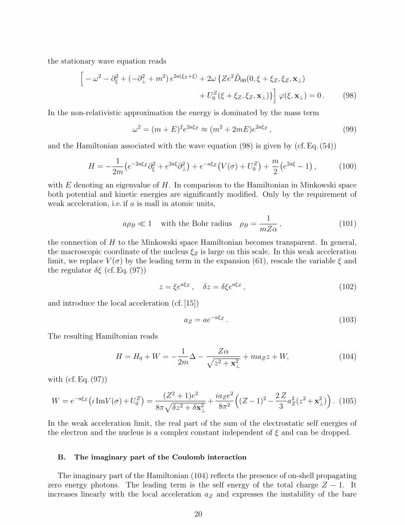
Although of different dynamical origin, the Hamiltonian H0 coincides, after reinterpre-tation of the constants, with that of a hydrogen-like system in the presence of an external,constant electric field. For the analysis of the spectrum we employed the techniques devel-oped for the description of the Stark effect [35], [36], and carried out the computation of theshift in the spectrum and of the lifetime of the ground state by using parabolic coordinates.The nature of the spectrum is determined by the interplay between the inertial force and

-10 -5 5 10

-25

-20

-15

-10

-5

5

FIG. 3. Coulomb potential (blue) and sum of Coulomb and inertial potential (red) in eV along an

axis through the origin tilted with respect to the z-axis by 60 with aρB ≈ 10−7 with the distance

to the origin given in units of the Bohr radius.

the electrostatic force (cf. Eq. (54)) as is demonstrated in Fig. 3. The relative strength ofinertial and electrostatic interactions is given by the parameter

γ =aZ

mZ3α3, (106)

which is the ratio between the local acceleration aZ and the radial acceleration of the electronat the Bohr radius.

When turning on acceleration the first signatures of the presence of inertial forces arechanges in the spectrum. The ground state energy of the hydrogen atom is modified in secondorder perturbation theory (quadratic Stark effect). For γ = 8 ·10−3, i.e. aZ ≈ 7 ·10−20 m s−2,the shift ∆E of the ground state energy E0 is given by

∆E

E0

=9

2γ2 = 0.00029 . (107)

Since the leading term vanishes in lowest order perturbation theory, corrections to the Hamil-tonian H0 (104) proportional to a2

Z have to be considered. The dominant contribution comesfrom the expansion of the inertial force in Eq. (100), ∆2H = ma2

Zz2. In comparison to (107),

the resulting shift of the ground state energy is suppressed by two powers of α

∆2E

∆E= −4

9α2 . (108)

Corrections to the Coulomb interaction (cf. Eqs. (100), (61)) are suppressed by still higherpowers of α.

22

With increasing acceleration we also have to account for the decay of the atom inducedby the inertial force. As Fig. 3 shows, strictly speaking no stable hydrogen bound stateexists whatever the non vanishing value of the acceleration may be, thereby confirming theabove conjecture that existence of the imaginary part together with energy conservation inRindler space is not compatible with the existence of atomic bound states. If on the otherhand we assume that the acceleration has not been present for infinite time i.e. the atomhas not been close to a black hole infinitely long, the lifetime of the atom is a useful quantityto characterize the effect of the acceleration on the stability of matter. In such a case, theatom decays by tunneling of the electron through the potential barrier. With decreasing γthe potential energy approaches the Coulomb potential and the lifetime of the metastablestate tends to infinity. Above a critical value γ = γc where the two turning points coalesce,a meaningful definition of a metastable state becomes impossible. In this regime the inertialforce is dominant and no bound states are formed.

Within the formulation in terms of parabolic coordinates the critical value can be com-puted with the results

γc = 2(3 +√

7)/(2 +√

7)3 = 0.11 , (109)

and the lifetime of the ground state of hydrogen-like systems can be estimated by calculatingthe tunneling probability in the WKB approximation. The resulting expression for the widthreads

Γ = |E0|8

γe−

23γ . (110)

The decay rate of the hydrogen atom is determined by the tunneling probability of theelectron ∼ γ−1 exp−2/3γ and the frequency ∼ |E0| with which the electron reaches theclassically forbidden region. With the above choice of 8·10−3 for the parameter γ the lifetimeof the hydrogen atom is of the order of the age of the universe, while, when increasing theacceleration by a factor of 14 to reach the critical value γc, the width is about 2% of theground state energy and no metastable state is formed.

D. Instability of matter

The decrease of the lifetime of the hydrogen atom is a consequence of the dependenceof the acceleration on the position of the nucleus and is another signature of the spatialvariation of the Tolman temperature appearing for instance in the energy momentum tensorof photons in Rindler space [37], [5]. As a consequence, in an accelerated “rocket”, with thelocal acceleration, also the degree of ionization varies within the rocket as described by aZ(Eq. (103)). For interpretation of these results in terms of an ensemble of atoms stationarynear the horizon of a black hole, it is convenient to introduce the (proper) distance of thenucleus to the horizon which, for given ξZ , reads (cf. Eq. (16), (103))

dH(ξZ) =1

aeaξZ =

1

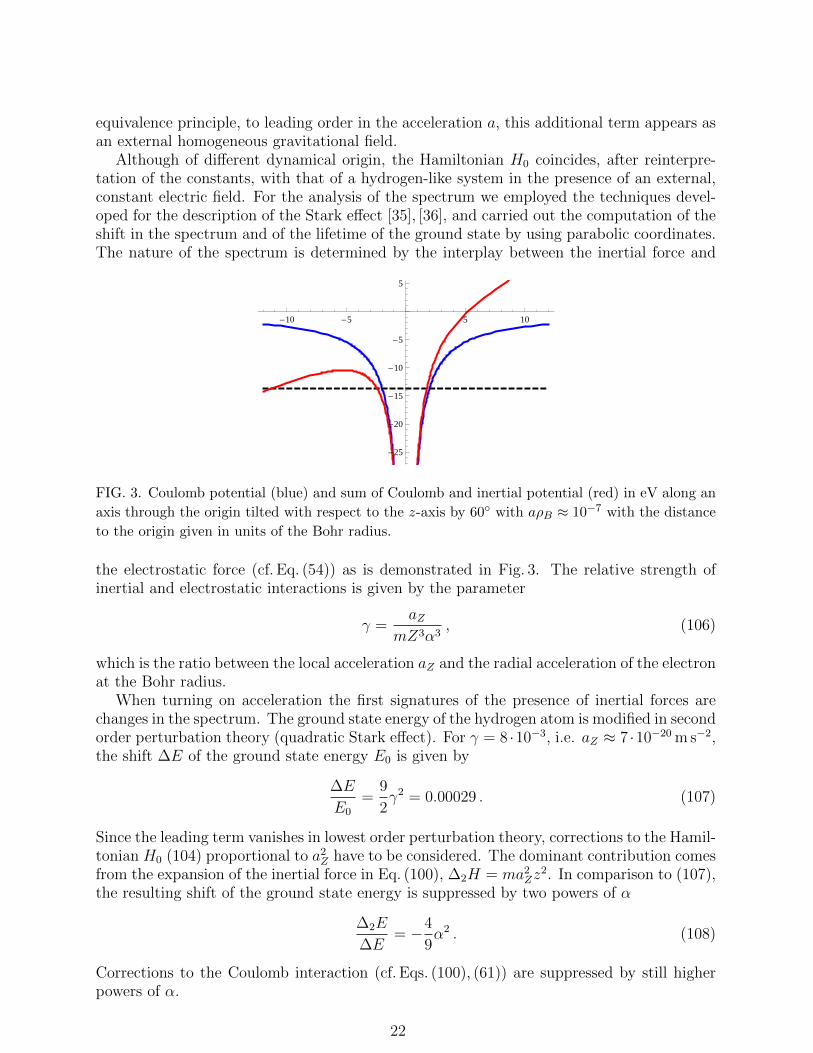
aZ. (111)

In Fig. 4 is shown the probability that an ensemble of hydrogen atoms has been ion-ized since the big bang as a function of the proper distance from the horizon e.g. froma Schwarzschild black hole. We note that only the value of the local acceleration aZ matters(cf. Eqs. (106), (110)) and therefore the curve shown in Fig. 4 is independent of the acceler-ation a, i.e. of the mass of the black hole. The transition from atoms to ions happens at adistance of about 10−4 m within an interval of the order of 10−5 m.

23

0.120 0.125 0.130 0.135 0.140 0.145

0.2

0.4

0.6

0.8

1.0

FIG. 4. Ionization probability of hydrogen atoms as a function of the distance to the horizon (111)

of a black hole.

In extending these arguments to other forms of matter we find that heavy atoms(cf. Eqs. (106), (110)) are ionized by the inertial force at a distance from the horizon ofthe order of 10−10 m. Using similar qualitative arguments based on the approximate iden-tity of inertial and the strong force in the region of “ionization”, ejection of a nucleon fromthe nucleus by acceleration is estimated to occur at a distance to the horizon of the order of10−13 m. However, in this case as well as for heavy atoms, the identification of the interac-tion in accelerated and inertial frames may become problematic. Since we expect the stronginteraction to be reduced by the inertial force as is the case for electrostatic interactions,these distances to the horizon are most likely underestimated. As for the atoms, no boundstates of nucleons can exist irrespective of the details of the nuclear force provided theacceleration has lasted for an infinitely long time. In turn, tunneling processes may also beimportant for the instability of nuclei.

As far as the stability of elementary particles are concerned which are subject to aninfinitely long lasting acceleration, related arguments can be put forward which indicatethat also in the presence of interactions their properties in Rindler space will remain to bequite different from those in Minkowski space. For illustration we consider a self-interactingscalar field which, depending on the interaction, may involve mass generation accompaniedby spontaneous symmetry breakdown. The Rindler space Hamiltonian of a self interactingscalar field is given by (cf. (10))

H =1

2

∫dξd2x⊥

π2 + (∂ξφ)2 + e2aξ

((∂⊥φ)2 + V (φ)

) (112)

with V chosen such that the minimum of V occurs for φ = ±φ0 6= 0. The expectationvalue φ0 of the scalar field generated by the self interaction obviously remains the same aftercarrying out the coordinate transformation from Minkowski to Rindler space (cf. [10] for adiscussion within the path integral approach). The implications of the symmetry breakingin Rindler space are not as obvious as in Minkowski space. Symmetry breaking with massgeneration does not leave signatures in the spectrum of the effective Hamiltonian in Rindlerspace. Furthermore as for non-interacting theories, in the presence of accelerated sourcesscalar particle production by acceleration in Minkowski space gives rise to on-shell zeroenergy particles present in Rindler space. A cloud of scalar on-shell particles is presentfor both massive and massless particles. On the other hand, we also cannot invoke therestoration of symmetry, when heating the system, as an argument for a phase transition

24

by increase of the acceleration a. A change in a not only changes the temperature but alsothe Hamiltonian (112). Thus it is not obvious that a non-vanishing φ0 also implies a changefrom the symmetric to the symmetry broken phase in the whole of Rindler space. Rather itseems plausible that, in analogy to the transition of an ensemble of atoms in Fig. 4, locallyeither the broken or the restored symmetry is realized depending on the distance from thehorizon. To be more specific we consider the standard φ4 potential and expand it aroundthe minimum at φ = φ0

V (φ) = V (ϕ, φ0) =λ

8φ2(φ2 − 2φ2

0) ≈ −λ8φ4

0 +m2

2ϕ2 , m2 = λφ2

0. (113)

Although formally the minimum in the potential energy V (φ) is attained at φ = φ0 inde-pendent of the value of ξ, it is also plausible that the relevance of this minimum dependson the value of ξ. It has been argued [38] that, for sufficiently small ξ, the potential V (φ)together with the transverse kinetic term can be neglected resulting in a reduction to anon-interacting massless 1+1 dimensional field theory. Here we give a rough estimate ofthe value of ξ where the effect of the potential V (φ) becomes negligible by equating thefluctuations in the energy density including those generated by the transverse motion

ε(ξ) = e−2aξ〈0M | : H(ξ,x⊥) : |0M〉 =e−2aξ

2〈0M | : π2 + (∂ξϕ)2 + e2aξ

((∂⊥ϕ)2 +m2ϕ

): |0M〉 .

(114)with the change in energy density associated with the local breaking of the reflection sym-metry φ→ −φ

ε(ξ) ≈ λ

8φ4

0 . (115)

The expectation value ε(ξ) is taken in the Minkowski space vacuum with the operatorH(ξ,x⊥) being normal ordered with respect to the Rindler space vacuum. Inserting thenormal mode expansion (9) and carrying out the k⊥ integration (cf. [22]) we obtain for theenergy density as a function of the distance to the horizon dH = eaξ/a (cf. Eq. (111))

ε(dH) =m2

4π3d2H

∫ ∞0

dχe−πχ

(χ2 + 1)[K1+iχ(mdH)K1−iχ(mdH)−

(Kiχ(mdH)

)2]

−1

2Kiχ(mdH)

[mdHK

′iχ(mdH)−Kiχ(mdH)

], (116)

where K ′iχ denotes the derivative with respect to the argument. Numerical evaluation ofthis integral shows that for mdH ≤ 0.2, the energy density agrees within 10% or less withthe m = 0 limit which can be calculated in closed form

ε(dH) ≈ 11

480π2d4H

. (117)

The energy densities associated with the symmetry breakdown and with the fluctuations areof the same order of magnitude for the following value of the distance to the horizon

dH ≈( 11

60 π2λ

) 14 1

φ0

. (118)

Identifying the parameters λ and φ0 with those of the Higgs potential of the standard model(with the Higgs mass 100 GeV ≤ m ≤ 250 GeV), Eq. (118) yields, in qualitative agreement

25

with the numerical evaluation of Eqs. (115) and (116), dH ≈ (4±1) ·10−19 m, i.e., we expectthat at these or smaller distances the presence of a non-vanishing expectation value of thescalar field will be irrelevant. The expression (117) for the variation in the energy densitycan also be interpreted as due to the spatial variation of the Tolman temperature

TTolman =1

2πdH. (119)

Up to numerical factors, the energy density (117) is that of a massless scalar field in 3+1dimensions at the temperature T = TTolman. The value TTolman ≈ 80 GeV is of the sameorder of magnitude as the critical temperature of the electroweak phase transition.

V. CONCLUSIONS

The focus of our studies of quantum fields in Rindler space has been on the forces whichare generated by exchange of massless bosons and are acting between sources at rest inRindler space. We have presented detailed results for exchange of scalar particles, photonsand gravitons. In comparison to Minkowski space, the most striking difference of the inter-action energies is the appearance of a non-trivial imaginary part in Rindler space. Unlike the(classical) real part of the interaction energy, the imaginary part is of quantum mechanicalorigin. The difference between real and imaginary contributions can be lucidly illustrated forphoton exchange. In Weyl gauge, longitudinal and transverse degrees of freedom are cleanlyseparated with the longitudinal field determining the real and the transverse photons theimaginary part.

In contrast to the universal 1/r behavior in Minkowski space, the real part of the interac-tion energies in Rindler space exhibits significant differences for the three cases considered.Independent of the spin of the exchanged particles is only the behavior of the forces at shortdistances where inertial forces are negligible and the leading terms agree with the Minkowskispace result. For large separations of the sources, the real part of the interaction energyof scalar sources is suppressed and the electrostatic interaction energy approaches a non-vanishing constant while a divergence is encountered for gravitational sources. Significantdifferences also appear when approaching the horizon akin to the differences which, in thecontext of the “no-hair” theorem, have been obtained close to the horizon of a Schwarzschildblack hole [30], [31], [32].

The existence of an imaginary contribution to the interaction energy is a direct conse-quence of the peculiar degeneracy of the spectrum of Rindler space particles and is there-fore of the same origin as the one-dimensional density of states appearing in the energy-momentum tensor of scalar or vector fields [37], [5]. The degeneracy is a consequence ofthe invariance of the Rindler space Hamiltonian under scale transformations as is the scaleinvariance of the static interaction energies. Of particular relevance for the static interac-tions is the degeneracy of the zero energy sector of the Rindler particles. The degeneracy ischaracterized by the values of the 2 momentum components transverse to the direction ofthe acceleration. The imaginary part is generated by emission, on-shell propagation and ab-sorption of zero energy Rindler particles and is directly related to the (zero energy) particlecreation and annihilation rates in Rindler space. This result, together with the connectionof “radiation” in Rindler and Minkowski spaces [6], [7], [8], implies that the imaginary partof the interaction energy in Rindler space is given by the rate of particle production of a

26

uniformly accelerated charge in Minkowski space, measured by the Rindler time. Thus con-sistency between the radiation observed in Minkowski space and the zero energy radiation inRindler space is established by the existence of a non-trivial zero energy sector which in turnrequires a symmetry which guarantees the degeneracy. Seen from this point of view it maynot come as a surprise that the symmetry under appropriately generalized scale transfor-mations persists [14] for massive particles and guarantees consistency between Rindler andMinkowski space formulations also in this case. While negligible for small separations ofthe two sources, the imaginary contribution dominates the force at large distances for scalarparticle and photon exchange. As the real part, also the imaginary part of the gravitationalinteraction is divergent. The counterpart of this divergence of the static graviton propaga-tor in Rindler space is the divergence of the energy momentum tensor of the “eternally”,uniformly accelerated mass point in Minkowski space. This divergence indicates that theimplicit assumption of a negligible backreaction on the gravitational field is invalid.

The weakening of the interaction for scalar particle and photon exchange as well as theappearance of a non-trivial imaginary contribution point to instability of matter in Rindlerspace. We have confirmed this instability in a calculation of the rate of ionization of hydrogenatoms at rest as a function of the distance from the horizon or equivalently of the Tolmantemperature. Similar arguments point to the instability of nuclear matter which will set inat significantly smaller distances to the horizon. In this hierarchy of instability one mayalso expect, at still smaller distances, instability of the phases of matter determined by thedynamics of quantum fields. Within the context of a self-interacting scalar field we haveshown that the strength of the fluctuations increases when approaching the horizon andwe have determined the distance where the fluctuations and the mean field generated bysymmetry breaking contribute equally to the energy density. At still smaller distances, mostlikely the expectation value of the scalar field becomes irrelevant for the dynamics. Usingparameters of the standard model, the corresponding Tolman temperature has been foundto be of the same order of magnitude as the temperature of the electroweak phase transition.Of interest in this context is the issue of a possible confinement-deconfinement transitionwhen approaching the horizon. As in Minkowski space, this issue most likely has to besettled in numerical simulations. The strong force will have to be determined in calculationsof the Polyakov loop correlation functions on a lattice in Rindler space with imaginary time.As in the electrostatic case the interaction energy determined in this way will be a realquantity. Whether confinement in Rindler space implies a vanishing imaginary contributionto the force or the imaginary part can be reconstructed, on the basis of the numericallydetermined spectrum and correlation functions, has to be clarified.

ACKNOWLEDGMENTS

F.L. is grateful for the support and the hospitality at the En’yo Radiation Laboratoryand the Hashimoto Mathematical Physics Laboratory of the Nishina Accelerator ResearchCenter at RIKEN. This work is supported in part by the Grant-in-Aid for Scientific Researchfrom MEXT (No. 22540302).

[1] S. A. Fulling, Phys. Rev. D 7, (1973), 2850

27

[2] D. G. Boulware, Phys. Rev. D 11, (1975), 1404

[3] P. C. W. Davies, J. Phys. A 8, (1975), 609

[4] W. G. Unruh, Phys. Rev. D 14, (1976), 870

[5] W. D. Sciama, P. Candelas and D. Deutsch, Adv. in Phys. 30, (1981), 327

[6] A. Higuchi, G. E. A. Matsas and D. Sudarsky, Phys. Rev. D 45, (1992), R3308

[7] A. Higuchi, G. E. A. Matsas and D. Sudarsky, Phys. Rev. D 46, (1992), 3450

[8] H. Ren and E. J. Weinberg, Phys. Rev. D 49, (1994), 6526, [arXiv:hep-th/9312038]

[9] L. C. B. Crispino, A. Higuchi and G. E. A. Matsas, Rev. Mod. Phys. 80, (2008), 787, [arXiv:gr-

qc/0710.5373]

[10] W. G. Unruh and N. Weiss, Phys. Rev. D 29, (1984), 1656

[11] R. Passante, Phys. Rev. A 57, (1998), 1590

[12] R. Muller, Phys. Rev. D 56, (1997), 953

[13] D. A. T. Vanzella and G. E. A. Matsas, Phys. Rev. D 63, (2000), 014010, [arXiv:hep-

th/0002010]

[14] F. Lenz, K. Ohta and K. Yazaki, Phys. Rev. D 78, (2008), 065026, [arXiv:hep-th/0803.2001]

[15] W. Rindler, Relativity, Special, General and Cosmological, Oxford University Press, 2001

[16] W. Trost and H. Van Dam, Phys. Lett. B 71, (1977), 149 and Nucl. Phys. B 152, (1979), 442

[17] J. S. Dowker, Phys. Rev. D 18, (1978), 1856

[18] S. M. Christensen and M. J. Duff, Nucl. Phys. B 146, (1978), 11

[19] B. Linet, [arXiv:gr-qc/9505033]

[20] N. F. Svaiter ans C. A. D. Zarro, Class. Quant. Grav. 25, (2008), 095008

[21] P. Candelas and D. J. Raine, J. Math. Phys. 17, (1976), 2101

[22] I. S. Gradshteyn and I. M. Ryzhik, Table of Integrals, Series and Products, Academic Press

1965

[23] A. Erdelyi, W. Magnus, F. Oberhettinger and F. G. Tricomi, Higher Transcendental Functions,

Vol. I, McGraw Hill 1953

[24] P. G. Grove, Class. Quant. Grav. 3, (1986), 801

[25] S. Massar, R. Parentani and R. Brout, Class. Quant. Grav. 10, (1993), 385

[26] W. G. Unruh, Phys. Rev. D 46, (1992), 3271

[27] B. L. Hu and A. Raval, [arXiv:quant/ph 0012134]

[28] J. Baez & J. P. Muniain, Gauge Fields, Knots and Gravity, World Scientific, 1994

[29] J. Smit, Introduction to Quantum Fields on a Lattice, Cambridge University Press, 2002

[30] J. D. Bekenstein, Phys. Rev. Lett. 28, (1972), 452

[31] J. D. Bekenstein, Black Holes: Classical Properties, Thermodynamics and Heuristic Quanti-

zation, in: Cosmology and Gravitation, Atlanticsciences, M. Novello (Ed.) p. 1

[32] C. Teitelboim, Phys. Rev. D 5, (1972), 2951

[33] J. M. Cohen and R. M. Wald, J. Math. Phys. 12, (1971), 1845

[34] M. Wald, Commun. Math. Phys. 70, (1979), 221

[35] H. A. Bethe and E. E. Salpeter, Quantum mechanics of one- and two-electron atoms, Springer

Verlag, 1957

[36] K.-I. Hiraizumi, Y. Y. Ohshima and H. Suzuki, Phys. Lett. A 216, (1996), 117

[37] P. Candelas and D. Deutsch, Proc. R. Soc. Lond. A 354, (1977), 79

[38] T. Padmanabhan, Rep. Prog. Phys. 73, (2010), 046901 [arXiv:gr-qc/0911.5004]

28