F AIRLab, Politecnico di Milano arXiv:1603.07285v2 … · A guide to convolution arithmetic for...
31
A guide to convolution arithmetic for deep learning Vincent Dumoulin 1F and Francesco Visin 2F† F MILA, Université de Montréal † AIRLab, Politecnico di Milano January 12, 2018 1 [email protected] 2 [email protected] arXiv:1603.07285v2 [stat.ML] 11 Jan 2018
Transcript of F AIRLab, Politecnico di Milano arXiv:1603.07285v2 … · A guide to convolution arithmetic for...
A guide to convolution arithmetic for deeplearning
Vincent Dumoulin1F and Francesco Visin2F†
FMILA, Université de Montréal†AIRLab, Politecnico di Milano
January 12, 2018
[email protected]@polimi.it
arX
iv:1
603.
0728
5v2
[st
at.M
L]
11
Jan
2018

All models are wrong, but someare useful.
George E. P. Box
2

Acknowledgements
The authors of this guide would like to thank David Warde-Farley,Guillaume Alain and Caglar Gulcehre for their valuable feedback. Weare likewise grateful to all those who helped improve this tutorial withhelpful comments, constructive criticisms and code contributions. Keepthem coming!
Special thanks to Ethan Schoonover, creator of the Solarized colorscheme,1 whose colors were used for the figures.
Feedback
Your feedback is welcomed! We did our best to be as precise, infor-mative and up to the point as possible, but should there be anything youfeel might be an error or could be rephrased to be more precise or com-prehensible, please don’t refrain from contacting us. Likewise, drop us aline if you think there is something that might fit this technical reportand you would like us to discuss – we will make our best effort to updatethis document.
Source code and animations
The code used to generate this guide along with its figures is availableon GitHub.2 There the reader can also find an animated version of thefigures.
1http://ethanschoonover.com/solarized2https://github.com/vdumoulin/conv_arithmetic
3

Contents
1 Introduction 51.1 Discrete convolutions . . . . . . . . . . . . . . . . . . . . . . . . . 61.2 Pooling . . . . . . . . . . . . . . . . . . . . . . . . . . . . . . . . 10
2 Convolution arithmetic 122.1 No zero padding, unit strides . . . . . . . . . . . . . . . . . . . . 122.2 Zero padding, unit strides . . . . . . . . . . . . . . . . . . . . . . 13
2.2.1 Half (same) padding . . . . . . . . . . . . . . . . . . . . . 132.2.2 Full padding . . . . . . . . . . . . . . . . . . . . . . . . . 13
2.3 No zero padding, non-unit strides . . . . . . . . . . . . . . . . . . 152.4 Zero padding, non-unit strides . . . . . . . . . . . . . . . . . . . . 15
3 Pooling arithmetic 18
4 Transposed convolution arithmetic 194.1 Convolution as a matrix operation . . . . . . . . . . . . . . . . . 204.2 Transposed convolution . . . . . . . . . . . . . . . . . . . . . . . 204.3 No zero padding, unit strides, transposed . . . . . . . . . . . . . 214.4 Zero padding, unit strides, transposed . . . . . . . . . . . . . . . 22
4.4.1 Half (same) padding, transposed . . . . . . . . . . . . . . 224.4.2 Full padding, transposed . . . . . . . . . . . . . . . . . . . 22
4.5 No zero padding, non-unit strides, transposed . . . . . . . . . . . 244.6 Zero padding, non-unit strides, transposed . . . . . . . . . . . . . 24
5 Miscellaneous convolutions 285.1 Dilated convolutions . . . . . . . . . . . . . . . . . . . . . . . . . 28
4
Chapter 1
Introduction
Deep convolutional neural networks (CNNs) have been at the heart of spectac-ular advances in deep learning. Although CNNs have been used as early as thenineties to solve character recognition tasks (Le Cun et al., 1997), their currentwidespread application is due to much more recent work, when a deep CNNwas used to beat state-of-the-art in the ImageNet image classification challenge(Krizhevsky et al., 2012).
Convolutional neural networks therefore constitute a very useful tool for ma-chine learning practitioners. However, learning to use CNNs for the first timeis generally an intimidating experience. A convolutional layer’s output shapeis affected by the shape of its input as well as the choice of kernel shape, zeropadding and strides, and the relationship between these properties is not triv-ial to infer. This contrasts with fully-connected layers, whose output size isindependent of the input size. Additionally, CNNs also usually feature a pool-ing stage, adding yet another level of complexity with respect to fully-connectednetworks. Finally, so-called transposed convolutional layers (also known as frac-tionally strided convolutional layers) have been employed in more and more workas of late (Zeiler et al., 2011; Zeiler and Fergus, 2014; Long et al., 2015; Rad-ford et al., 2015; Visin et al., 2015; Im et al., 2016), and their relationship withconvolutional layers has been explained with various degrees of clarity.
This guide’s objective is twofold:
1. Explain the relationship between convolutional layers and transposed con-volutional layers.
2. Provide an intuitive understanding of the relationship between input shape,kernel shape, zero padding, strides and output shape in convolutional,pooling and transposed convolutional layers.
In order to remain broadly applicable, the results shown in this guide areindependent of implementation details and apply to all commonly used machinelearning frameworks, such as Theano (Bergstra et al., 2010; Bastien et al., 2012),
5
Torch (Collobert et al., 2011), Tensorflow (Abadi et al., 2015) and Caffe (Jiaet al., 2014).
This chapter briefly reviews the main building blocks of CNNs, namely dis-crete convolutions and pooling. For an in-depth treatment of the subject, seeChapter 9 of the Deep Learning textbook (Goodfellow et al., 2016).
1.1 Discrete convolutionsThe bread and butter of neural networks is affine transformations: a vectoris received as input and is multiplied with a matrix to produce an output (towhich a bias vector is usually added before passing the result through a non-linearity). This is applicable to any type of input, be it an image, a soundclip or an unordered collection of features: whatever their dimensionality, theirrepresentation can always be flattened into a vector before the transformation.
Images, sound clips and many other similar kinds of data have an intrinsicstructure. More formally, they share these important properties:
• They are stored as multi-dimensional arrays.
• They feature one or more axes for which ordering matters (e.g., width andheight axes for an image, time axis for a sound clip).
• One axis, called the channel axis, is used to access different views of thedata (e.g., the red, green and blue channels of a color image, or the leftand right channels of a stereo audio track).
These properties are not exploited when an affine transformation is applied;in fact, all the axes are treated in the same way and the topological informationis not taken into account. Still, taking advantage of the implicit structure ofthe data may prove very handy in solving some tasks, like computer vision andspeech recognition, and in these cases it would be best to preserve it. This iswhere discrete convolutions come into play.
A discrete convolution is a linear transformation that preserves this notionof ordering. It is sparse (only a few input units contribute to a given outputunit) and reuses parameters (the same weights are applied to multiple locationsin the input).
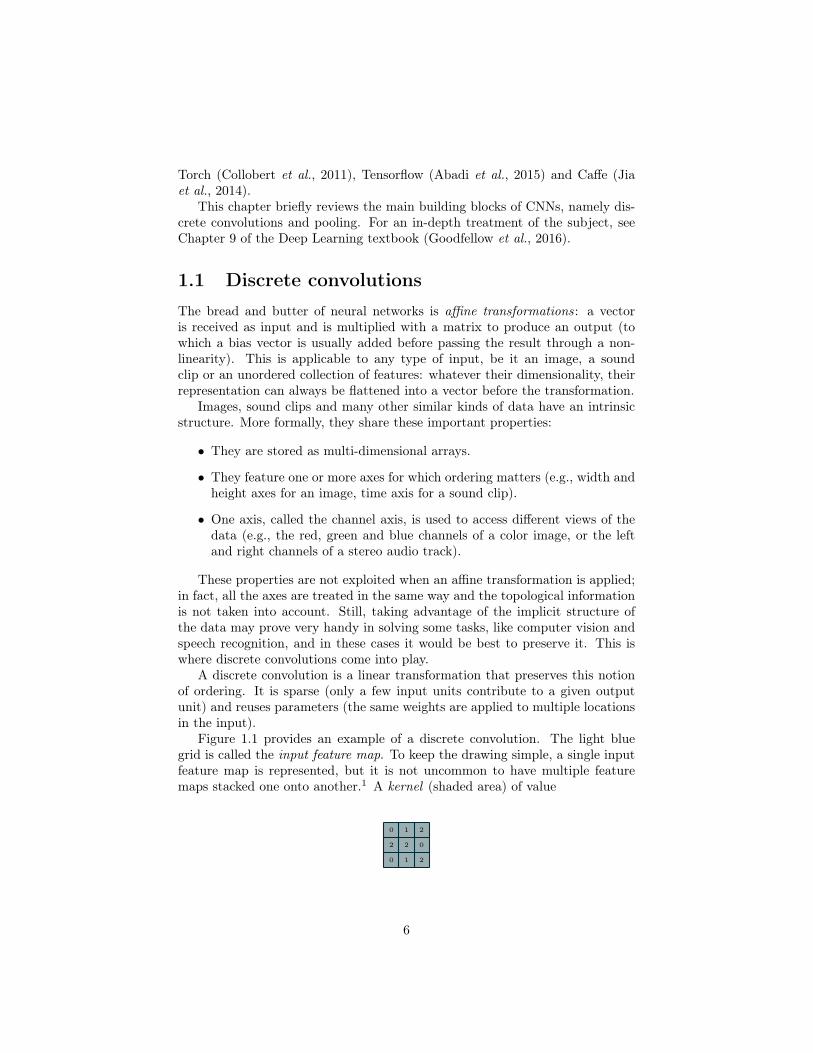
Figure 1.1 provides an example of a discrete convolution. The light bluegrid is called the input feature map. To keep the drawing simple, a single inputfeature map is represented, but it is not uncommon to have multiple featuremaps stacked one onto another.1 A kernel (shaded area) of value
0 1 2
2 2 0
0 1 2
6

2
2
3
0
3
0
0
1
0
3
0
0
2
1
2
0
2
2
3
1
1
2
3
1
0
0
2
0
1
2
1
2
0
2
9.0
10.0
12.0
6.0
17.0
12.0
14.0
19.0
17.0
2
2
3
0
3
0
0
1
0
3
0
0
2
1
2
0
2
2
3
1
1
2
3
1
0
0
2
0
1
2
1
2
0
2
9.0
10.0
12.0
6.0
17.0
12.0
14.0
19.0
17.0
2
2
3
0
3
0
0
1
0
3
0
0
2
1
2
0
2
2
3
1
1
2
3
1
0
0
2
0
1
2
1
2
0
2
9.0
10.0
12.0
6.0
17.0
12.0
14.0
19.0
17.0
2
2
3
0
3
0
0
1
0
3
0
0
2
1
2
0
2
2
3
1
1
2
3
1
0
0
2
0
1
2
1
2
0
2
9.0
10.0
12.0
6.0
17.0
12.0
14.0
19.0
17.0
2
2
3
0
3
0
0
1
0
3
0
0
2
1
2
0
2
2
3
1
1
2
3
1
0
0
2
0
1
2
1
2
0
2
9.0
10.0
12.0
6.0
17.0
12.0
14.0
19.0
17.0
2
2
3
0
3
0
0
1
0
3
0
0
2
1
2
0
2
2
3
1
1
2
3
1
0
0
2
0
1
2
1
2
0
2
9.0
10.0
12.0
6.0
17.0
12.0
14.0
19.0
17.0
2
2
3
0
3
0
0
1
0
3
0
0
2
1
2
0
2
2
3
1
1
2
3
1
0
0
2
0
1
2
1
2
0
2
9.0
10.0
12.0
6.0
17.0
12.0
14.0
19.0
17.0
2
2
3
0
3
0
0
1
0
3
0
0
2
1
2
0
2
2
3
1
1
2
3
1
0
0
2
0
1
2
1
2
0
2
9.0
10.0
12.0
6.0
17.0
12.0
14.0
19.0
17.0
2
2
3
0
3
0
0
1
0
3
0
0
2
1
2
0
2
2
3
1
1
2
3
1
0
0
2
0
1
2
1
2
0
2
9.0
10.0
12.0
6.0
17.0
12.0
14.0
19.0
17.0
Figure 1.1: Computing the output values of a discrete convolution.
0
0
0
0
0
0
0
0
2
2
3
0
3
0
0
0
0
1
0
3
0
0
0
0
2
1
2
0
0
0
2
2
3
1
0
0
1
2
3
1
0
0
0
0
0
0
0
0
0
0
2
0
1
2
1
2
0
2
6.0
8.0
6.0
4.0
17.0
17.0
4.0
13.0
3.0
0
0
0
0
0
0
0
0
2
2
3
0
3
0
0
0
0
1
0
3
0
0
0
0
2
1
2
0
0
0
2
2
3
1
0
0
1
2
3
1
0
0
0
0
0
0
0
0
0
0
2
0
1
2
1
2
0
2
6.0
8.0
6.0
4.0
17.0
17.0
4.0
13.0
3.0
0
0
0
0
0
0
0
0
2
2
3
0
3
0
0
0
0
1
0
3
0
0
0
0
2
1
2
0
0
0
2
2
3
1
0
0
1
2
3
1
0
0
0
0
0
0
0
0
0
0
2
0
1
2
1
2
0
2
6.0
8.0
6.0
4.0
17.0
17.0
4.0
13.0
3.0
0
0
0
0
0
0
0
0
2
2
3
0
3
0
0
0
0
1
0
3
0
0
0
0
2
1
2
0
0
0
2
2
3
1
0
0
1
2
3
1
0
0
0
0
0
0
0
0
0
0
2
0
1
2
1
2
0
2
6.0
8.0
6.0
4.0
17.0
17.0
4.0
13.0
3.0
0
0
0
0
0
0
0
0
2
2
3
0
3
0
0
0
0
1
0
3
0
0
0
0
2
1
2
0
0
0
2
2
3
1
0
0
1
2
3
1
0
0
0
0
0
0
0
0
0
0
2
0
1
2
1
2
0
2
6.0
8.0
6.0
4.0
17.0
17.0
4.0
13.0
3.0
0
0
0
0
0
0
0
0
2
2
3
0
3
0
0
0
0
1
0
3
0
0
0
0
2
1
2
0
0
0
2
2
3
1
0
0
1
2
3
1
0
0
0
0
0
0
0
0
0
0
2
0
1
2
1
2
0
2
6.0
8.0
6.0
4.0
17.0
17.0
4.0
13.0
3.0
0
0
0
0
0
0
0
0
2
2
3
0
3
0
0
0
0
1
0
3
0
0
0
0
2
1
2
0
0
0
2
2
3
1
0
0
1
2
3
1
0
0
0
0
0
0
0
0
0
0
2
0
1
2
1
2
0
26.0
8.0
6.0
4.0
17.0
17.0
4.0
13.0
3.0
0
0
0
0
0
0
0
0
2
2
3
0
3
0
0
0
0
1
0
3
0
0
0
0
2
1
2
0
0
0
2
2
3
1
0
0
1
2
3
1
0
0
0
0
0
0
0
0
0
0
2
0
1
2
1
2
0
26.0
8.0
6.0
4.0
17.0
17.0
4.0
13.0
3.0
0
0
0
0
0
0
0
0
2
2
3
0
3
0
0
0
0
1
0
3
0
0
0
0
2
1
2
0
0
0
2
2
3
1
0
0
1
2
3
1
0
0
0
0
0
0
0
0
0
0
2
0
1
2
1
2
0
26.0
8.0
6.0
4.0
17.0
17.0
4.0
13.0
3.0
Figure 1.2: Computing the output values of a discrete convolution for N = 2,i1 = i2 = 5, k1 = k2 = 3, s1 = s2 = 2, and p1 = p2 = 1.
7

slides across the input feature map. At each location, the product betweeneach element of the kernel and the input element it overlaps is computed andthe results are summed up to obtain the output in the current location. Theprocedure can be repeated using different kernels to form as many output featuremaps as desired (Figure 1.3). The final outputs of this procedure are calledoutput feature maps.2 If there are multiple input feature maps, the kernel willhave to be 3-dimensional – or, equivalently each one of the feature maps willbe convolved with a distinct kernel – and the resulting feature maps will besummed up elementwise to produce the output feature map.
The convolution depicted in Figure 1.1 is an instance of a 2-D convolution,but it can be generalized to N-D convolutions. For instance, in a 3-D convolu-tion, the kernel would be a cuboid and would slide across the height, width anddepth of the input feature map.
The collection of kernels defining a discrete convolution has a shape corre-sponding to some permutation of (n,m, k1, . . . , kN ), where
n ≡ number of output feature maps,m ≡ number of input feature maps,kj ≡ kernel size along axis j.
The following properties affect the output size oj of a convolutional layeralong axis j:
• ij : input size along axis j,
• kj : kernel size along axis j,
• sj : stride (distance between two consecutive positions of the kernel) alongaxis j,
• pj : zero padding (number of zeros concatenated at the beginning and atthe end of an axis) along axis j.
For instance, Figure 1.2 shows a 3 × 3 kernel applied to a 5 × 5 input paddedwith a 1× 1 border of zeros using 2× 2 strides.
Note that strides constitute a form of subsampling. As an alternative tobeing interpreted as a measure of how much the kernel is translated, strides canalso be viewed as how much of the output is retained. For instance, movingthe kernel by hops of two is equivalent to moving the kernel by hops of one butretaining only odd output elements (Figure 1.4).
1An example of this is what was referred to earlier as channels for images and sound clips.2While there is a distinction between convolution and cross-correlation from a signal pro-
cessing perspective, the two become interchangeable when the kernel is learned. For the sakeof simplicity and to stay consistent with most of the machine learning literature, the termconvolution will be used in this guide.
8

+ + +
Figure 1.3: A convolution mapping from two input feature maps to three outputfeature maps using a 3× 2× 3× 3 collection of kernels w. In the left pathway,input feature map 1 is convolved with kernel w1,1 and input feature map 2 isconvolved with kernel w1,2, and the results are summed together elementwiseto form the first output feature map. The same is repeated for the middle andright pathways to form the second and third feature maps, and all three outputfeature maps are grouped together to form the output.
Figure 1.4: An alternative way of viewing strides. Instead of translating the3× 3 kernel by increments of s = 2 (left), the kernel is translated by incrementsof 1 and only one in s = 2 output elements is retained (right).
9

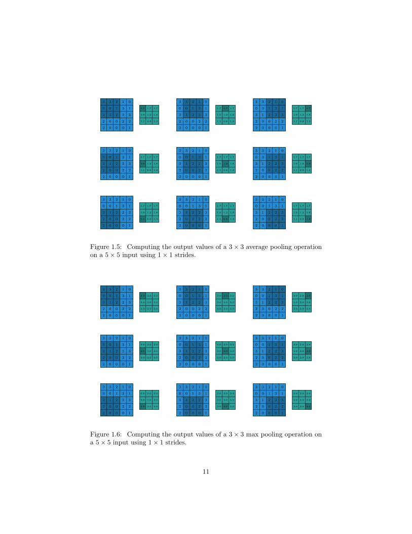
1.2 PoolingIn addition to discrete convolutions themselves, pooling operations make upanother important building block in CNNs. Pooling operations reduce the sizeof feature maps by using some function to summarize subregions, such as takingthe average or the maximum value.
Pooling works by sliding a window across the input and feeding the contentof the window to a pooling function. In some sense, pooling works very muchlike a discrete convolution, but replaces the linear combination described by thekernel with some other function. Figure 1.5 provides an example for averagepooling, and Figure 1.6 does the same for max pooling.
The following properties affect the output size oj of a pooling layer alongaxis j:
• ij : input size along axis j,
• kj : pooling window size along axis j,
• sj : stride (distance between two consecutive positions of the pooling win-dow) along axis j.
10
2
2
3
0
3
0
0
1
0
3
0
0
2
1
2
0
2
2
3
1
1
2
3
1
0
1.1
1.0
1.7
0.8
1.2
1.7
1.3
1.8
1.7
2
2
3
0
3
0
0
1
0
3
0
0
2
1
2
0
2
2
3
1
1
2
3
1
0
1.1
1.0
1.7
0.8
1.2
1.7
1.3
1.8
1.7
2
2
3
0
3
0
0
1
0
3
0
0
2
1
2
0
2
2
3
1
1
2
3
1
0
1.1
1.0
1.7
0.8
1.2
1.7
1.3
1.8
1.7
2
2
3
0
3
0
0
1
0
3
0
0
2
1
2
0
2
2
3
1
1
2
3
1
0
1.1
1.0
1.7
0.8
1.2
1.7
1.3
1.8
1.7
2
2
3
0
3
0
0
1
0
3
0
0
2
1
2
0
2
2
3
1
1
2
3
1
0
1.1
1.0
1.7
0.8
1.2
1.7
1.3
1.8
1.7
2
2
3
0
3
0
0
1
0
3
0
0
2
1
2
0
2
2
3
1
1
2
3
1
0
1.1
1.0
1.7
0.8
1.2
1.7
1.3
1.8
1.7
2
2
3
0
3
0
0
1
0
3
0
0
2
1
2
0
2
2
3
1
1
2
3
1
0
1.1
1.0
1.7
0.8
1.2
1.7
1.3
1.8
1.7
2
2
3
0
3
0
0
1
0
3
0
0
2
1
2
0
2
2
3
1
1
2
3
1
0
1.1
1.0
1.7
0.8
1.2
1.7
1.3
1.8
1.7
2
2
3
0
3
0
0
1
0
3
0
0
2
1
2
0
2
2
3
1
1
2
3
1
0
1.1
1.0
1.7
0.8
1.2
1.7
1.3
1.8
1.7
Figure 1.5: Computing the output values of a 3× 3 average pooling operationon a 5× 5 input using 1× 1 strides.
2
2
3
0
3
0
0
1
0
3
0
0
2
1
2
0
2
2
3
1
1
2
3
1
0
3.0
3.0
3.0
2.0
3.0
3.0
3.0
3.0
3.0
2
2
3
0
3
0
0
1
0
3
0
0
2
1
2
0
2
2
3
1
1
2
3
1
0
3.0
3.0
3.0
2.0
3.0
3.0
3.0
3.0
3.0
2
2
3
0
3
0
0
1
0
3
0
0
2
1
2
0
2
2
3
1
1
2
3
1
0
3.0
3.0
3.0
2.0
3.0
3.0
3.0
3.0
3.0
2
2
3
0
3
0
0
1
0
3
0
0
2
1
2
0
2
2
3
1
1
2
3
1
0
3.0
3.0
3.0
2.0
3.0
3.0
3.0
3.0
3.0
2
2
3
0
3
0
0
1
0
3
0
0
2
1
2
0
2
2
3
1
1
2
3
1
0
3.0
3.0
3.0
2.0
3.0
3.0
3.0
3.0
3.0
2
2
3
0
3
0
0
1
0
3
0
0
2
1
2
0
2
2
3
1
1
2
3
1
0
3.0
3.0
3.0
2.0
3.0
3.0
3.0
3.0
3.0
2
2
3
0
3
0
0
1
0
3
0
0
2
1
2
0
2
2
3
1
1
2
3
1
0
3.0
3.0
3.0
2.0
3.0
3.0
3.0
3.0
3.0
2
2
3
0
3
0
0
1
0
3
0
0
2
1
2
0
2
2
3
1
1
2
3
1
0
3.0
3.0
3.0
2.0
3.0
3.0
3.0
3.0
3.0
2
2
3
0
3
0
0
1
0
3
0
0
2
1
2
0
2
2
3
1
1
2
3
1
0
3.0
3.0
3.0
2.0
3.0
3.0
3.0
3.0
3.0
Figure 1.6: Computing the output values of a 3× 3 max pooling operation ona 5× 5 input using 1× 1 strides.
11

Chapter 2
Convolution arithmetic
The analysis of the relationship between convolutional layer properties is easedby the fact that they don’t interact across axes, i.e., the choice of kernel size,stride and zero padding along axis j only affects the output size of axis j.Because of that, this chapter will focus on the following simplified setting:
• 2-D discrete convolutions (N = 2),
• square inputs (i1 = i2 = i),
• square kernel size (k1 = k2 = k),
• same strides along both axes (s1 = s2 = s),
• same zero padding along both axes (p1 = p2 = p).
This facilitates the analysis and the visualization, but keep in mind that theresults outlined here also generalize to the N-D and non-square cases.
2.1 No zero padding, unit stridesThe simplest case to analyze is when the kernel just slides across every positionof the input (i.e., s = 1 and p = 0). Figure 2.1 provides an example for i = 4and k = 3.
One way of defining the output size in this case is by the number of possibleplacements of the kernel on the input. Let’s consider the width axis: the kernelstarts on the leftmost part of the input feature map and slides by steps of oneuntil it touches the right side of the input. The size of the output will be equalto the number of steps made, plus one, accounting for the initial position of thekernel (Figure 2.8a). The same logic applies for the height axis.
More formally, the following relationship can be inferred:
12
Relationship 1. For any i and k, and for s = 1 and p = 0,
o = (i− k) + 1.
2.2 Zero padding, unit stridesTo factor in zero padding (i.e., only restricting to s = 1), let’s consider its effecton the effective input size: padding with p zeros changes the effective input sizefrom i to i + 2p. In the general case, Relationship 1 can then be used to inferthe following relationship:
Relationship 2. For any i, k and p, and for s = 1,
o = (i− k) + 2p+ 1.
Figure 2.2 provides an example for i = 5, k = 4 and p = 2.In practice, two specific instances of zero padding are used quite extensively
because of their respective properties. Let’s discuss them in more detail.
2.2.1 Half (same) paddingHaving the output size be the same as the input size (i.e., o = i) can be adesirable property:
Relationship 3. For any i and for k odd (k = 2n + 1, n ∈ N),s = 1 and p = bk/2c = n,
o = i+ 2bk/2c − (k − 1)
= i+ 2n− 2n
= i.
This is sometimes referred to as half (or same) padding. Figure 2.3 provides anexample for i = 5, k = 3 and (therefore) p = 1.
2.2.2 Full paddingWhile convolving a kernel generally decreases the output size with respect tothe input size, sometimes the opposite is required. This can be achieved withproper zero padding:
Relationship 4. For any i and k, and for p = k − 1 and s = 1,
o = i+ 2(k − 1)− (k − 1)
= i+ (k − 1).
13
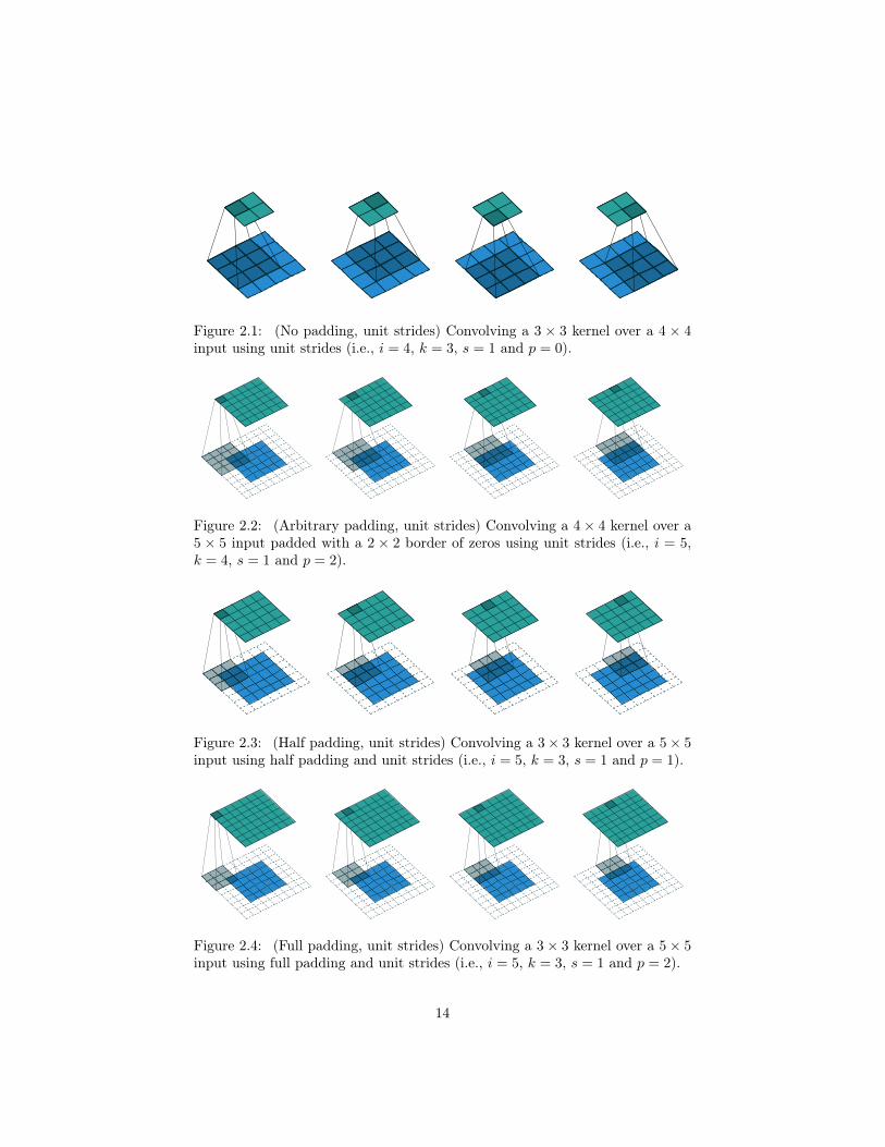
Figure 2.1: (No padding, unit strides) Convolving a 3 × 3 kernel over a 4 × 4input using unit strides (i.e., i = 4, k = 3, s = 1 and p = 0).
Figure 2.2: (Arbitrary padding, unit strides) Convolving a 4× 4 kernel over a5 × 5 input padded with a 2 × 2 border of zeros using unit strides (i.e., i = 5,k = 4, s = 1 and p = 2).
Figure 2.3: (Half padding, unit strides) Convolving a 3× 3 kernel over a 5× 5input using half padding and unit strides (i.e., i = 5, k = 3, s = 1 and p = 1).
Figure 2.4: (Full padding, unit strides) Convolving a 3× 3 kernel over a 5× 5input using full padding and unit strides (i.e., i = 5, k = 3, s = 1 and p = 2).
14

This is sometimes referred to as full padding, because in this setting everypossible partial or complete superimposition of the kernel on the input featuremap is taken into account. Figure 2.4 provides an example for i = 5, k = 3 and(therefore) p = 2.
2.3 No zero padding, non-unit stridesAll relationships derived so far only apply for unit-strided convolutions. In-corporating non unitary strides requires another inference leap. To facilitatethe analysis, let’s momentarily ignore zero padding (i.e., s > 1 and p = 0).Figure 2.5 provides an example for i = 5, k = 3 and s = 2.
Once again, the output size can be defined in terms of the number of possibleplacements of the kernel on the input. Let’s consider the width axis: the kernelstarts as usual on the leftmost part of the input, but this time it slides by stepsof size s until it touches the right side of the input. The size of the output isagain equal to the number of steps made, plus one, accounting for the initialposition of the kernel (Figure 2.8b). The same logic applies for the height axis.
From this, the following relationship can be inferred:
Relationship 5. For any i, k and s, and for p = 0,
o =
⌊i− k
s
⌋+ 1.
The floor function accounts for the fact that sometimes the last possible stepdoes not coincide with the kernel reaching the end of the input, i.e., some inputunits are left out (see Figure 2.7 for an example of such a case).
2.4 Zero padding, non-unit stridesThe most general case (convolving over a zero padded input using non-unitstrides) can be derived by applying Relationship 5 on an effective input of sizei+ 2p, in analogy to what was done for Relationship 2:
Relationship 6. For any i, k, p and s,
o =
⌊i+ 2p− k
s
⌋+ 1.
As before, the floor function means that in some cases a convolution will producethe same output size for multiple input sizes. More specifically, if i+ 2p− k isa multiple of s, then any input size j = i+ a, a ∈ {0, . . . , s− 1} will producethe same output size. Note that this ambiguity applies only for s > 1.
Figure 2.6 shows an example with i = 5, k = 3, s = 2 and p = 1, whileFigure 2.7 provides an example for i = 6, k = 3, s = 2 and p = 1. Interestingly,
15

despite having different input sizes these convolutions share the same outputsize. While this doesn’t affect the analysis for convolutions, this will complicatethe analysis in the case of transposed convolutions.
16

Figure 2.5: (No zero padding, arbitrary strides) Convolving a 3× 3 kernel overa 5× 5 input using 2× 2 strides (i.e., i = 5, k = 3, s = 2 and p = 0).
Figure 2.6: (Arbitrary padding and strides) Convolving a 3 × 3 kernel over a5× 5 input padded with a 1× 1 border of zeros using 2× 2 strides (i.e., i = 5,k = 3, s = 2 and p = 1).
Figure 2.7: (Arbitrary padding and strides) Convolving a 3 × 3 kernel over a6× 6 input padded with a 1× 1 border of zeros using 2× 2 strides (i.e., i = 6,k = 3, s = 2 and p = 1). In this case, the bottom row and right column of thezero padded input are not covered by the kernel.
(a) The kernel has to slide two stepsto the right to touch the right side ofthe input (and equivalently downwards).Adding one to account for the initial ker-nel position, the output size is 3× 3.
(b) The kernel has to slide one step ofsize two to the right to touch the rightside of the input (and equivalently down-wards). Adding one to account for theinitial kernel position, the output size is2× 2.
Figure 2.8: Counting kernel positions.
17
Chapter 3
Pooling arithmetic
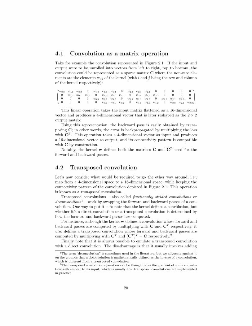
In a neural network, pooling layers provide invariance to small translations ofthe input. The most common kind of pooling is max pooling, which consistsin splitting the input in (usually non-overlapping) patches and outputting themaximum value of each patch. Other kinds of pooling exist, e.g., mean oraverage pooling, which all share the same idea of aggregating the input locallyby applying a non-linearity to the content of some patches (Boureau et al.,2010a,b, 2011; Saxe et al., 2011).
Some readers may have noticed that the treatment of convolution arithmeticonly relies on the assumption that some function is repeatedly applied ontosubsets of the input. This means that the relationships derived in the previouschapter can be reused in the case of pooling arithmetic. Since pooling does notinvolve zero padding, the relationship describing the general case is as follows:
Relationship 7. For any i, k and s,
o =
⌊i− k
s
⌋+ 1.
This relationship holds for any type of pooling.
18

Chapter 4
Transposed convolutionarithmetic
The need for transposed convolutions generally arises from the desire to use atransformation going in the opposite direction of a normal convolution, i.e., fromsomething that has the shape of the output of some convolution to somethingthat has the shape of its input while maintaining a connectivity pattern thatis compatible with said convolution. For instance, one might use such a trans-formation as the decoding layer of a convolutional autoencoder or to projectfeature maps to a higher-dimensional space.
Once again, the convolutional case is considerably more complex than thefully-connected case, which only requires to use a weight matrix whose shape hasbeen transposed. However, since every convolution boils down to an efficient im-plementation of a matrix operation, the insights gained from the fully-connectedcase are useful in solving the convolutional case.
Like for convolution arithmetic, the dissertation about transposed convolu-tion arithmetic is simplified by the fact that transposed convolution propertiesdon’t interact across axes.
The chapter will focus on the following setting:
• 2-D transposed convolutions (N = 2),
• square inputs (i1 = i2 = i),
• square kernel size (k1 = k2 = k),
• same strides along both axes (s1 = s2 = s),
• same zero padding along both axes (p1 = p2 = p).
Once again, the results outlined generalize to the N-D and non-square cases.
19
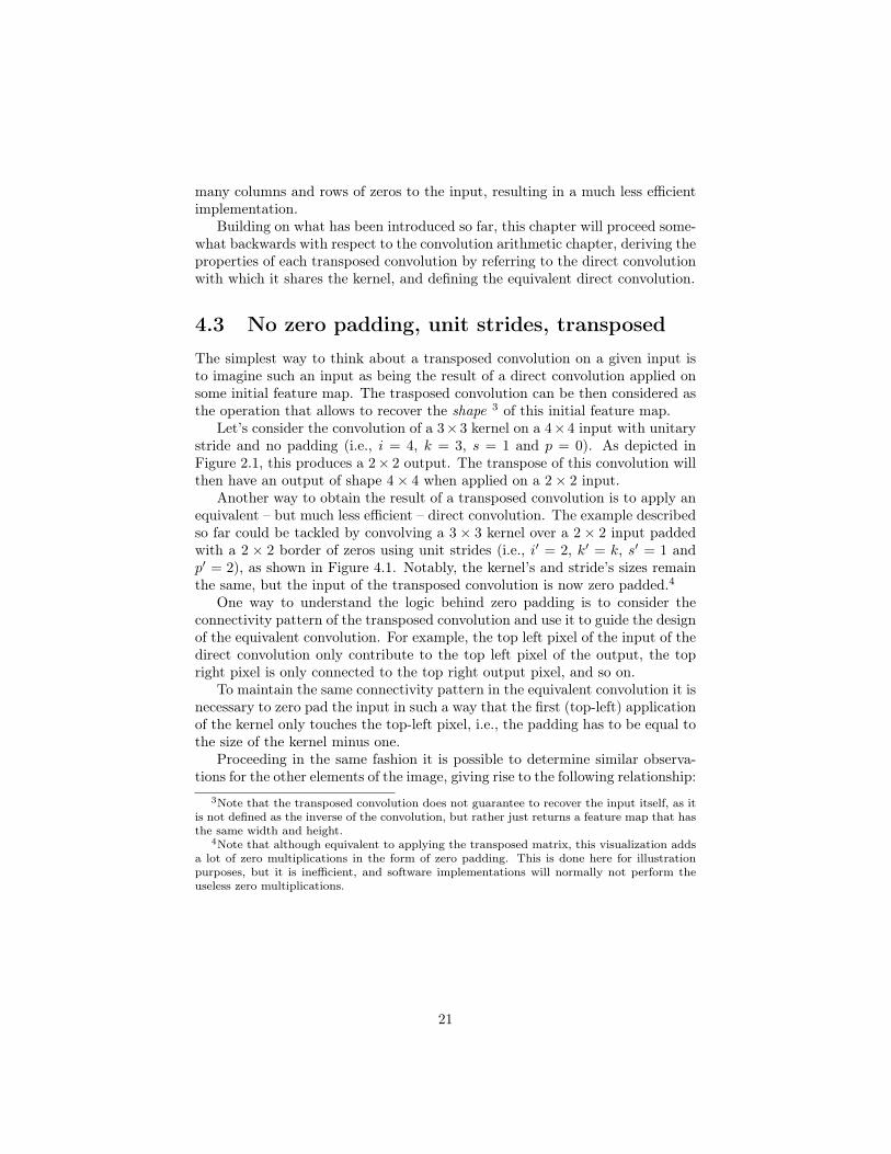
4.1 Convolution as a matrix operationTake for example the convolution represented in Figure 2.1. If the input andoutput were to be unrolled into vectors from left to right, top to bottom, theconvolution could be represented as a sparse matrix C where the non-zero ele-ments are the elements wi,j of the kernel (with i and j being the row and columnof the kernel respectively):
w0,0 w0,1 w0,2 0 w1,0 w1,1 w1,2 0 w2,0 w2,1 w2,2 0 0 0 0 00 w0,0 w0,1 w0,2 0 w1,0 w1,1 w1,2 0 w2,0 w2,1 w2,2 0 0 0 00 0 0 0 w0,0 w0,1 w0,2 0 w1,0 w1,1 w1,2 0 w2,0 w2,1 w2,2 00 0 0 0 0 w0,0 w0,1 w0,2 0 w1,0 w1,1 w1,2 0 w2,0 w2,1 w2,2
This linear operation takes the input matrix flattened as a 16-dimensional
vector and produces a 4-dimensional vector that is later reshaped as the 2 × 2output matrix.
Using this representation, the backward pass is easily obtained by trans-posing C; in other words, the error is backpropagated by multiplying the losswith CT . This operation takes a 4-dimensional vector as input and producesa 16-dimensional vector as output, and its connectivity pattern is compatiblewith C by construction.
Notably, the kernel w defines both the matrices C and CT used for theforward and backward passes.
4.2 Transposed convolutionLet’s now consider what would be required to go the other way around, i.e.,map from a 4-dimensional space to a 16-dimensional space, while keeping theconnectivity pattern of the convolution depicted in Figure 2.1. This operationis known as a transposed convolution.
Transposed convolutions – also called fractionally strided convolutions ordeconvolutions1 – work by swapping the forward and backward passes of a con-volution. One way to put it is to note that the kernel defines a convolution, butwhether it’s a direct convolution or a transposed convolution is determined byhow the forward and backward passes are computed.
For instance, although the kernel w defines a convolution whose forward andbackward passes are computed by multiplying with C and CT respectively, italso defines a transposed convolution whose forward and backward passes arecomputed by multiplying with CT and (CT )T = C respectively.2
Finally note that it is always possible to emulate a transposed convolutionwith a direct convolution. The disadvantage is that it usually involves adding
1The term “deconvolution” is sometimes used in the literature, but we advocate against iton the grounds that a deconvolution is mathematically defined as the inverse of a convolution,which is different from a transposed convolution.
2The transposed convolution operation can be thought of as the gradient of some convolu-tion with respect to its input, which is usually how transposed convolutions are implementedin practice.
20
many columns and rows of zeros to the input, resulting in a much less efficientimplementation.
Building on what has been introduced so far, this chapter will proceed some-what backwards with respect to the convolution arithmetic chapter, deriving theproperties of each transposed convolution by referring to the direct convolutionwith which it shares the kernel, and defining the equivalent direct convolution.
4.3 No zero padding, unit strides, transposedThe simplest way to think about a transposed convolution on a given input isto imagine such an input as being the result of a direct convolution applied onsome initial feature map. The trasposed convolution can be then considered asthe operation that allows to recover the shape 3 of this initial feature map.
Let’s consider the convolution of a 3×3 kernel on a 4×4 input with unitarystride and no padding (i.e., i = 4, k = 3, s = 1 and p = 0). As depicted inFigure 2.1, this produces a 2× 2 output. The transpose of this convolution willthen have an output of shape 4× 4 when applied on a 2× 2 input.
Another way to obtain the result of a transposed convolution is to apply anequivalent – but much less efficient – direct convolution. The example describedso far could be tackled by convolving a 3× 3 kernel over a 2× 2 input paddedwith a 2 × 2 border of zeros using unit strides (i.e., i′ = 2, k′ = k, s′ = 1 andp′ = 2), as shown in Figure 4.1. Notably, the kernel’s and stride’s sizes remainthe same, but the input of the transposed convolution is now zero padded.4
One way to understand the logic behind zero padding is to consider theconnectivity pattern of the transposed convolution and use it to guide the designof the equivalent convolution. For example, the top left pixel of the input of thedirect convolution only contribute to the top left pixel of the output, the topright pixel is only connected to the top right output pixel, and so on.
To maintain the same connectivity pattern in the equivalent convolution it isnecessary to zero pad the input in such a way that the first (top-left) applicationof the kernel only touches the top-left pixel, i.e., the padding has to be equal tothe size of the kernel minus one.
Proceeding in the same fashion it is possible to determine similar observa-tions for the other elements of the image, giving rise to the following relationship:
3Note that the transposed convolution does not guarantee to recover the input itself, as itis not defined as the inverse of the convolution, but rather just returns a feature map that hasthe same width and height.
4Note that although equivalent to applying the transposed matrix, this visualization addsa lot of zero multiplications in the form of zero padding. This is done here for illustrationpurposes, but it is inefficient, and software implementations will normally not perform theuseless zero multiplications.
21
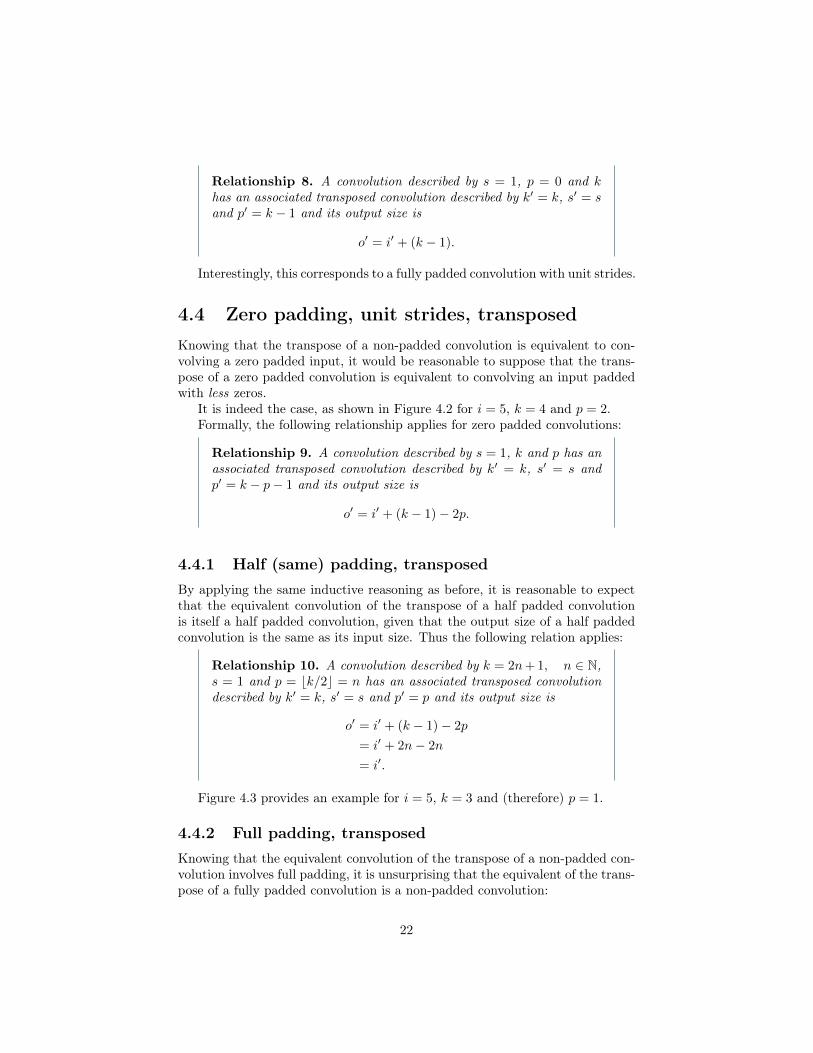
Relationship 8. A convolution described by s = 1, p = 0 and khas an associated transposed convolution described by k′ = k, s′ = sand p′ = k − 1 and its output size is
o′ = i′ + (k − 1).
Interestingly, this corresponds to a fully padded convolution with unit strides.
4.4 Zero padding, unit strides, transposedKnowing that the transpose of a non-padded convolution is equivalent to con-volving a zero padded input, it would be reasonable to suppose that the trans-pose of a zero padded convolution is equivalent to convolving an input paddedwith less zeros.
It is indeed the case, as shown in Figure 4.2 for i = 5, k = 4 and p = 2.Formally, the following relationship applies for zero padded convolutions:
Relationship 9. A convolution described by s = 1, k and p has anassociated transposed convolution described by k′ = k, s′ = s andp′ = k − p− 1 and its output size is
o′ = i′ + (k − 1)− 2p.
4.4.1 Half (same) padding, transposedBy applying the same inductive reasoning as before, it is reasonable to expectthat the equivalent convolution of the transpose of a half padded convolutionis itself a half padded convolution, given that the output size of a half paddedconvolution is the same as its input size. Thus the following relation applies:
Relationship 10. A convolution described by k = 2n+1, n ∈ N,s = 1 and p = bk/2c = n has an associated transposed convolutiondescribed by k′ = k, s′ = s and p′ = p and its output size is
o′ = i′ + (k − 1)− 2p
= i′ + 2n− 2n
= i′.
Figure 4.3 provides an example for i = 5, k = 3 and (therefore) p = 1.
4.4.2 Full padding, transposedKnowing that the equivalent convolution of the transpose of a non-padded con-volution involves full padding, it is unsurprising that the equivalent of the trans-pose of a fully padded convolution is a non-padded convolution:
22

Figure 4.1: The transpose of convolving a 3× 3 kernel over a 4× 4 input usingunit strides (i.e., i = 4, k = 3, s = 1 and p = 0). It is equivalent to convolvinga 3× 3 kernel over a 2× 2 input padded with a 2× 2 border of zeros using unitstrides (i.e., i′ = 2, k′ = k, s′ = 1 and p′ = 2).
Figure 4.2: The transpose of convolving a 4×4 kernel over a 5×5 input paddedwith a 2 × 2 border of zeros using unit strides (i.e., i = 5, k = 4, s = 1 andp = 2). It is equivalent to convolving a 4 × 4 kernel over a 6 × 6 input paddedwith a 1 × 1 border of zeros using unit strides (i.e., i′ = 6, k′ = k, s′ = 1 andp′ = 1).
Figure 4.3: The transpose of convolving a 3× 3 kernel over a 5× 5 input usinghalf padding and unit strides (i.e., i = 5, k = 3, s = 1 and p = 1). It isequivalent to convolving a 3 × 3 kernel over a 5 × 5 input using half paddingand unit strides (i.e., i′ = 5, k′ = k, s′ = 1 and p′ = 1).
23

Relationship 11. A convolution described by s = 1, k and p = k−1has an associated transposed convolution described by k′ = k, s′ = sand p′ = 0 and its output size is
o′ = i′ + (k − 1)− 2p
= i′ − (k − 1)
Figure 4.4 provides an example for i = 5, k = 3 and (therefore) p = 2.
4.5 No zero padding, non-unit strides, transposedUsing the same kind of inductive logic as for zero padded convolutions, onemight expect that the transpose of a convolution with s > 1 involves an equiv-alent convolution with s < 1. As will be explained, this is a valid intuition,which is why transposed convolutions are sometimes called fractionally stridedconvolutions.
Figure 4.5 provides an example for i = 5, k = 3 and s = 2 which helpsunderstand what fractional strides involve: zeros are inserted between inputunits, which makes the kernel move around at a slower pace than with unitstrides.5
For the moment, it will be assumed that the convolution is non-padded(p = 0) and that its input size i is such that i − k is a multiple of s. In thatcase, the following relationship holds:
Relationship 12. A convolution described by p = 0, k and s andwhose input size is such that i−k is a multiple of s, has an associatedtransposed convolution described by i′, k′ = k, s′ = 1 and p′ = k−1,where i′ is the size of the stretched input obtained by adding s − 1zeros between each input unit, and its output size is
o′ = s(i′ − 1) + k.
4.6 Zero padding, non-unit strides, transposedWhen the convolution’s input size i is such that i + 2p − k is a multiple of s,the analysis can extended to the zero padded case by combining Relationship 9and Relationship 12:
5Doing so is inefficient and real-world implementations avoid useless multiplications byzero, but conceptually it is how the transpose of a strided convolution can be thought of.
24
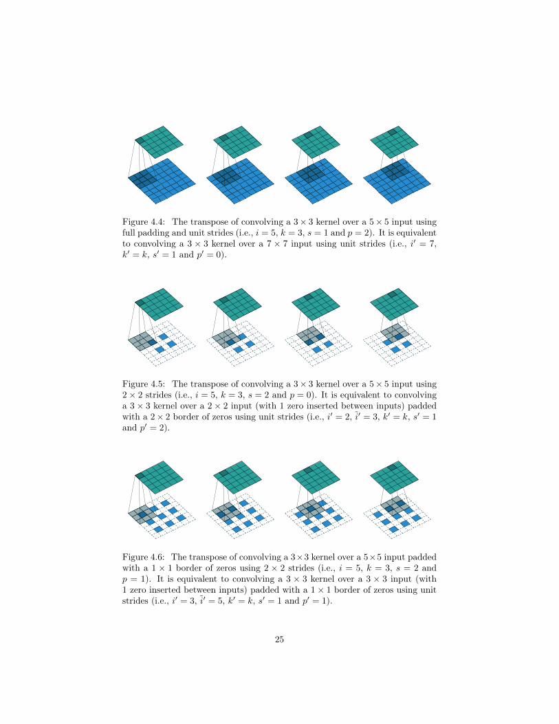
Figure 4.4: The transpose of convolving a 3× 3 kernel over a 5× 5 input usingfull padding and unit strides (i.e., i = 5, k = 3, s = 1 and p = 2). It is equivalentto convolving a 3 × 3 kernel over a 7 × 7 input using unit strides (i.e., i′ = 7,k′ = k, s′ = 1 and p′ = 0).
Figure 4.5: The transpose of convolving a 3× 3 kernel over a 5× 5 input using2× 2 strides (i.e., i = 5, k = 3, s = 2 and p = 0). It is equivalent to convolvinga 3× 3 kernel over a 2× 2 input (with 1 zero inserted between inputs) paddedwith a 2× 2 border of zeros using unit strides (i.e., i′ = 2, i′ = 3, k′ = k, s′ = 1and p′ = 2).
Figure 4.6: The transpose of convolving a 3×3 kernel over a 5×5 input paddedwith a 1 × 1 border of zeros using 2 × 2 strides (i.e., i = 5, k = 3, s = 2 andp = 1). It is equivalent to convolving a 3 × 3 kernel over a 3 × 3 input (with1 zero inserted between inputs) padded with a 1× 1 border of zeros using unitstrides (i.e., i′ = 3, i′ = 5, k′ = k, s′ = 1 and p′ = 1).
25

Relationship 13. A convolution described by k, s and p and whoseinput size i is such that i+2p−k is a multiple of s has an associatedtransposed convolution described by i′, k′ = k, s′ = 1 and p′ =k − p − 1, where i′ is the size of the stretched input obtained byadding s− 1 zeros between each input unit, and its output size is
o′ = s(i′ − 1) + k − 2p.
Figure 4.6 provides an example for i = 5, k = 3, s = 2 and p = 1.The constraint on the size of the input i can be relaxed by introducing
another parameter a ∈ {0, . . . , s − 1} that allows to distinguish between the sdifferent cases that all lead to the same i′:
Relationship 14. A convolution described by k, s and p has anassociated transposed convolution described by a, i′, k′ = k, s′ = 1and p′ = k−p−1, where i′ is the size of the stretched input obtainedby adding s− 1 zeros between each input unit, and a = (i+ 2p− k)mod s represents the number of zeros added to the bottom and rightedges of the input, and its output size is
o′ = s(i′ − 1) + a+ k − 2p.
Figure 4.7 provides an example for i = 6, k = 3, s = 2 and p = 1.
26

Figure 4.7: The transpose of convolving a 3×3 kernel over a 6×6 input paddedwith a 1 × 1 border of zeros using 2 × 2 strides (i.e., i = 6, k = 3, s = 2 andp = 1). It is equivalent to convolving a 3 × 3 kernel over a 2 × 2 input (with1 zero inserted between inputs) padded with a 1 × 1 border of zeros (with anadditional border of size 1 added to the bottom and right edges) using unitstrides (i.e., i′ = 3, i′ = 5, a = 1, k′ = k, s′ = 1 and p′ = 1).
27
Chapter 5
Miscellaneous convolutions
5.1 Dilated convolutionsReaders familiar with the deep learning literature may have noticed the term“dilated convolutions” (or “atrous convolutions”, from the French expression con-volutions à trous) appear in recent papers. Here we attempt to provide an in-tuitive understanding of dilated convolutions. For a more in-depth descriptionand to understand in what contexts they are applied, see Chen et al. (2014); Yuand Koltun (2015).
Dilated convolutions “inflate” the kernel by inserting spaces between the ker-nel elements. The dilation “rate” is controlled by an additional hyperparameterd. Implementations may vary, but there are usually d−1 spaces inserted betweenkernel elements such that d = 1 corresponds to a regular convolution.
Dilated convolutions are used to cheaply increase the receptive field of outputunits without increasing the kernel size, which is especially effective when multi-ple dilated convolutions are stacked one after another. For a concrete example,see Oord et al. (2016), in which the proposed WaveNet model implements anautoregressive generative model for raw audio which uses dilated convolutionsto condition new audio frames on a large context of past audio frames.
To understand the relationship tying the dilation rate d and the output sizeo, it is useful to think of the impact of d on the effective kernel size. A kernelof size k dilated by a factor d has an effective size
k = k + (k − 1)(d− 1).
This can be combined with Relationship 6 to form the following relationship fordilated convolutions:
Relationship 15. For any i, k, p and s, and for a dilation rate d,
o =
⌊i+ 2p− k − (k − 1)(d− 1)
s
⌋+ 1.
28
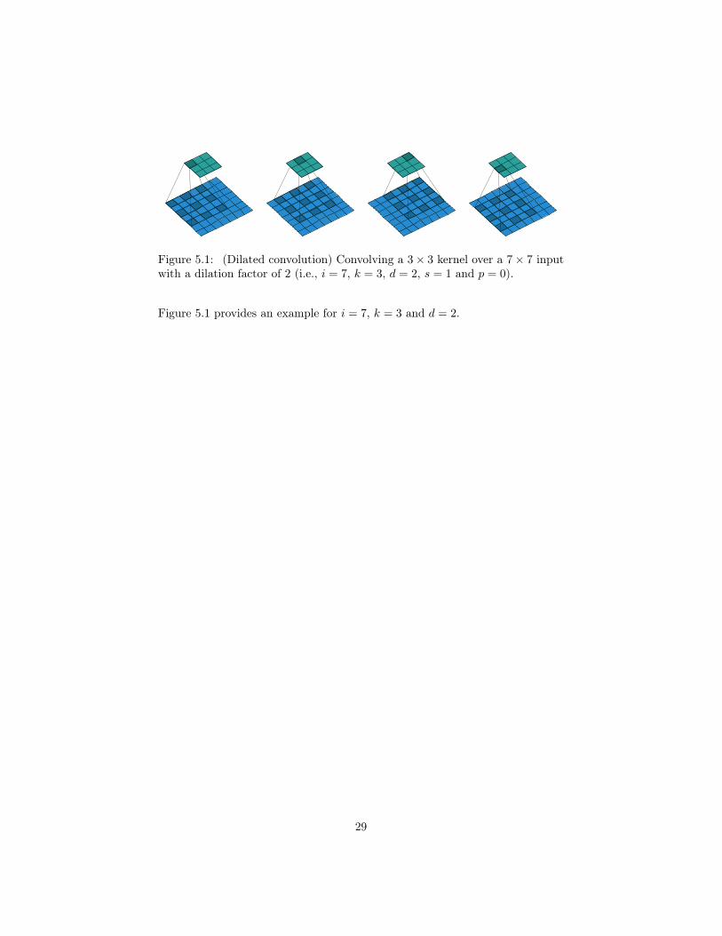
Figure 5.1: (Dilated convolution) Convolving a 3× 3 kernel over a 7× 7 inputwith a dilation factor of 2 (i.e., i = 7, k = 3, d = 2, s = 1 and p = 0).
Figure 5.1 provides an example for i = 7, k = 3 and d = 2.
29
Bibliography
Abadi, M., Agarwal, A., Barham, P., Brevdo, E., Chen, Z., Citro, C., Corrado,G. S., Davis, A., Dean, J., Devin, M., et al. (2015). Tensorflow: Large-scale machine learning on heterogeneous systems. Software available fromtensorflow.org .
Bastien, F., Lamblin, P., Pascanu, R., Bergstra, J., Goodfellow, I., Bergeron,A., Bouchard, N., Warde-Farley, D., and Bengio, Y. (2012). Theano: newfeatures and speed improvements. arXiv preprint arXiv:1211.5590 .
Bergstra, J., Breuleux, O., Bastien, F., Lamblin, P., Pascanu, R., Desjardins,G., Turian, J., Warde-Farley, D., and Bengio, Y. (2010). Theano: A cpu andgpu math compiler in python. In Proc. 9th Python in Science Conf , pages1–7.
Boureau, Y., Bach, F., LeCun, Y., and Ponce, J. (2010a). Learning mid-levelfeatures for recognition. In Proc. International Conference on Computer Vi-sion and Pattern Recognition (CVPR’10). IEEE.
Boureau, Y., Ponce, J., and LeCun, Y. (2010b). A theoretical analysis of featurepooling in vision algorithms. In Proc. International Conference on Machinelearning (ICML’10).
Boureau, Y., Le Roux, N., Bach, F., Ponce, J., and LeCun, Y. (2011). Ask thelocals: multi-way local pooling for image recognition. In Proc. InternationalConference on Computer Vision (ICCV’11). IEEE.
Chen, L.-C., Papandreou, G., Kokkinos, I., Murphy, K., and Yuille, A. L. (2014).Semantic image segmentation with deep convolutional nets and fully con-nected crfs. arXiv preprint arXiv:1412.7062 .
Collobert, R., Kavukcuoglu, K., and Farabet, C. (2011). Torch7: A matlab-likeenvironment for machine learning. In BigLearn, NIPS Workshop, numberEPFL-CONF-192376.
Goodfellow, I., Bengio, Y., and Courville, A. (2016). Deep learning. Book inpreparation for MIT Press.
30
Im, D. J., Kim, C. D., Jiang, H., and Memisevic, R. (2016). Generating imageswith recurrent adversarial networks. arXiv preprint arXiv:1602.05110 .
Jia, Y., Shelhamer, E., Donahue, J., Karayev, S., Long, J., Girshick, R., Guadar-rama, S., and Darrell, T. (2014). Caffe: Convolutional architecture for fastfeature embedding. In Proceedings of the ACM International Conference onMultimedia, pages 675–678. ACM.
Krizhevsky, A., Sutskever, I., and Hinton, G. E. (2012). Imagenet classificationwith deep convolutional neural networks. In Advances in neural informationprocessing systems, pages 1097–1105.
Le Cun, Y., Bottou, L., and Bengio, Y. (1997). Reading checks with multilayergraph transformer networks. In Acoustics, Speech, and Signal Processing,1997. ICASSP-97., 1997 IEEE International Conference on, volume 1, pages151–154. IEEE.
Long, J., Shelhamer, E., and Darrell, T. (2015). Fully convolutional networks forsemantic segmentation. In Proceedings of the IEEE Conference on ComputerVision and Pattern Recognition, pages 3431–3440.
Oord, A. v. d., Dieleman, S., Zen, H., Simonyan, K., Vinyals, O., Graves, A.,Kalchbrenner, N., Senior, A., and Kavukcuoglu, K. (2016). Wavenet: Agenerative model for raw audio. arXiv preprint arXiv:1609.03499 .
Radford, A., Metz, L., and Chintala, S. (2015). Unsupervised representa-tion learning with deep convolutional generative adversarial networks. arXivpreprint arXiv:1511.06434 .
Saxe, A., Koh, P. W., Chen, Z., Bhand, M., Suresh, B., and Ng, A. (2011).On random weights and unsupervised feature learning. In L. Getoor andT. Scheffer, editors, Proceedings of the 28th International Conference on Ma-chine Learning (ICML-11), ICML ’11, pages 1089–1096, New York, NY, USA.ACM.
Visin, F., Kastner, K., Courville, A. C., Bengio, Y., Matteucci, M., and Cho,K. (2015). Reseg: A recurrent neural network for object segmentation.
Yu, F. and Koltun, V. (2015). Multi-scale context aggregation by dilated con-volutions. arXiv preprint arXiv:1511.07122 .
Zeiler, M. D. and Fergus, R. (2014). Visualizing and understanding convolu-tional networks. In Computer vision–ECCV 2014 , pages 818–833. Springer.
Zeiler, M. D., Taylor, G. W., and Fergus, R. (2011). Adaptive deconvolutionalnetworks for mid and high level feature learning. In Computer Vision (ICCV),2011 IEEE International Conference on, pages 2018–2025. IEEE.
31