WORKING PAPER F-2009-03

Lasse Bork

Estimating US Monetary Policy Shocks Using a Factor-Augmented Vector Autoregression: An EM Algorithm Approach

Finance Research Group

Estimating US Monetary Policy Shocks Using a

Factor-Augmented Vector Autoregression: An

EM Algorithm Approach�

Lasse Borky

Current Version: February, 2009First Draft: July 30, 2008

Abstract

Economy-wide e¤ects of shocks to the US federal funds rate are esti-mated in a state space model with 120 US macroeconomic and �nancialtime series driven by the dynamics of the federal funds rate and a few dy-namic factors. This state space system is denoted a factor-augmented VAR(FAVAR) by Bernanke et al. (2005). I estimate the FAVAR by the fullyparametric one-step EM algorithm as an alternative to the two-step prin-cipal component method and the one-step Bayesian method in Bernankeet al. (2005). The EM algorithm which is an iterative maximum likelihoodmethod estimates all the parameters and the dynamic factors simultane-ously and allows for classical inference. I demonstrate empirically that thesame impulse responses but better �t emerge robustly from a low orderFAVAR with eight correlated factors compared to a high order FAVARwith fewer correlated factors, for instance four factors. This empirical re-sult accords with one of the theoretical results from Bai & Ng (2007) inwhich it is shown that the information in complicated factor dynamics maybe substituted by panel information.

JEL classi�cations: E3, E43, E51, E52, C33.Keywords: Monetary policy, large cross-sections, factor-augmented vec-tor autoregression, EM algorithm, state space.

�I thank Tom Engsted for helpful comments. Any remaining errors are my own.yFinance Research Group, Department of Business Studies, Aarhus School of Business, Uni-

versity of Aarhus, Fuglesangs Allé 4, DK-8210 Aarhus V, Denmark. A¢ liated with CREATESat the University of Aarhus, a research center funded by the Danish National Research Foun-dation. Email: lbo@lassebork.dk.

1

1 Introduction

This paper estimates the "economy-wide" response to shocks to the US federal

funds rate using an iterative maximum likelihood estimation method. The data

description of the US economy is con�ned to a large cross-section of 120 macro-

economic and �nancial time series and the comovement of these time series over

time is shown to be adequately described in terms of a few dynamic latent driving

forces (dynamic factors) and the US federal funds rate. Technically, the 120 time

series constitute the measured part in a state space system. The state transition

part of this system contains the dynamics of the driving forces and is represented

as a vector autoregression of the federal funds rate augmented by a few dynamic

factors extracted from the large cross-section of time series. The complete state

space system in turn allows for an empirical study of the response of each of the

120 observed variables following a shock to the federal funds rate.

This setup is what Bernanke et al. (2005) denote a factor-augmented vec-

tor autoregressive (FAVAR) approach and this paper is closely related to both

their approach and the data used. While Bernanke et al. (2005) estimate their

FAVAR using both a two-step semi-parametric principal component method and

a one-step Bayesian likelihood method, this paper contributes to the literature by

estimating the FAVAR by a one-step fully parametric iterative maximum likeli-

hood method, the Expectation Maximization (EM) algorithm. In fact, several of

the future research issues that Bernanke et al. (2005) address in their conclusion

are cited below and discussed in this paper:

"Future work should investigate more fully the properties of FAVARs, alter-

native estimation methods and alternative identi�cation schemes. In particular,

further comparison of the estimation methods based on principal components and

on Gibbs sampling is likely to be worthwhile. Another interesting direction is to

try to interpret the estimated factors more explicitly". Bernanke et al. (2005)

page 415, §3.

Speci�cally, the issue of alternative estimation methods is adressed by the

above-mentioned EM algorithm and the issue of alternative identi�cation schemes

is addressed by allowing for correlated dynamic factors in contrast to the typical

application of uncorrelated dynamic factors1. Finally, a thorough investigation

1The issue of interpretation of the estimated factors is addressed in Bork et al. (2008) in

2

of the properties of the FAVARs is undertaken by estimating a large number of

econometric speci�cations of FAVARs and subsequently evaluating these in terms

of statistical �t, speci�cation tests and implications for monetary policy analysis.

Consider each of these three contributions in turn.

Similar to the one-step Bayesian method, the EM algorithm estimates all the

parameters and the dynamic factors simultaneously in contrast to the two-step

principal component method. The last-mentioned method extracts the factors

non-parametrically from the data without imposing any dynamic properties on

the factors in the �rst step. The second step estimates the dynamic properties

of the factors through a vector autoregression treating the factors as observed2.

One complication in the principal component method is how to separate the

observed federal funds rate from the latent factors in the extraction of these

factors, which in contrast is handled in a straightforward manner in the one-

step method. However, the advantage of the principal component method is its

computational simplicity. Finally, the fully parametric likelihood approach of the

EM algorithm allows for classical inference.

The alternative identi�cation scheme allows the factors to be correlated which

is relevant if macroeconomic interpretation is to be attached to these latent fac-

tors. For instance, if the �rst factor is interpreted as an industrial production

factor and the second is interpreted as an unemployment factor, then we would

expect these factors to be negatively correlated. The correlated factor approach

in this paper allows for this feature.

Finally, the robustness of the preferred econometric model is evaluated against

several model speci�cations in terms of the number of factors included in the

FAVAR and the number of lags of these factors using various information criteria.

Speci�cally, careful model selection leads to a preferred model characterized by

eight factors with a particular parsimonious factor dynamics. This model yields

an eleven percentage point better �t of the panel and reaches the same conclusions

from the empirical monetary policy analysis as the benchmark model with four

factors but a complicated VAR(13) factor dynamics. This �nding accords with

which the EM algorithm is also applied.2The di¤erence between the estimated factors and the true factors vanishes as the cross-

section dimension and the time series dimension approach in�nity, cf. Bai & Ng (2002).

3

one of the theoretical results from Bai & Ng (2007) in which it is shown that

complicated factor dynamics may be substituted by panel information (in terms

of more factors). The eight correlated factors are found to be closely related

to observed variables; for instance, the �rst and most important latent factor is

interpreted as an industrial production factor, the second as an unemployment

factor, the third as a NAPM3 factor, and so on.

Factor models have a long tradition in applied economics, �nance and other

sciences and hence only a few observations may be needed to motivate why we

should continue to be interested in variants of factor models.

Firstly, factor models enable a reduction in the number of explanatory vari-

ables (factors) when the variation of a cross-section of variables can be decom-

posed into a low-dimensional common component re�ecting the common sources

of variation and a variable speci�c idiosyncratic component; cf. Ross (1976),

Chamberlain (1983), Chamberlain & Rothschild (1983) and Geweke & Zhou

(1996) for cross-section applications within �nance. Macroeconomic variables

tend to comove over the business cycle and therefore their common variation

over time may be explained by a few dynamic factor(s); cf. Geweke (1977),

Sargent & Sims (1977) and Geweke & Singleton (1981) for the �rst generation

of the dynamic factor (index) models estimated by spectral density maximum

likelihood methods. Engle & Watson (1981) propose a time domain maximum

likelihood method and Watson & Engle (1983) and Quah & Sargent (1993) apply

the Expectation Maximization (EM) algorithm introduced by Dempster et al.

(1977).

Secondly, large cross-sections of time series are nowadays available to re-

searchers and policy makers, including central bankers that "follow literally hun-

dreds of data series", as expressed by Bernanke et al. (2005). The potential gains

of using large information sets are more precise forecasts and a better under-

standing of the dynamics of the economy. In the context of the FAVAR, a much

richer information set is utilized in the econometric model than in the standard

vector autoregressive (VAR) model, leaving less scope for the omitted variable

problem. Moreover, because macroeconomic data are prone to measurement er-

rors4, dynamic factor analysis of large panels may help to �lter out the observed

3Related to surveys by National Association of Purchasing Management.4Sargent (1989) shows how the existence of measurement error leads to a dynamic factor

4

counterpart of a theoretical variable, like "in�ation", which may not be well rep-

resented by a single observed time series.

Recently, a considerable amount of research has been devoted to the econo-

metric theory and empirical analysis of large dimensional approximate5 dynamic

factor models, notably the generalized dynamic factor model by Forni et al. (2000,

2004, 2005) and the static representation of the dynamic factor model by Stock

& Watson (2002a,b). Both approaches allow for a general error structure and

facilitate dynamic factor analysis of large panels through a few dynamic factors

that are extracted from the panel X using non-parametric dynamic and static

principal component methods, respectively6. A vector autoregression of the fac-

tors may be considered as a second step treating the factors as observed if one is

interested in structural VAR analysis; see for instance Stock & Watson (2005).

Note at this stage that in the FAVAR of Bernanke et al. (2005), the common

variation of the panel dataset is not limited to being explained by a set of latent

dynamic factors, as in the Stock &Watson model, but also observed variables (the

federal funds rate) may enter into this set and accordingly interact dynamically

with the factors.

Econometric theory of the determination of the number of factors has recently

been developed, notably by Hallin & Liska (2007), Stock & Watson (2005) and

Bai & Ng (2007) for the Forni, Hallin, Lippi & Reichlin class of models and by Bai

& Ng (2002) for the class of dynamic factor models in the static representation.

Including more factors in the factor model increases the statistical �t of the panel

but at the cost of parsimony, whereas choosing too few factors means that the

factor space is not su¢ ciently spanned by the estimated factors. The papers

propose various information criteria to guide us in the selection of the number

of factors but they do not provide information about the number of lags in the

index model.5In the �rst generation exact factor models like Ross (1976) or Geweke (1977), Sargent &

Sims (1977) and Geweke & Singleton (1981), the idiosyncratic components are orthogonal. How-ever, the approximate factor models allow for some "local" correlation among the idiosyncraticcomponents.

6Stock & Watson (2002a) show that the space spanned by the true number of factors, F;can be consistently estimated by the non-parametric principal component method when thecross-section dimension (N) and the time dimension (T ) of the panel are large and the numberof principal components is at least as large as the true number of factors.

5

VAR. Consequently, the model selection problem in this paper is solved using the

above-mentioned information criteria, and for a given number of factors, also the

standard Akaike and Schwartz information criteria.

Since the initial work of Forni, Hallin, Lippi & Reichlin and Stock & Wat-

son, dynamic factor models have been used in an increasing number of applica-

tions7 starting with the construction of coincident indicator indices as in Forni

et al. (2001), forecasting where dynamic factors enter the forecasting equation,

cf. Stock &Watson (2002a,b, 2006), and very recently nowcasting as in Giannone

et al. (2008) where dynamic factor analysis of large panels is used to assess the

current-quarter economic conditions. The use of dynamic factors in �nancial asset

pricing applications includes the estimation of the conditional risk-return rela-

tion in Ludvigson & Ng (2007) and bond market applications by Mönch (2008)

and Ludvigson & Ng (2008). Finally, a number of papers to which this paper is

particularly related adopt the factor approach for monetary policy analyses with

at least two advantages over the traditional VAR.

Firstly, the curse of dimensionality in the VAR is turned into a "blessing"

of dimensionality in the factor models as expressed by Stock & Watson (2006)

which is particularly useful for representing the data-rich environment in which

central banks and professional forecasters actually operate.

Secondly, to assess the current and expected future state of the economy in

policy decision making, the central banks are faced with a variety of data in

di¤erent frequencies, with missing observations and in a preliminary or revised

form. Therefore, it can be argued that empirical policy analysis researchers should

look at the real-time data that the central bank had at its disposal instead of the

revised data and this can be achieved by the dynamic factor model, cf. the

approach by Giannone et al. (2008).

Giannone et al. (2004) perform a real-time monetary policy study and �nd

that the US economy is driven by two stochastic shocks (real and nominal) which

implies that the federal funds rate should mainly track these two shocks, they

argue. Bernanke & Boivin (2003) also consider a real-time dataset in addition

to a larger cross-section of revised time series. They �nd that the scope of the

dataset (the number of variables in the cross-section, N) is more important for

7A detailed account of empirical applications can be found in Reichlin (2003) and Breitung& Eickmeier (2006).

6

the forecasting performance of expected in�ation and real activity in the forward-

looking Taylor rule than the real-time feature. In a similar setup, Favero et al.

(2005) study a revised cross-section of US and Euro area data. Common for these

studies is the estimation of the factors by principal component methods which

are then included in a low-order VAR in the second step to allow for impulse

response analysis of monetary policy shocks and these responses are found to

be more in line with the predictions from theory. However, a critical step in

the empirical monetary policy analysis is a proper disentanglement of the federal

funds rate from the estimated factors and the paper by Bernanke et al. (2005) is

particularly clear about this identi�cation issue.

As an alternative to the two-step principal component estimation method,

one-step Bayesian estimation techniques are applied in Bernanke et al. (2005)

as well as in Banbura et al. (2008). The former choose thirteen lags in their

FAVAR speci�cation while the latter also estimate this variant in addition to

lag speci�cations determined by the BIC criterion. The fully parametric one-step

EM algorithm method has recently been applied to large panels in Jungbacker

& Koopman (2008) that estimate a dynamic factor model with a VAR(1) in the

orthogonal factors and in Reis & Watson (2008) that estimate pure in�ation with

a VAR(4) in absolute-price and relative-price components.

Based on this selective literature overview there seems to be a need for explor-

ing the consequences of model selection for not only policy evaluation but also

in terms of statistical signi�cance of parameters and statistical �t of the various

components in the economy such as in�ation, employment, production etc. This

issue is taken up in this paper and consequently several model speci�cations rang-

ing from a few correlated factors with only one lag to many correlated factors with

rich factor dynamics are estimated in an EM algorithm setup. I show how identi-

fying restrictions can easily be imposed on the parameters including restrictions

on the VAR parameters, if needed. This is in contrast to the Bayesian approach

where these kind of restrictions seemingly lead to excessive computational cost,

cf. Bernanke et al. (2005).

Furthermore, though the EM algorithm �nds the vicinity of the maximum

quickly, the convergence to the maximum is almost excruciatingly slow (linear

convergence rate) and consequently hybrid methods combining the EM algorithm

and the BFGS have been proposed in the literature. Therefore, I also apply the

7

hybrid EM-BFGS as described by Jungbacker & Koopman (2008) in order to

speed up the convergence.

The rest of the paper is organized as follows. The factor-augmented VAR

is presented in section 2 while identi�cation issues and the estimation method

are presented in section 3. Section 4 details the empirical results and section 5

concludes. The appendices contain details on the Kalman �lter and smoother as

well as the EM algorithm.

2 Model framework: The factor-augmented VAR

Two ingredients need to be combined to set up the FAVAR. The �rst ingredient

is the dynamic factor model and the second ingredient is the standard VAR with

observed variables. Before mixing the ingredients, one thing is important to

note: the federal funds rate (FFR) is both part of the observed variables in the

panel (the measured part of the state space system) and also part of the state

variables (the state transition equation in the state space system) which include

the dynamic latent factors. Therefore, to allow for this feature the standard

dynamic factor model is modi�ed and this is described in detail below.

This section will center around the static representation of the dynamic fac-

tor model in state space form which can be seen as a special case of the large

dimensional generalized dynamic factor model; see Bai & Ng (2007) for a clear

exposition. Following the presentation of the dynamic factor model, the FFR is

properly identi�ed in the panel and then added to the state transition variables.

This may sound like a backward description of the factor-augmented VAR but

nevertheless I �nd this the most intuitive route towards the FAVAR.

The key implication of the dynamic factor model is that the variation of each of

the N observed variables in the panel X can be decomposed into two orthogonal

components, that is a component � common to all variables and an idiosyncratic

component � speci�c to each variable. The common component is driven by a few

common factors and this component accounts for the covariation of the observed

variables at all lags and leads. Consequently, the ith variable in the panel X8 at

8All variables in the panel are transformed into stationary variables with mean zero and unitvariance. See section 4.1.

8

time t can be written as:

xit = �it + �it (1)

for i = 1; ::; N and t = 1; ::; T with E��it�js

�= 0 8 i; j; t; s but with a potentially

limited amount of correlation among the idiosyncratic components in the new

generation of dynamic factor models. The following description encompasses

the dynamic factor model which is characterized by the dynamic loading on the

common factors as well as the static representation of the dynamic factor model

characterized by the static loadings. The distinguishing features of the models

will become useful in later discussions.

Consider as in Forni et al. (2005), the speci�cation of the N � 1 vector ofthe common component at time t to be dynamically explained by the q common

factors ft such that �t = � (L) ft; where � (L) is a N � q matrix polynomial

in the lag-operator L of �nite order s9. To facilitate an interpretation of the

panel being driven entirely by q primitive iid shocks, the common component is

sometimes written as �t = � (L) "t, where � (L) represents the impulse-response

functions and accordingly for each variable records the responses in terms of

sign, magnitude and lag-structure following a shock to the underlying primitive

shocks, "t10: Inserting the speci�cation of the common component in (1) results

in a dynamic factor model driven by q dynamic factors:

xit = �>i (L) ft + �it (2)

where �i (L) = �i;0+�i;1L+ � � �+�i;sLs: Stacking contemporaneous and s laggedvalues of ft in the q (s+ 1) dimensional vector Ft and the matching values of �i in

q (s+ 1) dimensional vector �i results in the static representation of the dynamic

9In�nite order of the lag-polynomiums is considered in the generalized dynamic factor modelof Forni et al. (2000).10Rewrite the factors in terms of the primitive shocks, ft = a (L) "t and as a result � (L) =

� (L) a (L) : See Forni et al. (2007) for a thorough discussion.

9

factor model in (2), which is driven by r = q (s+ 1) factors, Ft :

xit = �>i Ft + �it (3)

=

266664�i;0

�i;1...

�i;s

377775> 266664

ft

ft�1...

ft�s

377775+ �it

Notice how the dimension of Ft; r = q (s+ 1) depends on the heterogeneity

in the response of the data to the factors ft through � (L) or equivalently to the

primitive shocks "t through � (L).

Furthermore, Ft is governed by a dynamic process which depends on how

complicated the process governing ft is relative to the response heterogeneity of

the panel. Assuming that ft is an AR(h) process, Bai & Ng (2007)11 show that

Ft can be represented as a VAR(p) process with p = max (1; h� s) : Intuitively, if

the dynamic process of ft is particular simple then a VAR(1) should be su¢ cient.

Interestingly, a su¢ ciently heterogeneous dynamic response of the data may sub-

stitute for some otherwise complicated dynamics of ft; cf. the term (h� s) in

max (1; h� s) : I will refer to this result later in the discussion of the empirical

results.

The static representation of the dynamic factor model is now closed and can

be written in state space form:

Xt = �Ft + �t

Ft = �(L)Ft�1 +�"t(4)

where Xt = (x1;t; :::; xN;t)>, �t =

��1t;; :::; �N;t

�>is i.i.d N (0; R)12 and � =�

�>1 ; :::;�>N

�>is a N � r loading matrix. The state transition equation is sta-

tionary so that the pth order matrix polynomial � (L) has roots outside the unit

circle, � is a r� q matrix and "t is i.i.d N (0; Q). The unknowns in this Gaussian11They also discuss MA(h) and ARMA processes.12Note that the assumption of i.i.d idiosyncratic components in (4) de�nes an exact dynamic

factor model. This is certainly a strong assumption, particularly in the case of large panel datawhere local cross-sectional correlation within a group of similar variables should be expected.As such, equation (4) represents a misspeci�ed model. However, Doz et al. (2006) generate dataunder the assumption of an approximate factor model and show, for large N and T; that theexact factor model consistenly estimates the factors by a Gaussian (quasi)maximum likelihoodmethod. Speci�cally, they propose to use the EM algorithm.

10

state space model are the parameters in � = f�; R;� (L) ;�; Qg and the latentdynamic factors Ft:

The �nal step towards the FAVAR is the inclusion of the FFR in both Xt and

Ft (FFR is added to and ordered last in Ft). Speci�cally, the FFR in Xt loads

with unity on the last factor in Ft and zeros on the remaining latent factors,

such that the corresponding row in � for FFR is [0; :::; 0; 1]. In principle, an

idiosyncratic error could be attached to the FFR to capture the transition between

discretionary changes in the policy rate. In line with Bernanke et al. (2005), I

argue that the FFR is indeed measured without error whereas the other variables

may be measured with error. Applying these minor changes to the state space

form in (4) leads to the preferred FAVAR speci�cation. However, some identifying

restrictions need to be imposed on the econometric formulation to achieve distinct

factors, which, together with the estimation procedure is the topic of the following

section.

3 Identi�cation and estimation by the EM algo-

rithm

This section starts with a discussion of identi�cation schemes and then proceeds

to a brief description of the estimation procedure, that is the EM algorithm. I

also demonstrate how linear parameter restrictions can easily be imposed. Fi-

nally, a hybrid estimation method that combines the EM algorithm and the

Broyden-Fletcher-Goldfarb-Shanno (BFGS) method with analytical derivatives

is described.

The FAVAR model is highly over-parameterized as it stands in (4) and we

are not able to estimate a unique set of parameters, � with the data unless

identifying restrictions are imposed on�: This is a well-known problem of classical

factor analysis including the principal component approach to dynamic factor

analysis by Stock & Watson. Typically, these models are identi�ed by restricting

the covariance matrix of the factors to be an identity matrix, F>F=T = I but

sometimes also �>�=N = I is used. Neither of these identi�cation schemes is

su¢ cient in the one-step estimation of the state space model because the factors

are identi�ed by both the measurement equation and state transition equation

11

in (4) : Brie�y, for any orthogonal matrix P where PP> = I, it is possible to

construct an observationally equivalent model with ~� = �P�1 and ~F = PF that

still satis�es the condition ~F> ~F = I, and therefore more restrictions are needed.

Starting from a rank condition for the loading matrix, Geweke & Zhou (1996)

propose an identi�cation scheme that uniquely identi�es the loadings and the

factors by imposing additional r (r � 1) =2 restrictions on the loading matrix �while maintaining uncorrelated factors. Essentially, the upper r � r block of �

is lower triangular with r positive diagonal elements. Aguilar & West (2000)

restrict this diagonal to unity and then allow for a diagonal covariance matrix for

the factors. These approaches are often termed "hierarchical" because the �rst

factor is only allowed to load on the �rst variable in the panel, the second factor

on the �rst two variables etc. Therefore, the ordering may potentially in�uence

the statistical �t and will be discussed in detail in the empirical section; Aguilar

& West (2000) present a similar discussion.

It should be noted that this "hierarchical" approach is in fact similar to the

identi�cation scheme stated in Proposition 1 in Geweke & Singleton (1981) in

their frequency domain analysis of a �rst generation dynamic factor model. In-

terestingly, Proposition 2 in Geweke & Singleton (1981) allows for an alternative

identi�cation scheme where the factors are correlated, which is a feature preferred

in this paper. The reason for this preference is that if economic interpretation

is to be attached to the estimated factors, for instance a "real activity factor"

or an "employment factor", then it makes more sense to have correlated fac-

tors because theoretically but also empirically such economic quantities should

be correlated and not orthogonal. Yet another argument for correlated factors

is found in the typical view of the monetary transmission mechanism which is

investigated empirically in section 4. According to this view, a contractionary

monetary policy shock is expected to decrease production and employment with

some time lags and then even later also in�ation. More precisely, the inclusion

of more correlated factors in a low order VAR in the state transition equation

combined with di¤erent loadings on these factors in the measurement equation is

able to produce an empirically plausible monetary transmission mechanism.

The identifying restrictions in this paper can be summarized as follows:

1. The FFR in Xt with row index `r in � loads only on the last dynamic factor

12

in Ft which is a monetary policy factor (the FFR itself). Hence, for the r

elements in row `r in �; the restricted loading is:

��`r = [0; :::; 0; 1] :

2. The remaining (r � 1) latent dynamic factors ordered before the monetarypolicy factor in the VAR each load with unit restriction on a single "slow-

moving" variable (see below) which is assumed to respond with a lag to

changes in the FFR. Let the selected slow-moving variables with restricted

loadings be indexed by row f`1; ::; `r�1g of Xt, which means that the re-

stricted rows of � can be written as:

��`1 =h11�1

01�(r�2)

0i

...

��`j =h

01�(j�1)

11�1

01�(r�j)

i...

��`r�1 =h

01�(r�2)

11�1

01�(r�j)

i(5)

where it should be noted that the last columns of ��`1 ; :::;��`(r�1)

always

contain a zero corresponding to the monetary policy factor.

This identi�cation scheme allows for correlated factors and the zero restric-

tions on � ensure that the factors explain distinct parts of the variation in the

panel. A separate identi�cation issue which is relevant for the identi�cation of the

monetary policy shocks in the VAR by a recursive identi�cation scheme requires

the factors to be associated with slow-moving variables such that `j 2 f`1; ::; `r�1gshould be chosen from this group of variables. Therefore, Bernanke et al. (2005)

propose to categorize the variables into "slow-moving" variables such as pro-

duction and unemployment variables and "fast-moving" variables like �nancial

market variables13; see section 4.1 for more details.

13Notice, that if the factors also are allowed to be fast-moving then a simultaneity problemarise in the identi�cation of the monetary policy factor in the sense that both the monetarypolicy factor and the fast-moving factor(s) should be allowed to respond contemporaneously toeither of these shocks. Bjørnland & Leitemo (2009) solve this by long-run restrictions.

13

3.1 The EM algorithm

The linear Gaussian state space model in (4) with its latent factors Ft is well

represented in a Kalman �lter setting. However, the Kalman �lter needs the pa-

rameters � = f�; R;� (L) ;�; Qg as input and therefore does not estimate these.Building on the seminal work by Dempster et al. (1977), Shumway & Sto¤er

(1982) introduce the Expectation Maximization (EM) algorithm to estimate the

parameters in state space models as the model above. Essentially, the EM al-

gorithm is an iterative maximum likelihood procedure applicable to models with

"missing data", which in this context are the unobserved factors.

The complete data likelihood of the Gaussian state space model in equation (4)

is given in equation (18) in Appendix C.3. However, the complete data likelihood

cannot be calculated due to the unobserved Ft, but it is possible to calculate the

expectation of the complete data likelihood conditional on the observed data and

input of parameter estimates (denoted �(j)); see Appendix C.3. Essentially, this

expectation depends on smoothed moments of the unobserved variables from the

Kalman smoother and hence on the data and �(j): The Maximization step results

in the following closed form estimators at iteration j

vec��(j)

�= vec

�DC�1

�(6)

R(j) =1

T

�E �DC�1D>� (7)

vec��(j)

�= vec

�BA�1

�(8)

Q(j) =1

T

�C �BA�1B>� (9)

where the following moments are available from the Kalman smoother (indicated

by subscript tjT ):

A =PT

t=1

�Ft�1jT F

>t�1jT + Pt�1jT

�B =

PTt=1

�FtjT F

>t�1jT + Pft;t�1gjT

�C =

PTt=1

�FtjT F

>tjT + PtjT

�D =

PTt=1XtF

>tjT

E =PT

t=1XtX>t

and where Ft is approximated by FtjT = E [Ftj XT ] : XT = fX1; ::; XTg de-notes the information set, PtjT = var (Ftj XT ) is the variance and Pft;t�1gjT =

14

cov (Ft; Ft�1j XT ) is the lag-one covariance.These estimates can then be used in the Expectation step to compute a new set

of moments from the Kalman smoother. Subsequently, the estimates are supplied

to the maximization step above and the procedure continues until convergence of

the likelihood.

In practical implementation, a VAR(1) usually does not pose any problem and

neither should a VAR(p) because any lags of Ft can be included in an augmented

state vector if the autoregressive parameters in � (L) are represented in a com-

panion matrix as in Hamilton (1994) chapter 10. The autocovariances in the B

matrix needed in the � estimate should then follow automatically. However, this

paper follows a slightly di¤erent route similar to Koopman et al. (1999) but with

an implementation in matlab14, where the smoothed autocovariance matrix of

the state variables is constructed directly and explicitly, cf. de Jong & Mackin-

non (1988), de Jong (1989) and Koopman & Shephard (1992). For instance, the

lag-one covariance smoother needed for the �1 estimate in a VAR(1) is de�ned

in the latter-mentioned paper as:

Pft;t�1gjT =hI � P xxtjt�1Nt�1

iLt�1P

xxt�1jt�2

and the lag-two covariance smoother needed for the �2 estimate in a VAR(2) is:

Pft;t�2gjT =hI � Ptjt�1Nt�1

iLt�1Lt�2Pt�2jt�3

where Nt�1 and Lt�1 in Appendix C.2 page 43 are matrices de�ned recursively

in the Kalman smoother and Kalman �lter, respectively. Furthermore, the state

smoothing recursions are also stated in the appendix.

3.1.1 Parameter restrictions in the EM algorithm

In order to implement the identifying restrictions in (5), the estimators in (6)�(9)subject to linear restrictions need to be derived. Shumway & Sto¤er (1982) and

Wu et al. (1996) present the restricted ��15 and Bork et al. (2008) show how the

14A small dynamic factor model with N = 12 observed variables, r = 2 factors and p = 4lags, was simulated and subsequently estimated with noisy initial estimates of the parametersto check the code.15shown in the appendix.

15

restricted �� estimator subject to a linear restriction in the form H� vec� = ��

can be derived:

vec (��) = vec�DC�1

�+�C�1 R

�H>�

�H�

�C�1 R

�H>�

��1 ��� �H� vec

�DC�1

�(10)

where �� is a �� 1 vector and the restriction matrix H� is of dimension ��Nr:Notice that the unrestricted estimator in (6) appears if � = 0 restrictions are

imposed.

3.2 The hybrid EM-BFGS optimization method

The EM algorithm is known to converge rather slowly due to its linear conver-

gence rate. However, the EM algorithm robustly �nds the vicinity of the maxi-

mum quickly and therefore it has been proposed by for instance Lange (1995) to

combine the good properties of the EM algorithm in the early stage of the opti-

mization process with the fast convergence properties of quasi-Newton methods in

the late stage of the optimization process. This hybrid requires analytical deriva-

tives and in an application by Jungbacker & Koopman (2008), these are derived.

Moreover, whereas I often experience computing time in hours for the heavily pa-

rameterized models presented here, they report computing time in minutes. The

analytical derivatives from Jungbacker & Koopman (2008) in terms of Kalman

smoothed quantities are given Appendix D.

The performance of this hybrid method is here somewhat mixed. Often it

is found that the EM algorithm has to get very near the optimum before it is

reliably to shift to the BFGS method; otherwise the BFGS method fails to �nd

an optimal solution. However, when the hybrid is succesful, it is indeed relatively

fast and therefore continued research into this hybrid is worthwhile.

4 Empirical results

In this section, I present empirical evidence that a factor model with more factors

but fewer lags performs equally well, if not better, in terms of statistical �t (in-

16

creased R2): Moreover, the empirical monetary policy analysis results in equally

plausible impulse responses. For instance, the price puzzle is almost eliminated

and comparable to Bernanke et al. (2005). Moreover, unemployment responds

more negatively to contractionary monetary policy shocks but still reverts to the

baseline within four years (similar to Bernanke et al. (2005)). Finally, I also

show that the empirical evidence accords with the theoretical insight from sec-

tion 2: that complicated factor dynamics (many lags) may be substituted by

cross-sectional information (more factors).

Throughout this section natural benchmarks are the principal component

FAVAR and the Bayesian FAVAR by Bernanke et al. (2005) as I use the same

dataset as well as the same model as these authors. The di¤erences in the empir-

ical results may then be attributed to the di¤erences in the estimation methods,

i.e. the EM algorithm versus the methods of the Bernanke et al. (2005)16 as well

as the factor con�guration in terms of the number of factors, r, and the number

of lags, p: Accordingly, an EM algorithm equivalent to the preferred model by

Bernanke et al. (2005) with four factors including the monetary policy factor and

thirteen lags is calculated (abbreviated BBE-EM ) and makes up a �rst step in

the comparison. The second step in the comparison is then made with reference

to the preferred model in this paper with eight factors and three lags, a model

choice that is explained below. I �nd that the results from the BBE-EM model

are comparable to the results by Bernanke et al. (2005) in the sense that a sim-

ilar overall R2 for the panel seems to be achieved as well as similar and equally

plausible impulse responses. Furthermore, the preferred eight factor model with

three lags improves the results signi�cantly in the sense that a ten percentage

point increase in the overall R2 for the panel is achieved without compromising

the plausibility of the impulse responses.

It should be emphasized that the part of this paper that involves the empirical

monetary policy analysis focuses on the identi�cation of monetary policy shocks

and the economy-wide responses to these shocks while remaining agnostic about

the interpretation of other structural shocks. Hence, the focus is on the determi-

nation of the number of static factors including the monetary policy factor, which

amounts to r = 8 factors in this paper, rather than on the determination of the

16Although seemingly unreported by the authors, it seems that they employ uncorrelatedfactors in contrast to the correlated factors employed in this paper.

17

q dynamic factors driven by q � r structural shocks17. Accordingly, I do not

specify the matrix � in (4) to select q shocks; rather r = q and � is an identity

matrix.

The preferred model with eight factors and three lags is the outcome of a care-

ful model selection process where a large number18 of estimated FAVAR models

were evaluated in terms of information criteria, test statistics and model parsi-

mony considerations to be detailed below. The motivation for evaluating a large

number of models is twofold: 1) What is the sensitivity of the empirical policy

analysis to the number of lags included in the VAR? The monthly frequency of the

data asks for several lags, but is the thirteen lags chosen by Bernanke et al. (2005)

necessary across di¤erent number of factors? Fortunately not. Nearly identical

impulse responses emerge from a factor model with eight factors and three lags

and from a factor model with four factors and thirteen lags19. I ascribe this ob-

servation to the theoretical result mentioned previously, that complicated VAR

dynamics in terms of many lags can be substituted by cross-section information

in terms of more factors. 2) Obviously, more factors imply a better statistical �t

of the panel, but what is the optimal number of factors for this panel and which

part of the panel gains from including more factors? Price indices for instance

are far better explained when more than �ve factors are added, at least in this

paper. That more factors need to be included for a proper explanation of the

price indices seems to be a special feature of the correlated factor approach in this

paper in contrast to the orthogonal factor approach. The reason is that although

the �t is not inferior, it involves more correlated factors before the model picks

up to the price dimension in the dataset.

The rest of this section now presents detailed results behind some of the con-

17For example, f1;t and f1;t�1 count as r = 2 static factors in the static representation ofthe factor model whereas in the dynamic factor model, they represent the contemporanenousand lagged values of q = 1 dynamic factor driven by one structural shock. Accordingly, r isthe rank of the covariance matrix of the common component � whereas q is the rank of thespectral density matrix of �: For further discussion of structural factor models, refer to Forniet al. (2007) and Stock & Watson (2005).18I programmed the estimation procedure as a matlab function that takes the dataset, r and

p as arguments and then looped over this function from r = 3; ::; 10 and p = 1; ::; 13: To makethis excercise computationally feasible, a maximum of 10,000 iterations in the EM algorithmwere allowed, which explains the few missing factor models.19Notice that both models involve approximately the same number of autoregressive coe¢ -

cients in the VAR.

18

clusions stated above. Firstly, the data and the transformation of the data are

described followed by an account of how the identifying restrictions are imposed.

Secondly, a number of panel information criteria from Bai & Ng (2002) are calcu-

lated as well as the usual AIC/SIC information criteria and a multivariate Port-

manteau test tailored to latent variables in a VAR. Moreover, the autocorrelation

function for the VAR residuals and an average R-square for each factor model

are plotted. All these measures guide me in the model selection choice. Thirdly,

impulse responses and forecast error variance decompositions are calculated.

4.1 Data description and data transformation

The dataset used in this paper is exactly the same as the dataset that Bernanke

et al. (2005)20 analyze. The data consist of N = 120 monthly time series covering

a large part of the US economy over the period 1959:1 to 2001:8; see Appendix

A for a description of the dataset and in particular the classi�cation into slow-

moving variables and fast-moving variables. The time series in the panel are

transformed into stationarity by taking logs and/or di¤erencing21. The next step

involves standardizing the transformed data so that all series have mean zero

and unit variance, which is typical especially for principal component analysis.

Denote by Xt the transformed and standardized data at time t consistent with

equation (4) page 10. However, when studying impulse responses, the interest

centers around the observed variables in levels (e.g. the price level) rather than

the transformed variables (e.g. in�ation) and therefore a reverse transformation

of the responses is required, denoted by D (L) such that the reverse-transformed

data ~Xt = D (L)Xt22.

20I thank Jean Boivin for kindly making the data set available on his website, HEC Montréal,Canada21The data are already transformed by Bernanke et al. (2005) to reach stationarity; see

Bernanke et al. (2005) for details on the data set and on the transformation which results ina sample size of T = 511: The data transformation decisions are similar to Stock & Watson(2002b) and based on judgemental and preliminary data analysis of each series, including unitroot tests.22For instance, if the data in Xt are in growth rates, the diagonal elements of D (L) would

need to be multiplied by 11�L in order to have the data in levels in

~Xt:

19

4.2 The imposition of the identifying restrictions

A number of identifying restrictions need to be imposed on r rows of the loading

matrix � as explained in equation (5) page 5 and it should be emphasized that

it is not completely unimportant which variables are selected to have restricted

loading. Consider the case where the use of principal components as consistent

estimators reveals that the �rst and most important factor can be interpreted as

an industrial production factor. Then it makes sense to impose the restriction

�`1 = (1; 0; ::; 0) on an industrial production variable and not on for instance a

price level variable, which would lead to a bad �t for the particular price level

variable and not really change the characteristics of the �rst factor. The reason

is that the single "1" in the �rst column corresponding to the particular price

level variable does not really a¤ect the loadings on the industrial production

variables23. This is important because I argue that the outcome of the estimated

factors is not determined by the single unit restriction in a particular column in �

but rather by how important this factor is for the fraction of variance explained.

Consequently, a pre-study is undertaken to reveal which variables each fac-

tor is primarily associated with. Speci�cally, this pre-study reveals that the �rst

factor is robustly associated with industrial production. Interestingly, the second

factor is often related to Moody�s BAA yield spread (variable number 91 (#91)

in Appendix A) which is a fast-moving variable. However, the correlation co-

e¢ cient between this spread and the slow-moving help-wanted employment ads

(#23) is 0.6 and similar correlation for unemployment measures. Consequently,

restrictions are imposed on these slow-moving variables instead. The third factor

is associated with NAPM indices (production or employment), the fourth factor

with production hours and the �fth factor with price indices. Based on these �nd-

ings, the restrictions are imposed on the following list of variables in increasing

order of the number of factors included:

f`1; `2; ::; `9g = f11; 27; 18; 47; 112; 23; 17; 50; 16g

where numbers refer to the variable number listed in Appendix A page 38. Notice

that the restrictions are not imposed on variables that are deemed a priori to be23This was actually done in the �rst estimations and the imposition of a single "1" for CPI-U

changed absolutely nothing. See Bork et al. (2008) for an oblique transformation of the factorstowards a target loading matrix such that the �rst factor becomes an "in�ation factor".

20

particularly important variables such as the unemployment rate for all workers

(#26), the consumer price index all items (#108) etc. Instead, a variable that is

closely related or correlated with this variable is selected such that the potentially

most important variables are maximally explained and minimally restricted. Ad-

mittedly, an alternative restriction index, `1; ::; `r�1 may improve the overall �t

although the improvement is deemed to be modest.

4.3 Model selection: information criteria and test statis-

tics

An important choice in factor analysis concerns the unknown number of factors

r that span the factor space. A number of papers mentioned in the introduc-

tion address this challenge and in this paper di¤erent panel information criteria

developed by Bai & Ng (2002) are applied. Essentially, the proposed informa-

tion criteria re�ect the usual trade-o¤ between model parsimony and statistical

�t using a penalty function. However, this penalty function depends on both T

and N so that the usual AIC/SIC cannot readily be applied and furthermore

the information criteria should also take account of the fact that the factors are

unobserved. However, the criteria by Bai & Ng (2002) do not address the number

of lags in the VAR and therefore the AIC/SIC will have a comeback when the

VAR order needs to be determined.

Principal component analysis with r factors extracted from dataset in X al-

lows for the calculation of the sum of squared residuals V (r) = (NT )�1PT

t=1 �t�>t ;

where �t is a N � 1 vector of the estimated idiosyncratic errors. Based on thisquantity Bai & Ng (2002) suggest a number of information criteria of which some

of the most popular are shown below:

minrICp2 (r) = ln (V (r)) + r

�N + T

NT

�lnC2NT

minrICp3 (r) = ln (V (r)) + r

�lnC2NTC2NT

�where the sequence of constants C2NT = min fN; Tg represents the convergencerate for the principal component estimator. Furthermore, the following panel

21

information criteria are also calculated:

minrPCp2 (r) = V (r) + r�2

�N + T

NT

�lnC2NT

minrPCp3 (r) = V (r) + r�2

�lnC2NTC2NT

�where �2 = (NT )�1

PNi=1

PTt=1E [�t]

2 is a penalty function scaling term and

usually calculated using some maximum number of factors rmax:

Application of the ICp2 and ICp3 however points towards a large number of

factors (r = 16), which is similar to what Bernanke & Boivin (2003) and Forni

et al. (2007) experience with this criterion. Nevertheless, instead of relying on the

estimation of the sum of squared residuals from principal component analysis, I

calculate V (r) ; �2 from the actually estimated models using the EM algorithm

and then calculate the above information criteria24. These calculations point

strongly towards r = 8 which can be seen in �gure 1 page 52. ICp2; PCp2 and

PCp3 lead to exactly the same result and are therefore not shown.

An alternative and less formal method consists of calculating the average

explained variation of the variables in the panel relative to the total variation,

the average R2 measure, which is primarily in�uenced by the number of factors

and less by the number of lags in the VAR. Based on the average R2 measure

adjusted for degrees of freedom, denoted �R2; this alternative measure could be

used to evaluate the incremental value of adding more factors. Figure 2 shows�R2 for each estimated model and it can be seen that the incremental value of �R2

diminishes as more and more factors are included in the FAVAR. A decision on

when to stop adding factors is subjective, but based on these results, I maintain

that r = 8 seems to be a good choice.

The �R2 weights each variable equally in the panel so that for instance in-

dustrial production, e.g. mining (#14), receives the same weight as the total

industrial production index (#16) even though the former is probably of less in-

terest. In other words, improved �t for some variables does not show up clearly

in �R2: The purpose of Figure 3 is to show that the �t of some variables such

as unemployment and in�ation, improves dramatically when more factors are

24I used C2NT to represent the imperfect convergence rate for the EM algorithm estimator.

22

added whereas others such as industrial production, e.g. mining and foreign ex-

change rates, are never well explained. More details about the preferred model

are provided later.

4.3.1 Towards a well-speci�ed VAR

Ultimately, the preferred model is to be used for impulse response analysis of

shocks to the monetary policy factor and therefore a well-speci�ed VAR is sought

for. In the previous paragraphs, I argue for eight factors but the number of lags

in the VAR also needs to be determined. For this purpose, the Akaike (AIC),

Schwarz (SIC) and Hannan & Quinn (HQIC) information criteria are calculated

in Tables 1, 2 and 3 respectively. The maximum number of lags to be included

does not exceed six, which is somewhat surprising. An alternative procedure

would be to test if the pth autoregressive coe¢ cient matrix is signi�cant in terms

of a likelihood ratio test. Apparently, for the preferred model with eight factors,

the number of lags should be either three or six.

Given the di¤erent fr; pg factor model speci�cations, the VAR residuals arealso inspected to see if they are approximately white noise by tailoring the multi-

variate Portmanteau test to latent variables and by inspecting the VAR residuals

visually. Consider the multivariate Portmanteau test which tests whether the hth

order residual autocorrelation is zero. However, recall that we approximate the

true factors Ft by the smoothed factors FtjT ; i.e. Ft = FtjT +�Ft � FtjT

�, which

means that it is the residuals of the true factors that interest centers around.

Accordingly, I modify the standard Portmanteau test to use smoothed quantities

instead. The standard multivariate Portmanteau test statistic (see Lütkepohl

(2007)) is:

Q (h) = ThXi=1

tr�C>i C

�10 CiC

�10

�� �2r2(h�p); i = 1; :::; h

where the (auto)covariances of the VAR residuals are:

Ci =1

T

TXt=i+1

("t � E ["t]) ("tt�i � E ["tt�i])> ; i = 0; 1; :::; h

which are replaced by the (auto)covariances of the smoothed residuals from the

23

Kalman smoother, cf. (17) page 44:

C0 = "tjT ">tjT + P "tjT

Ci = "tjT ">t�ijT + P "(t;t�i)jT :

The upper panel of Table 4 shows that all factor models reject the null hypoth-

esis of absence of residual autocorrelation when the smoothed quantities from a

VAR(1) are used. However, the lower panel of the same table shows that when

a VAR(2) is considered, the null is not rejected when a su¢ cient number of lags

is employed (r � 8) : Table 5 shows that whiteness of the residuals is furtherimproved when a VAR(3) is considered and that the null of absence of residual

autocorrelation cannot be rejected for a FAVARmodel with eight factors, whereas

a model with four factors is rejected. However, when a VAR(4) is considered, also

r = 4 cannot be rejected for most h: An overall conclusion from these tests, is

that the number of lags needed in the VAR seems to be decreasing in the number

of factors. This is particularly pronounced for r � 8 where a maximum of three

lags is needed. For the benchmark FAVAR with four factors, a VAR with six or

seven lags seems to do well, which is also what Bernanke & Boivin (2003) �nd.

Finally, a visual inspection of the autocorrelation functions of the smoothed

residuals is also performed and combined with the multivariate Portmanteau test,

and �R2 the best FAVAR speci�cation among r = f3; 4; ::; 10g is selected. Atten-tion to model parsimony in�uences the choice when competing FAVAR speci�-

cations are encountered25. This selection of best speci�cations will be used in an

evaluation of the robustness and sensitivity of di¤erent factor model speci�cations

for the empirical monetary policy analysis.

To facilitate the interpretation of the following results, I introduce some short-

hand notation for the various models. The notation r8p3 means r = 8 factors

including the monetary policy factors with p = 3 lags in the FAVAR. The no-

tation r8p3 (2) indicates a special focus on factor number two among the total

of eight factors. Likewise, r4p13 (4) indicates a special focus on the last factor

among the four factors each with thirteen lags; in fact, this is the monetary pol-

25For instance the speci�cation with eight factors and three lags is preferred to the speci�ca-tion with eight factors and six lags. Similarly, the speci�cation with six factors and four lags ispreferred to the speci�cation with six factors and eight lags.

24

icy factor as this is always the last factor. The best speci�cations model among

r = f3; 4; ::; 10g is fr3p7; r4p7; r5p6; r6p4; r7p5; r8p3; r9p3; r10p2g with the over-all preferred model in bold. Figure 4 shows the autocorrelation functions for best

speci�cations versus their VAR(1) counterpart. These autocorrelation functions

are calculated for the monetary policy factor residuals and it should be noted that

the improvement for the other variables in the VAR is often more pronounced

than for the policy factor itself.

The list of best FAVAR speci�cations is shortened marginally by remov-

ing r3p7 because of inferior �t and because of less plausible impulse responses.

Also r10p3 is removed because of computational complexity and because this

model does not add anything in terms of �t or interpretation. The revised list

fr4p7; r5p6; r6p4; r7p5; r8p3; r9p3g is now used in the empirical monetary policyanalysis against the benchmark BBE-EM model denoted r4p13:

Figure 5 illustrates the gain in terms of increased �t for each obserserved

variable of using the preferred model versus the BBE-EM and the preferred model

by Bernanke et al. (2005).

For the sake of brevity, the parameter estimates are not presented in detail.

However, it should be mentioned that the estimates of the loadings are generally

as expected in terms of signs and magnitude. For instance, the industrial produc-

tion variables all load positively on the �rst "industrial production" factor with a

coe¢ cient close to unity. The unemployment variables generally load positively

on the second "unemployment" factor whereas the largest loadings for the em-

ployment variables are generally negativ. For the monetary policy factor it should

be noted that the bond yields are positively related to this factor with loadings

for the short-duration bonds close to unity, as expected. For the autoregressive

parameters in � it should be noted that all eigenvalues of � are less than 1 in

modulus.implying that the system is stationary.

4.4 A look at the factors

Given the choice of the preferred model that involves eight factors, the following

o¤ers some description and "labeling" of these latent dynamic factors. Figures 6

and 7 show the time series properties of the factors. Figures 8, 9, 10 and 11 show

the correlation coe¢ cients with the panel.

25

Factor one is clearly an industrial production factor with a correlation with in-

dustrial production variables often exceeding 85%. Factor two is primarily related

to unemployment with a correlation often exceeding 70% and secondarily related

to Moody�s BAA yield spread. Factor three is labeled a NAPM factor because it

is primarily related to NAPM production, PMI, NAPM employment and NAPM

orders, where correlation often exceeds 80%. Factor four is an "(overtime) hours

in production" factor that is negatively related to dividend yield (proxy for risk

aversion) and positively related to consumer expectations. Factor �ve is an in�a-

tion factor with correlation with in�ation variables often exceeding 80%. Factor

six is an employment factor closely related to help-wanted ads. and of course neg-

atively related to unemployment, though this factor picks up something di¤erent

from the unemployment, which can be seen from the correlations in Figure 10.

Factor seven is a capacity utilization factor26 and factor eight is the monetary

policy factor.

4.5 Impulse response analysis

Having estimated the FAVAR model, we would like to study the dynamic re-

sponses of the variables in the panel following a shock to the federal funds, i.e. a

shock to the VAR innovation for the monetary policy factor. However, to iden-

tify this innovation as a structural monetary policy shock, identifying restrictions

need to be imposed and I follow Bernanke et al. (2005) by applying a recur-

sive identi�cation scheme proposed by Sims (1980). The recursive identi�cation

scheme (sometimes called a Wold causal ordering) implies that the �rst factor in

the VAR is only a¤ected by its own shock. The second factor is a¤ected by its

own shock and the �rst shock and so on. The monetary policy shock is in�uenced

by all r shocks, so that if we for a minute interpret the �rst factor as output, the

second as employment and so on, then output and employment shocks a¤ect the

monetary policy shock contemporaneously. However, monetary policy shocks do

not a¤ect output and employment shocks contemporaneously because monetary

policy a¤ects these with a lag.

26This factor is quite correlated with the employment factor number six. Although thecorrelation coe¢ cient is 0.83 the capacity utilization factor is still di¤erent from factor six,which is apparent in the beginning of the period. Admittedly, this may be a weakness of thecorrelated factor approach, that factors can become quite correlated.

26

This recursive structure can be achieved by specifying the VAR innovations

"t in terms of a new set of orthogonal residuals multiplied by a lower triangular

matrix, such that "t = Pet: This particular example corresponds to a Cholesky

decomposition of the covariance of "t; i.e. Q = PP>: However, shocks of size one

rather than size one standard deviation are sought for, so consider instead the

decomposition Q = W�eW>; where �e = DD> is diagonal and W = PD�1 has

ones along the diagonal. Accordingly, for the VAR in F the response of the jth

element of F at time t+ i due to a change in the kth element of F at time t is:

@E [Fj;t+ijFk;t; Ft�1; Ft�2; :::]@Fk;t

=@E [Fj;t+ijFk;t; Ft�1; Ft�2; :::]

@Fk;t

@"k;t@ek;t

= iwj

for i = 1; :2; ::::::h; where i is the VAR moving average coe¢ cient matrix and wjis the jth column of the matrix W: i can be calculated recursively

27 from � (L)

in the stationary system in (4), and monetary policy shocks corresponding to

25 basis point are now simply a matter of multiplying wj by this (standardized)

shock size. However, interest centers around the observed variables in levels ~X

rather than the transformed and standardized variables in X and therefore a

multiplication of the loadings � is required, followed by a reverse transformation

of the responses, i.e. D (L) [� iwj], cf. section 4.1. Consequently, the �gures in

the following correspond to a plot of fD (L) [� iwj]ghi=1 which tracks the dynamic

responses of the observed variables measured in standard deviation units to a 25

basis point shock to the FFR.

Figure 12 shows that the FAVAR model estimated by the EM algorithm de-

livers robust results in terms of impulse responses. Impulse responses for each of

the best speci�cations in fr4p7; r5p6; r6p4; r7p5; r8p3; r9p3g are plotted againstthe benchmark BBE-EM (r4p13) for key macroeconomic variables. Moreover,

the responses are very much in line with the results of Bernanke et al. (2005), al-

though including con�dence intervals around the impulse responses would further

sharpen the conclusions.

Each model delivers the same shape of the impulse response functions, i.e.

the industrial production decreases by 0.6-0.7 standard deviations within one

year following a contractionary monetary policy shock, and it can be seen that

the preferred model r8p3 returns more quickly to the starting point than BBE-

27 i =Pi

j=1 i�j�j for i = 1; 2; :::: and 0 = I: See Lütkepohl (2007) chapter 2.

27

EM. However, the speed of reversion is similar to the results in Figure II in

Bernanke et al. (2005). For the price index, we see that the price puzzle noted by

Sims28 is almost eliminated as there is a pronounced decrease in the price level

following a contractionary monetary policy shock. The response is similar for all

models but the preferred model has a particularly small initial positive e¤ect and

a pronounced negative response after one year, which is in line with Bernanke

et al. (2005). The unemployment increases more than in the aforementioned

example and most in the preferred model after one year but reverts to the starting

point within four years. Furthermore, the response of NAPM commodity prices,

capacity utilization rate and average hourly earnings is also more pronounced

than in Bernanke et al. (2005).

To summarize the impulse response analysis, I conclude that the FAVARmod-

els deliver robust results across di¤erent speci�cations. Moreover, the preferred

model eliminates the price puzzle and yields plausible impulse responses as in

Bernanke et al. (2005). Compared to the aforementioned result some di¤erences

in the impulse responses following a contractionary policy shock can be noted.

Firstly, the NAPM variables such as commodity price index, employment, new

orders and also capacity utilization rate are comparably a¤ected more negatively,

i.e. the impulse response shapes are "deeper". Similarly, unemployment peaks

at a comparably higher level. However, comparably the same magnitude of the

responses is seen for industrial production, CPI and the federal funds rate.

4.6 Forecast error variance decomposition

An alternative way of evaluating monetary policy shocks is to consider what role

these shocks play in forecast errors. Speci�cally, in a forecast error variance de-

composition, I calculate for a given forecast horizon what fraction of the total

28A typical �nding in standard VAR analysis of monetary policy is an increase in the pricelevel following a contractionary monetary policy shock - hence the notion of a price puzzle,because we would expect a decrease. This can be explained as follows. Consider a simplepolicy rule that is linear in current in�ation, current output gap and the Fed�s expectationsabout future in�ation. If the Fed expects future in�ation to rise, it will accomodate this partlyby increasing the federal funds rate. Consider now a VAR in the federal funds rate, in�ationand output gap. Here, the information about the Fed�s expectations is for obvious reasons notincluded in the VAR and is left in the residuals as a positive shock which happens alongside anincrease in the price level (under the assumption that the Fed predict the rise in the price levelcorrectly.)

28

forecast error variance for a particular variable is due to a speci�c shock, for

instance the monetary policy shock. Hence, the forecast error variance decompo-

sition is similar to the R2 measure but for forecast errors at di¤erent horizons.

The proportion of the forecast error variance at horizon h of variable Xj due to

the kth innovation ek;t is given by:

!jk (h) =d2kkPh�1

i=0

�2jk;0 +

2jk;1 + :::+2jk;h�1

�MSE

�Xj;t+hjt

�+Rj;j

where the N�r matrix jk;i is the (j; k) element of (�j iW ) as a function of hori-zon i 2 h; d2kk is the (k; k) element of the diagonal matrix DD>; MSE

�Xj;t+hjt

�is the mean square error of

�Xj;t+h � Xj;t+hjt

�and Rj;j is the variance of the jth

idiosyncratic term. Details about the derivation are given in Appendix B.

The percentage of the forecast error variance explained by a monetary pol-

icy shock for the group of key macroeconomic variables is shown in Figure 13.

Generally, a monetary shock rarely explains more than 10% of the forecast error

variance, except for capacity utilization rate, (un)employment and new orders

where forecast error variance is roughly doubled. The results are in line with

similar �ndings in the literature, with only minor di¤erences to be explained

below.

As only one structural shock, the monetary policy shock, is identi�ed in this

paper, it makes little sense to comment on impulse responses and variance de-

compositions for the other shocks. Nevertheless, the purpose of the upper panel

of Table 6 is to illustrate that the fraction of the total forecast error variance of all

the factors accounts for 40-50% and that the idiosyncratic component accounts

for a signi�cant fraction, on average 50-60%. This is also what Stock & Watson

(2005) report. The di¤erence between employing correlated versus uncorrelated

factors as in the aforementioned result also shows up in the variance decompo-

sition in the lower panel of Table 6. Whereas 93% of all of the forecast error

variance for industrial production is explained by the �rst out of their seven fac-

tors in Stock &Watson (2005), only 50% shows up in the �rst correlated factor in

this paper and the remaining 47% is spread evenly between the remaining seven

factors.

29

Stock &Watson (2005) also estimate a principal component variant of Bernanke

et al. (2005) and despite minor di¤erences in the dataset, some comparisons with

the two aforementioned papers, the closely related paper by Ahmadi & Uhlig

(2008), and this one can be made. Generally, the monetary policy shocks play a

larger role in the forecast error variance in this paper than in Stock & Watson

(2005), except for the FFR and the bond yields, see below. Further, the fore-

cast error variance decompositions in this paper are generally similar to those in

Ahmadi & Uhlig (2008), although in this paper we see the largest in�uence of

monetary policy shocks on the forecast error variance of unemployment peaking

around 24 months at 35% but also the NAPM related variables such as new or-

ders and employment are highly in�uenced. In contrast, the numbers in Stock &

Watson (2005) are almost zero for the same variables, whereas in Bernanke et al.

(2005) the corresponding numbers are somewhere in between. Moreover, in this

paper, we see the smallest in�uence of the monetary shock on the FFR itself and

in particular on the bond yields, although the variance decomposition in Ahmadi

& Uhlig (2008) is roughly similar. In contrast, Bernanke et al. (2005) report that

the fraction of the total forecast error variance of the FFR explained by its own

shock is 45% compared to 3% in this paper, around 5% in Ahmadi & Uhlig (2008)

and 7% in Stock & Watson (2005) for the long horizon. Strikingly, the fraction

increases to 20% and 40% for the three-month T-bill and the �ve-year T-bond

in the last-mentioned result. Finally, it can be noted that for all four papers,

the forecast error variance of consumption and money supply is generally never

explained by more than roughly 5%.

5 Conclusion

Three important issues are addressed in this paper. Firstly, an alternative iden-

ti�cation scheme is applied that allows for correlated factors, which is desirable

if one seeks a macroeconomic interpretation of the latent factors. For instance,

in the correlated factor approach here, the industrial production factor and the

unemployment factor are allowed to be correlated, and they are estimated to have

a correlation of 0.23.

Secondly, I investigate the EM algorithm as an alternative estimation method

to the two-step principal component method and the one-step Bayesian method.

30

In general, it is easy to impose parameter restrictions on both the measure equa-

tion and the state transition equation, which is illustrated plentifully in Bork

et al. (2008) where explicit interpretation of the factors is achieved through iden-

ti�cation.

Thirdly, the sensitivity of the statistical �t and impulse response analysis to

di¤erent factor speci�cations is evaluated as well as a careful model selection.

The combination of the panel information criteria by Bai & Ng (2002) for the

number of factors and the standard Akaike, Schwarz or Hannan-Quinn informa-

tion criteria for the VAR order results in a preferred FAVAR model with eight

factors and only three lags. This model naturally delivers a better �t than mod-

els with fewer factors without compromising well-speci�ed factor dynamics or

the plausibility of the impulse response analysis. Interestingly, some of the key

macroeconomic variables such as industrial production and employment seem to

respond somewhat more in the preferred model compared to the EM algorithm

equivalent of Bernanke et al. (2005) with four factors and thirteen lags. Further-

more, the NAPM indices (commodity price, new order and employment) as well

as unemployment respond somewhat more to a monetary policy shock than in

the aforementioned model(s).

Generally, it is found that the FAVAR models investigated here deliver robust

results in terms of �t, impulse responses and forecast error variance decomposi-

tions across the best-speci�ed models for the di¤erent numbers of factors included.

I �nd that the fewer the factors used in the FAVAR the more lags are needed

to achieve a well speci�ed model and vice versa. Hence, it seems possible to

trade o¤ a model with a few factors but necessarily many lags for a model with

more factor but fewer lags; speci�cally, it is possible to trade o¤ a four-factor and

seven-lag model for an eight-factor and three-lag model with the bene�t of a ten

percentrage point increase in the overall R2. This observation accords with the

theoretical result that complicated factor dynamics may be substituted by the

information in the panel dataset. One objection might be that more factors are

the result of the correlated factor approach in contrast to the uncorrelated factor

approach. However, besides the above-mentioned theoretical result, it should be

noted that the four-factor and thirteen-lag benchmark model performs equally

well in terms of �t and plausibility of the impulse responses to the uncorrelated

factor approach in Bernanke et al. (2005). On this basis there is no clear sign

31

that the correlated factor approach needs relatively more factors to achieve the

same �t.

32

References

Aguilar, O. & West, M. (2000), �Bayesian dynamic factor models and portfolio

allocation�, Journal of Business and Economic Statistics 3(18), 338�357.

Ahmadi, P. A. & Uhlig, H. (2008), Identifying monetary policy shocks in a data-

rich environment: A sign restriction approach in a bayesian factor-augmented

var. Conference presentation, European Economic Association & Econometric

Society, August 2008.

Bai, J. & Ng, S. (2002), �Determining the number of factors in approximate factor

models�, Econometrica 70(1), 191�221.

Bai, J. & Ng, S. (2007), �Determining the number of primitive shocks in factor

models�, Journal of Business & Economic Statistics 25, 52�60.

Banbura, M., Giannone, D. & Reichlin, L. (2008), �Large bayesian VARs�, Journal

of Applied Econometrics (forthcoming) .

Bernanke, B. S. & Boivin, J. (2003), �Monetary policy in a data-rich environment�,

Journal of Monetary Economics 50(3), 525�546.

Bernanke, B. S., Boivin, J. & Eliasz, P. (2005), �Measuring the e¤ects of mone-

tary policy: a factor-augmented vector autoregressive (FAVAR) approach�, The

Quarterly Journal of Economics pp. 387�422.

Bjørnland, H. & Leitemo, K. (2009), �Identifying the interdependence between

US monetary policy and the stock market�, Journal of Monetary Economics

(forthcoming) .

Bork, L., Dewachter, H. & Houssa, R. (2008), Identi�cation of macroeconomic

factors in large panels. Manuscript Catholic University of Leuven and Aarhus

School of Business, University of Aarhus.

Breitung, J. & Eickmeier, S. (2006), �Dynamic factor models�, Allgemeines Sta-

tistisches Archive 90(1), 27�42.

Chamberlain, G. (1983), �Funds, factors, and diversi�cation in arbitrage pricing

models�, Econometrica 51(5), 1305�1323.

33

Chamberlain, G. & Rothschild, M. (1983), �Arbitrage, factor structure, and mean-

variance analysis on large asset markets�, Econometrica 51(5), 1281�1304.

de Jong, P. (1989), �Smoothing and interpolation with the state-space model�,

Journal of the American Statistical Association 84, 1085�1088.

de Jong, P. & Mackinnon, M. J. (1988), �Covariances for smoothed estimates in

state space models�, Biometrika (75), 601�602.

Dempster, A. P., Laird, N. M. & Rubin, D. B. (1977), �Maximum likelihood from

incomplete data via the EM algorithm�, Journal of the Royal Statistical Society

39(1), 1�38.

Doz, C., Giannone, D. & Reichlin, L. (2006), A quasi maximum likelihood ap-

proach for large approximate dynamic factor models. European Central Bank

Working Paper no. 674.

Engle, R. & Watson, M. (1981), �A one-factor multivariate time series model

of metropolitan wage rates�, Journal of the American Statistical Association

76, 774�781.

Favero, C. A., Marcellino, M. & Neglia, F. (2005), �Principal components at

work: the empirical analysis of monetary policy with large data sets�, Journal

of Applied Econometrics 20(5), 603�620.

Forni, M., Giannone, D., Lippi, M. & Reichlin, L. (2007), �Opening the black

box: Structural factor models with large cross-sections�, Econometric Theory

(forthcoming) .

Forni, M., Hallin, M., Lippi, M. & Reichlin, L. (2000), �The generalized dynamic-

factor model: Identi�cation and estimation�, The Review of Economics and

Statistics 82(4), 540�554.

Forni, M., Hallin, M., Lippi, M. & Reichlin, L. (2001), �Coincident and leading

indicators for the euro area�, Economic Journal 111(471), 62�85.

Forni, M., Hallin, M., Lippi, M. & Reichlin, L. (2004), �The generalised dynamic

factor model: consistency and rates�, Journal of Econometrics 119(2), 231�255.

34

Forni, M., Hallin, M., Lippi, M. & Reichlin, L. (2005), �The generalized dynamic

factor model: one sided estimation and forecasting�, Journal of the American

Statistical Association 100(471), 830�840.

Geweke, J. (1977), The dynamic factor analysis of economic time series, in D. J.

Aigner & A. S. Golderger, eds, �Latent Variables in Socioeconomic Models�,

North Holland.

Geweke, J. F. & Singleton, K. J. (1981), �Maximum likelihood "con�rmatory" fac-

tor analysis of economic time series�, International Economic Review 22(1), 37�54.

Geweke, J. & Zhou, G. (1996), �Measuring the pricing error of the arbitrage

pricing theory�, Review of Financial Studies 9(2), 557�587.

Giannone, D., Reichlin, L. & Sala, L. (2004), Monetary policy in real time, in

M. Gertler & K. Rogo¤, eds, �NBER Macroeconomic Annual 2004�, Vol. 19,

MIT Press.

Giannone, D., Reichlin, L. & Small, D. (2008), �Nowcasting: The real time infor-

mational content of macroeconomic data releases�, Journal of Monetary Eco-

nomics 55, 665�676.

Hallin, M. & Liska, R. (2007), �Determining the number of factors in the general-

ized factor model�, Journal of the American Statistical Association 102, 603�617.

Hamilton, J. D. (1994), Time Series Analysis, Princeton University Press, Prince-

ton.

Jungbacker, B. & Koopman, S. J. (2008), Likelihood-based analysis for dynamic

factor models, Tinbergen Institute Discussion Papers 08-007/4, Tinbergen In-

stitute.

Koopman, S. J. (1993), �Disturbance smoother for state space models�, Bio-

metrika 80, 117�126.

Koopman, S. J. & Shephard, N. (1992), �Exact score for time series models in

state space form�, Biometrika 79(4), 823�826.

35

Koopman, S. J., Shephard, N. & Doornik, J. A. (1999), �Statistical algorithms for

models in state space using ssfpack 2.2�, Econometrics Journal 2(1), 107�160.

Lange, K. (1995), �A quasi-newton acceleration of the EM algorithm�, Statistica

Sinica 5, 1�18.

Louis, T. A. (1982), �Finding the observed information matrix when using the EM

algorithm�, Journal of the Royal Statistical Society. Series B 44(2), 226�233.

Ludvigson, S. C. & Ng, S. (2007), �The empirical risk-return relation: A factor

analysis approach�, Journal of Financial Economics 83(1), 171�222.

Ludvigson, S. C. & Ng, S. (2008), �Macro factors in bond risk premia�, The Review

of Financial Studies (forthcoming) .

Lütkepohl, H. (2007), New Introduction to Multiple Time Series Analysis,

Springer, Berlin.

Mönch, E. (2008), �Forecasting the yield curve in a data-rich environment:

A no-arbitrage factor-augmented VAR approach�, Journal of Econometrics

146(1), 26�43.

Quah, D. & Sargent, T. J. (1993), A dynamic index model for large cross sections,

in J. Stock & M. Watson, eds, �Business Cycles, Indicators and Forecasting�,

University of Chicago Press for NBER, pp. 285�310.

Reichlin, L. (2003), Factor models in large cross sections of time series, inM. De-

watripont, P. Hansen & S. Turnowsky, eds, �Advances in economics and econo-

metrics: theory and applications�, Vol. 111 of 8th world congress of the econo-

metric society, Cambridge University Press.

Reis, R. & Watson, M. W. (2008), Relative goods�prices, pure in�ation, and the

Philips correlation. Princeton University and Columbia University.

Ross, S. A. (1976), �The arbitrage theory of capital asset pricing�, Journal of

Economic Theory 13, 341�360.

Sargent, T. J. (1989), �Two models of measurements and the investment acceler-

ator�, Journal of Political Economy 97(2), 251�287.

36

Sargent, T. J. & Sims, C. A. (1977), Business cycle modeling without pretending

to have too much a priori economic theory, in C. A. Sims, ed., �New Methods in

Business Cycle Research�, Federal Reserve Bank on Minneapolis, pp. 45�110.

Shumway, R. H. & Sto¤er, D. S. (1982), �An approach to time series smoothing

and forecasting using the EM algorithm�, Journal of Time Series Analysis

3, 253�226.

Sims, C. (1980), �Macroeconomics and reality�, Econometrica 48, 1�48.

Stock, J. H. & Watson, M. W. (2002a), �Forecasting using principal components

from a large number of predictors�, Journal of the American Statistical Asso-

ciation 97, 1167�1179.

Stock, J. H. &Watson, M.W. (2002b), �Macroeconomic forecasting using di¤usion

indexes�, Journal of Business Economics and Statistics XX:II, 147�162.

Stock, J. H. & Watson, M. W. (2005), Implications of dynamic factor models for

VAR analysis, Working Paper 11467, National Bureau of Economic Research.

Stock, J. H. & Watson, M. W. (2006), Forecasting with many predictors, in

G. Elliott, C. W. Granger & A. Timmermann, eds, �Handbook of Economic

Forecasting (forthcoming)�, North Holland, chapter 10.

Watson, M. W. & Engle, R. F. (1983), �Alternative algorithms for the estimation

of dynamic factor, MIMIC and varying coe¢ cient regression models�, Journal

of Econometrics 23(3), 385�400.

Wu, L. S.-Y., Pai, J. S. & Hosking, J. (1996), �An algorithm for estimating

parameters of state-space models�, Statistics and Probability Letters 28, 99�106.

37

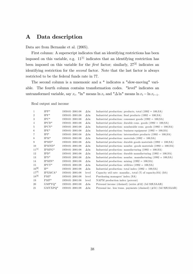
A Data description

Data are from Bernanke et al. (2005).

First column: A superscript indicates that an identifying restrictions has been

imposed on this variable, e.g. 11[1] indicates that an identifying restriction has

been imposed on this variable for the �rst factor; similarly, 27[2] indicates an

identifying restriction for the second factor. Note that the last factor is always

restricted to be the federal funds rate in 77.

The second column is a mnemonic and a * indicates a "slow-moving" vari-

able. The fourth column contains transformation codes. "level" indicates an

untransformed variable, say xt: "ln" means lnxt and "� ln" means lnxt� lnxt�1:

Real output and income

1 IPP* 1959:01�2001:08 � ln Industrial production: products, total (1992 = 100,SA)

2 IPF* 1959:01�2001:08 � ln Industrial production: �nal products (1992 = 100,SA)

3 IPC* 1959:01�2001:08 � ln Industrial production: consumer goods (1992 = 100,SA)

4 IPCD* 1959:01�2001:08 � ln Industrial production: durable cons. goods (1992 = 100,SA)

5 IPCN* 1959:01�2001:08 � ln Industrial production: nondurable cons. goods (1992 = 100,SA)

6 IPE* 1959:01�2001:08 � ln Industrial production: business equipment (1992 = 100,SA)

7 IPI* 1959:01�2001:08 � ln Industrial production: intermediate products (1992 = 100,SA)

8 IPM* 1959:01�2001:08 � ln Industrial production: materials (1992 = 100,SA)

9 IPMD* 1959:01�2001:08 � ln Industrial production: durable goods materials (1992 = 100,SA)

10 IPMND* 1959:01�2001:08 � ln Industrial production: nondur. goods materials (1992 = 100,SA)

11[1] IPMFG* 1959:01�2001:08 � ln Industrial production: manufacturing (1992 = 100,SA)

12 IPD* 1959:01�2001:08 � ln Industrial production: durable manufacturing (1992 = 100,SA)

13 IPN* 1959:01�2001:08 � ln Industrial production: nondur. manufacturing (1992 = 100,SA)

14 IPMIN* 1959:01�2001:08 � ln Industrial production: mining (1992 = 100,SA)

15 IPUT* 1959:01�2001:08 � ln Industrial production: utilities (1992 = 100,SA)

16[9] IP* 1959:01�2001:08 � ln Industrial production: total index (1992 = 100,SA)

17[7] IPXMCA* 1959:01�2001:08 level Capacity util rate: manufac., total (% of capacity,SA) (frb)

18[3] PMI* 1959:01�2001:08 level Purchasing managers�index (SA)

19 PMP* 1959:01�2001:08 level NAPM production index (percent)

20 GMPYQ* 1959:01�2001:08 � ln Personal income (chained) (series #52) (bil 92$,SAAR)

21 GMYXPQ* 1959:01�2001:08 � ln Personal inc. less trans. payments (chained) (#51) (bil 92$,SAAR)

38

(Un)employment and hours

22 LHEL* 1959:01�2001:08 � ln Index of help-wanted advertising in newspapers (1967 = 100;SA)

23[6] LHELX* 1959:01�2001:08 ln Employment: ratio; help-wanted ads: no. unemployed clf

24 LHEM* 1959:01�2001:08 � ln Civilian labor force: employed, total (thous.,SA)

25 LHNAG* 1959:01�2001:08 � ln Civilian labor force: employed, nonag. industries (thous.,SA)

26 LHUR* 1959:01�2001:08 level Unemployment rate: all workers, 16 years and over (%,SA)

27[2] LHU680* 1959:01�2001:08 level Unemploy. by duration: average (mean) duration in weeks (SA)

28 LHU5* 1959:01�2001:08 level Unemploy. by duration: pers unempl. less than 5 wks (thous.,SA)

29 LHU14* 1959:01�2001:08 level Unemploy. by duration: pers unempl. 5 to 14 wks (thous.,SA)

30 LHU15* 1959:01�2001:08 level Unemploy. by duration: pers unempl. 15 wks = (thous.,SA)

31 LHU26* 1959:01�2001:08 level Unemploy. by duration: pers unempl. 15 to 26 wks (thous.,SA)

32 LPNAG* 1959:01�2001:08 � ln Employees on nonag. payrolls: total (thous.,SA)

33 LP* 1959:01�2001:08 � ln Employees on nonag. payrolls: total, private (thous.,SA)

34 LPGD* 1959:01�2001:08 � ln Employees on nonag. payrolls: goods-producing (thous.,SA)

35 LPMI* 1959:01�2001:08 � ln Employees on nonag. payrolls: mining (thous.,SA)

36 LPCC* 1959:01�2001:08 � ln Employees on nonag. payrolls: contract construc. (thous.,SA)

37 LPEM* 1959:01�2001:08 � ln Employees on nonag. payrolls: manufacturing (thous.,SA)

38 LPED* 1959:01�2001:08 � ln Employees on nonag. payrolls: durable goods (thous.,SA)

39 LPEN* 1959:01�2001:08 � ln Employees on nonag. payrolls: nondurable goods (thous.,SA)

40 LPSP* 1959:01�2001:08 � ln Employees on nonag. payrolls: service-producing (thous.,SA)

41 LPTU* 1959:01�2001:08 � ln Employees on nonag. payrolls: trans. and public util. (thous.,SA)

42 LPT* 1959:01�2001:08 � ln Employees on nonag. payrolls: wholesale and retail (thous.,SA)

43 LPFR* 1959:01�2001:08 � ln Employees on nonag. payrolls: �nance, ins. and real est (thous.,SA)

44 LPS* 1959:01�2001:08 � ln Employees on nonag. payrolls: services (thous.,SA)

45 LPGOV* 1959:01�2001:08 � ln Employees on nonag. payrolls: government (thous.,SA)

46 LPHRM* 1959:01�2001:08 level Avg. weekly hrs. of production wkrs.: manufacturing (sa)

47[4] LPMOSA* 1959:01�2001:08 level Avg. weekly hrs. of prod. wkrs.: mfg., overtime hrs. (sa)

48 PMEMP* 1959:01�2001:08 level NAPM employment index (percent)

Consumption

49 GMCQ* 1959:01�2001:08 � ln Pers cons exp (chained)� total (bil 92$,SAAR)

50[8] GMCDQ* 1959:01�2001:08 � ln Pers cons exp (chained)� tot. dur. (bil 96$,SAAR)

51 GMCNQ* 1959:01�2001:08 � ln Pers cons exp (chained)� nondur. (bil 92$,SAAR)

52 GMCSQ* 1959:01�2001:08 � ln Pers cons exp (chained)� services (bil 92$,SAAR)

53 GMCANQ* 1959:01�2001:08 � ln Personal cons expend (chained)� new cars (bil 96$,SAAR)

Housing starts and sales

54 HSFR 1959:01�2001:08 ln Housing starts: nonfarm (1947�1958); tot.

55 HSNE 1959:01�2001:08 ln Housing starts: northeast (thous.u.)s.a.

56 HSMW 1959:01�2001:08 ln Housing starts: midwest (thous.u.)s.a.

57 HSSOU 1959:01�2001:08 ln Housing starts: south (thous.u.)s.a.

58 HSWST 1959:01�2001:08 ln Housing starts: west (thous.u.)s.a.

59 HSBR 1959:01�2001:08 ln Housing authorized: total new priv housing (thous.,SAAR)

60 HMOB 1959:01�2001:08 ln Mobile homes: manufacturers�shipments (thous. of units,SAAR)

39

Real inventories, orders and un�lled orders

61 MNV 1959:01�2001:08 level NAPM inventories index (percent)

62 PMNO 1959:01�2001:08 level NAPM new orders index (percent)

63 PMDEL 1959:01�2001:08 level NAPM vendor deliveries index (percent)

64 MOCMQ 1959:01�2001:08 � ln New orders (net)� consumer goods and materials, 1992 $ (bci)

65 MSONDQ 1959:01�2001:08 � ln New orders, nondefense capital goods, in 1992 $s (bci)

Stock prices

66 FSNCOM 1959:01�2001:08 � ln NYSE composite (12/31/65 = 50)

67 FSPCOM 1959:01�2001:08 � ln S&P�s composite (1941�1943 = 10)

68 FSPIN 1959:01�2001:08 � ln S&P�s industrials (1941�1943 = 10)

69 FSPCAP 1959:01�2001:08 � ln S&P�s capital goods (1941�1943 = 10)

70 FSPUT 1959:01�2001:08 � ln S&P�s utilities (1941�1943 = 10)

71 FSDXP 1959:01�2001:08 level S&P�s composite common stock: dividend yield (% per annum)

72 FSPXE 1959:01�2001:08 level S&P�s composite common stock: price-earnings ratio (%,NSA)

Foreign exchange rates

73 EXRSW 1959:01�2001:08 � ln Foreign exchange rate: Switzerland (Swiss franc per US$)

74 EXRJAN 1959:01�2001:08 � ln Foreign exchange rate: Japan (yen per US$)

75 EXRUK 1959:01�2001:08 � ln Foreign exchange rate: United Kingdom (cents per pound)

76 EXRCAN 1959:01�2001:08 � ln Foreign exchange rate: Canada (Canadian $ per US$)

Interest rates and spreads

77 FYFF 1959:01�2001:08 level Interest rate: federal funds (e¤ective) (% per annum,nsa)

78 FYGM3 1959:01�2001:08 level Interest rate: us tbill,sec mkt,3-mo. (% per ann,nsa)

79 FYGM6 1959:01�2001:08 level Interest rate: us tbill,sec mkt,6-mo. (% per ann,nsa)

80 FYGT1 1959:01�2001:08 level Interest rate: ust const matur., 1-yr. (% per ann,nsa)

81 FYGT5 1959:01�2001:08 level Interest rate: ust const matur., 5-yr. (% per ann,nsa)

82 FYGT10 1959:01�2001:08 level Interest rate: ust const matur., 10-yr. (% per ann,nsa)

83 FYAAAC 1959:01�2001:08 level Bond yield: Moody�s AAA corporate (% per annum)

84 FYBAAC 1959:01�2001:08 level Bond yield: Moody�s BAA corporate (% per annum)

85 SFYGM3 1959:01�2001:08 level Spread fygM3� fy¤

86 SFYGM6 1959:01�2001:08 level Spread fygm6� fy¤

87 SFYGT1 1959:01�2001:08 level Spread fygt1� fy¤

88 SFYGT5 1959:01�2001:08 level Spread fygt5� fy¤

89 SFYGT10 1959:01�2001:08 level Spread fygt10� fy¤

90 SFYAAAC 1959:01�2001:08 level Spread fyaaac� fy¤

91 SFYBAAC 1959:01�2001:08 level Spread fybaac� fy¤

40

Money and credit quantity aggregates

92 FM1 1959:01�2001:08 � ln Money stock: M1 (bil$,SA)

93 FM2 1959:01�2001:08 � ln Money stock: M2 (bil$,SA)

94 FM3 1959:01�2001:08 � ln Money stock: M3 (bil$,SA)

95 FM2DQ 1959:01�2001:08 � ln Money supply� M2 in 1992 $s (bci)

96 FMFBA 1959:01�2001:08 � ln Monetary base, adj for reserve requirement changes (mil$,SA)

97 FMRRA 1959:01�2001:08 � ln Depository inst reserves: total, adj for res. req chgs (mil$,SA)

98 FMRNBA 1959:01�2001:08 � ln Depository inst reserves: nonbor., adj res req chgs (mil$,SA)

99 FCLNQ 1959:01�2001:08 � ln Commercial and indust. loans outstanding in 1992 $s (bci)

100 FCLBMC 1959:01�2001:08 level Wkly rp lg com. banks: net change com and ind. loans (bil$,SAAR)

101 CCINRV 1959:01�2001:08 � ln Consumer credit outstanding nonrevolving g19

Price indexes

102 PMCP 1959:01�2001:08 level NAPM commodity prices index (%)

103 PWFSA* 1959:01�2001:08 � ln PPI: �nished goods (82 = 100,SA)

104 PWFCSA* 1959:01�2001:08 � ln PPI: �nished consumer goods (82 = 100,SA)

105 PWIMSA* 1959:01�2001:08 � ln PPI: intermed mat. sup and components (82 = 100,SA)

106 PWCMSA* 1959:01�2001:08 � ln PPI: crude materials (82 = 100,SA)

107 PSM99Q* 1959:01�2001:08 � ln Index of sensitive materials prices (1990 = 100) (bci-99a)

108 PUNEW* 1959:01�2001:08 � ln CPI-u: all items (82�84 = 100,SA)

109 PU83* 1959:01�2001:08 � ln CPI-u: apparel and upkeep (82�84 = 100,SA)

110 PU84* 1959:01�2001:08 � ln CPI-u: transportation (82�84 = 100,SA)

111 PU85* 1959:01�2001:08 � ln CPI-u: medical care (82�84 = 100,SA)

112[5] PUC* 1959:01�2001:08 � ln CPI-u: commodities (82�84 = 100,SA)

113 PUCD* 1959:01�2001:08 � ln CPI-u: durables (82�84 = 100,SA)

114 PUS* 1959:01�2001:08 � ln CPI-u: services (82�84 = 100,SA)

115 PUXF* 1959:01�2001:08 � ln CPI-u: all items less food (82�84 = 100,SA)

116 PUXHS* 1959:01�2001:08 � ln CPI-u: all items less shelter (82�84 = 100,SA)

117 PUXM* 1959:01�2001:08 � ln CPI-u: all items less medical care (82�84 = 100,SA)

Average hourly earnings

118 LEHCC* 1959:01�2001:08 �ln Avg hr earnings of constr wkrs: construction ($,SA)

119 LEHM* 1959:01�2001:08 �ln Avg hr earnings of prod wkrs: manufacturing ($,SA)

Miscellaneous

120 HHSNTN 1959:01�2001:08 level U. of mich. index of consumer

41

B Appendix: Forecast error variance decompo-

sition

Consider the forecast error of the optimal h�step ahead forecast for the jthobserved variable:

Xj;t+h � Xj;t+hjt =

h�1Xi=1

h�j iW

iet+h�i + �j;t+h

=

h�1Xi=1

iet+h�i + �j;t+h

=KXk=1

(jk;0ek;t+h +jk;1ek;t+h�1 + :::+jk;h�1ek;t+1) + �j;t+h

where et is the orthogonal residual de�ned from the VAR residuals, "t = Pet

where P is the Cholesky factor from the decomposition of the covariance of "tinto Q = PP>: This covariance matrix is further rewritten as explained in section

4.5 as Q = W�eW>; where �e = DD> is diagonal and W = PD�1 has ones

along the diagonal. Moreover, i = �j iW is a N � r matrix and �j;t+h is the

jth idiosyncratic term. The mean square error of�Xj;t+h � Xj;t+hjt

�is denoted

MSE�Xj;t+hjt

�and given by:

MSE�Yj;t+hjt

�=

KXk=1

�2jk;0d

2kk +

2jk;1d

2kk + :::+2jk;h�1d

2kk

�+Rj;j

where d2kk is the (k; k) element of the diagonal matrixDD> andRj;j is the vari-

ance of the jth idiosyncratic term. The proportion of the forecast error variance

at horizon h of variable Xj due to the kth innovation ek;t is given by:

!jk (h) =d2kkPh�1

i=0

�2jk;0 +

2jk;1 + :::+2jk;h�1

�MSE

�Xj;t+hjt

�+Rj;j

42

C Appendix: Kalman �lter, Kalman smoother

and the EM algorithm

C.1 The Kalman �lter

The Kalman �lter is an algorithm for sequentially updating a linear projection

for a dynamic system. Denote the information set X t = fX1; :::; Xtg and byFt+1jt = E [Ft+1j X t] the linear projection of Ft+1 on Xt: The variance is denotedPt+1jt = var (Ft+1j X t) : The Kalman �lter recursions for t = 1; ::; T can then be

written as:

Ft+1jt = �Ftjt�1 +Kt

�Xt � �Ftjt�1

�Pt+1jt = �Ptjt�1L

>t +Q

(11)

where�tn�1

= Xt � �Ftjt�1

P ��tjt�1n�n

= �Ptjt�1�> +R

Ktk�n

= �Ptjt�1�>��Ptjt�1�

> +R��1

Ltk�k

= ��Kt�

C.2 Kalman smoothing

Kalman smoothing reconstructs the full state sequence fF1; ::; FTg given the ob-servations fX1; ::; XTg. Smoothing provides us with more accurate inference onthe state variables since it uses more information than the basic �lter. The

Kalman smoother recursions are based on the e¢ cient smoother by de Jong &

Mackinnon (1988) and de Jong (1989) which is used in Koopman & Shephard

(1992) and given by:

43

FtjT = Ftjt�1 + Ptjt�1�>hP ��tjt�1

i�1�t + Ptjt�1L

>t rt(12)

= Ftjt�1 + Ptjt�1rt�1 (alternatively)

PtjT = Ptjt�1 � Ptjt�1Nt�1Ptjt�1 (13)

Pft;t�1gjT =�I � Ptjt�1Nt�1

�Lt�1Pt�1jt�2, (14)

for t = T � 1; :::; 1 (15)

cov�Ft � FtjT ; Fj � FjjT

�= Ptjt�1L

>t L

>t+1 � � � L>j�1

hI �Nj�1Pjjj�1

i(16)

for j � t

where:

rt�1 = �>hP ��tjt�1

i�1�t + L>t rt; for 1 � t < T and rT = 0

Nt�1 = �>hP ��tjt�1

i�1� + L>t NtL for 1 � t < T and NT = 0

Lt = ��Kt� = �� �Ptjt�1�>hP ��tjt�1

i�1�:

The smoothed residuals given by Koopman (1993) are used in for instance the

Portmanteau test:

"tjT = E ["tj XT ] = FtjT � �Ft�1jT= Q�>rt; t = 1; ::; T (17)

and variance and covariance:

var ("t) = Q�Q�>Nt�Q

cov�"t � "tjT ; "j � "jjT

�= �Q�>L>t+1 � � �L>j�1L>j Nj�Q; j = t+ 1; :::; T

with the convention that L>t � � �L>T�1 = Ir when t = T and L>t � � �L>T�1 = L>T�1when t = T � 1:

44

C.3 The complete data likelihood and the incomplete data

likelihood

Under the Gaussian assumption including F0 � N (�0; P0) and ignoring the con-

stant, the complete data likelihood of equation (4) page 10 assuming a VAR(1)

for simplicity and ignoring � is written as:

�2 lnLF ;X (�) = ln jP0j+ (F0 � �0)> P�10 (F0 � �0)

+T � ln jQj+TXt=1

(Ft � �Ft�1)>Q�1 (Ft � �Ft�1)

+T � ln jRj+TXt=1

(Xt � �Ft)>R�1 (Xt � �Ft)

(18)

given that we can observe the states FT = fF0; ::; FTg as well as the observa-tions XT = fX1; ::; XTg. However, given XT and initial values of the parameterestimates (denoted �(j�1)), the conditional expectation of the complete data like-

lihood can be written as:

Q��j�(j�1)

�= E

��2 lnLF ;X (�)

��XT ;�(j�1) �= ln jP0j+ tr

�P�10

��F0jT � �0

��F0jT � �0

�>+ P0jT

��+T � ln jQj+ tr

�Q�1

�C �B�> � �B> + �A�>

�+T � ln jRj+ tr

"R�1

TXt=1

��Xt � �FtjT

��Xt � �FtjT

�>+ �PtjT�

>�#(19)

where the following moments can be calculated from the Kalman smoother listed

above:

A =PT

t=1

�Ft�1jT F

>t�1jT + Pt�1jT

�B =

PTt=1

�FtjT F

>t�1jT + Pft;t�1gjT

�C =

PTt=1

�FtjT F

>tjT + PtjT

�D =

PTt=1XtF

>tjT E =

PTt=1XtX

>t

A useful trick to arrive at (19) is to consider the decomposition of the true

state variable Ft = FtjT +�Ft � FtjT

�; which explains the terms in for instance

45

C; where:

PtjT = E

��Ft � FtjT

��Ft � FtjT

�>����XT� :The estimator of �� subject to linear restrictions is:

vec (��) = vec�BA�1

�+�A�1 Q

�H>�

�H�

�A�1 Q

�H>�

��1 ��� �H� vec

�BA�1

�(20)

where �� is a %� 1 vector and the restriction matrix H� is of dimension %� r2:

D Appendix: Analytical derivatives of the log

likelihood function

The following is primarily from Jungbacker & Koopman (2008) and Koopman

& Shephard (1992). A key result @ logLY (�)@Q

���Q=Q�

= @Q(�j��)@Q

���Q=Q�

is from Louis

(1982).

Consider the following derivatives of the log likelihood function for the state

space model with incomplete data:

@ logLY (�)

@Q

����Q=Q�

=@Q (�j��)

@Q

����Q=Q�

= Q�1 (S � T �Q)Q�1�12diag

�Q�1 (S � T �Q)Q�1

�where:

S = C �B�> � �B> + �A�>

and where Q is the covariance matrix of the innovation error in the transition

equation:

@ logLY (�)

@�

�����=��

=@Q (�j��)

@�

�����=��

= Q�1 (B � �A)

where � contains the autoregressive parameters in the transition equation. More-

over, the derivative with respect to � is:

46

@ logLY (�)

@�

�����=��

=@Q (�j��)

@�

�����=��

= R�1

TXt=1

ytF>tjT � �C

!

where � is the loading matrix, R is the covariance of the measurement errors,

yt is the data in the panel data set at time t and F>tjT is the smoothed dynamic

factor. Finally, the derivative with respect to the covariance of the measurement

errors is:

@ logLY (�)

@R

����R=R�

=@Q (�j��)

@R

����R=R�

= R�1 (M � T �R)R�1�12diag

�R�1 (M � T �R)R�1

�:

47

Table 1: Akaike information criterion for a given number of factors.number of factors

lags 3 4 5 6 7 8 9 101 - 11.467 - 13.271 - 17.625 - 24.756 - 22.658 - - 30.480 - 43.8012 - 11.634 - 14.151 - 23.221 - 27.482 - 24.302 - 35.706 - 35.812 - 45.5123 - 11.616 - 16.646 - 19.462 - - - 37.692 - 40.605 - 50.2184 - 11.663 - 16.182 - 18.741 - 28.607 - - 36.904 - 38.251 - 48.5535 - 11.562 - - 19.479 - 26.748 - 30.378 - 37.673 - -6 - 11.904 - 15.653 - 20.636 - 26.683 - 24.834 - 38.726 - 37.483 - 48.7337 - 11.784 - 15.918 - 19.039 - - - 37.302 - 37.034 -8 - 10.627 - 14.955 - 18.993 - 28.004 - - 37.888 - -9 - 10.671 - 15.037 - 19.456 - 26.212 - 26.262 - - -10 - 10.670 - 15.257 - 20.138 - 25.987 - 26.582 - - -11 - 10.898 - 15.212 - 19.939 - - - - -12 - 11.459 - 15.112 - - - - - -13 - - 15.045 - 20.121 - - - - -

A bold number represents a minimum.

Table 2: Schwarz information criterion for a given number of factors.number of factors

lags 3 4 5 6 7 8 9 101 - 11.392 - 13.139 - 17.418 - 24.457 - 22.252 - - 29.809 - 42.9722 - 11.485 - 13.886 - 22.806 - 26.885 - 23.490 - 34.645 - 34.469 - 43.8543 - 11.393 - 16.248 - 18.841 - - - 36.100 - 38.590 - 47.7314 - 11.365 - 15.651 - 17.912 - 27.413 - - 34.782 - 35.565 - 45.2375 - 11.189 - - 18.443 - 25.255 - 28.347 - 35.020 - -6 - 11.456 - 14.857 - 19.392 - 24.893 - 22.397 - 35.543 - 33.454 - 43.7597 - 11.262 - 14.990 - 17.588 - - - 33.588 - 32.333 -8 - 10.030 - 13.894 - 17.335 - 25.616 - - 33.643 - -9 - 9.999 - 13.843 - 17.590 - 23.526 - 22.606 - - -10 - 9.924 - 13.930 - 18.066 - 23.002 - 22.520 - - -11 - 10.078 - 13.753 - 17.659 - - - - -12 - 10.563 - 13.520 - - - - - -13 - - 13.320 - 17.426 - - - - -

Table 3: Hannan and Quinn information criterion for a given numberof factors.

number of factorslags 3 4 5 6 7 8 9 101 - 11.438 - 13.219 - 17.544 - 24.639 - 22.499 - - 30.217 - 43.4762 - 11.576 - 14.047 - 23.058 - 27.248 - 23.984 - 35.290 - 35.285 - 44.8623 - 11.529 - 16.490 - 19.219 - - - 37.068 - 39.815 - 49.2434 - 11.546 - 15.974 - 18.416 - 28.139 - - 36.072 - 37.198 - 47.2535 - 11.416 - - 19.073 - 26.163 - 29.582 - 36.633 - -6 - 11.729 - 15.341 - 20.148 - 25.981 - 23.879 - 37.478 - 35.904 - 46.7837 - 11.580 - 15.554 - 18.470 - - - 35.846 - 35.191 -8 - 10.393 - 14.539 - 18.343 - 27.068 - - 36.224 - -9 - 10.408 - 14.569 - 18.724 - 25.159 - 24.829 - - -10 - 10.378 - 14.737 - 19.326 - 24.817 - 24.990 - - -11 - 10.577 - 14.640 - 19.045 - - - - -12 - 11.108 - 14.488 - - - - - -13 - - 14.369 - 19.064 - - - - -

48

Table 4: Multivariate Portmanteau tests.

Test statistics based on smoothed residuals from a VAR(1)h r = 3 r = 4 r = 5 r = 6 r = 7 r = 8 r = 9 r = 101 140:00�

f0:000g218:04�f0:000g

252:36�f0:000g

304:13�f0:000g

312:15�f0:000g

362:92�f0:000g

360:50�f0:000g

384:54�f0:000g

2 161:83�f0:000g

250:56�f0:000g

294:05�f0:000g

363:69�f0:000g

387:10�f0:000g

442:70�f0:000g

450:37�f0:000g

471:28�f0:000g

3 181:62�f0:000g

276:12�f0:000g

329:30�f0:000g

419:71�f0:000g

460:05�f0:000g

505:91�f0:000g

532:32�f0:000g

548:44�f0:000g

4 188:83�f0:000g

296:30�f0:000g

361:72�f0:000g

480:70�f0:000g

531:55�f0:000g

558:04�f0:000g

623:72�f0:000g

630:75�f0:000g

5 210:70�f0:000g

324:65�f0:000g

401:96�f0:000g

535:43�f0:000g

607:16�f0:000g

613:96�f0:000g

731:48�f0:000g

742:25�f0:000g

6 230:42�f0:000g

347:53�f0:000g

444:24�f0:000g

593:32�f0:000g

685:95�f0:000g

675:11�f0:000g

825:78�f0:000g

837:65�f0:000g

7 243:14�f0:000g

368:32�f0:000g

482:16�f0:000g

650:24�f0:000g

755:09�f0:000g

734:22�f0:000g

906:11�f0:000g

922:48�f0:000g

8 288:93�f0:000g

418:07�f0:000g

540:25�f0:000g

732:82�f0:000g

866:36�f0:000g

799:02�f0:000g

1; 024:43�f0:000g

1; 045:57�f0:000g

9 308:38�f0:000g

440:20�f0:000g

573:01�f0:000g

782:47�f0:000g

927:33�f0:000g

849:77�f0:000g

1; 094:50�f0:000g

1; 123:82�f0:000g

10 320:56�f0:000g

459:57�f0:000g

598:82�f0:000g

819:95�f0:000g

991:55�f0:000g

884:62�f0:000g

1; 182:08�f0:000g

1; 210:20�f0:000g

12 344:19�f0:000g

497:36�f0:000g

643:14�f0:000g

869:03�f0:000g

1; 043:41�f0:000g

942:27�f0:000g

1; 272:57�f0:000g

1; 302:48�f0:000g

13 377:01�f0:000g

539:93�f0:000g

702:67�f0:000g

935:97�f0:000g

1; 108:93�f0:000g

1; 011:22�f0:000g

1; 359:05�f0:000g

1; 386:90�f0:000g

14 404:69�f0:000g

576:69�f0:000g

738:00�f0:000g

990:09�f0:000g

1; 174:94�f0:000g

1; 064:53�f0:000g

1; 442:79�f0:000g

1; 470:31�f0:001g

15 425:71�f0:000g

617:82�f0:000g

788:63�f0:000g

1; 040:62�f0:000g

1; 240:25�f0:000g

1; 122:43�f0:000g

1; 515:66�f0:000g

1; 549:43�f0:003g

Test statistics based on smoothed residuals from a VAR(2)h r = 3 r = 4 r = 5 r = 6 r = 7 r = 8 r = 9 r = 101 58:66�

f0:000g59:48�f0:000g

88:26�f0:000g

88:05�f0:000g

120:09�f0:000g

127:29�f0:000g

150:73�f0:000g

158:01�f0:000g

2 69:11�f0:000g

72:03�f0:000g

105:40�f0:000g

110:30�f0:003g

162:96�f0:000g

178:34�f0:002g

227:23�f0:001g

220:72f0:150g

3 73:66�f0:000g

90:34�f0:000g

138:02�f0:000g

161:16�f0:001g

222:99�f0:000g

240:76�f0:010g

313:06�f0:002g

297:66f0:527g

4 93:25�f0:000g

113:36�f0:000g

180:74�f0:000g

209:08�f0:000g

287:91�f0:000g

303:90�f0:021g

397:97�f0:003g

393:07f0:588g

5 118:35�f0:000g

139:77�f0:000g

218:54�f0:000g

250:64�f0:000g

342:75�f0:000g

360:20f0:060g

466:35�f0:019g

457:32f0:915g

6 128:73�f0:000g

154:08�f0:000g

244:03�f0:000g

284:04�f0:001g

391:37�f0:000g

402:32f0:250g

519:99f0:139g

526:91f0:986g

7 166:25�f0:000g

185:86�f0:000g

277:94�f0:000g

333:40�f0:000g

475:13�f0:000g

477:40f0:163g

609:53f0:105g

633:67f0:965g

8 185:63�f0:000g

204:51�f0:000g

299:97�f0:000g

366:12�f0:001g

521:55�f0:000g

528:66f0:296g

663:27f0:330g

688:64f0:998g

9 193:90�f0:000g

221:42�f0:000g

322:41�f0:000g

393:23�f0:005g

570:79�f0:000g

579:33f0:453g

731:97f0:462g

782:77f0:998g

10 216:72�f0:000g

246:77�f0:000g

352:08�f0:000g

439:60�f0:003g

624:22�f0:000g

612:92f0:773g

810:22f0:491g

858:89f1:000g

12 242:06�f0:000g

279:14�f0:000g

402:61�f0:000g

492:10�f0:001g

679:98�f0:000g

658:83f0:887g

872:45f0:665g

943:96f1:000g

13 257:49�f0:000g

294:25�f0:000g

421:62�f0:000g

532:21�f0:001g

730:13�f0:000g

711:68f0:927g

935:29f0:796g

1; 020:73f1:000g

14 270:65�f0:000g

319:49�f0:000g

460:12�f0:000g

567:78�f0:001g

782:21�f0:000g

757:77f0:969g

995:82f0:895g

1; 084:72f1:000g

The rows represent test statistics of residual autocorrelation up to order h. H0: Residualautocorrelation up to lag h is zero. p-values in fg: � indicates rejection on 5 pct. level.

49

Table 5: Multivariate Portmanteau tests.

Test statistics based on smoothed residuals from a VAR(3)h r = 3 r = 4 r = 5 r = 6 r = 7 r = 8 r = 9 r = 101 26:30�

f0:002g52:15�f0:000g

49:16�f0:003g

fa iled max. iterations 64:70f0:452g

100:79f0:068g

97:81f0:543g

2 31:19�f0:027g

71:02�f0:000g

87:50�f0:001g

- - 102:85f0:950g

178:52f0:178g

160:17f0:983g

3 46:73�f0:011g

92:27�f0:000g

118:99�f0:001g

- - 156:50f0:972g

247:82f0:402g

239:47f0:996g

4 64:98�f0:002g

106:51�f0:001g

147:55�f0:001g

- - 194:08f0:999g

306:45f0:751g

299:03f1:000g

5 74:80�f0:004g

123:08�f0:001g

174:07�f0:003g

- - 224:64f1:000g

344:81f0:986g

367:33f1:000g

6 99:72�f0:000g

155:54�f0:000g

212:95�f0:001g

- - 284:73f1:000g

419:23f0:987g

446:80f1:000g

7 114:30�f0:000g

166:46�f0:001g

231:74�f0:003g

- - 328:48f1:000g

468:23f0:999g

496:79f1:000g

8 120:55�f0:000g

185:85�f0:001g

260:84�f0:003g

- - 370:56f1:000g

527:45f1:000g

574:34f1:000g

9 134:73�f0:000g

199:94�f0:001g

279:82�f0:008g

- - 404:49f1:000g

593:54f1:000g

636:62f1:000g

10 157:52�f0:000g

212:42�f0:004g

301:64�f0:014g

- - 446:82f1:000g

653:77f1:000g

709:65f1:000g

11 170:53�f0:000g

239:61�f0:001g

345:27�f0:003g

- - 490:68f1:000g

708:49f1:000g

783:20f1:000g

12 183:29�f0:000g

253:33�f0:002g

377:71�f0:002g

- - 527:04f1:000g

763:42f1:000g

841:09f1:000g

Test statistics based on smoothed residuals from a VAR(4)h r = 3 r = 4 r = 5 r = 6 r = 7 r = 8 r = 9 r = 101 21:00�

f0:013g28:82�f0:025g

60:72�f0:000g

24:66f0:924g

- 64:46f0:460g

125:89�f0:001g

105:20f0:341g

2 37:59�f0:004g

43:90f0:078g

92:43�f0:000g

52:71f0:957g

- 94:92f0:987g

171:86f0:283g

176:64f0:882g

3 60:32�f0:000g

63:89f0:062g

121:33�f0:001g

75:17f0:993g

- 141:01f0:998g

216:79f0:886g

230:63f0:999g

4 67:40�f0:001g

75:83f0:148g

139:58�f0:006g

89:52f1:000g

- 166:00f1:000g

256:54f0:998g

288:91f1:000g

5 90:86�f0:000g

104:85�f0:033g

175:20�f0:002g

126:35f0:999g

- 219:22f1:000g

314:99f1:000g

351:50f1:000g

6 103:86�f0:000g

110:88f0:142g

191:64�f0:012g

140:07f1:000g

- 257:89f1:000g

372:87f1:000g

404:90f1:000g

7 109:69�f0:000g

126:97f0:158g

218:54�f0:014g

162:72f1:000g

- 292:05f1:000g

447:16f1:000g

478:20f1:000g

8 121:38�f0:000g

145:09f0:143g

239:23�f0:030g

185:96f1:000g

- 323:48f1:000g

512:27f1:000g

535:13f1:000g

9 143:21�f0:000g

165:07f0:110g

265:68�f0:033g

217:70f1:000g

- 363:93f1:000g

570:38f1:000g

599:09f1:000g

10 155:96�f0:000g

196:74�f0:026g

314:68�f0:003g

267:49f1:000g

- 412:06f1:000g

635:52f1:000g

677:01f1:000g

11 167:10�f0:000g

212:70�f0:031g

332:92�f0:010g

284:29f1:000g

- 447:43f1:000g

685:14f1:000g

728:51f1:000g

The rows represent test statistics of residual autocorrelation up to order h. H0: Residualautocorrelation up to lag h is zero. p-values in fg: � indicates rejection on 5 pct. level.Unreported numbers show that a VAR(5) �xes the residual autocorrelation for r = 5,whereas for r = 3, the problem remains.

50

Table 6: Forecast error variance decompositions for key macroeco-nomic variables.

F (8; 1) F (8; 2) F (8; 3) F (8; 4) F (8; 5) F (8; 6) F (8; 7) FFR) F� total Idio:6m 0:06 0:03 0:02 0:06 0:07 0:07 0:04 0:04 0:39 0:6112m 0:06 0:03 0:04 0:07 0:07 0:06 0:06 0:05 0:43 0:5724m 0:06 0:03 0:06 0:07 0:07 0:06 0:08 0:05 0:47 0:5360m 0:06 0:03 0:10 0:07 0:07 0:05 0:09 0:04 0:51 0:49

60-month horizon F (8; 1) F (8; 2) F (8; 3) F (8; 4) F (8; 5) F (8; 6) F (8; 7) FFR77) Federal funds rate 0:03 0:06 0:35 0:23 0:03 0:08 0:19 0:0316) IP: total index 0:50 0:03 0:05 0:11 0:03 0:10 0:09 0:07108) CPI-U: all items 0:02 0:07 0:20 0:09 0:42 0:02 0:09 0:0278) US Tbill, 3m. 0:03 0:06 0:35 0:20 0:03 0:10 0:18 0:0281) Tbond const 5yr. 0:04 0:07 0:38 0:17 0:05 0:18 0:09 0:0196) Monetary base 0:00 0:02 0:02 0:02 0:01 0:01 0:03 0:0093) Money stock: M2 0:01 0:06 0:03 0:01 0:03 0:03 0:06 0:0174) FX: Japan 0:01 0:01 0:01 0:00 0:00 0:01 0:03 0:00102) NAPM commodity prices 0:02 0:06 0:17 0:05 0:10 0:07 0:11 0:0617) Capacity util rate 0:03 0:01 0:17 0:12 0:09 0:04 0:21 0:1249) Pers cons exp: total 0:01 0:00 0:01 0:01 0:04 0:00 0:01 0:0050) Pers cons exp: tot. dur 0:01 0:00 0:01 0:00 0:01 0:00 0:01 0:0051) Pers cons exp: nondur. 0:01 0:00 0:01 0:00 0:03 0:00 0:01 0:0026) Unempl. rate: all wrks 0:05 0:02 0:21 0:10 0:19 0:05 0:21 0:1548) NAPM Empl. Index 0:02 0:01 0:20 0:12 0:07 0:10 0:22 0:15118) Avg hr earnings constr. 0:01 0:01 0:01 0:00 0:01 0:00 0:01 0:0054) Housing starts: nonfarm 0:02 0:07 0:14 0:04 0:07 0:04 0:20 0:0662) NAPM new orders 0:03 0:02 0:18 0:10 0:04 0:11 0:23 0:1471) SP500: dividend 0:05 0:08 0:30 0:03 0:08 0:03 0:14 0:02120) Consumer expec. (Mich.) 0:02 0:05 0:15 0:09 0:21 0:03 0:04 0:05

The upper panel illustrates the total fraction that the eight factors can explain of theforecast error variance at varying horizons. "Idio." means idiosyncratic variance. FFRmeans federal funds rate, which is the shock in focus. The lower table shows the 60-month ahead forecast error variance decomposition for key macroeconomic variables.

51

Figure 1: The panel information criterion ICp3 of Bai & Ng (2002).The criterion does not provide information about the number of lags in the VAR sothe criterion as a function of the number of static factors, r; is calculated for a givennumber of lags. On top of each bar the number of factors is plotted. Eight factorsseem to be a good choice when model parsimony is taken into account.

33

33

33

3

33

33

3

44

44

44

44

44

44

55

55

55

55

55

55

6

66

6

66

6

66

77

7

7

77

8

88

88

88

8

99

99

99

10

1010

1010

- 0.500 - 0.450 - 0.400 - 0.350 - 0.300 - 0.250 - 0.200 - 0.150 - 0.100 - 0.050 -

12

34

56

78

910

1112

13

Num

ber

of la

gs

criterion value IC[p3]

52

Figure 2: Adjusted average R2 of all variables in the panel for allmodels.For each FAVAR model with r factors and p lags in the VAR, the �R2 is calculated.The number on top of each bar represents the number of lags in the VAR with rfactors. Note how the incremental value of �R2 diminishes as more factors are added.

Adjusted R-square in %

1

2

3

4

5

6

7

8

9

10

11

12

1

2

3

4

6

7

8

9

10

11

12

13

1

2

3

4

5

6

7

8

9

10

11

13

1

2

4

5

6

8

9

10

12

1

2

5

6

9

10

1

2

3

4

5

6

7

8

1

2

3

4

6

7

1

2

3

4

6

0 10 20 30 40 50 60

num

ber

of st

atic

fact

ors (

r)(s

mal

l num

bers

on

top

of e

ach

bar r

epre

sent

s the

num

ber o

f lag

s)

10

9

8

7

6

5

4

3

53

Figure3:

R2foreachvariable:Meanofthe"15best","15medium"and"15worst"performingmodels.

0102030405060708090100

R−square in percent

1) IP: products, total2) IP: final products3) IP: consumer 4) IP: durable cons.5) IP: nondur. cons.6) IP: bus. Equip 7) IP: intermediate 8) IP: materials 9) IP: durable goods10) IP: nondur. goods11) IP: manufacturing12) IP: dur. manuf13) IP: nondur. manuf.14) IP: mining 15) IP: utilities16) IP: total index17) Capacity util rate18) Pmi19) NAPM prod.20) Pers. Income 21) Pers. Inc. − trans.22) Help−wated 23) Empl. Help−wanted24) Civ. Labor: empl.,25) Civilian labor: empl.,26) Unempl. Rate: all wrks27) Unemp dur: mean28) Unemp dur. < 5 w.29) Unemp dur. 5−14 w30) Unemp dur. 15+ w31) Unemp dur. 15−26 w32) Nonag payrl.: total33) Nonag payrl.: total,34) Nonag payrl.: goods35) Nonag payrl.: mining36) Nonag payrl.: contract37) Nonag payrl.: manuf38) Nonag payrl.: durable39) Nonag payrl.: nondur40) Nonag payrl.: service41) Nonag payrl.: trans.42) Nonag payrl.: sale43) Nonag payrl.: finance44) Nonag payrl.: services45) Nonag payrl.: gov.46) Avg. Wkly hrs. prod47) Avg. Wkly overtime prod48) NAPM Empl. Index49) Pers cons exp: total50) Pers cons exp: tot.51) Pers cons exp: nondur.52) Pers cons exp: services53) Pers cons exp: new cars54) Housing starts: nonfarm 55) Housing starts: N.E56) Housing starts: M.W 57) Housing starts: S58) Housing starts: S 59) Housing auth. Tot new60) Mobile homes61) NAPM inventories62) NAPM new orders 63) NAPM vendor deliv. 64) New orders: cons goods65) New orders: nondefense 66) NYSE: composite67) SP500 composite68) SP500 industrials69) SP500 capital70) SP500 utilities71) SP500: dividend 72) SP500: price earnings 73) FX : Switzerland74) FX : Japan75) FX : U.K76) FX : Canada77) Federal funds78) US Tbill, 3m.79) US Tbill, 6m.80) Tbond const 1yr.81) Tbond const 5yr.82) Tbond const 10yr.83) Bond yield: Moody AAA84) Bond yield: Moody BAA85) Spread 3m – fed funds 86) Spread 6m – fed funds 87) Spread 1y – fed funds88) Spread 5y – fed funds89) Spread 10y – fed funds90) Spread AAA – fed funds91) Spread BAA – fed funds92) Money stock: M1 93) Money stock: M2 94) Money stock: M3 95) Money supply−−−M2 199296) Monetary base97) Depository inst reserves98) Dep. Inst. Res. Nonbor.99) Comm. and indust. Loans100) Wkly rp lg com.101) Cons credit outst.102) NAPM commodity prices 103) PPI: finished104) PPI: finished105) PPI: intermed106) PPI: crude107) Index of sensitive mat.108) CPI−U: all items109) CPI−U: apparel, upkeep110) CPI−U: transportation111) CPI−U: medical care112) CPI−U: commodities113) CPI−U: durables114) CPI−U: services115) CPI−U: less food116) CPI−U: less shelter117) CPI−U: less medical118) Avg hr earnings constr.119) Avg hr earnings manuf.120) Consumer expec. (Mich.)

R−

squa

re fo

r bo

ttom

−15

of a

ll m

odel

s (m

ean)

R−

squa

re fo

r m

id−

15 o

f all

mod

els

(mea

n)R

−sq

uare

for

top−

15 o

f all

mod

els

(mea

n)

54

Figure 4: Autocorrelation functions for the preferred speci�cation ver-sus a VAR(1).

E:\phd\paper1\graphs\givewin\Newlag1vsLagBestACFwithr4p7.eps 09/04/08 08:13:41

Page: 1 of 1

0 5 10

0

1ACF-r3p1(3) ACF-r3p7(3)

0 5 10

0

1ACF-r4p1(4) ACF-r4p7(4)

0 5 10

0

1ACF-r5p1(5) ACF-r5p6(5)

0 5 10

0

1ACF-r6p1(6) ACF-r6p4(6)

0 5 10

0

1ACF-r7p1(7) ACF-r7p5(7)

0 5 10

0

1ACF-r8p1(8) ACF-r8p3(8)

0 5 10

0

1ACF-r9p1(9) ACF-r9p3(9)

0 5 10

0

1ACF-r10p1(10) ACF-r10p2(10)

The smoothed residual autocorrelation functions for the preferred speci�cations forFAVARs with 3,4,...,10 factors versus their VAR(1) counterpart are plotted to em-phasize that VAR(1) dynamics are not su¢ cient for whiteness in the monetary policyfactor residuals. Unreported results show that there is virtually no di¤erence in theautocorrelation function for r4p7(4) versus BBE-EM version r4p13(4).

55

Figure 5: R2 for the preferred model versus the BBE-EM andBernanke, Boivin and Eliaz.

0102030405060708090100

R−square in percent

1) IP: products, total2) IP: final products3) IP: consumer 4) IP: durable cons.5) IP: nondur. cons.6) IP: bus. Equip 7) IP: intermediate 8) IP: materials 9) IP: durable goods10) IP: nondur. goods11) IP: manufacturing12) IP: dur. manuf13) IP: nondur. manuf.14) IP: mining 15) IP: utilities16) IP: total index17) Capacity util rate18) Pmi19) NAPM prod.20) Pers. Income 21) Pers. Inc. − trans.22) Help−wated 23) Empl. Help−wanted24) Civ. Labor: empl.,25) Civilian labor: empl.,26) Unempl. Rate: all wrks27) Unemp dur: mean28) Unemp dur. < 5 w.29) Unemp dur. 5−14 w30) Unemp dur. 15+ w31) Unemp dur. 15−26 w32) Nonag payrl.: total33) Nonag payrl.: total,34) Nonag payrl.: goods35) Nonag payrl.: mining36) Nonag payrl.: contract37) Nonag payrl.: manuf38) Nonag payrl.: durable39) Nonag payrl.: nondur40) Nonag payrl.: service41) Nonag payrl.: trans.42) Nonag payrl.: sale43) Nonag payrl.: finance44) Nonag payrl.: services45) Nonag payrl.: gov.46) Avg. Wkly hrs. prod47) Avg. Wkly overtime prod48) NAPM Empl. Index49) Pers cons exp: total50) Pers cons exp: tot.51) Pers cons exp: nondur.52) Pers cons exp: services53) Pers cons exp: new cars54) Housing starts: nonfarm 55) Housing starts: N.E56) Housing starts: M.W 57) Housing starts: S58) Housing starts: S 59) Housing auth. Tot new60) Mobile homes61) NAPM inventories62) NAPM new orders 63) NAPM vendor deliv. 64) New orders: cons goods65) New orders: nondefense 66) NYSE: composite67) SP500 composite68) SP500 industrials69) SP500 capital70) SP500 utilities71) SP500: dividend 72) SP500: price earnings 73) FX : Switzerland74) FX : Japan75) FX : U.K76) FX : Canada77) Federal funds78) US Tbill, 3m.79) US Tbill, 6m.80) Tbond const 1yr.81) Tbond const 5yr.82) Tbond const 10yr.83) Bond yield: Moody AAA84) Bond yield: Moody BAA85) Spread 3m – fed funds 86) Spread 6m – fed funds 87) Spread 1y – fed funds88) Spread 5y – fed funds89) Spread 10y – fed funds90) Spread AAA – fed funds91) Spread BAA – fed funds92) Money stock: M1 93) Money stock: M2 94) Money stock: M3 95) Money supply−−−M2 199296) Monetary base97) Depository inst reserves98) Dep. Inst. Res. Nonbor.99) Comm. and indust. Loans100) Wkly rp lg com.101) Cons credit outst.102) NAPM commodity prices 103) PPI: finished104) PPI: finished105) PPI: intermed106) PPI: crude107) Index of sensitive mat.108) CPI−U: all items109) CPI−U: apparel, upkeep110) CPI−U: transportation111) CPI−U: medical care112) CPI−U: commodities113) CPI−U: durables114) CPI−U: services115) CPI−U: less food116) CPI−U: less shelter117) CPI−U: less medical118) Avg hr earnings constr.119) Avg hr earnings manuf.120) Consumer expec. (Mich.)

BB

E−

EM

mod

el (

r4p1

3): 4

fact

ors,

13

lags

Pre

ferr

ed F

AV

AR

(r8

p3):

8 fa

ctor

s, 3

lags

star

s: B

erna

nke,

Boi

vin

& E

liasz

(20

05)

56

Figure6:Thetimeseriesoffactors1-4from

thepreferred

modelversusrelatedobserved

variables.

−6

−4

−20246

r8p3(1)F

acto

r: r

8p3(

1) v

ersu

s IP

: man

ufac

turin

g (

11)

and

IP: t

otal

inde

x (

16)

Jan58

Sep59

May61

Feb63

Oct64

Jun66

Mar68

Nov69

Aug71

Apr73

Dec74

Sep76

May78

Jan80

Oct81

Jun83

Feb85

Nov86

Jul88

Apr90

Dec91

Aug93

May95

Jan97

Sep98

Jun00

−6

−4

−2

0246

IP: manufacturing (11) and IP: total index (16)

F

acto

r: r

8p3(

1)IP

: man

ufac

turin

g (

11)

IP: t

otal

inde

x (

16)

−4

−3

−2

−10123

r8p3(2)Fac

tor:

r8p

3(2)

ver

sus

Une

mp

dur:

mea

n (

27)

and

Spr

ead

BA

A –

fed

fund

s (

91)

Jan58

Sep59

May61

Feb63

Oct64

Jun66

Mar68

Nov69

Aug71

Apr73

Dec74

Sep76

May78

Jan80

Oct81

Jun83

Feb85

Nov86

Jul88

Apr90

Dec91

Aug93

May95

Jan97

Sep98

Jun00

−4

−3

−2

−1

0123

Unemp dur: mean (27) and Spread BAA – fed funds (91)

F

acto

r: r

8p3(

2)

Une

mp

dur:

mea

n (

27)

Spr

ead

BA

A –

fed

fund

s (

91)

−4

−3

−2

−10123

r8p3(3)

Fac

tor:

r8p

3(3)

ver

sus

Pm

i (1

8) a

nd N

AP

M n

ew o

rder

s (

62)

Jan58

Sep59

May61

Feb63

Oct64

Jun66

Mar68

Nov69

Aug71

Apr73

Dec74

Sep76

May78

Jan80

Oct81

Jun83

Feb85

Nov86

Jul88

Apr90

Dec91

Aug93

May95

Jan97

Sep98

Jun00

−4

−3

−2

−1

0123

Pmi (18) and NAPM new orders (62)

F

acto

r: r

8p3(

3)P

mi

(18)

NA

PM

new

ord

ers

(62

)

−3

−2

−10123

r8p3(4)

Fac

tor:

r8p

3(4)

ver

sus

Avg

. Wkl

y ov

ertim

e pr

od (

47)

and

(min

us)

SP

500:

div

iden

d (

71)

Jan58

Sep59

May61

Feb63

Oct64

Jun66

Mar68

Nov69

Aug71

Apr73

Dec74

Sep76

May78

Jan80

Oct81

Jun83

Feb85

Nov86

Jul88

Apr90

Dec91

Aug93

May95

Jan97

Sep98

Jun00

−3

−2

−1

0123

Avg. Wkly overtime prod (47) and (minus) SP500: dividend (71)

F

acto

r: r

8p3(

4)A

vg. W

kly

over

time

prod

(47

)(m

inus

) S

P50

0: d

ivid

end

(71

)

Sha

ded

bars

rep

rese

nt N

BE

R−

date

d re

cess

ions

57

Figure7:Thetimeseriesoffactors5-8from

thepreferred

modelversusrelatedobserved

variables.

−2

−101234

r8p3(8)

Fac

tor:

r8p

3(8)

ver

sus

Fed

eral

fund

s (

77)

and

Tbo

nd c

onst

10y

r. (

82)

Jan58

Sep59

May61

Feb63

Oct64

Jun66

Mar68

Nov69

Aug71

Apr73

Dec74

Sep76

May78

Jan80

Oct81

Jun83

Feb85

Nov86

Jul88

Apr90

Dec91

Aug93

May95

Jan97

Sep98

Jun00

−2

−1

01234

Federal funds (77) and Tbond const 10yr. (82)

F

acto

r: r

8p3(

8)F

eder

al fu

nds

(77

)T

bond

con

st 1

0yr.

(82

)

−4

−3

−2

−1012

r8p3(7)

Fac

tor:

r8p

3(7)

ver

sus

Cap

acity

util

rat

e (

17)

and

Spr

ead

BA

A –

fed

fund

s (

91)

Jan58

Sep59

May61

Feb63

Oct64

Jun66

Mar68

Nov69

Aug71

Apr73

Dec74

Sep76

May78

Jan80

Oct81

Jun83

Feb85

Nov86

Jul88

Apr90

Dec91

Aug93

May95

Jan97

Sep98

Jun00

−4

−3

−2

−1

012

Capacity util rate (17) and Spread BAA – fed funds (91)

Fac

tor:

r8p

3(7)

Cap

acity

util

rat

e (

17)

Spr

ead

BA

A –

fed

fund

s (

91)

−4

−3

−2

−1012

r8p3(6)

Fac

tor:

r8p

3(6)

ver

sus

Em

pl. H

elp−

wan

ted

(23

) an

d (m

inus

) U

nem

pl. R

ate:

all

wrk

s (

26)

Jan58

Sep59

May61

Feb63

Oct64

Jun66

Mar68

Nov69

Aug71

Apr73

Dec74

Sep76

May78

Jan80

Oct81

Jun83

Feb85

Nov86

Jul88

Apr90

Dec91

Aug93

May95

Jan97

Sep98

Jun00

−4

−3

−2

−1

012

Empl. Help−wanted (23) and (minus) Unempl. Rate: all wrks (26)

F

acto

r: r

8p3(

6)

Em

pl. H

elp−

wan

ted

(23

)(m

inus

) U

nem

pl. R

ate:

all

wrk

s (

26)

−5

−4

−3

−2

−10123456

r8p3(5)

Fac

tor:

r8p

3(5)

ver

sus

CP

I−U

: all

item

s (

108)

and

CP

I−U

: com

mod

ities

(11

2)

Jan58

Sep59

May61

Feb63

Oct64

Jun66

Mar68

Nov69

Aug71

Apr73

Dec74

Sep76

May78

Jan80

Oct81

Jun83

Feb85

Nov86

Jul88

Apr90

Dec91

Aug93

May95

Jan97

Sep98

Jun00

−5

−4

−3

−2

−1

0123456

CPI−U: all items (108) and CPI−U: commodities (112)

F

acto

r: r

8p3(

5)C

PI−

U: a

ll ite

ms

(10

8)C

PI−

U: c

omm

oditi

es (

112)

Sha

ded

bars

rep

rese

nt N

BE

R−

date

d re

cess

ions

58

Figure 8: "Industrial production factor" and "unemployment factor".

0 5 10 15 20 25 30 35 40 45 50 55 60 65 70 75 80 85 90 95 100 105 110 115 120−1

−0.8

−0.6

−0.4

−0.2

0

0.2

0.4

0.6

0.8

1

Cor

rela

tion.

real output and income (Un)employment/hours Cons Hous. Inv/orders Stocks FX Interest rates Money agg. Price indices Earn. Misc.

Major categories of the 120 variables in the panel. See appendix.1

Correlation between factor 1 and each of the variables as a function of (�,Q,�).

0 5 10 15 20 25 30 35 40 45 50 55 60 65 70 75 80 85 90 95 100 105 110 115 120−1

−0.8

−0.6

−0.4

−0.2

0

0.2

0.4

0.6

0.8

1

Cor

rela

tion.

real output and income (Un)employment/hours Cons Hous. Inv/orders Stocks FX Interest rates Money agg. Price indices Earn. Misc.

Major categories of the 120 variables in the panel. See appendix.2

Correlation between factor 2 and each of the variables as a function of (�,Q,�).

59

Figure 9: "NAPM factor" and "(overtime)hours factor".

0 5 10 15 20 25 30 35 40 45 50 55 60 65 70 75 80 85 90 95 100 105 110 115 120−1

−0.8

−0.6

−0.4

−0.2

0

0.2

0.4

0.6

0.8

1

Cor

rela

tion.

real output and income (Un)employment/hours Cons Hous. Inv/orders Stocks FX Interest rates Money agg. Price indices Earn. Misc.

Major categories of the 120 variables in the panel. See appendix.3

Correlation between factor 3 and each of the variables as a function of (�,Q,�).

0 5 10 15 20 25 30 35 40 45 50 55 60 65 70 75 80 85 90 95 100 105 110 115 120−1

−0.8

−0.6

−0.4

−0.2

0

0.2

0.4

0.6

0.8

1

Cor

rela

tion.

real output and income (Un)employment/hours Cons Hous. Inv/orders Stocks FX Interest rates Money agg. Price indices Earn. Misc.

Major categories of the 120 variables in the panel. See appendix.4

Correlation between factor 4 and each of the variables as a function of (�,Q,�).

60

Figure 10: "In�ation factor" and "employment factor".

0 5 10 15 20 25 30 35 40 45 50 55 60 65 70 75 80 85 90 95 100 105 110 115 120−1

−0.8

−0.6

−0.4

−0.2

0

0.2

0.4

0.6

0.8

1

Cor

rela

tion.

real output and income (Un)employment/hours Cons Hous. Inv/orders Stocks FX Interest rates Money agg. Price indices Earn. Misc.

Major categories of the 120 variables in the panel. See appendix.5

Correlation between factor 5 and each of the variables as a function of (�,Q,�).

0 5 10 15 20 25 30 35 40 45 50 55 60 65 70 75 80 85 90 95 100 105 110 115 120−1

−0.8

−0.6

−0.4

−0.2

0

0.2

0.4

0.6

0.8

1

Cor

rela

tion.

real output and income (Un)employment/hours Cons Hous. Inv/orders Stocks FX Interest rates Money agg. Price indices Earn. Misc.

Major categories of the 120 variables in the panel. See appendix.6

Correlation between factor 6 and each of the variables as a function of (�,Q,�).

61

Figure 11: "Capacity utilization factor" and "Monetary policy factor".

0 5 10 15 20 25 30 35 40 45 50 55 60 65 70 75 80 85 90 95 100 105 110 115 120−1

−0.8

−0.6

−0.4

−0.2

0

0.2

0.4

0.6

0.8

1

Cor

rela

tion.

real output and income (Un)employment/hours Cons Hous. Inv/orders Stocks FX Interest rates Money agg. Price indices Earn. Misc.

Major categories of the 120 variables in the panel. See appendix.7

Correlation between factor 7 and each of the variables as a function of (�,Q,�).

0 5 10 15 20 25 30 35 40 45 50 55 60 65 70 75 80 85 90 95 100 105 110 115 120−1

−0.8

−0.6

−0.4

−0.2

0

0.2

0.4

0.6

0.8

1

Cor

rela

tion.

real output and income (Un)employment/hours Cons Hous. Inv/orders Stocks FX Interest rates Money agg. Price indices Earn. Misc.

Major categories of the 120 variables in the panel. See appendix.8

Correlation between factor 8 and each of the variables as a function of (�,Q,�).

62

Figure12:Impulseresponsesinstandarddeviationstoa25basispointmonetarypolicyshock.

012

2436

48−

0.1

−0.

050

0.050.1

0.150.2

0.25

77)

Fed

eral

fund

s

mon

ths

012

2436

48−

0.8

−0.

7

−0.

6

−0.

5

−0.

4

−0.

3

−0.

2

−0.

10

0.1

16)

IP: t

otal

inde

x

mon

ths

012

2436

48−

0.8

−0.

6

−0.

4

−0.

20

0.2

0.4

0.6

0.8

108)

CP

I−U

: all

item

s

mon

ths

012

2436

48−

0.06

−0.

04

−0.

020

0.02

0.04

0.06

0.080.1

0.12

0.14

26)

Une

mpl

. Rat

e: a

ll w

rks

mon

ths

Fac

tor

mod

el: r

4p13

Fac

tor

mod

el: r

4p7

Fac

tor

mod

el: r

5p6

Fac

tor

mod

el: r

6p4

Fac

tor

mod

el: r

7p5

Fac

tor

mod

el: r

8p3

Fac

tor

mod

el: r

9p3

012

2436

48−

0.4

−0.

20

0.2

0.4

0.6

0.81

1.2

96)

Mon

etar

y ba

se

mon

ths

012

2436

48−

0.2

−0.

15

−0.

1

−0.

050

0.050.1

0.15

102)

NA

PM

com

mod

ity p

rices

mon

ths

012

2436

48−

0.2

−0.

15

−0.

1

−0.

050

0.050.1

0.15

17)

Cap

acity

util

rat

e

mon

ths

012

2436

48−

0.5

−0.

4

−0.

3

−0.

2

−0.

10

0.1

0.2

118)

Avg

hr

earn

ings

con

str.

mon

ths

Fac

tor

mod

el: r

4p13

Fac

tor

mod

el: r

4p7

Fac

tor

mod

el: r

5p6

Fac

tor

mod

el: r

6p4

Fac

tor

mod

el: r

7p5

Fac

tor

mod

el: r

8p3

Fac

tor

mod

el: r

9p3

The�gureillustratestheimpulseresponsesofkeymacroeconomicvariablesforthebestmodelacrossdi¤erentnumbersof

factorsincludedintheFAVAR.

63

Figure 13: Contribution of the monetary policy shock to forecast errorvariance decomposition.

0 12 24 36 480

10

20

30

4077) Federal funds

0 12 24 36 480

2

4

6

8

1016) IP: total index

0 12 24 36 480

2

4

6

8

10108) CPI−U: all items

0 12 24 36 480

10

20

30

4078) US Tbill, 3m.

0 12 24 36 480

2

4

6

8

1081) Tbond const 5yr.

0 12 24 36 480

2

4

6

8

1096) Monetary base

0 12 24 36 480

2

4

6

8

1093) Money stock: M2

0 12 24 36 480

2

4

6

8

1074) FX : Japan

0 12 24 36 480

2

4

6

8

10102) NAPM commodity prices

0 12 24 36 480

10

20

30

4017) Capacity util rate

0 12 24 36 480

2

4

6

8

1049) Pers cons exp: total

0 12 24 36 480

2

4

6

8

1050) Pers cons exp: tot.

0 12 24 36 480

2

4

6

8

1051) Pers cons exp: nondur.

0 12 24 36 480

10

20

30

4026) Unempl. Rate: all wrks

0 12 24 36 480

10

20

30

4048) NAPM Empl. Index

0 12 24 36 480

2

4

6

8

10118) Avg hr earnings constr.

0 12 24 36 480

2

4

6

8

1054) Housing starts: nonfarm

0 12 24 36 480

10

20

30

4062) NAPM new orders

0 12 24 36 480

2

4

6

8

1071) SP500: dividend

0 12 24 36 480

2

4

6

8

10120) Consumer expec. (Mich.)

The �gure plots the forecast error variance decomposition along the forecast horizon(the horizontal axis). Dashed gridlines indicate a larger scale compared to the dottedgridlines.

64

Working Papers from Finance Research Group F-2009-03 Lasse Bork: Estimating US Monetary Policy Shocks Using a Factor-

Augmented Vector Autoregression: An EM Algorithm Approach. F-2009-02 Leonidas Tsiaras: The Forecast Performance of Competing Implied

Volatility Measures: The Case of Individual Stocks. F-2009-01 Thomas Kokholm & Elisa Nicolato: Sato Processes in Default Modeling. F-2008-07 Esben Høg, Per Frederiksen & Daniel Schiemert: On the Generalized

Brownian Motion and its Applications in Finance. F-2008-06 Esben Høg: Volatility and realized quadratic variation of differenced re-

turns. A wavelet method approach. F-2008-05 Peter Løchte Jørgensen & Domenico De Giovanni: Time Charters with Pur-

chase Options in Shipping: Valuation and Risk Management. F-2008-04 Stig V. Møller: Habit persistence: Explaining cross-sectional variation in

returns and time-varying expected returns. F-2008-03 Thomas Poulsen: Private benefits in corporate control transactions. F-2008-02 Thomas Poulsen: Investment decisions with benefits of control. F-2008-01 Thomas Kokholm: Pricing of Traffic Light Options and other Correlation

Derivatives. F-2007-03 Domenico De Giovanni: Lapse Rate Modeling: A Rational Expectation Ap-

proach. F-2007-02 Andrea Consiglio & Domenico De Giovanni: Pricing the Option to Sur-

render in Incomplete Markets. F-2006-09 Peter Løchte Jørgensen: Lognormal Approximation of Complex Path-

dependent Pension Scheme Payoffs. F-2006-08 Peter Løchte Jørgensen: Traffic Light Options. F-2006-07 David C. Porter, Carsten Tanggaard, Daniel G. Weaver & Wei Yu:

Dispersed Trading and the Prevention of Market Failure: The Case of the Copenhagen Stock Exhange.

F-2006-06 Amber Anand, Carsten Tanggaard & Daniel G. Weaver: Paying for Market

Quality. F-2006-05 Anne-Sofie Reng Rasmussen: How well do financial and macroeconomic

variables predict stock returns: Time-series and cross-sectional evidence.

F-2006-04 Anne-Sofie Reng Rasmussen: Improving the asset pricing ability of the

Consumption-Capital Asset Pricing Model. F-2006-03 Jan Bartholdy, Dennis Olson & Paula Peare: Conducting event studies on a

small stock exchange. F-2006-02 Jan Bartholdy & Cesário Mateus: Debt and Taxes: Evidence from bank-

financed unlisted firms. F-2006-01 Esben P. Høg & Per H. Frederiksen: The Fractional Ornstein-Uhlenbeck

Process: Term Structure Theory and Application. F-2005-05 Charlotte Christiansen & Angelo Ranaldo: Realized bond-stock correlation:

macroeconomic announcement effects. F-2005-04 Søren Willemann: GSE funding advantages and mortgagor benefits: Answers from asset pricing. F-2005-03 Charlotte Christiansen: Level-ARCH short rate models with regime switch-

ing: Bivariate modeling of US and European short rates. F-2005-02 Charlotte Christiansen, Juanna Schröter Joensen and Jesper Rangvid: Do

more economists hold stocks? F-2005-01 Michael Christensen: Danish mutual fund performance - selectivity, market

timing and persistence. F-2004-01 Charlotte Christiansen: Decomposing European bond and equity volatility.

ISBN 9788778824370

Department of Business Studies

Aarhus School of Business Aarhus University Fuglesangs Allé 4 DK-8210 Aarhus V - Denmark Tel. +45 89 48 66 88 Fax +45 86 15 01 88 www.asb.dk