Extreme Value Analysis
16
Extreme Value Analysis What is extreme value analysis? Different statistical distributions that are used to more accurately describe the extremes of a distribution Normal distributions don’t give suitable information in the tails of the distribution Extreme value analysis is primarily concerned with modeling the low Extreme Value Analysis Fit
description
Extreme Value Analysis. What is extreme value analysis?. Extreme Value Analysis Fit. Different statistical distributions that are used to more accurately describe the extremes of a distribution Normal distributions don’t give suitable information in the tails of the distribution - PowerPoint PPT Presentation
Transcript of Extreme Value Analysis

Extreme Value Analysis
What is extreme value analysis?
Different statistical distributions that are used to more accurately describe the extremes of a distribution
Normal distributions don’t give suitable information in the tails of the distribution
Extreme value analysis is primarily concerned with modeling the low probability, high impact events well
Extreme Value Analysis Fit

Extreme Value Analysis-Why is it Important to Model the Extremes
Correctly? Imagine a shift in
the mean, from A to B
In the new scenario (B) most of the data is pretty similar to A
However, in the extremes of the distribution we see changes > 200%!

Extreme Value Analysis
Changes in the mean, variance and/or both create the most significant changes in the extremes
Risk communication is critical
“Man can believe the impossible, but man can never believe the improbable”
--Oscar Wilde (Intentions, 1891)
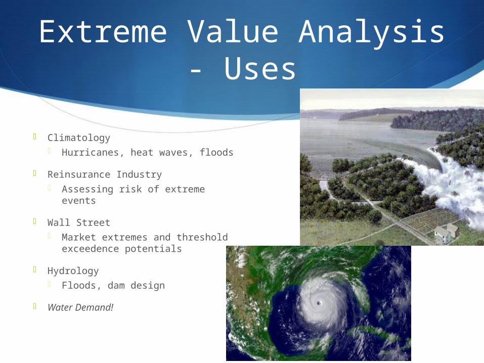
Extreme Value Analysis - Uses
Climatology Hurricanes, heat waves, floods
Reinsurance Industry Assessing risk of extreme events
Wall Street Market extremes and threshold
exceedence potentials
Hydrology Floods, dam design
Water Demand!

Two Approaches To EVA
Block Maxima
location parameter µ scale parameter σ shape parameter k
Used… …in instances where
maximums are plentiful …when user would like
to know the magnitude of an extreme event
Points over Threshold
shape parameter k scale parameter σ threshold parameter θ
Used… …in instances where
data is limited …when user would like
to know with what frequency extreme events will occur
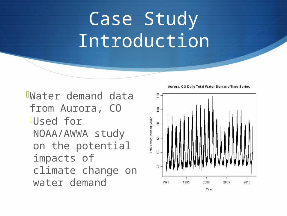
Case Study Introduction
Water demand data from Aurora, CO Used for
NOAA/AWWA study on the potential impacts of climate change on water demand

Generalized Extreme Value Distribution: Block Maxima
Approach‘Block’ or Summer
Seasonal Maxima in Aurora, CO Issues
For water demand data ‘blocks’ could be annual or seasonal
However, this leaves us with a very limited amount of data to fit the GEV with for Aurora
This is not an appropriate method to use because of the limited data

GEV: Block Maxima Approach
Aurora, CO Seasonal Monthly Maximums Compromise
Not a true maxima
However, it allows GEV modeling on smaller data sets
An acceptable approach for GEV modeling

GPD: Points Over Threshold Approach
Daily Water Demand; Aurora, CO Approach
Choose some high threshold
Fit the data above the threshold to a GPD to get intensity of exceedence
Fit the same data to Point Process to get frequency of exceedence

GPD: Points Over Threshold Approach
Capacity of Points Over Threshold Process Uses more data than GEV
Can answer questions like ‘what’s the probability of exceeding a certain threshold in a given time frame?’ or ‘How many exceedences do we anticipate?’
We can also see how return levels will change under given IPCC climate projections
This will give an idea about the impact of climate on water demand

Points Over Threshold
Use The point process fit is a
Poisson distribution that indicates whether or not an exceedence will occur at a given location
The point process fit couples with the GPD fit will be used to model the data

Non-Stationary EVA
Benefits Allows flexible, varying
models
Improved forecasting capacity
Trends in models apparent
Potential covariates Precipitation Temperatures Spell statistics Population Economic forecasts etc
x10

Stationary GEV
Maximum Streamflow (cfs)
PD
F
0 2000 4000 6000 8000
0e+0
01e
-04
2e-0
43e
-04
4e-0
4
Maximum Streamflow (cfs)
PD
F
0 2000 4000 6000 8000
0e+0
01e
-04
2e-0
43e
-04
4e-0
4 Unconditional GEV

Conditional GEV Shifts with Climate Covariates
Maximum Streamflow (cfs)
PD
F
0 2000 4000 6000 8000
0e+0
01e
-04
2e-0
43e
-04
4e-0
4
Maximum Streamflow (cfs)
PD
F
0 2000 4000 6000 8000
0e+0
01e
-04
2e-0
43e
-04
4e-0
4
Maximum Streamflow (cfs)
PD
F
0 2000 4000 6000 8000
0e+0
01e
-04
2e-0
43e
-04
4e-0
4
(Towler et al., 2010)

Maximum Streamflow (cfs)
PD
F
0 2000 4000 6000 8000
0e+0
01e
-04
2e-0
43e
-04
4e-0
4
P[S>Q90Uncond] ??
10%
40%
3%
Q90
Maximum Streamflow (cfs)
0 2000 4000 6000 8000
0e+0
01e
-04
2e-04
3e-04
4e-04
Conditional GEV Shifts with Climate Covariates
(Towler et al., 2010)

Non-Stationary Case
We can allow the extreme value parameters to vary with respect to a variety of covariates
Covariates will be the climate indicators we have been building (temp, precip, PDSI, spells, etc)
Forecasting these covariates with IPCC climate models will give the best forecast of water demand
Climate is non-stationary, water demand fluctuations with respect to climate will also not be stationary
Generalized Parateo Distribution