Extreme Pathway Analysis: Basic Concepts - UCSD...

1

University of California, San DiegoDepartment of Bioengineering

Systems Biology Research Grouphttp://systemsbiology.ucsd.edu

Extreme Pathway Analysis:Basic Concepts

Bernhard PalssonLecture #5

September 15, 2003

2



Outline

• What are pathways?

• Linear basis for Null Space

• Convex basis for the Null Space: Extreme Pathways- Convex analysis- Polyhedral flux cones and pathways

• Types of extreme pathways- Type I- Type II- Type III

• Flux Distributions- Example: Pathway analysis on succinate

A

C E

B

D F

p1

p2

p3

3



Historically defined pathways

• Historically defined pathways include glycolysis and the TCA cycle as shown at the left.

• These pathways are linked reactions which can be grouped together based upon conceptual understanding of a functional role

http://www.accessexcellence.com/AB/GG/glycoCit_prec.html

Historically, “pathways” have been defined as reaction sets linked by having the product of one reaction be the reactant of the next reaction in the chain. These pathways have then been grouped conceptually as functional units such as glycolysis or the TCA cycle. This type of pathway definition is useful for being able to identify portions of the metabolic network, but the divisions are somewhat vague between where one pathway starts and another begins. Also, this type of pathway definition does not relate to the overall functions of the network as a whole.

4



Other figures showing historically defined pathways

Historically defined pathways can be shown in a variety of ways. Examples are shown above.

5



1980

1990

(B.L. Clarke)Stoichiometric Network Analysis developed to study instability in inorganic chemical reaction networks. Relied on kinetic information and utilized concepts of convex analysis.

(A. Seressiotis & J.E. Bailey)Artificial intelligence algorithm developed to search through reaction networks for the identification/synthesis of biochemical pathways

(S. Schuster et.al.)Convex analysis first applied to metabolic networks with the introduction of a non-unique set of elementary modes

(J.C. Liao et.al.)Pathway analysis used to optimize bacterial strain design for high-efficient production of aromatic amino acid precursors

1988

1994

1996

(M.L. Mavrovouniotis et.al.)Stoichiometric constraints used to synthesize pathways again using artificial intelligence searches

The Brief History of Metabolic Pathway Analysis

(C.S. Schilling et.al.)Extreme pathways , the unique and irreducible set of elementary modes, are developed and applied to the study of large scale metabolic networks.

2000

2002(Papin et.al., Price et al.)Extreme pathways are calculated for genome -scale metabolic networks

A BRIEF HISTORY OF THE FIELD OF PATHWAY ANALYSIS.

The first work on pathways can be traced back to 1980 with the development of SNA by Bruce Clarke. The theory was developed to study instability in inorganic chemical networks. This was the first attempt to apply convex analysis to reaction networks but was never extended to living systems. This was followed by some work using AI to search through reaction networks following along the lines of graph theory. This was taken anothe r step by Mavro with the introduction of stoichiometric constraints. Both of these approaches lacked a sound theoretical basis.

In 1994 Schuster became the first to apply convex analysis to me tabolic networks with the introduction of a non-unique set of elementary modes. This theory was applied a few years later by Liao to optimize bacterial strain design for the high-efficient production of aromatic amino acids.

So at this point in time pathway analysis is just beginning to be applied but still lacks a unified theoretical foundation, which is where the present work comes in.

6



Linear basis for Null space

7



The Null Space of the Stoichiometric Matrix

• Contains all the solutions to Sv=0• These are the steady state solutions to the dynamic mass balances• The time constants of metabolic transients are typically very fast, i.e.

shorter than about 1 to 5 minutes, especially in bacteria• Thus for most practical purposes metabolism is in a steady state• The null space contains all the steady state flux distributions and is

thus of special importance to us

• The dimension of the null space is the number of columns in the matrix minus the number of independent rows (the rank of the matrix)

Metabolic Transients and the Null Space

The concentrations of metabolites tend to be very low, on the order of micro-molar, or about 60,000 molecules per E. coli cell. Yet the metabolic fluxes are about 100,000 molecules per sec per cell. Thus, the average response time of a metabolic concentration is about 1 second. These transients are too fast for essentially all practical purposes.

Metabolites that are in higher concentrations, such as ATP, can have time constants that are on the order of minutes. Nevertheless, compared to the progression of an infection or bioprocessing, this time is very short and metabolism is very fast, and can be effectively considered to be in a steady-state.

In some highly specialized mammalian cells, metabolic transients can be slower. For instance, in the human red blood cell, the ATP turnover time is about a hour, and transient changes in 2,3DPG are on a 12 to 24 hr time scale. 2,3DPG binds to hemoglobin to regulate its affinity for oxygen. This time constant is responsible for the time that it takes us to adjust to higher altitudes.

8



Finding the basis for the null space

Any matrix A:

Can be row reduced using Gaussian elimination:

Finding a Basis for the Null Space

A basis for the null space can be found by a so-called parameterization procedure. First any matrix A is row-reduced by Gaussian elimination into the echelon form of the matrix (typically denoted by U). The pivot columns are identified (columns one and three in the example given). These are the columns with the pseudo-diagonal elements. These columns represent the fixed variables. The free variables are in the columns between the pivot columns (the second, fourth and fifth in the example given).

9



The matrix A has two pivot columns (1 and 3) and three free variables (2,4,5). All the variables can be expressed in terms of the free variables (parametric form)

Then the vectors u, v, w span the 3-dimensional null space

Finding a Basis for the Null Space--continued

All the variables are then written in terms of the free variables. The equations are then written in vector form by factoring out the free variables individually. The columns that form constitute a spanning set--a basis--for the null space of A. The free variables can take on any numerical values to form additions of these basis vectors.

Verify that Au=Av=Aw=0, and that u,v,w is an independent set of vectors.

10



1 −1 0 0 −1 0

0 1 −1 0 0 00 0 1 −1 0 1

0 0 0 0 1 −1

v1

v2

v3

v4

v5

v6

=

0

00

0

0

00

0

65

643

32

521

=−=+−

=−=−−

vvvvv

vvvvv

Flux balancesStoichiometric Matrix

S• v= 0

General Solution

v1

v2

v3

v4

v5

v6

=

v4

v4 − v6

v4 − v6

v4

v6

v6

= v4

111100

+v6

0−1−1011

= v4b1 + v6b2

Nul S = Span b1, ...,bi{ }= v : v = wibi∑ , ∀ i

A

B

D

C

b1

b2

Basis vectors mapped onto the network

A

B

D

Cv1

v2 v3v4

v5 v6

Reaction network

Finding a Basis for an Example Stoichiometric Matrix

A simple reaction network is presented in the ULH panel. The corresponding stoichiometric matrix and its flux balances are written in the URH panel. The parameterization method of the previous two slides is applied to find a basis for this stoichiometric matrix, as shown in the LLH panel. These basis vectors can be graphically represented on the metabolic map (LRH Panel).

Note that the two basis vectors form a string of connected reactions--effectively pathways. The first basis vector, b1, is a straight through pathway through the upper part of this small network. The second basis vector, b2, is a circular path. It has steps in it that run opposite to the direction of two irreversible reactions. Although the basis vectors form mathematically acceptable pathways, they are not biochemically acceptable. However, as we saw previously, we can form another equivalent basis.

11



Particular Solution

v =

211211

= w1b1 + w2b2 = (2)

111100

+(1)

0−1−1011

=(2)b1 +(1)b2 A

B

D

C(1)*b2

Flux distribution decomposed into pathways

2 211

1 1

Basis Transformation

P = p1,p2{ }=p1 = b1

p2 =b1 +b2

TB→P =1 10 1

B PB• TB→P = P

B•T=

1 01 −11 −11 00 10 1

1 10 1

=

1 11 01 01 10 10 1

=P p1,p2{ }A

B

D

C

Basis vectors as biochemical pathways

p1

p2

Finding a Basis for an Example Stoichiometric Matrix--continued

Every flux distribution, v, can be uniquely described by a combination of the particular set of basis vectors chosen to describe the null space, (Unique Representation Theorem). An example is given in the ULH panel and shown on the metabolic map in the URH panel.

A basis for a vector space imposes a coordinate system on the space. However, this coordinate system is not unique, which implies that other sets of vectors can be used as a basis for the same vector space. One basis can be transformed into another using a basis transformation, as shown in the LLH panel. We seek to find basis vectors whose elements are all positive. Such vectors will form biochemically acceptable pathways as shown in the LRH panel.

12



1 −1 0 −1 0 0 0 0 0

0 1 −1 0 0 0 0 0 10 0 0 1 −1 −1 0 0 0

0 0 0 0 1 0 −1 0 00 0 0 0 0 1 0 1 −10 0 0 0 0 0 1 −1 0

v1

v2

v3

v4

v5

v6

v7

v8

v9

=

0

00

000

Stoichiometric Matrix

General Solution (free variables v3, v8, v9)

v1

v2

v3

v4

v5

v6

v7

v8

v9

=

v3

v3 − v9

v3

v9

v8

v9 − v8

v8

v8

v9

= v3

111000000

+v8

00001−1110

+ v9

0−10101001

= v3b1 + v8b2 + v9b3

Metabolic Network (Example #2)

A

C E

Bv1 v2

v9v4

v5

v6

D F

v3

v7

v8

Basis vectors mapped onto the network

A

C E

B

D F

b1

b2

b3

Note b2 and b3 violate reaction thermodynamics

Finding a Basis for a Stoichiometric Matrix

EXAMPLE #2

Here is another example of a reaction network in which two of the basis vectors form mathematically acceptable pathways, but not biochemically acceptable pathways.

13



Basis Transformation (Example #2)

P = p1,p2,p3{ }=p1 = b1

p2 =b1 +b2 + b3

p3 =b1 +b3

TB→P =

1 1 1

0 1 00 1 1

B PB• TB→ P = P

B•T=

1 0 01 0 −11 0 00 0 10 1 00 −1 10 1 00 1 00 0 1

1 1 10 1 00 1 1

=

1 1 11 0 01 1 10 1 10 1 00 0 10 1 00 1 00 1 1

= P p1,p2,p3{ }

Basis vectors as biochemical pathways

A

C E

B

D F

p1

p2

p3

The selection of basis vectors is not unique. Therefore it is irrelevant that any flux distribution can be uniquely represented by a set of basis vectors. We need to try and find a unique “basis” or set of pathways to describe the solution space.

All of the pathways now obey the thermodynamic constraints if they are positively weighted.

Finding a Basis for a Stoichiometric Matrix

EXAMPLE #2--CONTINUED

Again, through a basis transformation, we find three biochemically acceptable pathways.

14



Convex basis for the Null Space:Extreme Pathways

15



Convex Analysis

• The study of systems of linear equations and inequalities

• Convex analysis is used to study metabolic networks where the linear equations are derived from the mass balances and the inequalities are generated from thermodynamic information on the reversibility of reactions.

• From linear algebra a null space is defined which contains all of the solutions to the set of linear homogenous equations. When we add inequality constraints (such as all variables must be positive) the solution space becomes restricted by these inequalities (the portion of the null space in the positive orthant)

Convex Analysis•Convex analysis is used to study metabolic networks where the linear equations are derived from the mass balances and the inequalities are generated from thermodynamic information on the reversibility of reactions.•From linear algebra a null space is defined which contains all of the solutions to the set of linear homogenous equations. When we add inequality constraints (such as all variables must be positive) the solution space becomes restricted by these inequalities (the portion of the null space in the positive orthant)

16



What is Convexity?Definition of a Convex Space: For every two points in the space, the line connecting these two points lies entirely withinthe space.

Convex Shapes Non-Convex Shapes

What is Convexity?Definition of a Convex Space: For every two points in the space, the line connecting these two points lies entirely within the space.

17



Extreme pathways capture the phenotypic potential of metabolic reaction networks

flux vA

flux

v Bflu

x v C

Reaction Network Model

Pathway Analysis

Phenotypic Potential of the Reaction Network

Creation of Stoichiometric Matrix

− 01..2

00........

...10

1..01 Metabolites

Reactions

Extreme pathways have the following characteristics:

1) They are a unique and minimal set of basis vectors

2) All possible phenotypes can be represented by non-negative linear combinations of the EPs

3) They represent time-invariant properties of the metabolic network

18



Polyhedral Cones and Pathways

• Region determined by a linear homogeneous equation/inequality system is a convex polyhedral cone (C)

• Every point in the cone is a non-negative combination of the generating vectors (Extreme Pathways) of the cone

• The number of generating vectors can exceed the dimensions of the cone (i.e. linearly dependent)

• Generating vectors represent systemically independentpathways which can theoretically be“switched” on or off

• Generating vectors are unique for a system

C= v ∈Rn v= αipi , αi ≥ 0

i=1

k∑

0 = S• v, vi ≥ 0, i =1,...,n p1

p5

p4

p3

p2

THE FLUX CONES

Through the principles of convex analysis it turns out that the shape of the null space for a set of linear equation with positive flux values such as the systems which we are concerned with is a convex polyhedral cone such as the one depicted here on the right. The perspective of the cone is supposed to look as if it is going into the plane of the slide. What is nice about cones is the condition that every point within the cone can be described as a non-negative combination of the generating vectors where the generating vectors are the edges of the cone. If we can determine these generating vectors which are biochemically feasible, then we can describe every point within the cone. Additionally the number of generating vectors can exceed the dimensions of the cone which has the mathematical consequence that all of these pathways are not linearly independent. The best analogy for some of these concepts is to think of an Egyptian pyramid which has 4 edges and exists in three dimensional space. Algorithms exist for the determination of these generating vectors and the set of generating vectors represents what may be referred to as genetically independent pathways. This means that each pathway utilizes a unique set of reactions and gene products utilizing a different genotype. Also extremely important is the fact that the set of generating vectors is unique. So, to best describe the null space and navigate through the metabolic map of an organism, we have to determine this unique set of genetically independent pathways.

19



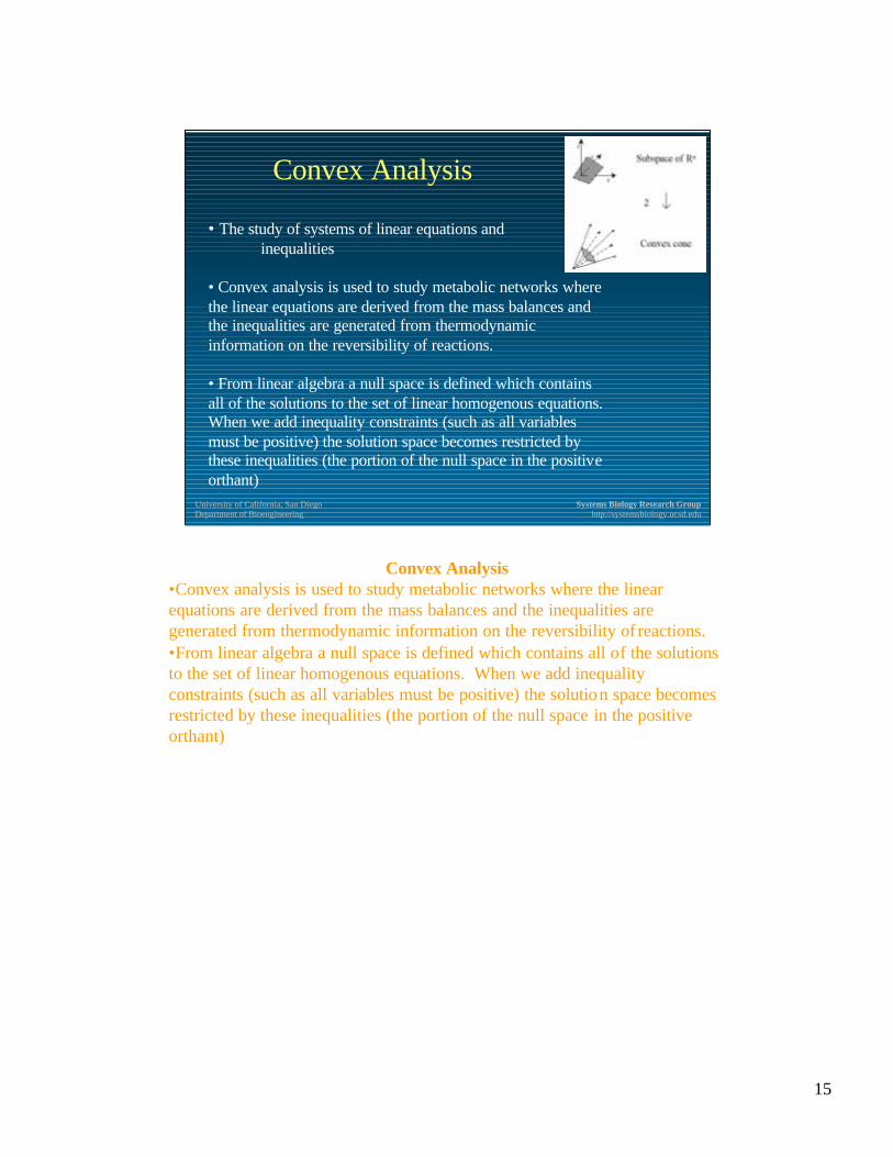
Metabolic Genotype & PhenotypeDefined within the context of convex analysis

Convex AnalysisConvex Analysis Cellular BiologyCellular Biology

Unique GeneratingVectors

IndependentExtreme Pathways

Flux VectorPositive Combination of Extreme Pathways

met

abol

ic fl

ux (

v 1)

metabolic flux (

v2 )

metabolic flux (

v3)

Convex HullCapabilities of a Metabolic Genotype

Particular SolutionMetabolic Phenotype

C= v ∈Rn v = αipi, αi ≥ 0

i=1

k∑

NIFTY INTERPRETATION OF THE FLUX CONE

So what does this all mean from a biological point of view. Here is the geometric interpretation of the flux cone in which every point is described by the equation given. The entire flux cone actually corresponds to the capabilities of a reaction network and hence the defined metabolic genotype. What can the reconstructed network do, what can it not do? Each one of the generating vectors corresponds to an extreme pathway which the cell could theoretically control to reach every point in the flux cone. Now a particular point within this flux cone corresponds to a given flux distribution which represents a particular metabolic phenotype. The actual flux vector describing that point can be thought of as a positive combination of these extreme pathways. So you may think of these pathways as being theoretically turned on and off to reach a particular metabolic phenotype. Once again this means that every phenotype which the system can exhibit is a combination of these pathways which are then turned on or off. It’s that simple. With these pathways we can describe all of the capabilities of the metabolic system, and so we may say that these pathways represent the underlying pathway structure of the system.

20



Extreme PathwaysA B C

D

E

v → Internal Fluxb → Exchange Flux

System Boundary

b1

b2

b3

b4

v1 v2

v3

v4 v5

v6

v7

Biochemical Reaction Network

7 internal fluxes+ 4 exchange fluxes

n = 11 fluxesm = 5 metabolites

• stoichiometric matrix (5 x 11)• dimension of null space = 6• # of extreme pathways = 8

A B C

p3

B

Dp8

B C

Dp7

A B C

D

E

p6

A B C E

p1

A B

D

p2

A B C

D

p5

A B

D

E

p4

WHAT DO THE EXTREME PATHWAYS LOOK LIKE?

Here is an example of what extreme pathways look like for the hypothetical reaction network shown above. In this case the stoichiometric matrix is 5 by 11 with the dimensions of the null space equaling 6 and the number of extreme pathways equaling 8. We can see here that 6 of these pathways are actually performing net reactions which consume a metabolite to produce another, however there are two pathways here that are only internal cycles within the network. So we see the necessity for a classification scheme for these pathways.

Compare these pathways to the linked output pathways that appear on a later slide.

21



Linear Spaces

Described by linear equations

Vector spaces defined by a set of linearly independent basis vectors (bi)

Every point in the vector space is uniquely described by a linear combination of basis vectors (unique representation for a given basis)

Number of basis vectors equals dimension of the null space

Infinite number of bases that can be used to span the space

v = wibi − ∞≤wi ≤ +∞∑

Convex Spaces

Described by linear equations and inequalities

Convex polyhedral cone defined by a set of conically independent generating vectors (pi)

Every point in the vector space is described as a non-negative linear combination of the generating vectors (non-unique representation)

Number of generating vectors equals edges of the polyhedral cone and may exceed dimensions of the null space

Unique set of generating vectors.

v = wipi 0 ≤wi ≤ +∞∑

COMPARING LINEAR SPACES AND CONVEX ANALYSIS

The number of generating vectors can exceed the dimensions of the cone which has the mathematical consequence that all of these pathways are not linearly independent. While not linearly independent, these pathways are systemically independent in that they cannot be decomposed into a combination of other pathways in a convex manner. An important fact is that the set of generating vectors is unique and below we represent algorithms to solve for these generating vectors. Thus, to describe the flux space and navigate through the metabolic map of an organism we have to determine that it is best to use this unique set of systemically independent pathways.

This set of pathways can be thought of as the “operating system” for a defined metabolic genotype, since the control over these pathways will enable the attainment of any state (phenotype) allowable by the constraints placed on the metabolic system.

22



Types of Extreme Pathways

23



Classifying Pathways• Type I: Primary Metabolic Pathways• Type II: “Futile” Cycles

– only currency exchange fluxes active

• Type III: Reaction Cycling – no active exchange fluxes

Type I Type II

Type III

Cofactor pools

Cofactor pools

Cofactor pools

Substrates

Products

Classifying Extreme Pathways

Extreme pathways can be categorized into three types, based upon their exchange fluxes.

Type I extreme pathways have exchange fluxes that cross system boundaries, and represent primary metabolic pathways. These extreme pathways detail the conversion of substrates into products and byproducts.

Type II extreme pathways also have exchange fluxes that cross system boundaries, but these exchange fluxes only correspond to “currency” metabolites, such as ATP, NADH and so forth. Type II pathways can be through of as “futile” cycles, and must proceed “downhill” in terms of free energy.

Type III extreme pathways have no active exchange fluxes, and therefore represent internal cycles. Based upon thermodynamics, these cycles cannot be active because there is no energy source to drive them. Thus, these type III extreme pathways can be eliminated from the convex basis without loss of phenotypic potential.

24



hk

pgi

pfk

ald

gapdh

tpi

tpgk

pgl

dpgppgm

en

ldh

pk

dpgm

g6pdh pgdh

rpixpi

ta

tkI

tkII

b1

b2

b3

b4

b5

Red Blood Cell Metabolic Network

2,3DPG

DHAP

F6P

G6P

FDP

GA3P

D6PGC RL5PD6PGL

R5PX5PF6P

S7P

E4P

GLC

GA3P

GA3P

F6P

3PG

2PG

PEP

PYR

LAC

1,3-DPG

ATP

ADP

NAD

NADH

NADP

NADPH

Pi

CO2

b6

b8

b7

b11

b9

b10

b12

b13

Pathway Classification: Type IPrimary Metabolic Pathways

hk

pgi

pfk

ald

gapdh

tpi

tpgk

pgl

dpgppgm

en

ldh

pk

dpgm

g6pdh pgdh

rpixpi

ta

tkI

tkII

b1

b2

b3

b4

b5


2,3DPG

DHAP

F6P

G6P

FDP

GA3P

D6PGC RL5PD6PGL

R5PX5PF6P

S7P

E4P

GLC

GA3P

GA3P

F6P

3PG

2PG

PEP

PYR

LAC

1,3-DPG

ATP

ADP

NAD

NADH

NADP

NADPH

P i

CO2

b6

b8

b7

b11

b9

b10

b12

b13

Glucose conversion to Pyruvate Glucose conversion to 2,3-DPG

TYPE I PATHWAYS

The first type of pathways that are generated are what we refer to as primary pathways and these are the types of pathways that first come to mind when thinking about a metabolic map. These are simply pathways that connect an input to an output. The only requirement of the pathway is that one of the primary exchange fluxes must be active. Here are two examples of primary metabolic pathways that are extreme pathways on the cone. The green arrow denote the production of a metabolite by the pathway and the red arrows indicate the consumption of a metabolite while the white arrows indicate the internal fluxes which are operating.

The first example is simply the conversion of glucose to pyruvate using the glycolytic pathway . This is basically the glycolytic pathway that picks up glucose and secretes pyruvate, and produces both ATP and NADH.

The second pathway is the production of 2,3DPG from the Rapoport-Luebering shunt. This pathway becomes active when more 2,3DPG needs to be produced, such as when one goes through changes in altitude and the oxygen binding characteristics of hemoglobin need to be changes. This will always be a low flux pathway.

25



Pathway Classification: Type II“Futile” Cycles - (only currency exchange fluxes active)

Dissipation of ATP

hk

pgi

pfk

ald

gapdh

tpi

tpgk

pgl

dpgppgm

en

ldh

pk

dpgm

g6pdh pgdh

rpixpi

ta

tkI

tkII

b1

b2

b3

b4

b5


2,3DPG

DHAP

F6P

G6P

FDP

GA3P

D6PGC RL5PD6PGL

R5PX5PF6P

S7P

E4P

GLC

GA3P

GA3P

F6P

3PG

2PG

PEP

PYR

LAC

1,3-DPG

ATP

ADP

NAD

NADH

NADP

NADPH

Pi

CO2

b6

b8

b7

b11

b9

b10

b12

b13

TYPE II PATHWAYS

The second type of pathway is what is commonly referred to as a futile cycle in the truest sense of the word futile. In these pathways only the exchange fluxes for the currency metabolites are active. In this system there exists one futile cycle which occurs around the Rapoport-Luebering shunt. The net result of this pathway is the conversion of ATP into ADP and releasing inorganic phosphate which is obviously dissipating metabolic energy.

There is one futile cycle that operates in this system.

26



Pathway Classification: Type IIIReaction Cycling - (no active exchange fluxes)

16 Reversible Reactions

hk

pgi

pfk

ald

gapdh

tpi

tpgk

pgl

dpgppgm

en

ldh

pk

dpgm

g6pdh pgdh

rpixpi

ta

tkItkII

b1

b2

b3

b4

b5


2,3DPG

DHAP

F6P

G6P

FDP

GA3P

D6PGC RL5PD6PGL

R5PX5PF6P

S7P

E4P

GLC

GA3P

GA3P

F6P

3PG

2PG

PEP

PYR

LAC

1,3-DPG

ATP

ADP

NAD

NADH

NADP

NADPH

Pi

CO2

b6

b8

b7

b11

b9

b10

b12

b13

TYPE III PATHWAYS

The third type of pathway consists of reversible cycles which are mainly the result of reversible reactions that can be characterized by a forward reaction and a separate reverse reaction. These pathways show no activity in any of the exchange fluxes. In this map all 16 reversible reactions are highlighted white. While these pathways are essentially generating vectors they can effectively be dismissed in any further analysis of the system as they have no net effect on the production capabilities of the system as they influence none of the exchange fluxes.

These pathways will become important later when we examine temporal decomposition of this system. A fast internal pathway leads to an ‘equilibration’ or the ‘tying together’ of two or more concentrations that then can be ‘pooled’ together to form an aggregate dynamic variable. Some simple examples of this feature were show in the last lecture.

Together all of the extreme pathways in a system fall under one of these three classifications of pathways and they all are edges of the cone determining the flux space.

27



Linked Outputs

28



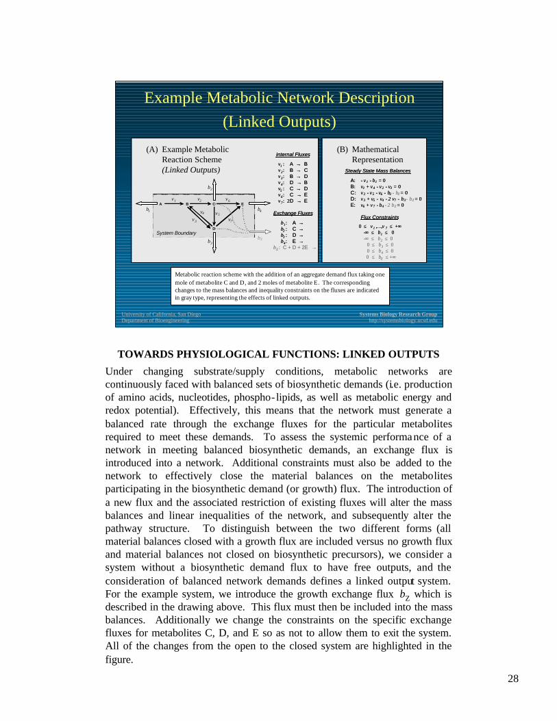
Example Metabolic Network Description (Linked Outputs)

A B C

D

E

System Boundary

b1

b2

b3

b4

v1 v2

v3

v4 v5

v6

v7

Internal Fluxes

v1 : A → Bv2 : B → Cv3 : B → Dv4 : D → Bv5 : C → Dv6 : C → Ev7 : 2D → E

Exchange Fluxes

b1 : A →b2 : C →b3 : D →b4 : E →

bZ : C + D + 2E →

Internal Fluxes

v1 : A → Bv2 : B → Cv3 : B → Dv4 : D → Bv5 : C → Dv6 : C → Ev7 : 2D → E

Exchange Fluxes

b1 : A →b2 : C →b3 : D →b4 : E →

bZ : C + D + 2E →

(A) Example Metabolic Reaction Scheme (Linked Outputs)

(B) Mathematical Representation

Steady State Mass Balances

A: - v1 - b1 = 0B: v1 + v4 - v2 - v3 = 0C: v2 - v5 - v6 - b2 - bZ = 0D: v3 + v5 - v4 - 2 v7 - b3 - bZ = 0E: v6 + v7 - b4 - 2 bZ = 0

Flux Constraints

0 ≤ v1 ,…,v 7 ≤ +∞-∞ ≤ b1 ≤ 0 -∞ ≤ b2 ≤ 0

0 ≤ b3 ≤ 0 0 ≤ b4 ≤ 0 0 ≤ bZ ≤ +∞

Steady State Mass Balances

A: - v1 - b1 = 0B: v1 + v4 - v2 - v3 = 0C: v2 - v5 - v6 - b2 - bZ = 0D: v3 + v5 - v4 - 2 v7 - b3 - bZ = 0E: v6 + v7 - b4 - 2 bZ = 0

Flux Constraints

0 ≤ v1 ,…,v 7 ≤ +∞-∞ ≤ b1 ≤ 0 -∞ ≤ b2 ≤ 0

0 ≤ b3 ≤ 0 0 ≤ b4 ≤ 0 0 ≤ bZ ≤ +∞

bZ

Metabolic reaction scheme with the addition of an aggregate demand flux taking one mole of metabolite C and D, and 2 moles of metabolite E. The corresponding changes to the mass balances and inequality constraints on the fluxes are indicated in gray type, representing the effects of linked outputs.

TOWARDS PHYSIOLOGICAL FUNCTIONS: LINKED OUTPUTS

Under changing substrate/supply conditions, metabolic networks are continuously faced with balanced sets of biosynthetic demands (i.e. production of amino acids, nucleotides, phospho- lipids, as well as metabolic energy and redox potential). Effectively, this means that the network must generate a balanced rate through the exchange fluxes for the particular metabolites required to meet these demands. To assess the systemic performance of a network in meeting balanced biosynthetic demands, an exchange flux is introduced into a network. Additional constraints must also be added to the network to effectively close the material balances on the metabolites participating in the biosynthetic demand (or growth) flux. The introduction of a new flux and the associated restriction of existing fluxes will alter the mass balances and linear inequalities of the network, and subsequently alter the pathway structure. To distinguish between the two different forms (all material balances closed with a growth flux are included versus no growth flux and material balances not closed on biosynthetic precursors), we consider a system without a biosynthetic demand flux to have free outputs, and the consideration of balanced network demands defines a linked output system. For the example system, we introduce the growth exchange flux bZ which is described in the drawing above. This flux must then be included into the mass balances. Additionally we change the constraints on the specific exchange fluxes for metabolites C, D, and E so as not to allow them to exit the system. All of the changes from the open to the closed system are highlighted in the figure.

29



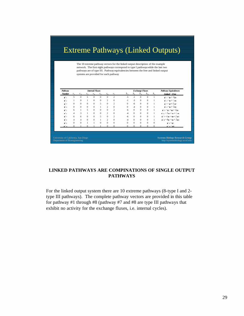
Extreme Pathways (Linked Outputs)

Pathway Equivalencesv1 v 2 v3 v4 v5 v6 v7 b 1 b2 b 3 b 4 b z Linked ~ Free

p' 1 5 0 5 0 0 0 2 -5 -1 0 0 1 p' 1 ~ p2 + 2 p3

p' 2 1 0 1 0 0 2 0 -1 -3 0 0 1 p' 2 ~ p2 + 2 p6

p' 3 0 0 0 0 5 0 2 0 -6 0 0 1 p' 3 ~ p4 + 2 p5

p' 4 0 0 0 0 1 2 0 0 -4 0 0 1 p' 4 ~ p4 + 2 p6

p' 5 6 1 5 0 0 0 2 -6 0 0 0 1 p' 5 ~ p1 + p2 + 2 p3

p' 6 4 3 1 0 0 2 0 -4 0 0 0 1 p' 6 ~ 3 p1 + p2 + 2 p6

p' 7 6 6 0 0 5 0 2 -6 0 0 0 1 p' 7 ~ 6 p1 + p4 + 2 p5

p' 8 4 4 0 0 1 2 0 -4 0 0 0 1 p' 8 ~ 4 p1 + p4 + 2 p6

p' 9 0 0 1 1 0 0 0 0 0 0 0 0 p' 9 ~ p7

p' 10 0 1 0 1 1 0 0 0 0 0 0 0 p' 10 ~ p8

Pathway Number

Internal Fluxes Exchange Fluxes

The 10 extreme pathway vectors for the linked output description of the example network. The first eight pathways correspond to type I pathways while the last two pathways are of type III. Pathway equivalencies between the free and linked output systems are provided for each pathway

LINKED PATHWAYS ARE COMPINATIONS OF SINGLE OUTPUT PATHWAYS

For the linked output system there are 10 extreme pathways (8-type I and 2-type III pathways). The complete pathway vectors are provided in this table for pathway #1 through #8 (pathway #7 and #8 are type III pathways that exhibit no activity for the exchange fluxes, i.e. internal cycles).

30



A B C

D

E

p’1

-5

5

52

1

-1

A B C

D

E

p’1

-5

5

52

1

-1

A B C

D

E

p’2

-1

-3

1

1

2

1

A B C

D

E

p’2

-1

-3

1

1

2

1

A B C

D

E

p’3

-6

5 2

1

A B C

D

E

p’3

-6

5 2

1

A B C

D

E

p’4

-4

1

2

1

A B C

D

E

p’4

-4

1

2

1

A B C

D

E

p’5

-6

6 1

52

1

A B C

D

E

p’5

-6

6 1

52

1

A B C

D

E

p’6

-4

4 3

1

2

1

A B C

D

E

p’6

-4

4 3

1

2

1

A B C

D

E

p’7

-6

6 6

5 2

1

A B C

D

E

p’7

-6

6 6

5 2

1

A B C

D

E

p’8

-4

4 4

1

2

1

A B C

D

E

p’8

-4

4 4

1

2

1

Linked Pathways

and

FluxDistributions

GRAPHICAL REPRESENTATION OF LINKED PATHWAYS

The pathway distributions are also illustrated graphically in this figure. Note that the extreme pathways for the linked outputs are systemic flux distributions that meet the balanced set of demands represented by the growth flux (bz). These extreme pathways are non-negative combinations of the extreme pathways for the free output system. This leads to the definition of pathway equivalences that relate the free output system pathways to the linked output system.

The first two produce the required output using two inputs (A and C), the next two only from C, and the last four from A alone.

Compare these to the single output pathways shown on an earlier slide for the same network.

The linked pathways are no longer ‘linear’ or ‘one-dimensional’ entities, but actual flux maps.

31



Flux Distributions

32



E4PX5PGLCxt

G6P

F6P

FDP

DHAP

3PG

DPG

GA3P

2PG

PEP

PYR

AcCoA

SuccCoA

SUCC

AKG

ICIT

CIT

FUM

MAL

OAA

Ru5P

R5P

S7P

6PGA 6PG

ACTP

ETH

ATP

NADPHNADH FADH

Qh2+H

SUCCxt

pts

pts

pgi

pfkA

fba

tpi

fbp

gapA

pgk

gpmA

eno

pykFppsA

aceE

zwfpgl gnd

rpiA

rpe

talAtktA1 tktA2

gltA

acnA icdA

sucA

sucC

sdhA1

frdA

fumA

mdh

adhE

AC

ackA

pta

pckA

ppc

cyoA

pntA

sdhA2nuoA

atpA

ACxt

ETHxt

O2 O2xt

CO2 CO2xt

Pi Pixt

O2 trx

CO2 trx

Pi trx

EXTRACELLULARMETABOLITE

reaction/gene name

Map Legend

INTRACELLULARMETABOLITE

GROWTH/BIOMASSPRECURSORS

ETH trx

AC trx

SUCC trx

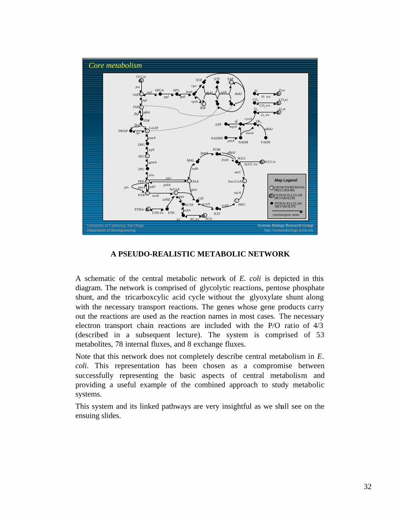
Core metabolism

A PSEUDO-REALISTIC METABOLIC NETWORK

A schematic of the central metabolic network of E. coli is depicted in this diagram. The network is comprised of glycolytic reactions, pentose phosphate shunt, and the tricarboxcylic acid cycle without the glyoxylate shunt along with the necessary transport reactions. The genes whose gene products carry out the reactions are used as the reaction names in most cases. The necessary electron transport chain reactions are included with the P/O ratio of 4/3 (described in a subsequent lecture). The system is comprised of 53 metabolites, 78 internal fluxes, and 8 exchange fluxes.

Note that this network does not completely describe central metabolism in E. coli. This representation has been chosen as a compromise between successfully representing the basic aspects of central metabolism and providing a useful example of the combined approach to study metabolic systems.

This system and its linked pathways are very insightful as we shall see on the ensuing slides.

33



SUCCxt/ SUCCxt

ETHxt/ SUCCxt

ACxt/ SUCCxt

GRO/ SUCCxt

PIxt/ SUCCxt

CO2xt/ SUCCxt

O2xt/ SUCCxt

1 -1.000 0 0 0.051 -0.188 1.825 -1.267

10 -1.000 0 0 0.049 -0.182 1.895 -1.338

20 -1.000 0 0 0.047 -0.172 1.696 -1.142

3 -1.000 0 0.000 0.034 -0.125 2.553 -2.014

7 -1.000 0 0.000 0.033 -0.121 2.600 -2.062

12 -1.000 0 0 0.032 -0.117 2.644 -2.108

16 -1.000 0.000 0 0.031 -0.114 2.679 -2.144

19 -1.000 1 0.000 0.025 -0.092 1.837 -0.759

23 -1.000 0.000 0.000 0.000 0.000 4.000 -3.500

27 -1.000 0.000 1 0.000 0.000 2.000 -1.500

31 -1.000 1.000 0 0.000 0.000 2.000 -0.500

35 -1.000 0.000 0 0.000 0.000 4.000 -3.500

SUCCxt + 1.5 O2xt Þ 2.0 CO2xt + 1.0 ACxt SUCCxt + 0.5 O2xt Þ 2.0 CO2xt + 1.0 ETHxt

SUCCxt + 3.5 O2xt Þ 4.0 CO2xt

SUCCxt + 0.117 PIxt + 2.108 O2xt Þ 0.032 GRO + 2.644 CO2xt SUCCxt + 0.114 PIxt + 2.144 O2xt Þ 0.031 GRO + 2.679 CO2xt SUCCxt + 0.092 PIxt + 0.759 O2xt Þ 0.025 GRO + 1.837 CO2xt + 0.549 ETHxt SUCCxt + 3.5 O2xt Þ 4.0 CO2xt

SUCCxt + 0.182 PIxt + 1.338 O2xt Þ 0.049 GRO + 1.895 CO2xt SUCCxt + 0.172 PIxt + 1.142 O2xt Þ 0.047 GRO + 1.696 CO2xt + 0.158 ACxt SUCCxt + 0.125 PIxt + 2.014 O2xt Þ 0.034 GRO + 2.553 CO2xt SUCCxt + 0.121 PIxt + 2.062 O2xt Þ 0.033 GRO + 2.6 CO2xt

Pathway Number

Exchange FluxesNet Pathway Reaction Balance

SUCCxt + 0.188 PIxt + 1.267 O2xt Þ 0.051 GRO + 1.825 CO2xt

Functional characteristics of the reduced set of 12 extreme pathways calculated for succinate as the sole carbon source for the E. coli metabolic network with linked outputs. Pathways are ordered based on the activity of the growth flux normalized by the succinate uptake. Pathway numbers coincide with the original numbers of the pathway vectors retained from the complete set. All of the exchange flux values are normalized to the succinate intake level (negative values are relative uptake ratios, positive values are production ratios). Exchange flux abbreviations: SUCC-succinate, ETH-ethanol, AC-acetate, PI-inorganic phosphate, CO2-carbon dioxide, O2-oxygen, GRO-biomass/growth flux .

PATHWAYS FOR GROWTH ON SUCCINATE

The pathway analysis was performed with succinate as the sole carbon source for the system, generating the complete set of 66 extreme pathways (36 type I and 30 type III). To generate a reduced set of pathways that represents the full capabilities of the network, we retain only pathways from these sets that utilized the ATP drain flux instead of one of the three futile cycles; i.e. (pfkA/fbp), (pckA, ppc), (pykF,ppsA,adk). The type III pathways, which are mainly a consequence of the decomposition of reversible reactions into a forward and a reverse reaction, are also removed from consideration as they show no activity in the exchange fluxes. Following this simplification, a reduced set of 12 pathways is generated from the complete set.

The pathways in the table are ordered by the biomass yield that they generate (mg/mol Succinate). The best pathway produces 0.051 biomass units. This represents the optimal use of the network to produce biomass. Note that the next-best pathway produces 0.049 and is in general very similar to the best one. This is a feature that one observes. There are ‘bundles’ of extreme pathways located ‘close’ in this high dimensional conical space, which biologically is a reflection of the redundancy of the system.

The third pathway represents partially aerobic growth and the secretion of acetate. As we shall see later, if oxygen is limiting, then the growth becomes a combination of this pathway and pathway #1. Note that there are two purely fermentative pathways producing acetate and ethanol respectively.

34



E4PX5PGLCxt

G6P

F6P

FDP

DHAP

3PG

DPG

GA3P

2PG

PEP

PYR

AcCoA

SuccCoA

SUCC

AKG

ICIT

CIT

FUM

MAL

OAA

Ru5P

R5P

S7P

6PGA 6PG

ACTP

ETH

ATP

NADPHNADH FADH

Qh2+H

SUCCxt

AC ACxt

ETHxt

O2 O2xt

CO2 CO2xt

Pi Pixt

0.40

0.18

0.18

0.18

0.27

0.27

0.35

0.35

0.48

0.34

0.39

0.39 0.390.17

0.22

0.120.120.10

0.15

0.15 0.15

0.09

0.09

1.091.09

1.09

0.85

1.09

1.44

2.65

1.27

1.83

0.19

1.00

Biomass Yield

0.051 g DW / mmole SUCCor

0.432 g DW / g SUCC

Succinateoptimal fluxdistribution

1.27

Succinate optimal flux distribution

THE OPTIMAL PATHWAY (FLUX MAP)

Flux balance analysis can be used to quantitatively examine the system with linked outputs. Geometrically, the constraints imposed on the input values of the exchange fluxes will bound the flux cone by the extreme pathways into a bounded polyhedron. Optimal solutions within this space will then lie on a vertex of the polyhedron. These are the bounded feasible solutions of the linear programming problem.

The flux distributions for growth are calculated on succinate normalized to 1 mmol of substrate. The optimal flux distributions are illustrated in this figure. The optimal biomass yield is 0.051 g DW/mmol succinate, which is identical to the optimal yield calculated from the pathways (pathway #1). This result reveals that the optimal solution lies directly on the vertex of the polyhedron that is defined by the extreme pathway.

35



E4PX5PGLCxt

G6P

F6P

FDP

DHAP

3PG

DPG

GA3P

2PG

PEP

PYR

AcCoA

SuccCoA

SUCC

AKG

ICIT

CIT

FUM

MAL

OAA

Ru5P

R5P

S7P

6PGA 6PG

ACTP

ETH

ATP

NADPHNADH FADH

Qh 2+H

SUCCxt

AC ACxt

ETHxt

O2 O2xt

CO2 CO2xt

Pi Pixt

0.76

0.30

0.30

0.30

0.38

0.38

0.46

0.46

0.37

0.24

0.75

0.75 0.750.29

0.46

0.240.240.22

0.05

0.05 0.05

1.001.00

1.00

0.86

1.00

1.68

2.90

1.34

1.89

0.18

1.00

Biomass Yield


0.415 g DW / g SUCC

Succinate 2nd

optimal fluxdistribution

0.65

1.34

Succinate second optimal flux distribution

A PSEUDO-OPTIMAL PATHWAY (FLUX MAP)

The second highest optimal flux distribution may also be depicted graphically (pathway #10 in the table). The fluxes in the 2nd optimal flux distribution are identical to the optimal flux distribution as shown in the previous diagram except for the reactions catalyzed by the following enzymes: 2-ketoglutarate dehydrogenase (converting AKG to SuccCoA), succinyl-CoA synthetase(SuccCoA to Succ), and pyridine nucleotide transhydrogenase. The flux values of glycolytic and pentose phosphate pathways are higher and tricarboxylic acid cycle fluxes are lower than the optimal flux distribution.

36



E4PX5PGLCxt

G6P

F6P

FDP

DHAP

3PG

DPG

GA3P

2PG

PEP

PYR

AcCoA

SuccCoA

SUCC

AKG

ICIT

CIT

FUM

MAL

OAA

Ru5P

R5P

S7P

6PGA 6PG

ACTP

ETH

ATP

NADPHNADH FADH

QH2+H

SUCCxt

AC ACxt

ETHxt

O2 O2xt

CO2 CO2xt

Pi Pixt

0.41

0.18

0.18

0.18

0.26

0.26

0.33

0.33

0.51

0.38

0.400.40 0.40

0.17

0.23

0.120.120.11

0.05

0.05 0.05

1.001.00

1.00

0.86

1.00

1.28

2.38

1.14

1.70

0.17

1.00

Biomass Yield


0.398 g DW / g SUCC

Succinate 3rd

optimal fluxdistribution

0.16

0.16

0.16

1.14

Succinate third optimal flux distribution

A PATHWAY FOR PARTIALLY AEROBIC GROWTH

(ACETATE SECRETION)

The third optimal flux distribution of the core metabolic network of E. coliwith succinate as the sole carbon source is illustrated on this figure (corresponding to pathway #20). In comparison with the optimal flux distribution, acetate is secreted here and enzymatic activities of 2-ketoglutarate dehydrogenase and succinyl-CoA synthetase are reduced to zero.

37



Summary

• Basis vectors of the null space represent pathways

• Convex analysis by using positive fluxes only

• Convex polyhedral cone is bound by flux vectors representing extreme pathways

• Three basic types of extreme pathways

• Extreme pathways give much physiological insight

• Linked outputs lead to flux distribution

38



References• Clarke, B.L., “Stability of complex reaction networks,” Advances in Chemical Physics

43: 1-215 (1980).• Gilbert Strang, Linear Algebra and Its Applications, Academic Press, New York, 1981.• Seressiotis, A., and Bailey, J.E., “MPS: An artificially intelligent software system for

the analysis and synthesis of metabolic pathways,” Biotech. And Bioeng. 31: 587-602 (1988).

• Mavrovouniotis, M.L. Stephanopolous, G. and Stephanopoulous, G., “Computer-aided synthesis of biochemical pathways,” Biotech. And Bioeng., 36: 1119-1132 (1990).

• Schuster, S., and Hilgetag, C., “On elementary flux modes in biochemical reaction systems at steady state,” J. Biological Systems2: 165-182 (1994).

• Reinhart Heinrich and Stefan Schuster, The Regulation of Cellular Systems, Chapman and Hall, New York, 1996.

• Liao, J.C., Hou, S-Y., and Chao, Y-P., “Pathway analysis, engineering, and physiological considerations for redirecting central metabolism,” Biotech. and Bioeng., 52: 129-140 (1996).

• David Lay, Linear Algebra and its Applications, Addison-Wesley, Menlo Park, 1997. • C.H. Schilling and B.O. Palsson, “The underlying pathway structure of biochemical

reaction networks,“ Proc. Natl. Acad. Sci (USA), 95: 4193-4198, (1998)• C.H. Schilling, S. Schuster, B.O. Palsson, and R. Heinrich, "Metabolic Pathway

Analysis: Basic Concepts and Scientific Applications in the Post -Genomic Era," Biotechnology Progress, 15: 296-303 (1999).

39



References• C.H. Schilling, D. Letscher, and B.O. Palsson, “Theory for the Systemic Definition of

Metabolic Pathways and their use in Interpreting Metabolic Funct ion from a Pathway-Oriented Perspective,” J. Theoret. Biol., 203: 229-248 (2000).

• C.H. Schilling and B.O. Palsson, “Assessment of the Metabolic Capabilities of Haemophilus influenzae Rd through a Genome-Scale Pathway Analysis,” J. Theoret. Biol., 203: 249-283 (2000).

• Schwikowski, B., Uetz, P., and Fields, S., “A network of protein -protein interactions in yeast,” Nature Biotechnology, 402: 1257-61 (2000).

• Eisenberg, D.,Macotte, E.M., Xenarios, I., and Yeates, T.O., “Proteomics in the post -genomic era,” Nature, 405: 823-826 (2000).

• Price, N.D., Papin, J.A. and Palsson, B.O. “Determination of Redundancy and Systems Properties of the Metabolic network of Helicobacter pylori Using Genome-Scale Extreme Pathway Analysis,” Genome Research 12:760-769 (2002)

• Papin , J.A., Price, N.D., and Palsson, B.O. “The Genome-Scale Metabolic Extreme Pathway Structure in Haemophilus influenzae Shows Significant Network Redundancy,” Journal of Theoretical Biology, (2002) in press.

Extreme Pathway Analysis: Basic Concepts - UCSD...

Documents

Transcript of Extreme Pathway Analysis: Basic Concepts - UCSD...