Extreme Learning Machine Based Fast Object Recognition

Jiantao Xu, Hongming Zhou, Guang-Bin Huang School of Electrical and Electronic Engineering

Nanyang Technological University Singapore 639798

Email addresses: {xuji0010, hmzhou, egbhuang}@ntu.edu.sg

Abstract— Extreme Learning Machine (ELM) as a type of generalized single-hidden layer feed-forward networks (SLFNs) has demonstrated its good generalization performance with extreme fast learning speed in many benchmark and real applications. This paper further studies the performance of ELM and its variants in object recognition using two different feature extraction methods. The first method extracts texture features, intensity features from Histogram and features from two types of color space: HSV & RGB. The second method extracts shape features based on Radon transform. The classification performances of ELM and its variants are compared with the performance of Support Vector Machines (SVMs). As verified by simulation results, ELM achieves better testing accuracy with much less training time on majority cases than SVM for both feature extraction methods. Besides, the parameter tuning process for ELM is much easier than SVM as well.

Keywords - Extreme Learning Machine (ELM), Support Vector Machine (SVM), Object Recognition, Feature Extraction, Radon Transform

I. INTRODUCTION

Object recognition is a task of classifying objects to different categories based on their image attributes. In recent years, there have been intense activities in development of object recognition techniques based on image contents. A given object in an image is usually represented by a set of image attributes, such as color [1]-[3], texture [4]-[6] and shape [7]-[9]. Those attributes can be extracted and stored in a visual feature database and used as the training and testing data.

Images usually contain many pixels that will result in high dimensionality when digitized. For example, a small image of size 256 256× pixels has more than 60 thousand dimensions when interpreted as a vector. Therefore, the process of extracting meaningful information and removing inessential information from images becomes a critical step in object recognition. A better performance can be achieved if feature dimensionality and the complexity of the learning algorithm are optimized.

As one of the popular machine learning techniques, Support Vector Machines (SVMs) [10] have been extensively used for object recognition and achieve good performance [11],

[12]. There are two main learning mechanisms for SVM. First, the training data of SVM are mapped into a higher dimensional feature space through a nonlinear feature mapping. Second, SVM uses standard optimization method to find the solution of maximizing the separating margin of two different classes in the feature space. SVMs’ performances are very sensitive to the tuning parameters. Hence the tuning process may require a long period of time.

Extreme Learning Machine (ELM), proposed by Huang et al. [13], [14] is a special type of single-hidden layer feed-forward networks (SLFNs), where the hidden node parameters are randomly generated, and the output weights are analytically determined using standard least square solutions. ELM has shown its superior generalization ability in solving regression problems and performs well in large dataset classification problems [15]-[17]. In this paper, we propose a novel learning approach based on ELM to classify various objects in images using two different feature extraction methods. In the first method, 27 features are extracted from each image based on the following features of the object: the texture features consisting of Contrast, Correlation, Energy, Homogeneity and Entropy; the color components from two types of image space: HSV (Hue, Saturation and Value) & RGB (Red, Green and Blue); intensity descriptors from the Intensity Histogram of the image. In the second method, we extract 30 dimensional features from the Radon transform of an image after a few image processing steps such as Median filter and Canny edge detector. The features extracted from the above two methods are used as the training and testing data of the ELM and SVM classifiers.

The organization of this paper is as follows. In section II, we will give a brief introduction of ELM and its variants –ELM (with regularization factor C) and ELM (Gaussian kernel). In section III, we will give detailed information on extracting feature vectors from objects in images using two methods mentioned above. In section IV, we will discuss the performance of ELM compared with the performance of SVM in object recognition. In section V, we conclude the paper.

1490

II. BRIEF OF EXTREME LEARNING MACHINE

A. Basic Extreme Learning Machine

Extreme Learning machine (ELM) was originally developed for the single-hidden layer feed-forward neural networks (SLFNs) and was then extended to the generalized SLFNs [18], [19]. The essence of ELM is that: the hidden layer parameters need not be tuned. The output function of ELM is:

( ) ( ) ( ) 1

Lf hi iL

iβ= =

=∑x x h x β (1)

where ( ) ( ) ( )1 , , Lh h⎡ ⎤= ⎣ ⎦h x x x… is the output vector of the

hidden layer with respect to the input x and [ ]T1 , , Lβ β= …β

is the vector of the output weights between hidden layer nodes and output nodes. ( )xh maps the data from the d-dimensional input space to the L-dimensional hidden-layer feature space H. The hidden-layer feature mapping h(x) can also be expressed as:

( ) ( ) ( )1 1 = [ , , , , , , ]L LG b G b…h x a x a x (2)

where ( ), ,G ba x is a nonlinear piecewise continuous function

and ( ),i iba are randomly generated according to any continuous probability distribution. A few examples of

( ), ,G ba x are shown below: 1) Sigmoid function

( ) 1, ,1 exp( ( ) )

G bb

=+ − ⋅ +

a xa x

(3)

2) Hard-limit function

( ) 1, if 0, ,

0, otherwise. b

G b⋅ − ≥⎧

= ⎨⎩

a xa x (4)

3) Gaussian function ( ) 2, , exp( || || )G b b= − −a x x a (5)

4) Multiquadric Function ( ) 2 2 1/2, , (|| || )G b b= − +a x x a (6)

In this paper, the activation function used in ELM during simulation is the sigmoid function shown in (3).

Equation (1) can also be written in the matrix form: =H T β (7)

where H is the hidden-layer output matrix:

1 1 1 1

1

( ) ( ) ( )

( ) ( ) ( )

L

N N L N

h h

h h

⎡ ⎤ ⎡ ⎤⎢ ⎥ ⎢ ⎥=⎢ ⎥ ⎢ ⎥⎢ ⎥ ⎢ ⎥⎣ ⎦ ⎣ ⎦

h x x xH =

h x x x (8)

and 1 t , ,tN= ⎡ ⎤⎣ ⎦T is a vector of target labels. The weights that connect hidden nodes and output nodes can be estimated as:

†= H Tβ (9)

where †H is the Moore–Penrose generalized inverse of the hidden layer output matrix H . There are a few methods that can be used to calculate the Moore–Penrose generalized inverse of a matrix such as orthogonal projection method, iterative method, and singular value decomposition [20].

B. Extreme Learning Machine (with regularization factor C)

The ELM (with regularization factor C) is proposed based on the equality constrained optimization method, and the optimization problem can be formulated as:

Minimize:

2||1 1 2= || 21

2

NL p i

iC ξ+

=∑β (10)

Subject to:

( ) , = t - = 1, ... i Ni ii ξh x β (11)

Based on the Karush-Kuhn-Tucker (KKT) theorem [21], to solve the above equation, it is equivalent to solve the following dual optimization problem:

( )1 1 2|| 2|| + - - ( ) 2 +2 1 1

tN N

L = i i iD ii

C ii

ξ α ξ= =∑ ∑ h xβ β (12)

where iα is the ith Lagrange multiplier. We can have the KKT optimality conditions as follows:

( ) = 0 = T T LD i iαβ

∂→∂ =xh Hβ α (13)

, = 0 = = 1, ... LD C i Ni ii

α ξξ∂

→∂ (14)

( ) - t = 0 = 0, = 1, .+ .. iLD i Ni ii

ξα∂

→∂ xh β (15)

where Ti Nα α= [ , ... , ]α .

By substituting equation (13) and (14) into (15), we can simplify the above set of linear equations as:

T( + ) = CI HH Tα (16)

From (13) and (16), we have

1T T= ( + ) C−IH HH Tβ (17)

Therefore, the output function of ELM classifier can be written as:

1491

( ) ( ) ( ) T T 1 = ( +f = ) C−x h Ix x H HH h Tβ (18)

C. Extreme Learning Machine (Gaussian Kernel)

For the cases when a feature mapping ( )h x is unknown to users, Mercer’s condition can be applied on ELM. A kernel matrix for ELM can be defined as follows:

ELM ELMi, jT : (x ) (x ) = (x , x ) i j i jh h KΩ = ⋅ = HHΩ

(19)

Thus, the output function of ELM classifier can be modified as

( ) ( )T

=

1 EL= M

f

(x,x )

T T 1 ( + )

1

(x,x )( + )

N

C

C

K

K

⎡ ⎤⎢ ⎥⎢ ⎥⎢ ⎥⎢ ⎥⎣ ⎦

−

−

Ix H HH T

I T

x h

Ω (20)

The Gaussian kernel 2( , ) = exp (- || - || )K γu v u v is used in simulations for this paper.

III. PROPOSED FEATURE EXTRACTION METHODS

Feature extraction is the basis of object recognition. Within the visual feature scope, the features of an object can be classified into three major categories: Color, Texture and Shape. As mentioned in section I, two feature extraction methods will be used to extract feature vectors from objects in images in this paper.

A. Object recognition based on color and texture

Color is one of the most widely used features in object recognition and classification as it can be computed in a very fast manner. The attributes of color are not sensitive to the scale, rotation and location of the object. Different kinds of color attributes can be used for object recognition such as color moment, dominant color and histogram [1]. On the other hand, image texture is defined as the visual patterns and the spatial arrangement of color or intensities in an image [4]-[6]. Texture can be described by terms such as coarse, smooth, silky and rough. This section discusses the first feature extraction method which is to extract the combination of an object’s color and texture features from an image. We use the extracted features to form a feature vector to represent the object. The first image database was built by selecting 600 images from the Caltech database [22] and Corel Collection [23]. These images were arranged in 6 categories: Horse, Mountain, Food, Plane, Face and Leopard. It includes 100 images from each category and the images are in JPEG format. Sample images from the database are shown in Fig. 1.

Fig. 1. Sample images from the first database

Fig. 2. An example of extracting 27 features from a cat image

The followings are key steps for extracting color and

texture features of an object from an image:

Step 1: Input an image from the database Step 2: Compute the average value of Red, Green and Blue

components from RGB color space Step 3: Convert the RGB color space into HSV color space

and calculate the average value of Hue, Saturation and Value components

Step 4: Convert the color image into gray scale image with the size of 200 200× pixels

Step 5: Compute Intensity Histogram of the image and scale the Intensity Histogram into 16 gray levels

Step 6: Compute the gray level co-occurrence matrix (GLCM) from the gray scale image and extract the following five texture features from GLCM: Contrast, Correlation, Energy, Homogeneity and Entropy

Step 7: Combine the following extraction features of the object into a 27 dimensional vector: 3 features from RGB color space, 3 features from HSV color spaces,

1492

16 gray level features from Intensity Histogram and 5 texture features from GLCM.

Fig. 2 demonstrates an example of extracting 27 features from a cat image using the method proposed above.

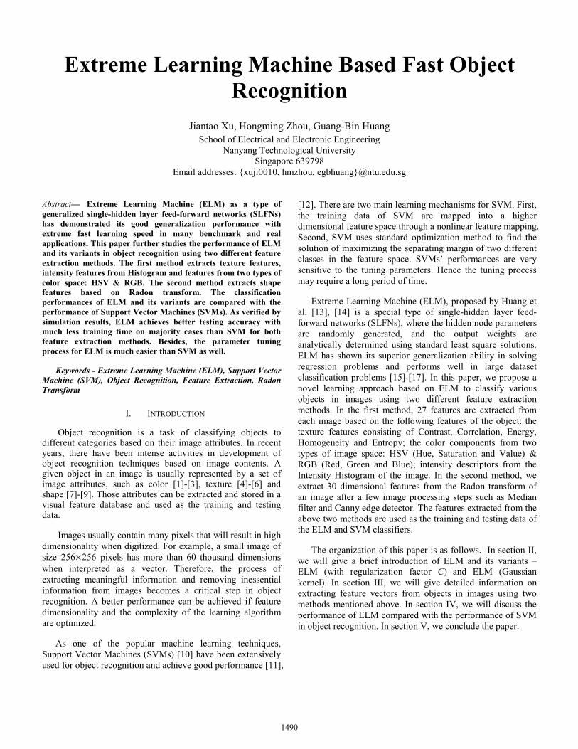
Fig. 3. Sample images from the second database

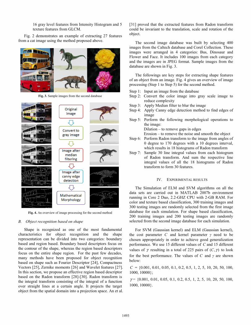
Fig. 4. An overview of image processing for the second method

B. Object recognition based on shape

Shape is recognized as one of the most fundamental characteristics for object recognition and the shape representation can be divided into two categories: boundary based and region based. Boundary based descriptors focus on the contour of the shape, whereas the region based descriptors focus on the entire shape region. For the past few decades, many methods have been proposed for object recognition based on shape such as Fourier Descriptor [24], Compactness Vectors [25], Zernike moments [26] and Wavelet features [27]. In this section, we propose an effective region based descriptor based on the Radon transform [28]-[30]. Radon transform is the integral transform consisting of the integral of a function over straight lines at a certain angle. It projects the target object from the spatial domain into a projection space. An et al.

[31] proved that the extracted features from Radon transform could be invariant to the translation, scale and rotation of the object.

The second image database was built by selecting 400 images from the Caltech database and Corel Collection. These images were arranged in 4 categories: Bus, Dinosaur and Flower and Face. It includes 100 images from each category and the images are in JPEG format. Sample images from the database are shown in Fig. 3.

The followings are key steps for extracting shape features of an object from an image. Fig. 4 gives an overview of image processing (Step 1 to Step 5) for the second method.

Step 1: Input an image from the database Step 2: Convert the color image into gray scale image to

reduce complexity Step 3: Apply Median filter to blur the image Step 4: Apply Canny edge detection method to find edges of

image Step 5: Perform the following morphological operations to

the image: Dilation – to remove gaps in edges Erosion – to remove the noise and smooth the object

Step 6: Perform Radon transform to the image from angles of 0 degree to 170 degrees with a 10 degrees interval, which results in 18 histograms of Radon transform

Step 7: Sample 30 line integral values from each histogram of Radon transform. And sum the respective line integral values of all the 18 histograms of Radon transform to form 30 features.

IV. EXPERIMENTAL RESULTS

The Simulation of ELM and SVM algorithms on all the data sets are carried out in MATLAB 2007b environment running in Core 2 Duo, 2.2-GHZ CPU with 2-GB RAM. For color and texture based classification, 300 training images and 300 testing images are randomly selected from the first image database for each simulation. For shape based classification, 200 training images and 200 testing images are randomly selected from the second image database for each simulation.

For SVM (Gaussian kernel) and ELM (Gaussian kernel), the cost parameter C and kernel parameter γ need to be chosen appropriately in order to achieve good generalization performance. We use 15 different values of C and 15 different values of γ resulting in a total of 225 pairs of ( , )C γ to look for the best performance. The values of C and γ are shown below:

C = {0.001, 0.01, 0.05, 0.1, 0.2, 0.5, 1, 2, 5, 10, 20, 50, 100, 1000, 10000};

γ = {0.001, 0.01, 0.05, 0.1, 0.2, 0.5, 1, 2, 5, 10, 20, 50, 100, 1000, 10000}.

1493

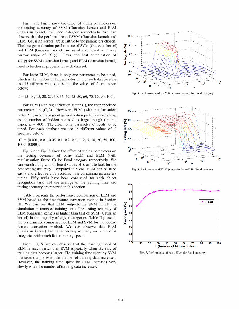
Fig. 5 and Fig. 6 show the effect of tuning parameters on the testing accuracy of SVM (Gaussian kernel) and ELM (Gaussian kernel) for Food category respectively. We can observe that the performances of SVM (Gaussian kernel) and ELM (Gaussian kernel) are sensitive to the parameters chosen. The best generalization performance of SVM (Gaussian kernel) and ELM (Gaussian kernel) are usually achieved in a very narrow range of ( , )C γ . Thus, the best combination of ( , )C γ for SVM (Gaussian kernel) and ELM (Gaussian kernel) need to be chosen properly for each data set.

For basic ELM, there is only one parameter to be tuned, which is the number of hidden nodes L . For each database we use 15 different values of L and the values of L are shown below:

L = {5, 10, 15, 20, 25, 30, 35, 40, 45, 50, 60, 70, 80, 90, 100}.

For ELM (with regularization factor C), the user specified parameters are ( , )C L . However, ELM (with regularization factor C) can achieve good generalization performance as long as the number of hidden nodes L is large enough (In this paper, L = 400). Therefore, only parameter C needs to be tuned. For each database we use 15 different values of C specified below:

C = {0.001, 0.01, 0.05, 0.1, 0.2, 0.5, 1, 2, 5, 10, 20, 50, 100, 1000, 10000}.

Fig. 7 and Fig. 8 show the effect of tuning parameters on the testing accuracy of basic ELM and ELM (with regularization factor C) for Food category respectively. We can search along with different values of L or C to look for the best testing accuracy. Compared to SVM, ELM can be used easily and effectively by avoiding time consuming parameters tuning. Fifty trails have been conducted for each object recognition task, and the average of the training time and testing accuracy are reported in this section.

Table I presents the performance comparison of ELM and SVM based on the first feature extraction method in Section III. We can see that ELM outperforms SVM in all the simulation in terms of training time. The testing accuracy of ELM (Gaussian kernel) is higher than that of SVM (Gaussian kernel) in the majority of object categories. Table II presents the performance comparison of ELM and SVM for the second feature extraction method. We can observe that ELM (Gaussian kernel) has better testing accuracy on 3 out of 4 categories with much faster training speed.

From Fig. 9, we can observe that the learning speed of ELM is much faster than SVM especially when the size of training data becomes larger. The training time spent by SVM increases sharply when the number of training data increases. However, the training time spent by ELM increases very slowly when the number of training data increases.

Fig. 5. Performance of SVM (Gaussian kernel) for Food category

Fig. 6. Performance of ELM (Gaussian kernel) for Food category

Fig. 7. Performance of basic ELM for Food category

1494

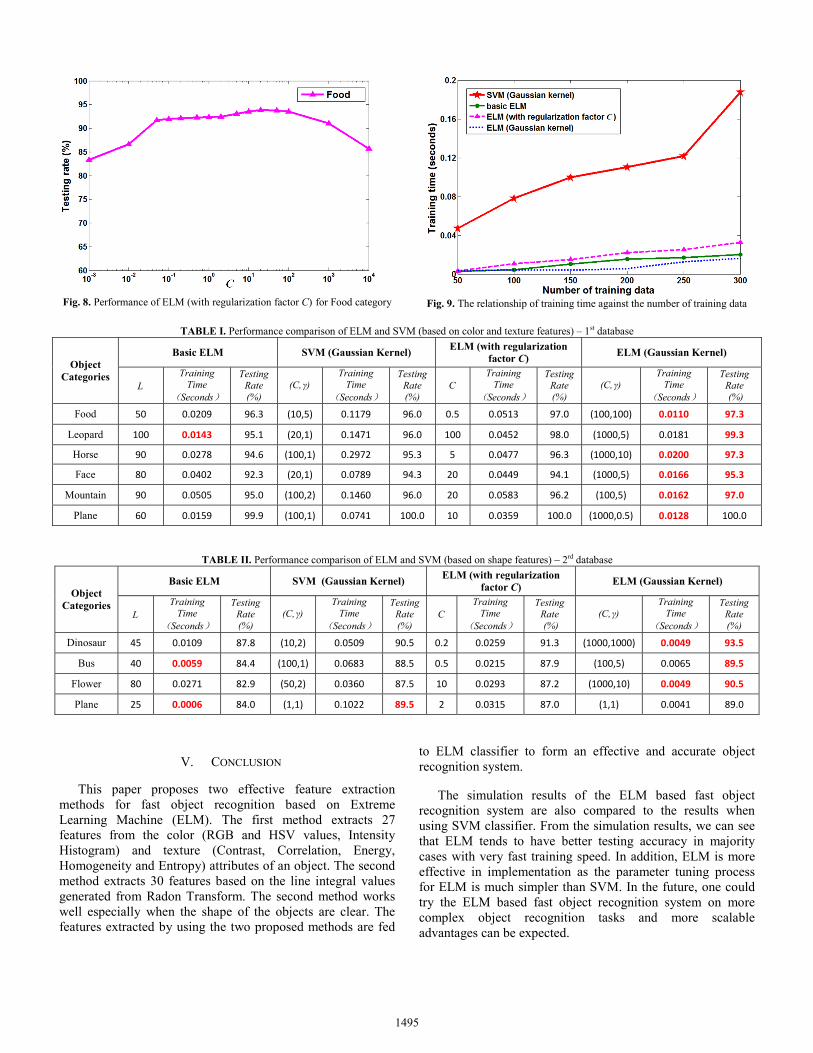
Fig. 8. Performance of ELM (with regularization factor C) for Food category

Fig. 9. The relationship of training time against the number of training data

TABLE I. Performance comparison of ELM and SVM (based on color and texture features) – 1st database

Object Categories

Basic ELM SVM (Gaussian Kernel) ELM (with regularization factor C) ELM (Gaussian Kernel)

L Training

Time（Seconds）

Testing Rate (%)

(C,γ) Training

Time（Seconds）

Testing Rate (%)

C Training

Time（Seconds）

Testing Rate (%)

(C,γ) Training

Time（Seconds）

Testing Rate (%)

Food 50 0.0209 96.3 (10,5) 0.1179 96.0 0.5 0.0513 97.0 (100,100) 0.0110 97.3

Leopard 100 0.0143 95.1 (20,1) 0.1471 96.0 100 0.0452 98.0 (1000,5) 0.0181 99.3

Horse 90 0.0278 94.6 (100,1) 0.2972 95.3 5 0.0477 96.3 (1000,10) 0.0200 97.3

Face 80 0.0402 92.3 (20,1) 0.0789 94.3 20 0.0449 94.1 (1000,5) 0.0166 95.3

Mountain 90 0.0505 95.0 (100,2) 0.1460 96.0 20 0.0583 96.2 (100,5) 0.0162 97.0

Plane 60 0.0159 99.9 (100,1) 0.0741 100.0 10 0.0359 100.0 (1000,0.5) 0.0128 100.0

TABLE II. Performance comparison of ELM and SVM (based on shape features) – 2rd database

Object Categories

Basic ELM SVM (Gaussian Kernel) ELM (with regularization factor C) ELM (Gaussian Kernel)

L Training

Time（Seconds）

Testing Rate (%)

(C,γ) Training

Time（Seconds）

Testing Rate (%)

C Training

Time（Seconds）

Testing Rate (%)

(C,γ) Training

Time（Seconds）

Testing Rate (%)

Dinosaur 45 0.0109 87.8 (10,2) 0.0509 90.5 0.2 0.0259 91.3 (1000,1000) 0.0049 93.5

Bus 40 0.0059 84.4 (100,1) 0.0683 88.5 0.5 0.0215 87.9 (100,5) 0.0065 89.5

Flower 80 0.0271 82.9 (50,2) 0.0360 87.5 10 0.0293 87.2 (1000,10) 0.0049 90.5

Plane 25 0.0006 84.0 (1,1) 0.1022 89.5 2 0.0315 87.0 (1,1) 0.0041 89.0

V. CONCLUSION

This paper proposes two effective feature extraction methods for fast object recognition based on Extreme Learning Machine (ELM). The first method extracts 27 features from the color (RGB and HSV values, Intensity Histogram) and texture (Contrast, Correlation, Energy, Homogeneity and Entropy) attributes of an object. The second method extracts 30 features based on the line integral values generated from Radon Transform. The second method works well especially when the shape of the objects are clear. The features extracted by using the two proposed methods are fed

to ELM classifier to form an effective and accurate object recognition system.

The simulation results of the ELM based fast object recognition system are also compared to the results when using SVM classifier. From the simulation results, we can see that ELM tends to have better testing accuracy in majority cases with very fast training speed. In addition, ELM is more effective in implementation as the parameter tuning process for ELM is much simpler than SVM. In the future, one could try the ELM based fast object recognition system on more complex object recognition tasks and more scalable advantages can be expected.

1495

ACKNOWLEDGMENT This research was sponsored by the grant from Academic

Research Fund (AcRF) Tier 1 of the Ministry of Education under project no. RG 22/08 (M52040128, Singapore).

REFERENCES [1] M. J. Swain and D. H. Ballard, “Color indexing,” International Journal

of Computer Vision, vol. 7, no. 1, pp. 11-32, 1991. [2] H. Nezamabadi and E. Kabir, “Image retrieval using histograms of

unicolor and bicolor blocks and directional changes in intensity gradient”, Pattern Recognition Letters, vol. 25, no. 14, pp. 1547- 1557, 2004.

[3] J. R. Smith and S.-F. Chang, “Single color extraction and image query,” In: Proceedings of International Conference on Image Processing, 1995, vol.3, pp.528-531.

[4] B. S. Manjunath and W. Y. Ma, “Texture feature for browsing and retrieval of image data,” IEEE Transactions on Pattern Analysis and Machine Intelligence , vol. 18, no. 8, pp. 837-842, 1996

[5] J. R. Smith and S. F. Chang, “Transform features for texture classification and discrimination in large image databases”, In: Proceedings of IEEE International. Conference on Image Processing, 1994.

[6] J. R. Smith and S. F. Chang, “Automated binary texture feature sets for image retrieval,” In: Proceedings of IEEE International Conference on Acoustics, Speech, and Signal Processing (ICASSP’96), 1996, vol. 4, pp. 2239-2242.

[7] L. D. Fu and Y. F. Zhang , “Medical Image Retrieval and Classification Based on Morphological Shape Feature,” In: Proceedings of 3rd International Conference on Intelligent Networks and Intelligent Systems (ICINIS), 2010, pp. 116-119.

[8] Z. Y. Wang, L. Bin, and Z. R. Chi , “Leaf Image Classification with Shape Context and SIFT Descriptors,” In: Proceedings of International Conference on Digital Image Computing Techniques and Applications (DICTA), 6-8 Dec 2011, pp. 650-654.

[9] Y. L. Xu, J. X. Qiu, and L. Ma, “Measurement and classification of shanghai female face shape based on 3D image feature,” In: Proceedings of 3rd International Congress on Image and Signal Processing (CISP), 16-18 Oct, 2010 , vol. 6, pp. 2588-2592.

[10] C. Cortes and V. Vapnik, “Support vector networks,” Machine Learning, vol. 20, no. 3, pp. 273–297, 1995.

[11] B. Y. Zhao and Y. J. Qi, “Image classification with ant colony based support vector machine,” In: Proceedings of 30th Chinese Control Conference, 22-24 July , 2011 , pp. 3260-3263.

[12] F. Jing, M. J. Li, and H. J. Zhang, “Entropy-based active learning with support vector machines for content-based image retrieval,” In: Proceedings of IEEE International Conference on Multimedia and Expo (ICME 2004), 27-30 June, 2004, vol. 1, pp. 85- 88.

[13] G.-B. Huang, Q. Y. Zhu, and C. K. Siew, “Extreme learning machine: a new learning scheme of feedforward neural networks,” In: Proceedings of 2004 International Joint Conference on Neural Networks (IJCNN 2004), 25-29 July, vol. 2, pp. 985-990.

[14] G.-B. Huang, Q. Y. Zhu, and C. K. Siew, “Extreme learning machine: theory and applications,” Neurocomputing, vol. 70, pp. 489-501, 2006.

[15] G.-B. Huang, X. Ding, and H. Zhou, “Optimization method based extreme learning machine for classification,” Neurocomputing, vol. 74, pp. 155-163, 2010.

[16] G.-B. Huang, H. Zhou, X. Ding, and R. Zhang, “Extreme Learning Machine for Regression and Multiclass Classification,” IEEE Transactions on Systems, Man, and Cybernetics - Part B: Cybernetics, vol. 42, no. 2, pp. 513-529, 2011.

[17] G.-B. Huang, D. H. Wang, and Y. Lan, “Extreme Learning Machines: A Survey,” International Journal of Machine Leaning and Cybernetics, vol. 2, no. 2, pp. 107-122, 2011.

[18] G.-B. Huang and L. Chen, “Convex incremental extreme learning machine,” Neurocomputing, vol. 70, no. 16–18, pp. 3056–3062, 2007.

[19] G.-B. Huang and L. Chen, “Enhanced random search based incremental extreme learning machine,” Neurocomputing, vol. 71, pp. 3460–3468, 2008.

[20] C. R. Rao and S. K. Mitra, Generalized Inverse of Matrices and Its Applications. New York: Wiley, 1971.

[21] R. Fletcher, Practical Methods of Optimization: Volume 2 Constrained Optimization. New York: Wiley, 1981.

[22] F-F. Li, R. Fergus, and P. Perona, “Learning generative visual models from few training examples: an incremental Bayesian approach tested on 101 object categories.” Workshop on Generative-Model Based Vision, 2004.

[23] Z. Wang, J. Li, and G. Wiederhold, “SIMPLIcity: Semantics-sensitive Integrated Matching for Picture Libraries,” IEEE Transactions on Pattern Analysis and Machine Intelligence, vol. 23, no. 9, pp. 947-963, 2001.

[24] D. Zhang and G. Lu, “Shape-based image retrieval using generic Fourier descriptor,” Signal Processing, vol. 17, pp. 825-848, 2002.

[25] C. Achard, J. Devars, and L. Lacassagne, “Object image retrieval with image compactness vectors,” In: Proceedings of 15th International Conference on Pattern Recognition, 2000, vol. 4, pp. 271-274.

[26] R. Mukundan and K. R. Ramakrishnan, “Fast computation of Legendre and Zernike moments,” Pattern Recognition, vol. 28, pp. 1433-1442, 1995.

[27] M. Jaisimha, “Wavelet features for similarity based retrieval of logo images”, In: Proceedings of SPIE Document Recognition III, San Jose, CA, 1996, vol. 2660, pp. 89–100.

[28] S. R. Deans, The Radon Transform and some of its Applications, New York: John Wiley & Sons, 1993.

[29] S. Tabbone, L. Wendling, and J.-P. Salmon, “A new shape descriptor defined on the Radon transform,” Computer Vision and Image Understanding, vol. 102, pp. 42-51, 2006.

[30] V. F. Leavers, “Use of the two-dimensional Radon transform to generate a taxonomy of shape for the characterization of abrasive powder particles,” IEEE Transactions on Pattern Analysis and Machine Intelligence, vol. 22, no. 12, pp. 1411-1423, 2000.

[31] Z. Y. An, Z. Y. Zeng and L. H. Zhou, “Content-Based Image Retrieval Based on the Wavelet Transform and Radon Transform,” In: Proceedings of 2nd IEEE Conference on Industrial Electronics and Applications (ICIEA 2007), 23-25 May 2007, pp. 1878-1881.

1496