Extraction Efficiency, Quality and Characterization of ...

Extraction Efficiency, Quality and Characterization of Typha latifolia L. Fibres for Textile

Applications

by

Koushik Chakma

A thesis submitted to the Faculty of Graduate Studies of

The University of Manitoba

in partial fulfilment of the requirements of the degree of

MASTER OF SCIENCE

Department of Biosystems Engineering

University of Manitoba

Winnipeg, Manitoba, Canada

Copyright © 2018 by Koushik Chakma

i

Abstract

The textile uses of the aquatic plant ‘Typha latifolia L.’ (genus Typha) have not been

previously explored. The current research is the first of its kind to examine the extraction, quality

and properties of this waste biomass fibre and compare them with the two most widely used fibres:

cotton and polyester, wool. It was found that Typha leaves and the core spongy tissue could be

transformed into fibres under controlled experimental conditions in aqueous alkaline solution

giving a yield range of 15% to 60%. The diameter of the Typha fibre is much higher than the

Cotton and wool while the moisture regain (%) and thermal resistance are comparable to these two

fibres.

SEM revealed a unique submicroscopic ‘crenelated’ structure and FTIR spectrum showed

the cellulose rich content in the Typha fibre. The cellulose content helped Typha fibre absorb the

reactive dyes and the dye exhaustion is similar or better than the cotton. However, the stiffness of

the Typha fibre is higher than the cotton and polyester, which would make Typha fibre difficult to

process in the Cotton spinning systems.

ii

Acknowledgements

Writing a scientific thesis is definitely a difficult task, and it was only possible because of

great support from some moral people. First of all, I want to express my sincere gratitude towards

my supervisor, Professor Dr. Mashiur Rahman, and my co-supervisor, Dr. Nazim Cicek. This

thesis would not have been completed successful without their intellectual guidance and valuable

advice. Most of all I am fully indebted to Dr. Rahman for his understanding, enthusiasm, wisdom,

patience and continuous supervision, which helped me to reach my dream. I am thankful to Dr.

Kevin McEleney from the Manitoba Institute for Materials (MIM), who gave me proper guidance

on how to use FTIR and KBr pellet preparation. My special appreciation goes to the Manitoba

Institute for Materials and Dr. Ravinder Sidhu, since she helped me to complete my research work

by providing opportunities to use the SEM machine and the Typha fibre morphological analysis

study. I am indebted to Mary Pelton, who supported me and provided me helpful guidance for

editing my thesis. Needless to say, another two important people, Nicholson and Joe Ackerman,

gave me tremendous support by providing Typha plant samples. I would like to thank the Natural

Sciences and Engineering Research Council of Canada (NSERC). It would have been impossible

without their assistance by helping me with their financial grant support.

Last but not least, my deepest appreciation to God, my parents, my wife, and my

classmates, esspecially Ikra Iftekhar Shuvo, Abdullah-Al-Mamun, Mahmudul Hasan, Yasin Sabik

and my roommates; they gave me great support. Undoubtedly, I would like to add them for being

a part of my success. They always supported me by helping me to survive all stresses and by not

letting me give up.

iii

Table of contents

Abstract……………………………………………………………………………………... i

Acknowledgements ………………………………………………………………………… ii

Table of contents………………………………………………………………………….... iii

Abbribation…………………………………………………………………………………. viii

List of Tables……………………………………………………………………………….. xi

List of Figures…………………………………………………………………………….... xiii

List of permitted copyrighted material from different sources……………………………... xxiv

1. Introduction………………………………………………………………………... 1

2. Literature review…………………………………………………………………... 9

2.1 History of textile fibres……………………………………………………………. 9

2.1.1 Natural cellulosic fibres……………………………………………………... 9

2.1.2 Common textile fibres ………………………………………………………. 15

2.2 Extraction of bast fibre……………………………………………………………. 18

2.2.1 Biological retting…………………………………………………………….. 19

2.2.2 Mechanical retting…………………………………………………………… 20

2.2.3 Chemical retting…………………………………………………………….... 20

2.2.4 Enzymatic retting…………………………………………………………….. 21

2.3 Characterization of bast fibre………………………………………………………. 22

2.3.1 Physical properties…………………………………………………………... 22

2.3.2 Spinning properties of fibres………………………………………………… 26

2.3.3 Blending properties………………………………………………………….. 28

2.3.4 Thermal properties…………………………………………………………... 28

2.4 Modification of bast fibre…………………………………………………………. 30

iv

2.4.1 Alkalization/mercerization…………………………………………………. 30

2.4.2 Dyeing of bast fibres………………………………………………………... 32

3. Materials and method…………………………………………………………….. 33

3.1 Retting and fibre extraction………………………………………………………. 34

3.2 Fibre extraction……………………………………………………………………. 35

3.3 Fibre characterization…………………………………………………………….. 37

3.3.1 Yield measurement…………………………………………………………. 38

3.3.2 Statistical analysis of Typha fibre length…………………………………… 39

3.3.3 Diameter measurement……………………………………………………... 39

3.3.4 Softness measurement…………………………………………………….... 40

3.3.5 Moisture regain (%) measurements……………………………………….... 40

3.3.6 Infrared (IR) spectrum study………………………………………………. 41

3.3.7 Thermal analysis…………………………………………………………… 41

3.3.8 Scanning electron microscopy (SEM)……………………………………… 42

3.3.9 Typha fibre dyeing with reactive dyes……………………………………… 43

3.3.10 Colour differences of dyed fibres………………………………………….. 44

3.3.11 Evaluation of dyeing performance (colorfastness to hot pressing) ………... 45

3.3.12 Statistical analysis……….............................................................................. 46

4. Extraction of Typha fibre…………………………………………………………. 47

4.1 General overview ………………………………………………………................ 47

4.1.1 Water retting………………………………………………………………. 47

4.1.2 Chemical retting……………………………………………………………. 50

4.2 Effect of various alkalis on fibre yield…………………………………………... 54

v

4.2.1 Fibre yield (%) from mixed plants…………………………………………. 54

4.2.2 Fibre yield (%) on hard stem (HS), soft stem (SS) and no stem (NS) plants.. 59

4.2.3 Data analysis………………………………………………………………… 60

4.3 Sources of flakes and barks in the fibre…………………………………………... 62

4.3.1 Extraction of fibre from various plant components………………………... 65

4.3.2 Summary………………………………………………………………….... 74

5. Textile characteristics of Typha fibre…………………………….......................... 75

5.1 Fibre morphology……………………………………………………………......... 75

5.1.1 Macrostructure of Typha fibre……………………………………………... 75

5.1.1.1. Fibre length…………………………………………………………... 75

5.1.1.1.1 Relationship between Typha plant length (cut length)

and fibre length ……………………………………………………….

77

5.1.1.2 Statistical results…………………...................................................... 77

5.1.1.3 Statistical analysis of Typha fibre length: Effect of treatment

on fibre length…………………………………………………………

80

5.1.1.4 Implications…………………………………………………………… 81

5.1.1.5 Fibre diameter………………………………………………………… 81

5.1.1.6 Statistical analysis…………………………………………………….. 84

5.1.1.7 Summary……………………………………………………………... 85

5.1.2 Microstructure of Typha fibre……………………………………………… 86

5.1.2.1 Cross-sectional features…………………………………………………

5.1.2.2 Longitudinal view of fibre………………………………………………

86

87

5.1.2.3 Submicroscopic structure………………………………………………. 88

vi

5.2. Typha fibre chemical composition by FTIR…………………………………. 91

5.3 Moisture regain of textile materials…………………………………………. 95

5.3.1 Summary…………………………………………………………………. 99

5.4 Thermal properties………………………………………………………….... 98

5.4.1 Burning behaviour of Typha fibre………………………………………… 99

5.4.2 Evaluation of Typha fibre thermal properties…………………………….. 101

5.4.3 Summary………………………………………………………………….. 104

5.5 Dyeing of Typha fibres with reactive dye………………………………………… 106

5.5.1 Evaluation of colour fastness of dyed Typha fibres……………..................... 110

5.5.1.1 Summary…………………………………………………………………. 118

5.5.2 Color differences of dyed Typha fibre…………………………..................... 119

5.6 Typha fibre hand properties………………………………………………………. 121

5.6.1 Summary………………………………………………………………………. 125

6. Conclusions and future work…………………………………………………….. 127

References………………………………………………………………………………….. 132

Appendix I…………………………………………………………………………………. 146

Appendix II………………………………………………………………………………… 152

Appendix III……………………………………………………………………………….. 155

Appendix IV……………………………………………………………………………….. 159

Appendix V………………………………………………………………………………… 160

Appendix VI………………………………………………………………………………. 163

Appendix VII………………………………………………………………………………. 164

Appendix VIII……………………………………………………………………………... 168

vii

Appendix IX………………………………………………………………………………. 170

Appendix X………………………………………………………………………………. 171

viii

Abbribation

American Association of Textile Chemists and Colorists (AATCC)

American Society for Testing and Materials (ASTM)

Analysis of Variance (ANOVA)

Ethylenediaminetetraacetic acid (EDTA)

Food and Agricultural Organization (FAO)

Food and Agricultural Organization Statistical Databases (FAOSTAT)

Fourier-transform infrared spectroscopy (FTIR)

Mixed Stem (MS)

Least Significant Difference (LSD)

Hard Stem (HS)

Scanning Electron Microscopy (SEM)

Soft Stem (SS)

No Stem (NS)

World Wide Fund (WWF)

Advanced Fibre Information System (AFIS)

Image analysis microscopy (IAM)

Polyethylene terephthalate (PET)

Polycyclic aromatic hydrocarbons (PAH)

Acrylic polyacrylontrile (PAN)

Polypropylene (PP)

Green House Gas (GHG)

High Volume Instrument (HVI)

International Organization for Standardization (ISO)

ix

List of Tables

Table 1.1: Country-based natural fibres production………………………………………..

6

Table 2.1: Chemical composition (%) of different plant fibres…………….……………...

11

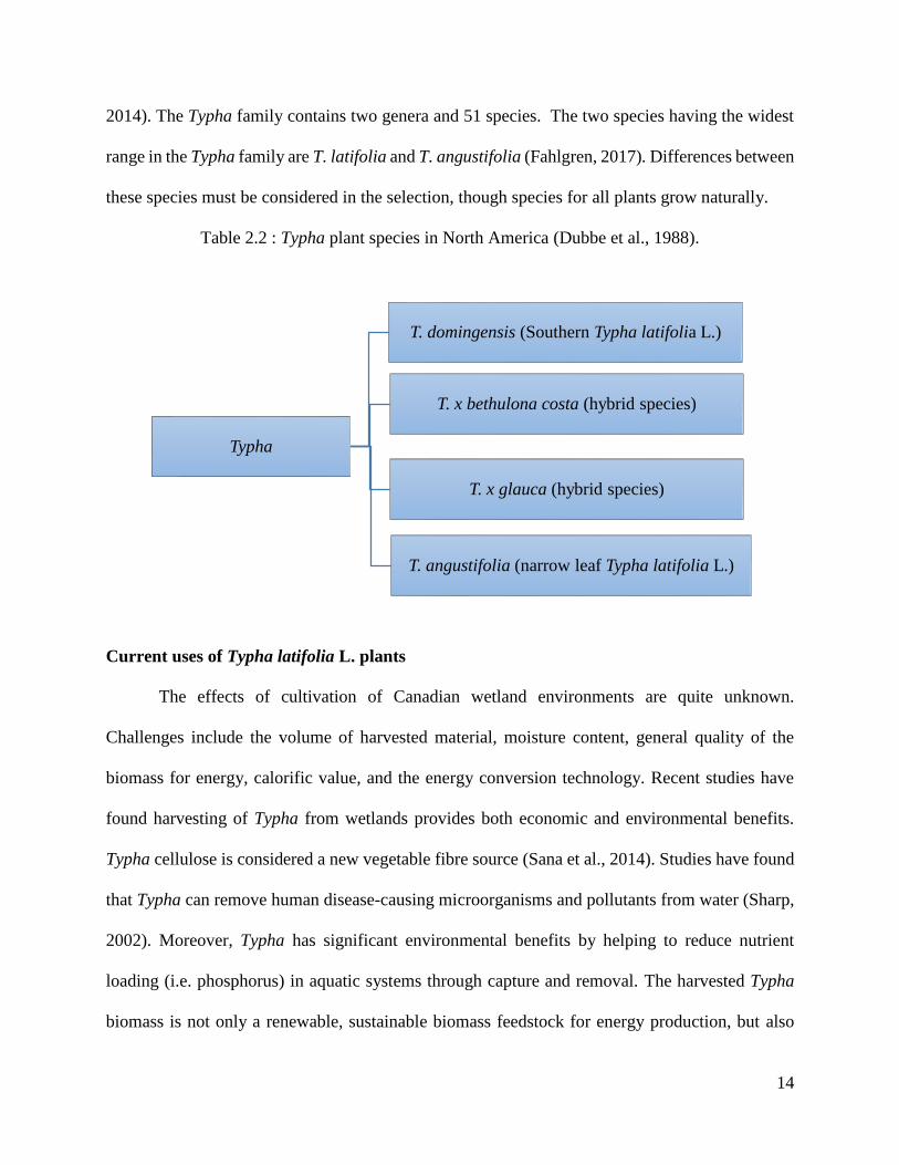
Table 2.2: Typha plant species in North America ………………………………………..

14

Table 2.3: Physical properties of polyester and Cotton fibres.……………………….

17

Table 2.4: Plant fibre degumming processes……………………………….......................

18

Table 2.5: Physical properties of major natural bast and leaf fibres ………………………

22

Table 2.6: Mechanical properties of major natural bast and leaf fibres …............................

23

Table 2.7: Ranking of fibre properties of Cotton for different short-staple

spinning systems and Length uniformity index……………………………………………

26

Table 2.8: Specific heat for textile fibres (Morton & Hearle, 2008)……………………....

29

Table 3.1: Chemicals and other materials used for Typha plant treatment………………... 34

Table 3.2: Typha plant fibre extraction methods ………………………………………….

35

Table 3.3: Experimental conditions for chemical treatment of Typha fibres (Based on

time variations) ……………………………………………………………………………

36

Table 3.4: Experimental conditions for alkali treatment of Typha fibres at high

temperature………………………………………………………………………………..

37

Table 3.5: LiOH treatment on Typha fibres (Based on time variations) …………………

37

Table 3.6: Characteristics of extracted Typha fibre……………………………………….

38

Table 4.1: Water retting of Typha plant………………………………………...................

49

Table 4.2: Fibre yield (%) for different chemical retting at room temperature (21°C) for

16 days……………………………………………………………………………………..

50

Table 4.3: Effect of different chemical treatments in fibre extraction…………………….

53

x

Table 4.4: Fibre yield (%) from ‘mixed plant’ in 3% KOH and 3% LiOH for different

treatment time……………………………………………………….....................………..

55

Table 4.5: Effect of time on the hard stems Typha fibre yield (%) in KOH (3%) Solution

at 80°C………………………………………………………………..................................

59

Table 4.6: Effect of time on the soft stems Typha fibre yield (%) in KOH (3%)

solution……………………………………………………………………………………..

60

Table 4.7: Fibre yield (%) for no stem plants in KOH (80°C & 95°C) and LiOH (80°C)

solution for different temperature………………………………………………………….

60

Table 4.8: Between-Subject Factors for fibre yield (%)…………………………………. 61

Table 4.9: Two-way ANOVA Results tests on the effect of temperature, time and alkali

type on fibre yield (%).…………………………………………………………………….

61

Table 4.10: Results of Post Hoc Tests for the effect of time on yield (%)………………... 62

Table 4.11: Plant morphology for hard, soft and no-stem plants with dimensions………… 65

Table 4.12: Fibre yield (%) and visual characteristics of fibres from different plant

segment, 3.0% KOH, 80°C after 8 hours……………………………………………………

73

Table 5.1: Statistical analysis on the relationship between plants cut length, and fibre

length for different treatments……………………………………………………………...

78

Table 5.2(a): Typha fibre diameter from various alkaline treatments.…………………….

81

Table 5.2(b): Fisher’s LSD test to compare the difference between pairs of means for

diameter of the thirteen Typha fibre………….....................................................................

82

Table 5.3(a): Diameter (µm) of Typha, Cotton, and Wool fibre……………………...........

83

Table 5.4(a): Statistical summary of Typha and Cotton fibre diameter…………………… 84

Table 5.4(b): Statistical summary of Typha and Wool fibre diameter……………………..

85

xi

Table 5.5: Summary of Typha microscopic study………………………………………… 91

Table 5.6: Peak assignments (cm-1) of IR spectra for Typha fibres………………………..

92

Table 5.7(a): Moisture regain (%) of Typha plants at various humidity and temperatures

………………………………...............................................................................................

95

Table 5.7(b): Moisture regain of Typha plant and fibre obtained from various treatments

and statistical analysis (ANOVA and Fisher’s LSD test)…………………………………..

97

Table 5.7(c): The comparison of moisture regain (%) between pair of means for Typha

plant and fibres by Fisher’s LSD test……………………………………………………...

98

Table 5.8: Burning Behaviour of Typha, Polyester and Cotton fibres……………………. 100

Table 5.9: Thermal properties of Typha plant, Typha fibre and Cotton fibre……………… 101

Table 5.10: Thermal properties of Typha and Cotton fibre with different temperatures

range……………………………………………………………………………………......

105

Table 5.11(a): Colour fastness rating in hot press method (damp pressing)

for Typha fibres……………………………………………………………….....................

113

Table 5.12(a): Colour fastness rating in hot press method (wet pressing) for Typha

fibres......................................................................................................................................

114

Table 5.11(b): Two-way ANOVA results tests on the effect of temperature and

treatments on colour fastness for damp pressing………………………………………….

115

Table 5.12(b): Two-way ANOVA results tests on the effect of temperature and

treatments on colour fastness for wet pressing……………………………………………

116

Table 5.13: Results of Post Hoc tukey tests for the effect of hot pressing to colour

fastness…………………………………………………………………………………...

117

Table 5.14: Typha fibre Color differences………………………………………………… 119

xii

Table 5.15: Dye Exhaustion by Typha Fibre………………………………………………. 120

Table 5.16(a): Typha fibre softness grading with other common fibres. ………………... 122

Table 5.16(b): Tukey post hoc multi-comparisons results for the effect of hand feel

properties on common fibres……………………………………………………………….

124

Table 6.1: Summary for fibre extraction, yield (%), textile properties of Typha fibre and

their suitability in textiles and apparel applications………………………………………..

127

xiii

List of Figure

Figure 1.1: Sources and classification of natural fibre……………………………………… 3

Figure 1.1: World production of natural fibres……………...……………………………… 7

Figure 2.1: Schematic diagram of basic structure of natural fibre cell structure of the plant…

10

Figure 2.2: Cross-section of Typha stem (1) and (2) aerenchyma tissue from Typha leaves…

12

Figure 2.3: World production of textile……………………………………………………… 17

Figure 2.4: Future forecast of global fibre demand out of 2013 as calculated by PCI……...

17

Figure 2.5: The length and diameter of major vegetable fibres……………………………… 24

Figure 2.6: Schematic presentation of alkali effect on swelling process in cellulose……….

30

Figure 2.7: (a) untreated molecular structure and (b) alkalization treatment cellulosic fibre

(Alkali treatment molecular structure depolymerizes and creates short length crystallites)…

31

Figure 3.1: Figure 3.1: Typha latifolia L. plants……………………………………………. 33

Figure 3.2: Dyeing process Curve………………………………………………………….. 44

Figure 3.3: CIELAB color space…………………………………………………………….

45

Figure 4.1: Original Typha plants………………………………………………………….. 49

Figure 4.2: Typha plant retted in water for 16 days at 21°C ………………………………………

49

Figure 4.3: Typha plant retted in water for 6 hours at 80°C………………………………………. 49

Figure 4.4: Typha plant retted in water for 90 days at 21°C.………………………………...

49

Figure 4.5: Appearance of Typha plant treated with acid (Sample: S1-CH3COOH) for 16

days at 21°C……………………………………………………………………………………………………………………………..

50

Figure 4.6: Appearance of Typha plant treated with alkali (Sample: S1-NaOH) for 16 days

at 21°C……………………………………………………………………………………….

50

xiv

Figure 4.7: Appearance of Typha plant treated with alcohol Sample: S1-CH3CH2OH) for

16 days at 21°C……………………………………………………………………………...

51

Figure 4.8: Appearance of Typha plant treated with enzyme (Sample: S1-Enzyme) for 16

days at 21°C…………………………………………………………………………………

51

Figure 4.9: Appearance of Typha plant treated with alkali (Sample: S3-NaOH) for

2h/1%/60°C………………………………………………………………………………….

53

Figure 4.10: Appearance of Typha plant treated with alkali (Sample: S4-CH3COOH) for

2h/1%/60°C………………………………………………………………………………….

53

Figure 4.11: Appearance of Typha plant treated with alkali (Sample: S5-NaOH) for

4h/3%/80°C………………………………………………………………………………….

53

Figure 4.12: Appearance of Typha plant treated with acid (Sample: S6- CH3COOH) for

4h/3%/80°C…………………………………………………………………………………………

53

Figure 4.13: Appearance of Typha plant treated with acid (Sample: S7- CH3COOH) for

8h/3%/80°C………………………………………………………………………………….

54

Figure 4.14: Appearance of Typha plant treated with Enzyme (Sample: S7-Enzyme) for

4h/3%/40°C………………………………………………………………………………….

54

Figure 4.15 (a): Appearance of Typha plant treated with alkali (Sample: S8-K1-MS) for 2h

at 80°C………………………………………………………………………………….........

56


at 80°C………………………………………………………………………………….........

56


at 80°C……………………………………………………………………………………….

56


xv

at 95°C………………………………………………………………………………………. 56


at 95°C ……………………………………………………………………………………

56


at 95°C…………………………………………………………………………………........

56


at 95°C……………………………………………………………………………………….

57

Figure 4.22 (a): Appearance of Typha plant treated with LiOH (Sample: S9-K8-MS) for 8h

at 80°C……………………………………………………………………………………….

57

Figure 4.23 (a): Appearance of Typha plant treated with LiOH (Sample: S10-L1-MS) for

2h at 80 °C…………………………………………………………………………………...

57


4h at 80°C…………………………………………………………………………………...

57


6h at 80°C……………………………………………………………………………………

57


8h at 80°C……………………………………………………………………………………

57

Figure 4.15 (a): Flake/bark material exists in (Sample: S8-K1-MS)……………………….. 58



Figure 4.24 (a): Flake/bark material exists in (Sample: S10-L2-MS)……………………….. 58

Figure 4.15 (b): Typha fibre treated with alkali (Sample ID: S8-K1-HS)

For 2h/3%/80°C…………………………………………………………………….... Appendix I

xvi

Figure 4.15 (c): Typha fibre treated with alkali (Sample ID: S8-K1-SS)

for 2h/3%/80°C…………………………………………………………………….... Appendix I

Figure 4.15 (d): Typha fibre treated with alkali (Sample ID: S8-K1-NS)

for 2h/3%/80°C…………………………………………………………………….... Appendix I


for 4h/3%/80°C…………………………………………………………………….... Appendix I


for 4h/3%/80°C…………………………………………………………………….... Appendix I


for 4h/3%/80°C…………………………………………………………………….... Appendix I


for 6h/3%/80°C…………………………………………………………………….... Appendix I


for 6h/3%/80°C…………………………………………………………………….... Appendix I


for 6h/3%/80°C …………………………………………………………………….... Appendix I


for 8h/3%/80°C…………………………………………………………………….... Appendix I


for 8h/3%/80°C…………………………………………………………………….... Appendix I


for 8h/3%/80°C…………………………………………………………………….... Appendix I


xvii

for 2h/3%/95°C…………………………………………………………………….... Appendix I


for 2h/3%/95°C…………………………………………………………………….... Appendix I


for 2h/3%/95 °C…………………………………………………………………….... Appendix I


for 4h/3%/95°C…………………………………………………………………….... Appendix I


for 4h/3%/95°C…………………………………………………………………….... Appendix I


for 4h/3%/95°C…………………………………………………………………….... Appendix I


for 6h/3%/95°C…………………………………………………………………….... Appendix I


for 6h/3%/95°C…………………………………………………………………….... Appendix I


for 6h/3%/95°C…………………………………………………………………….... Appendix I

Figure 4.22 (b): Typha fibre treated with KOH (Sample ID: S9-K8-HS)

for 8h/3%/80°C…………………………………………………………………….... Appendix I

Figure 4.22 (d): Typha fibre treated with with KOH (Sample ID: S9-K8-NS)

for 8h/3%/80°C…………………………………………………………………….... Appendix I

Figure 4.22 (c): Typha fibre treated with with KOH (Sample ID: S9-K8-SS)

for 8h/3%/80°C…………………………………………………………………….... Appendix I

xviii

Figure 4.23 (b): Typha fibre treated with LiOH (Sample ID: S10-L1-SS)

for 2h/3%/80°C…………………………………………………………………….... Appendix I

Figure 4.23 (c): Typha fibre treated with LiOH (Sample ID: S10-L1-HS)

for 2h/3%/80°C…………………………………………………………………….... Appendix I

Figure 4.23 (d): Typha fibre treated with LiOH (Sample ID: S10-L2-NS)

for 2h/3%/80°C …………………………………………………………………….... Appendix I

Figure 4.24 (b): Typha fibre treated with LiOH (Sample ID: S10-L2-HS)

for 4h/3%/80°C…………………………………………………………………….... Appendix I

Figure 4.24 (c): Typha fibre treated with LiOH (Sample ID: S10-L2-SS)

for 4h/3%/80°C…………………………………………………………………….... Appendix I


for 4h/3%/80°C…………………………………………………………………….... Appendix I


for 6h/3%/80°C…………………………………………………………………….... Appendix I


for 6h/3%/80°C…………………………………………………………………….... Appendix I


for 6h/3%/80°C…………………………………………………………………….... Appendix I


for 8h/3%/80°C…………………………………………………………………….... Appendix I


for 8h/3%/80°C…………………………………………………………………….... Appendix I


xix

for 8h/3%/80°C…………………………………………………………………….... Appendix I

Figure 4.27 (a): Bottom sponge diameter of Typha soft stems (HS) plant………………… 63

Figure 4.27 (b): Top sponge diameter of Typha soft stems (HS) plant………….................. 63

Figure 4.28 (a): Bottom sponge diameter of Typha soft stems (SS) plant……...................... 63

Figure 4.28 (b): Top sponge diameter of Typha hard stems (SS) plant………...................... 63

Figure 4.29: Different components of Typha plant leaves………………………………….. 64

Figure 4.30: Quadratic curve shape of plant………………………………………………... 64

Figure 4.36 (a): Cross-section whole (soft stem plant)……………………………………... 67

Figure 4.36 (b): Fibre (left) and bark/ Flakes, flakes (right) from Typha whole

(soft stem plant)……………………………………………………………………………..

67

Figure 4.31 (a): Cross-section of whole (hard stem plant) ………………………………… 67

Figure 4.31 (b): Fibre (left) and flakes/ bark (right) from Typha

whole (hard stem plant)……………………………………………………………………...

67

Figure 4.37 (a): Typha leaves (soft stem plant)……………………………………………… 68

Figure 4.37 (b): Fibre from Typha leaves (soft stem plant)………………………………… 68

Figure 4.32 (a): Typha leaves (hard stem plant)……………………………………………. 68

Figure 4.32 (b): Fibre from Typha leaves (hard stem plant)………………………………… 68

Figure 4.33 (a): Typha plant - hard wood bark with spongy tissue

(hard stem plant)……………………………………………………………………………..

68

Figure 4.33 (b): Fibre from Typha hard wood and with spongy tissue

(hard stem plant)……………………………………………………………………………..

68

Figure 4.33 (c): Hard stem + sponge [separated from sample 4.33 (b)]……………………. 68

Figure 4.38 (a): Typha plant - soft wood with spongy tissue (soft stem plant)………………. 69

xx

Figure 4.38 (b): Fibre from Typha soft wood and with spongy tissue

(soft stem plant)……………………………………………………………………………...

69

Figure 4.38 (c): Soft stem + sponge [separated from sample 4.38 (b)]…………………….. 69

Figure 4.34 (a): Typha plant hard wood bark (Hard stem)…………………………………. 69

Figure 4.34 (b): Typha fibre from hard woody bark treated with 3%KOH for 6h…………. 69

Figure 4.34 (c): Typha fibre from hard woody bark treated

with 3%KOH for 8h…………………………………………………………………………

70

Figure 4.34 (d): Typha fibre from hard woody bark treated

with 3%KOH for 12h………………………………………………………………………..

70

Figure 4.35 (a): Typha plant soft spongy tissue (hard stem plant)…………………………... 70

Figure 4.35 (b): Fibre from Typha soft spongy tissue (hard stem plant)……………………. 70

Figure 4.39 (a): Typha plant soft wood bark………………………………………………… 70

Figure 4.39 (b): Typha fibre from soft wood bark, 80°C/3%KOH/8h……………………… 70

Figure 4.39 (c): Typha fibre from soft wood bark, 80°C/3%KOH/12h…………. ………… 71

Figure 4.40 (a): Typha plant soft spongy tissue (soft stem plant)…………………………… 71

Figure 4.40 (b): Fibre from Typha soft spongy tissue (soft stem plant),

80°C/3%KOH/8h……………………………………………………………………………

71

Figure 4.41(a): Typha plant leaves (no stem plant)………………………………………… 71

Figure 4.41 (b): Fibre from Typha leaves with soft spongy tissue

(no stem plant), 80°C/3%KOH/8h…………………………………………………………..

71

Figure 5.1: A performance of fibre length in spinning processing ……………………….... 76

Figure 5.2 (a): Typha fibre length uniformity treated

with KOH (Sample S10-L4-MS)……………………………………………………………

79

xxi

Figure 5.2 (b): Typha fibre length uniformity treated

with KOH (Sample S8-K4-MS……………………………………………………………...

79

Figure 5.3: Fibre length variation between treated

Sample S8-K4-MS and S10-L4-MS………………………………………………………...

80

Figure 5.4: Diameter variation in 10 different places of Typha (a), Cotton (b),

Wool(c)……………………………………………………………………………………...

83

Figure 5.5: Cross-section of wool (a), Cross-section of Cotton (b), and Cross-section

of polyester (c) (Rao & Gupta, 1991; Rowland et al., 1976; and Brauer et al., 2008)……...

86

Figure 5.6: Cross-section of no stem plant (Left) and hard stem plant (Right)…………….. 87

Figure 5.7: Longitudinal view of Typha (a); Cotton (b); Wool (c); and Polyester (d)… 88

Figure 5.8: Cross-section of Typha plant with two distinct layers……………...................... 90

Figure 5.9: Individual Cell Size and distance of Typha fibre………………………………. 90

Figure 5.10: Single Typha fibre diameter…………………………………………………... 90

Figure 5.11: Polygonal ultimate cells with lumen size……………………………………... 90

Figure 5.12: ‘Crenelated’ (rectangular indentation) structure………………………………. 90

Figure 5.13: FTIR spectrum of extracted fibre from (a) Typha plant and

(b) S8-K2; (c) S5-NaOH; (d) S8-K3; (e) S10-L1; (f) S8-K4.….……………………. Appendix V

Figure 5.14(a): FTIR spectrum of Typha plant……………………………………….Appendix V

Figure 5.14(b): FTIR spectrum of S8-K2-MS Typha fibre………………………...…Appendix V

Figure 5.14 (c): FTIR spectrum of S5-NaOH-MS Typha fibre……………………....Appendix V

Figure 5.14(d): FTIR spectrum of S8-K3-MS Typha fibre………………………..….Appendix V

Figure 5.14(e): FTIR spectrum of S10-L1-MS Typha fibre……………………..….. Appendix V

Figure 5.15: Original fibres before burning test: polyester (a), Cotton (b), Typha (c) and

xxii

after burning test of polyester (d), Cotton (e) and Typha latifolia L.(f)………….................. 100

Figure 5.16(a): Virgin Typha plant…………………………………………………………. 102

Figure 5.16(b): Decomposed Typha plant……………………………………....................... 102

Figure 5.17(a): Virgin Typha fibre……………………………………………...................... 102

Figure 5.17(b): Decomposed Typha fibre…………………………………………………... 102

Figure 5.18(a): Virgin Cotton fibre ………………………………………………………… 102

Figure 5.18(b): Decomposed Cotton fibre…………………………………………….......... 102

Figure 5.19(a) to 5.22(a): Holding time (10 minutes) ………………………………Appendix VII

Figure 5.19(b) to 5.22(b): Holding time (20 minutes)……………………….……....Appendix VII

Figure 5.23(a) to 5.26(a): Holding time (10 minutes) ………………………………Appendix VII

Figure 5.23(b) to 5.26(b): Holding time (20 minutes) ………………………………Appendix VII

Figure 5.27(a) to 5.30(a): Holding time (10 minutes) ……………………………....Appendix VII

Figure 5.27(b) to 5.30(b): Holding time (20 minutes) ……………………….……..Appendix VII

Figure 5.31 (a) to 5.32(a): Holding time (20 minutes) ……………………….…….Appendix VII

Figure 5.31(b) to 5.32(b): Holding time (20 minutes) …………………………..….Appendix VII

Figure 5.33: Changes in L* Value with temperature for Cotton and Typha fibres………… 106

Figure 5.34: Dyed blue Typha fibre (Sample ID: S5-NaOH-MS/4h/80C)………………... 107

Figure 5.35: Dyed blue Typha fibre (Sample ID: S8-K2-MS/4h/ 80C)…………………… 107

Figure 5.36: Dyed blue Typha fibre (Sample ID: S10-L2-MS/4h/80C)…………………... 108

Figure 5.37: Dyed Cotton fibre……………………………………………………………... 108

Figure 5.38: Dyed blue Typha fibre (Sample ID: S8-K3-MS/ 6h/80C)…………………… 108

Figure 5.39: Dyed blue Typha fibre (Sample ID: S10-L1-MS/2h/80C)…………………... 108

Figure 5.40: Dyed blue Typha fibre (Sample ID: S9-K5-MS/2h/95C)……………………. 108

xxiii

Figure 5.41: Temperature at 50°C dyed samples…………………………………………… 109



Figure 5.44: Temperature at 80°C dyed sample …………………………………………… 109

Figure 5.45: Different temperatures demonstrated in hot plate…………………………….. 110

Figure 5.46: Shade variation in hot plate (left: over 60 C)

(middle: less than 50 C) and (right: 50 C)………………………………………………..

110

Figure 5.47: Dye liquor evaluation by Hunter lab for sample S10-L2-MS

for sample S10-L2-MS………………………………………………………………………

120

xxiv

List of copyrighted material for which permission was obtained

Figure 1.1: World production of natural fibres (million tonnes, average). Used with permission

from John Wiley and Sons.

Figure 2.1: Schematic diagram of basic structure of natural fibre cell structure of the plant Used

with permission from Author Rudi Dungani.

Figure 2.2: Cross-section of Typha stem from Typha plants. Used with permission from Author

Richard Sojda & Kent L. Solberg.

Figure 2.5: The length and diameter of major vegetable fibres. Used with permission from John

Wiley and Sons.

Figure 2.7: Schematic presentation of alkali effect on swelling process in cellulose. Used with

permission from John Wiley and Sons.

1

CHAPTER 1: INTRODUCTION

Over the past few decades, the global production and consumption of textiles has increased

due to population growth and improvements in living standards (Wang, 2006). The growth rate of

textile industries has helped to develop strong economies; however, these industries face major

challenges, especially regarding environmental pollution. At the present time, high demand and

low cost, coupled with higher dimensional stability of fibres and the wide range of applications,

have created a great expansion of synthetic fibres (Collier et al., 2009; Khan, 2016).

Most synthetic fibres are costly, not easily biodegradable and responsible for

environmental pollution (Salit, 2014). The primary resource material for polyester (polyethylene

terephthalate or PET) is petroleum, which is acknowledged to be hazardous to the environment

(Zupin & Dimitrovski, as cited in Dubrovski, 2010). Polyester and other synthetic polymer fibres

(acrylic, polyamide, and polypropylene) are non-renewable and require large quantities of

petrochemicals and energy that contribute to environmental pollution (Zupin & Dimitrovski, as

cited in Dubrovski, 2010). During polyester (PET) production, polycyclic aromatic hydrocarbons

(PAH) are emitted into the air, producing high amounts of toxicity: a concern for human safety

(Shen et al., 2010).

More sustainability in textile industries and more sustainable products to meet basic human

needs require the development of both ecological integrity and social equity (Sun, as cited by Wool

& Sun, 2005). Research is focusing on natural fibres as they have dynamic properties that could

be replaceable instead of synthetic fibres. Natural fibre has been used since 7000 BC for different

purposes such as paper, rope, and clothing (Kozlowski, 2012a). Presently, many potential plant

fibres such as coir (Cocos nucifera L. adapted from Hoffmann, 1884), sisal (Agave sisalana P.

adapted from Mussig, 2001), jute (Corchorus olitorius L., adapted from Curtis, 1828), flax (Linus

2

usatissimum L., adapted from Meyers, 1906), banana (Musa textile adapted from Meyers, 1906),

pineapple, hemp (Cannabis sativa L. adapted from Pabst, 1887), canola (Brassica napus L.,

adapted from Khan, 2016), ramie (Boehmeria nivea H.; adapted from Mussig, 2001), and Kenaf

(Hibiscus cannabinus L. adapted from www.wikipedia.org/wiki/Kenaf), are used as a resource for

industrial materials in composites and reinforced polymer applications (Salit, 2014).

Natural fibre properties depend mainly on the nature of the plant, locality in which it is

grown, age of the plant, and the extraction method used. Natural fibres are a widely abundant

renewable resource. The traditional natural fibres collected from various sources and their

classification are given in Figure 1.1. Nature offers a large number of fibrous cellulosic materials

from which fibre may be extracted. Various parts of the plant such as the woody core, bast, leaf,

cane, straw, grass, and seed are valuable not only for textiles but also for building materials, human

and animal food, agro-fine chemicals, biomass energy and environmentally friendly cosmetics

(Kozlowski, 2012a). The part of the plant being used determines the fibre length: stems and leaves

yield longer fibres than fruits or seeds (Blackburn, 2005).

Fibres have been defined by the Textile Institute as units of matter having a length at least

100 times their diameter or width (Fedorak P. M., as cited in Blackburn, 2005). The characteristic

dimensions of fibres are the basis of their use: individual fibres (or elements of a continuous

filament) weigh only a few micrograms, and their length/width ratio is at least 1000:1 (Moncrieff,

1963). The traditional natural fibre sources include cotton, wool, and silk. Bast or leaf fibres –

Flax, Kenaf, Hemp and, Raime have been developed to transform a variety of textile materials of

all natural fibres. Cotton has botanical name known as Gossypium herbaceum, adapted from

Meyers, 1906.; it is the most commonly used fibre and has the most globally significant demand,

accounting for 35.7 % of the textile market worldwide (Kozlowski, et al., 2012a).

3

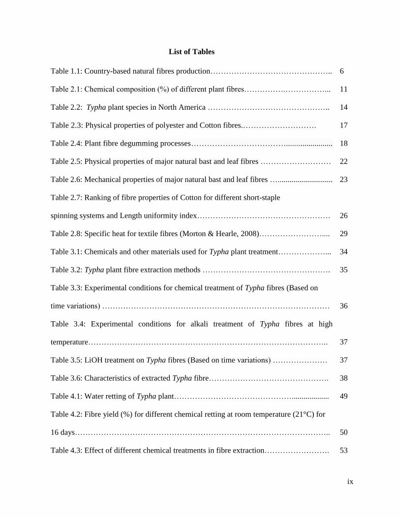
Figure 1.1: Sources and classification of natural fibre (Kozlowski, 2012a).

More than 80 countries produce Cotton, and it represents 2.5% of the entire cultivated crop

land of the world (Rashid et al., 2016). Production of Cotton fibre has a significant impact on the

environment, as Cotton is considered the most pesticide intensive crop in the world (Rashid et al.,

2016). To produce one kilogram of Cotton requires enormous amounts of pesticide and 10,000

litres of water. In other words, it takes 2700 litres of water to make one Cotton t-shirt (WWF,

n.d.,). The production of Cotton is responsible for the rapid consumption of natural resources and

damage to the fertility of the soil (Judkins, 2008; Khan, 2016). Additionally, agricultural land is

often used for Cotton production, thereby having a major impact on food supplies (Judl et al.,

2016).

Natural Fibers

Mineral Animal Bacterial Vegetable

Root

Rhectophyllum

camerunense

Wood

Hardwood

Softwood

Husk

Barley

Maize

Wheat

Fruit

Coir

Seed

Gossypium

Kapok

Milkweed

Grass

Maize

Oat

Rice

Rye

Wheat

Bast

Flax

Cannabis

Jute

Kenal

Mesta

Boehmeria

Roselle

Urena

Stalk

Esparto

Miscanthus

Reed

Cane

Bagasse

Bamboo

Leaf and leaf sheath

Abaca

Banana

Cabuja

Curaua

Date palm

Henequen

Ixtle

Pineapple

Sisal

Cellulose and lignocellulosic

4

Due to the problems of Cotton and Cotton production, researchers have focused on other

natural fibres, called bast fibres, such as linum, corchorus, cannabis, and boehmeria. These are

environmentally friendly, and their usability is increasing day by day. Bast fibres have more cost-

efficient production and broad product possibilities. All bast fibres have renewable properties with

high biomass production per unit land area (Kozlowski, 2012a). Moreover, leaf and crop waste

left in the field transforms into organic materials, thereby reducing demand for supplementary

chemical fertilizers for subsequent crops (Kozlowski, 2012a). Bast fibre, being of agro-origin, has

some unique characteristics such as high strength, good frictional property, tenacity, very high

modulus, low breaking elongation, high moisture and good dyeability, using different dyes

(reactive direct, vat), good heat and sound insulation properties and low production cost

(Kozlowski, 2012a).

Despite their advantages, the share of bast fibres in global clothing industries is very low

because of some major limitations such as: insufficient spinning properties (breaking twist angle,

single fibre entity, poor bending properties for preparation of yarns), lack of suitable large-scale

fibre extraction equipment, and costly methods of degumming (Mather & Wardman, 2015;

Kozlowski, 2012a). The fibre yield (%) from bast fibre is also very low (10 to 15%). For example,

brassica fibre yield is only 13.82 % and virgin brassica fibre is very stiff, and like all other bast

fibres, its usage is very limited in apparel applications (Khan, 2016).

The global market share of bast fibre extracted from the stems of the cannabis plant is only

0.09 %, which is negligible (Figure 1.2). The stiff surface of the cannabis fibre makes it difficult

to process on a Cotton spinning system (Ali, 2013). Sometimes the fibre has an irregular surface

due to the incomplete removal of the non-cellulosic materials (lignin, pectin). Cannabis production

requires higher investments for specialized machinery in order to produce quality spun yarns.

5

Linum, also a bast fibre, is rigid and difficult to process in Cotton spinning systems and it is costlier

on specialized machinery (Minotte & Franck, 2005). According to Kozlowski et al. (2012a), the

higher cost of spinning fine yarn comes from the low speed of spinning and the low automation

of the process. Recent studies found that brassica fibres solve the environmental problem as fibres

are obtained from waste biomass; however, the yield of brassica fibres is low, as mentioned earlier,

which is similar to other bast fibres. Further, virgin brassica fibres are stiff and cannot be processed

in Cotton spinning machinery without further machine and fibre modifications. For these reasons,

bast fibre is not being widely used for fabric.

Considering the above factors, an effort has been made to develop a new textile material

with new characteristics, one that is environmentally sustainable, comfortable and industrially

suitable. Therefore, researching and developing the extraction and establishment of new cellulose-

based textile material is vital.

6

Table 1.1: Country-based natural fibres production (Source: FAO, 2014).

Fibre production from natural sources

Countries Banana Coconut Pineapple Sugar

cane

Rice Oil palm

Corchorus Kenaf Linum Agave Abaca Kapok

Brazil 6.90 2.82 2.48 0.74 11.76 1.34 26.71 14.20 0.71 0.25 1.20 na

China 10.55 0.25 1.00 125.54 203.29 0.70 0.17 0.08 0.47 0.15 0.65 0.06

India 24.87 11.93 1.46 341.20 159.20 na 1.98 0.12 0.22 0.21 na na

Indonesia 6.19 18.30 1.78 33.70 71.28 120.00 0.007 4.35 na 0.03 0.05 0.03

Malaysia 0.34 0.61 0.33 0.83 2.63 100.00 0.002 0.01 na na na 0.008

Philippine 9.23 15.35 2.40 31.87 18.44 0.48 0.002 na 0.002 na 0.08 na

Thailand 1.65 1.01 2.65 100.10 38.79 12.81 0.06 1.30 0.01 0.003 na 0.07

USA 0.01 na 0.20 27.91 8.63 na na na 0.004 na na na

Vietnam 1.56 1.31 0.540 20.08 44.04 na 0.02 8.20 na 0.01 0.01 0.003

*na: Not applicable.

7

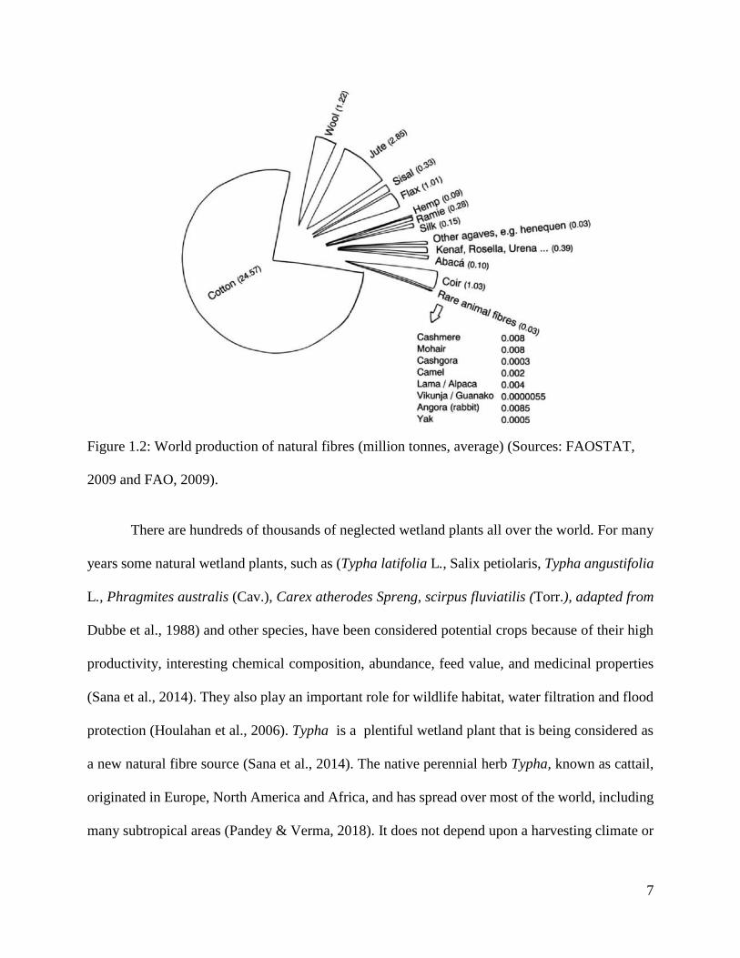
Figure 1.2: World production of natural fibres (million tonnes, average) (Sources: FAOSTAT,

2009 and FAO, 2009).

There are hundreds of thousands of neglected wetland plants all over the world. For many

years some natural wetland plants, such as (Typha latifolia L., Salix petiolaris, Typha angustifolia

L., Phragmites australis (Cav.), Carex atherodes Spreng, scirpus fluviatilis (Torr.), adapted from

Dubbe et al., 1988) and other species, have been considered potential crops because of their high

productivity, interesting chemical composition, abundance, feed value, and medicinal properties

(Sana et al., 2014). They also play an important role for wildlife habitat, water filtration and flood

protection (Houlahan et al., 2006). Typha is a plentiful wetland plant that is being considered as

a new natural fibre source (Sana et al., 2014). The native perennial herb Typha, known as cattail,

originated in Europe, North America and Africa, and has spread over most of the world, including

many subtropical areas (Pandey & Verma, 2018). It does not depend upon a harvesting climate or

8

perfect growing conditions, as do other bast fibres. Typha can have significant environmental

benefits. The plants are ecofriendly and used to clean soil polluted by heavy metals [cadmium

(Cd), lead (Pb), copper (Cu), and zinc (Zn)] (Kozlowski, 2012b). Typha grows rapidly, is widely

distributed and available locally, is renewable, mouldable, hydroscopic, recyclable, versatile, non-

abrasive, porous, viscoelastic, easily available in many forms, biodegradable, and reactive

(Maizatul et al., 2012). These features could make the Typha fibre appropriate as a raw material

for industrial use. For apparel and industrial applications, it is important to understand the physical

and chemical properties of Typha plants and fibre.

Typha fibre has some unique characteristics; it is environmentally friendly and has

multifunctional properties such as thermal insulation (Luamkanchanaphan et al., 2012), reinforced

composite, (Wuzellaa et al., 2011), nutrient seizing and watershed management (Grosshans, 2014),

and handmade papermaking (Bidin et al., 2015). For these reasons, it is worth exploring if Typha

can be used in the apparel and textile industry. To start, an effective way to extract the fibre from

the plant is needed. A specific method for extracting fibre from Typha does not exist yet; traditional

methods need to be explored and analyzed for feasibility in textile applications.

It is hypothesized that the Typha fibre can be useful for textile uses. Therefore, to determine

if this is possible, the following criteria need to be met:

1. Identify a standard extraction method of Typha fibre from Typha plants;

2. Optimize the extraction parameters for maximum yield and fibre quality (time,

temperature and concentration);

3. Determine major textile properties of Typha fibre such as: physical properties,

chemical properties, and thermal properties.

9

CHAPTER 2: LITERATURE REVIEW

2.1 History of textile fibres

Any product made from fibrous materials is considered a textile. Cellulose fibres found in

nature have been used for cloth for 4000 to 5000 years (Kozlowski, 2012a; Kozlowski &

Mackiewicz -Talarczyk, 2012). Weaving and knitting are the two most common methods used for

manufacturing textiles.

Cotton was produced in Egypt around 12000 BC, and in India approximately 1500 BC;

Linum fibre use goes back to 6500 BC (Kozlowski & Mackiewicz-Talarczyk, 2012). Silk, a protein

filament fibre, is produced from silkworms that Chinese people have bred as early as 3000 BC.

The history of Cotton documents its use for mankind since 5000 BC in India and the Middle East

(Kozlowski, 2012a).

2.1.1 Natural cellulosic fibres

Vegetable or cellulosic fibres can be obtained from different parts of the plant such as seed

(Cotton, kapok, coir), bast (linum, corchorus, cannabis, boehmeria, kenaf), and leaf (agave,

abaca), and they are classified according to their source in the plant (Nayak et al., as cited by

Kozlowski, 2012b, p. 314 –315). Marques et al. (2010) state that cell characteristics of size,

thickness, and the shape and thickness of the lumen are used to identify a vegetable fibre. Natural

fibres found in the stem and leaf parts of the plant consist of a complex composite of cellulose,

hemicelluloses, lignins and aromatics, waxes and other lipids, ash and water-soluble compounds

that are glued together in different layers of the cell walls (Akin, 2010). Cellulose itself is a linear

polymer composed of β -d -glucose units, linked together by β -1,4-glycosidic bonds to expand a

linear polymer chain (Kozlowski, 2012a). Hemicellulose exists in the natural fibres which are more

coherent between cellulose and lignin (Thomas et al., as cited by Kalia et al., 2011). The degree of

10

polymerization of cellulose varies according to the plant species (7000 dp–15000 dp) (Akin, 2010).

Usually the sclerenchyma elongated cells give supporting tissue in plants, providing much

strength, and rigidity (Kozlowski, 2012a). Two important properties, xylem and phloem tissue of

monocotyledonous and dicotyledonous, are involved fibres of plant stems and leaves (Smole et

al., 2013).

Plant cells have distinctive cell walls: the primary wall cover with a loose irregular linkage

of closely packed cellulose microfibrils, and the secondary cell wall that is divided into three sub-

layers (Kozlowski, 2012a). The primary and secondary cell wall together can be considered a

composite matrix of lignin and hemicellulosic polysaccharides (Krässig, 1993). The middle layer

has helically arranged microfibrils that give the fibre its mechanical properties. Specific fibres

have different microfibrillar orientation in three sub-layers (Krässig, 1993; Smole et al., 2013).

When the secondary cell wall is thicker, the lumen becomes smaller. Cellulose forms a crystalline

structure with regions of high order orientation amorphous regions of low order orientation.

Figure 2.1: Schematic diagram of basic structure of natural fibre cell structure of the plant

(Dungani et al, 2016). (Image removed due to copy right restrictions.)

The chemical composition as well as the morphological microstructure of vegetable

fibres is extremely complex due to the hierarchical organization of the different compounds

11

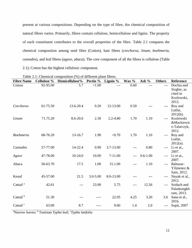
present at various compositions. Depending on the type of fibre, the chemical composition of

natural fibres varies. Primarily, fibres contain cellulose, hemicellulose and lignin. The property

of each constituent contributes to the overall properties of the fibre. Table 2.1 compares the

chemical composition among seed fibre (Cotton), bast fibres (corchorus, linum, boehmeria,

cannabis), and leaf fibres (agave, abaca). The core component of all the fibres is cellulose (Table

2.1); Cotton has the highest cellulosic component.

Table 2.1: Chemical composition (%) of different plant fibres.

Fibre Name Cellulose % Hemicellulose% Pectin % Lignin % Wax % Ash % Others Reference

Cotton 92-95.00 5.7 <1.00 --- 0.60 --- --- Dochia and

Sirghie, as

cited in

Kozlowski,

2012.

Corchorus 61-75.50 13.6-20.4 0.20 12-13.00 0.50 --- --- Roy and

Lutfar,

2012(b).

Linum 71.75.20 8.6-20.6 2.30 2.2-4.80 1.70 1.10 --- Kozlowski

&Mackiewic

z-Talarczyk,

2012.

Boehmeria 68-76.20 13-16.7 1.90 <0.70 1.70 1.10 --- Roy and

Lutfar,

2012(a).

Cannabis 57-77.00 14-22.4 0.90 3.7-13.00 --- 0.80 --- Li et at.,

2007.

Agave 47-78.00 10-24.0 10.00 7-11.00 --- 0.6-1.00 --- Li et at.,

2007.

Abaca 56-63.70 17.5 1.00 15.1.00 --- 1.10 --- Baltazar-

YJimenez &

Sain, 2012.

Kenaf 45-57.00 21.5 3.0-5.00 8.0-13.00 --- --- --- Nayak et al.,

2012.

Cattail a

42.61 --- 23.90 5.75 --- 12.56 --- Sridach and

Paladsongkh

ram, 2013.

Cattail b 51.30 --- ---- 22.05 4.25 3.20 3.6 Sana et al.,

2016.

Cattail c 63.00 8.7 ---- 9.60 1.4 2.0 --- Sopit, 2007

aNarrow leaves; b Tunisian Typha leaf; cTypha latifolia

12

Introduction of bast fibres

Bast fibres have been used for over 8000 years

(Smole et al., 2013). They are collected from stems or

stalks of dicotolydenous plants. Their woody core

structure is surrounded by a stem that consists of a

number of fibre bundles or aggregates (Hearle, 1963)

having 10 to 25 elementary fibres 2 to 5 mm long and

10 - 50 μm in diameter (Thomas et al., as cited by Kalia

et al., 2011). Elementary fibrils and bundles are

cemented by lignin and pectin intercellular substances,

which must be extracted to obtain the fibres (Mohanty,

2005).

Bast fibres usually contain higher amounts of cellulose (57%–77%), while hemicellulose

(9%–14%) and lignin (5%–9%) content is lower compared to woody core fibres (Stevulova, 2014).

Currently, bast fibres are raw materials not only for the textile industry, but also for modern

environmentally-friendly composites in different applications such as building materials, particle

boards, insulation boards, food, cosmetics, and medicine, and are a source for other biopolymers.

Several species of Typha exist in North America and other parts of the world. The differences

between them must be considered in the selection of a species for a particular site (Dubbe et al.,

1988). Typha latifolia L. (broadleaf cattail), Typha angustifolia L. (narrow leaf cattail), and Typha

x glauca (a hybrid of the other two species), known as wetland plants and charecteristics are

aboveground leaves, below ground rhizome system, and recognizable inflorescence (Dubbe et al.,

1988).

Figure 2.2: Cross-section of Typha stem

from Typha plants (Sojda and Solberg,

1993).

13

Species selection may affect yield potential, tolerance to various site conditions, nutrient

uptake patterns, evapotranspiration rates, characteristics as fibre, and energy (Dubbe et al., 1988).

The stem height of Typha ranges from 1 to 3 m with collective 12-16 linear and flat leaves that are

15 to 25 mm wide (Grace & Harrison, 1986). The Typha stalk is structured in one-piece, consisting

of several reciprocally incorporated sheets. Each of these sheets is divided by thin walls into

several individual areas. Every area of the sheet is divided into very fine 10 μm to 50 μm open

pores. Both individual Typha sheets and the stalks consist of enough strong outer walls to fully

retain their processing, i.e. cutting, sorting, knotting into bales, and pressing to a given density.

The inner layer of Typha in the individual areas is filled with very weak and brittle material

(Vėjelienė et al., 2011). The special characteristics of Typha include good tensile strength of stem

fibre and elastic sponge-like tissue, and leaves that are tear and break resistant. These

characteristics provide remarkable load-bearing capacity and excellent insulation property (Krus

et al., 2014). In the most common form of vegetable fibres, the cellulose structure depends mainly

on pectin and hemi-cellulose. In the randomly oriented amorphous regions, the higher the

amorphousness, the greater is the vapour water or dye absorption rate of the fibre. In the crystalline

regions, where the polymers are oriented or aligned longitudinally or parallel along the fibre axis,

hydrogen bonding occurs (Thomas et al., as cited by Kalia et al., 2011).

Classification of the Typha plant

Typha has mostly colonial, rhizomatous, perennial characteristics in the division of

Magnoliophyta, class Liliopsida, subclass Commelinidae, order Typhales, family Typhaceae (Sana

et al., 2014). A monocotyledonous plant, Typha are considered important wetland plants of

shoreline areas in temperate and boreal North America (Smith, 1986) and are also distributed

throughout the tropical and temperate regions of the world in marshes and wetlands (Sana et al.,

14

2014). The Typha family contains two genera and 51 species. The two species having the widest

range in the Typha family are T. latifolia and T. angustifolia (Fahlgren, 2017). Differences between

these species must be considered in the selection, though species for all plants grow naturally.

Table 2.2 : Typha plant species in North America (Dubbe et al., 1988).

Current uses of Typha latifolia L. plants

The effects of cultivation of Canadian wetland environments are quite unknown.

Challenges include the volume of harvested material, moisture content, general quality of the

biomass for energy, calorific value, and the energy conversion technology. Recent studies have

found harvesting of Typha from wetlands provides both economic and environmental benefits.

Typha cellulose is considered a new vegetable fibre source (Sana et al., 2014). Studies have found

that Typha can remove human disease-causing microorganisms and pollutants from water (Sharp,

2002). Moreover, Typha has significant environmental benefits by helping to reduce nutrient

loading (i.e. phosphorus) in aquatic systems through capture and removal. The harvested Typha

biomass is not only a renewable, sustainable biomass feedstock for energy production, but also

Typha

T. domingensis (Southern Typha latifolia L.)

T. x bethulona costa (hybrid species)

T. x glauca (hybrid species)

T. angustifolia (narrow leaf Typha latifolia L.)

15

mitigates greenhouse gas (GHG) emissions. The recovery of phosphorus could be a precious

resource for global food security (Grosshans, 2014).

In addition, researchers have established that Typha can be harvested and used as a source

of “biofuel,” meaning the plant material can be dried and burned for energy, reducing consumption

of fossil fuel such as coal. Typha leaves may even be fermented to produce ethanol which has

excellent energy properties for displacing gasoline (Lakshman, 1984 as cited by Grosshans, 2014).

The phosphorus from Typha ash could be used as a crop fertilizer. Typha leaves have an

interesting soft open-cell spongy tissue that provides an excellent insulating effect, fire protection,

noise protection, elasticity or hydrophobicity (Krus et al., 2014). Typha stock comprises resilient,

natural monocultures with an annual production rate of 15 to 20 tonnes of dry matter per hectare

(Krus et al., 2014). This enormous growth rate of Typha may be appropriate as a raw material for

industrial use. The Typha is a natural neglected plant (NNP) whose chemical constitutions are

shown in Table 2.1.

2.1.2 Common textile fibres

Cotton is known as a plant seed fibre of the genus Cotton and the purest form of cellulose

available in nature (Nevell, as cited by Shore, 1995). Cotton is very prominent in the textile

industry because it has many desirable fibre properties making it a major fibre for textile

applications. The properties of strength and good absorbency make it a comfortable and durable

apparel fabric.

The commercial development of man-made fibres began in the early 20th century. The

study of polymer thread-like molecules found great progress in the 1920s and 1930s, and in the

1930s Wallace H. Carothers developed the first known polymer fibre, Nylon (Khan, 2016), which

was developed and manufactured by DuPont in the United States starting in March 1953 (Collier

16

et al., 2009). The commercial development of man-made fibres experienced much growth during

the 1940s and expanded rapidly after World War II. Synthetic/man-made fibres have been in major

use for general textiles since the 1950s. Today, many other classes of polymer have been developed

for different purposes and applications such as polyester, polyamides, olefins, polyethylene

terephthalate (PET), acrylic polyacrylontrile (PAN) and polypropylene (PP) (Cook, 2001).

Polyester fibres can be defined as fibre-forming substances of an aliphatic hydro-carbon

(—CO·O·CH2·CH2·O·CO—) of linear condensation polymers composed of at least 85% by

weight of an ester of a substituted aromatic carboxylic acid produced by melt-spinning and

drawing (Cook, 2001). In aliphatic sequence, monomers are flexible at room temperature and

bonded with weak van der Waals force. Polyester fibre is known for its many uses, and when

blended with other fibres, it helps to increase durability of the product. Since Cotton and polyester

are similar moduli they are ideal for blending.

Currently, textile fibres are not limited to traditional cloth manufacturing, but have diverse

applications in almost all sectors such as agriculture, aquaculture, horticulture and forestry;

reinforced polymer composites are used in aircraft, marine craft, automobiles, civil infrastructure,

medical prosthesis and all kind of sports and leisure materials (Salit, 2014; Mohammed et al., 2015;

Mussig, 2010).

Global fibre consumption increases as new products are developed. The world fibre

consumption is 90% for yarn, 7% for nonwoven, and the rest for filling, cigarette filters and so on

(Lawrence, 2003). The latest figures, published in 2001, showed 53% of the world production of

textiles is synthetic polyester fibre; whereas, Cotton was only 33.3%. The other natural and

synthetic fibre production is: wool 2.3%; cellulosics 4%; corchorus 5.8%; linen 0.3%; boehmeria

1.1%; and silk 0.1%, respectively.

17

Figure 2.3: World production of Textile (Lawrence, 2003; pp.24).

Table 2.3 Physical properties of polyester and Cotton fibres (Ali, 2013; Kozlowski, 2012a).

Fibre

Name

Length (mm)

textile fibre

from stem

Finished

Fibre

Length for

spinning

(mm)

Finished

Fibre

Diameter

(microns,

µg/inch)

Density

(g/cm³)

Moisture

(%) (65%

RH,

21°C)

Fibre

fineness

(μm)

Tenacity

(g/den)

Cotton 15-56 15 - 56 2-6.5 1.52 -1.56 8-11.0 16.0-21.0 1.7-6.3

Polyester Controllable Controllable Controllable 1.36 -1.41 0.4 1.3-22.0 3.0-7.0

Figure 2.4: Future forecast of global fibre demand out of 2013 as calculated by PCI fibres. (Source:

www.textileworld.com).

Synthetic

53.01%

Cellulosics

4.00%Cotton (Gossypium)

33.31%

Wool

2.30%

Corchorus

5.80%

Linen

1.10%Boehmeria nivea

0.34%Silk

0.14%

World Production of Textile

Synthetic Cellulosics Gossypium Wool Corchorus Linen Boehmeria nivea Silk

18

Figure 2.4 shows the demand for three dominant fibres, Cotton, polyester and cellulose,

across history. Throughout the years, the demand for Cotton and polyester fibre has remained fairly

constant, with cellulosic fibre experiencing a slight growth of 5 million tons. The consulting firm,

England-based PCI Fibres, calculates that the estimated polyester fibre demand will increase until

2030.

2.2 Extraction of bast fibre

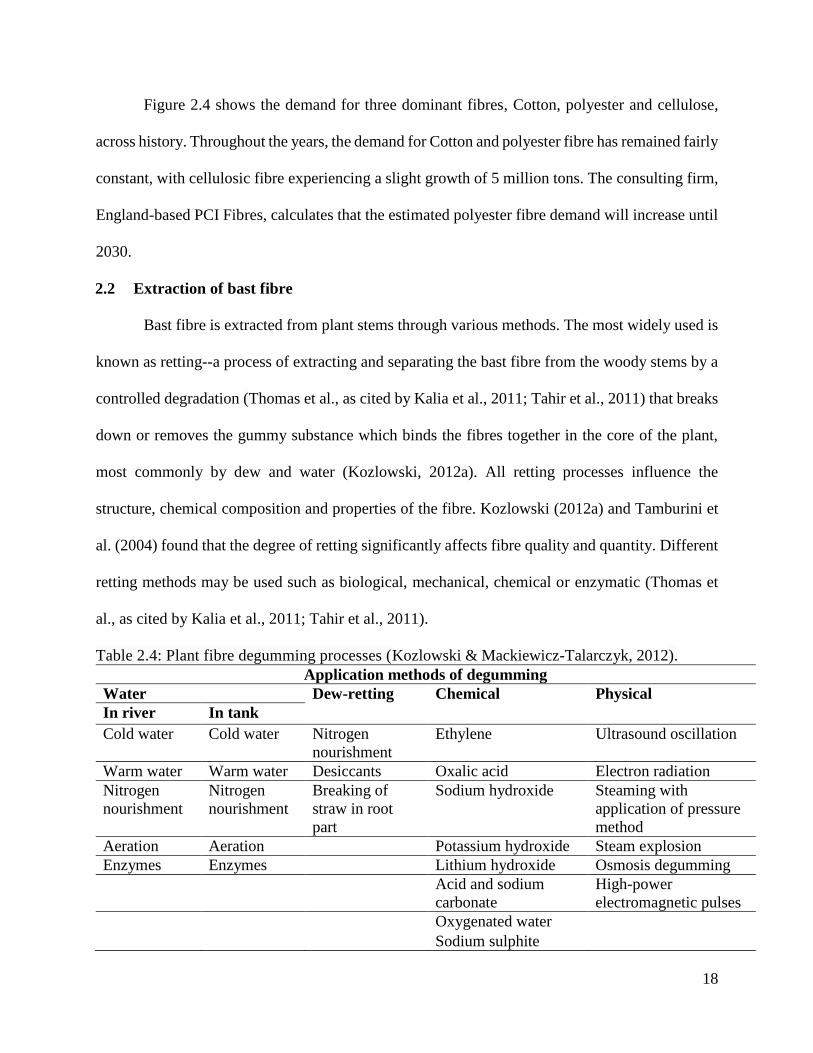
Bast fibre is extracted from plant stems through various methods. The most widely used is

known as retting--a process of extracting and separating the bast fibre from the woody stems by a

controlled degradation (Thomas et al., as cited by Kalia et al., 2011; Tahir et al., 2011) that breaks

down or removes the gummy substance which binds the fibres together in the core of the plant,

most commonly by dew and water (Kozlowski, 2012a). All retting processes influence the

structure, chemical composition and properties of the fibre. Kozlowski (2012a) and Tamburini et

al. (2004) found that the degree of retting significantly affects fibre quality and quantity. Different

retting methods may be used such as biological, mechanical, chemical or enzymatic (Thomas et

al., as cited by Kalia et al., 2011; Tahir et al., 2011).

Table 2.4: Plant fibre degumming processes (Kozlowski & Mackiewicz-Talarczyk, 2012).

Application methods of degumming

Water Dew-retting Chemical Physical

In river In tank

Cold water Cold water Nitrogen

nourishment

Ethylene Ultrasound oscillation

Warm water Warm water Desiccants Oxalic acid Electron radiation

Nitrogen

nourishment

Nitrogen

nourishment

Breaking of

straw in root

part

Sodium hydroxide

Steaming with

application of pressure

method

Aeration Aeration Potassium hydroxide Steam explosion

Enzymes Enzymes Lithium hydroxide Osmosis degumming

Acid and sodium

carbonate

High-power

electromagnetic pulses

Oxygenated water

Sodium sulphite

19

2.2.1 Biological retting

Biological retting is divided into two processes, natural and artificial (Thomas et al., as

cited by Kalia et al., 2011). Biological retting involves in-field or dew retting, and cold water

retting. Dew or field retting is the most commonly applied process to achieve satisfactory retting

as a result of weather conditions, appropriate moisture and temperature ranges (Kozlowski &

Mackiewicz-Talarczyk, 2012; Thomas et al., as cited by Kalia et al., 2011; Tahir et al., 2011).

Stems from cut crops are spread over the surface of the field for 2-8 weeks depending on the

location, and the degree of retting required (Kozlowski, 2012a). The stems are exposed to light,

weather and temperature conditions. During the in-field retting process, microorganisms attack

the stems and break down the cementations that bind together the fibre bundles (Kozlowski &

Mackiewicz-Talarczyk, 2012). When sufficiently retted, the colour of the stems turns dark grey.

Under-retting creates difficulty in separating and further processing the fibre; over retting degrades

fibre quality; therefore, the process must be stopped at an appropriate time (Thomas et al., as cited

by Kalia et al., 2011). Field retting can minimize labour input because it does not require the

transport of crops as the retting methods are applied in the field, maximizing agricultural efficiency

and cost (Kozlowski & Mackiewicz-Talarczyk, 2012).

The process of submerging plant stems into different water sources, such as a huge water

tanks, ponds, rivers or vats, uses anaerobic bacteria to breakdown the pectin of the plant straw

bundles (Thomas et al., as cited by Kalia et al., 2011). This retting process depends on water type,

the temperature of the retting water and any bacterial inoculum. Water retting is often considered

the best separation method compared to other methods as it takes only 7 to 14 days (Kozlowski &

Mackiewicz-Talarczyk, 2012, Akin, D.E. as cited as Mussig, 2010). Applying heat between 30C

to 40C may reduce the process time and provides a high quality fibre (Thomas et al., as cited by

20

Kalia et al., 2011); however, it leads to environmental pollution due to unacceptable organic

fermentation in waste waters (Thomas et al., as cited by Kalia et al., 2011).

Another type of biological retting is artificial retting, which produces homogeneous fibres,

works with warm water, and takes 3 to 5 days for high quality, clean fibres (Thomas et al., as cited

by Kalia et al., 2011). The plant bundles are soaked in warm water tanks, and the best fibres are

separated from the woody parts at completion of the retting process.

2.2.2 Mechanical retting

During mechanical retting, mechanical actions (scotching, hacking, hammer mill, roller

mill) separate the fibre from the woody core part of the plant. Mechanical retting is a more

economical and easy procedure using either field dried or slightly retting plant straw (Thomas et

al., as cited by Kalia et al., 2011); however, it produces poorer fibres which are much coarser

compared to dew or water retting fibres (Thomas et al., as cited by Kalia et al., 2011).

2.2.3 Chemical retting

In chemical retting, the plant stems are immersed into heated tanks containing solutions of

sulphuric acid, chlorinated lime, sodium or potassium hydroxide and soda ash (Thomas et al., as

cited by Kalia et al., 2011). The extraction process of removing non-cellulosic materials uses hot

alkaline solution (Williams et al., 2011). This is commonly a dispersion and emulsion-forming

process that uses surface active agents to remove unwanted non-cellulosic constituents which bind

the fibres. It is the shortest process, taking only few hours, compared to days required for other

retting methods. The yield of fibres in the chemical retting process is very good, but it adds an

additional cost for the final products (Kozlowski & Mackiewicz-Talarczyk, 2012). From

environmental aspect, cotton does not require any retting and hemp and flax needs bio-retting

(Thomas et al., as cited by Kalia et al., 2011), whereas, chemical retting process has huge impects

21

on environmental pollution (Muthu, 2018). Therefore, it is urge to think the chemical retting

westage water could be reusable by biological enzymetic treatment (Muthu, 2018), waste water

tearment plant (Kumar and Saravanan, as cited by Muthu, 2018) will less impact on

environment.

2.2.4 Enzymatic retting

A common process called microbial/enzymatic retting extracts good quality cellulosic

fibres from vegetable plants such as cannabis, linum and corchorus (Thomas et al., as cited by

Kalia et al., 2011; Tahir et al., 2011). Enzymes produced by fungus or bacteria weaken or remove

the pectinic glue that bonds the fibre bundles and release the cellulosic fibres. This process is costly

because it needs huge quantities of enzymes and equipment (Kozlowski & Mackiewicz-Talarczyk,

2012).

2.3 Characterization of bast fibre

2.3.1 Physical properties of textile fibres

The properties of natural fibres refer to fibre diameter, structure, degree of polymerization,

crystal structure and source. A plant fibre shows various properties due to different growth

conditions (Eder & Burgert, as cited by Mussig, 2010). To be suitable for apparel applications, a

fibre must demonstrate essential fundamental properties of strength, tenacity and spinning power

depending on the end uses. Fibres need strength when twisted together. This property implies a

measure of cohesion between the individual fibres which will give strength to the yarn. Spinning

of a fibre means there is a certain amount of surface roughness or serration promoted by fineness

and uniformity of diameter. An important property of a fibre is flexural rigidity that increases with

the decrease in fibre linear density. Fine fibres have lower bending rigidity (Kaushik, Tyagi, &

Chatterjee, 1990). Some researchers have studied fibre properties, which are influenced by fibre

22

type, spinning system and twist on yarn flexural rigidity. Other fundamental properties which are

desirable for a fibre are durability, softness, absence of undesirable colour and affinity for dyes.

A potential textile fibre must have some potential textile properties. The ability to

withstand tensile force (tenacity) and extension at break are considered important parameters for

the manufacturing of yarn in different processing stages such as spinning, winding, warping, sizing

and fabric formation (weaving and knitting). In addition, fibre properties and behaviour directly

affect fabric performance. The essential parameters for a textile fibre include length, flexibility,

cohesiveness, and sufficient strength. Other significant properties include elasticity, fineness,

uniformity, durability, and luster. For example of physical and mechanical properties are shown

in Table 2.5 and 2.6 which are collected from literature (Franck, 2005).

Table 2.5: Physical properties of major natural bast and leaf fibres (Franck, 2005).

Physical

characteristics

Fibre Types

Linum Cannabis Kenaf Corchorus Boehmeria Nettle Agave

Length of fibre

(mm)

300-600 1000-3000 900-1800 150-360 1500 19-80 600-1000

Ultimate

length (mm)

13-60 5-55 1.5-11 0.8-6 40-250 5.5 0.8-8

Diameter (µm) 12-30 16-50 14-33 5-25 16-125 20-80 100-400

Weight per

length

1.7-17.8 3.20 50 13.27 4.6-6.4 -- 9-400

Density

(g/cm3)

1.4 1.4 -- 1.4 1.4 -- 1.2-1.45

23

Table 2.6: Mechanical properties of major natural bast and leaf fibres (Franck, 2005).

Physical

characteristics

Fibre Types

Linum Cannabis Kenaf Corchorus Boehmeria Agave

Tensile strength

(GPa)

0.90 0.31-0.39 0.18 0.22-0.53 0.29 0.08 - 0.839

Specific tensile

strength (GPa m3/kg)

0.60 0.07- 0.42

Flexibility modulus

(GPa)

85 2.5-13 3-98

Specific flexibility

modulus (GPa m3

/kg)

71 9.0 3.82

Tensile modulus

(GPa)

13 15

Elongation at break

(%)

1.8-3.3 1.7-2.7 1.7-2.7 1.0-2.0 2.3-4.6 2.9 - 6.8

Specific tenacity

(GPa m3/kg)

0.37 0.44

Elasticity modulus

(GPa)

0.26 - 0.32 0.15 - 0.19

Fibre length

Length is an important attribute of a textile fibre that influences process efficiency, quality

of yarn (Kumar, 2015), performance and price (Morton & Hearle, 2008). Short or staple fibres are

measured in inches or fraction of an inch: for example, 3/4 inch to 18 inches. All natural fibres

except silk are staple fibres. Since staple fibres are a finite length, they are much more uniform in

length than filament fibres. Filament fibres are long, often an indefinite length, measured in yards

or meters. Silk filament is 360-1200 meters; man-made filament length can be continuous.

Fibre length can be determined from a fibrograph (Kumar, 2015) in which a formation

beard of parallel fibres passes through an optical sensing point. This beard is formed when fibres

from a sample are automatically grasped by a clamp, then combed and brushed into parallel

orientation (Cotton Incorporated, 2016). Fibre diameter, fineness and maturity are three important

physical properties that impact the spinning process and end uses of a fibre (Montalvo, 2005).

24

Fibre maturity in Cotton refers to the degree of cell wall development (Khan, 2016).

Fibre diameter

The fibre diameter, usually expressed in micrometer (µm), defines the distance across its

cross section, or the length of a straight line through the center of a circle or sphere. In natural

fibres, the diameter varies from one part of the fibre to another because of irregularities in fibre

size. In contrast, manufactured fibres usually have a uniform diameter throughout, for example the

diameter of polyester fibres used for apparel is presumed to be circular (Stout, 1960). Fibre

diameter has significant importance in intermediate (sliver, yarn) and final products (fabric and

apparel). Fibre diameter (d) affects numerous physical characteristics of yarn such as: yarn

thickness or linear density in Ne (English Cotton count systems) (∝1/d), yarn bending rigidity (∝

d) and extension (∝ d), yarn twist (∝ 1/d) and some important fabric characteristics such as fabric

Figure 2.5: The length and diameter of major vegetable fibres. The linear curve represents an aspect

ratio of 100 and estimate mean vaule with dotline shows the range of literature data (Ageeva et al.

(2005), Aldaba (1927), Angelini et al.(2000), Ashori et al. (2006), Baley (2002), Jarman and laws

(1965), Khalil et al.(2008), Kozlowski et al.(2005), Kundu (1956), Leupin (2001), McDougall et

al. (1993), Morvan et al.(2003), Mukherjee and Satyanarayana(1986) and Ruys et al.(2002), as

cited in Mussig, 2010).

25

weight, drape, handle, and comfort. Moreover, the price of a textile end product often depends on

fibre diameter, as finer materials cost more.

Fibre fineness defines the diameter, cross-sectional area and linear density (weight per unit

length) (Kumar, 2015). The mature Cotton fibre cell wall shows 50% to 80% moisture in the cell

wall; whereas, immature fibre shows 30% to 45%, and dead fibres less than 25% (Kumar, 2015).

A large number of finer fibres results in a stronger yarn. However, an abundance of dead fibre

results in difficulties in the spinning process and a low strength yarn. These two attributes of

maturity and fineness are measured using several methods including the USTER, Advanced Fibre

Information System (AFIS), Shirley Development Fineness Maturity Tester, polarized light

microscopy, fibre cross-section image analysis microscopy (IAM), and near infrared spectroscopy

(Kim et al., 2014). The micronaire value of Cotton depends on specific surface and is influenced

by both fibre fineness and maturity. A low micronaire value indicates finer fibres; whereas, high

micronaire values usually indicate coarser fibres, which is problematic in Cotton spinning systems

and yarn evenness (Montalvo, 2005).

Textile fibres must demonstrate special characteristics such as minimum length, tensile

strength, higher initial modulus and cohesiveness with pliability. Tenacity, as defined by Kumar

(2015), is the breaking force of a material divided by the linear density of the unstrained material

and can be expressed as tex, lbf / tex, kgf / tex, cN / tex.

Tenacity = Breaking force/ tex. (tex is a unit of measurement of liner mass density of fibre)

The tensile strength of corchorus and kenaf provides much stronger tenacity than other

fibres because of their small elongation at break with higher initial modulus (Krishnan et al., as

cited in Franck, 2005). Different plants have different cellulosic morphological alignments

producing variations in mechanical properties.

26

The bonding natures between fibres, the orientation of the fibres within the bundles and

micro fibril angle of cell walls (Eder & Burgert, as cited by Mussig, 2010) help to connect

neighbouring fibres. Two adjacent fibres have opposite cellulose fibril orientations in the

connected cell walls. Because fibres are bonded with tight interlocking, fibre bundles are stiffer

than single fibres (Eder & Burgert, as cited by Mussig, 2010). Usually, the Pressley Index (PI) is

used to indicate the fibre bundle strength. A fibre bundle with a PI value of 75-80 would be

considered medium strength.

2.3.2 Spinning properties of fibres

Conditions of fibre length, fineness, strength, stiffness and single fibre entity determine the

spinability of a fibre and the success of the subsequent weaving process. Spinning properties

determine the quality of a fibre and increase the values in the textile market. The summary in Table

2.7 provides a ranking of the importance of fibre properties using three Cotton spinning methods:

ring, rotor and air jet spinning (Gordon, as cited by Gordon & Hsieh, 2007) which can be used for

characterization of the spinning properties of fibres.

Table 2.7: Ranking of fibre properties of Cotton for different short-staple spinning systems and

length uniformity index (Gordon, as cited by Gordon & Hsieh, 2007; Kumar, 2015).

Priority ranking of

property

Ring spinning Rotor spinning Air-jet spinning

1 Flexibility Flexibility Flexibility

2 Single fibre entity Single fibre entity Single fibre entity

3 Length Strength Length

4 Strength Fineness Trash

5 Fineness Length Fineness

6 N/A Trash Strength

HVI length uniformity Index

Degree of uniformity Very high High Intermediate Low Very Low

Range in (%) >85 83-85 80-82 77-79 <77

27

Fibre fineness, a factor which limits the spinability of a yarn, is a measure of thickness in

the crosswise direction (Kumar, 2015). In a given cross section of yarn, different numbers of fibres

can be accommodated depending on fineness of the fibres. When more fibres are in a given cross

section they are fine; fewer fibres are coarser. Fineness also controls spinning limit, luster and

drape of the textile materials. For Cotton yarn, a micronnaire value of 3 - 4.9 is considered to be

medium range fineness (Ali, 2013). Fibre length is another parameter for uniformity and tenacity

of fibre spinning. Length uniformity is the ratio of the mean length and upper half mean length of

the fibrograph, expressed as a percentage. Kumar (2015) defined fibre length measured by

selecting average length of the longer one-half of the fibres, usually from the upper half mean

length value obtained from a high-volume instrument (HVI) or 2.5% span length gained from a

fibrogram. For example, if the fibres in a bale were all of equal length, then the mean length and

upper half mean length would be equal and would give a uniformity index of 100.

Shorter fibres are problematic during the spinning process and produce lower quality yarn.

Fibre length impacts spinning limit, yarn strength, yarn evenness, handle and luster of the product,

yarn hairiness and productivity.

Fibre cohesive properties contribute to yarn strength. In Cotton, the natural breaking

strength of individual Cotton fibres helps in spinning. The yarn strength correlates highly with

fibre strength. The minimum strength for a textile fibre is approximately 6 cN/tex (Kumar, 2015).

At optimum yarn twist, fibre tenacity has a greater effect on yarn tenacity than any other property.

The fibre strength utilization is typically 50% - 60% for rotor yarn and 60%-70% for ring yarns

(Kumar, 2015).

Elongation is another important fibre property required to accommodate the stresses

applied during the spinning and weaving processes. Through elongation, strength is shared over

28

the whole yarn. The elongation range for Cotton is 5% to 7.6% (Kumar, 2015). Sometimes

increasing fibre elongation may reduce the spinning end breakage and yarn strength. Fibre stiffness

is an important factor for twisting during spinning. A more rigid fibre is more likely to break during

twist spinning than a softer fibre. The relationship between length and diameter of the fibre affects

its stiffness properties. With an increase in diameter, flexural rigidity also increases, so in order to

reduce stiffness, the diameter should be a mid-range micronaire value (Ali, 2013). Fibres need to

be a single entity to be spinnable and inhibit the thick and thin places in the resulting yarn and

fabric. In their natural state, Cotton fibres do not require any physical or chemical processing to

make them single entities, unlike bast fibres (Khan, 2016).

2.3.3 Blending properties

The basic spinning properties for any textile fibre can be denoted by fibre length, strength, fineness,

elongation, trash, stiffness, individuality and twist ability (Gordon, as cited by Gordon & Hsieh,

2007). Since Typha fibre by itself is difficult to spin, it has been blended with Cotton and other

natural fibres according to four different ratios before being spun on a ring spinning machine (Liu

et al., 2011). The blended Cotton Typha fibres gave properties capable for spinning (Khan, 2016).

The strength of the blended yarns was higher than that of the pure Cotton yarn (Liu et al., 2011),

and the highest strength was found when the blending ratio of Typha and Cotton was 20/80. The

number of thin places and slubs of blending yarn increase, while the neps and breaking elongation

decrease as the content of Typha fibre increases (Liu et al., 2011).

2.3.4 Thermal properties

The thermal effects of fibres are influenced by factors such as thermal conductivity, specific heat

and its variation with temperature, the coefficient of thermal expansion, the melting point, and the

latent heat of melting (Morton & Hearle, 2008). It is important to know thermal properties when a

29

fibre interacts with outside heat sources to see how rapidly the fibre heats up. Specific heat, or the

amount of heat required to increase the temperature of a material by 1°C, is a term used to measure

this thermal property. The specific heat of several different polymers was measured in a search for

transition effects in their structure (Morton & Hearle, 2008). Batra, as cited by Lewin & Pearce,

(1998) stated that most bast fibres show a small difference in heat capacity, for example, linum

0.322 (cal /g/°C), Corchorus 0.324 (cal /g/°C) and Cannabis 0.323 (cal /g/°C). Nylon, on the other

hand, shows a specific heat of 260°C that is comparatively higher than bast fibres. The thermal

conductivity of a textile material depends on the air entrapped within it. Dimensional changes in

fabrics due to reversible swelling on moisture absorption are much larger than those due to

reversible thermal expansion (Morton & Hearle, 2008). During the dyeing process thermal

properties play a vital role; different temperatures are applied by the characteristics of the dyes and

fibres (Khan, 2016). When dyeing with reactive dyes, temperature is raised to 90°C for the

cellulose fibre dyeing treatment process (King, 2007).

Table 2.8: Specific Heat for Textile fibres (Morton & Hearle, 2008).

Fibre types Specific Heat (J/ (g K)

Cotton 1.22–1.35

Rayon 1.35–1.59

Wool 1.36

Silk 1.38

Nylon 6 1.43

Nylon 6.6 1.46

Polyester (PET) 1.03

Asbestos 1.05

Glass 0.80

30

2.4 Modification of bast fibre

The bast fibre surface can be improved significantly to improve fineness and single fibre

entity and to reduce fibre stiffness using mechanical, chemical or microbial action (Zawani et al.,

2015). Treatments using silane, alkali, peroxide, and isocyanate affect the properties of natural

fibres (Sgriccia et al., 2008).

2.4.1 Alkalization/Mercerization

Binding materials such as lignin, pectin, waxy substances, and natural oils cover the

external cell wall of cellulose fibres and produce a rough surface topography. Through alkalization,

these non-cellulosic materials are removed, making a fine structure of the fibre (Mwaikambo &

Ansell, 2002; AL-Oqla et al., as cited by Khalid et al., 2014). The most widely used chemical

treatments for modification of the surface properties of a bast fibre use sodium hydroxide (NaOH).

When treated with different alkalis, bast fibres react differently due to their different chemical

compositions. Alkali concentrations penetrate into the inter-crystalline regions swelling and

Figure 2.6: Schematic presentation of alkali effect on swelling process in

cellulose (Mwaikambo & Ansell, 2002).

31

modifying these crystalline regions (Ali, 2013) in Figure 2.7.

When alkali is applied to cellulose the following reaction takes place:

Cell – OH + NaOH Cell – O+ NA- -H2O + [surface impurities].

Xiao et al., (2001) observed that one of the simplest treatments, using KOH, was the most

effective and economical treatment that had the least environmental impact. The effect of varying

alkali concentrations, treatment, temperatures and times during mercerization of natural fibres are

discussed by Zhang et al. (2005). Alkaline treatment can improve the cellulosic fibril, the degree

of polymerization, and the extraction of lignin and hemi-cellulosic compounds (AL-Oqla el at., as

cited by Khalid et al., 2014). In addition, NaOH treatment may increase tenacity and improve the

surface morphology (AL-Oqla et al., as cited by Khalid et al., 2014). Mercerization used on

corchorus under tension results in a fibre with an improved appearance and handling (Kozlowski,

2012b).

Figure 2.7: (a) untreated molecular structure and (b) alkalization treatment cellulosic

fibre (Alkali treatment molecular structure depolymerizes and creates short length

crystallites) (Mwaikambo & Ansell, 2002).

32

2.4.2 Dyeing of textile fibres

Dyeing is a process used to enhance the appearance of fibrous materials. Natural dyes have

been obtained from vegetables, fruits, flowers, insects and fish since 3500 BC but due to the dull

shade obtained, natural dye use is limited (Patra & Paul, as cited by Fu, 2013). Because of the

wider colour range and brighter colours, synthetic dyes such as reactive dyes, direct dyes, vat dyes,

and sulphur dyes have been developed for cellulose fibre dyeing (Khan, 2016). The mechanism of

direct dyes on cellulose fibre is physical sorption of water-soluble dyestuffs by hydrogen bonds;

mechanical retention of water insoluble colours (vat, sulphur and azoic dyes) on cellulosic fibres;

and the dyestuffs reacting with fibre molecules to form covalent dye-fibre bonds (reactive dyes).

Among these, reactive dyes are most widely used because they are suitable for natural fibres, a

wide range of colour is available, fixation is efficient, fastness is good, and the dyes are less costly

(Patra & Paul, as cited by Fu, 2013). Vat dyes are most expensive, and disperse dyes have poor

colour fastness (Collier et al., 2009). Reactive dyes are classified into three groups:

monofunctional, bifunctional, and polyfunctional. Usually the reactive dyeing process is carried

out in traditional batch treatments compared to the modern high-speed continuous processes (Patra

& Paul, as cited by Fu, 2013).

33

CHAPTER 3: MATERIALS AND METHODS

This chapter discusses the details of Typha latifolia L. material; an extraction method used to

obtain Typha fibres, the textile properties of the Typha fibres, and the improvements to the physical

and mechanical properties of the Typha fibres to make quality yarns.

For the initial experiments, Typha samples were collected from the Assiniboine forest and

others were collected from previously harvested and stored samples (Location of Netley-Libau

Marsh land, at the south end of Lake Winnipeg). All samples were simply cut using a knife. The

plants were collected during the fall season and winter seasons and were identified as Typha, a

green plant with a cylindrical dark brown flower. The stem is light green in colour, and 6-12 mm

in diameter (Figure 3.1). The branches have 4-10 leaves or blades which measure 2.5 m long and

10-27 mm wide.

Figure 3.1: Typha latifolia L. plants

The leaf of the Typha plant was cut into 5 to 6 cm lengths. Different chemicals were used

for the retting of the Typha stem to obtain the fibre. Below is the name of chemicals, supplier and

34

purity of chemicals, which were used for retting purposes.

Table 3.1: Chemicals and other materials used for Typha plant treatment.

3.1 Retting and Fibre Extraction

To make fibre bundles appropriate for spinning, the non-cellulose substances must be

removed through fibre extraction or degumming processes. Water retting, the most widely

practiced method of retting, was used to extract the fibres from epidermis (outer surface) of the

plant stem. The Typha plants were cut in 4 cm and 5 cm lengths and were placed into separate

beakers containing cold water, hot water, acid, alkali, or enzyme treatment, all at room temperature

(21°C). To obtain better fibre extraction, a Launder-o-meter (SDL-Atlas) was used with a machine

speed of 40±2 rpm and a pre-determined set of times and temperature. Following completion of

the treatment, fibres were manually separated from the plants and washed in distilled cold water.

The details of all chemical treatments are summarized in Table 3.2.

Chemical Supplier Purity

Sodium hydroxide (NaOH) Sigma Aldrich-USA ≥ 97%

Potassium hydroxide (KOH) Sigma Aldrich-USA ≥ 97%

Lithium hydroxide Sigma Aldrich-USA ≥ 97%

Acetic acid Kimax-35 USA 5g/l

Hydrogen peroxide Sigma Aldrich-USA ≥ 97%

Softener R.H. Corporation –Switzerland, EU 0.10 kgs

Ethylene diaminetetraacetic Acid (EDTA) Sigma Aldrich-USA 99.4 – 100.6%

Pectinase from aspergillus aculeatus Sigma Aldrich-USA ≥ 3800 units/ml

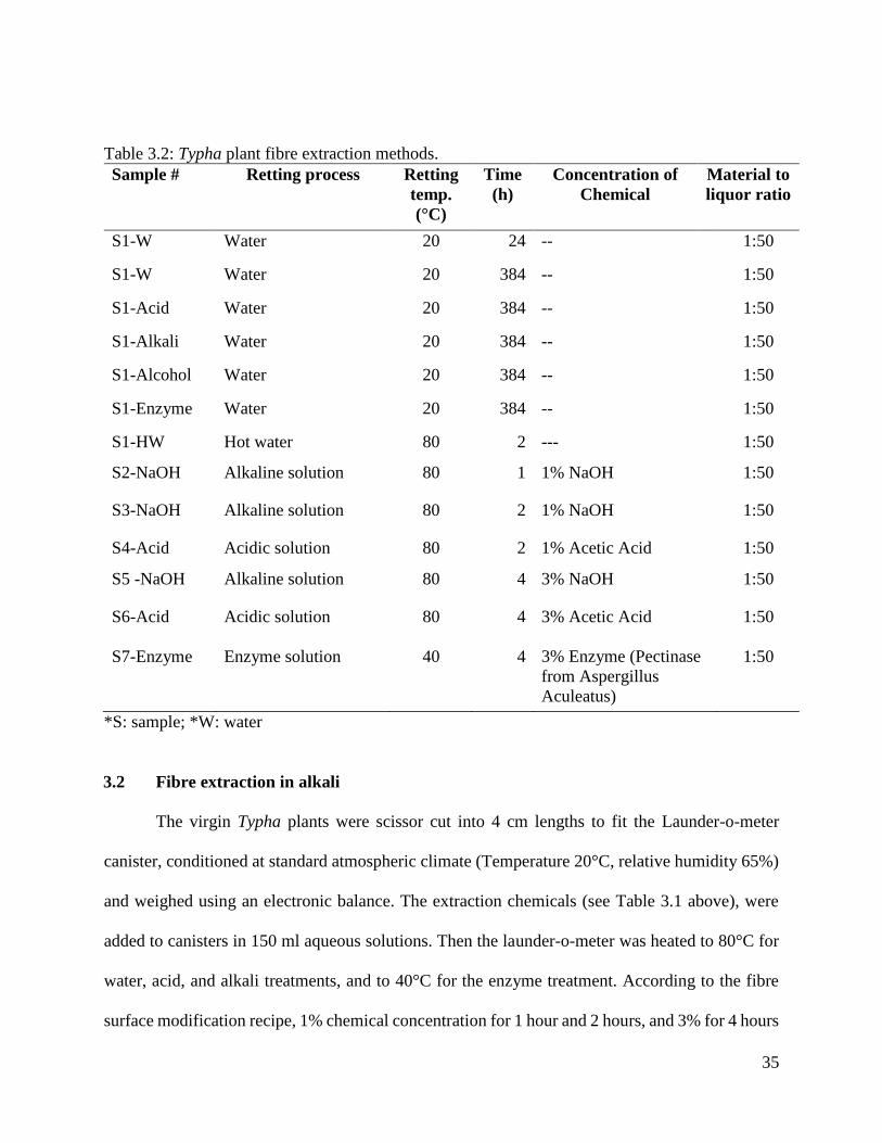
35

Table 3.2: Typha plant fibre extraction methods.

Sample # Retting process Retting

temp.

(°C)

Time

(h)

Concentration of

Chemical

Material to

liquor ratio

S1-W Water 20 24 -- 1:50

S1-W Water 20 384 -- 1:50

S1-Acid Water 20 384 -- 1:50

S1-Alkali Water 20 384 -- 1:50

S1-Alcohol Water 20 384 -- 1:50

S1-Enzyme Water 20 384 -- 1:50

S1-HW Hot water 80 2 --- 1:50

S2-NaOH Alkaline solution 80 1 1% NaOH 1:50

S3-NaOH Alkaline solution 80 2 1% NaOH 1:50

S4-Acid Acidic solution 80 2 1% Acetic Acid 1:50

S5 -NaOH Alkaline solution 80 4 3% NaOH 1:50

S6-Acid Acidic solution 80 4 3% Acetic Acid 1:50

S7-Enzyme Enzyme solution 40 4 3% Enzyme (Pectinase

from Aspergillus

Aculeatus)

1:50

*S: sample; *W: water

3.2 Fibre extraction in alkali

The virgin Typha plants were scissor cut into 4 cm lengths to fit the Launder-o-meter

canister, conditioned at standard atmospheric climate (Temperature 20°C, relative humidity 65%)

and weighed using an electronic balance. The extraction chemicals (see Table 3.1 above), were

added to canisters in 150 ml aqueous solutions. Then the launder-o-meter was heated to 80°C for

water, acid, and alkali treatments, and to 40°C for the enzyme treatment. According to the fibre

surface modification recipe, 1% chemical concentration for 1 hour and 2 hours, and 3% for 4 hours

36

was used as a trial of various times and temperature, to find the best fibre extraction efficiency,

absorbency and dye take up of the resultant materials.

After treatment, it was observed that the fibre bundles were clustered, so the individual

fibres were separated manually. Five minutes washing with distilled tap water neutralized the

treated fibres. Subsequently, the samples were dried and reweighed to calculate the weight loss

and the yield percentages. At the end of this process, the fibres were conditioned at standard

atmospheric conditions (temperature 20°C and relative humidity 65%).

Based on the first experiment, it was determined the alkali medium treatment worked more

efficiently than the others. In the second phase, a different alkali, potassium hydroxide (KOH),

was used to compare the fibre extraction efficiency to the sodium hydroxide (NaOH) treatment

used in the first experiment. Each experiments was conducted four times for four types of samples

(for example S8-K1-MS, S8-K1-HS, S8-K1-SS, and S8-K1-NS) with same concentrations of

alkali, and temperatures were replicated, and times were increased to determine the effect on fibre

extraction efficiency (see Table 3.3).

Table 3.3: Experimental conditions (3% chemical concentration and 1:50 liquor ratio) for

chemical treatment of Typha fibres.

Sample# Treatment time

(h)

Retting temp.

(°C)

S8-K1 2 80

S8-K2 4 80

S8-K3 6 80

S8-K4 8 80

*S: sample; *KOH: Potassium hydroxide

To determine the significance of temperature on fibre extraction, samples were treated with

KOH in 150 ml aqueous solution and run in the Launder-o-meter at a temperature of 95°C for

times of 2, 4, 6, and 8 hours, and the resulting yield percentage was calculated.

37

Table 3.4: Experimental conditions (3% chemical concentration and 1:50 liquor ratio) for KOH

treatment of Typha fibres.


(h)

Retting temp.

(°C)

S9-K5 2 95

S9-K6 4 95

S9-K7 6 95

S9-K8 8 95

*S: sample; *KOH: Potassium hydroxide

Another fibre extraction method using lithium hydroxide (LiOH) in 3% concentration

solution was tested to see if it would perform better in the extraction and separation of the fibres.

The samples were treated in the solution (Table 3.5) in the launder-o-meter using different time

cycles.

Table 3.5: Experimental conditions (3% chemical concentration and 1:50 liquor ratio) for LiOH

treatment of Typha fibres.


(h)

Retting temp.

(°C)

S10-L1 2 80

S10-L2 4 80

S10-L3 6 80

S10-L4 8 80

*S: sample; *L: Lithium hydroxide

3.3 Fibre Characterization

In the table below, methods which were used in Typha fibre properties characterization are

described (Table 3.6).

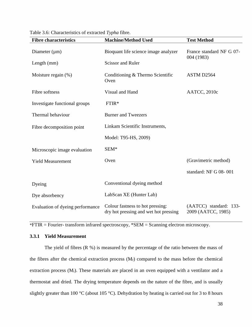
38

Table 3.6: Characteristics of extracted Typha fibre.

*FTIR = Fourier- transform infrared spectroscopy, *SEM = Scanning electron microscopy.

3.3.1 Yield Measurement

The yield of fibres (R %) is measured by the percentage of the ratio between the mass of

the fibres after the chemical extraction process (Mf) compared to the mass before the chemical

extraction process (Mi). These materials are placed in an oven equipped with a ventilator and a

thermostat and dried. The drying temperature depends on the nature of the fibre, and is usually

slightly greater than 100 °C (about 105 °C). Dehydration by heating is carried out for 3 to 8 hours

Fibre characteristics Machine/Method Used Test Method

Diameter (µm)

Bioquant life science image analyzer

France standard NF G 07-

004 (1983)

Length (mm) Scissor and Ruler

Moisture regain (%) Conditioning & Thermo Scientific

Oven

ASTM D2564

Fibre softness Visual and Hand AATCC, 2010c

Investigate functional groups FTIR*

Thermal behaviour Burner and Tweezers

Fibre decomposition point Linkam Scientific Instruments,

Model: T95-HS, 2009)

Microscopic image evaluation SEM*

Yield Measurement Oven (Gravimetric method)

standard: NF G 08- 001

Dyeing Conventional dyeing method

Dye absorbency LabScan XE (Hunter Lab)

Evaluation of dyeing performance

Colour fastness to hot pressing:

dry hot pressing and wet hot pressing

(AATCC) standard: 133-

2009 (AATCC, 1985)

39

until a dry or almost dry constant weight (Mf) is reached. The gravimetric method was used with

the following standard: NF G 08- 001, to calculate fibre yield (%).

R (%) = (Mf /Mi) *100 (Eq. 1)

3.3.2 Statistical analysis of Typha fibre length

The analysis can be considered a completely randomized design in the selection of

individual fibres from fibre bundles, and the two treatments selected from the 12 treatments shown

in Appendix III.

For Treatment 1: S8-K4-MS and Treatment 2: S10-L4-MS, the model can be expressed as shown

in (Eq. 1).

yij = + hi + eij (Eq.2)

In Eq. 1:

yij = Fibre length of jth observation on ith treatment.

= Population mean.

hi = Effect of ith treatment, i = 1 to 2 and j= 1 to 15;

eij = error deviation.

From this model, the null hypothesis is, hO: hi=hi - Effects are same; the alternative hypothesis is

ha: hi hi - Effects are different;

3.3.3 Diameter measurement

The diameter of the fibre was determined using a Bioquant Analyzer, which was connected

to a computer, a projection microscope and a camera. The Typha fibre was prepared on a glass

slide and observed using 40x magnifications. Computer software was used to calculate the fibre

40

diameter. The same method was used to determine the diameter of Typha fibre samples from fibre

bundles along the length of each fibre. Statistical analysis was done to compare the fibre diameter

of Typha, Cotton and wool. To determine diameter, France standard NF G 07- 004 (1983) and unit

was considered as micrometer (µm). For this diameter comparison, 10 single fibre samples were

chosen and 10 diameter readings from each fibre, which are shown in 5.4 (a), 5.4 (b) and 5.4 (c),

were taken and the average diameter of 10 readings (fibre #1 – fibre# 10) with the standard

deviation is calculated (Table 5.3(a)). For comparison, two of the most commonly used fibres,

Cotton and wool, were also measured. The individual reading for 100 diameter values are given in

Appendix III.

3.3.4 Softness Measurement

The softness of Typha fibre was evaluated by a survey method, according to AATCC

evaluation procedure 5 (AATCC, 2010a) standard, which results in a numeric scale for the purpose

of softness grading. Fibres bundles are taped to a piece of cardboard and placed into small polybags

(2 x 2 inches), and evaluators graded it for softness in a range of 1- 5. The lowest softness (in terms

of easy fibre separation and touch feeling) is given a rating of 1, and 5 indicates the highest softness

(in terms of easy fibre separation and touch feeling method). Softness data for textile fibre Cotton,

silk, wool, nylon, acrylic, polyester, linum, brassica and Typha (virgin) fibre and modified Typha

fibre were used to develop the test method for this evaluation. The common textile fibres were

used to compare the standardization with sample fibres in Table 5.23.

3.3.5 Moisture regain (%) measurements

The moisture regain of Typha fibre was measured according to the ASTM D 1776- 4 (2008).

For this experiment, the humidity chamber was used at the University Manitoba grain storage

building. Before starting the moisture regain test, all samples were oven dried at 105C for eight

41

hours. Then the samples were held in a humidity chamber using a range of relative humidity and

temperatures of 50%, 59%, 61% and 65% RH and 20°C, 21°C, 24.9°C and 25°C respectively, with

various conditioning times. The moisture regain was calculated as the ratio of the amount of water

absorbed to the dry weight of the sample.

Moisture Regain (%) =W

O x 100% (Eq. 3)

Where: W= Weight of water in the fibres (g);

O= Oven dry fibre weight (g)

3.3.6 Infrared (IR) spectrum study

Sample preparation

IR spectroscopy helps to determine the functional groups of a fibre through

electromagnetic wavelengths (relatively sharp absorption bands and transmission energy source)

that are displayed on a monitor. Since Typha fibre is considered a lignocellulosic fibre having a

heterogeneous structure (Sana et al., 2014), IR spectroscopy was the best application to determine

the functional groups and chemical structure for the Typha fibres.

IR spectra measurement

Samples were prepared, placed in the sample holder of the instrument, and the spectra were

recorded over the range of wavelengths between 500–4000 cm-1.

3.3.7 Thermal Analysis

Burning behaviour

To compare the burning characteristics of Typha fibre to Cotton and polyester fibres, the

most common test is the burn-test-response method. In this experiment, tweezers hold the Typha

Cotton and polyester fibre clusters, the fibres are slowly brought toward the flame of a Bunsen

42

burner at 45° angle, and the reaction on approach to the flame is observed. Further, the burning

behaviour (while in the flame) and the reaction following removal from the flame are also

observed.

Decomposition temperature

During end use application, fibres go through various processes for dyeing or other high

temperature manufacturing and laundering procedures, so it is important to know the thermal

decomposition temperature to determine the ability to withstand high temperature. To measure

typha fibre thermal properties, a decomposing point analyzer was used: Linkam Scientific

Instruments, Model: T95-HS, 2009) combined with an imaging station (Linkam Scientific

Instrument, UK). The fibre bundle specimens were placed in a glass slide and the temperature was

raised at a set rate to a maximum temperature in the analyzer. The decomposition temperature was

determined by the visual analysis of the colour change on the sample displayed on the monitor

(Brand: Dynax, Model: DX- 22L 150A11, Made: USA). The decomposition points of Typha plant,

Typha fibres and Cotton samples were determined.

3.3.8 Scanning electron microscopy (SEM)

A scanning electron microscope (SEM), located at Manitoba Institute for Material (MIM)

at the University of Manitoba, was used to examine the Typha fibre surface and cross-section.

Samples were prepared from 3% KOH treated fibre (Sample 1), 3% LiOH treated fibre (Sample

2), and untreated Typha plant (Sample 3), with and without gold coating, and mounted on the SEM

stub for examination. Morphologic details were collected with ETD (Everhart-Thornley detector)

in HiVac at low pressure for coated Typha samples, and LFD (large Detector Field) LoVac mode

at high pressure for uncoated Typha samples, Concentric Backscattered Electron (BSE) Detector

43

(CBS) in Hi and LoVac mode at high pressure for Typha samples. The SEM was used for imaging

at different magnifications from low to high (100x to 12000x) for context.

3.3.9 Typha fibre dyeing with reactive dyes

Natural fibres have the ability to absorb dye materials. In order to find out the dyeability

of Typha fibre an exhaustion dyeing technique was used. Seven hundred (700ml) liquor (dye

solution) of reactive blue 4 in the ratio of 1:700 was prepared in a beaker at room temperature and

separated into 7–100ml beakers. To each beaker was added 2.0 gram sequestering agent

Ethylenediaminetetraacetic acid (EDTA) to deactivate metal ions, and 0.5 gram non-ionic

surfactant was added as a wetting agent. Each of the alkali treated fibres S5-NaOH, S8-K2, S10-

L2, S8-K3, S10-L1, S9-K5, and Cotton were immersed into a prepared beaker, and the beakers

were placed in a Corning PC-400 hotplate, and heated to 35˚C. After 5 minutes at this temperature,

a dosing of 2.5 grams glauber salt (Na2SO4·10H20) and 1.5 gram soda ash (Na2CO3) was added

for dyeing fixation; heating was raised to 60˚C and held for 10 minutes. A further 2.5 grams salt

(NaCl) and 1.5 gram soda ash were added to each beaker and heating continued at 60˚C for a

further 45 minutes.

During the test, the dyeing process curve was followed. Dye molecules adsorption (%)

increases rapidly during the first 5 to 10 minutes, called the primary exhaustion. Alkali in dye bath

helps to increase the dye uptake and as the dye particles begin to react with the hydroxyl groups

of the Typha fibre, more reactive dye is absorbed from the bath. Alkali is added, and the reaction

continues slowly until the equilibrium state (secondary exhaustion) is reached at ~ 60 min. For

better colourfastness, the post-treatment process is very important. During the post-treatment

process, a hot wash confirms that fibre samples are totally free from unfixed dyes. Then the

samples are immersed in 100 ml water with 10ml highly concentrated (50% v/v) hydrochloric acid

44

(HCl) for 15 minutes at 60˚C to neutralize additional salts and alkalis, rinsed in cold water and

dried at room temperature for 24 hours.

Figure 3.2: Dyeing process curve.

3.3.10 Colour differences of dyed fibres

In order to find the colour differences of dyed material, it is important to know the dyeing

absorbency of the dyed fibres. The computer-controlled LabScan XE (Hunter Lab)

spectrophotometer was used to indicate the degree of dye take-up by the samples S5-NaOH, S8-

K2, S10-L2, S8-K3, S10-L1, S9-K5, and Cotton. Optical geometry was used to measure the colour

differences between the after dyeing process liquor colours and the after-treatment dyeing liquor

colours. Following this method, the dyeing liquor was measured through the bottom of a clear

glass sample cup and the port-up orientation dyeing liquor beaker covered 1.75 inch sample cup

viewing port. During the experiment, the recommended colour scale CIE 1976 L*a*b* system and

D65 recommended illuminant were used. The Commission International d'Eclairage has

established the principle of colour measurement. The colour value is expressed in terms of colour

space L*, hue angle, and chroma values (Weatherall and Bernard Coombs, 1992). CIELAB colour

45

space is shown in the below Figure 3.3. Lightness L* is denoted in vertical axis with white (L* =

100) at the top and black (L* = 0) at the bottom. The value a* and b* axes signifies chromatic

colours. The value a* axis – when colour red represents positive values and negative for green.

Similarly, positive b* values represent yellow and blue for negative b* values.

Figure 3.3: CIELAB colour space (Weatherall & Coombs, 1992).

The colour difference (ΔE) is calculated, using coordinate geometry, as the length of the line

joining the coordinate positions: The Total colour difference (ΔE), the difference in individual

parameters of the standard and a sample are also estimated e.g. ΔL = L (sample) - L (standard).

ΔE = [(ΔL*) ² + (Δa*) ² + (Δb*) ²]1/2 (Eq. 4)

3.3.11 Evaluation of dyeing performance (colourfastness to hot pressing)

End use textile products are always subjected to some major factors including moisture,

light, heat, and abrasion during processing (Khan, 2016). Using the American Association of

Textile Chemists and Colorists (AATCC) standard: 133-2009 (AATCC, 1985), the subjective

dyeing performance (colourfastness to hot pressing) of dyed samples S10-L2, S10-L1, S8-K3, S9-

K5, S8-K2, S5-NaOH, and Cotton were evaluated to determine colour resistance of dyed fibres to

colour change, and colour transfer when subjected to hot pressing.

46

The Atlas Scorch Tester (SDL, Model M247B) containing a heating device was used to

conduct colourfastness to hot pressing evaluation using fibres that were wet, dry, and damp at 65

± 2% relative humidity and temperature 21± 1°C. For dry pressing, the samples were placed on

top of the undyed Cotton fabric (130 g/m2) /wool flannel (260 g/m2) pad and subjected to a

specific pressing temperature for 15 seconds. The heating device gave an even heat transfer to the

sample between the top plate and bottom plates. In damp pressing, a similar process was followed,

but one extra piece of undyed cloth (dimension: 12 × 4 cm) was soaked with distilled water, then

squeezed until it contained its own weight of water, placed on the top the sample, and held 15

seconds with even hot pressing. For wet pressing, the samples and an extra piece of undyed cloth

(dimension: 12 cm × 4 cm) both were wet during the pressing process. Evaluation uses a grey scale

for staining (revised 1979, 1981 by AATCC / ISO 105-A03 methods) and a grey scale for colour

change (revised 1979 by AATCC / ISO 105-A02). Grey scale is graded in 9 different grades such

as 1, 1-2, 2, 2-3, 3, 3-4, 4, 4-5 and 5, where grade 1 denotes the highest staining or colour change,

and grade 5 denotes no staining or colour change during washing (Collier & Epps, 1999).

3.3.12 Statistical analysis

Different statistical analytical techniques are employed in this current research in chapters

4.0 and 5.0. A single Factor ANOVA used, two-way ANOVA test, Fisher’s LSD and Tukey test

were considered to test the hypothesis. The test for the significance of the factor round by defining

a linear model and creating an ANOVA-Table and Post Hoc test method used for a multi-

comparison. This statistical analyses were performed with Excel-16.0 version and the SPSS

version 16.0 statistical program for Windows system (SPSS) and able to test the effect size, main

effects and interaction between individual variables, significant difference within the variables.

Differences were considered significant at p =0.05.

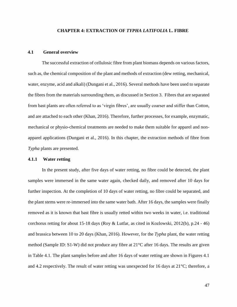
47

CHAPTER 4: EXTRACTION OF TYPHA LATIFOLIA L. FIBRE

4.1 General overview

The successful extraction of cellulosic fibre from plant biomass depends on various factors,

such as, the chemical composition of the plant and methods of extraction (dew retting, mechanical,

water, enzyme, acid and alkali) (Dungani et al., 2016). Several methods have been used to separate

the fibres from the materials surrounding them, as discussed in Section 3. Fibres that are separated

from bast plants are often referred to as ‘virgin fibres’, are usually coarser and stiffer than Cotton,

and are attached to each other (Khan, 2016). Therefore, further processes, for example, enzymatic,

mechanical or physio-chemical treatments are needed to make them suitable for apparel and non-

apparel applications (Dungani et al., 2016). In this chapter, the extraction methods of fibre from

Typha plants are presented.

4.1.1 Water retting

In the present study, after five days of water retting, no fibre could be detected, the plant

samples were immersed in the same water again, checked daily, and removed after 10 days for

further inspection. At the completion of 10 days of water retting, no fibre could be separated, and

the plant stems were re-immersed into the same water bath. After 16 days, the samples were finally

removed as it is known that bast fibre is usually retted within two weeks in water, i.e. traditional

corchorus retting for about 15-18 days (Roy & Lutfar, as cited in Kozlowski, 2012(b), p.24 - 46)

and brassica between 10 to 20 days (Khan, 2016). However, for the Typha plant, the water retting

method (Sample ID: S1-W) did not produce any fibre at 21°C after 16 days. The results are given

in Table 4.1. The plant samples before and after 16 days of water retting are shown in Figures 4.1

and 4.2 respectively. The result of water retting was unexpected for 16 days at 21°C; therefore, a

48

longer retting time of up to 90 days at room temperature (Sample ID: S3-W; Figure 4.4) and higher

temperature of 80°C for up to 6 hours (Sample: S2-W; Figure 4.3) were investigated. No Typha

fibre could be obtained from these two retting processes (Table 4.1).

It can be seen in Table 4.1 that some weight loss occurred during the attempted water

retting. To identify the source of the weight loss, fresh plant samples were weighed after drying in

the oven for 24 hours at 105°C and found to be 4.8 gram. These plant samples were then washed

in water to remove the dirt, mud and other foreign materials, again oven dried for 24 hours at

105°C, and reweighed. The washed samples weighed 4.5 gram. The loss in weight of the washed

samples explained some of the weight loss during water retting. Since no Typha fibre was obtained

after 90 days of water retting at room temperature and 6 hours’ treatment at 80°C, it was decided

to investigate chemical and enzymatic retting methods in order to extract fibre from the Typha

plants. The Typha demonstrated good resistance to extraction of starch, and it is hard to break the

Typha cell walls (Fahlgren, 2017). Water retting cannot extract fibre from the Typha plant because

the Typha plants grow in shallow waters, waterlogged ponds, ditches, and wetlands (Lidman, as

cited by Fahlgren, 2017, p.7). Further, it is known that 94% of Typha can survive in 2.4% saline

water in field conditions (Jesus et al., as cited in Fahlgren, 2017). Additionally, previous research

has found that Typha is considered a highly water tolerant plant (ACT, 2013) compared to other bast

fibres such as corchorus that do not tolerate a waterlogged environment (Roy & Lutfar, as cited by

Kozlowski, 2012b, p. 27), and have a very high resistance to mold growth (Krus et al., 2014).

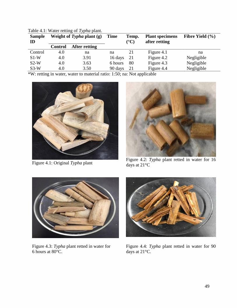
49

Table 4.1: Water retting of Typha plant.

Sample

ID

Weight of Typha plant (g) Time Temp.

(°C)

Plant specimens

after retting

Fibre Yield (%)

Control After retting

Control 4.0 na na 21 Figure 4.1 na

S1-W 4.0 3.91 16 days 21 Figure 4.2 Negligible

S2-W 4.0 3.63 6 hours 80 Figure 4.3 Negligible

S3-W 4.0 3.50 90 days 21 Figure 4.4 Negligible

*W: retting in water, water to material ratio: 1:50; na: Not applicable

Figure 4.1: Original Typha plant

Figure 4.2: Typha plant retted in water for 16

days at 21°C

Figure 4.3: Typha plant retted in water for

6 hours at 80°C.

Figure 4.4: Typha plant retted in water for 90

days at 21°C.

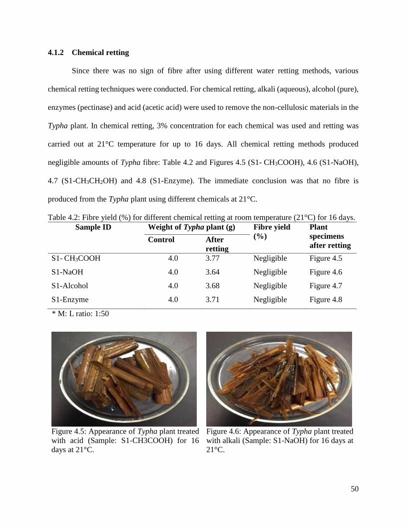
50

4.1.2 Chemical retting

Since there was no sign of fibre after using different water retting methods, various

chemical retting techniques were conducted. For chemical retting, alkali (aqueous), alcohol (pure),

enzymes (pectinase) and acid (acetic acid) were used to remove the non-cellulosic materials in the

Typha plant. In chemical retting, 3% concentration for each chemical was used and retting was

carried out at 21°C temperature for up to 16 days. All chemical retting methods produced

negligible amounts of Typha fibre: Table 4.2 and Figures 4.5 (S1- CH3COOH), 4.6 (S1-NaOH),

4.7 (S1-CH3CH2OH) and 4.8 (S1-Enzyme). The immediate conclusion was that no fibre is

produced from the Typha plant using different chemicals at 21°C.

Table 4.2: Fibre yield (%) for different chemical retting at room temperature (21°C) for 16 days.

Sample ID Weight of Typha plant (g) Fibre yield

(%)

Plant

specimens

after retting Control After

retting

S1- CH3COOH 4.0 3.77 Negligible Figure 4.5

S1-NaOH 4.0 3.64 Negligible Figure 4.6

S1-Alcohol 4.0 3.68 Negligible Figure 4.7

S1-Enzyme 4.0 3.71 Negligible Figure 4.8

* M: L ratio: 1:50

Figure 4.5: Appearance of Typha plant treated

with acid (Sample: S1-CH3COOH) for 16

days at 21°C.


with alkali (Sample: S1-NaOH) for 16 days at

21°C.

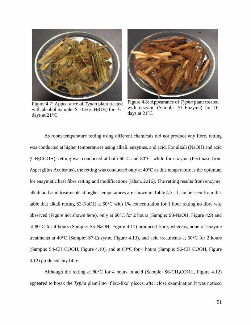
51


with alcohol Sample: S1-CH3CH2OH) for 16

days at 21°C


with enzyme (Sample: S1-Enzyme) for 16

days at 21°C

As room temperature retting using different chemicals did not produce any fibre, retting

was conducted at higher temperatures using alkali, enzymes, and acid. For alkali (NaOH) and acid

(CH3COOH), retting was conducted at both 60°C and 80°C, while for enzyme (Pectinase from

Aspergillus Aculeatus), the retting was conducted only at 40°C as this temperature is the optimum

for enzymatic bast fibre retting and modifications (Khan, 2016). The retting results from enzyme,

alkali and acid treatments at higher temperatures are shown in Table 4.3. It can be seen from this

table that alkali retting S2-NaOH at 60°C with 1% concentration for 1 hour retting no fibre was

observed (Figure not shown here), only at 60°C for 2 hours (Sample: S3-NaOH, Figure 4.9) and

at 80°C for 4 hours (Sample: S5-NaOH, Figure 4.11) produced fibre; whereas, none of enzyme

treatments at 40°C (Sample: S7-Enzyme, Figure 4.13), and acid treatments at 60°C for 2 hours

(Sample: S4-CH3COOH, Figure 4.10), and at 80°C for 4 hours (Sample: S6-CH3COOH, Figure

4.12) produced any fibre.

Although the retting at 80°C for 4 hours in acid (Sample: S6-CH3COOH, Figure 4.12)

appeared to break the Typha plant into ‘fibre-like’ pieces, after close examination it was noticed

52

that most of these pieces were ‘plant flakes’ (flake width ≈ 68 µm – 2 mm) and attached to each

other. In order to find out whether a longer treatment time in acid might yield fibre, the Typha

plant was treated at 80°C for 8 hours; however, no fibre could be seen (Figure 4.14). Further, no

fibre was found when the Typha plant treated in acetic acid for 20 days either at room temperature

or in sulphuric acid for 60 days at room temperature (Figure not shown here).

The fibre was found from NaOH retting depended on the retting temperature. It is worth

mentioning here that, unlike other bast fibre, where, fibre is extracted from the outer layer of the

plant, for the Typha plant, the bulk of the plant could be transformed into fibre, as discussed in

Section 4.3.1. A few ‘flakes’ (bark) could be seen in some of the fibre samples, (Figures 4.9, 4.12

and 4.13). The sources of this barks are discussed in Section 4.3.1. Further, the fibre yield (%) for

Typha plant was much higher for alkaline treated samples (Table 4.3) than for brassica, linum and

cannabis where the fibre yield range is between 10 - 15% (Khan, 2016).

It is known that natural fibre can be treated with up to 28% alkali to improve the fibre

adhesion for composite applications without a significant reduction in strength (Naveen et al.,

2015). Since fibre can be obtained using NaOH, and no damage of the fibre was reported when

using up to 28% NaOH (Naveen et al., 2015), Typha plants were immersed in 10% NaOH solution

at room temperature for 30 days. However, no fibre could be obtained for this experimental

condition. Therefore, it is concluded that room temperature is not suitable for fibre extraction from

Typha using alkali and no further experiments were carried out at room temperature.

53

Table 4.3: Effect of different chemicals treatment in fibre extraction

Sample ID Time

(hour)

Conc.

(%)

Temp.

(°C)

Weight of the Typha

plant (g)

Fibre obtained

from

chemical

retting

Plant

specimens

after

retting

(Shown in

Figure)

Before

treatment

After

treatment

S2-NaOH 1 1.0 60 4.0 3.73 No ---

S3-NaOH 2 1.0 60 4.0 3.14 Yes 4.9

S4- CH3COOH 2 1.0 60 4.0 3.62 No 4.10

S5 -NaOH 4 3.0 80 4.0 2.24 Yes 4.11

S6- CH3COOH 4 3.0 80 4.0 3.47 No 4.12

S7-Enzyme 4 3.0 40 4.0 3.68 No 4.13

S7- CH3COOH 8 3.0 80 2.8 2.77 No 4.14

* S: sample; Enzyme: Pectinase from Aspergillus Aculeatus; M: L-1:50.


with alkali (Sample: S3-NaOH) for

2h/1%/60°C


with alkali (Sample: S4-CH3COOH) for

2h/1%/60°C

Figure 4.11: Appearance of Typha plant

treated with alkali (Sample: S5-NaOH) for

4h/3%/80°C


with acid (Sample: S6- CH3COOH) for

4h/3%/80°C

54


treated with acid (Sample: S7- CH3COOH) for

8h/3%/80°C


treated with Enzyme (Sample: S7-Enzyme) for

4h/3%/40°C

4.2 Effect of various alkalis on fibre yield

4.2.1 Fibre yield (%) from mixed plants

Since Typha fibre was obtained using aqueous NaOH solution, two other alkalis (KOH and

LiOH) were used for fibre extraction from mixed or unknown Typha plants. The term ‘mixed stem’

plants will be discussed later in the section. The fibre yield (%) with experimental conditions for

these two alkalis is shown in Table 4.4. As with the NaOH treatment, fibre was obtained under all

experimental conditions using both KOH and LiOH [Figures 4.15 (a) - 4.27 (a)].

Table 4.4 shows the effect of time on Typha fibre yield (%), where it can be seen that the

fibre yield (%) decreases with the increase in treatment time. As seen in Table 4.4, at 80°C in KOH

and LiOH the fibre yields were 50.0% (Sample: S8-K1-MS, Figure 4.15), 55% (Sample: S8-K2-

MS, Figure 4.16), 35% (Sample: S8-K3-MS, Figure 4.17), 15% (Sample: S8-K4-MS, Figure 4.18)

and 66% (S10-L1-MS,Figure 4.23 (a)), 54% (S10-L2-MS, Figure 4.24 (a)), 56% (S10-L3-MS,

Figure 4.25 (a)) and 53% (S10-L4-MS, Figure 4.26 (a)); after 2, 4, 6 and 8 hours respectively.

However, a similar trend of decreasing yield with treatment time was not obtained for

samples treated at 95°C in KOH solution fibre yield was 20% (Sample: S9-K5-MS, Figure 4.19),

55

25% (Sample: S9-K6-MS, Figure 4.20), 20% (Sample S9-K7-MS, Figure 4.21) and 34% (Sample:

S9-K7-MS, Figure 4.22).

It was found using similar treatment conditions in KOH at 95°C, the fibre yield was much

lower than KOH at 80°C for all treatment hours, except the 8 hours treated sample (Table 4.4). It

is worth noting here that for the equivalent treatment conditions, the yield (%) using LiOH is much

higher than the KOH, particularly after 6 and 8-hours’ treatment. For example, after 6 hours’

treatment at 80°C, KOH treatment produced 35% fibre [S8-K3-MS, Figure 4.17(a)], whereas the

LiOH produced 56% fibre [S10-L3-MS, Figure 4.25(a)], and after 8 hours of treatment, KOH

treatment produced 15% fibre [S8-K4-MS, Figure 4.18 (a)] compared to 53% fibre [S10-L4-MS,

Figure 4.26(a)] produced in LiOH.

Table 4.4: Fibre yield (%) from mixed stem plants at 3% concentration in KOH (80°C & 95°C)

and LiOH (80°C) solution for different temperature.

Alkali Sample ID Temperature

(°C)

Time

(hours)

Yield

(%)

Resultant fibre

(Shown in Figure)

KOH S8-K1-MS 80 2 50.00 4.15 (a)

KOH S8-K2-MS 80 4 55.00 4.16 (a)

KOH S8-K3-MS 80 6 35.00 4.17 (a)

KOH S8-K4-MS 80 8 15.00 4.18 (a)

KOH S9-K5-MS 95 2 20.00 4.19 (a)

KOH S9-K6-MS 95 4 25.00 4.20 (a)

KOH S9-K7-MS 95 6 20.00 4.21 (a)

KOH S9-K8-MS 95 8 34.00 4.22 (a)

LiOH S10-L1-MS 80 2 66.00 4.23 (a)

LiOH S10-L2-MS 80 4 54.00 4.24 (a)

LiOH S10-L3-MS 80 6 56.00 4.25 (a)

LiOH S10-L4-MS 80 8 53.00 4.26 (a)

56

Figure 4.15 (a): Appearance of Typha plant

treated with alkali (Sample: S8-K1-MS) for

2h at 80°C



2h at 95°C


treated with alkali (Sample: S9-K6-MS) for 4h

at 95°C



8h at 95°C

Figure 3.19(C): Typha latifolia L. fibre

treated with alkali (Sample ID: S9-K5) for

2h/3%/95 °C (NS)



4h at 80°C



6h at 80°C

57


treated with LiOH (Sample: S10-L3-MS) for

6h at 80°C



2h at 80°C



6h at 95°C


treated with LiOH (Sample: S9-K8-MS) for

8h at 80°C



4h at 80°C



8h at 80°C

58

It seems that there is no clear trend in fibre yield (%) with treatment time and temperature

when treated in KOH and LiOH. The investigation of the yield variations shown in Table 4.4,

revealed that there were three types of plant used for the study and these plant samples are termed

‘mixed samples: (a) plants with a hard stem, (b) plants with a soft stem, and (c) plants with no

stem (leaves only plant). While the detailed study of the plants is beyond the scope of the current

study, a brief description of these three plant components is given in Section 4.2.2 and the fibre

yield (%) from these plants is given in Section 4.3.1 Also, it is worth mentioning here that some

of the fibre samples contain ‘flake/bark’ like materials as shown in [Figures 4.15 (a), 4.18 (a), 4.19

(a) and 4.24 (a)].

Figure 4.15 (a): Flake/bark material exists in

(Sample: S8-K1-MS).


(Sample: S8-K4-MS).


(Sample: S9-K5-MS).


(Sample: S10-L2-MS).

59

4.2.2 Fibre yield (%) on hard stem (HS), soft stem (SS) and no stem (NS) plants

Tables 4.5, 4.6 and 4.7 exhibited the fibre yield (%) from hard stem (HS), soft stem (SS)

and no stem (only leaves plant) (NS) plants in KOH (80°C and 95°C) and LiOH at 80°C for

different treatment times. Similar to mixed plants, fibre was obtained from all three plants as shown

in Figures 4.15 (b) - 4.26 (b) for hard stem, Figures 4.15 (c) - 4.26 (c) for soft stem and Figures

4.15 (d) - 4.26 (d) for no stem plants which are given in Appendix I. Again, no clear trend can be

seen between fibre yield (%), treatment time and treatment temperature, although at 95°C in KOH

and at 80 °C in LiOH, there was tendency for decreasing yield (%) with the treatment time for the

three plants, while at 80°C in KOH, no such trend was observed. In general, it can be stated that

the yield (%) varies between 50-30, 55-30 and 47-25 for the hard, soft and no stem respectively.

An important observation was made in the fibre from hard and soft plants: these fibres contain

flakes [Figures 4.17 (b), 4.19 (b), 4.20 (b) 4.23 (b) 4.25 (b) and 4.26 (b) are located in Appendix

I], no such flakes could be seen in the fibres that were obtained from no stem plants. Therefore,

some components in hard and soft plants may have been responsible in contributing flakes in the

fibres, as discussed in Section 4.3.

Table 4.5: Effect of time on the hard stems plant fibres yield (%) at 3% concentration in KOH

(80°C & 95°C) and LiOH (80°C) solution for different temperature.

Alkali Sample ID Temperature Time Yield% Resultant fibre (Shown in Figure)

KOH S8-K1-HS 80 2 50.90 4.15 (b)

KOH S8-K2-HS 80 4 38.52 4.16 (b)

KOH S8-K3-HS 80 6 36.24 4.17 (b)

KOH S8-K4-HS 80 8 41.27 4.18 (b)

KOH S9-K5-HS 95 2 44.00 4.19 (b)

KOH S9-K6-HS 95 4 41.00 4.20 (b)

KOH S9-K7-HS 95 6 35.00 4.21 (b)

KOH S9-K8-HS 95 8 32.00 4.22 (b)

LiOH S10-L1-HS 80 2 35.00 4.23 (b)

LiOH S10-L2-HS 80 4 28.00 4.24 (b)

LiOH S10-L3-HS 80 6 29.00 4.25 (b)

LiOH S10-L4-HS 80 8 30.00 4.26 (b)

Figures 4.15 (b) – 4.26 (b) located in Appendix I

60

Table 4.6: Effect of time on the soft stems plants fibres yield (%) at 3% concentration in KOH

(80°C & 95°C) and LiOH (80°C) solution for different temperature.


(°C)

Time

(hours)

Yield% Resultant fibre

(Shown in Figure)

KOH S8-K1-SS 80 2 31.50 4.15 (c)

KOH S8-K2-SS 80 4 33.60 4.16 (c)

KOH S8-K3-SS 80 6 42.00 4.17 (c)

KOH S8-K4-SS 80 8 32.14 4.18 (c)

KOH S9-K5-SS 95 2 55.49 4.19 (c)

KOH S9-K6-SS 95 4 42.37 4.20 (c)

KOH S9-K7-SS 95 6 33.76 4.21 (c)

KOH S9-K8-SS 95 8 39.57 4.22 (c)

LiOH S10-L1-SS 80 2 39.53 4.23 (c)

LiOH S10-L2-SS 80 4 36.63 4.24 (c)

LiOH S10-L3-SS 80 6 37.10 4.25 (c)

LiOH S10-L4-SS 80 8 39.94 4.26 (c)

Figures 4.15 (c) – 4.26 (c) located in Appendix I

Table 4.7: Effect of time on the no stems (only leaves plant) plants fibres yield (%) at 3%

concentration in KOH (80°C & 95°C) and LiOH (80°C) solution for different temperature.


(°C)

Time

(hours)

Yield% Resultant fibre

(Shown in Figure)

KOH S8-K1-NS 80 2 45.43 4.15 (d)

KOH S8-K2-NS 80 4 35.13 4.16 (d)

KOH S8-K3-NS 80 6 41.34 4.17 (d)

KOH S8-K4-NS 80 8 32.04 4.18 (d)

KOH S9-K5-NS 95 2 35.03 4.19 (d)

KOH S9-K6-NS 95 4 35.27 4.20 (d)

KOH S9-K7-NS 95 6 32.23 4.21 (d)

KOH S9-K8-NS 95 8 31.31 4.22 (d)

LiOH S10-L1-NS 80 2 46.01 4.23 (d)

LiOH S10-L2-NS 80 4 33.24 4.24 (d)

LiOH S10-L3-NS 80 6 31.52 4.25 (d)

LiOH S10-L4-NS 80 8 27.69 4.26 (d)

Figures 4.15 (d) – 4.26 (d) located in Appendix I.

4.2.3 Data analysis

The statistical analysis was conducted to determine the variation in yield (%) among the

treatment hours (2, 4, 6 and 8), treatment temperature (80°C in KOH, 80°C in LiOH and 95°C in

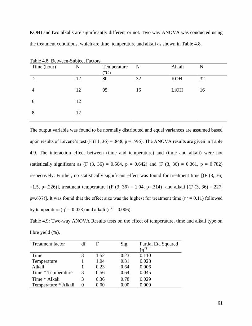
61

KOH) and two alkalis are significantly different or not. Two way ANOVA was conducted using

the treatment conditions, which are time, temperature and alkali as shown in Table 4.8.

Table 4.8: Between-Subject Factors

Time (hour) N Temperature

(°C)

N Alkali N

2

12 80 32 KOH 32

4 12 95 16 LiOH 16

6

12

8

12

The output variable was found to be normally distributed and equal variances are assumed based

upon results of Levene’s test (F (11, 36) = .848, p = .596). The ANOVA results are given in Table

4.9. The interaction effect between (time and temperature) and (time and alkali) were not

statistically significant as (F (3, 36) = 0.564, p = 0.642) and (F (3, 36) = 0.361, p = 0.782)

respectively. Further, no statistically significant effect was found for treatment time [(F (3, 36)

=1.5, p=.226)], treatment temperature [(F (3, 36) = 1.04, p=.314)] and alkali [(F (3, 36) =.227,

p=.637)]. It was found that the effect size was the highest for treatment time (η2 = 0.11) followed

by temperature (η2 = 0.028) and alkali (η2 = 0.006).

Table 4.9: Two-way ANOVA Results tests on the effect of temperature, time and alkali type on

fibre yield (%).

Treatment factor df F Sig. Partial Eta Squared

(η2)

Time 3 1.52 0.23 0.110

Temperature 1 1.04 0.31 0.028

Alkali 1 0.23 0.64 0.006

Time * Temperature 3 0.56 0.64 0.045

Time * Alkali 3 0.36 0.78 0.029

Temperature * Alkali 0 0.00 0.00 0.000

62

Table 4.10: Results of Post Hoc Tests for the effect of time on yield (%)

Time

(I)

Time

(J)

LSD

2 4 0.230> p

6 0.082> p

8 S0.033< p

4 2 0.230> p

6 0.572> p

8 0.327> p

6 2 0.082> p

4 0.572> p

8 0.674> p

8 2 S0.033> p

4 0.327> p

6 0.674> p

*s=significant, p =0.05.

The LSD post hoc test was used for multiple comparison (Table 4.12) which showed that

the yield (%) is significantly different (p=0.033<0.05) between two hours (M =43.24, SD= 4.17)

and eight hours ((M=35.78, SD= 4.17).

4.3 Sources of flakes and barks in the fibre

As mentioned earlier, fibre-like pieces (plants flakes and bark) broke off the Typha stems

during the retting process. The flakes are fibre like materials found in fibre bundles from which

fibre can be separated by hand after immersing the stems in water; whereas, bark is a part of the

hard/soft woody stems. Fibre cannot be separated by hand from these stems after immersing in

water. Since the fibre yield (%) varied widely, within a fibre bundle, all Typha plants used in the

current study were analyzed for their plant morphology. It was found that three different types of

Typha plants were used:

(1) Plant with a hard wood stem – Figure 4.27(a) & 4.27(b): Cross-section with different

components.

(2) Plant with a soft stem - Figure 4.28(a) & 4.28(b): Cross-section with different

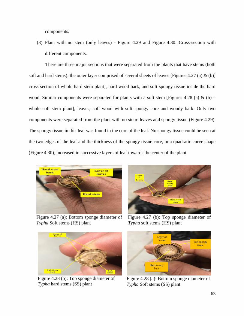
63

Figure 4.28 (b): Top sponge diameter of

Typha hard stems (SS) plant

Figure 4.28 (a): Bottom sponge diameter of

Typha Soft stems (SS) plant

components.

(3) Plant with no stem (only leaves) - Figure 4.29 and Figure 4.30: Cross-section with

different components.

There are three major sections that were separated from the plants that have stems (both

soft and hard stems): the outer layer comprised of several sheets of leaves [Figures 4.27 (a) & (b)]

cross section of whole hard stem plant], hard wood bark, and soft spongy tissue inside the hard

wood. Similar components were separated for plants with a soft stem [Figures 4.28 (a) & (b) –

whole soft stem plant], leaves, soft wood with soft spongy core and woody bark. Only two

components were separated from the plant with no stem: leaves and spongy tissue (Figure 4.29).

The spongy tissue in this leaf was found in the core of the leaf. No spongy tissue could be seen at

the two edges of the leaf and the thickness of the spongy tissue core, in a quadratic curve shape

(Figure 4.30), increased in successive layers of leaf towards the center of the plant.

Figure 4.27 (b): Top sponge diameter of

Typha soft stems (HS) plant

Figure 4.27 (a): Bottom sponge diameter of

Typha Soft stems (HS) plant

Layer of

leaves

Hard woody

bark

Soft spongy

tissue

64

Figure 4.29: Different components of Typha

plant leaves.

Figure 4.30: Quadratic curve shape of Typha

plant

Table 4.8 shows Typha plant morphology, including components and dimensions – whole

plant diameter, leaf, stem, and spongy tissue. The diameter of the no stem plant (30.4 mm) is much

higher than the hard (10.59 mm) and soft stem (16.76 mm) plants. This diameter was measured 25

mm above the bottom of the plant. Similarly, larger leaf width, which was measured 2.5 cm from

bottom, was obtained for no stem plant (leaf width: 5.1 cm) than the hard (leaf width: 3.0 cm) and

soft stem (leaf width: 4.6 cm). After removing the leaves, they could be measured for the no stem

plant; the diameter of the hard stem (bark + sponge) and soft stem (bark + sponge) plants was

found to be 5.42 ± 0.36 mm and 9.5 ± 0.97 mm respectively. As mentioned earlier, both hard and

soft stem plants as well as no stem plant leaf contained spongy tissue and diameter of the spongy

tissue was 4.41 ± 0.51 mm for hard stem and 7.69 ± 1.20 mm for the soft stem plant. The diameter

of the spongy core of the no stem leaf varies widely due to the quadratic curve shape, however,

the diameter of the widest section of the spongy core was found to be 2.2 mm.

Successive layer

of leaves

Spongy tissue inside

the leaves

65

Table 4.11: Plant morphology for hard, soft and no-stem of Typha plants with dimensions

4.2.1 Fibre extraction from various plant components of Typha plant

In order to investigate whether or not fibre can be obtained from various components of

the hard stem (HS), soft stem (SS) and no stem (NS) Typha plants, and track the sources of the

bark/flakes in the fibre bundle, alkali treatment was carried out using 3.0% KOH at 80°C. The

treatment was conducted for 8 hours, except for one component (bark – hard and soft stems) of the

plant, where treatment was conducted for up to 12 hours.

The fibre, fibre yield (%), flakes and barks in the fibre, and visual fibre characteristics from

the different component of the plants are given in Table 4.9. It can be seen from this table (also

shown in figures) that fibre can be obtained from all of the three whole plants: hard stems, soft

stems and no stems: [Figure 4.36 (a) – whole plant (SS), Figure 4.36 (b) – fibre (left) and flakes

(right)], [Figure 4.31 (a) – whole plant (HS), Figure 4.31 (b) – fibre (left) and flakes (right)], and

[Figure 4.41 (a) – whole plant (NS), Figure 4.41 (b) – fibre, no flakes]. Further, it can be seen that

only fibres from the NS whole plant are free from flakes [Figure 4.41 (b)], while flakes/barks have

Plant

type

Whole plant

diameter (mm)

Leaf Stem diameter Spongy

(Stem + bark)

Hard

stem

10.59 (25 mm

above the root)

Yes (width:

3.0 cm, 2.54

cm from

bottom)

Yes (average diameter: 5.42

± 0.36 mm)

[5.54,5.43,5.87,4.88,5.31]

Yes (inside stem)

Inner core diameter:

4.41± 0.51 mm

[4.90,4.29,3.58,4,70,4.58]

Soft

stem

16.76 (25 mm

above the root)

Yes (width:

4.6 cm, 2.54

cm from

bottom)

Yes (average diameter: 9.5

± 0.97 mm)

[9.03,11.23,9.26,9.06,8.95]

Yes (inside stem)

Average inner core

diameter: 7.69 mm ±

1.20mm

[8.44,9.14,7.81,7.03,6.06]

No

stem

30.40 (25 mm

above the root)

Yes (width:

5.1 cm, 2.54

cm from

bottom)

No Yes, (inside leaf)

Inner core diameter

(variable): 2.2 mm

66

been separated from the fibres obtained from whole soft stem (SS) plant [Figure 4.36 (b), right]

and whole hard stem (HS) plant [Figure 4.31 (b), right].

Fibres also can be obtained from the leaves of all three plants as in Figure 4.41 (b) [NS], 4.37 (b)

[SS] and 4.32 (b) [HS]. The leaves for these plants are given in Figures 4.41 (a), 4.37 (a), and 4.31

(a), respectively for NS, SS and HS plants. No flakes could be found in the fibres obtained from

the leaves. These flakes/barks might have come from bark or/and sponge in Figures 4.36 (b) and

4.31(b).

Fibres from the hard wood + spongy tissue [HS, Figure 4.33 (a)] and soft wood + spongy

tissue [SS, Figure 4.38(a)] are given in Figures 4.33 (b) and 4.38 (b) respectively. It can be seen

from these two figures [Figures 4.38 (b) and 4.33 (b)] that fibres are mixed with flakes and barks.

The flakes/barks have been separated from the fibres and shown in Figures 4.38 (c) fibres (right)

and flakes (left) and 4.33 (c) fibres (left) and flakes (right) respectively for SS and HS plants.

Woody bark [HS, Figure 4.34 (a)], [SS, Figure 4.39 (a)] and spongy tissue [HS, Figure 4.35 (a)],

[SS, Figure 4.40 (a)] were separately treated with alkali. No fibres were extracted from the woody

bark as shown in [Figures 4.34 (b) for 6 hours, 4.34 (c) for 8 hours, 4.34 (d) for 12 hours] and

[Figures 4.39 (b) for 8 hours, 4.39 (c) for 12 hours]. When spongy tissue separated from hard [4.35

(a)] and soft stem plants [4.40 (a)], and was treated in alkali, fibres could be obtained. These fibres

are shown in Figure 4.35(b) and 4.40 (b).

The immediate conclusion is that fibres could be obtained from leaves and spongy tissue and

no fibres could be obtained from bark. The sources of the flakes/bark in the fibres have now been

established.

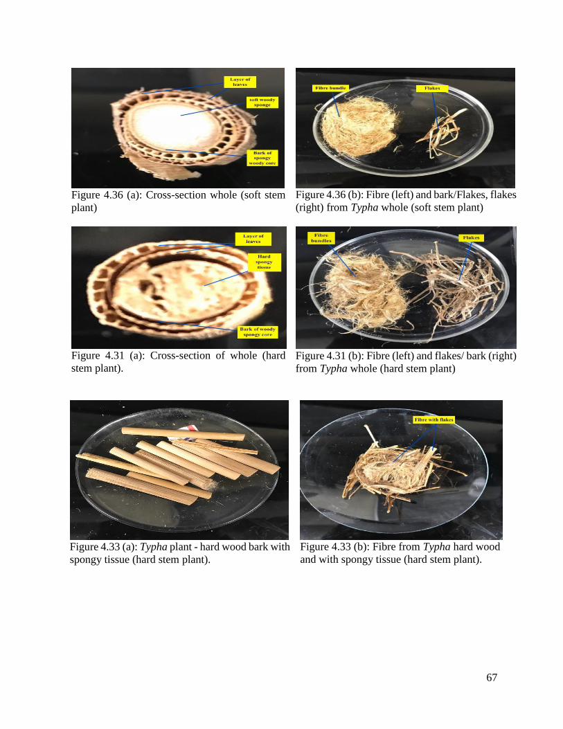
67

Figure 4.33 (a): Typha plant - hard wood bark with

spongy tissue (hard stem plant).

Figure 4.33 (b): Fibre from Typha hard wood

and with spongy tissue (hard stem plant).

Figure 4.36 (a): Cross-section whole (soft stem

plant)

Figure 4.36 (b): Fibre (left) and bark/Flakes, flakes

(right) from Typha whole (soft stem plant)

Figure 4.31 (a): Cross-section of whole (hard

stem plant). Figure 4.31 (b): Fibre (left) and flakes/ bark (right)

from Typha whole (hard stem plant)

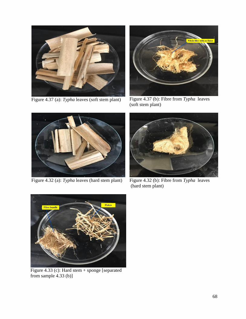
68

Figure 4.33 (c): Hard stem + sponge [separated

from sample 4.33 (b)]

Figure 4.37 (a): Typha leaves (soft stem plant)

Figure 4.37 (b): Fibre from Typha leaves

(soft stem plant)

Figure 4.32 (a): Typha leaves (hard stem plant)

Figure 4.32 (b): Fibre from Typha leaves

(hard stem plant)

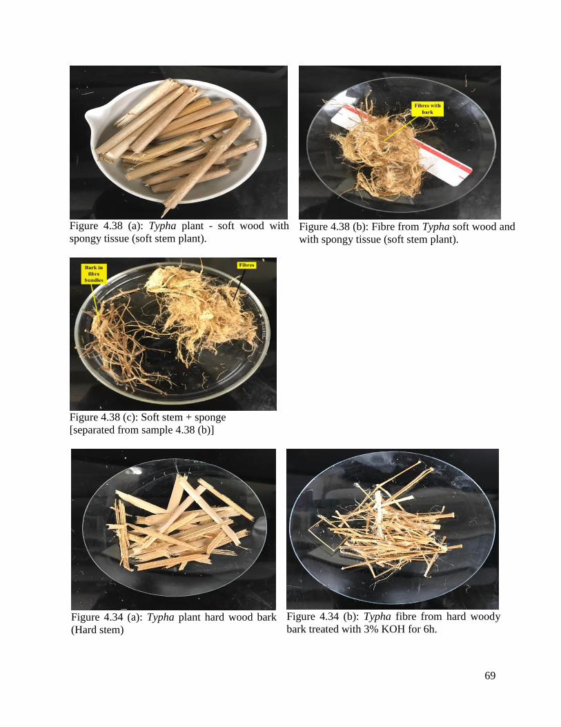
69

Figure 4.38 (a): Typha plant - soft wood with

spongy tissue (soft stem plant).

Figure 4.38 (b): Fibre from Typha soft wood and

with spongy tissue (soft stem plant).

Figure 4.38 (c): Soft stem + sponge

[separated from sample 4.38 (b)]

Figure 4.34 (a): Typha plant hard wood bark

(Hard stem)

Figure 4.34 (b): Typha fibre from hard woody

bark treated with 3% KOH for 6h.

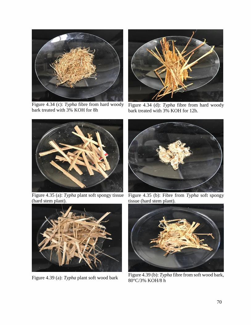
70

Figure 4.34 (c): Typha fibre from hard woody

bark treated with 3% KOH for 8h

Figure 4.34 (d): Typha fibre from hard woody

bark treated with 3% KOH for 12h.

Figure 4.35 (a): Typha plant soft spongy tissue

(hard stem plant). Figure 4.35 (b): Fibre from Typha soft spongy

tissue (hard stem plant).

Figure 4.39 (a): Typha plant soft wood bark

Figure 4.39 (b): Typha fibre from soft wood bark,

80°C/3% KOH/8 h

71

Figure 4.39 (c): Typha fibre from soft wood

bark, 80°C/3% KOH/12 h

Figure 4.40 (a): Typha plant soft spongy tissue

(soft stem plant).

Figure 4.40 (b): Fibre from Typha soft spongy

tissue (soft stem plant), 80°C/3% KOH/8 h

Figure 4.41(a): Typha plant leaves (no stem

plant).

Figure 4.41 (b): Fibre from Typha leaves with

soft spongy tissue (No stem plant), 80°C/3%

KOH/8 h

The characteristics (fibre quality) of these fibres and flakes are summarized in Table 4.9.

For this experiment all treatments no replica was used. It can be seen from this table that fibre is

72

obtained from the whole plant, leaves, and spongy tissue, while no fibre can be obtained from the

hard-woody part. The materials that are obtained from this woody segment of the Typha plants are

100% flake (width: 2mm) for soft stem Typha plant (SS) and hard stem Typha plant (HS) as shown

in [Figure 4.38 (b), (c) and 4.33(b), (c) and (d)], while spongy tissues for (SS) in [Figure 4.40 (b)]

and (HS) [Figure 4.34 (b)] and leaves for both (SS) and (HS) provide 100% fibres as seen in Figure

4.36 (b) and Figure 4.31 (b), however, a few flakes could be found in the fibres obtained from the

whole Typha plant for (SS) [Figure 4.36 (b)] and (HS) [Figure 4.31 (b)].

Further, it appears that the quality of fibres obtained from the spongy tissues is inferior to

those obtained from the Typha leaves, as the leaf fibres are softer and more easily separable than

the fibres from the spongy segment. Fibres from the leaves of the Typha plants are similar to those

from the whole plant as seen in Figures (SS) 4.36 (b) and (HS) 4.31 (b). The woody bark with

spongy tissue is soft but difficult to separate into individual fibres for both (SS) and (HS) plants

[Figures 4.38 (b) and 4.33 (b)]. The same characteristics are shown in the spongy part of the Typha

plant as seen in Figures (SS) 4.40 (b) and (HS) 4.35(b). Fibre yield (%) for the no stem plant was

the highest – 41.33%. The yield (%) of fibre and flake in the soft stem plant was found to be 31.90

(%) and 4.76 (%) respectively, while in the hard stem plant this amount was 26.57% and 11.59%,

respectively. Fibre from leaves gave a comparatively higher yield (%) in (SS), 38.00; whereas, the

(HS) was 29.80; there was no flake (%) for leaves. In (hard wood + spongy tissue), mixed with

fibres and flakes fibre yield (%) was 33.33 and flake (%) was 12.57 for (SS); and for (HS) fibre

yield (%) was 30.66 and flake (%) 21.33. Fibre extracted from spongy tissue segment was fibre

32.66% for (SS) and 21.33 for (HS). There were only flakes (%), but no fibre in the woody bark

section, [1.18 (for 8 hours, SS), 1.64 (for 12 hours, SS); 0.74 (for 6 hours, HS), 1.24 (for 8 hours,

HS), and 1.42 (for 12 hours)].

73

Table 4.12: Fibre yield (%) and visual characteristics of fibres from different plant segment, 3.0% KOH, 80°C after 8 hours.

Typha

plant

segment

Plant

type

Flake

obtained

Fibre

obtained

Yield (%) Figure # dFibre quality (visual)

Plant

weight

(g)

Yield

(%) of

fibre

Yield

(%)

of

flakes

Original

component

After

treatment

Whole

plant

SS Yes Yes 2.10 31.90 4.76

4.36(a) 4.36(b) S, SF

HS Yes Yes 2.07 26.57 11.59 4.31(a) 4.31(b) S, SF

NS No Yes 1.89 41.33 0.00 4.41(a) 4.41(b) S, SF

Leaves

SS No Yes 1.87 38.00 0.00 4.37(a) 4.37(b) S, SF

HS No Yes 1.51 29.80 0.00 4.32(a) 4.32(b) S, SF

Woody

bark +

spongy

tissue

SS Yes

Figure 3.34 (c)

Yes 1.10 33.33 12.57 4.38(a) 4.38(b) S, difficult to separate

HS Yes, 3.29 (c) Yes 1.59 30.66 21.33 4.33(a) 4.33(b) S, difficult to separate

Woody

bark

SS Yes No 1.82 0.00 57.56 4.39(a) 4.39(b) NA

aSS Yes No 2.08 0.00 78.46 4.39(a) 4.39(c) NA bHS Yes No 1.57 NA 36.63 4.34(a) 4.34(b) NA

HS Yes No 2.01 NA 60.78 4.34(a) 4.34(c) NA cHS Yes No 2.03 NA 71.00 4.34(a) 4.34 (d) NA

Spongy

tissue

SS No Yes 1.59 32.66 0.00 4.40(a) 4.40(b) S, difficult to separate

HS No Yes 1.57 21.33 0.00 4.35(a) 4.35(b) S, difficult to separate

NA: Not applicable; SS: Soft stem; HS: hard stem; NS: no stem; a: 12 hours; b: 6 hours; c: 12 hours; d: based on softness (S) and single

(SF) fibre.

74

4.2.1.1 Summary

The most widely used water retting was investigated for fibre extraction from the Typha plant.

Unsuccessful results from water retting showed that this retting method is unsuitable for the Typha

plant, so other extraction methods were employed. Similarly, acid and enzyme retting did not work

for fibre extraction of Typha fibre. Alkali (KOH, LiOH) treatment of less than 2 hours and <3.0%

concentration was not suitable for proper fibre extraction; however, treatment between 2 hours and

8 hours with 3% alkali could produce fibres. The plant physiological investigation found that fibre

yield (%) was influenced by different factors: composition of plants such as flake (%); presence

of an inner woody core section; and plant type: No stems plants provided a higher yield 41.33 %

without 0.0% flakes than hard 26.57 % with flake 11.59% and soft stem 31.90% with 4.76 %

plants. The optimum parameter for obtaining fibres from all three Typha plants was found to be 2

hours / KOH or LiOH at 80°C.

An ideal textile fibre obtain a series of important properties that influence product

performance and helps to choose several fibres for any sort of end uses in textile and apperal

industry. Once fibres are found from chemical retting, it is essential to investigate major

characteristics the textile properties including morphological structure, physical, mechanical, and

thermal aspects. The next chapter will discuss these important textile properties in order to find

out the suitability of Typha fibre for apparel application.

75

CHAPTER 5: TEXTILE CHARACTERISTICS OF TYPHA LATIFOLIA L. FIBRE

For apparel and non-textile applications (medical, geotextiles and bio-composites), fibres

must have both textile properties such as length, diameter, moisture regain, chemical properties

and absorbency and spinning properties such as softness and single fibre entity. In the current

study, selected apparel and spinning properties are measured and discussed. It is worth mentioning

that for this part of the research, the whole Typha plant was used for producing fibres.

5.1 Fibre morphology

Morphological analysis examines the size, shape, and structure of a material and show

relationships between structural properties such as macrostructure, microstructure, submicroscopic

structures and fine structure (Hatch, 1993, p.90).

5.1.1 Macrostructure of Typha fibre

Macrostructure analysis is one of the powerful techniques for studying visible structure

information that helps to characterize the material structure of a fibre. It explores the general nature

of the external surface by the naked eye or by using visible properties and components such as

fibre length and diameter (Agrawal, 1988).

5.1.1.1 Fibre length

An important characteristic of any textile fibre is length, as machine settings, for example,

distance between the drafting rollers during the process of spinning, and depend on fibre length

(Figure 5.1). When the fibre length is longer than the distance between the drafting rollers then

fibre breakage occurs due to the fibre being gripped by both sets of rollers; also, when the fibre

length is shorter than the distance between the drafting rollers then fibre droppings occur (Rohlena,

& Plisek, 1975). Furthermore, fibre length is an important consideration for yarn evenness and

spinning performance in rotor spinning (Kumar, 2015). Fibres are classified into two categories

76

according to length: staple fibres that range in length from ¾ to 18 inches such as Cotton, linum,

cannabis and brassica; and filament (infinite) length fibres such as polyester, nylon and acrylic.

Staple fibres such as Cotton vary in length: Upland Cotton is reported to be between 0.8 to 1.36

inches (Cotton Incorporation, n.d.).

Fibre length influences yarn strength, as longer fibres provide better strength, elongation,

smoothness, and evenness in a spun yarn (Kumar, 2015). A lower amount of twist can be used

when spinning longer fibres, which translates into better efficiency of the spinning frame, as the

speed of the machine is inversely proportional to the amount of twist inserted in a yarn (Rohlena,

& Plisek, 1975). The importance of fibre length and uniformity in fibre length were also discussed

in Section 2.3.1 and 2.3.2 (Chapter 2).

Figure 5.1: A performance of fibre length in spinning processing (A 4 over 3 roller arrangement

drafting systems in a draw frame machine, where 1, 4: back drafting roller, 2, 5: middle drafting

roller, 3, 6: front drafting roller and 7: guide roller) (Hunter, as cited by Khan, 2016).

77

5.1.1.1.1 Relationship between Typha plant length (cut length) and fibre length

Spin limits is the permissible linear density of yarn. The short staple (Cotton) spinning

length varies between 9.5 to 37.5 mm and long staple (wool) spinning length varies usually

between 25.4 to 63.5 mm (Stout, 1960). Man-made fibres are cut 1¼ inches for coarse and medium

yarn count and 1½ inches for fine count, and for blending with Cotton, man-made fibre must cut

to match the length of Cotton. For Typha fibre, length should not be a problem as fibre length

could be controlled up to a certain length by selecting the cut length of the plant. However, two

important characteristics of the fibre should be measured: the relationship between fibre length

and cut length; and length uniformity in a fibre bundle.

Table 5.1 contains the sample ID with treatment time (h) and temperature (°C), original cut

length of Typha plant, average (of 10 fibres) fibre length (mm) with standard deviation. It can be

observed from this table that average fibre length is shorter than the cut length of the Typha plant.

This might be due to the crimp in the fibre. Krowicki et al. (1997) reported that crimp in the fibre

was the major source of error when determining the fibre length.

5.1.1.2 Statistical results

To check whether the plant cut length is same as the fibre length, a statistical analysis was

used that had been suggested by Booth (1968) for smaller fibre sample size (n≤10). The t-statistic

was conducted by comparing the means and standard deviations of the plant cut length and fibre

length. The procedure is given below in which the total mean of seven plant samples and their

standard deviations are used. Using pooled estimate of the sample standard deviation S= 4.5, t-test

was calculated tcal =2.40 > t12 =2.179 (T-table chart), formula given in Appendix XI.

78

Table 5.1: Statistical analysis on the relationship between plants cut length, and fibre length for

different treatments.

Sample ID

(hour / temp °C)

aLength(mm) bLength(mm) cSignificant difference dSignificant difference

S8-K1-MS (2/80) 60.2± 0.00 54.00± 5.30 tcal (3.71)S > t.05 (2.101)S tcal (2.8)S > t.05 (2.101)S

S8-K2-MS (4/80) 60.3± 0.00 54.00± 3.36 tcal (5.9)S > t.05 (2.101)S tcal (4.44)S > t.05 (2.101)S

S8-K3-MS (6/80) 50.0± 0.00 47.00± 6.90 tcal (1.37)n < t.05 (2.101)n tcal (3.03)S > t.05 (2.101)S

S10-L1-MS (2/80) 50.0± 0.00 42.00± 2.83 tcal (8.9)S > t.05 (2.101)S tcal (0.45)n < t.05 (2.101)n



S10-L4-MS (8/80) 50.0± 0.00 39.00±10.10 tcal (3.95S > t.05 (2.101)S tcal (1.02)n < t.05 (2.101)n

Mean 52.974.97S 45.57 6.24S

t-Value, (0.05) 2.45 >2.179 aOriginal plant cut length; bAverage fibre length; nNo significant variation; SSignificant variation; cOriginal cut length vs. Average cut length; dOriginal cut length vs. crimp adjusted length; S:

Sample; K: KOH, L: LiOH; MS: Mixed Stem.

The t-test results are show in Table 5.1, which exhibited that the difference between the

sample means of plant cut length and fibre length is statically significant as tcalc (2.45)> t.05(2.179).

This result rejects the null hypothesis and accept the alternate hypothesis (HA: μ > μ0), the

significant difference between the plants cut length and average fibre length as the original cut

length of Typha plant (M=52.97, SD=4.97) had higher than average length of Typha fibre

(M=45.57, SD =6.24). Moreover, the pair of each fibre sample means to the corresponding mean

of the plant cut length demonstrated a statistically significant difference, as shown in Table 5.1,

except the sample S8-K3-MS, which is not significant.

In Table 5.1, LiOH treated samples (S10-L1-MS, S10-L2-MS, S10-L3-MS and S10-L4-

MS) presented shorter average length 42, 41, 42, and 39 compared to KOH treated average fibre

length S8-K1-MS: 54, S8-K2-MS: 54 and S8-K3-MS: 47, respectively. Further, the visual

observation of the fibre samples revealed that the LiOH treated samples [Figure 5.1 (a)] contain

more short fibres as well as variation in fibre length than the KOH treated fibre [Figure 5.1 (b)].

The researchers found the ratio of 1:1.2 between the measured fibre length and crimp

79

adjusted length for Cotton fibre (Krowicki et al., 1997). The crimp adjusted length of the plants

cut length and average fibre length in Table 5.1 showed that also all KOH treated fibre, S8-K1-

MS (2/80), S8-K2-MS (4/80) and S8-K3-MS (6/80) had a significantly difference in t-test,

whereas, all LiOH treated samples were not significant (Table 5.1). For the current study, statistical

results established that using the ratio of 1:1.2 and considering standard deviation, the fibre length

is almost equal for crimp adjusted four LiOH treated samples length to the cut length of the plant.

As mentioned earlier, for spinning machineries the fibre lengths must be uniform within

1/8 inch (reference). To verify the fibre length variation between two different alkali samples, data

given in Appendix III and shown in Figures 5.1 (a) and 5.1 (b), 15 fibre samples (n = 15) were

randomly chosen from the samples of S8-K4-MS and S10-L4–MS as suggested by ASTM standard

D1440 - 07(2012). Fibre length variation for these two samples is shown in Figure 5.2. The average

and standard deviations were calculated and found to be 40.0 mm 6.0, and 23.0 mm 10.0

respectively for S8-K4-MS and S10-L4-MS.

Figure 5.2 (b): Typha fibre length uniformity treated with KOH (Sample: S8-K4-MS)

(Painted by paint s).

Figure 5.2 (a): Typha fibre length uniformity treated with LiOH (Sample: S10-L4-MS)

(Painted by paint s).

80

Figure 5.3: Fibre length variation between treated Sample S8-K4-MS and S10-L4-MS.

5.1.1.3 Statistical analysis of Typha fibre length: Effect of treatment on fibre length

Using this model a statistical analysis ANOVA was tested to find the effect of

difference in treatment was examined. From the F-test results (F1, 28) = Fcritical (4.20) < Fcal (29.50),

it can be stated that the difference in the fibre lengths between the two treatments (T1 = S8-K4-

MS; T2 = S10-L4-MS) was significant at p = 0.0001 <0.05. Since the difference is significant, the

null hypothesis is rejected. Therefore, the effects of the treatments were shown to be different.

From the F-statistic, it was confirmed that the treatment effects are different. Least squares

difference is used to compare the two treatment means. From the table, the estimate of least squares

means for treatment S8-K4-MS = 4.0267 and the estimate of least square means for treatment S10-

L4-MS = 2.3200. However, to examine whether both treatment effects are necessary for the model,

a t-test was conducted for each estimated treatment effect, where tcritical = 1.701, which is less than

tcal. In both cases, tcal > tcritical and p < 0.05; therefore, the null hypothesis is rejected. In conclusion,

the two alkali-treated samples S8-K4-MS and S10-L4-MS are individually significant and have

different length variations.

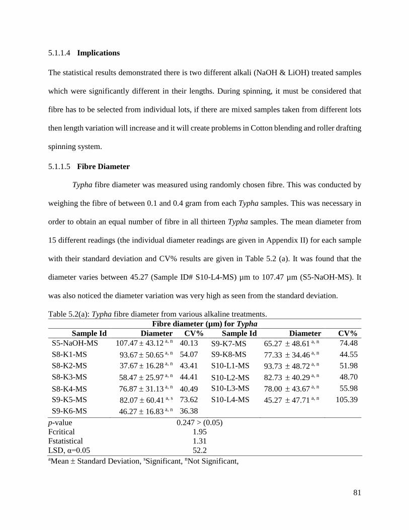
81

5.1.1.4 Implications

The statistical results demonstrated there is two different alkali (NaOH & LiOH) treated samples

which were significantly different in their lengths. During spinning, it must be considered that

fibre has to be selected from individual lots, if there are mixed samples taken from different lots

then length variation will increase and it will create problems in Cotton blending and roller drafting

spinning system.

5.1.1.5 Fibre Diameter

Typha fibre diameter was measured using randomly chosen fibre. This was conducted by

weighing the fibre of between 0.1 and 0.4 gram from each Typha samples. This was necessary in

order to obtain an equal number of fibre in all thirteen Typha samples. The mean diameter from

15 different readings (the individual diameter readings are given in Appendix II) for each sample

with their standard deviation and CV% results are given in Table 5.2 (a). It was found that the

diameter varies between 45.27 (Sample ID# S10-L4-MS) µm to 107.47 µm (S5-NaOH-MS). It

was also noticed the diameter variation was very high as seen from the standard deviation.

Table 5.2(a): Typha fibre diameter from various alkaline treatments.

Fibre diameter (µm) for Typha

Sample Id Diameter CV% Sample Id Diameter CV%

S5-NaOH-MS 107.47 ± 43.12 a, n 40.13 S9-K7-MS 65.27 48.61 a, n 74.48

S8-K1-MS 93.67 50.65 a, n 54.07 S9-K8-MS 77.33 34.46 a, n 44.55

S8-K2-MS 37.67 ± 16.28 a, n 43.41 S10-L1-MS 93.73 48.72 a, n 51.98

S8-K3-MS 58.47 25.97 a, n 44.41 S10-L2-MS 82.73 40.29 a, n 48.70

S8-K4-MS 76.87 31.13 a, n 40.49 S10-L3-MS 78.00 43.67 a, n 55.98

S9-K5-MS 82.07 60.41 a, s 73.62 S10-L4-MS 45.27 47.71 a, n 105.39

S9-K6-MS 46.27 16.83 a, n 36.38

p-value 0.247 > (0.05)

Fcritical 1.95

Fstatistical 1.31

LSD, α=0.05 52.2 aMean Standard Deviation, sSignificant, nNot Significant,

82

Table 5.2(a) showed that Typha fibre samples obtained higher diameter CV% value, when

it was taken by random selection method. The alkali differences and due to the presence of group

fibre in a single fibre. The resultant CV% was higher which indicates larger the diameter variation.

With such larger diameter variation, it would be difficult to make yarn with uniform diameter.

A statistical experiment was performed using a single Factor ANOVA to determine

whether there was a difference in diameter between the Typha samples. The difference in diameter

is not found to be significant as p = 0.247>0.05 (Table 5.2 (a)). However, the Fisher LSD test

exhibits a significant difference between the means of S5-NaOH-MS and S8-K2-MS (69.8>52.2),

S5-NaOH-MS and S9-K6-MS (61.2>52.2), S5-NaOH-MS and S10L4-MS, (62.2>52.2), S8-K1-

MS and S8-K2-MS, (56>52.2), S9K7-MS and S10-L1-MS, (93.73>52.2), S8-K2-MS and S10-L1-

MS, (56.06>52.2), respectively (Table 5.2(b)). No other comparisons were found to be significant,

which was due to the larger variation among the diameters.

Table 5.2(b): Fisher’s LSD test to compare the difference

Between pairs of means for diameter of the thirteen Typha fibre.

Group 1 (Y1) Group 2 (Y2) ∣Y1- Y2∣

S5-NaOH-MSS S8-K2-MSS 69.8(>52.2)S

S5-NaOH-MSS S9-K6-MSS 61.2(>52.2)S

S5-NaOH-MSS S10-L4-MSS 62.2(>52.2) S

S9-K7-MSS S10-L1-MSS 93.7(>52.2)S

S8-K1-MSS S8-K2-MSS 56.0(>52.2)S

S8-K2-MSS S10-L1-MSS 56.1(>52.2)S sSignificant, LSD (α=0.05) =52.2

The diameter data obtained from random sampling of Typha fibre showed the larger

diameter than the Cotton and wool fibres as the diameter of these two fibres varies between 10 to

25 µm (Hatch, 2006). Therefore, no comparison was made between Typha fibres with Cotton and

wool. However, during diameter measurements, it was noticed that the Typha fibre was not a single

fibre as the fibre comprised of multiple single fibre. To compare the diameter of Typha with Cotton

and wool, single Typha fibres were collected from biological Typha sample S8-K3-MS.

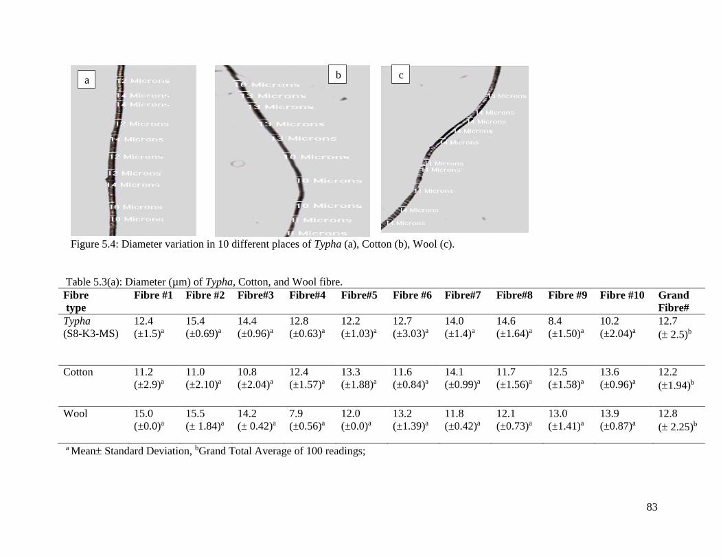
83

Figure 5.4: Diameter variation in 10 different places of Typha (a), Cotton (b), Wool (c).

Table 5.3(a): Diameter (µm) of Typha, Cotton, and Wool fibre.

Fibre

type

Fibre #1

Fibre #2 Fibre#3

Fibre#4

Fibre#5

Fibre #6

Fibre#7

Fibre#8

Fibre #9

Fibre #10

Grand

Fibre#

Typha

(S8-K3-MS)

12.4

(±1.5)a

15.4

(±0.69)a

14.4

(±0.96)a

12.8

(±0.63)a

12.2

(±1.03)a

12.7

(±3.03)a

14.0

(±1.4)a

14.6

(±1.64)a

8.4

(±1.50)a

10.2

(±2.04)a

12.7

( 2.5)b

Cotton 11.2

(±2.9)a

11.0

(±2.10)a

10.8

(±2.04)a

12.4

(±1.57)a

13.3

(±1.88)a

11.6

(±0.84)a

14.1

(±0.99)a

11.7

(±1.56)a

12.5

(±1.58)a

13.6

(±0.96)a

12.2

(1.94)b

Wool 15.0

(±0.0)a

15.5

(± 1.84)a

14.2

(± 0.42)a

7.9

(±0.56)a

12.0

(±0.0)a

13.2

(±1.39)a

11.8

(±0.42)a

12.1

(±0.73)a

13.0

(±1.41)a

13.9

(±0.87)a

12.8

( 2.25)b

a Mean Standard Deviation, bGrand Total Average of 100 readings;

a b

c

84

5.1.1.6 Statistical analysis

A statistical test was carried to measure the significant difference of the fibre diameter

between Typha and Cotton and Typha & Wool fibres using SAS II.

Table 5.4(a): Statistical summary of Typha and Cotton fibre diameter.

Fibre Mean

(µm)

Std Dev Std Err Minimum

(µm)

Maximum

(µm)

Variance

Typha (S8-K3-MS)

12.71 2.54 0.26 7.00 18.00 6.43

Cotton 12.22 1.94 0.19 8.00 15.00 3.75

Fcal 1.72

Fcritical 1.39

Levene’s F test (p-value) 0.0078 (< 0.05)

t-test (p-value) 0.1263 (> 0.05)

N = 100 samples each of Typha and Cotton fibres.

Table 5.4(a) summarizes Typha and Cotton diameters, where the maximum value for

Typha is 18 µm, and for Cotton is 15 µm and the minimum value for Typha is 7 µm, and for Cotton

is 8 µm. The mean value of Typha and Cotton is almost similar: 12.7 µm and 12.2 µm.

Equality of variances (Table 5.5) between Typha versus Cotton shows that p= 0.0078 <

0.05 and Fcritical (1.39) < Fcal (1.72). So the null hypothesis is rejected. Therefore, the variances for

Typha and Cotton are not equal.

Since the variance analysis determines that the variances between Typha and Cotton were

not equal, therefore, the Satterthwaite method was used to conduct the t-test for unequal variance.

The t-test formulas are given in (Appendix VIII). Null hypothesis: d1 = d2. The diameters of Typha

and Cotton are equal. Alternative hypothesis: d1 ≠ d2. The diameters of the Typha and Cotton are

not equal. The t-test results revealed that p= 0.1263 > .05, so, the null hypothesis has been shown

in Table 5.4(a). Therefore, the diameter of Cotton and Typha were deemed to be equal.

85

Table 5.4(b): Statistical summary of Typha and Wool fibre diameter.

Fibre Mean

(µm)

Std Dev Std Err Minimum

(µm)

Maximum

(µm)

Variance

Typha (S8-K3-MS) 12.71 2.54 0.26 7.00 18.00 6.43

Wool 12.86 2.25 0.22 7.00 18.00 5.05

Fcal 1.27

Fcritical 1.39

Levene’s F test (p-value) 0.2314 (> 0.05)

t-test (p-value) 0.6585 (> 0.05)

N = 100 samples each of Typha and Wool fibres.

Table 5.4(b) shows that the maximum and minimum value for Typha and Wool are both

the same value. The mean value of Typha and Wool is almost the same: 12.7 µm and 12.8 µm.

First, the homogeneity of the variances was examined in order to perform the t-test correctly. From

the equality of variances between Typha and Wool it was found that Fcritical (1.39) > Fcal (1.27), p =

0.2314 > .05, so we accept the null hypothesis. Therefore, the variances are equal. The t-test was

performed using the pooled method considering the variances are equal. Null hypothesis: d1 = d3.

The diameters of Typha and wool are equal. Alternative hypothesis: d1 ≠ d3. The diameters of the

Typha and Wool are not equal. The t-test revealed that p= 0.6585 > .05. So, we accept the null

hypothesis. Therefore, the diameter of Typha and wool were deemed to be statistically equal.

It can be concluded that there is no significant difference in the diameters of Typha, Cotton

and wool fibres. Therefore, Typha fibre could be a replacement for wool or Cotton in Cotton

spinning system. It should be mentioned that in case of multiple t-test comparisons, type I () error

rate is inflated. However, the comparison error rate (c) was .05, and the experimental error rate

(E) was .00975.

5.1.1.7 Summary

It can be concluded that from the macrostructure analysis, Typha fibre is suitable for Cotton

spinning systems, though fibre length uniformity of Typha depends on the type of alkaline

chemical treatment. The hypothesis of t-test established that, Typha fibre is similar to wool fibre

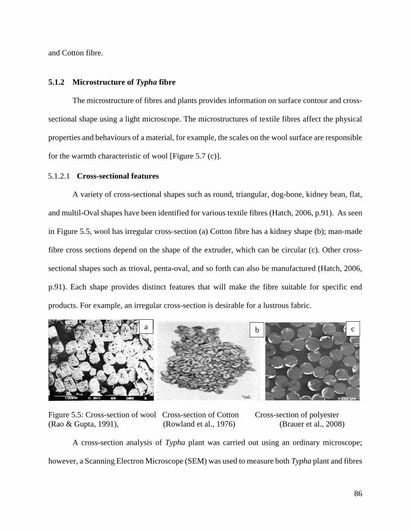
86

and Cotton fibre.

5.1.2 Microstructure of Typha fibre

The microstructure of fibres and plants provides information on surface contour and cross-

sectional shape using a light microscope. The microstructures of textile fibres affect the physical

properties and behaviours of a material, for example, the scales on the wool surface are responsible

for the warmth characteristic of wool [Figure 5.7 (c)].

5.1.2.1 Cross-sectional features

A variety of cross-sectional shapes such as round, triangular, dog-bone, kidney bean, flat,

and multil-Oval shapes have been identified for various textile fibres (Hatch, 2006, p.91). As seen

in Figure 5.5, wool has irregular cross-section (a) Cotton fibre has a kidney shape (b); man-made

fibre cross sections depend on the shape of the extruder, which can be circular (c). Other cross-

sectional shapes such as trioval, penta-oval, and so forth can also be manufactured (Hatch, 2006,

p.91). Each shape provides distinct features that will make the fibre suitable for specific end

products. For example, an irregular cross-section is desirable for a lustrous fabric.

Figure 5.5: Cross-section of wool Cross-section of Cotton Cross-section of polyester

(Rao & Gupta, 1991), (Rowland et al., 1976) (Brauer et al., 2008)

A cross-section analysis of Typha plant was carried out using an ordinary microscope;

however, a Scanning Electron Microscope (SEM) was used to measure both Typha plant and fibres

a b c

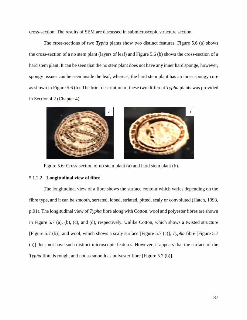
87

cross-section. The results of SEM are discussed in submicroscopic structure section.

The cross-sections of two Typha plants show two distinct features. Figure 5.6 (a) shows

the cross-section of a no stem plant (layers of leaf) and Figure 5.6 (b) shows the cross-section of a

hard stem plant. It can be seen that the no stem plant does not have any inner hard sponge, however,

spongy tissues can be seen inside the leaf; whereas, the hard stem plant has an inner spongy core

as shown in Figure 5.6 (b). The brief description of these two different Typha plants was provided

in Section 4.2 (Chapter 4).

Figure 5.6: Cross-section of no stem plant (a) and hard stem plant (b).

5.1.2.2 Longitudinal view of fibre

The longitudinal view of a fibre shows the surface contour which varies depending on the

fibre type, and it can be smooth, serrated, lobed, striated, pitted, scaly or convoluted (Hatch, 1993,

p.91). The longitudinal view of Typha fibre along with Cotton, wool and polyester fibres are shown

in Figure 5.7 (a), (b), (c), and (d), respectively. Unlike Cotton, which shows a twisted structure

[Figure 5.7 (b)], and wool, which shows a scaly surface [Figure 5.7 (c)], Typha fibre [Figure 5.7

(a)] does not have such distinct microscopic features. However, it appears that the surface of the

Typha fibre is rough, and not as smooth as polyester fibre [Figure 5.7 (b)].

a b

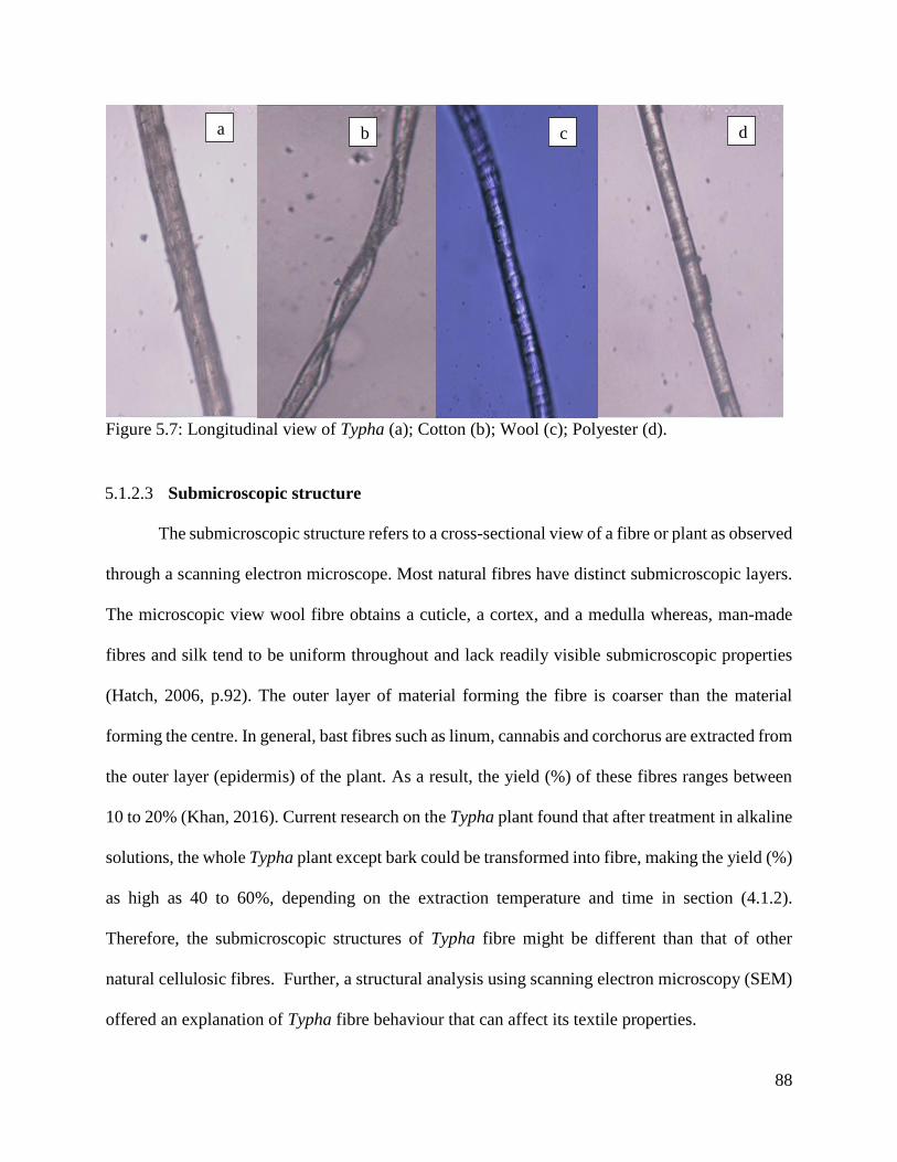
88

Figure 5.7: Longitudinal view of Typha (a); Cotton (b); Wool (c); Polyester (d).

5.1.2.3 Submicroscopic structure

The submicroscopic structure refers to a cross-sectional view of a fibre or plant as observed

through a scanning electron microscope. Most natural fibres have distinct submicroscopic layers.

The microscopic view wool fibre obtains a cuticle, a cortex, and a medulla whereas, man-made

fibres and silk tend to be uniform throughout and lack readily visible submicroscopic properties

(Hatch, 2006, p.92). The outer layer of material forming the fibre is coarser than the material

forming the centre. In general, bast fibres such as linum, cannabis and corchorus are extracted from

the outer layer (epidermis) of the plant. As a result, the yield (%) of these fibres ranges between

10 to 20% (Khan, 2016). Current research on the Typha plant found that after treatment in alkaline

solutions, the whole Typha plant except bark could be transformed into fibre, making the yield (%)

as high as 40 to 60%, depending on the extraction temperature and time in section (4.1.2).

Therefore, the submicroscopic structures of Typha fibre might be different than that of other

natural cellulosic fibres. Further, a structural analysis using scanning electron microscopy (SEM)

offered an explanation of Typha fibre behaviour that can affect its textile properties.

a b c d

89

The cross-section of a Typha leaf is interconnected by a number of ribs. Microscopic

examination shows a ‘crenelated’ (rectangular indentation) structure: small ridges corresponding

to the fibres can clearly be seen and felt with a thumbnail (Figure 5.12). The ribs and outer surface

of the leaf act mechanically and build a protective shield to bending deflections. The (SEM) reveals

that the Typha fibres lie inside the epidermal layer of the leaf.

The cross-section of the Typha plant is divided into two distinct layers: the outer layer

(epidermis, cross-sectional area 38.5 mm2) and the inner layer (probable fibre layer, area 20.1

mm2) (Figure 5.8). The ratio of fibre to plant area is 52.0%, which is within the range of fibre

yield (%). The general structure of the cross section of a Typha fibre consists of numerous small

elliptical, radially-shaped cells, each about 4.5 – 6.0 µm, (Figure 5.9) and about 0.70 µm apart in

a group cell of 740 µm (Figure 5.10). Each cell has a lumen (≈1.03 µm) (as shown in Figure 5.5)

in the middle that indicates the maturity of the fibre cell (Hatch, 2006) and defines fibre strength

and fineness. The fibre cells are not attached to each other, as there is a ‘canal’ between the cells.

The structure of the cells provides the potential for multiple excellent textile properties (dyeing

absorbency, diameter, thermal properties, fibre flexibility and easy fibre separation).

The crenelated structure may positively contribute to good dye absorbency and thermal

insulation; the fibres are very easy to separate, making them suitable for spun yarn conversion; the

diameter of the Typha fibre is comparable to Cotton and wool; the fibre cell has a lumen, and the

cells are separated by canal, a feature that might have significant implications in biomedical

applications for trapping antibiotics and other chemicals. The yield (%) is about 54%, which is

close to the ratio of total plant area to inner (probable fibre) area. From the morphological studies,

it is concluded that the Typha fibre could be used for both textile and biomedical applications.

90

Figure 24

Figure 5.8: Cross-section area of Typha plant Figure 5.9: Individual cell size and distance

with two distinct layers of Typha Fibre

Figure 5.10: A group of Typha fibre Figure 5.11: Polygonal ultimate cells with

diameter lumen size

Figure 5.12: Small ridges ‘crenelated ‘structure of

Typha leaf (rectangular indentation) structure.

91

Table 5.5: Summary of Typha microscopic study.

Microscopic Characteristic Properties Figure no.

Two distinct layers

38.5 mm2 (outer layer area)

and 20.1 mm2 (inner layer area)

5.8

Individual cell size and distance of Typha fibre

4.5 – 6.0 µm/cell 5.9

Typha fibre diameter in group 30.0 µm 5.10

Cell lumen size 1.03 µm 5.11

‘Crenelated’ structure of Typha leaf (rectangular

indentation)

Small ridges 5.12

5.2 Typha fibre chemical composition analysis by Fourier Transform Infrared

Spectroscopy (FTIR)

The primary polymer components of the cell wall, cellulose, hemicellulose, and lignin, are

comprised in natural plants (Zheng et al., 2017). Cellulose, the main element of polysaccharides,

which are principle components in natural plant fibres, acts as the supporting material in the cell

wall (Zheng et al., 2017). The cellulose molecules are bonded in a microfibril structure in which

there is extensive hydrogen bonding between cellulose chains, producing a strong crystalline

structure (Thomas et al., 2013). FTIR is one of the most important analytical and advanced tools

used to obtain information on the super-molecular structure and chemical compositions of Typha

fibre. FTIR spectra were taken between 500-4000 cm-1 wave numbers for Typha no stem plant

(leaf + sponge), and Typha fibres obtained from alkaline treatments. The FTIR spectrum of Typha

(leaf + sponge), fibre was compared with Cotton, Typha leaf and cannabis fibre from the literature.

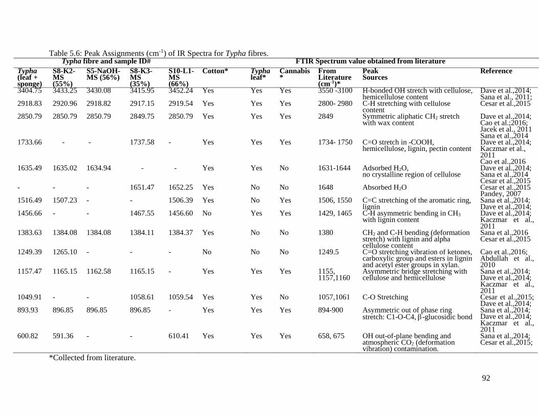
92

Table 5.6: Peak Assignments (cm-1) of IR Spectra for Typha fibres. Typha fibre and sample ID# FTIR Spectrum value obtained from literature

Typha (leaf + sponge)

S8-K2-MS (55%)

S5-NaOH-MS (56%)

S8-K3-MS (35%)

S10-L1-MS (66%)

Cotton* Typha leaf*

Cannabis*

From Literature (cm-1)*

Peak Sources

Reference

3404.75 3433.25 3430.08 3415.95 3452.24 Yes Yes Yes 3550 -3100 H-bonded OH stretch with cellulose, hemicellulose content

Dave et al.,2014; Sana et al., 2011; Cesar et al.,2015 2918.83 2920.96 2918.82 2917.15 2919.54 Yes Yes Yes 2800- 2980 C-H stretching with cellulose

content 2850.79 2850.79 2850.79 2849.75 2850.79 Yes Yes Yes 2849 Symmetric aliphatic CH2 stretch

with wax content Dave et al.,2014; Cao et al.;2016; Jacek et al., 2011 Sana et al.,2014

1733.66 - - 1737.58 - Yes Yes Yes 1734- 1750 C=O stretch in -COOH, hemicellulose, lignin, pectin content

Dave et al.,2014; Kaczmar et al., 2011 Cao et al.,2016

1635.49 1635.02 1634.94 - - Yes Yes No 1631-1644 Adsorbed H2O, no crystalline region of cellulose

Dave et al.,2014; Sana et al.,2014 Cesar et al.,2015

- - - 1651.47 1652.25 Yes No No 1648 Absorbed H2O Cesar et al.,2015 Pandey, 2007

1516.49 1507.23 - - 1506.39 Yes No Yes 1506, 1550 C=C stretching of the aromatic ring, lignin

Sana et al.,2014; Dave et al.,2014;

1456.66 - - 1467.55 1456.60 No Yes Yes 1429, 1465 C-H asymmetric bending in CH3 with lignin content

Dave et al.,2014; Kaczmar et al., 2011

1383.63 1384.08 1384.08 1384.11 1384.37 Yes No No 1380 CH2 and C-H bending (deformation stretch) with lignin and alpha cellulose content

Sana et al.,2016 Cesar et al.,2015

1249.39 1265.10 - - - No No No 1249.5 C=O stretching vibration of ketones, carboxylic group and esters in lignin and acetyl ester groups in xylan.

Cao et al.,2016; Abdullah et al., 2010

1157.47 1165.15 1162.58 1165.15 - Yes Yes Yes 1155, 1157,1160

Asymmetric bridge stretching with cellulose and hemicellulose

Sana et al.,2014; Dave et al.,2014; Kaczmar et al., 2011

1049.91 - - 1058.61 1059.54 Yes Yes No 1057,1061 C-O Stretching Cesar et al.,2015; Dave et al.,2014;

893.93 896.85 896.85 896.85 - Yes Yes Yes 894-900 Asymmetric out of phase ring stretch: C1-O-C4, -glucosidic bond

Sana et al.,2014; Dave et al.,2014; Kaczmar et al., 2011

600.82 591.36 - - 610.41 Yes Yes Yes 658, 675 OH out-of-plane bending and atmospheric CO2 (deformation vibration) contamination.

Sana et al.,2014; Cesar et al.,2015;

*Collected from literature.

93

Table 5.6 shows the peak assignments of FTIR spectra using KBr pellet method obtained

from Typha (leaf + sponge), and fibre (S8- K2-MS, S5-NaOH-MS, S8-K3-MS and S10-L1-MS) are

given in Appendix IV (Figures 5.13 and 5.14(a) to 5.14(e)). IR spectra for Cotton, Typha, and Cannabis

fibres collected from literature are compared with Typha (leaf + sponge) and fibres.

The most important component of cellulosic materials is cellulose, a fibre forming group.

As with Cotton and other cellulosic materials, this group is dominant in Typha fibres. The

cellulosic groups in Typha (leaf + sponge) and fibres can be found at wavenumber of 3433.25 cm−1

(peak range: 3550 -3100) that corresponds to H-bonded OH stretch with cellulose, and

hemicellulose content. This band can be found in Typha (leaf+sponge), Typha fibres (S8-K2-MS,

S5-NaOH-MS, S8-K3-MS and S10-L1-MS), Cotton (Dave et al., 2014), Typha (Cesar et al. 2015)

and Cannabis fibre (Kaczmar et al., 2011). The band at 2918.83 cm−1 in the Typha (leaf+sponge)

and fibres falls within the frequency range of 2800 – 2980 cm−1 which is C-H stretching with

cellulose content. Such groups can also be found in Cotton (Dave et al. 2014), Typha (Cesar et al.,

2015) and Cannabis fibres (Kaczmar et al., 2011). The cellulose group (asymmetric bridge

stretching) is found in the frequency range of 1155 cm-1 to 1165 cm-1 for Typha (leaf + sponge),

Typha fibres except S10-L1-MS samples as well as Cotton, Typha leaf and Cannabis fibres (Table

5.12). Another component of cellulosic materials is wax which can represent up to 5.0% and is

removed before wet processing treatment by scouring (McCall & Jurgens, 1951). The wax group

attributed to symmetric aliphatic CH2 stretch in Typha materials [Figures 5.14 (a) – 5.14(f)], Cotton

(Dave et al., 2014), Typha (Cao et al., 2016) and Cannabis (Kaczmar et al., 2011) can be found at

2850 cm-1. The hemicellulose, lignin, pectin content can be found at the wave number 1733.66

cm−1 due to the C=O stretch in –COOH. These peaks can be found only in Typha (leaf + sponge)

and one Typha fibre sample (S8-K3-MS), Cotton, Typha and Cannabis fibre. The absence of this

group in samples S8-K2-MS, S5-NaOH-MS and S10-L1-MS may be because of the removal of

94

hemicellulose, lignin, and pectin during alkaline treatment. The peaks due to the absorbed water,

in the range of 1631-1644 cm-1 and 1648 cm-1, can be seen for both Typha plants and Cotton.

However, only Typha fibre samples of S8-K2-MS and S5-NaOH-MS exhibit a water group at 1635

cm-1; S8-K3-MS and S10-L1-MS samples showed a water group in the range of 1651 cm-1 to 1652

cm-1. No such peaks can be found for Cannabis, and only in the range of 1631-1644 cm-1 for Typha.

The lignin groups are observed at multiple peaks. These peaks, at wave lengths 1516 cm-1,

1456 cm-1, 1383 cm-1 and 1249 cm-1 for Typha plants, belong to an aromatic ring in lignin, C-H

asymmetric bending in CH3 with lignin, CH2 and C-H bending (deformation stretch) with lignin,

and C=O stretching vibration of ketones, carboxylic group and esters in lignin as well as acetyl

ester groups in xylan, respectively. For Typha fibres, only 1507 cm-1, 1384 cm-1 and 1265 cm-1 can

be found for S8-K2-MS sample; 1384 cm-1 for S5-NaOH-MS; 1467 cm-1 and 1384 cm-1 for S8-

K3-MS; and 1506 cm-1, 1456 cm-1 and 1384 cm-1 for S10-L1-MS samples. Such presence and

absence of lignin groups in Typha fibres cannot be explained without further research. However,

this behaviour is also found for Cotton (Dave et al., 2014), Typha leaf (Cesar at al., 2015) and

Cannabis fibre (Kaczmar et al., 2011) as recorded in Table 5.12. One of the major bonds is the -

glucosidic bond which connects repeating units of cellubiose in the cellulosic materials. This bond

can be found at the frequency range of 894 cm-1 to 900 cm-1 in all samples except S10-L1-MS. It

was noticed that fibres in this sample were broken into smaller lengths during extraction and the

absence of -glucosidic bond may be the reason for the shorter fibre length.

Finally, the IR spectra of untreated Typha (leaf+sponge) and Typha fibres show similar

characteristic features related to cellulose, lignin, hemicellulose, and wax components that also

can be found in Cotton, Typha leaf and Cannabis fibres. It was noticed that Typha leaf does not

exist CH2 and C-H bending (deformation stretch) with lignin and alpha cellulose and C=O

95

stretching vibration of ketones, carboxylic group and esters in lignin and acetyl ester groups in

xylan content whereas Typha (leaf+sponge) and fibre sample S8-K2-MS have that contents may

be the presents of spongy materials.

5.3 Moisture Regain (%) of Typha plants and fibre

Moisture is an important term in textiles that relates to wearer comfort, shrinkage, rate of

drying and static electricity (Taylor, 1972). Moisture regain (%) is calculated according to the

formula given in Section 3.3.4. The moisture regain (%) of Typha plants and fibre obtained from

various treatments and conditions (relative humidity and temperature) is given in Tables 5.7(a) For

comparison, wool fibre (raw), whose moisture regain has already been established, is also

determined. The use of wool fibre helped to determine the accuracy of the moisture regain

measurement process as literature values for wool are available.

Table 5.7(a): Moisture regain (%) of Typha plants at various humidity and temperatures.

Sample type Conditioning atmosphere

(RH% and temp °C)

Conditioning

duration

(hour)

Drying time (hour)

temperature (°C)

Moisture

regain (%)

Virgin Typha plant 50%, 20°Ca 12 4/105 9.4

Virgin Typha plant 50%, 20°C a 12 8/105 12.7

Virgin Typha plant 70%, 16°C c 12 8/105 9.8 1Virgin Typha plant 61%, 24.9°C b 72 10/105 10.6 2Virgin Typha plant 59%, 25°C b 72 10/105 9.6

Wool fibre(raw) 70%, 16°C b 12 8/105 9.6 1Wool fibre (raw) 61%, 24.9°C b 72 10/105 11.1 2Wool fibre (raw) 59%, 25°C b 72 10/105 8.8

Wool (raw) 65%, 21°C a *≥8 Until constant

weight/105

11.0

1 sample was conditioned from atmospheric condition; 2 sample was conditioned from dry state. aconditioning room, bhumidity chamber, coutside weather.*Literature value of Wool (Booth, 1968)

The moisture regain (%) for Typha plant ranges from 9.4 to 12.7 (Table 5.7(a)). For the

same relative humidity (RH% = 50), the increase in drying time from four hours to eight hours

enhances the moisture regain (%) by about 35% (Table 5.7(a), Rows 1 & 2). To determine the

96

hysteresis of Typha plants, samples were conditioned from atmospheric condition and dry state.

The moisture regain (%) was 10.6 and 9.6 for Typha samples conditioned from atmospheric and

dry states respectively (Table 5.7(a), Rows 4 & 5) and the difference in moisture regain was found

to be 1.0%.

A similar experiment was conducted for wool fibre and the hysteresis was found to be

2.3%. The hysteresis value for wool fibre varies depending on the wool fibre type (woolen,

worsted), yarn type and other factors. However, a more reasonable value is 2.1% as reported by

(Cookson and Slota, 1993). The experimental moisture regain (%) obtained from the current study

for wool fibre is similar to the published value (Booth, 1968). The measured moisture regain (%)

following chemical treatment for Typha fibre, (considering relative humidity) is shown in Table

5.7(b).

Table 5.7(b) shows the average moisture regain at 50% relative humidity and 20°C

temperature, standard deviations and CV% of various Typha samples. The average moisture regain

(%) for the Typha fibres varies between 3.69 (S8-K3) and 10.9 (S8K2). The moisture regain for

most of the Typha fibres is lower than the Typha plant (9.57%) except S8-K2 sample (10.90%). A

t-test experiment was conducted (formula given in Appendix XI) to investigate significant

difference between Typha, Wool and Cotton shown in Appendix VI. It was found Typha and wool

fibres has significant difference tcal (2.461) > tstatistical (2.179), however, Typha and Cotton fibre

were not statistically significant, tcal (0.759) < tstatistical (2.179) in Table 5.7(b).

The statistical analysis of ANOVA test found no significant difference among these

samples (Table 5.7(b)). However, the Fisher’s LSD test was conducted and found significant

variation between Typha plant and S8K3-MS (5.87>4.58), S8K3-MS and S8K4-MS (5.34>4.58),

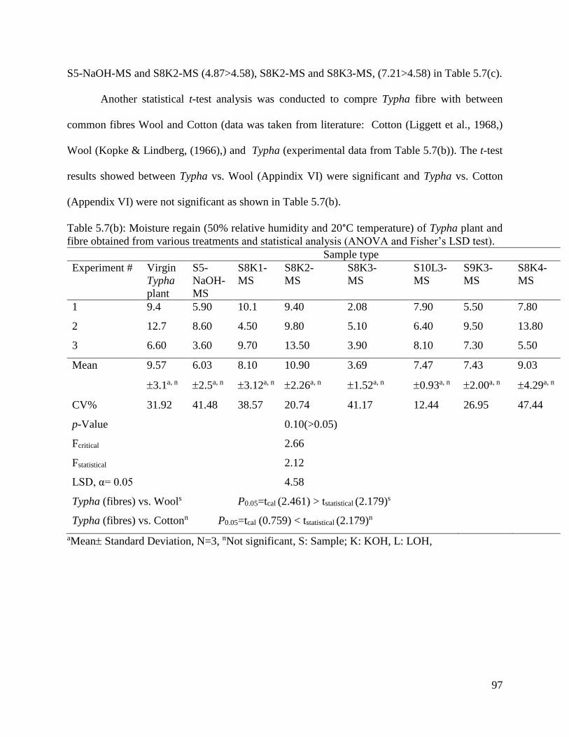
97

S5-NaOH-MS and S8K2-MS (4.87>4.58), S8K2-MS and S8K3-MS, (7.21>4.58) in Table 5.7(c).

Another statistical t-test analysis was conducted to compre Typha fibre with between

common fibres Wool and Cotton (data was taken from literature: Cotton (Liggett et al., 1968,)

Wool (Kopke & Lindberg, (1966),) and Typha (experimental data from Table 5.7(b)). The t-test

results showed between Typha vs. Wool (Appindix VI) were significant and Typha vs. Cotton

(Appendix VI) were not significant as shown in Table 5.7(b).

Table 5.7(b): Moisture regain (50% relative humidity and 20°C temperature) of Typha plant and

fibre obtained from various treatments and statistical analysis (ANOVA and Fisher’s LSD test).

Sample type

Experiment # Virgin

Typha

plant

S5-

NaOH-

MS

S8K1-

MS

S8K2-

MS

S8K3-

MS

S10L3-

MS

S9K3-

MS

S8K4-

MS

1 9.4 5.90 10.1 9.40 2.08 7.90 5.50 7.80

2 12.7 8.60 4.50 9.80 5.10 6.40 9.50 13.80

3 6.60 3.60 9.70 13.50 3.90 8.10 7.30 5.50

Mean 9.57

3.1a, n

6.03

2.5a, n

8.10

3.12a, n

10.90

2.26a, n

3.69

1.52a, n

7.47

0.93a, n

7.43

2.00a, n

9.03

4.29a, n

CV% 31.92 41.48 38.57 20.74 41.17 12.44 26.95 47.44

p-Value 0.10(>0.05)

Fcritical 2.66

Fstatistical 2.12

LSD, α= 0.05 4.58

Typha (fibres) vs. Wools P0.05=tcal (2.461) > tstatistical (2.179)s

Typha (fibres) vs. Cottonn P0.05=tcal (0.759) < tstatistical (2.179)n

aMean Standard Deviation, N=3, nNot significant, S: Sample; K: KOH, L: LOH,

98

Table 5.7(c): The comparison of moisture regain (%) between pair of means for Typha plant and

fibres by Fisher’s LSD test.

Group 1 (Y1) Group 2 (Y2) ∣Y1- Y2∣ Group 1 (Y1) Group 1 (Y1) ∣Y1- Y2∣ Virgin typha plantn S5-NaOH-MSn n 3.53(<4.58)n S5-NaOH-MS n S8K1-MS n 2.07(<4.58)n

Virgin typha plantn S8K1-MS n 1.47(<4.58)n S5-NaOH-MS S S8K2-MS S 4.87(>4.58)S

Virgin typha plantn S8K2-MS n 1.33(<4.58)n S5-NaOH-MS n S8K3-MS n 2.34(<4.58)n

Virgin typha plantS S8K3-MSS 5.87(>4.58)S S5-NaOH-MS n S10L3-MS n 1.43(<4.58)n

Virgin typha plantn S10L3-MS n 2.10(<4.58)n S5-NaOH-MS n S9K3-MS n 1.40(<4.58)n

Virgin typha plantn S9K3-MS n 2.13(<4.58)n S5-NaOH-MS n S8K4-MS n 3.00(<4.58)n

Virgin typha plantn S8K4-MS n 0.53(<4.58)n S8K2-MS S S8K3-MS S 7.21(>4.58)S

S8K1-MSn S8K2-MS n 2.80(<4.58)n S8K2-MS n S10L3-MS n 3.43(<4.58)n

S8K1-MS n S8K3-MS n 4.41(<4.58)n S8K2-MS n S9K3-MS n 3.47(<4.58)n

S8K1-MS n S10L3-MS n 0.63(<4.58)n S8K2-MS n S8K4-MS n 1.87(<4.58)n

S8K1-MS n S9K3-MS n 0.67(<4.58)n S8K3-MS n S10L3-MS n 3.77(<4.58)n

S8K1-MS n S8K4-MS n 0.93(<4.58)n S10L3-MS n S9K3-MS n 0.03(<4.58)n

S8K3-MS n S9K3-MS n 3.74(<4.58n) S10L3-MS n S8K4-MS n 1.57(<4.58)n

S8K3 -MS S S8K4-MS S 5.34(>4.58)S S9K3-MS n S8K4-MS n 1.60(<4.58)n nNo significant variation, SSignificant variation, S: Sample; K: KOH, L: LOH,

Summary

The properties of textile are strongly affected by moisture regain. In addition, moisture

regain will help to determine dimension, mechanical strength and elastic recovery and rigidity.

The Typha plant and fibre absorbed moisture in different humidity atmosphere and provided

various moisture regains, Typha plant was found 9.57% (average) and Typha fibre was found

10.90% (average). Statistical analysis said that moisture regain of Typha is similar with Cotton but

different with Wool.

5.4 Thermal Properties

In textiles, when fibres are exposed to a heat source, some ignite and burn while others are

non-combustible. Fibres that ignite but do not continue to burn, whether or not the ignition source

is removed, are called flame resistant. Fibres that do not shrink or burn readily when heat is applied

have a property known as thermal stability. The flammability of a textile may be used as a basis

of selection for its use in different products. A thermal-resistant fabric has the ability to act as

thermal insulator, (in garments) preventing a dangerous elevation of skin temperature. A fabric

99

also needs to be heat-resistant and heat durable to maintain properties during and following

exposure to high temperature.

Depending on the end-use, a manufacturer can make thermal fabric suitable for firefighters,

foundry workers, welders, race-car drivers and astronauts, who are all exposed to intense radiant

heat, flame, and/or molten metal splashes in the work environment. Burning of small quantities of

textile fibres may be used as a means of distinguishing one fibre group from another. Precise

identification of individual fibres by burning is not usually possible; however, burning behaviour

can readily establish the general fibre group to which the fibre belongs. Cellulosic fibres exhibit

flammability characteristics much like those of paper; protein fibres burn in a manner similar to

hair and some man-made fibres melt when they burn. Some fibres produce an odour when they

burn, and the remaining ash residue can also assist to identify the fibre.

5.4.1 Burning behaviour of Typha fibre

The Burn-test response was carried out to observe how Typha fibres respond to flame. Two

widely used fibres, Cotton and polyester, were used to compare the burning behaviour of Typha

fibre. The burning behaviour of these three fibres is shown in Table 5.8.

Three different steps were evaluated during this test: when fibres approach a flame, when

they are in the flame and when they are removed from the flame. When Cotton and Typha fibres

approach flame, they do not shrink or fuse but produce white smoke and have a smell of paper or

wood burning; whereas, polyester shrinks, fuses, produces black smoke and has a chemical and

sweet smell. In the flame, Cotton and Typha rapidly burn, but polyester burns slowly. Polyester

melts and does not continue to burn in the flame, while Cotton and Typha continues burning with

an afterglow, but do not appear to melt in the flame. This result is given Table 5.8.

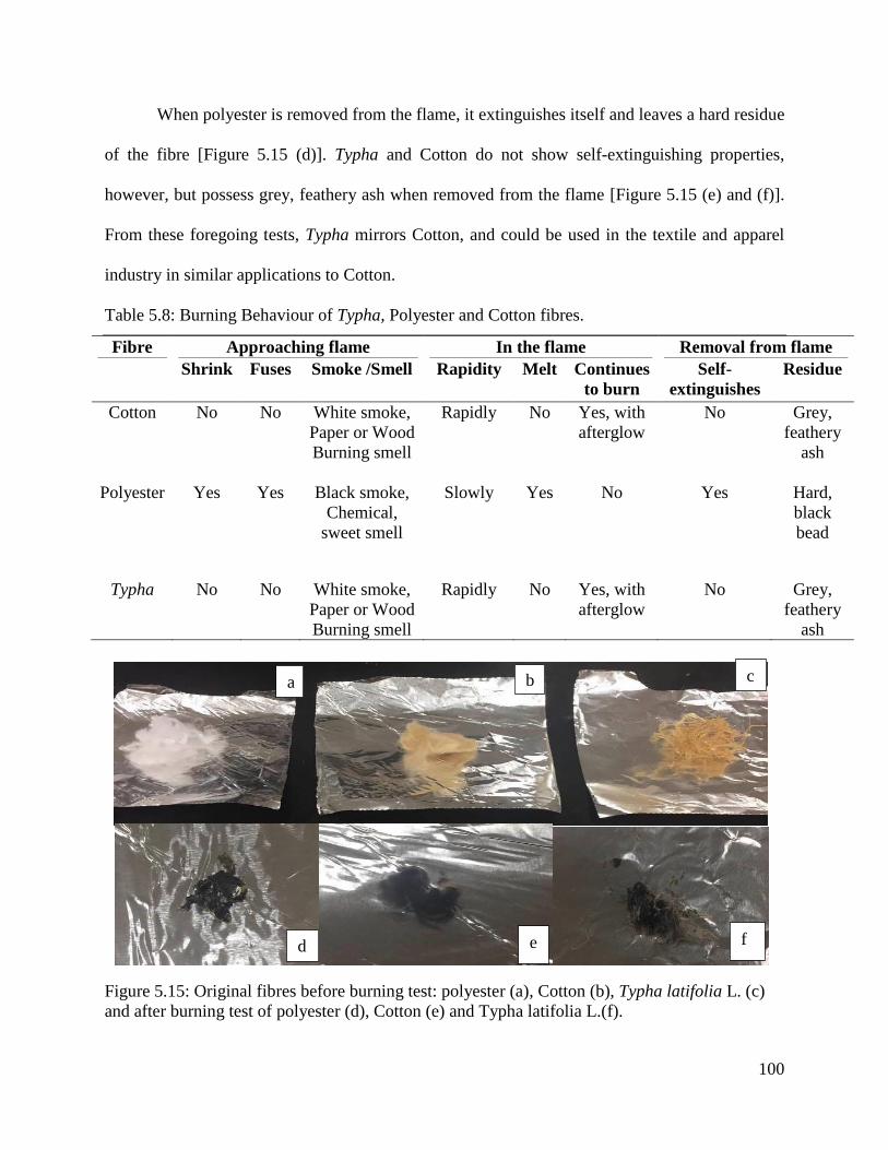
100

When polyester is removed from the flame, it extinguishes itself and leaves a hard residue

of the fibre [Figure 5.15 (d)]. Typha and Cotton do not show self-extinguishing properties,

however, but possess grey, feathery ash when removed from the flame [Figure 5.15 (e) and (f)].

From these foregoing tests, Typha mirrors Cotton, and could be used in the textile and apparel

industry in similar applications to Cotton.

Table 5.8: Burning Behaviour of Typha, Polyester and Cotton fibres.

Fibre Approaching flame In the flame Removal from flame

Shrink Fuses Smoke /Smell Rapidity Melt Continues

to burn

Self-

extinguishes

Residue

Cotton No No White smoke,

Paper or Wood

Burning smell

Rapidly No Yes, with

afterglow

No Grey,

feathery

ash

Polyester Yes Yes Black smoke,

Chemical,

sweet smell

Slowly Yes No Yes Hard,

black

bead

Typha No No White smoke,

Paper or Wood

Burning smell

Rapidly No Yes, with

afterglow

No Grey,

feathery

ash

Figure 5.15: Original fibres before burning test: polyester (a), Cotton (b), Typha latifolia L. (c)

and after burning test of polyester (d), Cotton (e) and Typha latifolia L.(f).

a b c

d e f

101

5.4.2 Evaluation of Typha fibre thermal properties

Fibre decomposition temperature is measured to determine the ability of a fibre to

withstand dyeing or other high temperature manufacturing and laundering procedures. The thermal

behaviour of Typha plant, Typha (S10L3-MS) fibre and Cotton fibre are presented in Table 5.9. In

order to obtain the thermal decomposition point, the machine was set to run up to 300°C with no

intermediate holding temperature or holding time. The decomposition point was recorded when

the fibre turned dark brown or yellow colour as shown in Figures 5.16, 5.17, and 5.18 for Typha

plant, Typha (S10L3-MS) fibre and Cotton fibre, respectively. The virgin Typha plant samples

[Figures 5.16 (a)] that turn dark brown at 234.9°C [Figure 5.16 (b)] and chemically treated Typha

(S10L3-MS) fibre [Figure 5.17 (a)] which turn dark brown at 268.7°C in Figure 5.17 (b) and

likewise Cotton fibre Figure 5.18 (a) decomposed at 248.3°C shown in Figures 5.18 (b). The result

indicates that the Typha (S10L3-MS) fibres are thermally stable up to 268.7°C, while the Cotton

decomposed at 248.3°C. The lower decomposition temperature for Typha plant than the Typha

(S10L3-MS) fibre may be due to the presence of lower amounts of non-cellulosic materials in the

Typha fibre.

Table 5.9: Thermal properties of Typha plant, Typha fibre and Cotton fibre

Material type Decomposition

temperature

(°C)

Comments

Figure #

Virgin sample Decomposed

sample

Typha latifolia L. Plant 234.9 Fibres turn dark brown 5.16(a) 5.16(b)

Typha fibre (S10L3-MS) 268.7 Fibres turn dark brown 5.17(a) 5.17(b)

Cotton fibre 248.3 Fibres turn dark brown 5.18(a) 5.18(b)

102

Figure 5.16(a): Virgin Typha plant. Figure 5.16(b): Decomposed Typha plant.

Figure 5.17(a): Virgin Typha fibre. Figure 5.17(b): Decomposed Typha fibre.

Figure 5.18(a): Virgin Cotton fibre. Figure 5.18(b): Decomposed Cotton fibre.

In textile applications, thermal stability is considered as an important parameter. For

household textiles and many industrial applications, fibres are exposed to high temperature for

long periods of time, such as curtains, rugs, tarpaulins and other products. To determine the thermal

behaviour at different temperatures and holding times, seven individual samples of Typha (S10L3-

MS) and Cotton fibres were prepared from a fibre bundle. For this test, the holding time used to

evaluate changes of sample colour performance by colour software (Colour Hexa) at specific

temperature and after a specific time. Typha (S10L3-MS) and Cotton sample images were

imported to graphics software called paint application; using this application all images were

103

cropped measured by scale (gridline). Each image was cropped 4x4 (gridlines) and created image

palette. These images are given in Appendix VI.

Then these image colour palettes exported into image software image colour picker (from

https://www.colorcodepicker.com). The software gave HEX color code of the pixel value (for

example TTF1 HEX value is #baad90) given in details correspondent pictures and HEX value are

given in Appendix VIII. The original pictures Figure 5.19 (a) – 5.32(a) for 10 minutes holding

time and Figure 3.19(b) – Figure 5.32(b) for 20 minutes holding time which are taken from Linkam

are given in Appendix VIII. To convert HEX pixel value to Hunter-Lab L* value, by software

called ColorHexa (from https://www.colorhexa.com). The L* value of colour descriptions was

provided in Table 5.10(a). It is worth mentioning here that the lower the L* value, the darker the

sample.

It can be seen from this Table 5.10(a) that with the increasing temperature the L value has

been decreased for both Cotton and Typha fibres at both 10 and 20 minutes holding times. The

changes in colour with the heating temperature and holding time are shown in Figures 5.19 (b) –

5.32 (b). These figures are given in Appendix VIII.

It is seen that for Typha fibre, increase of temperature from 120°C to 300°C with 30°C

interval, the L value was decreased to 6.75 (Sample code: TTF7) from 65.07 (Sample code: TTF1)

and 7.55 (Sample code: TTF7) from 45.99 (Sample code: TTF1) for 10 and 20 minutes holding

time, respectively. Similar trend was observed for Cotton fibre 11.82 (Sample code: TGF7) from

60.70 (Sample code: TGF1) and 8.3 (Sample code: TGF7) from 47.03 (Sample code: TGF1). A

graphpical presentation given in Figure 5.33.

104

5.4.2.1. Summary

Longer stability in heat is a sign of a good quality fibre that is suitable for textile

applications. It was observed that Typha (S10L3-MS) fibres have heat resistance capacity,

exceeding that of Cotton when heated directly from 0°C to 300°C without any holding time (Table

5.9). However, it appears that Cotton is more heat resistant than Typha fibre when both fibres are

heated using holding times (Table 5.10(a)).

105

Table 5.10(a): Thermal properties of Typha and Cotton fibre with different temperatures range.

Sample

type

Temperature

Range (°C)

Colour changing effect

Holding Time: 10(min) Holding Time: 20 (min)

HEX

value

L* Value Colour

description

Figure HEX

value

L* Value Colour

description

Figure

TTF1 120 #baad90 65.07 GO 5.19 (a) #a2854d 49.99 DMO 5.19 (b)

TTF2 150 #897e61 45.94 DDO 5.20 (a) #8f703e 42.16 DMO 5.20 (b)

TTF3 180 #795c2c 34.50 DMO 5.21 (a) #574126 24.39 VDDO 5.21 (b)

TTF4 210 #8c6d3b 41.02 DMO 5.22 (a) #523c25 22.71 VDDO 5.22 (b)

TTF5 240 #331f12 13.14 VDO 5.23 (a) #4f3a24 21.95 VDDO 5.23 (b)

TTF6 270 #2e1a0a 11.58 VDBO 5.24 (a) #2b1b12 11.58 VDBO 5.24 (b)

TTF7 300 #130d0d 6.75 VDBR 5.25 (a) #151011 7.55 VDBR 5.25 (b)

TGF1 120 #a4a49c 60.70 DGY 5.26 (a) #81827d 47.03 DGY 5.26 (b)

TGF2 150 #a4a49b 60.67 DGY 5.27 (a) #82847b 47.62 DGY 5.27 (b)

TGF3 180 #9c9c8e 57.27 DGY 5.28 (a) #83847e 47.79 DGY 5.28 (b)

TGF4 210 #6c5d47 33.87 VDGO 5.29 (a) #7c6a4c 38.89 MDDO 5.29 (b)

TGF5 240 #675a44 32.58 VDGO 5.30 (a) #5e4229 25.37 VDDO 5.30 (b)

TGF6 270 #3c2c1d 16.89 VDDO 5.31 (a) #36281e 15.48 VDDO 5.31 (b)

TGF7 300 #291d13 11.82 VDBO 5.32 (a) #1e1310 8.83 VDBR 5.32 (b)

TTF: Temperatue of Typha Fibre; TCF: Temperature of Cotton Fibre; Figure 5.18 (a) – 5.31(a) and Figure 3.18(b) – Figure 5.31(b)

shown in Appendix V; *GO: Grayish orange; *DDO: Dark desaturated orange; *DMO: Dark moderate orange; *VDO: Very dark

orange; *VDBO: Very dark (mostly black) orange; *VDBR: Very dark (mostly black) red; *DGY: Dark grayish yellow; *VDGO:

Very dark grayish orange*VDDO: Very dark desaturated orange; MDDO: Mostly desaturated dark orange.

106

Figure 5.33: Changes in L* Value with temperature for Cotton and Typha fibres.

5.5 Dyeing of Typha fibres with reactive dye

Cellulosic fibres are dyed predominantly with reactive dyes in the presence of salt and in

alkaline conditions. The dye fixation efficiency of reactive dyes on cellulosic fibres varies between

50-90% (Cai et al., 1999). As shown through the IR spectra (Section 5.2), Typha. fibres consist

mainly of chemical groups related to cellulose.

Typha fibres from different extraction treatments were dyed, and then washed with HCl

50% (v/v) to determine the dye retention by the samples (shown in Figures 5.34 – 5.40). It can be

seen that the fibres retain the reactive colour. For comparison, Cotton fibre was also dyed (Figure

5.34) with the same dye and dye bath parameters.

One of the objectives of dyeing is to produce a uniform colouration throughout a material.

Visual observation showed no colour variation within the sample from various extracted fibre

0

10

20

30

40

50

60

70

1 2 0 1 5 0 1 8 0 2 1 0 2 4 0 2 7 0 3 0 0

L* V

ALU

E(%

)

TEMPERATURE(℃)

COLOUR CHANGING EFFECT

L value_Cotton_10min L value_Typha_10min

L value_Cotton_20min L value_Typha_20min

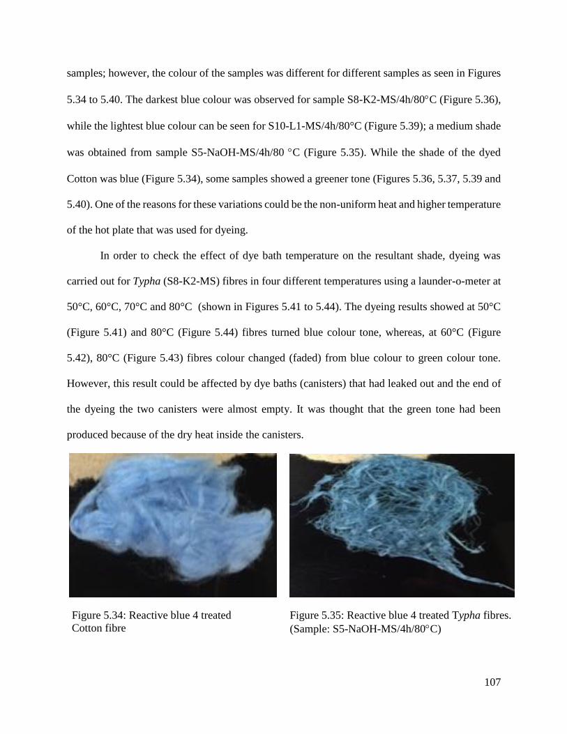
107

samples; however, the colour of the samples was different for different samples as seen in Figures

5.34 to 5.40. The darkest blue colour was observed for sample S8-K2-MS/4h/80C (Figure 5.36),

while the lightest blue colour can be seen for S10-L1-MS/4h/80°C (Figure 5.39); a medium shade

was obtained from sample S5-NaOH-MS/4h/80 C (Figure 5.35). While the shade of the dyed

Cotton was blue (Figure 5.34), some samples showed a greener tone (Figures 5.36, 5.37, 5.39 and

5.40). One of the reasons for these variations could be the non-uniform heat and higher temperature

of the hot plate that was used for dyeing.

In order to check the effect of dye bath temperature on the resultant shade, dyeing was

carried out for Typha (S8-K2-MS) fibres in four different temperatures using a launder-o-meter at

50°C, 60°C, 70°C and 80°C (shown in Figures 5.41 to 5.44). The dyeing results showed at 50°C

(Figure 5.41) and 80°C (Figure 5.44) fibres turned blue colour tone, whereas, at 60°C (Figure

5.42), 80°C (Figure 5.43) fibres colour changed (faded) from blue colour to green colour tone.

However, this result could be affected by dye baths (canisters) that had leaked out and the end of

the dyeing the two canisters were almost empty. It was thought that the green tone had been

produced because of the dry heat inside the canisters.

Figure 5.34: Reactive blue 4 treated

Cotton fibre

Figure 5.35: Reactive blue 4 treated Typha fibres.

(Sample: S5-NaOH-MS/4h/80C)

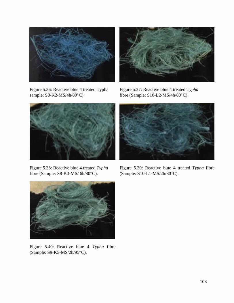
108

Figure 5.36: Reactive blue 4 treated Typha

sample: S8-K2-MS/4h/80C).


fibre (Sample: S10-L2-MS/4h/80C).


fibre (Sample: S8-K3-MS/ 6h/80C).

Figure 5.39: Reactive blue 4 treated Typha fibre

(Sample: S10-L1-MS/2h/80C).

Figure 5.40: Reactive blue 4 Typha fibre

(Sample: S9-K5-MS/2h/95C).

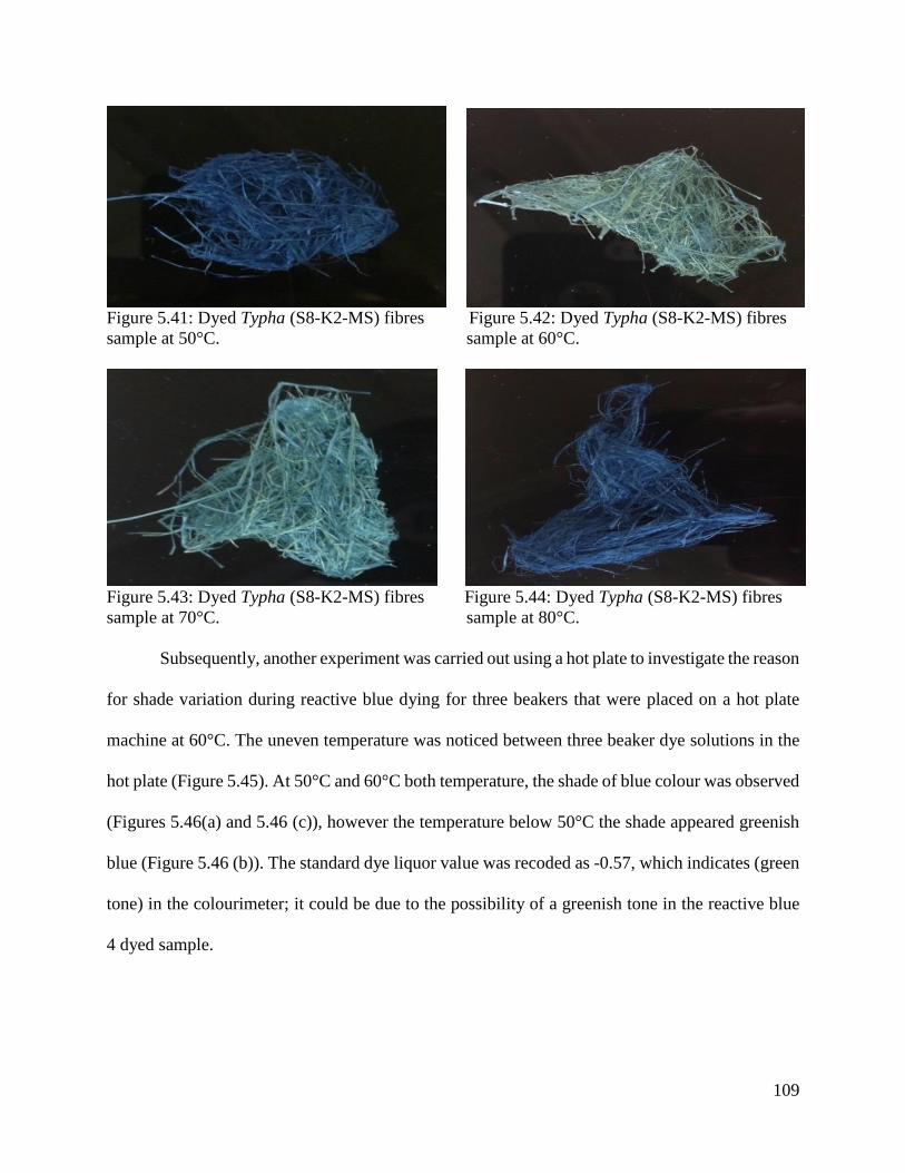
109

Figure 5.41: Dyed Typha (S8-K2-MS) fibres Figure 5.42: Dyed Typha (S8-K2-MS) fibres

sample at 50°C. sample at 60°C.

Figure 5.43: Dyed Typha (S8-K2-MS) fibres Figure 5.44: Dyed Typha (S8-K2-MS) fibres

sample at 70°C. sample at 80°C.

Subsequently, another experiment was carried out using a hot plate to investigate the reason

for shade variation during reactive blue dying for three beakers that were placed on a hot plate

machine at 60°C. The uneven temperature was noticed between three beaker dye solutions in the

hot plate (Figure 5.45). At 50°C and 60°C both temperature, the shade of blue colour was observed

(Figures 5.46(a) and 5.46 (c)), however the temperature below 50°C the shade appeared greenish

blue (Figure 5.46 (b)). The standard dye liquor value was recoded as -0.57, which indicates (green

tone) in the colourimeter; it could be due to the possibility of a greenish tone in the reactive blue

4 dyed sample.

110

Figure 5.45: Temperatures variation on dye liquor solution in different place of the hot plate.

Figure 5.46: Shade variation of dyed Typha sample in hot plate test (a: at 60 C) (b: less than 50

C) and (c: 50 C temperature).

5.5.1 Evaluation of colour fastness of dyed Typha fibres

The colourfastness of dyed textile materials is required to ensure that there is no colour

transfer during washing, colour removal by light/heat/perspiration/ironing/pressing, or colour

rubbing off by crocking/abrasion during end uses or on exposure to such conditions. For the current

research, only colour fastness to hot pressing was conducted. In the hot-pressing colour fastness

method, the dyed samples are placed between two hot plates and pressure is applied as outlined in

Section 3.3.10 (Chapter 3). In this colourfastness test, three methods were adopted: dry, damp and

wet pressing according to AATCC standard test method: 133-2009 (AATCC, 1985).

Before the colour fastness test, ten (10) evaluators were trained to evaluate the colour

difference and staining. No colour changes or staining was obtained for the dry test and therefore,

no data is provided. The colour changes and staining data from the ten evaluators for damp and

a b c

111

wet tests are provided in Tables 5.11 (a) and 5.12 (a). The colour change of the dyed Typha fibre

to the wet undyed Cotton fabric was evaluated because water often is sprayed onto fabric during

ironing/pressing. For ease of identification, a two-character sample ID is given with the existing

sample ID for each data point which is provided in the parenthesis (Table 5.11(a)). For example,

existing sample ID S10-L2-MS is given 1.A as identifier and the wet undyed Cotton fabric at 110

°C/15 second is identified as 1.B [Table 5.11(a)].

In damp pressing, the lowest rating obtained was between 3.18 (Sample: 3.A, data: 3.C)

among other samples at 110°C. All dry undyed Cotton samples stained less than the wet undyed

Cotton samples. At 110°C, the rating of the difference of staining between dry undyed Cotton

fabrics and wet undyed Cotton fabric was between 0.6 (Sample: 3.A) and 0.10 (Sample: 2.A). At

150°C, the largest difference, 0.35, obtained for sample 1.A and the smallest difference, 0.05,

found for sample 7.A. The difference was almost similar at 200 °C: 0.3 for sample 6.A and 0.04

for sample 5.A. The rating of colour change for the damp test was lower than the staining rating

for all the samples in all three temperatures. For example, for sample S10-L2-MS (1.A), the

staining rating is 4.7 in wet undyed Cotton fabric; whereas, the colour change was 4.05 [Table

5.11(a)]. Further, it was noticed that the change in colour for four samples (1.G, 2.G, 6.G and 7.G)

was higher (lower rating) when temperature was raised from 110°C to 200°C. For the other three

samples (3.G, 4.G and 5.G), the rating was higher. It is worth mentioning here that Cotton fibre

and Typha fibre behave almost the same: the colour change rating was found 4.4 at 110 °C/15

second (7.C); 4.49 at 150°C/15 second (7.E) and 4.19 at 200°C/15 second (7.G).

For the wet pressing test, the staining rating of wet undyed Cotton fabric was lower than

the dry undyed Cotton fabric for all samples and all temperatures as seen Table 5.12 (a). Further,

112

the wet staining rating is lower at 150 °C and 200 °C for all Typha fibres than the wet staining at

110 °C, and the changes in colour are higher at 150 °C and 200 °C than 110 °C.

Two-way ANOVA was conducted for both damp pressing and wet pressing samples in

order to identify the difference of colour fastness and staining among the fibre samples. The

dependent variables for this analysis were two staining conditions (Dry undyed Cotton fabric for

staining and wet undyed Cotton fabric for staining) and one colour change condition (Rating for

colour change). The comparison was made for all three treatment temperatures: 110°C/15 sec,

150°C/15 sec and 200°C/15 sec and interactions among treatment conditions (dependent variables)

and temperatures.

113

Table 5.11(a): Colour fastness rating in hot press method (damp pressing) for Typha fibres.

Damp pressing temperature (°C) / time (second)

110 /15 150/15 200/15

Sample ID Rating for

staining

Rating for

CC

Rating for

staining

Rating for CC Rating for staining Rating for CC

Dry

undyed

Cotton

fabric

Wet

undyed

Cotton

fabric

Dry

undyed

Cotton

fabric

Wet

undyed

Cotton

fabric

Dry

undyed

Cotton

fabric

Wet

undyed

Cotton

fabric

S10-L2-MS

(1.A)

4.95

0.15

4.70.25

(1.B)

4.050.43

(1.C)

4.95

0.15

4.60.35

(1.D)

3.940.60

(1.E)

4.95

0.15

4.850.33

(1.F)

4.180.45 (1.G)

S10-L1-MS

(2.A)

5.0

0.0

4.90.21

(2.B)

4.350.41

(2.C)

4.95

0.15

4.850.3

3 (2.D)

3.741.17

(2.E)

4.9

0.21

4.70.42

(2.F)

3.750.40 (2.G)

S8-K3-MS

(3.A)

5.0

0.0

4.40.31

(3.B)

3.180.60

(3.C)

4.95

0.15

4.60.40

(3.D)

4.080.42

(3.E)

5.0

0.0

4.950.15

(3.F)

3.950.68 (3.G)

S9-K5-MS

(4.A)

4.85

0.24

4.40.31

(4.B)

3.540.80

(4.C)

4.95

0.15

4.70.34

(4.D)

4.250.26

(4.E)

4.95

0.15

4.7 0.34

(4.F)

3.670.95 (4.G)

S8-K2-MS

(5.A)

5.0

0.0

4.60.31

(5.B)

3.440.80

(5.C)

4.95

0.15

4.80.25

(5.D)

4.750.26

(5.E)

4.94

0.15

4.90.21

(5.F)

4.130.69 (5.G)

S5-NaOH-MS

(6.A)

4.95

0.15

4.70.34

(6.B)

4.190.37

(6.C)

4.95

0.15

4.70.34

(6.D)

3.890.62

(6.E)

5.0

0

4.70.26

(6.F)

3.750.84 (6.G)

Cotton (7.A) 5.0

0.0

4.80.34

(7.B)

4.40.39 (7.C) 4.9

0.21

4.850.3

4 (7.D)

4.490.60

(7.E)

4.95

0.15

4.90.21

(7.F)

4.190.92 (7.G)

114

Table 5.12(a): Colour fastness rating in hot press method (wet pressing) for Typha fibres.

Wet pressing temperature (°C) / time (seconds)

110 /15 150/15 200/15

Sample ID Rating for staining Rating

for CC

Rating for staining Rating

for CC

Rating for staining Rating for

CC Dry

undyed

Cotton

fabric

Wet

undyed

Cotton

fabric

Dry

undyed

Cotton

fabric

Wet

undyed

Cotton

fabric

Dry

undyed

Cotton

fabric

Wet

undyed

Cotton

fabric

S10-L2-MS (1.A) 4.750.26 4.020.4

8 (1.H)

3.641.1

4 (1.I)

4.50.23 4.030.4

7 (1.J)

4.010.9

5 (1.K)

4.650.3

4

3.850.89

(1.L)

3.590.74

(1.M)

S10-L1-MS (2.A) 4.50.23 3.750.4

0 (2.H)

4.50.62

(2.I)

4.080.7

1

3.040.9

9 (2.J)

4.330.6

2 (2.K)

4.390.4

8

3.870.75

(2.L)

3.970.96

(2.M)

S8-K3-MS (3.A) 50 4.290.3

7 (3.H)

4.440.5

1 (3.I)

4.450.3

7

3.250.8

7 (3.J)

3.460.9

3 (3.K)

4.390.4

8

3.780.72

(3.L)

3.940.65

(3.M)

S9-K5-MS (4.A) 4.950.15 4.140.3

6 (4.H)

4.150.6

7 (4.I)

4.90.21 4.280.9

5 (4.J)

4.280.5

7 (4.K)

4.60.31 3.930.61

(4.L)

3.720.56

(4.M)

S8-K2-MS (5.A) 4.490.43 3.810.3

8 (5.H)

4.50.40

(5.I)

3.880.6

3

3.080.8

3 (5.J)

3.50.92

(5.K)

4.50.23 3.510.60

(5.L)

4.090.70

(5.M)

S5-NaOH-MS (6.A) 4.80.26 3.910.7

0 (6.H)

3.680.8

6 (6.I)

4.590.5

4

3.40.80

(6.J)

3.950.8

1 (6.K)

4.230.5

2

3.340.81

(6.L)

3.760.72

(6.M)

Cotton (7.A) 50 3.870.5

4 (7.H)

4.650.4

1 (7.I)

4.80.25 3.620.6

0 (7.J)

4.140.6

0 (7.K)

4.750.3

5

4.240.44

(7.L)

3.770.83

(7.M)

115

Table 5.11(b): Two-way ANOVA results tests on the effect of temperature and treatments on

colour fastness for damp pressing.

Dependent Variable

Independent Variable (Temperature) Independent variable (Treatment)

Temperature Mean

Std.

Error Treatment Mean

Std.

Error

Dry undyed Cotton

fabric

110°C 4.784 .046 S8-K2 4.290 0.070

150°C 4.464 .045 S8-K3 4.630 0.070

200°C 4.501 .046 S10-L1 4.323 0.070

S10-L2 4.633 0.070

S9-K5 4.817 0.070

S5-NaOH 4.540 0.070

Cotton 4.850 0.070

Wet undyed Cotton

fabric

110°C 3.967 .081 S8-K2 3.467 0.123

150°C 3.545 .080 S8-K3 3.803 0.124

200°C 3.789 .081 S10-L1 3.553 0.123

S10-L2 3.967 0.123

S9-K5 4.117 0.123

S5-NaOH 3.550 0.123

Cotton 3.910 0.123

Rating for staining 110°C 4.230 .090 S8-K2 4.030 0.137

150°C 3.960 .089 S8-K3 3.979 0.137

200°C 3.834 .090 S10-L1 4.267 0.137

S10-L2 3.747 0.137

S9-K5 4.050 0.137

S5-NaOH 3.797 0.137

Cotton 4.187 0.137

Treatments

Dry undyed Cotton fabric for stainingn Fcalculated (0.634)n P=(0.703 > α =0.05)n

Wet undyed Cotton fabric for stainings Fcalculated (2.388)s P=(0.030 < α =0.05)s

Rating for colour change s Fcalculated (3.088) s P=(0.007 < α =0.05)s

Temperature

Dry undyed Cotton fabric for stainingn Fcalculated(0.367) n P=(0.693 > α =0.05)n

Wet undyed Cotton fabric for stainings Fcalculated (5.184) s P=(0.006 < α =0.05)s


Treatment *

Temperature

Dry undyed Cotton fabric for stainingn Fcalculated(0.776) n P=(0.675> α =0.05)n

Wet undyed Cotton fabric for stainings Fcalculated (1.585)s P=(0.099< α =0.05)s

Rating for colour changes Fcalculated (3.237)s P=(0.0005< α =0.05)s

s: Significant, n: Not Significant,

Table 5.12(b): Two-way ANOVA results tests on the effect of temperature and treatments on

colour fastness for wet pressing.

116

Dependent Variable

Independent Variable (Temperature) Independent variable (Treatment)

Temperature Mean

Std.

Error Treatment Mean

Std.

Error

Dry undyed Cotton

fabric

110°C 4.784 .046 S8-K2 4.290 0.070

150°C 4.464 .045 S8-K3 4.630 0.070

200°C 4.501 .046 S10-L1 4.323 0.070

S10-L2 4.633 0.070

S9K5 4.817 0.070

S5-NaOH 4.540 0.070

Cotton 4.850 0.070

Wet undyed Cotton

fabric

110°C 3.967 .081 S8-K2 3.467 0.123

150°C 3.545 .080 S8-K3 3.803 0.124

200°C 3.789 .081 S10-L1 3.553 0.123

S10-L2 3.967 0.123

S9K5 4.117 0.123

S5-NaOH 3.550 0.123

Cotton 3.910 0.123

Rating for staining 110°C 4.230 .090 S8-K2 4.030 0.137

150°C 3.960 .089 S8-K3 3.979 0.137

200°C 3.834 .090 S10-L1 4.267 0.137

S10-L2 3.747 0.137

S9K5 4.050 0.137

S5-NaOH 3.797 0.137

Cotton 4.187 0.137

Treatments

Dry undyed Cotton fabric for stainings Fcalculated (9.780)s P=(0.0005 > α =0.05)s

Wet undyed Cotton fabric for stainings Fcalculated (4.030)s P=(0.001 < α =0.05)s

Rating for colour changes Fcalculated (1.915)s P=(0.080 > α =0.05)s

Temperature

Dry undyed Cotton fabric for stainings Fcalculated(14.47)s P=(0.0005 > α =0.05)s

Wet undyed Cotton fabric for stainings Fcalculated (6.899) s P=(0.001 < α =0.05)s


Treatment *

Temperature

Dry undyed Cotton fabric for stainings Fcalculated(2.460) s P=(0.05 < α =0.05)s

Wet undyed Cotton fabric for stainingn Fcalculated (1.689)n P=(0.072 > α =0.05)n

Rating for colour changes Fcalculated (1.895)s P=(0.037< α =0.05)s

s: Significant, n: Not Significant,

117

Table 5.13: Results of Post Hoc tests for the effect of hot pressing to colour fastness.

Two-way multivariate ANOVA was conducted for each dependent variable. The results showed.

in Table (5.11(b)), that treatment and temperature during damp testing, for wet undyed Cotton

fabric staining and colour change ratings are significantly different with P=0.030<α =0.05 and

p=0.007< α =0.05 for treatments and P=0.030<α =0.05 and P=0.007<α=0.05), respectively. For

dry undyed Cotton fabric for staining, the treatment and temperature effects are not significant

(treatment: p=0.703>α =0.05; temperature: P=0.693>α =0.05). Similar results were obtained for

interaction between treatment*temperature (Table 5.12(b)).

Post-hoc comparisons using the Tukey HSD test, given in Table 5.13, indicated that there

was a significant pairwise difference of mean temperature for damp hot pressing wet undyed

Cotton fabric (staining) for Cotton and S9K5 (p < .039), while for colour change the significant

pairwise differences were obtained for S8-K3 and Cotton (p < .005), and S9K5 and Cotton (p <

.027),

During wet pressing test, no significant difference was obtained for colour change. However, for

staining, it was noticed that dependant variable dry undyed Cotton fabric for staining was shown

Damp hot pressing Wet hot pressing

Post Hoc multi comparison

Sig. D Post Hoc multi

comparison

Sig. D

Dry undyed

Cotton fabric

(staining)

N/A N/A Dry

undyed

Cotton

fabric

for stating

S8-K2 vs. S8-K3

S8-K2 vs. S10-L2

S8-K2- vs. S9-K5

S8-K2 vs. Cotton

S8-K3 vs. S8-K2

S10-L1 vs. S10-L2

(p= .02)

(p= .011)

(p= .000)

(p= .000)

(p= .021)

(p= .032)

Wet undyed

Cotton fabric

(staining)

S9K5 vs. Cotton (p=.039)

Wet

undyed

Cotton

fabric

S8-K2 vs. S9K5

S10L1 vs. S9K5

S9K5 vs. S5-NaOH

(p=.005)

(p=.024)

(p=.023)

Rating for

colour change

S8-K3 vs. Cotton

S9K5 vs. Cotton

(p=.005)

(p=.027)

Rating for

colour

change

N/A N/A

118

significant differences between S8-K2 vs. S8-K3 (p= .02), S8-K2 vs. S10-L2 (p= .011), S8-K2-

vs. S9-K5 (p= .000), S8-K3 vs. S8-K2 (p= .021), and S10-L1 vs. S10-L2 (p= .032). For wet undyed

Cotton fabric had only three significant differences which were S8-K2 vs. S9K5 (p=.005), S10L1

vs. S9K5 (p=.024), S9K5 vs. S5-NaOH (p=.023).

5.5.1.1 Summary

Dyeing is a modification process which is an essential part of apparel that gives an identity and

exclusive appearance to a material. Typha fibre has good dye absorbency due to their crenelated

structure encapsulate reactive dye paticles that assist increase the dye absorbency. Typha fibre (S9-

K5-MS) dye absorption (%) before the washing treatment was 92.54 and dye exhaustion (%) was

79.29. The standared rating for colour fastness to hot pressing is 3 to 4.8 which is acceptable in

apperal performance specification standards. Statistical results conclude that there were no

significant differences obtained for Dry undyed Cotton fabric detaining during damp test, which

is expected due to the state of the test fabric. The differences in colourfastness ratings (both colour

change and staining) were observed between Cotton and Typha samples and among Typha

samples.

5.5.2 Colour differences of dyed Typha fibre

It was difficult to determine how much dye was absorbed by each sample. The colour

measuring machine is able to measure only the colour of fabric samples. Therefore, in order to

measure the absorbed dye, a method has been adopted and the results are given in Table 5.14. In

this method, at first, the – (ve) b value (blue colour) of the control solution was measured as18.79.

Then, after the completion of dyeing of each sample, the – (ve) b value of the leftover solution was

measured. This value was different for different samples. For example, the – (ve) b value for

sample S8-K2-MS was 1.81 and for Cotton, this value was 1.91 in Table 5.14. The dye absorbency

was found for sample S8-K2-MS 90.3% and Cotton was 89.83%. The – (ve) of absorbed dye in

119

the sample S8-K2-MS was determined by subtracting the – (ve) b value of leftover dye solution

for sample S8-K2-MS (1.81) from the – (ve) b value of control sample (18.79) leftover dye solution

is (- 16.98). The percent of absorbed dye was calculated by – (ve) b value dye absorbed by sample

S8-K2-MS of *100/-(ve) b value of control dye solution.

In order to calculate the dye exhaustion, the dyed sample was washed in hydrochloric acid

for 15 minutes at 60 °C in 100 ml water. Then the – (ve) b value of this solution was determined

as 2.42 for S8-K2-MS. This value (2.42) is subtracted from the – (ve) b value for the dyed sample

before washing (16.98 - 2.42) which gives the – (ve) b value for absorbed dye in the washed fibre

sample S8-K2-MS which is 14.56. Finally, the dye exhaustion (%) of S8-K2-MS was found 77.5%

calculated by – (ve) b value for absorbed dye in the washed * 100 / – (ve) b value of control sample.

The dye exhaustion (%) for all Typha samples together with Cotton is calculated and given in

Table 5.15. It can be seen from this table that the dye exhaustion (%) for Typha fibres lies between

72% and 79%, while the value for Cotton is 74.5%. It is known that the exhaustion (%) of reactive

dye by Cotton is between 50-90% (Cai et al., 1999; Hamdaoui et al., 2013; Acharya et al., 2014).

Table 5.14: Typha fibres colour differences.

Sample Type

(Dye liquor)

After Dyeing Colorimetric

values

After treatment Colorimetric

values

Difference

ΔE*

L* Δa* Δb* ΔE* L* Δa* Δb* ΔE*

Control 65 -0.57 -18.79 67.70

S10-L1-MS 92.36 1.04 -1.55 92.37 91.75 -1.13 -2.38 91.78 0.59

S10-L2-MS 91.85 -1.13 -2.14 91.88 88.53 0.18 -3.08 88.58 3.3

S8-K2-MS 91.67 0.91 -1.81 91.69 92.79 0.88 -2.42 92.82 -1.13

S8-K3-MS 92.31 1.0 -1.43 92.30 91.55 0.61 -2.49 91.58 0.72

S9-K5-MS 93.35 1.03 -1.40 93.36 92.67 0.87 -2.49 92.70 0.66

S5-NaOH-MS 93.33 1.13 -1.44 93.34 91.88 0.72 -2.56 91.91 1.43

Cotton 92.08 1.0 -1.91 92.10 92.47 0.80 -2.89 92.51 0.41

L = lightness of colour (0 = black, 100 = white), a = +ve value indicates red and –ve value

indicated green b = +ve value indicates yellow and –ve value indicates blue.

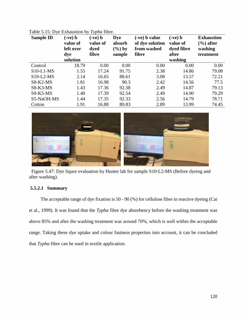
120

Table 5.15: Dye Exhaustion by Typha fibre.

Sample ID (-ve) b

value of

left over

dye

solution

(-ve) b

value of

dyed

fibre

Dye

absorb

(%) by

sample

(-ve) b value

of dye solution

from washed

fibre

(-ve) b

value of

dyed fibre

after

washing

Exhaustion

(%) after

washing

treatment

Control 18.79 0.00 0.00 0.00 0.00 0.00

S10-L1-MS 1.55 17.24 91.75 2.38 14.86 79.08

S10-L2-MS 2.14 16.65 88.61 3.08 13.57 72.21

S8-K2-MS 1.81 16.98 90.3 2.42 14.56 77.5

S8-K3-MS 1.43 17.36 92.38 2.49 14.87 79.13

S9-K5-MS 1.40 17.39 92.54 2.49 14.90 79.29

S5-NaOH-MS 1.44 17.35 92.33 2.56 14.79 78.71

Cotton 1.91 16.88 89.83 2.89 13.99 74.45

Figure 5.47: Dye liquor evaluation by Hunter lab for sample S10-L2-MS (Before dyeing and

after washing).

5.5.2.1 Summary

The acceptable range of dye fixation is 50 - 90 (%) for cellulose fibre in reactive dyeing (Cai

et al., 1999). It was found that the Typha fibre dye absorbency before the washing treatment was

above 85% and after the washing treatment was around 70%, which is well within the acceptable

range. Taking these dye uptake and colour fastness properties into account, it can be concluded

that Typha fibre can be used in textile application.

121

5.6 Hand Properties for Typha fibres

The oldest and most common process of transforming fibres into yarn is ring spinning. Twist

is inserted as the fibres leave the drafting unit. Fibre softness influences not only the fibre

mechanical properties such as coefficient of fabric surface friction, shearing properties, bending,

and draping properties, but also the yarn structure (twist). The finer the fibres, the greater the twist

of the yarn (Chattopadhyay & Sinha, 2007). A soft hand (feel of the fabric) is a desirable

characteristic of fabrics used in the apparel industry as it is the fabric feel which can influence a

customer’s purchase decision.

The hand property (softness) was measured using a standard AATCC evaluation procedure

5 (AATCC, 2010). In this method softness is evaluated using a rating scale of 1 (Least Soft) to 5

(Softest) and the evaluators were asked to evaluate based on compression, bending and surface.

The details of the evaluation method are given in Section 3.3.3. This rating may be used whether

or not the fibre can be processed in Cotton spinning machinery for yarn transformation.

At the beginning of the evaluation, evaluators were given eight standard fibre samples:

Cotton, wool, nylon, acrylic, silk, polyester, cannabis (virgin), and brassica (virgin). They were

then asked to rate the samples from 1 to 5 by touching, feeling, pressing and bending using thumb

and fourth finger. Once the evaluators had evaluated the standard samples, they were provided

with the four Typha samples: Typha leaf plant and three Typha fibre samples obtained by NaOH

treatment (S5-NaOH-MS), KOH treatment (S8-K3-MS) and LiOH treatment (S10-L3-MS). The

results of rating for standard and Typha samples are shown in Table 5.16(a).

It can be seen from Table 5.16(a) that silk fibre obtained the highest rating (4.8) while

polyester’s rating was 4.6. The ratings for Cotton, acrylic, wool and nylon were 4.0, 3.8, 3.0 and

2.0 respectively. The rating for virgin cannabis and virgin brassica were 1.0, and physical

122

examination showed that these two samples were very stiff. While the ranking was consistent for

the seven standard samples (the standard deviation ranged between 0.44 and 0.89), the rating for

acrylic fibre varied widely with a standard deviation of 0.81.

Among the Typha samples, the rating for Typha leaf plant was 1.0 while the ratings for

NaOH, KOH and LiOH treated fibre were 1.8, 2.8 and 1.6 respectively. All three ratings for Typha

fibres were lower than widely used textile fibres Cotton, wool, and polyester, however, the rating

of 2.8 (S8-K3-MS) was higher than nylon. A statistical analysis was employed to establish whether

these all fibres have significant difference in Table 5.16(a).

Table 5.16(a): Typha fibre softness grading with other common fibres.

Fibre Type Mean Std. Deviation Std. Error

Cotton 4.00 .000 .000

Wool 3.00 .000 .000

Nylon 2.00 .000 .000

Acrylic 3.80 .837 .374

Silk 4.80 .447 .200

Polyester 4.60 .548 .245

Cannabis (virgin) 1.00 .000 .000

Brassica (virgin) 1.00 .000 .000

Typha leaf (virgin) 1.00 .000 .000

Typha Fibre(S5-NaOH-MS) 1.80 .447 .200

Typha Fibre (S8-K3-MS) 2.80 .837 .374

Typha Fibre (S10-L3-MS) 1.60 .894 .400

F calculated 40.18

P-value 0.0005< (α =0.05)

Partial Eta squared (η) 0.902

Sample size (N) 5

A one-way between groups ANOVA was performed to compare the impact different types

of fibre had on hand feel properties rating. Twelve selected fibre with rating observations were

taken from observers (N=5) (in Appendix IX). The actual difference in the mean softness rating

123

between fibres was big effect size, (η =.902). There was a statistically difference between groups

as determined by one-way ANOVA (F (11, 59) = 40.176, p=.0005) in Table 5.23(a). A tukey post

hoc test revealed in pyramid shape that fibre hand feel properties were measured statistically

significance among twelve fibres shown in Table 5.16(b).

Cotton versus Typha hand feel properties exhibited S5-NaOH-MS (.0005<p), S10-L3-MS

(.0005<p) are statistically significant and S8-K3-MS (0.16<p) is not significant. Whereas Wool

vs. Typha showed S10-L3-MS, (.0005<p) was statistically significant, however, S8-K3-MS

(1.0<p) and S5-NaOH-MS, (0.16>p) were not significant. In Nylon vs. Typha no significant

difference was observed such as S5-NaOH-MS (1.0>p), S8-K3-MS (.323 >p) and S10-L3-MS

(.977>p). When comparing with Typha and Acrylic fibre, results showed a similar trend to Cotton;

for example S5-NaOH-MS (.0005<p) and S10-L3-MS (.0005<p) were significantly different in

their hand feel characteristics but S8-K3-MS (.086 >p) did not show any significant difference.

The evidence to reject the null hypothesis and conclude that all three Typha fibres were statistically

significant compared to polyester (S5-NaOH-MS (.0005 <p), S8-K3-MS (.0005<p), S10-L3-MS

(.0005<p) and silk (S5-NaOH-MS (.0005<p), S8-K3-MS (.0005<p), S10-L3-MS (.0005<p),

respectively. Virgin fibres including Cannabis, Brassica and Typha leaf plant possessed

homogeneous and have almost similar softness properties for S5-NaOH-MS (0.323 >p) and S10-

L3-M (0.735>p) were not significant, however, only S8-K3-MS (.0005<p) was significant (Table

5.16 (b)).

124

Table 5.16(b): Multi-comparisons using Tukey post hoc test results for the effect of hand feel properties on common fibres in pyramid

shape.

S8-K3-MS) vs.

S10-L3-MS

(.016 >p) S5-NaOH-MS vs.

S8-K3-MS

(.086 >p)

S5-NaOH-MS vs.

S10-L3-MS

(1.0 >p)

Typha leaf plant (v) (v)

vs.S5-NaOH-MS

(.323>p)

Typha leaf plant (v)

vs.S8-K3-MS

(.0005<p)


vs.S10-L3-MS

(.735 >p)

Brassica (v) vs.

Typha Fibre (v)

(1.0 >p)

Brassica (v) vs.

S5-NaOH-MS

(.323 >p)

Brassica (v) vs.

S8-K3-MS

(.0005 <p)

Brassica (v) vs.

S10-L3-MS

(.735 >p)

Cannabis (v) vs

Brassica (v)

(1.0 >p)

Cannabis (v) vs

Typha Fibre (v)

(1.0 >p)

Cannabis (v) vs

S5-NaOH-MS

(.323 >p)

Cannabis (v) vs

S8-K3-MS

(.0005 < p)

Cannabis (v) vs

S10-L3-MS

(.735 >p)

Polyester vs.

Cannabis (v)

(.0005 <p)

Polyester vs.

Brassica (v)

(.0005 <p)

Polyester vs.


(.0005 <p)

Polyester vs.

S5-NaOH-MS

(.0005 <p)

Polyester vs.

S8-K3-MS

(.0005<p)

Polyester vs.

S10-L3-MS

(.0005 <p)

Silk vs.

Polyester

(.977 >p)

Silk vs.

Cannabis (v)

(.0005 <p)

Silk vs.

Brassica (v)

(.0005 <p)

Silk vs. Typha

leaf plant (v)

(.0005 <p)

Silk vs.

S5-NaOH-MS

(.0005 <p)

Silk vs.

S8-K3-MS

(.0005 <p)

Silk vs.

S10-L3-MS

(.0005 <p)

Acrylic vs.

Silk

(.735 >p)

Acrylic vs.

Polyester

(.086 >p)

Acrylic vs.

Cannabis (virgin)

(.0005 <p)

Acrylic vs.

Brassica (virgin)

(.0005 <p)

Acrylic vs. Typha

leaf plant (v)

(.0005 <p)

Acrylic vs.

S5-NaOH-MS

(.0005 <p)

Acrylic vs.

S8-K3-MS

(.086 >p)

Acrylic vs.

S10-L3-MS

(.0005 <p)

Nylon vs.

Acrylic

(.0005<p)

Nylon vs.

Silk

(.0005<p)

Nylon vs.

Polyester

(.0005<p)

Nylon vs.

Cannabis (v)

(.086 >p)

Nylon vs.

Brassica (v)

(.086 >p)

Nylon vs.

Typha Fibre (v)

(.086 >p)

Nylon vs.

S5-NaOH-MS

(1.0>p)

Nylon vs.

S8-K3-MS

(.323 >p)

Nylon vs.

S10-L3-MS

(.977 >p)

Wool vs.

Nylon

(.086>p)

Wool vs.

Acrylic

(.323>p)

Wool vs.

Silk

(.002<p)

Wool vs.

Polyester

(.0005<p)

Wool vs.

Cannabis (v)

(.0005<p)

Wool vs.

Brassica (v)

(.0005<p)

Wool vs. Typha

leaf plant (v)

(.0005<p)

Wool vs.

S5-NaOH-MS

(0.16>p)

Wool vs.

S8-K3-MS

(1.0>p)

Wool vs.

S10-L3-MS

(.0005<p)

Cotton vs.

Wool

(.086 > p)

Cotton vs.

Nylon

(.0005<p)

Cotton vs.

Acrylic

(1.0 >p)

Cotton vs.

Silk (.977>p)

Cotton vs.

Polyester

(0.323>p)

Cotton vs.

Cannabis (v)

(.0005<p)

Cotton vs.

Brassica (v)

(.0005<p)

Cotton vs.

Typha

Leaf plant (v)

(.0005<p)

Cotton vs.

S5-NaOH-

MS

(.0005<p)

Cotton vs.

S8-K3-MS

(0.16>p)

Cotton vs.

S10-L3-MS

(.0005<p)

125

5.6.1 Summary

The statistical result shows that polyester and silk were not significant compared to Typha fibres,

which indicates Typha fibre cannot be processed on spinning machine alone. It appears that Typha

fibre sample S8-K3-MS is the best among Typha fibres because this sample is statistically similar

to Cotton, wool, nylon, acrylic, and better than cannabis and brassica. Considering this softness

grade of Typha, it could be possible to produce fibre blending with Cotton or wool or nylon or

acrylic with various blending ratio (for example 70:30, 60:40, Liu etal., 2011) to make suitable for

fibre spinning.

126

CHAPTER 6: CONCLUSION AND FUTURE WORK

Bast fibres, such as linum, brassica, cannabis and corchorus, are usually extracted using retting

methods, most commonly water, enzymes, or acid. Different treatments have been employed to

extract the fibres. Since the Typha plant grows in marshland areas, it demonstrated good resistance

to the extraction of starch, and it was hard to break the Typha cell walls through microbial attack

for retting. In this experiment, a water extraction method was applied for 90 days; however, it was

not suitable for isolating fibre from Typha stems. It has been observed that several attempts have

been made to extract fibres using enzymes, acid, and alcohol. None of these methods worked. In

our tests, the only extraction method that worked used alkali.

The fibres obtained from alkali retting were stiff and clustered together. During chemical

retting with LiOH, a higher yield of 66% was found compare to other bast fibres, but more fibre

protruding fibres were produced. The alkali method using KOH was more suitable than LiOH,

because of price and quality. It was noticed that alkali retting at low temperatures yields a fibre

with a gummy substance; better fibres are produced at higher temperatures of 80C to 95C. A

summary table (Table 6.1) has been prepared that indicates the fibre extraction process and

suitability of Typha fibres for textile and apparel applications.

127

Table 6.1: Summary for fibre extraction, yield (%), textile properties of Typha fibre and their

suitability in textiles and apparel applications

Parameters Results Comments

Retting

Water retting X Up to 100°C and three

months of treatment did not

produce any fibre.

Chemical retting

Acid retting X

Alcohol retting X

Enzyme retting X

Alkali √

Fibre yield (%) √ Yield (%) higher than all

other bast fibres

Physical properties

Length Yes Fibre length is shorter than

plant cut length

Diameter Yes Larger diameter variation

Microscopic nature Yes Round, rough, cells are

polygonal, have unique

crenelated structures.

Chemical properties Chemical compositions Cellulosic Wavenumber of 3433 cm−1

and 2920 cm−1 contain

cellulose peaks.

Moisture regain (%) Yes Average MR% is 10.9

Thermal properties

Thermal properties Yes Burning behavior similar to

cotton, heat resistance is

268.7 °C.

Chemical properties Dyeing with reactive dye Yes 80% dye exhaustion

Colourfastness to hot pressing Yes Performance rating:

Dry state: 3 to 4.5

Wet state: 2.5 to 4

Physical properties

Hand feel properties (*) Poor (2.8 out of 5), better

than nylon, however,

poorer than cotton and

polyester, need surface

modifications.

X – no fibre obtained; √: fibre obtained; (*) – suitable for textiles applications; Yes – properties

comparable with cotton and wool;

128

Typha fibres possess some potential textile properties with a diameter in the range of 10 to

14 µm, and the average cut length of 39 to 54 mm is similar to Cotton and wool fibre. Fourier

transform infrared spectrometer (FTIR) test values characterize that most important components

at the wave 3452.24 cm-1 for S10-L1-MS, are cellulose and hemicellulose. The wave length

1733.66 cm-1 for Typha plant indicates lignin and pectin content; the band for wax content at

2849.75 cm-1 was found to be a cellulosic fibre. As with Cotton and other cellulosic materials, this

group is dominant in Typha fibre.

There was no clear evidence that time or temperature of retting affects Typha fibre yield

(%), but it can be seen that the fibre yield (%) decreases with the increase in treatment time. On

the other hand, using similar treatment conditions in KOH at 95°C, the yield (%) is much lower

than the yield (%) at 80°C for most treatment hours, except for the 8 hours treated sample. It is

worth noting here that for the equivalent treatment conditions, the yield (%) using LiOH is much

higher than the KOH, particularly after 6 and 8 hours’ treatment. For example, after 6 hours’

treatment at 80°C, KOH treatment produced 35% fibre [S8-K3-MS, Figure 4.17(a)], whereas the

LiOH produced 56% fibre [S10-L3-MS, Figure 4.25 (a)], and after 8 hours’ treatment, KOH

treatment produced 15% fibre [S8-K4-MS, Figure 4.18 (a)] compared to 53% fibre [S10-L4-MS,

Figure 4.26 (a)] produced in LiOH, but the LiOH treatment is more costly.

While investigating visual characterization, it was discovered that the Typha plant consists

of different segments. There are some barriers for fibre extraction; one of them is that the Typha

inner core, hard woody stems increases fibre flakes (%). Plant type and seasonal cultivated plants

also affect extraction. Research found that fibre yield (%) may also be affected by plant

morphology. The flakes are fibre-like materials found in the fibre bundle from which fibres can be

separated by hand after immersing the stems in water, whereas, bark is a part of the hard/soft

129

woody stems. Fibre cannot be separated by hand from these stems after immersing in water, so the

fibre yield (%) varies widely in an otherwise good fibre bundle. It was found that, although initially

not known, the Typha plant can be categorized into three types: plants with a hard wood stem,

plants with a soft stem, and plants with no stem (only leaves). A suggestion to improve fibre yield

(%) and quality is to consider using no stem plants, as no leaf loss is required to get quality fibres.

Typha fibres represent a huge natural source of fibre with unique physical properties. If

these naturally abundant plants are used for textile and industrial applications, it will not only

benefit the grower or the farmer, but also increase overall economic activity.

Textile properties such as softness, individualization, moisture regain, thermal properties,

decomposition temperature, dyeability and colour fastness properties were evaluated. A textile

fibre should be soft for better acceptance in spinning systems; though bast fibres generally exhibit

a higher stiffness compared to other fibres. Typha demonstrated a softness rating of 2.8, softer than

brassica and cannabis, which had a softness rating of 1, and the synthetic fibre nylon, which had a

softness rating of 2. Moisture regain refers to wear comfort. Typha fibre exhibits an acceptable

range of moisture regain between 9.4 (%) and 12.7 (%). A textile fibre needs dye absorbability.

Typha fibre showed good dyeing properties in reactive blue dye, having dye exhaustion (%) of 72

to 79%, while the value for Cotton is 74.5%. During the burn test, Typha fibre displayed thermal

properties similar to Cotton fibre; Typha decomposition temperature was 268.7°C. The colour

fastness properties to hot pressing demonstrated good bearing power at different temperatures in

wet and dry conditions.

To make a quality fibre or yarn, one important condition is the softness of the fibre for ease

of spinning on the Cotton spinning system. However, Typha fibres obtained from the chemical

retting process are very stiff. Future research should focus on producing fine, flexible fibres. Bast

130

fibres are usually stiff because they consist of millions of microfibrils angled inside the cellulosic

fibres that are inversely proportional to stiffness (Tanushree & Chanana, 2016). Therefore, it is

necessary to further investigate mechanical properties to improve the knowledge of single fibre

tensile strength and flexural strength of Typha fibre. Though the softness grading of Typha fibre

was relatively low, it can be used as a blending fibre with other common fibres. Further study to

develop standard chemical retting parameters and establish the effect of chemical treatment on

fibre quality will be important. During Typha fibre extraction, different quality fibres (visual

appearance) were produced from different types (Hard stems, Soft stems and No stems) of plants.

Plant types / species or cultivars and the season of collection need to be investigated because the

level of fertility, temperature, plant density and irrigation could improve the fibre quality

(Tanushree & Chanana, 2016). Recently, bast fibres have received increased attention for their

unique characteristics. A suitable word for the new fibre could be “eco-bast” or “eco-leaf” fibre,

which could improve the sustainability of the textile industry by moving away from high input

crops to natural, low input feedstock.

131

REFERENCES

AATCC Test Method 133. (2009). Colorfastness to heat: hot pressing. In AATCC Technical

Manual NC, USA: American Association of Textile Chemists and Colorists, 215–216.

AATCC. (2010). Fabric hand: Guidelines for the subjective evaluation of. In AATCC Technical

Manual. NC, USA: American Association of Textile Chemists and Colorists, 85, 371–

373.

Abdullah, M., Rahmah, A.U., & Man, Z. (2010). Physicochemical and sorption characteristics of

Malaysian Ceiba pentandra (L.) Gaertn as a natural oil sorbent. Journal of Hazardous

Materials, 177, 683–691.

Academic Consultancy Training (ACT) project. (2013). Cattail an innovative solution for our

water challenges? Cattail Biorefinery. Project 1482

Acharya, S., Abidi, N., Rajbhandari, R., Meulewaeter, F. (2014). Chemical cationization of

Cotton fabric for improved dye uptake. Cellulose, 21, 4693-4706

Agrawal, B. K. (1988). Introduction to Engineering Materials. New Delhi: Tata McGraw-Hill,

52.

Aizenshtein, E. M. (1996). Current production and consumption of polyester fibres and yarns,

Fibre Chemistry, 28(5).

Akin, D.E., Condon, B., Sohn, M., Foulk, J.A., Dodd, R.B., & Rigsby, L.L. (2007). Optimization

for enzyme-retting of flax with pectate lyase. Industrial Crops and Products, 25, 136-

146.

Alawar, A., Hamed, A.M., & Al-Kaabi, K. (2009). Characterization of treated date palm tree

fiber as composite reinforcement. Composites Part B Engineering, 40, 601–606.

Ali, A. (2013). Surface modification of hemp fiber to improve spinning properties. Masters

132

thesis, University of Manitoba, 1-101.

Anderson, J. P., & Craig, W. J. (1984). Growing energy crops on Minnesota's wetlands: The

land use perspective. University of Minnesota Center for Urban and Regional Affairs, 84-

3.

ASTM International. (2008). Standard Practice for Conditioning and Testing Textiles. West

Conshohocken, United States. http://doi.org/10.1520/D1776-08E01.2

ASTM International. (2012). ASTM D2495-07 Standard Test Method for Moisture in Cotton by

Oven-Drying. Retrieved from https://doi-org.uml.idm.oclc.org/10.1520/D2495-07R12

ASTM International. (2016). ASTM D1776/D1776M-16 Standard Practice for Conditioning and

Testing Textiles. Retrieved from

https://doiorg.uml.idm.oclc.org/10.1520/D1776_D1776M-16

bacterial pectinolytic strains for improvement of hemp water retting. Euphytica, 140.47–54

Bednarz, C.W., Bridges, D.C., & Brown. S.M. (2000). Analysis of Cotton yield stability across

population densities. Agronomy Journal, 92,128-135.

Bidin, N., Zakaria, M.H., Bujang, J.S., & Aziz, N.A.A. (2015). Suitability of Aquatic plant

Fibres for Handmade Papermaking. International Journal of Polymer Science, 9.

http://dx.doi.org/10.1155/2015/165868

Blackburn, R.S. (Ed). (2005). Biodegradable and sustainable fibres. Cambridge: Woodhead. The

Textile Institute. 47.

Booth, J. E. (1968). Principles of textile testing: an introduction to physical methods of testing

textile fibres, yarns and fabrics. London, UK, Heywood Books, 111.

Brauer, D.S., Russel, C., Vogt, S., Weisser, J., & Schnabelrauch, M. (2008). Degradable

phosphate glass fiber reinforced polymer matrices: mechanical properties and cell

133

response. Journal of Materials Science: Materials in Medicine, 19,121–127. doi

10.1007/s10856-007-3147-x

Bridge, R.R., Meredith, W.R. Jr., & Chism, J.F. (1973). Influence of planting method and plant

population on Cotton (Gossypium hirsutum L.). Agronomy Journal, 65,104-109.

Cai, Y., Pailthorpe, M.T., & David, S.K. (1999). A new method for improving the dyeability of

Cotton with reactive dyes. Textile Research Journal, 69(6), 440- 446.

Cao, S., Dong, T., Xu, G., & Wang, F. (2016). Study on structure and wetting characteristic of

cattail fibers as natural materials for oil sorption. Environmental Technology, 37(24),

3193-3199, doi: 10.1080/09593330.2016.1181111

Cesar, N.R., Pereira-da-Silva, M.A., Botaro, V.R., & Menezes, A.J.D. (2015). Cellulose

nanocrystals from natural fiber of the macrophyte Typha domingensis: extraction and

characterization. Cellulose, 22:449–460.

Chattopadhyay, R., & Sinha, S. K. (2007). A study on spinning limits and yarn properties with

progressive change in yarn count in friction spinning. AUTEX Research Journal, 7(1).

Collier, B. J., & Epps, H. H. (1999). Textile testing and analysis. Upper Saddle River, New

Jersey: Prentice Hall.

Collier, B. J., Bide, M. J., & Tortora, P. G. (2009). Understanding textiles (7th ed.). Upper Saddle

River, New Jersey: Pearson Prentice Hall.

Cook, J.G. (2001). Handbook of textile fibres. Cambridge England: Woodhead. 2, 192 -193.

Cookson, P.G., & Slota, I.J. (1993). Hysteresis effects associated with the adsorption and

desorption of water by woven wool fabrics, Textile Research Journal, 63(9), 495-503.

Cotton fabric for improved dye uptake. Cellulose, 21, 4693–4706.

134

Curtis, S. (publ.) (1828). Curtis’s Botanical Magazine, Illustration of Corchorus olitorius, 55

(2), Tab. 2810, Image courtesy of Missouri Botanical Garden © 1995 -2009, http//:

www.botanicus.org

Dave, H., Lalita, L., Chandwani, N., Chauhan, N., & Nema, S.K. (2013). The removal of

impurities from gray Cotton fabric by atmospheric pressure plasma treatment and its

characterization using ATR-FTIR spectroscopy. The Journal of The Textile Institute, 105

(6), 586–596.

Dubbe, D. R., Garver, E. G., & Pratt, D. C. (1988). Production of cattail (Typha spp.) biomass in

Minnesota, USA. Biomass, 17(2), 79–104. https://doi.org/10.1016/0144-

4565(88)90073X.

Dubrovski, P. D. (Ed.) (2010). Woven fabric engineering, Rijeka, Croatia: Sciyo, 25.

Dungani, R., Karina, M., Subyakto, S. A., Hermawan, D., & Hadiyane, A., (2016). Agricultural

waste fibres towards sustainability and advanced utilization: A review. Asian Journal of

Plant Sciences, 15, 42-55. doi: 10.3923/ajps.2016.

Environment Canada. (2017). Environment Canada's weather - Environment and natural

resources - Weather information. Retrieved September 19, 2017, from

http://climate.weather.gc.ca/climate_data/hourly_data_e.html?StationID=27174&month=

6&day=11&timeframe=1&Year=2017&Month=6&Day=11&StartYear=1840&EndYear

=2017

Fahlgren, D. (2017). Genetic variation in common cattail (Typha latifolia) in southern Sweden.

M.Sc. Thesis, Swedish University of Agricultural Sciences.

Franck. R.R. (2005). Ramie. In: Bast and other plant fibres, Franck. R.R. (Ed.). Cambridge, UK:

Woodhead, 8-9.

https://doi.org/10.1016/0144-4565(88)90073X

https://doi.org/10.1016/0144-4565(88)90073X

135

Fu, J. (Ed.). (2013). Dyeing: Processes, techniques and applications, New York: Nova Science

ISBN: 978-1-62808-847-2, 1-18.

Gordon, S., & Hsieh, Y. L. (Eds.). (2007). Cotton: Science and technology (1st ed). Boca Raton,

USA: Woodhead, 68–102.

Grace, J. B., & Harrison, J. S. (1986). The biology of Canadian weeds: 73. Typha latifolia L.,

Typha angustifolia L. and Typha xglauca Godr. Canadian Journal of Plant Science,

66(2), 361-379.

Grosshans, R. E. (2014). Cattail (Typha spp.) biomass harvesting for nutrient capture and

sustainable bioenergy for integrated watershed management. PhD thesis, University of

Manitoba, 274.

Hamdaoui, M., Turki, S., Romdhani, Z., & Halaoua, S. (2013). Effect of reactive dye mixtures

on exhaustion values. Indian Journal of Fibre & Textile Research, 38, 405-409.

Hatch, K. L. (1993). Textile science. Saint Paul, Minneapolis: West.

Hearle, J.W.S., & Peters, R.H. (1963). Fibre structure. London: The Textile Institute

Butterworths.

Hoffmann, C. (1884). Botanischer Bilder- Atlas nach de Candolle’s Naturlichem

Pflanzensystem, with over 500 full-scale picture of plants on 85 fine colour plates and

explanatory text, Cocos nucifera, Plate 75, 431 a/b, J. Haffmann, Stuttgart, Germany,

online resource, Kurt Stueber (2003) http://caliban.mpiz-

koeln.mpg.de/stueber/hoffmann/index.html

Houlahan, J. E., Keddy, P. A., Makkay, K., & Findlay, C. S. (2006). The effects of adjacent land

use on wetland species richness and community composition. Wetlands, 26, (1), 79–96.

Hybl, J. (1975). Comparison of ring and open-end spinning. New York: Elsevier.

136

Jackowski, T., Chylewska, B., & Cyniak, D. (1999). Long staple Cotton – Technology of

spinning, GCA Cotton conference, Gdynia, Poland.

Judkins, G. (2008). Declining Cotton cultivation in Maricopa country, Arizona: An examination

of macro-and micro-scale driving forces. Yearbook of the Association of Pacific Coast

Geographers, 70(1), 70–95.

Judl, J., Hildén, M., Antikainen, S. R., Temmes, A., Kuisma, A.M., & Peck, P. (2016). The

renewal of forest-based industries needs to focus on environmental opportunities and

challenges. Conference paper, (10).

Kaczmar, J.W., Pach, J., & Burgstaller, C. (2011). The chemically treated hemp fibres to

reinforce polymers. Polimery, 56, 1112.

Kalia, S., Kaith, B. S., & Kaur, I. (Eds.). (2011). Cellulose fibres: Bio-and nano-polymer

composites, Berlin, Germany: Springer, ISBN: 978-3-642-17369-1, 3-42.

Kaushik, R. C. D., Tyagi, G. K., & Chatterjee, K. N. (1990). Contribution of fibre profile and

twist factor to flexural rigidity and elastic recovery of polyester fibre yarns, Indian

Journal Fibre & Textile Research, 200–201.

Khalid, R.H., Jawaid, M., Umer, R. (Eds.). (2014). Processing and properties of date palm fibers

and Its composites (1st ed). Springer-Verlag, 1–25. doi 10.1007/978-3-319-07641-6_1

Khan, M. R. I. (2016). Evaluation of brassica fibre for textile and spinning properties.

Unpublished manuscript, Department of Biosystems Engineering, University of

Manitoba, Winnipeg, Manitoba, Canada.

Kim, J. H., Rodgers, J., Delhom, C., & Cui, X. (2014). Comparisons of methods measuring fibre

maturity and fineness of upland Cotton fibres containing different degrees of fibre cell

wall development. Textile Research Journal, 84(15), 1622–1633.

137

King, D. (2007). Dyeing Cotton and Cotton products. In S. Gordon, & Y. L. Hsieh (Eds.),

Cotton: Science and Technology (1st ed). Boca Raton, USA: Woodhead, 353–380.

Kopke, V., & Lindberg, J. (1966). Steam-pressing of wool farbric: the influence of temperature

and moisture regain on the efficiency of pressing. Journal of the Textile Institute

(Transactions), 57(12), 551-573.

Kozłowski, R. M. (Ed.). (2012). Handbook of natural fibres. Cambridge, UK: Woodhead. 2,

219–253. http://doi.org/10.1533/9780857095510.2.219

Kozlowski, R. M. (2012a). Handbook of natural fibres (1st ed). Toronto, Canada: Woodhead, 2,

221–223. https://doi.org/10.1021/jf0617723

Kozlowski, R. M. (2012b). Handbook of natural fibres (1st ed), Cambridge, UK: Woodhead. 1,

64–65.

Kozlowski, R. M. (Ed.). (2012c). Handbook of natural fibres (1st ed), Cambridge, UK:

Woodhead . 1, 12.

Kozlowski, R. M. and Mackiewicz-Talarczyk, M. (2012). Handbook of natural fibres, (1st ed).

Cambridge,UK: Woodhead, 64-65.

Krässig, H. A. (1993). Cellulose, Structure, Accessibility and Reactivity. Philadelphia, USA:

Gordon and Breach Science.

Krowicki, R.S., Hemstreet, J.M., & Duckett, K.E. (1997). Determination of the 50% and 2.5%

span lengths and the uniformity ratio with the fibrograph, Journal of Textile Institute, 88

(Part I), 167-173.

Krus, M., Theuerkorn, W., Großkinsky, T., & Künzel, H. (2014). New sustainable and insulating

building material made of cattail. Nordic Symposium on Building Physics (NSB),10,

(156), 1252–1260. Retrieved from http://publica.fraunhofer.de/documents/N-

138

323927.html

Kumar, R.S. (2015). Process management in spinning. New York, Taylor & Francis Group.

Lawrence, C. A. (2003). Fundamental of spun yarn technology. Washington, New York: CRC

Press.

Lewin, S. M., & Pearce, E.M. (Eds.). (1998). Handbook of fibre chemistry. New York: Marcel

Dekker, 505-571.

Liggett, R.W., Hoffman, H. L., Tanquary, A.C., & Vail, S.L. (1968). Cross-linked cotton of high

moisture regain.Textile Research Journal, 38(4), 375-

387.https://doi.org/10.1177/004051756803800408

Li, X., Tabil, L.G., & Panigrahi,S. (2007). Chemical treatment of natural fibre for use in natural

fibre-reinforced composits. Journal of Polymer and the Environment, 15(1), 25-33.

Liu, L., Han, Y., & Zhang, X. (2011). Research on the spinnability of the renewable cattail fiber.

Advanced Material Research, 332- 334, 192-195.

Lord, P.R. (2003). Handbook of yarn production. Cambridge, England: Woodhead, 201.

Luamkanchanaphan, T., Chotikaprakhan, S., & Jarusombati, S. (2012). A Study of physical,

mechanical and thermal properties for thermal insulation from narrow-leaved cattail

fibres. APCBEE Procedia 1, 46 – 52.

Maizatul, O., Ruzaidi, G., Khalisanni, K., & Nazarudin, Z. (2012). Morphology and water

absorption analysis on single fibre and leaf of typha latifolia. Advanced Materials

Research, 576, 492-495.

Marques, G., Rencoret, J., Gutiérrez, A., & Del Río, J. C. (2010). Evaluation of the chemical

composition of different non-woody plant fibres used for pulp and paper manufacturing.

The Open Agriculture Journal, 4, 93-101.

139

Mohammed, L., Ansari, M.N.M., Pua, G., Jawaid, M., & Islam M.S.(2015). A review on natural

fibre reinforced polymer composite and its applications. International Journal of Polymer

Science, 2015(243947), 15, http://dx.doi.org/10.1155/2015/243947

Mather, R. R., & Wardman, R. H. (2015). The Chemistry of textile fibres (2nd ed). Cambridge,

UK: The Royal Society of Chemistry.

Meyers (1906).Groβes Konversations-Lexikon. Band 6. Faserpflanzen I und Faserpflanzen II.

Bibliographisches Institut, Wien/Leipzing, Austria/Germany, online resource, Editura

Gesellschaft fϋr Verlagsdienstleistungen mbH (2009), http://www.zeno.org.

Minotte, S. J., & Franck. R.R. (2005). Flax. In: Bast and other plant fibres, R. R. Franck (Ed.),

Cambridge, England: Woodhead, 159-160.

Mohanty, A.K., Manjusri, M., & Drzal, L.T. (2005). (Eds.). Natural fibres, Biopolymers and

Biocomposites. Florida, USA: CRC Press, 45 -50.

Moncrieff, R.W. (1963). Man-Made fibre (4th eds). London: Heywood. 19.

Montalvo, J., & G, Jr. (2005). Relationships between micronaire, fineness, and maturity. Part I.

Fundamentals. The Journal of Cotton Science, 9, 81–88.

Morton, W. E., & Hearle, J.W. S. (2008). Physical properties of textile fibres. Cambridge,

England: Woodhead, 134.

Muthu, S. (2018). Sustainable innovations in textile chemical processes. Singapore: Springer.

https://doi.org/10.1007/978-981-10-8491-1

Mussig, J. (Ed.). (2010). Function in nature. In: Industrial applications of natural fibres, West

Sussex, UK: John Wiley & Sons, 29.

Mwaikambo, Y. L., & Ansell, P. M. (2002). Chemical modification of hemp, sisal, jute, and

kapok fibers by alkalization. Journal of Applied Polymer Science. 84, 2222–2234.

140

Naveen, E., Venkatachalam, N., & Maheswaran, N. (2015). Alkali chemical treatment on the

surface of natural fiber. International Journal of Innovative Research in Science,

Engineering and Technology. 4 (4), 172-178.

Pabst, G. (ed.) (1887). Kohler’s Medizinal-Pflanzen in naturgetreuen Abbildungen mit kurz

erlauterndem Texte, Band I, Cannabis sativa L., Tafel 13, Organalzeichnungen von

Walther Muller in Gera, Gera- Untermhaus, Germany, Verlag von Fr. Eugen Kohler,

Image courtesy of Missouri Botanical Garden © 1995 -2009, http;//www.botanicus.org

Pandey, A. & Verma, R. K. (2018). Taxonomical and pharmacological status of Typha: A

Review. Annals of Plant Sciences, 7.3, 2101-2106.

Pandey, S.N. (2007). Ramie fibre: part II. Physical fibre properties. A critical appreciation of

recent developments. Textile progress. 19(4), 241.

Rashid, B., Yousaf, I., Haider, T., Rasheed, Z., Ali, Q., Javed, F., & Husnain, T. (2016).

Roadmap to sustainable Cotton production. Life Science Journal, 13(11), 41-48.

Rohlena, V. & Plisek, L. (1975). Open-end spinning. Elsevier, Amsterdam.

Rowland, S.P., Nelson, M. L., Welch, C.M., & Hebert, J.J. (1976). Cotton fiber morphology and

textile performance properties. Textile Research Journal, 46(3), 194- 214.

Roy, S., & Lutfar, L. B. (2012a). Bast fibres: ramie. In R. M. Kozlowski (Ed.), Handbook of

natural fibres: Properties and factors affecting breeding and cultivation. Cambridge,

UK: Woodhead, 1, 47–55.

Sana, R., Jaouadi, M., Khoffi, F., & Durand, B. (2016). Optimization of processing parameters

for extraction of typha stem fibers. International Journal of Applied Research on Textile,

4(2), 53-64.

Salit, M.S. (2014). Tropical natural fibre composites. Engineering Materials Singapore:

141

Springer. doi 10.1007/978-981-287-155-8_1

Sana, R., Mounir, J., & Slah, M. (2014). Study of structure and properties of tunisian typha leaf

fibres. International Journal of Engineering Research & Technology, 3(3), 539–546.

Sgriccia, N., Hawley, M. C., & Misra, M. (2008). Characterization of natural fibre surfaces and

natural fibre composites. Composites Part A: Applied Science and Manufacturing,

39(10), 1632–1637. https://doi.org/10.1016/j.compositesa.2008.07.007

Sharp, J. L. (B.S.). (2002). Managing cattail (Typha latifolia) growth in wetland systems.

Masters thesis, University of North Texas, 1-53.

Shore, J. (Eds.). (1995). Cellulosics dyeing, Manchester, UK: Society of Dyers and Colourists,

223-224.

Smith, C.W., & Coyle, G.G. (1997). Association of fibre quality parameters and within-boll

yield components in upland Cotton. Crop Science, 37, 1775-1779.

Smole, S.M., Hribernik, S., Kleinschek, S.K., & Kreže, T. (2013). Plant fibres for textile and

technical applications. Advances in Agrophysical Research, 369–397.

http://dx.doi.org/10.5772/52372

Sojda, R. S., & Solberg, K. L. (1993). Management and control of cattails. U.S. Fish and

Wildlife Leaflet. Waterfowl Management Handbook. 33.

http://digitalcommons.unl.edu/icwdmwfm/33

Sopit, V. (2007). Using cattails (Typha Latifolia) as a substrate for pleurotus ostreatus (Fr.)

kummer cultivation, 7(1), 218–221.

Sridach, W., & Paladsongkhram, R. (2014). Improvement of hardwood kraft paper with narrow-

leaved Typha latifolia L. fibre, cationic starch and asa. Cellulose Chemistry and

Technology, 48 (3-4), 375-383.

142

Stevulova, N., Cigasova, J., Estokova, A., Terpakova, E., Geffert, A., Kacik, F., Singovszka, E.,

& Holub, M. (2014). Properties characterization of chemically modified hemp hurds.

Materials, 7, 8131-8150; doi:10.3390/ma7128131.

Stout, E. E. (1960). Introduction to textiles. New York, USA: John Wiley & Sons, 26.

Sun, R.C., Lu, Q., & Sun, X.F. (2001). Physico-chemical and thermal characterization of lignins

from Caligonum monogoliacum and Tamarix spp. Polymer Degradation. Stability, 72,

229–238.

Tahir, P.M., Amel B. Ahmed, A.B., Saifulazry, S. O. A., & Ahmed, Z. (2011). Retting process of

some bast plant fibres and its effect on fibre quality: Review of bast fiber retting,

BioResources, 6(4), 5260-5281.

Tamburini, E., Gordillo, L. A., Perito, B, Candilo, M. D. (2004). Exploitation of bacteria

pectinolytic strains for improvement of hemp water retting. Euphytica, 140. 47-54

Tanushree, & Chanana, B. (2016). Characterization and mechanical properties of bast fibre.

International Journal of Home Science, 2(2), 291-295.

Taylor, M. A. (1972). Technology of textile properties. London: Forbes Publications, 7-10.

Thakur, V. K. (2015). Lignocellulosic polymer composites: Processing, characterization, and

properties. Massachusetts, USA: Scrivener.

Thomas, L. H., Forsyth, V. T., Sturcova, A., Kennedy, C.J., May, R.P., Altaner, C.M., Apperley,

D.C., Wess, T.J., & Jarvis, M.C. (2013). Structure of cellulose microfibrils in primary

cell walls from collenchyma. Plant Physiology, 161, 465–476,

Van der Werf, H. M. G., & Turunen, L. (2008). The environmental impacts of the production of

hemp and flax textile yarns. Industrial Crops and Products, 27, 1–10.

Vėjelienė, J., Gailius, A., Vėjelis, S., Vaitkus, S., & Balciunas, G. (2011). Evaluation of structure

143

influence on thermal conductivity of thermal insulating materials from renewable

resources. Materials Science, 17(2).

Wang, J.T., Zheng, Y.A., & Wang, A.Q. (2012). Effect of kapok fiber treated with various

solvents on oil absorbency. Industrial Crops and Products, 40, 178–184.

Wang, Y. (2006). Textile recycling. Cambridge UK: Woodhead.

Weatherall, I. L., & Coombs, B. D. (1991). Skin color measurements in terms of CIELAB color

space values. Invest Dermatol, 99(4), 468 - 473.

Williams, T., Hosur, M., Theodore, M., Netravali, A., Rangari, V., & Jeelani, S. (2011). Time

effects on morphology and bonding ability in mercerized natural fibers for composite

reinforcement. International Journal of Polymer Science, 2011, 1 – 9.

Wool, R. P., & Sun, X. S. (Eds.). (2005). Bio-Based Polymers and Composites. Amsterdam:

Elsevier.1–14. http://doi.org/10.1016/B978-012763952-9/50002-2

Wuzellaa, G., Mahendrana, A. R., Batgeb, T., Jurya, & Kandelbauerb. (2011). Novel, binder-free

fibre reinforced composites based on a renewable resource from the reed-like plant Typha

sp.ll, Industrial Crops and Products, 33, 683 – 689.

WWF Global (n.d.). Cotton farming, Cotton: A water wasting crop. Retrieved from

http://wwf.panda.org

Xiao, B., Sun, X. F., & Sun, R. (2001). Chemical, structural, and thermal characterizations of

alkali-soluble lignins and hemicelluloses, and cellulose from maize stems, rye straw, and

rice straw. Polymer Degradation and Stability, 74(2), 307–319.

https://doi.org/10.1016/S0141-3910(01)00163-X

Zeng, Y., Himmel, M.E., & Ding, S.Y. (2017).Visualizing chemical functionality in plant cell

walls. Biotechnol Biofuels, 10: 263,1 -16. doi 10.1186/s13068-017-0953-3

144

Zawani, Z., Abdullah, L. C., & Abdan, K. (2015). Characterization of kenaf fibre-retting

wastewater. International Journal of Science and Research, 4(6), 314–317.

Zhang, Y., Yang, S., Wu, J.Q., Yuan, T.Q., & Sun, R.C. (2014). Preparation and characterization

of lignocellulosic oil sorbent by hydrothermal treatment of Populus fiber. Materials, 7,

6733-6747; doi: 10.3390/ma7096733

Zheng, D. F., Qiu, X.Q., & Lou, H. M. (2005). The structure of lignin and its chemical

modification. Fine Chemicals, 22(4), 249–52.

145

Appendix I

Figure 4.15 (b): Typha fibre treated with alkali

(Sample ID: S8-K1-HS) for 2h/3%/80°C

Figure 4.15 (d): Typha fibre treated with alkali

(Sample: S8-K1-NS) for 2h/3%/80°C

Figure 4.16 (b): Typha fibre treated with

alkali (Sample: S8-K2-HS) for 4h/3%/80°C

Figure 4.15 (c): Typha fibre treated with

alkali (Sample: S8-K1-SS) for 2h/3%/80°C





146



Figure 4.17 (d): Typha fibre treated with

alkali (Sample: S8-K3-NS) for 6h/3%/80°C









147



Figure 4.19 (b): Typha fibre treated with alkali

(Sample: S9-K5-HS) for 2h/3%/95°C





Figure 4.20 (c): Typha fibre treated with alkali

(Sample: S9-K6-SS) for 4h/3%/95°C



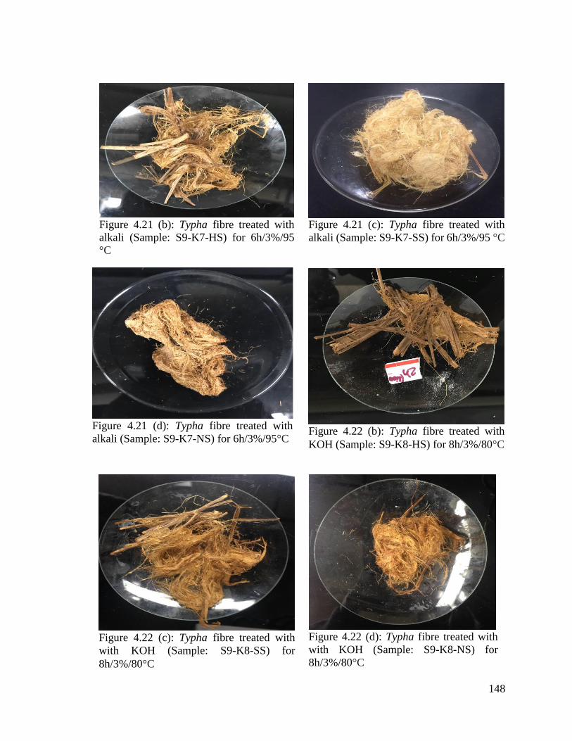
148




alkali (Sample: S9-K7-HS) for 6h/3%/95

°C


with KOH (Sample: S9-K8-NS) for

8h/3%/80°C


alkali (Sample: S9-K7-SS) for 6h/3%/95 °C


KOH (Sample: S9-K8-HS) for 8h/3%/80°C


with KOH (Sample: S9-K8-SS) for

8h/3%/80°C

149


LiOH (Sample ID: S10-L2-NS) for

4h/3%/80°C


LiOH (Sample: S10-L1-SS) for 2h/3%/80°C


LiOH (Sample: S10-L2-NS) for 2h/3%/80°C


LiOH (Sample: S10-L2-HS) for 4h/3%/80°C





150

Figure 4.26 (b): Typha latifolia L. fibre treated

with LiOH (Sample ID: S10-L4-HS) for

8h/3%/80°C

Figure 4.25 (c): Typha latifolia L. fibre treated

with LiOH (Sample ID: S10-L3-SS) for

6h/3%/80°C

Figure 4.26 (d): Typha latifolia L. fibre treated

with LiOH (Sample ID: S10-L4-NS) for

8h/3%/80°C


LiOH (Sample: S10-L3-NS) for 6h/3%/80°C





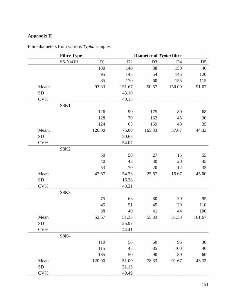
151

Appendix II

Fibre diameters from various Typha samples

Fibre Type Diameter of Typha fibre

S5-NaOH D1 D2 D3 D4 D5

100 140 38 150 40

95 145 54 145 120

85 170 60 155 115

Mean: 93.33 151.67 50.67 150.00 91.67

SD 43.10

CV% 40.13

S8K1

126 90 175 80 68

128 70 162 45 30

124 65 159 48 35

Mean: 126.00 75.00 165.33 57.67 44.33

SD 50.65

CV% 54.07

S8K2

50 50 27 15 55

40 43 30 20 45

53 70 20 12 35

Mean 47.67 54.33 25.67 15.67 45.00

SD 16.28

CV% 43.21

S8K3

75 63 80 30 95

45 51 45 20 110

38 40 41 44 100

Mean 52.67 51.33 55.33 31.33 101.67

SD 25.97

CV% 44.41

S8K4

110 58 60 95 30

115 45 85 100 40

135 50 90 80 60

Mean 120.00 51.00 78.33 91.67 43.33

SD 31.13

CV% 40.49

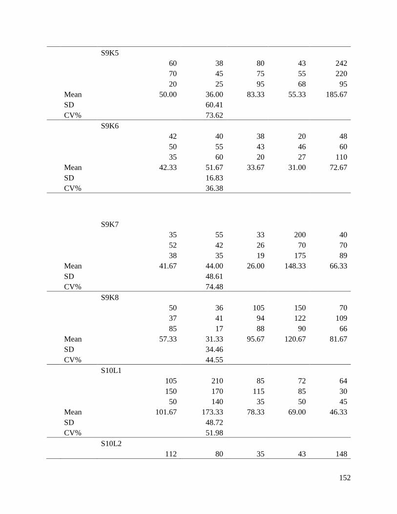
152

S9K5

60 38 80 43 242

70 45 75 55 220

20 25 95 68 95

Mean 50.00 36.00 83.33 55.33 185.67

SD 60.41

CV% 73.62

S9K6

42 40 38 20 48

50 55 43 46 60

35 60 20 27 110

Mean 42.33 51.67 33.67 31.00 72.67

SD 16.83

CV% 36.38

S9K7

35 55 33 200 40

52 42 26 70 70

38 35 19 175 89

Mean 41.67 44.00 26.00 148.33 66.33

SD 48.61

CV% 74.48

S9K8

50 36 105 150 70

37 41 94 122 109

85 17 88 90 66

Mean 57.33 31.33 95.67 120.67 81.67

SD 34.46

CV% 44.55

S10L1

105 210 85 72 64

150 170 115 85 30

50 140 35 50 45

Mean 101.67 173.33 78.33 69.00 46.33

SD 48.72

CV% 51.98

S10L2

112 80 35 43 148

153

93 65 55 48 135

144 120 30 37 96

Mean 116.33 88.33 40.00 42.67 126.33

SD 40.29

CV% 48.70

S10L3

160 120 54 33 80

140 107 96 30 50

125 70 39 20 46

Mean 141.67 99.00 63.00 27.67 58.67

SD 43.67

CV% 55.98

S10L4

21 130 33 12 17

19 150 16 17 26

45 111 22 25 35

Mean 28.33 130.33 23.67 18.00 26.00

SD 47.71

CV% 105.39

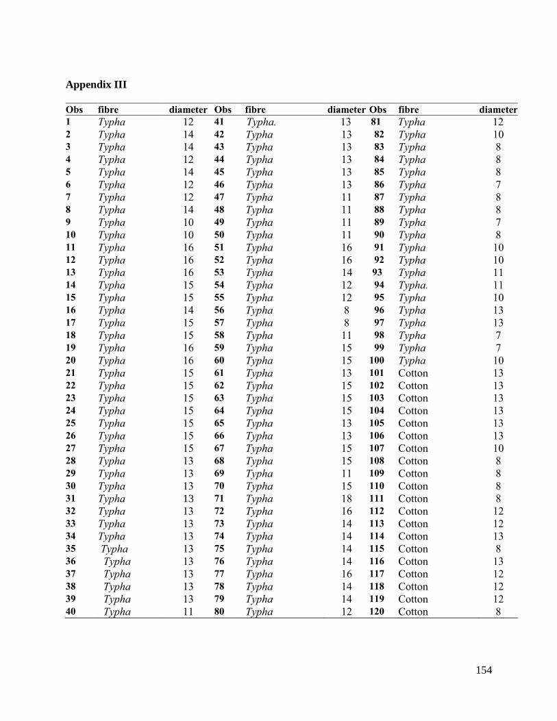
154

Appendix III

Obs fibre diameter Obs fibre diameter Obs fibre diameter 1 Typha 12 41 Typha. 13 81 Typha 12 2 Typha 14 42 Typha 13 82 Typha 10 3 Typha 14 43 Typha 13 83 Typha 8 4 Typha 12 44 Typha 13 84 Typha 8 5 Typha 14 45 Typha 13 85 Typha 8 6 Typha 12 46 Typha 13 86 Typha 7 7 Typha 12 47 Typha 11 87 Typha 8 8 Typha 14 48 Typha 11 88 Typha 8 9 Typha 10 49 Typha 11 89 Typha 7 10 Typha 10 50 Typha 11 90 Typha 8 11 Typha 16 51 Typha 16 91 Typha 10 12 Typha 16 52 Typha 16 92 Typha 10 13 Typha 16 53 Typha 14 93 Typha 11 14 Typha 15 54 Typha 12 94 Typha. 11 15 Typha 15 55 Typha 12 95 Typha 10 16 Typha 14 56 Typha 8 96 Typha 13 17 Typha 15 57 Typha 8 97 Typha 13 18 Typha 15 58 Typha 11 98 Typha 7 19 Typha 16 59 Typha 15 99 Typha 7 20 Typha 16 60 Typha 15 100 Typha 10 21 Typha 15 61 Typha 13 101 Cotton 13 22 Typha 15 62 Typha 15 102 Cotton 13 23 Typha 15 63 Typha 15 103 Cotton 13 24 Typha 15 64 Typha 15 104 Cotton 13 25 Typha 15 65 Typha 13 105 Cotton 13 26 Typha 15 66 Typha 13 106 Cotton 13 27 Typha 15 67 Typha 15 107 Cotton 10 28 Typha 13 68 Typha 15 108 Cotton 8 29 Typha 13 69 Typha 11 109 Cotton 8 30 Typha 13 70 Typha 15 110 Cotton 8 31 Typha 13 71 Typha 18 111 Cotton 8 32 Typha 13 72 Typha 16 112 Cotton 12 33 Typha 13 73 Typha 14 113 Cotton 12 34 Typha 13 74 Typha 14 114 Cotton 13 35 Typha 13 75 Typha 14 115 Cotton 8 36 Typha 13 76 Typha 14 116 Cotton 13 37 Typha 13 77 Typha 16 117 Cotton 12 38 Typha 13 78 Typha 14 118 Cotton 12 39 Typha 13 79 Typha 14 119 Cotton 12 40 Typha 11 80 Typha 12 120 Cotton 8

155

Obs fibre diameter Obs fibre diameter 121 Cotton 10 161 Cotton 14 122 Cotton 13 162 Cotton 15 123 Cotton 13 163 Cotton 15 124 Cotton 13 164 Cotton 13 125 Cotton 13 165 Cotton 15 126 Cotton 10 166 Cotton 15 127 Cotton 10 167 Cotton 13 128 Cotton 10 168 Cotton 13 129 Cotton 8 169 Cotton 15 130 Cotton 8 170 Cotton 13 131 Cotton 14 171 Cotton 10 132 Cotton 14 172 Cotton 12 133 Cotton 10 173 Cotton 13 134 Cotton 10 174 Cotton 14 135 Cotton 12 175 Cotton 13 136 Cotton 12 176 Cotton 13 137 Cotton 12 177 Cotton 12 138 Cotton 12 178 Cotton 10 139 Cotton 14 179 Cotton 10 140 Cotton 14 180 Cotton 10 141 Cotton 15 181 Cotton 12 142 Cotton 12 182 Cotton 12 143 Cotton 15 183 Cotton 14 144 Cotton 15 184 Cotton 14 145 Cotton 15 185 Cotton 12 146 Cotton 15 186 Cotton 14 147 Cotton 12 187 Cotton 12 148 Cotton 12 188 Cotton 14 149 Cotton 12 189 Cotton 9 150 Cotton 10 190 Cotton 12 151 Cotton 10 191 Cotton 13 152 Cotton 10 192 Cotton 13 153 Cotton 12 193 Cotton 15 154 Cotton 12 194 Cotton 15 155 Cotton 12 195 Cotton 15 156 Cotton 12 196 Cotton 13 157 Cotton 12 197 Cotton 13 158 Cotton 12 198 Cotton 13 159 Cotton 12 199 Cotton 13 160 Cotton 12 200 Cotton 13

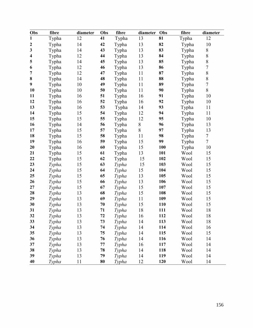
156

Obs fibre diameter Obs fibre diameter Obs fibre diameter 1 Typha 12 41 Typha 13 81 Typha 12

2 Typha 14 42 Typha 13 82 Typha 10 3 Typha 14 43 Typha 13 83 Typha 8 4 Typha 12 44 Typha 13 84 Typha 8 5 Typha 14 45 Typha 13 85 Typha 8 6 Typha 12 46 Typha 13 86 Typha 7 7 Typha 12 47 Typha 11 87 Typha 8 8 Typha 14 48 Typha 11 88 Typha 8 9 Typha 10 49 Typha 11 89 Typha 7 10 Typha 10 50 Typha 11 90 Typha 8 11 Typha 16 51 Typha 16 91 Typha 10 12 Typha 16 52 Typha 16 92 Typha 10 13 Typha 16 53 Typha 14 93 Typha 11 14 Typha 15 54 Typha 12 94 Typha 11 15 Typha 15 55 Typha 12 95 Typha 10 16 Typha 14 56 Typha 8 96 Typha 13 17 Typha 15 57 Typha 8 97 Typha 13 18 Typha 15 58 Typha 11 98 Typha 7 19 Typha 16 59 Typha 15 99 Typha 7 20 Typha 16 60 Typha 15 100 Typha 10 21 Typha 15 61 Typha 13 101 Wool 15 22 Typha 15 62 Typha 15 102 Wool 15 23 Typha. 15 63 Typha 15 103 Wool 15 24 Typha 15 64 Typha 15 104 Wool 15 25 Typha 15 65 Typha 13 105 Wool 15 26 Typha 15 66 Typha 13 106 Wool 15 27 Typha 15 67 Typha 15 107 Wool 15 28 Typha 13 68 Typha 15 108 Wool 15 29 Typha 13 69 Typha 11 109 Wool 15 30 Typha 13 70 Typha 15 110 Wool 15 31 Typha 13 71 Typha 18 111 Wool 18 32 Typha 13 72 Typha 16 112 Wool 18 33 Typha 13 73 Typha 14 113 Wool 18 34 Typha 13 74 Typha 14 114 Wool 16 35 Typha 13 75 Typha 14 115 Wool 15 36 Typha 13 76 Typha 14 116 Wool 14 37 Typha 13 77 Typha 16 117 Wool 14 38 Typha 13 78 Typha 14 118 Wool 14 39 Typha 13 79 Typha 14 119 Wool 14 40 Typha 11 80 Typha 12 120 Wool 14

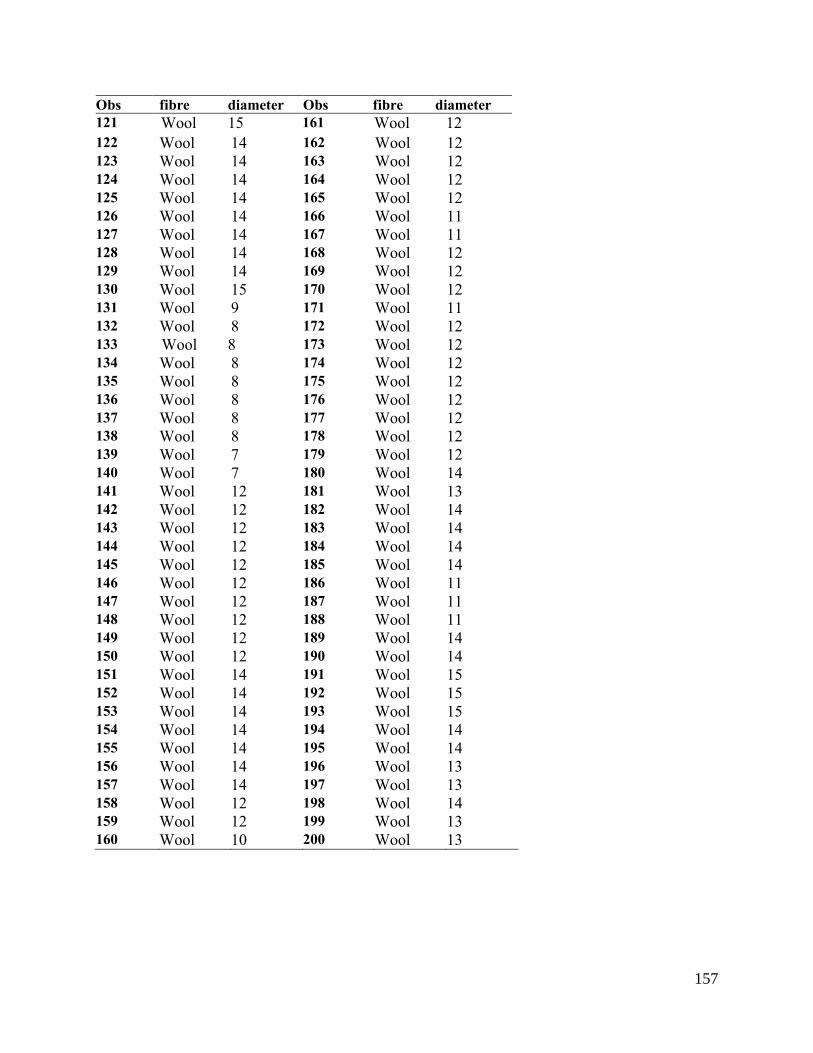
157

Obs fibre diameter Obs fibre diameter 121 Wool 15 161 Wool 12

122 Wool 14 162 Wool 12 123 Wool 14 163 Wool 12 124 Wool 14 164 Wool 12 125 Wool 14 165 Wool 12 126 Wool 14 166 Wool 11 127 Wool 14 167 Wool 11 128 Wool 14 168 Wool 12 129 Wool 14 169 Wool 12 130 Wool 15 170 Wool 12 131 Wool 9 171 Wool 11 132 Wool 8 172 Wool 12 133 Wool 8 173 Wool 12 134 Wool 8 174 Wool 12 135 Wool 8 175 Wool 12 136 Wool 8 176 Wool 12 137 Wool 8 177 Wool 12 138 Wool 8 178 Wool 12 139 Wool 7 179 Wool 12 140 Wool 7 180 Wool 14 141 Wool 12 181 Wool 13 142 Wool 12 182 Wool 14 143 Wool 12 183 Wool 14 144 Wool 12 184 Wool 14 145 Wool 12 185 Wool 14 146 Wool 12 186 Wool 11 147 Wool 12 187 Wool 11 148 Wool 12 188 Wool 11 149 Wool 12 189 Wool 14 150 Wool 12 190 Wool 14 151 Wool 14 191 Wool 15 152 Wool 14 192 Wool 15 153 Wool 14 193 Wool 15 154 Wool 14 194 Wool 14 155 Wool 14 195 Wool 14 156 Wool 14 196 Wool 13 157 Wool 14 197 Wool 13 158 Wool 12 198 Wool 14 159 Wool 12 199 Wool 13 160 Wool 10 200 Wool 13

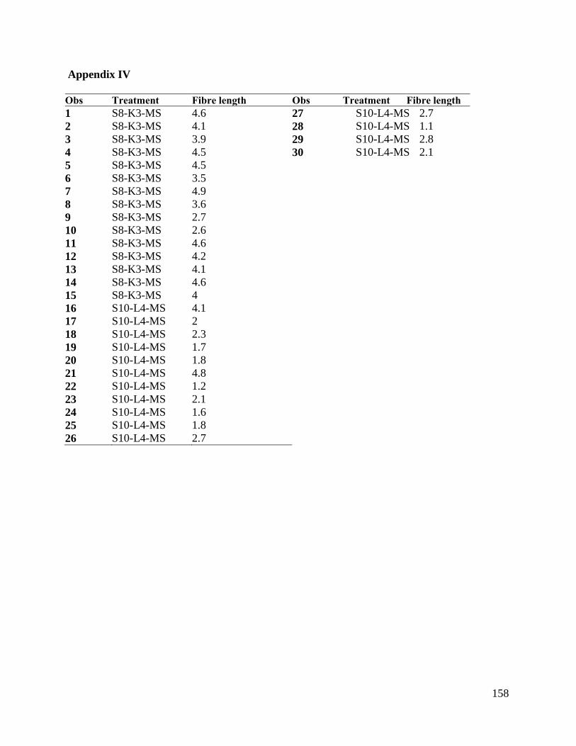
158

Appendix IV

Obs Treatment Fibre length Obs Treatment Fibre length

1 S8-K3-MS 4.6 27 S10-L4-MS 2.7

2 S8-K3-MS 4.1 28 S10-L4-MS 1.1

3 S8-K3-MS 3.9 29 S10-L4-MS 2.8

4 S8-K3-MS 4.5 30 S10-L4-MS 2.1

5 S8-K3-MS 4.5

6 S8-K3-MS 3.5

7 S8-K3-MS 4.9

8 S8-K3-MS 3.6

9 S8-K3-MS 2.7

10 S8-K3-MS 2.6

11 S8-K3-MS 4.6

12 S8-K3-MS 4.2

13 S8-K3-MS 4.1

14 S8-K3-MS 4.6

15 S8-K3-MS 4

16 S10-L4-MS 4.1

17 S10-L4-MS 2

18 S10-L4-MS 2.3

19 S10-L4-MS 1.7

20 S10-L4-MS 1.8

21 S10-L4-MS 4.8

22 S10-L4-MS 1.2

23 S10-L4-MS 2.1

24 S10-L4-MS 1.6

25 S10-L4-MS 1.8

26 S10-L4-MS 2.7

159

Appendix V

Figure 5.13: FTIR spectrum of extracted fibre from (a) Typha plant and (b) S8-K2;

(c) S5-NaOH; (d) S8-K3; (e) S10-L1; (f) S8-K4;

Figure 5.14(a): FTIR spectrum of Typha plant.

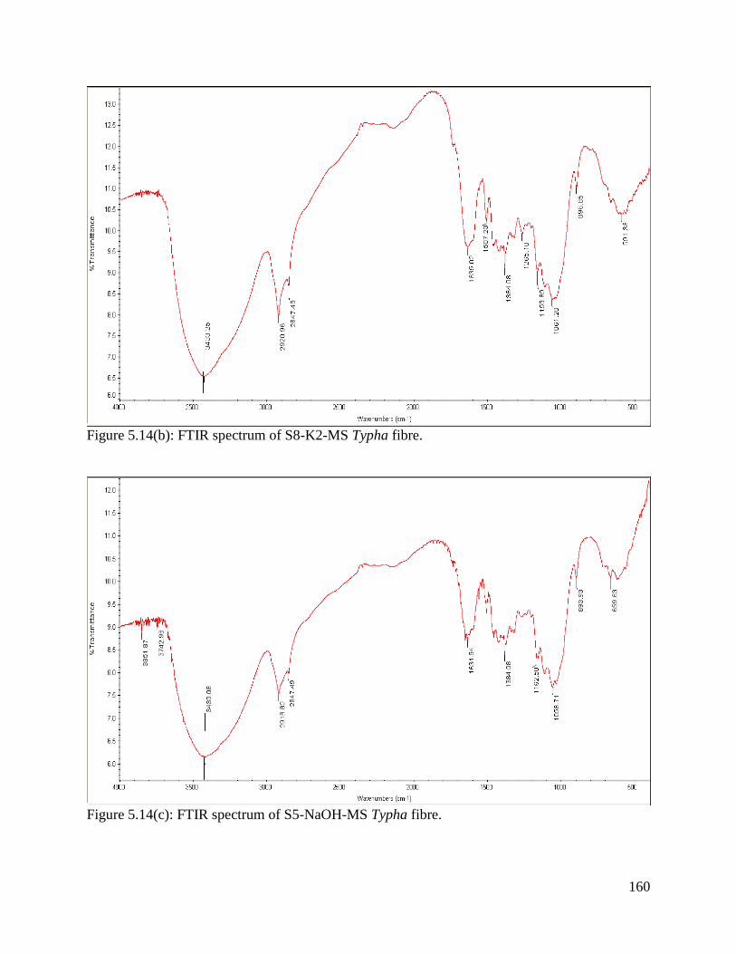
160

Figure 5.14(b): FTIR spectrum of S8-K2-MS Typha fibre.

Figure 5.14(c): FTIR spectrum of S5-NaOH-MS Typha fibre.

161

Figure 5.14(d): FTIR spectrum of S8-K3-MS Typha fibre.

Figure 5.14(e): FTIR spectrum of S10-L1-MS Typha fibre.

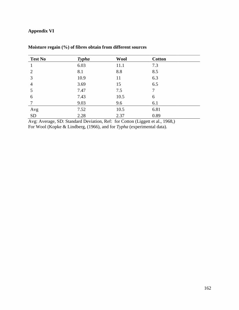
162

Appendix VI

Moisture regain (%) of fibres obtain from different sources

Test No Typha Wool Cotton

1 6.03 11.1 7.3

2 8.1 8.8 8.5

3 10.9 11 6.3

4 3.69 15 6.5

5 7.47 7.5 7

6 7.43 10.5 6

7 9.03 9.6 6.1

Avg 7.52 10.5 6.81

SD 2.28 2.37 0.89

Avg: Average, SD: Standard Deviation, Ref: for Cotton (Liggett et al., 1968,)

For Wool (Kopke & Lindberg, (1966), and for Typha (experimental data).

163

Appendix VII

Figure # 5.19 – 5.32 (a)

Holding time (10 minutes)

Figure # 5.19 – 5.32 (b)

Holding time (20 minutes)

Figure 5.19 (a) Figure 5.19 (b)

Figure 5.20 (a)

Figure 5.20 (b)

Figure 5.21 (a)

Figure 5.21 (b)

Figure 5.22 (a)

Figure 5.22 (b)

164

Figure 5.23 (a) Figure 5.23 (b)

Figure 5.24 (a)

Figure 5.24 (b)

Figure 5.25 (a)

Figure 5.25 (b)

Figure 5.26 (a)

Figure 5.26 (b)

165

Figure 5.27 (a)

Figure 5.27 (b)

Figure 5.28 (a)

Figure 5.28 (b)

Figure 5.29 (a)

Figure 5.29 (b)

Figure 5.30 (a)

Figure 5.30 (b)

166

Figure 5.31 (a)

Figure 5.31 (b)

Figure 5.32 (a)

Figure 5.32 (b)

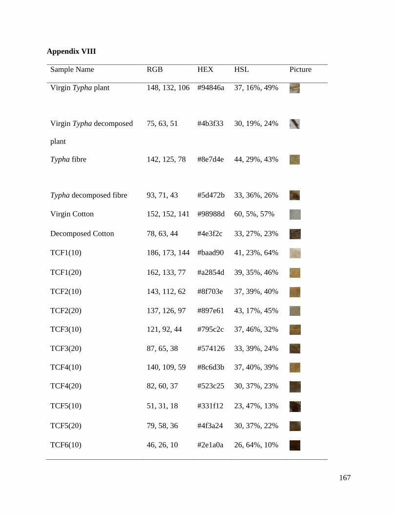
167

Appendix VIII

Sample Name RGB HEX HSL Picture

Virgin Typha plant 148, 132, 106 #94846a

37, 16%, 49%

Virgin Typha decomposed

plant

75, 63, 51

#4b3f33 30, 19%, 24%

Typha fibre 142, 125, 78

#8e7d4e 44, 29%, 43%

Typha decomposed fibre 93, 71, 43 #5d472b 33, 36%, 26%

Virgin Cotton 152, 152, 141 #98988d 60, 5%, 57%

Decomposed Cotton 78, 63, 44 #4e3f2c 33, 27%, 23%

TCF1(10) 186, 173, 144 #baad90 41, 23%, 64%

TCF1(20) 162, 133, 77 #a2854d 39, 35%, 46%

TCF2(10) 143, 112, 62 #8f703e 37, 39%, 40%

TCF2(20) 137, 126, 97 #897e61 43, 17%, 45%

TCF3(10) 121, 92, 44 #795c2c 37, 46%, 32%

TCF3(20) 87, 65, 38 #574126 33, 39%, 24%

TCF4(10) 140, 109, 59 #8c6d3b 37, 40%, 39%

TCF4(20) 82, 60, 37 #523c25 30, 37%, 23%

TCF5(10) 51, 31, 18 #331f12 23, 47%, 13%

TCF5(20) 79, 58, 36 #4f3a24 30, 37%, 22%

TCF6(10) 46, 26, 10 #2e1a0a 26, 64%, 10%

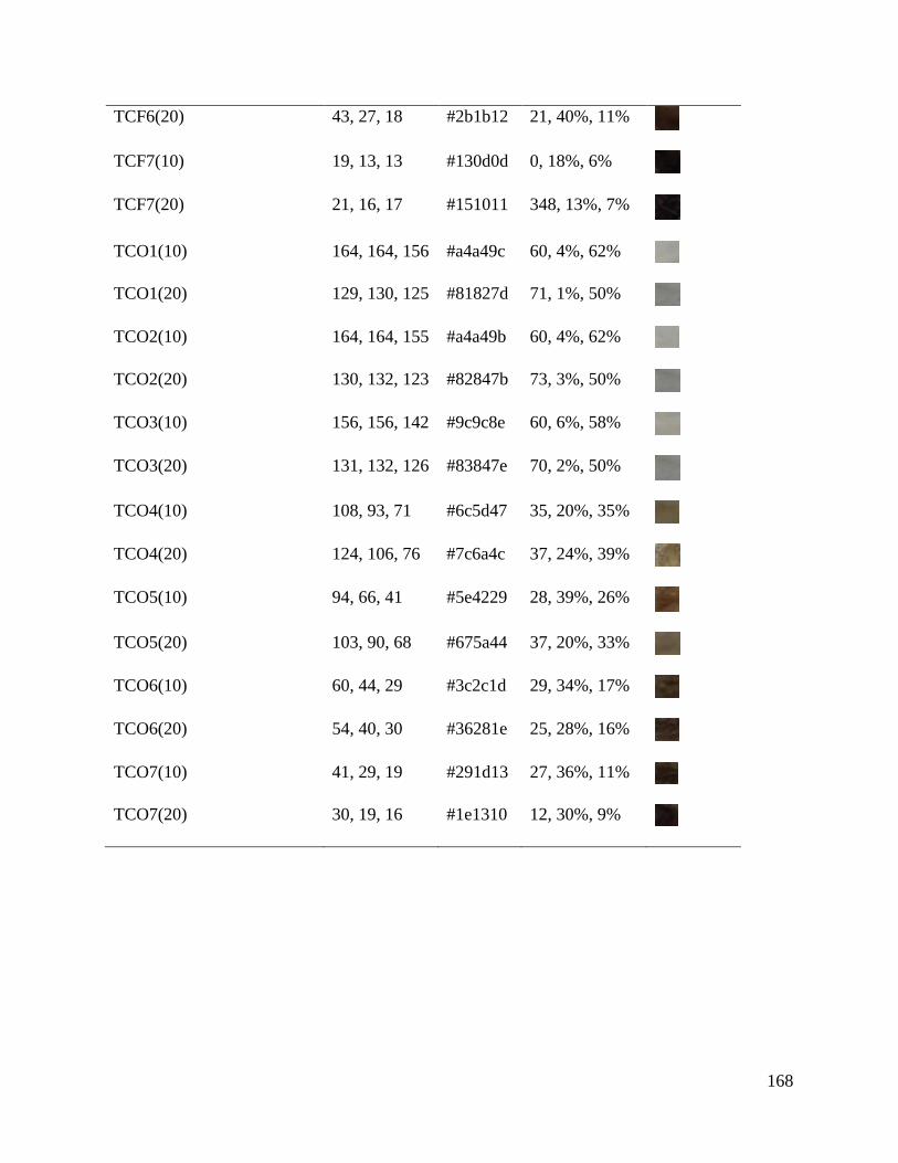
168

TCF6(20) 43, 27, 18 #2b1b12 21, 40%, 11%

TCF7(10) 19, 13, 13 #130d0d 0, 18%, 6%

TCF7(20) 21, 16, 17 #151011 348, 13%, 7%

TCO1(10) 164, 164, 156 #a4a49c 60, 4%, 62%

TCO1(20) 129, 130, 125 #81827d 71, 1%, 50%

TCO2(10) 164, 164, 155 #a4a49b 60, 4%, 62%

TCO2(20) 130, 132, 123 #82847b 73, 3%, 50%

TCO3(10) 156, 156, 142 #9c9c8e 60, 6%, 58%

TCO3(20) 131, 132, 126 #83847e 70, 2%, 50%

TCO4(10) 108, 93, 71 #6c5d47 35, 20%, 35%

TCO4(20) 124, 106, 76 #7c6a4c 37, 24%, 39%

TCO5(10) 94, 66, 41 #5e4229 28, 39%, 26%

TCO5(20) 103, 90, 68 #675a44 37, 20%, 33%

TCO6(10) 60, 44, 29 #3c2c1d 29, 34%, 17%

TCO6(20) 54, 40, 30 #36281e 25, 28%, 16%

TCO7(10) 41, 29, 19 #291d13 27, 36%, 11%

TCO7(20) 30, 19, 16 #1e1310 12, 30%, 9%

169

Appendix IX

Evaluation of softness grading with Typha and other common fibres.

Evaluators No

1 2 3 4 5

Name of

Fibres

Avg Std Yield

(%)

Cotton 4 4 4 4 4 4 0.0 N/A

Wool 3 3 3 3 3 3 0.0 N/A

Nylon 2 2 2 2 2 2 0.0 N/A

Acrylic 4 4 5 3 3 3.8 0.81 N/A

Silk 4 5 5 5 5 4.8 0.44 N/A

Polyester 5 5 5 4 4 4.6 0.54 N/A

Cannabis

(virgin)

1 1 1 1 1 1 0.0 12-15

Brassica

(virgin)

1 1 1 1 1 1 0.0 10-15

Typha

latifolia L.

(Virgin)

1 1 1 1 1 1 0.0 N/A

Typha

latifolia L.

(S5-NaOH-

MS)

2 2 2 1 2 1.8 0.44 56

Typha

latifolia L.

Fibre

(S8-K3-

MS)

3 3 4 2 2 2.8 0.83 35

Typha

latifolia L.

(S10-L3-

MS)

2 1 3 1 1 1.6 0.89 56

170

Appendix X

FORMULA

The pooled estimate of the sample standard deviation

S =√[(𝑛1−1)𝑆.𝐷.12+(𝑛2−1)𝑆.𝐷.22

𝑛1+𝑛2−2]

Calculate the value t from the equation

t = = 2.40 (Approx.)

Standard error of mean difference (1-2) = ( 𝑆1

2

𝑛1+

𝑆122

𝑛2)

Pooled Variance (Sp)2 =

(𝑛−1)𝑆12+(𝑛−1)𝑆2

2

𝑛1+𝑛2−2

Pooled Standard Deviation (Sp)2

Degree of freedom for Satterthwaite adjustment: 𝑑𝑓=

(𝑆1

2

𝑛1+

𝑆22

𝑛2)2

1

𝑛1−1(

𝑆12

𝑛1)2+

1

𝑛2−2(

𝑆22

𝑛2)2

T-test formula for unequal variances: tcal = ( 𝑋1 − 𝑋2 )

√𝑆1

2

𝑛1 +√

𝑆22

𝑛1

T-test formula pooled method: tcal = (𝑋1

− 𝑋2 )

√2𝑆𝑝

2

𝑛

Extraction Efficiency, Quality and Characterization of ...

Documents

Transcript of Extraction Efficiency, Quality and Characterization of ...