Extra stress tensor in fiber suspensions: Mechanics and ...
29
HAL Id: hal-01516400 https://hal.archives-ouvertes.fr/hal-01516400 Submitted on 30 Apr 2017 HAL is a multi-disciplinary open access archive for the deposit and dissemination of sci- entific research documents, whether they are pub- lished or not. The documents may come from teaching and research institutions in France or abroad, or from public or private research centers. L’archive ouverte pluridisciplinaire HAL, est destinée au dépôt et à la diffusion de documents scientifiques de niveau recherche, publiés ou non, émanant des établissements d’enseignement et de recherche français ou étrangers, des laboratoires publics ou privés. Public Domain Extra stress tensor in fiber suspensions: Mechanics and thermodynamics Miroslav Grmela, Amine Ammar, Francisco Chinesta To cite this version: Miroslav Grmela, Amine Ammar, Francisco Chinesta. Extra stress tensor in fiber suspensions: Me- chanics and thermodynamics. Journal of Rheology, American Institute of Physics, 2011, 55, pp.17-42. 10.1122/1.3523538. hal-01516400
Transcript of Extra stress tensor in fiber suspensions: Mechanics and ...

HAL Id: hal-01516400https://hal.archives-ouvertes.fr/hal-01516400
Submitted on 30 Apr 2017
HAL is a multi-disciplinary open accessarchive for the deposit and dissemination of sci-entific research documents, whether they are pub-lished or not. The documents may come fromteaching and research institutions in France orabroad, or from public or private research centers.
L’archive ouverte pluridisciplinaire HAL, estdestinée au dépôt et à la diffusion de documentsscientifiques de niveau recherche, publiés ou non,émanant des établissements d’enseignement et derecherche français ou étrangers, des laboratoirespublics ou privés.
Public Domain
Extra stress tensor in fiber suspensions: Mechanics andthermodynamics
Miroslav Grmela, Amine Ammar, Francisco Chinesta
To cite this version:Miroslav Grmela, Amine Ammar, Francisco Chinesta. Extra stress tensor in fiber suspensions: Me-chanics and thermodynamics. Journal of Rheology, American Institute of Physics, 2011, 55, pp.17-42.�10.1122/1.3523538�. �hal-01516400�
Extra stress tensor in fiber suspensions:
mechanics and thermodynamics
Miroslav Grmela1∗, Amine Ammar2,Francisco Chinesta3
1 Ecole Polytechnique de Montreal, C.P.6079 suc. Centre-ville,Montreal, H3C 3A7, Quebec, Canada
2 Laboratoire de Rheologie, INPG, UJF, CNRS (UMR 5520),1301 rue de la piscine, BP 53 Domaine Universitaire,
F-38041 Grenoble Cedex 9, France
3 EADS Corporate International Chair GeM,Ecole Centrale de Nantes BP 92101, 44321 Nantes, cedex 3, France
September 8, 2010
Abstract
Formulas expressing the extra stress tensor, �, in fiber suspensions interms of microstructural state variables are derived by using two typesof arguments: mechanical and thermodynamical. Results are comparedfor the distribution function (�) and the orientation tensor, �, playingthe role of state variables. The main results are the following: (i) In thethermodynamical analysis the formulas arise as compatibility conditionsbetween the time evolution of the fluid velocity and the time evolutionof the internal structure. (ii) A complete agreement among the formulasarising in mechanics and thermodynamics is seen only in kinetic theory(i.e. with � as the state variable) and only with the Chan-Terentjevmechanical formula. (iii) Theoretical arguments as well as numerical il-lustrations indicate that the larger is the role of the reversible part ofthe time evolution of the microstructure the larger is the difference inpredicted stresses (i.e. the formulas for � evaluated at solutions of themicrostructural equations) calculated with the thermodynamic and theDinh-Armstrong mechanical formulas.
1 Introduction
Let our interest in complex fluids be mainly directed towards their macroscopicflow behavior. The setting for their theoretical investigations has to include
∗corresponding author: e-mail: [email protected]
1

therefore classical hydrodynamics as its one (macroscopic) component. Thesecond (microscopic) component is needed because the complex fluids involvea microstructure (e.g. various suspended particles, macromolecules or mem-branes) that changes in time on the scale that is comparable to the time scaleof changes of hydrodynamic fields. The time evolution of the microstructurecannot be thus ignored even if our main interest is focused on the macroscopicflow.
In this paper we limit ourselves to isothermal and incompressible fluids. Theoverall fluid behavior is thus described only by the overall velocity fields �(�).By � we denote the position vector. The fluid density � and the temperature� are constants. Because of the convenience in both physical interpretationsand mathematical formulations, we shall use systematically the momentum field�(�) instead of the velocity field. If the only term in the energy that depends onthe velocity is the kinetic energy
∫�� 1
2��2 then the relation between � and � is
simply �(�) = ��(�). The state variable characterizing the microstructure willbe denoted by the symbol �(�). The field � can depend also on other variables(as for example � chosen in Section 2). The complete set of state variables usedin this paper (denoted formally by the symbol �) is thus
� = (�, �) (1)
Now we turn to the equations governing the time evolution of (1). As forthe momentum field �(�), the equation governing its time evolution is the localconservation law
∂�
∂�= −∇ ⋅
(��
�
)−∇�−∇ ⋅ � (2)
where � is the hydrostatic scalar pressure (determined by the incompressibilityrequirement), and � is the extra stress tensor. We shall consider in this paperonly symmetric extra stress tensors.
The complex fluids under investigation in this paper will be suspensions offibers. The microstructure characterized by �(�) is thus a characteristics of thedistribution of suspended fibers. Let the microscopic component of the settingof theoretical rheology be formally represented by the equation
∂�
∂�= �(�, �) + �(�, �) (3)
Advection of � with the flow is expressed in the term �(�, �). The physicsbehind the advection is the Stokes problem describing interaction of a fluidwith fibers suspended in it. The term � can also be seen as a term in which theexternal forcing on the microstructure (by imposing a flow) is expressed. Thedependence on � is such that �(−�, �) = −�(�, �). The second term �(�, �)represents dissipation. Most often � is independent of �. If it depends on �,the dependence is such that �(−�, �) = �(�, �). The physics that is behind theterm �(�) is best seen in the setting of thermodynamics. We shall discuss itbelow in Section 2.2.
2

Equations (2) and (3) are coupled in �(�) and �(�, �). The main objec-tive of this paper is to compare investigations, made by following two routes(mechanical and thermodynamical), of the relation between �(�) and �(�, �)in the context of fiber suspensions with two choices of � (� = one fiber distri-bution function, and � = an orientation tensor). The thermodynamical routeis moreover divided into two: classical nonequilibrium thermodynamics andGENERIC.
2 Kinetic theory
The internal structure (i.e. the distribution of suspended fibers) is chosen inthis section to be characterized by one fiber configuration space distributionfunction �(�,�), where � is the unit vector along the fiber.
2.1 Mechanics
Equation (2) has two mechanical interpretations. First, it is a local conservationlaw for the momentum �(�) (i.e. the right hand side of (2) is divergence of aflux), and second, it is a continuum version of Newton’s law. From the secondinterpretation we then see that � is a force acting on surface. We can thus find� by identifying the local surface forces acting on fibers. This is indeed the waythe expression for � has originally been derived. The mechanical approach tocalculating � in fiber suspensions has been initiated by Batchelor (1970),(1971)and later continued in Evans (1975), Dinh and Armstrong (1984) and Lipscombet al. (1988). The Dinh-Armstrong formula is a special case of the Lipscomb etal. formula. The most recent and the most complete analysis of the forces insidefiber suspensions has been made in Chan and Terentjev (2007). The expressionsderived by Chan and Terentjev will be denoted �(���ℎ�� )(�) and the expressionderived by Dinh and Armstrong �(���ℎ��)(�). The upper indices (���ℎ�� ) and(���ℎ��) denote the provenance of the formulas.
The advection term �(�) used in Chan and Terentjev (2007) is
�(�, �) = − ∂
∂��
(����
)− ∂
∂��(�̇� �) (4)
where�̇� = Ω���� + ������ − ����������, (5)
The second term on the right hand side (3) takes the form
�(�) =∂
∂��
(Λ (��� − ����)
∂�
∂��
)(6)
We use hereafter the summation convention �, �, � = 1, 2, 3, the tensors � and Ω
are respectively the symmetric and antisymmetric parts of the velocity gradient∇��
, � = �2−1�2+1 ; � is the fiber aspect ratio (fiber length to fiber diameter ratio).
3

The formula for the stress tensor �(���ℎ�� ) derived in Chan and Terentjev(2007) is the following:
�(���ℎ�� )�� = −�1
2
(∫��� ��
∂
∂��(Φ�) +
∫��� ��
∂
∂��(Φ�)
−2
∫���������
∂
∂��(Φ�)
)(7)
where
Φ =
∫��
�2
2�+ �������
∫��
∫�� � ln �, (8)
���� is the number density of the fibers, �� is the Boltzmann constant, � isthe temperature. We use hereafter the shorthand notation: ∂Φ
∂�(�) = Φ�(�)
and ∂Φ∂�
= Φ�. Moreover, we also use the symbol ∂ for both the ordinary
partial derivative and the Volterra functional derivative. For example, ∂Φ∂�(�) is
the Volterra functional derivative since Φ is a real valued function of a function�(�) and ∂Φ
∂��is an ordinary partial derivative of Φ that is a real valued function
of a finite number � of independent variables (�1, ...,�� ) where �� = �(��); � =1, 2, ..., � and (�1, ..., �� ) is a discretization of � ∈ ℝ
3.If we replace in (7) � with �������(�� � + 1) then indeed (7) is the sym-
metric part of the stress tensor appearing in Eq.(64) in Chan and Terentjev(2007). We are choosing to write the formula in the form (7) because it appearsin this way in thermodynamics (in the following Section 2.2). We shall see thatthe quantity Φ has the physical interpretation of free energy.
The formula for the fiber contribution to the extra stress tensor derived byDinh and Armstrong (1984) is the following:
�(���ℎ��)�� = 2������������ (9)
where ����� =∫�� �������� �(�,�), �� is the matrix viscosity, and �� is a
dimensionless parameter called the particle number that represents the relativeimportance of the fibers, � is the symmetric velocity gradient.
We shall compare the formulas (7), (9) and also other formulas derived belowin Sections 2.2 and 2.3 in Section 2.4.
2.2 Thermodynamics
In this subsection we consider externally unforced fiber suspensions. The experi-mental observation on which we shall concentrate is the approach to equilibriumstates at which the behavior of suspensions is seen to be well described by clas-sical equilibrium thermodynamics. We look for a structure of the equationsgoverning the time evolution of the state variables (1) that will guarantee thatsolutions of the equations agree with the above experimental observation.
We begin with a short preparation. We say that Eqs.(2), (3) are time re-versible if the inversion of the sign of the time � is compensated by the trans-formation (�, �) → (−�, �) (i.e. a simultaneous application of � → −� and
4

(�, �) → (−�, �) leaves (2), (3) invariant). If the simultaneous application of�→ −� and (�, �) → (−�, �) does not leave (2), (3) invariant, the two equationsare called time irreversible.
First, we turn to Eq.(2). We split � into two parts:
� = �(+) + �(−) (10)
where �(+) is invariant with respect to (�, �) → (−�, �), and �(−) changes itssign if (�, �) → (−�, �) is applied. We see now that Eq.(2) with � = �(+) istime reversible.
Next, we turn to Eq.(3). Since � is assumed to depend on � in such a waythat � remains invariant with respect to the transformation � → −�, Eq.(3)without � is time irreversible and Eq.(3) without � is time reversible (since weassume that �(−�, �) = −�(�, �)).
Now, we are in position to present the thermodynamic argument that willlead us to an expression for the extra stress tensor �. The argument is thesame for both choices of the internal state variables (i.e. for both �(�,�) and�(�)). We present it therefore below with �(�,�) representing both choices. LetΦ(�, �) be the free energy. We choose it in such a way that Φ(�, �) = Φ(−�, �).We recall its role in the time evolution. As a consequence of the observedapproach of externally unforced fluids to equilibrium states (denoted (�, �)��) ,the following inequality holds
�Φ
��=
∫��
[��
∂��∂�
+
∫��Φ�
∂�
∂�
]≤ 0 (11)
The free energy Φ plays thus the role of the Lyapunov function for the ap-proach. The equilibrium states (�, �)��, reached as � → ∞, are the state atwhich Φ reaches its minimum and are therefore solutions to Φ� = 0, Φ� = 0)[we use hereafter the shorthand notation: ∂Φ
∂� = Φ� and ∂Φ∂�
= Φ�] Moreover,
Φ evaluated at the equilibrium state (�, �)�� becomes the equilibrium thermo-dynamic free energy determining the equilibrium thermodynamic properties ofthe fluid under consideration.
We shall replace (11) by a somewhat stronger statement:
(�Φ
��
)(−)
=
∫��
[��
∂(���� + ���� + �(+)�� )
∂��+
∫��Φ��
]= 0 (12)
(�Φ
��
)(+)
=
∫��
[−Φ��
∂�(−)��
∂��+
∫��Φ��
]< 0 (13)
It is clear that Eqs.(12) and (13) imply (11) (since ���
= (���
)(+) +(���
)(−)) but(11) does not, in general, imply (12),(13).
The stress tensors arising from Eqs.(12) and (13) will be hereafter denoted�(�ℎ) in order to indicate their provenance.
5
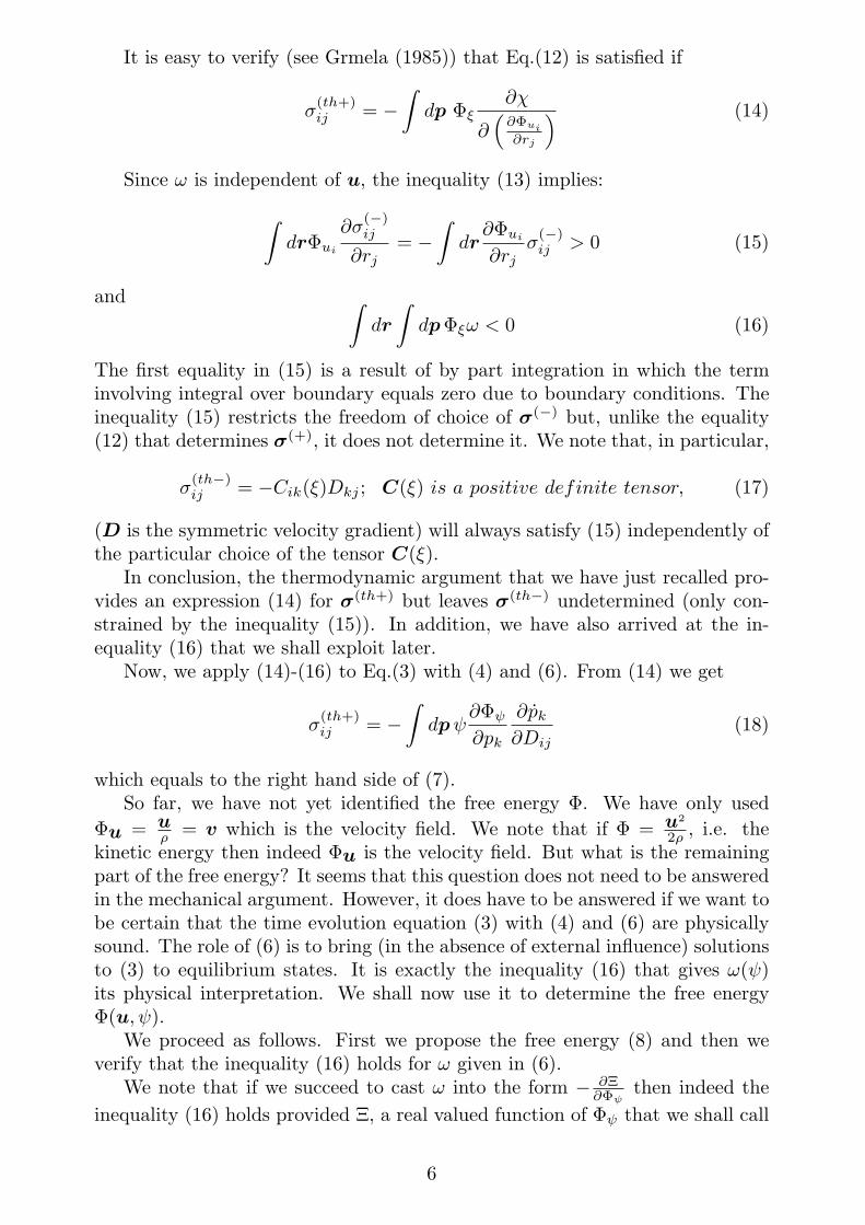
It is easy to verify (see Grmela (1985)) that Eq.(12) is satisfied if
�(�ℎ+)�� = −
∫�� Φ�
∂�
∂(∂Φ��
∂��
) (14)
Since � is independent of �, the inequality (13) implies:
∫��Φ��
∂�(−)��
∂��= −
∫��∂Φ��
∂���(−)�� > 0 (15)
and ∫��
∫��Φ�� < 0 (16)
The first equality in (15) is a result of by part integration in which the terminvolving integral over boundary equals zero due to boundary conditions. Theinequality (15) restricts the freedom of choice of �(−) but, unlike the equality(12) that determines �(+), it does not determine it. We note that, in particular,
�(�ℎ−)�� = −���(�)��� ; �(�) �� � �������� �������� ������, (17)
(� is the symmetric velocity gradient) will always satisfy (15) independently ofthe particular choice of the tensor �(�).
In conclusion, the thermodynamic argument that we have just recalled pro-vides an expression (14) for �(�ℎ+) but leaves �(�ℎ−) undetermined (only con-strained by the inequality (15)). In addition, we have also arrived at the in-equality (16) that we shall exploit later.
Now, we apply (14)-(16) to Eq.(3) with (4) and (6). From (14) we get
�(�ℎ+)�� = −
∫���
∂Φ�∂��
∂�̇�∂���
(18)
which equals to the right hand side of (7).So far, we have not yet identified the free energy Φ. We have only used
� = ��
= � which is the velocity field. We note that if Φ = �2
2� , i.e. thekinetic energy then indeed Φ� is the velocity field. But what is the remainingpart of the free energy? It seems that this question does not need to be answeredin the mechanical argument. However, it does have to be answered if we want tobe certain that the time evolution equation (3) with (4) and (6) are physicallysound. The role of (6) is to bring (in the absence of external influence) solutionsto (3) to equilibrium states. It is exactly the inequality (16) that gives �(�)its physical interpretation. We shall now use it to determine the free energyΦ(�, �).
We proceed as follows. First we propose the free energy (8) and then weverify that the inequality (16) holds for � given in (6).
We note that if we succeed to cast � into the form − ∂Ξ∂Φ�
then indeed the
inequality (16) holds provided Ξ, a real valued function of Φ� that we shall call
6

a dissipation potential, is such that Ξ(0) = 0, Ξ reaches its minimum at 0, andΞ is convex in a neighborhood of 0 [recall that if Ξ is a real valued function of� ∈ ℝ satisfying the properties listed above than indeed ��Ξ
��> 0].
Now we identify the dissipation potential Ξ (see Grmela (2008)):
Ξ(Φ�) =
∫��
∫��(ℛΦ�)�
1
2�Λ(ℛΦ�)� , (19)
where Λ > 0 is a coefficient and (ℛΦ�)� = (�× ∂∂�Φ�)� ; × denotes the vector
product.We have thus proven that (8) is the free energy (implicitly) present in the
kinetic equation (3), (4), (6), and (7). The first term in (8) is the kinetic energyand the second term is the entropy multiplied by −1.
We end this subsection with three observations.Observation 1 According to the virtual work principle (Doi (1983), Doi
and Edwards (1986) p.70, see also Feng et al. (2000), Wang (2002), Sircar andWang (2009)) the variation of the microstructural contribution to the free energydensity (i.e. the variation of the second term on the right hand side of (8)) equalsthe work done to the material by the elastic stress (i.e. in our notation �(+)).We note now that this is in fact an alternative physical interpretation of theequality (12). Indeed, the first term on the right hand side of (12) (after makingby parts integration and using the expression � = �− ��Φ��
−∫���Φ�, where
� defined by Φ =∫��� for the hydrostatic pressure �) becomes the work done
to the material by the elastic stress (i.e. �(+)) multiplied by −1. The secondterm is clearly the variation of the microstructure contribution to the free energydensity. We thus conclude that the virtual work principle is equivalent to therequirement (expressed in (12)) that the total free energy remains unchangedduring the reversible time evolution.
Observation 2 We have seen that the thermodynamic argument (i.e. therequirement that solutions of the time evolution equations agree with the ex-perimental observation constituting the basis of classical equilibrium thermo-dynamics) does leave the irreversible part �(−)(�,�) of the extra stress tensorundetermined. We have seen that, for example, any expression of the form(17) is admissible. We shall now argue that �(−)(�,�) = 0. The physicsexpressed in �(−)(�,�) is the physics of dissipative processes taking place insuspensions. But we have already taken such processes into account in the term�(�) in Eq.(3) governing the time evolution of the microstructural state vari-able �(�,�). Assuming that the dissipative processes are expressed completelyin �(�), we have no physical basis (inside the thermodynamic argument) forconstructing �(−)(�,�). We thus conclude that (inside the thermodynamicargument) �(−)(�,�) = 0. We shall discuss this point further in Section 2.4.Observation 3 The split of the time evolution into the reversible and irre-
versible parts depends on the choice of the morphological state variable � in (1).In other words, the split of the time evolution into the reversible and irreversibleparts is level dependent. By a level of description we mean the way we regardthe system under consideration. For example, the choice of the morphological
7

state variable that we have made in this section corresponds to a more micro-scopic (i.e. involving more details) level than the level corresponding the choicethat we shall make in Section 3. We shall illustrate the level dependence ofthe reversible-irreversible splitting of the time evolution on two examples. Letthe complex fluid under investigation be composed, for the sake of simplicityof the illustration, of only point particles. In the first example we choose � toconsist of the position coordinates and velocities of all particles composing thefluid. The time evolution in this case is completely time reversible, there is notime irreversible part. In particular, all the interactions among the particlesenter the time reversible part. In the second example we choose the morpho-logical state variable to be the one particle distribution function, either in theconfiguration space (i.e.� = �(�)) or in the phase space (i.e. � = �(�,�), where� is the velocity). Let the particles interact among each other and let the in-teraction be expressed in a mean-field type potential � (��)(�). In the case of� = �(�,�), this potential enters into the time reversible part (in the form of∂∂�
(� ∂�
(��)(�)∂�
)) as well as into the time irreversible part. On the other hand,
in the case of � = �(�), the mean-field potential is absent in the time reversiblepart.
2.3 GENERIC
As in the previous subsection, we consider externally unforced fiber suspensions.Our objective is to identify the structure of the time evolution equations guar-anteeing that their solutions agree with the experimentally observed approachto equilibrium. The structure identified in this subsection will be richer thatthe one identified in the previous section. In addition to requiring the compati-bility with thermodynamics we shall require that the mechanics (Newton’s law)does not enter only Eq.(2) but also Eq.(3). In this subsection we shall combinemechanics and thermodynamics into a single formalism addressing both Eqs.(2)and (3).
To begin with, we have to choose a formulation of mechanics that is ap-propriate for making the combination. Among several possible mathematicalformulations of Newton’s law, we shall choose the Hamiltonian formulation. Ithas been first used in the context of hydrodynamics by Clebsch (1895). It ap-pears to be the most convenient for expressing the advection term �(�, �) in (3)as a result of the mechanical interaction of the fluid with an obstacle and forcombining mechanics with thermodynamics.
Clebsch (1895) and Arnold (1966) have shown that the Euler equation, i.e.Eq.(2) with � = 0, can be cast into the form
��
��= {�,�}(�) ℎ���� ��� ��� � (20)
where � is a sufficiently regular real valued function of � and � is the energy
8
∫���
2
2� (i.e. (8) with the second term missing) and
{�,�}(�) =
∫����
(∂���
∂�����
− ∂���
∂�����
)(21)
is a Poisson bracket in which the kinematics of continuum (i.e. the Lie groupof transformations ℝ
3 → ℝ3) is expressed.
Now, we supplement the momentum field �(�) with the fiber distributionfunction �(�,�) and ask the question of what is the Poisson bracket expressingkinematics of (�(�), �(�,�)). If we assume that � is passively advected (Liedragged) by � then the bracket is given by (see Grmela (1988))
{�,�}(�,�) = {�,�}(�) +
∫��
∫�� �
(∂��∂��
���− ∂��∂��
���
)
+�
∫��
∫�� ���(��� − ����)
(∂��∂��
∂���
∂��− ∂��∂��
∂���
∂��
)
(22)
The mechanical content of the time reversible part of the evolution of (�(�), �(�,�))is now expressed by requiring that the governing equations have still the form(20) (expressing the mechanical content of the Euler equation) but with {�,�}(�)replaced by {�,�}(�,�) and � replaced by the total energy. The explicitform of the governing equations (including the explicit formula for the extrastress tensor) emerges now in the following calculations. The left hand side
of (20) is written as∫�����(�)
∂��(�)∂�
+∫��
∫����(�,�)
∂�(�,�)∂�
. The righthand side of (20) is written (with the use of by parts integration) in the form∫�����(�)(∙)�+
∫��
∫����(�,�)(∙∙), where (∙)� and (∙∙) represent the expres-
sions obtained in the calculations. Since Eq.(20) is required to hold for all �,
we obtain ∂��(�)∂�
= (∙)� and∂�(�,�)∂�
= (∙∙). These equations are the same asEqs.(2),(3) with �(�, �) given in (4), the term �(�) missing, and � given in(7). The extra stress tensor � arising in this analysis will be hereafter denotedby the symbol �(�������) to denote its provenance. We have thus shown that�(�ℎ+) = �(�������+). This result is not surprising if we realize that (20)implies �Φ
��= {Φ,Φ} = 0 and that this equality served as a basis (see (12)) on
which (7) was obtained in Section 2.2.Having addressed the time reversible part of the evolution, we now proceed
to the time irreversible part. Here we join the previous subsection. The onlyrequirement is the compatibility with thermodynamics expressed by the inequal-ity �Φ/�� ≤ 0 required to hold during the time evolution. As in the previoussubsection, we note that if
(∂�
∂�
)
���
= − ∂Ξ
∂Φ�(23)
(∂�
∂�
)
���
= − ∂Ξ
∂Φ�(24)
9

are the equations governing the time irreversible evolution then indeed �Φ/�� ≤0 holds provided Ξ(Φ�,Φ�) is a potential, called a dissipation potential, satisfy-ing: (i) Ξ(0, 0) = 0, (ii) Ξ reaches its minimum at (0, 0), and (iii) Ξ is convex ina neighborhood od (0, 0). As we have seen at the end of Section 2.2, the choice(19) of the dissipation potential corresponds to the choice (6) of � (see Eq.(3)).
The potential (19) is not however the only dissipation potential for which
− ∂Ξ∂Φ�
= ∂∂��
(Λ (��� − ����) ∂�∂��
)and �Φ/�� ≤ 0. For example, if we choose
Ξ(Φ�,Φ�) =
∫��
∫��(ℛΦ�)�
1
2�Λ(ℛΦ�)� +
1
2
∫����������� (25)
(��� = 1/2(∂�Φ��
+ ∂�Φ��
), ∂� = ∂/∂��, and � is a positive definite ten-
sor) then we still satisfy the inequality �Φ/�� ≤ 0 and the time evolution of(�(�), �(�,�) is governed by Eq.(2) (with � = �(+) +�(−), where �(+) is givenin (7) and �(−) in (17)) and Eq.(3) with � and � given in (4),(6). We thusconclude that the stronger requirement that we have used in this subsectionstill leaves the part �(−) undetermined.
We end this subsection with three observations.Observation 1 Exactly the same argument as the one introduced in Obser-
vation 2 in the previous section leads us again to �(−) = 0. Section 2.4 belowprovides additional arguments in favor of this conclusion.Observation 2 If we combine the Hamiltonian reversible time evolution
presented above with the dissipative time evolution generated by �(�) (ex-pressed with the help of the dissipation potential discussed in Section 2.2) insuch a way that the inequality (11) is guaranteed, we arrive at a time evolu-tion generated by equations that have started to appear in Dzyaloshinski andVolovick (1980) and later in Grmela (1984), Kaufman (1984), Morrison (1984),Beris and Edwards (1994). An abstract equation representing an appropriatelycombination of the reversible Hamiltonian and the irreversible dissipative vectorfield has been called GENERIC in Grmela and Ottinger (1997) and Ottinger andGrmela (1997). GENERIC has been then further developed in Grmela (2001),(2002), (2004), (2010) and in a different direction in Ottinger (1998),(2005). Thecompatibility of the reversible and irreversible time evolution is essentially a re-quirement guaranteeing satisfaction of (12) and (13). Beside this constraint,the irreversible part of the time evolution remains undetermined. This thenmeans that, like in the preceding section, the irreversible part �(�������−)
of the extra stress tensor remains undetermined (except that (13) is requiredto hold). The geometrical interpretation in which the time evolution generatedby GENERIC becomes a continuous sequence of Legendre transformations (seeGrmela (2010)) provides an additional insight into the coupling of the reversibleand irreversible time evolutions.Observation 3 The third observation is about the bracket (22). It can
easily be verified that (22) is a Poisson bracket only for � = 1 and � = −1with the tensor ∂��/∂� transposed. Otherwise, the Jacobi identity is notverified. We can understand this observation as follows: From the mathematicalpoint of view, it is well known (see the concept of the semi direct product in
10

e.g. Marsden and Ratiu (1999)) that the scalar �(�,�) has to be passivelyadvected (in other words, Lie dragged) in order that the extended space withcoordinates (�(�), �(�,�) be equipped with a Poisson bracket extending thePoisson bracket (21). The extended Poisson bracket is then the bracket (22).From the physical point of view, the advection (in our case Eq. (5) ) is a result,as we have already mentioned in the text following Eq. (3), of solving theStokes problem. The passive advection that ie expressed in (22) corresponds toa special solution to the Stokes problem, namely to the solution in which the flowof the fluid remains completely undisturbed by the presence of suspended fibers.This special solution can be considered to be an acceptable approximation ofthe actual solution only for fibers with special shapes like an infinitely thin fiber
and an infinitely thin plate. Indeed, if we recall that � = �2−1�2+1 where � is the
fiber aspect ratio (fiber length to fiber diameter ratio) then � = 1 correspondsto the infinitely thin fiber and � = −1 to an infinitely thin plate.
The question arises as to whether it is possible to consider the case � ∕= ±1inside GENERIC. Below, we shall briefly indicate how the non-passive characterof the advection can be incorporated into the dissipative part of the GENERICstructure. Instead of the kinematics (22), we shall regard a fiber as a rigid rod.The state variables (�(�), �(�)) (for the sake of simplicity we shall limit our-selves in this observation to homogeneous suspensions, i.e. � is independent of�) are replaced by (�(�), �(�),�(�)), where �(�) is the angular momentum.The kinematics of these state variables is expressed (see Grmela and Lafleur(1998)) by the Poisson bracket
{�,�}(���) =
∫��
∫���
[(∂��∂��
���− ∂��∂��
���
)
+��
(∂���
∂�����
− ∂���
∂�����
)+��(�� �� )�
+����
((�� × ∂���
∂�)� − (�� × ∂���
∂�)�
)](26)
where (� × �)� = �������� is the vector product of two vectors �, and �; � isthe alternating tensor; �� = ����
∂����
is the vorticity; and �� = �����������. The
same calculations as those that we sketched in the text following (22) lead us to
∂�
∂�=∂(��× Φ� )�
∂��(27)
We note now that if we let to dissipate the angular momentum �(�) in sucha way that Φ� approaches rapidly −1
2�� then, as an approximation, we canreplace in the first equation of (27) Φ� by −1
2��. The resulting equationbecomes equivalent to the kinetic equation Eq.(3) with the term � missing andthe term �(�, �) given by (4) and (5).
11

2.4 Comparison of different formulas for the extra stress
tensor
The results obtained above in this section imply
�(���ℎ�� )(�) = �(�ℎ)(�) = �(�������)(�) (28)
�(���ℎ��)(�) ∕= �(���ℎ�� )(�) (29)
and�(���ℎ��)(�) ∕= �(�ℎ)(�) (30)
The first equality in (28) provides an additional argument (in addition to theone presented in Observation 2 in Section 2.2) for �(�ℎ−) = �(�������−) = 0.The inequalities (29) and (30) arise due to the following two reasons: forces andmorphology of the microstructure are investigated on different levels of descrip-tion, and the stresses are investigated in driven systems and not in externallyunforced systems considered in Sections 2.2 and 2.3. We now discuss these tworeasons in some detail.Stresses and the microstructure investigated on different levels of
description We note that the extra stress tensor that is actually observed inexperiments (we shall call it hereafter a predicted stress) is �(�∣��.(3)), whereby �∣��.(3) we denote solutions to Eq.(3) with a given �. The predicted stressis thus independent of � and depends only on the symmetric velocity gradient�. Let now the process of finding the solution to Eq.(3) be regarded as agradual process representing, from the physical point of view, a gradual descendto more macroscopic levels of description, and from the mathematical pointof view a gradual restriction of the functions �(�,�) to submanifolds of theoriginal state space. The well known example of the restricted submanifold is thelocal Maxwellian distribution function and its Chapman-Enskog deformations(see more in Grmela (2010)) providing a passage from the phase space kinetictheory to hydrodynamics. Another example is the van Wiechen-Booij (1971)configuration space distribution function �(�) ∼ exp (�������), where the tensor� is proportional to the inverse of the orientation tensor �̊, providing a passagefrom the configuration space kinetic theory to the orientation tensor theory.
Let the distribution function � restricted to such submanifold (we can alsosee it as a partial solution) be denoted by �∣
�̃�.(3)). If �(�) is replaced by
�(�∣�̃�.(3)
) then clearly both formulas will give exactly the same predicted
stresses. In general, we can think of an infinite number of �∣�̃�.(3)
representing
an exact partial solutions to Eq.(3) and thus an infinite number of formulas forthe extra stress tensor, all looking very differently but all implying exactly thesame predicted stresses.
The formula �(�∣�̃�.(3)
) can also be seen as being directly derived on a more
macroscopic (i.e. less detailed) level than the level on which the distributionfunction � serves as the microstructural state variable. The state variable usedon the more macroscopic level is � restricted to the manifold on which � =
12

�∣�̃�.(3)
). We can thus regard the formula �(���ℎ��) as obtained in this way.
The microstructure equation (3) can indeed be, in principle, investigated ona level of description and the formulas for the extra stress tensor on anotherdifferent level of description. If however such a route is taken, then the mainproblem is the compatibility, i.e. the problem of guaranteeing that the physicsput into the derivation of the microstructure equation (3) is the same as thephysics put (on another level of description) into the derivation of the formulafor the extra stress tensor. From the mathematical point of view, this problemis then the problem of proving that �̃ for which �(�ℎ)(�̃) = �(���ℎ��)(�) isindeed �∣
�̃�.(3), i.e. a partial solution of Eq.(3).
Can we identify �̃ for which �(���ℎ�� )(�̃) = �(���ℎ��)(�)?. It has beennoted in Grmela (2008) that �(���ℎ�� )(�) turns into �(���ℎ��)(�) if � in�(���ℎ�� ) is replaced by
�̃(�) = �������� exp (�������) (31)
which is indeed an approximate solution of (3) corresponding to small symmetricvelocity gradients �. The better (31) approximates solutions to (3) the closerare the the predicted stresses calculated from both formulas.
Externally unforced versus driven suspensions What is observed inrheological investigations are responses of fluids to external forces. The externalforces are typically imposed overall flows and the responses are observed in bothstresses and the microstructural morphology. The advection term �(�, �) inEq.(3) represent the external influence. Given �, solution to (3) provides theresponse of the internal structure. In order to obtain the stresses induced bythe externally imposed flow, the internal structure obtained as a solution to(3) has to be inserted into the formula �(�) for the extra stress tensor. Twoquestions arise: (i) different external forces require different levels of descriptionto investigate the responses, (ii) can the formulas �(�) derived in Section 2.2and 2.3 for externally unforced fluids (from the requirement that such fluidsapproach equilibrium states) be used in rheological investigations? The firstquestion is clearly out of the scope of this paper. Our starting point is themicrostructural equation (3), we do not investigate its domain of applicability.We only note that there are always external forces for which any given level ofdescription (i.e. any given choice of � and Eq.(3)) will appear to be inadequatefor discussing the fluid response. As for the second question, we see that theformulas for the extra stress tensor derived on the basis of the compatibilitywith thermodynamics do not have indeed a universal applicability in rheology.Ideally, the formulas for � should be obtained from a mechanical analysis, i.e.from an analysis of forces inside the suspension. Such analysis will, in general,different for different external forces. Moreover, we have to require that thephysics involved in the analysis of the forces should always be the same as theone involved in the derivation of the microstructural equation. The fact thatthe Chan-Terentjev mechanical formula for the extra stress tensor is the sameas the formula derived from thermodynamics is a strong indication of a ratherbroad applicability of thermodynamic considerations in rheology.
13

Comparison with results of rheological measurements Predicted stresses(formulas for the stress tensor evaluated at solutions to the microstructural equa-tions) that can be compared with results of experimental observations dependon both the microstructural equation (3) and the expression for the extra stresstensor �(�). Comparison with experiments does not therefore contribute toanswering the question asked in this paper (i.e. the question: given microstruc-tural equations, what is the corresponding to it expression for the extra stresstensor).Numerical illustration We shall now solve the microstructural equation
(3) numerically and compare the predicted stresses implied by different for-mulas �(�). The discussion presented above in this subsection indicates thecomplexity of the issues involved in the comparison. Consequently, the nu-merical investigation, however detailed, will not really represent a substantialcontribution to the discussion. We shall therefore limit ourselves to showing,for selected values of the material parameters involved in (3), that the predictedstresses are indeed different for different formulas but the difference is not large.
In the numerical illustration presented below we assume that the distributionfunction �(�), where ∣�∣ = 1, is independent of the position vector �, the velocitygradient of the imposed flow is
∇� =
⎛⎝
−� 0 �0 � 00 0 0
⎞⎠ (32)
where � and � are constants.We begin the numerical solution by passing to a week form of the kinetic
theory equation. We use as degrees of freedom the nodal values of the distri-bution function over a triangular tetellation of the unit sphere (which is herethe configurations space of all possible 3D orientations). The model used in thecalculations involves about 2500 degree of freedom. Then we consider a par-ticular velocity gradient given by By using an implicit time integration schemewe calculate at each time step the distribution function. The initial state isgiven by the isotropic orientation i. e. �(�) = 1/4�. Simulations are done for� = 0.1, � = 1 and three values 0.005, 0.05, 0.5 of the parameter Λ. Figures 1, 2and 3 depict the distribution function �(�), the orientation tensor � calculatedas the second moment of the distribution function (i.e. ��� =
∫�������(�)),
and predicted stress calculated by using the formulas �(���ℎ��) and �(���ℎ�� ).
14

��
����
�
���
�
��
�
���
����
�
���
�
�
��� �� � ��� ��� Λ � ���� � � ���� � � �
�
�
����
����
����
����
����
����
���
����
����
���
� �� �� �� �� ����
����
���
����
���
����
��
�� �
���
!�" �# $� %&' ��� Λ � ���� � � ���� � � �
��
()*+,-.-*/,-+,0/)
122133124
� �� �� �� �� �������
�����
�
����
���
����
���
����
!�" �# $� %&' ��� Λ � ���� � � ���� � � �
��
5-)+00-+,0/)
σ22�σ
33 6 78σ24 6 78
σ22�σ33 6 9:σ24 6 9:
Figure 1: Distribution function �(�), corresponding to it orientation tensor� =
∫�����(�), and predicted stresses � for � = 0.1, � = 1 and Λ = 0.5
15
��
����
�
���
�
��
�
���
����
�
���
�
�
��� �� � ��� ��� Λ � ����� � � ���� � � �
�
�
����
���
����
���
����
� �� �� �� �� ����
���
���
���
���
���
���
���
�! �" #� $%& ��� Λ � ����� � � ���� � � �
��
'()*+,-,).+,*+/.(
011022013
� �� �� �� �� �������
�
���
���
���
���
���
���
�! �" #� $%& ��� Λ � ����� � � ���� � � �
��
4,(*//,*+/.(
σ11�σ22 5 67
σ13 5 67
σ11�σ22 5 89σ13 5 89
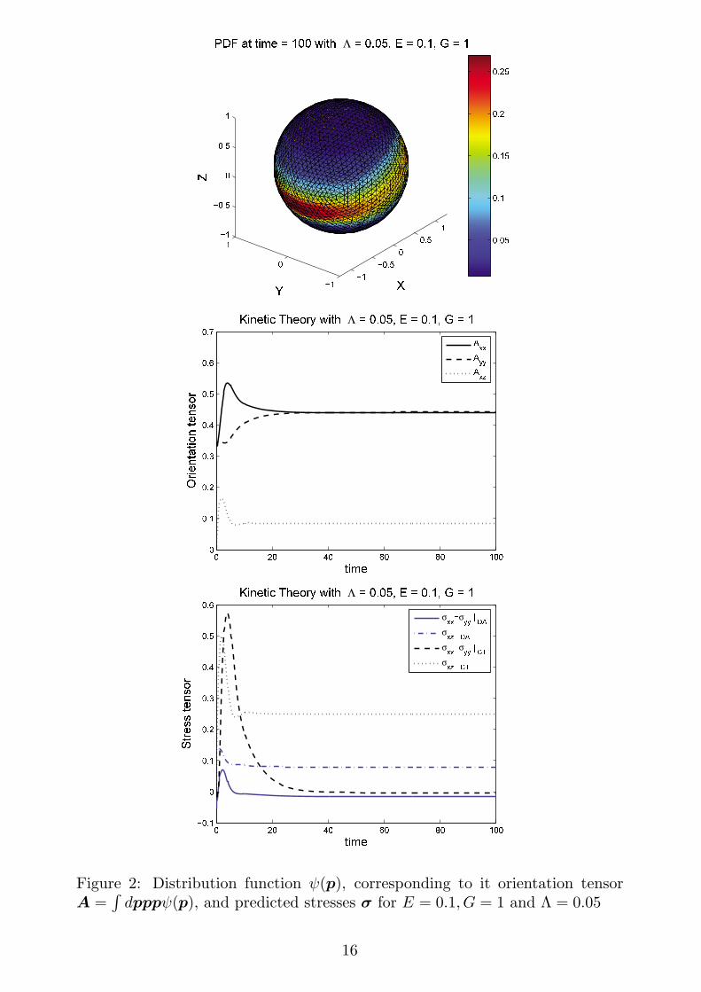
Figure 2: Distribution function �(�), corresponding to it orientation tensor� =
∫�����(�), and predicted stresses � for � = 0.1, � = 1 and Λ = 0.05
16

��
����
�
���
�
��
�
���
����
�
���
�
�
��� �� � ��� ��� Λ � ������ � � ���� � � �
�
�
���
���
���
���
���
���
���
� �� �� �� �� ����
���
���
���
���
���
���
���
�! �" #� $%& ��� Λ � ������ � � ���� � � �
��
'()*+,-,).+,*+/.(
011022013
� �� �� �� �� �������
��
����
�
���
�
���
�! �" #� $%& ��� Λ � ������ � � ���� � � �
��
4,(*//,*+/.(
σ11�σ22 5 67
σ13 5 67
σ11�σ22 5 89σ13 5 89
Figure 3: Distribution function �(�), corresponding to it orientation tensor� =
∫�����(�), and predicted stresses � for � = 0.1, � = 1 and Λ = 0.005
17

The smaller is the value of the parameters Λ the more important is the rolethe reversible part �(�, �) plays in the time evolution. In the solutions to themicrostructural equation presented on Figures 1, 2,3 this then manifests itselfin more intense elastic-type character of the responses. From the way we havederived in this section the thermodynamic formula �(�ℎ), we can anticipate thatthe difference between �(���ℎ��) and �(�ℎ) will be larger in the situations inwhich the advection (i.e. the term �(�, �)) plays in the time evolution playsa larger role (i.e. in the situation in which the suspension appears as a moreelastic fluid). This is indeed seen on the Figures 1,2,3.
3 Orientation tensor theory
In order to gain an additional insight into the relation between the microstruc-tural equation and the formula for the extra stress tensor, we shall repeat theanalysis made in Section 2 with another microstructural state variable �. Wechoose in this section � = �, where � is an orientation tensor. From the math-ematical point of view, � is a symmetric and positive definite matrix. From thephysical point of view, the orientation of the principal axis of the ellipsoid givenby the graph of < �, �� >= 1; � ∈ ℝ
3 and <,> denotes the inner product,represents the average orientation of the fibers and the thickness of the ellipsoidthe dispersion in the fiber distribution. In order to express the fact that thelength of fibers is fixed, we shall constrain � by ��� = 1. This constraint playsnow the same role as the constraint ∣�∣ = 1 that we used in kinetic theory inthe preceding section. For the sake of simplicity we shall limit ourselves in thissection to homogeneous suspensions, i.e. � is independent of the position vector�.
As an example of Eq.(3) with � = � we take the equation introduced recentlyin Wang et al. (2008). We shall call it WOT equation. The advection term �in this equation is particularly interesting. This makes then also the problemof the correct formula for the extra stress tensor particularly pertinent. Theadvection term in the WOT equation is given by
�(�,�) = Ω ⋅�−� ⋅Ω+ �� ⋅� + �� ⋅� − 2�[� + (1 − �)(�−� : �)] : �(33)
where � is the same parameter as in (5), � is a phenomenological scalar param-eter, and �, �, and � are certain functions (specified in Wang et al. (2008)) of�. The part � of Eq.(3) in the WOT equation is given by
�(�) = 2��� �̇(� − 3�) (34)
where �̇ =√
2� : �, � is the unit matrix, and �� > 0 is a phenomenologicalparameter. Regarding the dependence of �, �, and � on �, there are severalpossibilities to choose from.
In the particular case of the WOT equation corresponding to � = 1 and� = 1, the advection is passive. The the case � = 1 and � ∕= 1, corresponds to the
18

well known and often considered active advection. The new WOT advection cor-responds to � ∕= 1. The physics behind this new advection is the following. Theinfluence of the imposed flow on the orientation of the fibers is separated fromthe influence on the dispersity in the distribution. In terms of the orientationtensor, the separation into orientation and dispersity is made as follows. Thetensor � can always be represented as (�,�) where � = �⋅� ⋅�� ; �⋅�� = �,� is the unit matrix, ()� denotes the transpose, and � is a diagonal matrix. Ifwe see � as an ellipsoid (i.e. graph of < �, �� >= 1; � ∈ ℝ
3 and <,> denotesthe inner product) then � characterizes the rotation and � the shape of theellipsoid (i.e. a measure of the dispersion). Given an equation governing thetime evolution of �, a coupled system of equations governing the time evolutionof the two coordinates is implied. Wang et al. (2008) have suggested to modifythis system by modifying separately, and in a different way, equations governingthe time evolution of � and �.
We have now specified the state variables (1) as well as the microstructuralequation (3) and we can, following Section 2, proceed to the mechanical, ther-modynamical, and GENERIC investigations of the extra stress tensor. Beforedoing it we shall note that there is also another way to regard the orientationtensor �. The alternative to regarding � as a state variable with its own au-tonomous physical interpretation is to regard it as a reduction of the distributionfunction �(�), namely as ��� =
∫�� �����(�,�). Both the equation governing
the time evolution of � and the expressions for the extra stress tensor could bethen seen as reductions of the microstructural time evolution equations and ofthe expressions for the extra stress tensor discussed in Section 2. This is indeedan interesting avenue to follow but we shall not do it in this paper. Wang et al.
(2008) have derived (33) and (34) independently of kinetic equations governingthe time evolution of �(�). The only reference to the level of kinetic theory ap-pear in their analysis in the dependence of �, �, and � on �. These functionsarise in applying various closures (i.e. mappings � →֒ �(�)) identifying thesubmanifold of �(�) on which the kinetic level reduces to the level on which theorientation tensor serves as the state variable (see e.g. van Wieche-Booij (1971)distribution). In our discussion below, we shall simply consider �, �, and � asgiven functions of �. The only time where we shall need their specific form willbe in the numerical illustration. All the results regarding the formulas for theextra stress tensor will be obtained below with unspecified functions �, �, and�.
-
3.1 Mechanics
The formula that Wang et al. (2008) used to calculate the fiber contribution tothe extra stress tensor is the formula (9) in which � is not the fourth momentof the distribution function � as it in the context of the kinetic theory discussedin the preceding section but it is � appearing in (33).
19
3.2 Thermodynamics
We now completely follow Section 2.2. with the microstructural state variable� replaced by the orientation tensor �. The formula (14) takes in this contextthe form
�(�ℎ+)�� = −Φ���
∂���
∂(∂��
∂��
) (35)
With � given in (33), we obtain
�(�ℎ+)�� = �[Φ���
��� + Φ������ − 2Φ���
�����
−2(1 − �)Φ���(����� −����������)] (36)
Next, we turn to the specification of the free energy Φ. As in Section 2.2,
the free energy Φ(�,�) is a sum of the kinetic energy∫���
2
2� and a term that isindependent of � and that represents the contribution of the internal structure(i.e. the contribution of the fibers). The inequality (16) takes now the form
������ < 0 (37)
To identify the free energy, we proceed in the same way as in Section 2.2. Wenote that we can cast �(�) into the form
���(�) = −ΞΦ���(38)
for the dissipation potential
Ξ =1
2ΛΦ���
������(39)
and the free energy
Φ =
∫��
�2
2�+����
2(3��(�) − �� ���(�)), (40)
where
Λ =4����̇
����> 0 (41)
To verify the algebra involved we recall that ∂(���)∂���
= ��� and ∂(�� ����)∂���
= �−1�� ,
where �−1 denote the inverse of � and �−1�� are its elements.
From the physical point of view, the second term in (40) represents theentropy (first identified in Sarti and Marrucci (1973)), the first term guaranteesthe constraint ��� = �����. The equilibrium states (�,�)��, i.e. solutions of� = 0 and � = 0, are (�)�� = 0 and (���)�� = 1
3��� .The simplest dissipation potential (by definition a function of the derivative
of the free energy with respect to the state variable) satisfying the three prop-erties listed at the end of Section 2.2. is a positive definite quadratic functionof Φ�. The dissipation potential (19) in Section 2.2. has been chosen in thisway (in this example Φ� is, of course, replaced by Φ�). The dissipation func-tion (39) is again a positive definite quadratic function. Its positive definitnessfollows from (41) and the positive definitness of the orientation tensor �.
20

3.3 GENERIC
The advection represented by (33) is passive only for � = 1 and � = 1. Asin kinetic theory, the reversible part of the time evolution governed by (2),(3)is Hamiltonian only in this case. The Poisson bracket expressing this passiveadvection is given by (see Grmela (1988), Edwards et al. (2003) )
{�,�}(�,�) = {�,�}(�) +
∫��
[���
(∂����
∂�����
− ∂����
∂�����
)
+���
(����
∂���
∂��−����
∂���
∂��
)
+���
(����
∂���
∂��−����
∂���
∂��
)
−2������
(����
∂���
∂��−����
∂���
∂��
)](42)
It can easily be verified that �(�,�) implied by (20) and (42) is indeed (33)with � = 1 and � = 1.
Again, as in kinetic theory, the nonpassive advection (33) with � ∕= 1 and/or� ∕= 1 can be seen as an approximation of a time evolution taking place in anextended state space and involving both a passive advection and an irreversiblepart. In addition to the state variables (�,�), we adopt also �, having thephysical meaning of a conjugate to the gradient of the velocity disturbed by thepresence of fibers (see more in Gu and Grmela(2008)). The passive advectionof (�,�,�) is expressed in the Poisson bracket {�,�}�,�,�) = {�,�}(�,�) +{�,�}(�), where {�,�}(�,�) is given in (42) and {�,�}(�) is given by (seemore in Gu and Grmela (2008) )
{�,�}(�) = ���(����
����−����
����
)
+���(����
����−����
����
)
+���(����
����−����
����
)
+���(∂�(����
)���− ∂�(����
)���
)
+��� (����∂�(���
) −����∂�(���
))
+��� (����∂�(���
) −����∂�(���
))
+��� (����∂�(���
) −����∂�(���
))
−���(����
∂�(���) −����
∂�(���))
+���(∂�(����
)���− ∂�(����
)���
)(43)
The property {�,�} = −{�,�} is clearly visible in (43), the Jacobi identityfollows from the way the bracket (43) is derived in Gu and Grmela (2008).
By inserting {�,�}�,�,�) = {�,�}(�,�) + {�,�}(�) into (20) we obtainequations governing the time evolution of � and �. The former is
������
= ���(∂�(Φ��) + Φ���
) +���(∂�(Φ��) + Φ���
) (44)
21

If we add to the right hand side of that latter (see Gu and Grmela (2008) forits explicit form) an appropriate dissipation term that brings Φ� rapidly to the
stationary state for which����
= 0 and insert Φ� at the stationary state into(44) we arrive at � given in (33).
3.4 Comparison of different formulas for the extra stress
tensor
We have arrived at two formulas for the extra stress tensor. One, �(���ℎ��),given by (9), derived from mechanical arguments and the other, �(�ℎ), given by(36), derived from thermodynamic arguments or from the GENERIC structure.The formulas are different. All what we have said in Section 2.4 can now berepeated (except the arguments that uses the first equality in (28) since we donot have in this section any analog of the mechanical formula �(���ℎ�� ) thatis the same as the thermodynamic formula). Our conclusion is thus again thatthe thermodynamic formula is physically more justified than the mechanicalformula. An additional indirect argument supporting the expression (36) overthe expression (9) is that the parameters � and � quantifying the nonpassivityof the advection do not enter the formula (9) but do enter the formula (36).Details of the advection clearly influence the forces in the suspension and wecan therefore expect that the parameters appearing in the advection shouldshow up also in the formula for the extra stress tensor.
As in Section 2., we can suggest that the Dinh-Armstrong formula relates tothe thermodynamic formula by
�(���ℎ��)(�,�) ≈ �(�ℎ+)(�∣�̃�.(3)
) (45)
where �∣�̃�.(3)
) denotes a partial solution of Eq.(3). In this setting we are
however unable to identify �∣�̃�.(3)
) for which (45) would hold.
Now we comment about the particular choice (41) of the coefficient Λ madein Wang et al. (2008) (i.e. Λ ∼ �̇). While this choice is admissible if both statevariables (�,�) in Eqs.(2),(3) remain unconstrained (i.e. the setting used inthermodynamic and GENERIC arguments), it becomes inadmissible if � is seenas imposed from outside of the system. The former statement is true becausesolutions to Eqs.(2),(3) converge to the equilibrium state (i.e. to solutions ofΦ� = 0 and Φ� = 0) as �→ ∞. This then means that the stress converges tozero as � → ∞. If however the overall momentum of the fluid � is controlledfrom outside, the stress does not always approaches zero in the absence of flow.This happens in particular if the flow is suddenly stopped. In that case �̇ = 0,the term �(�) = 0, and the orientation of the fibers (i.e. �) ceases to evolvetowards equilibrium. Consequently, Φ� remains different from zero and thusalso the extra stress (36) remains different from zero. This is, of course, acontradiction since the stress tensor appearing in Eq.(2) can be different fromzero only in the presence of a flow.
How can be this contradiction (and thus a thermodynamics inadmissibilityof the choice (41) of the coefficient Λ) resolved?
22
The modification that will solve the problem is to replace �̇ in (41) (and thusin the last term on the right hand side of (33)) by (� + �̇), where � > 0 canbe arbitrarily small but different from zero. With this modification, Eqs.(2),(3),(33), (34), (41) become intrinsically compatible. In addition, the cessation ofthe imposed flow will be followed by relaxation of the fiber orientation and of thestress. We note that, in the case of lamellae replacing the fibers as suspendedparticles, a good agreement with results of experimental observations has beenachieved in Eslami et al. (2007) with a model that is essentially the same as(33) with �,�,� absent and Λ that does not involve �̇ at all.
Numerical illustration
Finally, we turn, as in Section 2, to a numerical illustration. Again, intentionis not to make a systematic numerical investigation of the differences in theimplied predicted stresses but to show, for a selected model parameters, thatthe predicted stresses are different but the difference is not large.
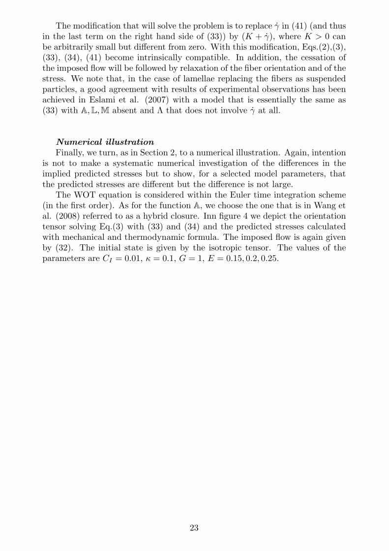
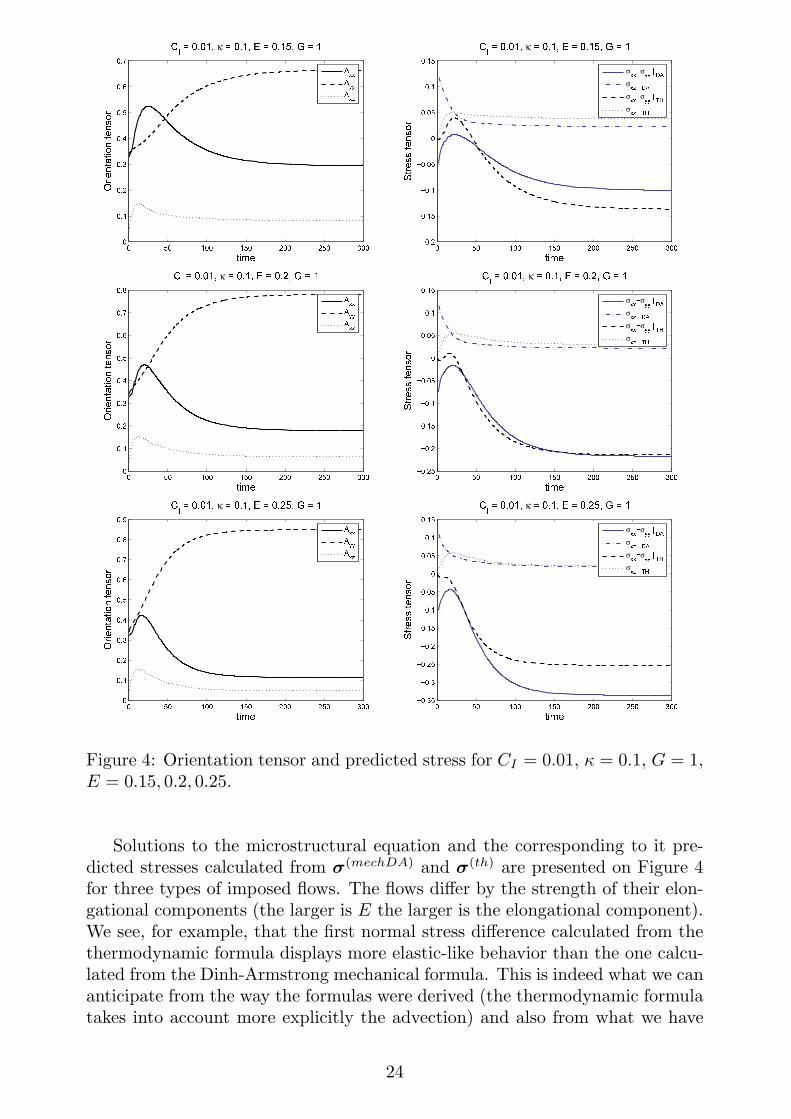
The WOT equation is considered within the Euler time integration scheme(in the first order). As for the function �, we choose the one that is in Wang etal. (2008) referred to as a hybrid closure. Inn figure 4 we depict the orientationtensor solving Eq.(3) with (33) and (34) and the predicted stresses calculatedwith mechanical and thermodynamic formula. The imposed flow is again givenby (32). The initial state is given by the isotropic tensor. The values of theparameters are �� = 0.01, � = 0.1, � = 1, � = 0.15, 0.2, 0.25.
23
� �� ��� ��� ��� ��� ����
���
���
���
���
���
���
���
� � ��� κ � � �� � � � ��� � � �
����
�����������������
!! "" !#
� �� ��� ��� ��� ��� ���$���
$����
$���
$����
�
����
���
����
� � ��� κ � � �� � � � ��� � � �
����
%�����������
σ!!$σ"" & '(
σ!# & '(σ!!$σ"" & )*σ!# & )*
� �� ��� ��� ��� ��� ����
���
���
���
���
���
���
���
��+
� � ��� κ � � �� � � � ,� � � �
����
�����������������
!! "" !#
� �� ��� ��� ��� ��� ���$����
$���
$����
$���
$����
�
����
���
����
� � ��� κ � � �� � � � ,� � � �
����
%�����������
σ!!$σ"" & '(
σ!# & '(σ!!$σ"" & )*σ!# & )*
� �� ��� ��� ��� ��� ����
���
���
���
���
���
���
���
��+
��-
� � ��� κ � � �� � � � ,�� � � �
����
�����������������
!! "" !#
� �� ��� ��� ��� ��� ���$����
$���
$����
$���
$����
$���
$����
�
����
���
����
� � ��� κ � � �� � � � ,�� � � �
����
%�����������
σ!!$σ"" & '(
σ!# & '(σ!!$σ"" & )*σ!# & )*
Figure 4: Orientation tensor and predicted stress for �� = 0.01, � = 0.1, � = 1,� = 0.15, 0.2, 0.25.
Solutions to the microstructural equation and the corresponding to it pre-dicted stresses calculated from �(���ℎ��) and �(�ℎ) are presented on Figure 4for three types of imposed flows. The flows differ by the strength of their elon-gational components (the larger is � the larger is the elongational component).We see, for example, that the first normal stress difference calculated from thethermodynamic formula displays more elastic-like behavior than the one calcu-lated from the Dinh-Armstrong mechanical formula. This is indeed what we cananticipate from the way the formulas were derived (the thermodynamic formulatakes into account more explicitly the advection) and also from what we have
24

seen on Figures 1,2,3 in the setting of kinetic theory.
4 Concluding remarks
The complex fluid under consideration in this paper is a suspension of fibers.The distribution function �(�,�) and the orientation tensor � have been cho-sen as microstructural state variables. We have followed two routes leading toformulas expressing the stress tensor as a function of the microstructural statevariables: 1. mechanical and 2. thermodynamical.
1. Mechanics
This is the most common and most frequently used approach to calculatestresses. The physics on which this approach is based is the interpretation ofthe equation governing the time evolution equation of the fluid velocity as acontinuum version of Newton’s law. The stress tensor is then calculated byidentifying the local surface forces acting on the microstructure. The directnessof the relation between what is calculated and what is measured that is inher-ent to this method is certainly the main reason for its popularity. The mainproblem that we see in the mechanical approach is that the microstuctural timeevolution equation on the one hand and the formula for the extra stress tensoron the other hand arise in two parallel and largely independent of each otherconsiderations. Their compatibility is thus in question. The intrinsic compati-bility of the microstructural dynamics and macroscopic stresses does not comenaturally in the mechanical approach and is never completely guaranteed.
2. Thermodynamics
The thermodynamic approach is based on the requirement that solutions tothe equations governing the time evolution of the overall fluid velocity and themicrostructure agree with one particular experimental observation. The obser-vation is that externally unforced suspensions reach states, called equilibriumstates, at which their behavior is well described by classical thermodynamics.The formula for the stress tensor arises as a compatibility condition relatingthe microstructural and the overall velocity equations. The physics entering theanalysis of the microstructural dynamics and the physics entering the analysisof the extra stress tensor is thus guaranteed to be identical. The disadvantageof the thermodynamic approach is that the the formula for the extra stress ten-sor is derived for externally unforced systems and is used then in rheologicalinvestigations of driven systems.
We have also explored a stronger version (called GENERIC) of the thermo-dynamic approach. In addition to the requirement of the agreement of solutionsto the governing equations with the experimental observations constituting thebasis of equilibrium thermodynamics, GENERIC requires that the reversibleparts of the time evolution of the velocity and the microstructure represent to-gether a Hamiltonian time evolution for which the free energy is a constant ofmotion. We have shown that the GENERIC approach leads to the same for-mulas for the extra stress tensor as the thermodynamic approach that does notuse the Hamiltonian structure. Moreover, we have noted that the Hamiltonian
25
structure, that is present only when the microstructure is passively advected,can be recovered also in the case of a physically more realistic nonpassive ad-vection. What is needed is an extended setting in which the microstructuralstate variables involve an additional velocity type variable (as e.g. the angu-lar momentum of the fibers). The nonpassive advection is manifested in suchextended setting in the dissipation of the added velocity type state variable, inparticular then with its coupling with the dissipation of the fluid velocity.
Results for fiber suspensions and two choices of microstructural
state variables.
Given a microstructural equation there are, in general, infinitely many corre-sponding to it formulas for the extra stress tensor that look very differently butare equivalent in the sense that they all imply the same predicted stresses. Bya predicted stress we mean the stress obtained by evaluating the expression forthe stress tensor at solutions to the microstructural equation. Predicted stressesare the stresses measured in rheological observations. The reason why there are,in general, infinitely many equivalent formulas for the extra stress tensor is thatthere are, in general, infinitely many partial solutions to the microstructuralequation. Let us see the process of getting solution to the microstructural equa-tion as a gradual process in which the space in which the solutions are searchedis being gradually restricted. Partial solutions are, in our terminology, the mi-crostructural state variables restricted to such submanifolds. From the physicalpoint of view, the gradual process of restrictions leading to partial solutionscan be interpreted as the process of a descend to more macroscopic (i.e. lessdetailed) levels of description. The submanifolds are also called closures (seemore in Section 2.4 and in Grmela (2010)).
In this paper we have seen that the mechanical and the thermodynamic ap-proaches lead to identical formulas for the extra stress tensor only in kinetictheory, i.e. with the distribution function � playing the role of microstructuralstate variable, and only with the mechanical formula derived in Chan and Teren-tjev (2007). The Dinh-Armstrong mechanical formula, that can be applied alsofor the orientation tensor � playing the role of microstructural state variable, isdifferent from the formula arising in thermodynamics. Is this formula equivalent(in the sense of the previous paragraph) to the thermodynamic formula? In thecontext of the kinetic theory we identify a restricted distribution function that,if inserted into the thermodynamic formula, makes it look similar to the Dinh-Armstrong mechanical formula. The identified restricted distribution functionis however only an approximative solution (valid for small velocity gradients ofthe imposed flow) to the kinetic equation. The absence in the Dinh-Armstrongformula of details of the advection of the microstructure is an indication of thenon-equivalence of the Dinh-Armstrong and the thermodynamic formulas. Thedifference is also seen in numerical illustrations developed in both the kinetictheory and the orientation tensor theory. In general, we see that the larger isthe role of the time reversible part of the time evolution of the microstructure(i.e. the role of the advection) the larger is the difference in predicted stresses.
26

Acknowledgement
One of the authors, M.G., would like to thank Natural Sciences and Engi-neering Research Council of Canada for financial support and Charles Tuckerfor stimulating discussion and for suggestions to improve the presentation ofthis paper.
References
Arnold, V.I., ”Sur la geometrie differentielle des groupes de Lie de dimensioninfini et ses applications a l’hydrodynamique des fluides parfaits”, Ann. Inst.Fourier 16, 319-361 (1966)
Batchelor, G.K., ”The stress system in suspensions of force-free particles”,J. Fluid Mech. 41, 545 (1970)
Batchelor, G.K., ”The stress generated in a non-dilute suspension of elon-gated particles by pure straining motion”, J. Fluid Mech. 46, 593 (1971)
Beris, A.N.and Edwards, B.J., ”Thermodynamics of flowing systems”, Ox-ford Univ. Press, Oxford (1994)
Chan, C.J. and Terentjev, E.M., ”Non-equilibrium statistical mechanics ofliquid crystals: relaxation, viscosity and elasticity”, J. Phys. A: Math. Theor.40, R103 (2007)
Clebsch, A., ”Ueber die Integration der hydrodynamische Gleichungen”, J.Reine Angew. Math, 56 1-10 (1895)
Dinh, S. M., and R. C. Armstrong, A rheological equation of state for semi-concentrated fiber suspensions, J. Rheol. 28, 207227 (1984).
Doi, M. ”Variational principle for the Kirkwood theory for the dynamics ofpolymer solutions and suspensions”, J. Chem. Phys. 79, 5080 (1983)
Dzyaloshinskii, I.E., Volovick, G.E., ”Poisson brackets in condense matterphysics”, Ann. Phys. (NY) 125, 67-97 (1980)
Edwards, B.J., Dressler, M., Grmela, M., Ait-Kadi A., ”Rheological modelswith microstructural constraints”, Rheol. Acta 42, 64-72 (2003)
Eslami, H. Grmela, M. Bousmina, M. ”A mesoscopic rheological model ofpolymer/layered silicate nanocomposites”, J. Rheol. 51, 1189-1222 (2007)
Evans, J.G., Ph.D Dissertation, Cambridge University (1975)Feng, J., Sgalari, G., Leal, L.G., ”A theory for flowing polymers with orien-
tational distribution”, J. Rheol. 44, 1085 (2000)Grmela, M., ”Particle and Bracket Formulations of Kinetic Equations”, Con-
temporary Math. 28, 125-132 (1984), Physics Letters A 102, 355 (1984)Grmela, M., ”Stress tensor in generalized hydrodynamics”, Phys.Letters A,
111A, 41-44 (1985)Grmela, M., ”Hamiltonian dynamics of incompressible elastic fluids”, Phys.
Lett. A 130, 81-86 (1988)
27

Grmela M.and Ottinger, H.C., ”Dynamics and Thermodynamics of ComplexFluids:General Formulation”, Phys.Rev.E 56, 6620-6633 (1997)
Grmela, M., Lafleur, P.G., ”Kinetic theory and hydrodynamics of rigid bodyfluids” J. Chem. Phys. 100, 6956-6972 (1998)
Grmela,M. ”Complex fluids subjected to external influences”, J. Non-NewtonianFluid Mech. 96, 221-254 (2001)
Grmela, M. ”Reciprocity relations in thermodynamics”, Physica A 309. 304-328 (2002)
Grmela, M. ”Geometry of mesoscopic dynamics and thermodynamics”, J.Non-Newtonian Fluid Mech. 120, 137-147 (2004)
Grmela, M. ”Stress tensor in fiber suspensions”, Phys.Lett.A, 372, 4267-4270 (2008)
Grmela, M. ”Multiscale equilibrium and nonequilibrium thermodynamicsin chemical engineering”, Advances in Chemical Engineering, Vol.39, 75-128(2010) edited by D.H. West and G. Yablonsky, Elsevier Inc.
Gu, J.F. and Grmela, M. ”GENERIC model of active advection”, J. Non-Newtonian Fluid Mech. 152, 12-26 (2008)
Kaufman, A.N. ”Dissipative Hamiltonian systems: A unifying principle”,Phys. Letters A 100, 419 (1984)
Lipscomb, G. G., M. M. Denn, D. U. Hur, and D. V. Boger, The flow of fibersuspensions in complex geometries, J. Non-Newtonian Fluid Mech. 26, 297325(1988)
Marsden, J.E., Ratiu, T.S. ”Introduction to Mechanics and Symmetry”,Texts in Applied mathematics,. Volume 17, Springer, New York, ((1999)
Morrison, P.J., Bracket formulation for irreversible classical fields, Phys.Letters A 100, 423 (1984)
Ottinger, H.C. ”General projection operator formalism for the dynamics andthermodynamics of complex fluids”, Phys. Rev. E 47, 1416 (1998)
Ottinger, H.C. ”Beyond equilibrium thermodynamics”, Wiley (2005)Ottinger, H.C. and Grmela, M. ”Dynamics and Thermodynamics of Com-
plex Fluids: Illustration of the General Formalism”, Phys.Rev.E 56, 6633-6650(1997)
Sarti, G.C., G. Marrucci, ”Thermomechanics of dilute polymer solutions:multiple bead-spring model”, Chem.Eng.Sci. 28, 1053 (1973) (1973)
Sircar, S., Wang, Q., ”Dynamics and rheology of biaxial liqud crystal poly-mers in shear flows” J. Rheol. 53, 819 (2009)
van Wiechen, P.H., Booij, H.C., J. Eng. Math. ” A General Solution to theNecklace Model Problem in the Rheology of macromolecules” 5, 89-98 (1971)
Wang,J., J.F. O’Gara, C.L. Tucker III, ”An objective model for slow orien-tation kinetics in concentrated fiber suspensions: Theory and rheological evi-dence”, J.Rheol. 52 1179-1200 (2008)
Wang, Q. ”A hydrodynamic theory for solutions of nonhomogeneous nematicliquid crystalline polymers of different configurations”, J. Chem. Phys. 116,9120 (2002)
28