Exterminating the dynamic change bug: A concrete … · Exterminating the Dynamic Change Bug 299 in...

Information Systems Frontiers 3:3, 297–317, 2001C© 2001 Kluwer Academic Publishers. Manufactured in The Netherlands.

Exterminating the Dynamic Change Bug: A ConcreteApproach to Support Workflow Change

W.M.P. van der AalstEindhoven University of Technology, Faculty of Technologyand Management, Department of Information and Technology,P.O. Box 513, NL-5600 MB, Eindhoven, The NetherlandsE-mail: [email protected]

Abstract. Adaptability has become one of the major researchtopics in the area of workflow management. Today’s workflowmanagement systems have problems dealing with both ad-hocchanges and evolutionary changes. As a result, the workflowmanagement system is not used to support dynamically chang-ing workflow processes or the workflow process is supported ina rigid manner, i.e., changes are not allowed or handled outsideof the workflow management system. In this paper, we focus on anotorious problem caused by workflow change: the “dynamicchange bug” (Ellis et al., Proceedings of the Conference onOrganizational Computing Systems, Milpitas, California, ACMSIGOIS, ACM Press, New York, 1995, pp. 10−21). The dy-namic change bug refers to errors introduced by migrating acase (i.e., a process instance) from the old process definition tothe new one. A transfer from the old process to the new processcan lead to duplication of work, skipping of tasks, deadlocks,and livelocks. This paper describes an approach for calculatinga safe change region. If a case is in such a change region, thetransfer is postponed.

Key Words. workflow management, workflow change, dynamicchange, petri nets

1. Introduction

Workflow management technology aims at the auto-mated support and coordination of business processesto reduce costs and flow times, and increase quality ofservice and productivity. A critical challenge for work-flow management systems is their ability to respondeffectively to changes. Changes may range from ad-hoc modifications of the process for a single customerto a complete restructuring of the workflow processto improve efficiency. Today’s workflow managementsystems are ill suited to dealing with change. They

typically support a more or less idealized version of thepreferred process. However, the real run-time processis often much more variable than the process specifiedat design-time. The only way to handle changes is to gobehind the system’s back. If users are forced to bypassthe workflow management system quite frequently, thesystem is more a liability than an asset. Therefore, wetake up the challenge to find techniques to add flexi-bility without loosing the support provided by today’ssystems.

Typically, there are two types of changes: (1) ad-hocchanges and (2) evolutionary changes. Ad-hoc changesare handled on a case-by-case basis. In order to providecustomer specific solutions or to handle rare events,the process is adapted for a single case or a limitedgroup of cases. Evolutionary change is often the re-sult of reengineering efforts. The process is changedto improve responsiveness to the customer or to im-prove the efficiency (do more with less). The trendis towards an increasingly dynamic situation whereboth ad-hoc and evolutionary changes are needed toimprove customer service and reduce costs. In this pa-per, we restrict ourselves to evolutionary change. Infact, ad-hoc change is partially handled by at leasttwo existing workflow management systems: InCon-cert (Tibco/InConcert) and Ensemble (FileNet).

The term dynamic change refers to the problemof handling old cases in a new process, e.g., how totransfer cases to a new version of the process. The dy-namic change problem which was first mentioned byEllis, Keddara, and Rozenberg in 1995 (Ellis et al.,1995). To discuss this problem we use the two Petrinets shown in Fig. 1. For an introduction to Petri nets(Reisig and Rozenberg, 1998) we refer to Appendix A.If the sequential workflow process (left) is changed

297

298 van der Aalst

Fig. 1. The dynamic change bug.

into the workflow process where tasks send goods andsend bill can be executed in parallel (right) there areno problems, i.e., it is always possible to transfer a casefrom the left to the right. The sequential process has fivepossible states and each of these states corresponds toa state in the parallel process. For example, the statewith a token in s3 is mapped onto the state with a to-ken in p3 and p4. In both cases, tasks prepare shipmentand send goods have been executed and send bill andrecord shipment still need to be executed. Now con-sider the situation where the parallel process is changedinto the sequential one, i.e., a case is moved from theright-hand-side process to the left-hand-side process.For most of the states of the right-hand-side processthis is no problem, e.g., a token in p1 is moved to s1, atoken in p3 and a token in p4 are mapped onto one tokenin s3, and a token in p4 and a token in p5 are mappedonto one token in s4. However, the state with a token inboth p2 and p5 (prepare shipment and send bill havebeen executed) causes problems because there is nocorresponding state in the sequential process (it is notpossible to execute send bill before send goods). If thecase is moved to place s2 or place s3, task send billis executed twice. If the case is moved to place s4 orplace s3, task send goods is not executed at all. Theexample in Fig. 1 shows that it is not straightforwardto migrate old cases to the new process after a change.

The problem illustrated in Fig. 1 is a result of re-ducing the degree of parallelism by making the processsequential. Similar problems occur when the order oftasks is changed, e.g., two sequential tasks are swapped.Extending the workflow with new tasks, removingparts, or aggregating a group of tasks into a single taskmay result in similar problems. When changing theworkflow on-the-fly, i.e., running cases are transferredto the new process definition, the dynamic change bugis likely to occur. Therefore, the problem is very rele-vant for a workflow management system truly support-ing adaptive workflow. Today’s workflow managementsystems are not able to handle this problem. These sys-tems use a versioning mechanism, i.e., every changeleads to a new version and each case refers to the ap-propriate version. If a case starts using a version ofthe process, it will continue to use this version. Theversioning mechanism may be suitable in some situa-tions. An administrative process with a short flow timeis a good candidate for a versioning mechanism. How-ever, there are many situations where the mechanismis not appropriate. If a case has a long flow time, thenit is often not acceptable to handle existing cases thisway. Consider for example a process for handling mort-gage loans. Mortgages typically have a duration of 20to 30 years. If the process changes every month, thiswould lead to hundreds of different versions running

Exterminating the Dynamic Change Bug 299

in parallel. To reduce cost and to keep the processesmanageable, the number of active versions (i.e., ver-sions still used by cases) should be kept to a minimum.Also for processes with a shorter flow time, it may beundesirable to have many versions running in paral-lel. In fact, there may be legal reasons (e.g., startingfrom January 2001 a new step in the process is manda-tory), forcing the transfer of cases to the new process.Unfortunately, problems such as the one illustrated byFig. 1 make a direct transfer hazardous. Without exter-minating the dynamic change bug the next generationof workflow management systems will be unable totruly support adaptive workflow.

To exterminate the dynamic change bug, we proposean approach that automatically calculates the changeregion. The change region is determined by comparingthe old and the new process and extending the regionsthat have changed with regions that are affected bythe change. Due to the possibly complex mixture ofdifferent routing constructs (choice, synchronization,iteration, etc.), it is far from trivial to compute the re-gions that are affected. If a case is in the change region,it cannot be transferred. The transfer is delayed untilthe change region is empty. We will show that postpon-ing the migration of a case until the change region isempty, results in the correct execution of the case. Fora short period (depending on the change region), thereare multiple versions but as soon as a transfer is safe thecase is handled according to the new process definition.

The approach differs from existing approaches(Aalst and Basten, 2001; Aalst, Desel and Oberweis,2000b; Aalst et al., 2000a; Casati et al., 1998; Reichertand Dadam, 1998; Ellis, Keddara, and Rozenberg,1995; Ellis and Keddara, 2000a, 2000b; Michelis andEllis, 1998; Keddara, 1999; Joeris and Herzog, 1998;Agostini and Michelis, 2000; Sadiq, Marjanovic andOrlowska, 2000; Vossen and Weske, 1999; Weske,2000) in the sense that no local transformation rulesare assumed and that the calculation of the change re-gion is based on the structure of the workflow graph.Note that we restrict ourselves to logical errors in thecontrol-flow resulting from change. Clearly, there areother types of constraint violations. Moreover, changecan also result in resource or data conflicts. These prob-lems are outside the scope of this paper.

The remainder of this paper is organized as fol-lows. First, we introduce the basic concepts and thetechniques we are going to use. The approach pre-sented in this paper is based on a special subclassof Petri nets (WF-nets) and a notion of correctness

named soundness (Aalst, 1998b, 2000). In Section 3,we clearly define to problem (the dynamic change bug)and give a number of dynamic change examples. Then,we present the algorithm to calculate the change region.In Section 5, we compare this approach with other ap-proaches addressing the dynamic change problem. Fi-nally, we summarize the results presented and concludewith our future plans.

2. Preliminaries

This section introduces the basic concepts, definitions,and techniques used to tackle the dynamic changebug. For a more elaborate discussion on these top-ics, we refer to Aalst (1998b, 2000), Ellis, Keddaraand Rozenberg (1995), and Ellis and Nutt (1993).For an introduction to Petri nets we refer to Deseland Esparza (1995), Murata (1989), and Reisig andRozenberg (1998) and the appendix.

2.1. Workflow process definitionsThe term workflow management (Koulopoulos, 1995;Lawrence, 1997; Jablonski and Bussler, 1996) refers tothe domain which focuses on the logistics of businessprocesses. There are also people who use the term officelogistics. The ultimate goal of workflow managementis to make sure that the proper activities are executed bythe right person at the right time. Although it is possibleto do workflow management without using a workflowmanagement system, most people associate workflowmanagement with workflow management systems. Theworkflow Management Coalition (WfMC) defines aworkflow management system as follows (WFMC,1996): A system that completely defines, manages,and executes workflows through the execution of soft-ware whose order of execution is driven by a com-puter representation of the workflow logic. Otherterms to characterize a workflow management systemare: ‘business operating system’, ‘workflow manager’,‘case manager’ and ‘logistic control system’.

Workflows are case-based, i.e., every piece of workis executed for a specific case. Examples of cases area mortgage, an insurance claim, a tax declaration, anorder, or a request for information. Cases are often gen-erated by an external customer. However, it is also pos-sible that a case is generated by another departmentwithin the same organization (internal customer). Thegoal of workflow management is to handle cases as

300 van der Aalst

efficiently and effectively as possible. A workflow pro-cess is designed to handle similar cases. Cases are han-dled by executing tasks in a specific order. The work-flow process definition specifies which tasks need tobe executed and in what order. Alternative terms forworkflow process definition are: ‘procedure’, ‘flow di-agram’ and ‘routing definition’. Since tasks are exe-cuted in a specific order, it is useful to identify con-ditions which correspond to causal dependencies be-tween tasks. A condition holds or does not hold (trueor false). Each task has pre- and postconditions: thepreconditions should hold before the task is executed,and the postconditions should hold after execution ofthe task. Many cases can be handled by following thesame workflow process definition. As a result, the sametask has to be executed for many cases. A task thatneeds to be executed for a specific case is called a workitem. An example of a work item is: execute task ‘sendrefund form to customer’ for case ‘complaint sent bycustomer Baker’. Most work items are executed by aresource. A resource is either a machine (e.g., a printeror a fax) or a person (participant, worker, employee).To facilitate the allocation of work items to resources,resources are grouped into classes. A resource class isa group of resources with similar characteristics. Theremay be many resources in the same class and a resourcemay be a member of multiple resource classes. If a re-source class is based on the capabilities (i.e., functionalrequirements) of its members, it is called a role. If theclassification is based on the structure of the organiza-tion, such a resource class is called an organizationalunit. A work item which is being executed by a specificresource is called an activity.

Of all workflow perspectives (e.g., control-flow,data, organization, task, operation) (Jablonski andBussler, 1996), the control-flow perspective is the mostprominent one, because the core of any workflow sys-tem is formed by the processes it supports. In thecontrol-flow dimension building blocks such as theAND-split, AND-join, OR-split, and OR-join are usedto model sequential, conditional, parallel and iterativerouting (WFMC, 1996). Clearly, a Petri net can be usedto specify the routing of cases. See Appendix A for anintroduction to Petri nets. Tasks are modeled by transi-tions and causal dependencies are modeled by placesand arcs. In fact, a place corresponds to a conditionwhich can be used as pre- and/or post-condition fortasks. An AND-split corresponds to a transition withtwo or more output places, and an AND-join corre-sponds to a transition with two or more input places.

OR-splits/OR-joins correspond to places with multipleoutgoing/ingoing arcs. Moreover, in Aalst (1998a) it isshown that the Petri net approach also allows for usefulrouting constructs absent in many workflow manage-ment systems.

A Petri net which models the control-flow dimen-sion of a Workflow, is called a WorkFlow net (WF-net).It should be noted that a WF-net specifies the dynamicbehavior of a single case in isolation.

Definition 1 (WF-net). A Petri net PN = (P, T, F)is a WF-net (WorkFlow net) if and only if:

(i) There is one source place i ∈ P such that •i = ∅.(ii) There is one sink place o ∈ P such that o• = ∅.

(iii) Every node x ∈ P ∪ T is on a path from i to o.

A WF-net has one input place (i) and one output place(o) because any case handled by the procedure rep-resented by the WF-net is created when it enters theworkflow management system and is deleted once it iscompletely handled by the workflow management sys-tem, i.e., the WF-net specifies the life-cycle of a case.The third requirement in Definition 1 has been added toavoid ‘dangling tasks and/or conditions’, i.e., tasks andconditions which do not contribute to the processingof cases. If there is no confusion possible we will usei and o to denote the input place and output place ofa WF-net. If confusion is possible, we add a subscriptreferring to the proper WF-net, i.e., iPN and oPN denotethe input place and output place of the WF-net P N .

Given the definition of a WF-net it is easy derive thefollowing properties.

Proposition 1 (Properties of WF-nets). Let PN =(P, T, F) be Petri net.

– If PN is WF-net with source place i, then for anyplace p ∈ P: •p = ∅ or p = i, i.e., i is the onlysource place.

– If PN is WF-net with sink place o, then for anyplace p ∈ P: p• = ∅ or p = o, i.e., o is the onlysink place.

– If PN is a WF-net and we add a transition t∗ toPN which connects sink place o with source placei (i.e., •t∗ = {o} and t∗• = {i}), then the resultingPetri net is strongly connected.

– If PN has a source place i and a sink place o andadding a transition t∗ which connects sink place owith source place i yields a strongly connected net,then every node x ∈ P ∪ T is on a path from i to oin PN and PN is a WF-net.


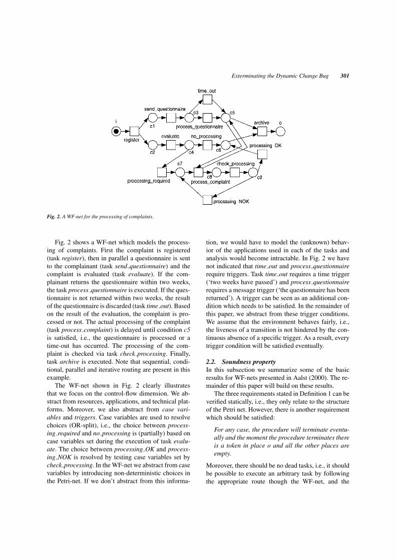
Fig. 2. A WF-net for the processing of complaints.

Fig. 2 shows a WF-net which models the process-ing of complaints. First the complaint is registered(task register), then in parallel a questionnaire is sentto the complainant (task send questionnaire) and thecomplaint is evaluated (task evaluate). If the com-plainant returns the questionnaire within two weeks,the task process questionnaire is executed. If the ques-tionnaire is not returned within two weeks, the resultof the questionnaire is discarded (task time out). Basedon the result of the evaluation, the complaint is pro-cessed or not. The actual processing of the complaint(task process complaint) is delayed until condition c5is satisfied, i.e., the questionnaire is processed or atime-out has occurred. The processing of the com-plaint is checked via task check processing. Finally,task archive is executed. Note that sequential, condi-tional, parallel and iterative routing are present in thisexample.

The WF-net shown in Fig. 2 clearly illustratesthat we focus on the control-flow dimension. We ab-stract from resources, applications, and technical plat-forms. Moreover, we also abstract from case vari-ables and triggers. Case variables are used to resolvechoices (OR-split), i.e., the choice between process-ing required and no processing is (partially) based oncase variables set during the execution of task evalu-ate. The choice between processing OK and process-ing NOK is resolved by testing case variables set bycheck processing. In the WF-net we abstract from casevariables by introducing non-deterministic choices inthe Petri-net. If we don’t abstract from this informa-

tion, we would have to model the (unknown) behav-ior of the applications used in each of the tasks andanalysis would become intractable. In Fig. 2 we havenot indicated that time out and process questionnairerequire triggers. Task time out requires a time trigger(‘two weeks have passed’) and process questionnairerequires a message trigger (‘the questionnaire has beenreturned’). A trigger can be seen as an additional con-dition which needs to be satisfied. In the remainder ofthis paper, we abstract from these trigger conditions.We assume that the environment behaves fairly, i.e.,the liveness of a transition is not hindered by the con-tinuous absence of a specific trigger. As a result, everytrigger condition will be satisfied eventually.

2.2. Soundness propertyIn this subsection we summarize some of the basicresults for WF-nets presented in Aalst (2000). The re-mainder of this paper will build on these results.

The three requirements stated in Definition 1 can beverified statically, i.e., they only relate to the structureof the Petri net. However, there is another requirementwhich should be satisfied:

For any case, the procedure will terminate eventu-ally and the moment the procedure terminates thereis a token in place o and all the other places areempty.

Moreover, there should be no dead tasks, i.e., it shouldbe possible to execute an arbitrary task by followingthe appropriate route though the WF-net, and the

302 van der Aalst

WF-net should be safe. These additional requirementsfor WF-nets correspond to the so-called soundnessproperty.

Definition 2 (Sound). A procedure modeled by aWF-net PN = (P, T, F) is sound if and only if:

(i) For every state M reachable from state i , thereexists a firing sequence leading from state M tostate o. Formally:1

∀M (i∗→ M) ⇒ (M

∗→ o)

(ii) State o is the only state reachable from state i withat least one token in place o. Formally:

∀M (i∗→ M ∧ M ≥ o) ⇒ (M = o)

(iii) There are no dead transitions in (PN , i). Formally:

∀t∈T ∃M,M ′ i∗→ M

t→ M ′

(iv) (PN , i) is safe.

Note that the soundness property relates to the dynam-ics of a WF-net. The first requirement in Definition 2states that starting from the initial state (state i), it is al-ways possible to reach the state with one token in placeo (state o). If we assume a strong notion of fairness, thenthe first requirement implies that eventually state o isreached. Strong fairness means that in every infinitefiring sequence, each transition fires infinitely often.The fairness assumption is reasonable in the context of

Fig. 3. Another WF-net for the processing of complaints.

workflow management: All choices are made (implic-itly or explicitly) by applications, humans or externalactors. Clearly, they should not introduce an infiniteloop. Note that the traditional notions of fairness (i.e.,weaker forms of fairness with just local conditions, e.g.,if a transition is enabled infinitely often, it will fire even-tually) are not sufficient. See Aalst (1998b) and Kindlerand Aalst (1999) for more details. The second require-ment states that the moment a token is put in place o,all the other places should be empty. Sometimes theterm proper termination is used to describe the firsttwo requirements (Gostellow et al., 1972). The thirdrequirement states that there are no dead transitions(tasks) in the initial state i. The last requirement statesthat the WF-net should be safe, i.e., for a single casein isolation, it is not allowed to have multiple tokens inone place.

Fig. 2 is an example of a WF-net which is sound.Fig. 3 shows a WF-net which is not sound. This WF-net is an attempt to simplify the one shown in Fig. 2:The token in c5 is now actually removed by pro-cess complaint, i.e., process complaint does not returnthe token and, therefore, archive no longer needs to re-move the remaining token in c5. Although this mayseem to be a good idea, there are several deficien-cies. First of all, tasks may be executed after comple-tion, e.g., after firing register, evaluate, no processing,and archive there is a token in place o indicatingcompletion, but at the same time send questionnaireis enabled. Second, there is a potential deadlock: If


processing NOK fires, then the WF-net gets stuck inthe state with just a token in c7. Any attempt to ex-ecute task processing complaint multiple times willlead to a deadlock situation. Clearly, the WF-net is notsound.

Given a WF-net PN = (P, T, F), we want todecide whether PN is sound. In (Aalst, 2000) we haveshown that soundness corresponds to liveness andboundedness. To link soundness to liveness and bound-edness, we define an extended net PN = (P, T , F).PN is the Petri net obtained by adding an extratransition t∗ which connects o and i . The extendedPetri net PN = (P, T , F) is defined as follows:P = P , T = T ∪ {t∗}, and F = F ∪ {〈o, t∗〉, 〈t∗, i〉}.In the remainder, we will call such an extended netthe short-circuited net of PN . The short-circuitednet allows for the formulation of the following theorem.

Theorem 1. A WF-net PN is sound if and only if(PN , i) is live and safe.

Proof: See (Aalst, 2000) �

This theorem shows that standard Petri-net-based anal-ysis techniques can be used to verify soundness. Theshort-circuited version of the WF-net shown in Fig. 2 islive and safe. The short-circuited version of the WF-netshown Fig. 3 is not live and not safe.

3. Dynamic Change: The Problem

Today’s workflow management systems typically sup-port two types of change. The systems aiming at pre-defined and well-structured workflow processes, oftenreferred to as production workflow, support a version-ing mechanism (cf. Section 1). Most of the availablesystems fit into this category (e.g., Staffware, MQ Se-ries workflow, and COSA). Only a few systems supporta different form of change by binding private processdefinitions to cases. The latter class of workflow sys-tems support ad-hoc workflow and examples of suchsystems are InConcert (InConcert/TIBCO) and Ensem-ble (Filenet).

The versioning mechanism supported by most ofthe systems binds each case to a specific version of theworkflow. A version itself will never change: Only newversions can be added. Therefore, each case will fol-low the procedure defined in the corresponding versionand will not be influenced by changes during its life-time. Only new cases benefit from change and typically

follow the most recent version of the workflow at themoment of creation.

Systems supporting ad-hoc workflow associate aworkflow process definition with each case, i.e., eachworkflow instance carries its own description. Thesesystems typically allow for limited change, e.g., in In-Concert it is possible to remove and/or add tasks in partsof the process which still need to be executed. Clearly,these systems do not support evolutionary changes asdescribed in the introduction.

Both types of change (versioning mechanism andad-hoc workflow) are quite easy to implement and arenot confronted with problems such as the one illus-trated by Fig. 1. The dynamic change problem, whichwas first mentioned by Ellis, Keddara, and Rozenbergin 1995 (Ellis et al., 1995) is not addressed at all bythese systems. Nevertheless, there is a clear need formechanisms which allow for the migration of instances(cases) from one process definition to another. Thereare many examples of workflow processes with a con-siderable number of instances which have a long flowtime. Consider for example mortgage loans which havea life-cycle of decades. In such situations the versionmechanism is not acceptable: Too many versions wouldbe active thus resulting in an unmanageable workflow.There may also be legal and economical reasons for themigration of instances (cases) from one process defini-tion to another. If the law changes, some processes maybe affected and the organization may be forced to mi-grate cases, i.e., to handle existing cases the new way.The solution provided by ad-hoc workflow systems isoften not acceptable, because every instance needs tobe modified by hand and there is no control over theuniformity of the workflow process. Moreover, the so-lutions provided by systems like InConcert restrict themodeling language to avoid problems such as the oneillustrated by Fig. 1 (e.g., no iteration). Therefore, wetackle the dynamic change problem using the conceptsintroduced in the previous section. The notion of sound-ness will be used as a staring point for the formulatingthe problem.

In the remainder, we assume that two workflowprocess definitions are given: (1) the old workflow,i.e., the workflow process definition before the change,and (2) the new workflow, i.e., the workflow after thechange. Both workflows are specified in terms of WF-nets. We denote the old WF-net and the new WF-netas PN O = (P O , T O , F O ) and PN N = (P N , T N , F N )respectively. We assume that (P O ∪ P N ) ∩ (T O ∪T N ) = ∅, i.e., no name clashes.

304 van der Aalst

The goal of the approach presented in this paper is tocalculate when it is possible to migrate instances (i.e.,cases) from the old workflow to the new workflow. Forthis purpose we need a notion of correctness. In this pa-per we choose a very pragmatic notion of correctness,a transfer is valid if the state of the case after migrationcould have been reached from the initial state.

Definition 3 (Valid transfer). Let PN O = (P O , T O ,

F O ) and PN N = (P N , T N , F N ) be two sound WF-netsand M a reachable marking of PN O , i.e., iPN O

∗→M inPN O . A transfer (PN O , M) ⇒ (PN N , M) is valid iff

(i) for all p ∈ P O : M(p) ≥ 1 implies p ∈ P N ,(ii) iPN N

∗→M in PN N .

The first requirement in Definition 3 states that allmarked places should exist in the new workflow, i.e.,it is not valid to migrate a case with tokens in placeswhich are removed from the new WF-net. The second

Fig. 4. An old and a new WF-net: SC = {s2, s3, b, c} and DC ={s2, s3, b, c}.

Fig. 5. An old and a new WF-net: SC = {s2, s5, s6, s7, b, d, e, g} and DC = {s2, s3, s4, s5, s6, s7, b, c, d, e, f, g}.

requirement states that marking M , i.e., the state of thecase to be migrated, is reachable in the new process.The latter property shows that it is not valid to end up ina state not reachable by newly created cases, i.e., casesstarting in marking i .

Consider PN O and PN N shown in Fig. 4. (IgnorePN O N , SC , and DC .) A case marking place s2 in PN O

can be migrated to PN N , i.e., the transfer (PN O , s2) ⇒(PN N , s2) is valid. A case marking place s1, s4, or s5in PN O can also be migrated to PN N while satisfy-ing the requirements stated in Definition 3. However,there is no valid transfer for a case marking s3. Fig. 5shows two other WF-nets. The old WF-net PN O usesconditional routing. The new WF-net uses parallel rout-ing. A case marking place s2 in PN O can be migratedto PN N , i.e., the transfer (PN O , s2) ⇒ (PN N , s2) isvalid. However, there is no valid transfer for a casemarking any of the places s3, s4, s5, and s6. Considerfor example a case with a token in s3. If this case ismigrated to the new WF-net PN N , then there is a dead-lock. In PN N the marking s3 enables c, but after firingc the case gets stuck in the state just marking s4. Notethat the state just marking s3 is not reachable in the newprocess.

The notion of validity introduced in Definition 3,guarantees that the essence of soundness is preservedduring the migration. After a valid transfer, the casecan terminate in a state just marking the sink placeand the moment a case terminates all other places areunmarked.

The goal of this paper is to determine when a transferis valid. In principle it is possible to calculate whether atransfer is valid using standard techniques such as thereachability graph (cf. Reisig and Rozenberg, 1998).However, we are looking for more pragmatic criteria.


In practice, a process can have millions of reachablestates. To classify these states into valid and invalidrequires a complete enumeration of the state space ofthe old and the new process. Therefore, there are defi-nitely computational problems. Moreover, such a brute-force partitioning of the state space is also very indirect:The partitioning only relates to the graphical workflowmodel in an indirect manner. Therefore, we pursue amore down-to-earth approach based on change regions.The change region is the part of the model which iseffected by the change. These change regions are de-fined in terms of nodes (i.e., tasks, conditions, etc.) inthe workflow model instead of states. This allows formore intuitive criteria and facilitates a more realisticimplementation.

First we define the static change region. The staticchange region is the set of nodes of both the oldand the new process model which are syntacticallyinvolved in the change.

Definition 4 (Static change region). Let PN O =(P O , T O , F O ) and PN N = (P N , T N , F N ) be twosound WF-nets. The static change region in the con-text of a change from PN O to PN N is the set SC =⋃

(x,y)∈X {x, y} where X = (F O \ F N ) ∪ (F N \ F O ).

The static change region is calculated by compar-ing the flow relations of both nets, i.e., all arcswhich are removed or added are recorded. The setof all nodes (i.e., places and transitions) linked toan arc which is added or removed constitutes thestatic change region. Note that the change regionconsists of nodes in both the old and the newworkflow. Definition 4 compares arcs rather thannodes. However, as the following property shows, allnodes added or deleted appear in the static changeregion.

Property 1. Let PN O , PN N , and SC be definedin Definition 4. ((P O ∪ T O ) \ (P N ∪ T N )) ∪ ((P N ∪T N ) \ (P O ∪ T O )) ⊆ SC .

Proof: Let x ∈ (P O ∪ T O ) \ (P N ∪ T N ). PN O isconnected. Therefore, there is a y ∈ P O ∪ T O suchthat (x, y) ∈ F O or (y, x) ∈ F O . Clearly, (x, y) ∈ F N

and (y, x) ∈ F N because x ∈ P N ∪ T N . Hence,(x, y) ∈ F O \ F N or (y, x) ∈ F O \ F N . Therefore,x ∈ SC . Similarly, it can be shown that x ∈ SC ifx ∈ (P N ∪ T N ) \ (P O ∪ T O ). �

Consider PN O and PN N shown in Fig. 4. For thesetwo WF-nets SC = {s2, s3, b, c}. Nodes s3 and bhave been removed and are part of the change region.Nodes s2 and c are also in the static change regionbecause s2• and •c have changed. Projections of theset SC onto P O and P N are shown in Fig. 4 usingdashed ovals. Fig. 4 also shows the set SC in thecombined WF-net. Let PN O and PN N be an old anda new WF-net respectively. The combined WF-net isa WF-net denoted as PN O N = (P O N , T O N , F O N )and defined as follows: PN O N = PN O ∪ PN N . Theunion of two Petri nets is defined in Appendix A. It iseasy to see that PN O N is a WF-net.

Property 2. Let PN O and PN N be two WF-nets suchthat iPN O = iPN N and oPN O = oPN N . PN O N = PN O ∪PN N is a WF-net.

Proof: iPN O N = iPN O = iPN N is a source place sinceit cannot have ingoing arcs. There are no other placeswithout any input transitions. Hence iPN O N is a uniquesource place. Similarly, oPN O N = oPN O = oPN N is aunique sink place. Moreover, every node is on a pathfrom iPN O N to oPN O N because this is the case in eitherPN O or PN N . Hence PN O N is a WF-net. �

The combined WF-net contains the union of all nodesand arcs which appear in any of the two WF-nets.

It is important to note that the calculation of thestatic change region is symmetric, i.e., if the roles ofthe old and the new WF-net are reversed, the changeregion does not change. Consider for example Fig. 5:SC = {s2, s5, s6, s7, b, d, e, g}. If the roles of the twonets are reversed, i.e., the parallel routing is changedinto a conditional one, then the static change region isstill SC = {s2, s5, s6, s7, b, d, e, g}.

One might think that as long as the static changeregion is unmarked, a migration of the old WF-netto the new one is valid. Consider for example Fig. 6where tasks c and f are replaced by j and k, and, sub-sequently, SC = {s3, s4, s5, s6, c, f, j, k}. Any casemarking only places outside SC , can be migrated with-out any problems. In fact, even for cases marking s3, s4,s5, and s6 there is a valid transfer. However, there aresituations were the transfer of a case not marking any ofthe places in the change region is invalid. Consider forexample Fig. 5 and a case marking place s3 in PN O .This state is reachable from the initial state s1 of PN O

and s3 is not part of SC = {s2, s5, s6, s7, b, d, e, g}.Although the case is not marking any of the places in

306 van der Aalst

Fig. 6. An old and a new WF-net: SC = {s3, s4, s5, s6, c, f, j, k} and DC = {s3, s4, s5, s6, c, f, j, k}.

the change region, the transfer is not valid. Transferringthe token in s3 from PN O to PN N results in a markingnot reachable from the initial state s1 of PN N . Thisexample shows that the static change region is not agood characterization of the part of the WF-net whichshould be unmarked to allow for a valid transfer. Thisproblem is addressed in the next section.

4. Dynamic Change: The Solution

The static change region introduced in the previoussection is a very elegant and tangible notion. For read-ers familiar with the UNIX operating system; the staticchange region is comparable to the diff program whichcalculates the differences between two UNIX files. Itis quite straightforward to build a small applicationprogram which calculates the static change region oftwo workflow process definition specified using a givenworkflow management system. However, as was illus-trated using Fig. 5, there are situations where an un-marked static change region does not guarantee a validtransfer. In this section we present an algorithm whichcalculates a change region which guarantees that anytransfer is valid as long as the change region is un-marked. We will use the term dynamic change regionfor this region. We will prove that the dynamic changeregion provides a sufficient condition for validity, i.e.,any case not marking the dynamic change region canbe transferred without jeopardizing the correctness cri-teria mentioned. The dynamic change region does notprovide a necessary condition for validity: this is an in-herit consequence of the fact that we want a syntacticalcriterion rather than a criterion based on the explicit

enumeration of the state space.The calculation of the dynamic change region DC

starts from SC and continues to extend this set untilcertain syntactical requirements are met. The algorithmuses the combined WF-net and forms components (i.e.,locally connected change regions) which correspondto sound “sub-WF-nets”.

Definition 5 (Dynamic change region). Let PN O =(P O , T O , F O ) and PN N = (P N , T N , F N ) be twosound WF-nets and letPN O N = (P O N , T O N , F O N ) bethe combined WF-net, i.e., PN O N = PN O ∪ PN N andiPN O N = iPN O = iPN N and oPN O N = oPN O = oPN N .SC is the static change region. The dynamic changeregion DC is calculated by the following algorithm.

Algorithm 1 (Dynamic Change Region GenerationAlgorithm)

begin01. DC := ∅02. X := SC03. while DC = X do

begin04. DC := X05. partition X into X1, X2, . . . ,Xn such that

(a) Xi ∩ X j = ∅ for all 1 ≤ i < j ≤ n(b) X = ⋃

1≤i≤n Xi

(c) PN O N |Xi is connected for all1 ≤ i ≤ n

(d) (•Xi ) ∩ X j = ∅ and (Xi•) ∩ X j = ∅for all 1 ≤ i < j ≤ n

06. for k := 1..n do07. for a ∈ (Xk) do08. for b ∈ ((Xk)\{a}) do09. for c ∈ (P O N ∪ T O N ) do


begin10. for (C1 ∈ paths(a, c)) ∧

(C2 ∈ paths(b, c)) ∧(α(C1) ∩ α(C2)) = {c} do

11. X = X ∪ α(C1)∪ α(C2)

12. for (C1 ∈ paths(c, a)) ∧(C2 ∈ paths(c, b)) ∧(α(C1) ∩ α(C2)) = {c} do

13. X = X ∪ α(C1) ∪ α(C2)end

14. X = X ∪ (⋃

x∈X•x∩X =∅

•x) ∪ (⋃

x∈Xx•∩X =∅

x•)

end15. output DCend

The algorithm initializes X as the set of nodes in thestatic change region, i.e., X = SC . Then using a num-ber of iterations, this set X is extended. During eachiteration the set X is partitioned into subsets Xi whichcorrespond to connected components. Note that theprojection of a net PN onto a set of nodes X (PN | x) isdefined in Appendix A. For each component and eachpair of nodes in a component, the algorithm searchesfor elementary paths which start or end in these twonodes and end or start in a single common node c.Function paths returns the set of all elementary pathsbetween two given nodes, i.e., paths(a, b) is the setof elementary paths which start in node a and end innode b (see Appendix A). The alphabet operator α is afunction which returns the set of nodes on a given path.If two paths are found which start/end in a and b andend/start in c and only overlap in c, then all nodes onboth paths are added to the set X (see lines 11 and 13).If a node x is an element of X and an input (output)node of x is an element of X , then all input (output)nodes •x (x•) are also added to X (see line 14 of thealgorithm).

The complexity of the straightforward implemen-tation of the algorithm is factorial (O(n4(n!)2) for aworkflow with n nodes). From a practical point ofview, its complexity is acceptable because the algo-rithm only considers the graph structure of the WF-net.The algorithm does not enumerate all possible statesand is executed only once per change, i.e., there is noneed to compute the dynamic change region for in-dividual cases. Moreover, a typical workflow consistsof less than 50 nodes. Despite its factorial complexity,the Dynamic Change Region Generation Algorithm is

tractable for the workflows encountered in practice.Consider for example Fig. 4. The dynamic change

region coincides with the static change region,i.e., DC = SC = {s2, s3, b, c}. The dynamic changeregion and the static change region also coincidefor the two WF-nets shown in Fig. 6: DC = SC ={s3, s4, s5, s6, c, f, j, k}. Fig. 5 shows an example of asituation where both regions do not coincide. The staticchange region SC = {s2, s5, s6, s7, b, d, e, g} doesnot include s3, s4, c, and f . However, these nodes areinfluenced by the change. In PN O only one of the tasksc and f is executed (conditional routing) while in PN N

both tasks are executed (parallel routing). As was indi-cated before, it is not possible to migrate cases markings3 or s5 without resulting in an invalid transfer. There-fore, the dynamic change region includes s3, s4, c, andf , i.e., DC = {s2, s3, s4, s5, s6, s7, b, c, d, e, f, g}.

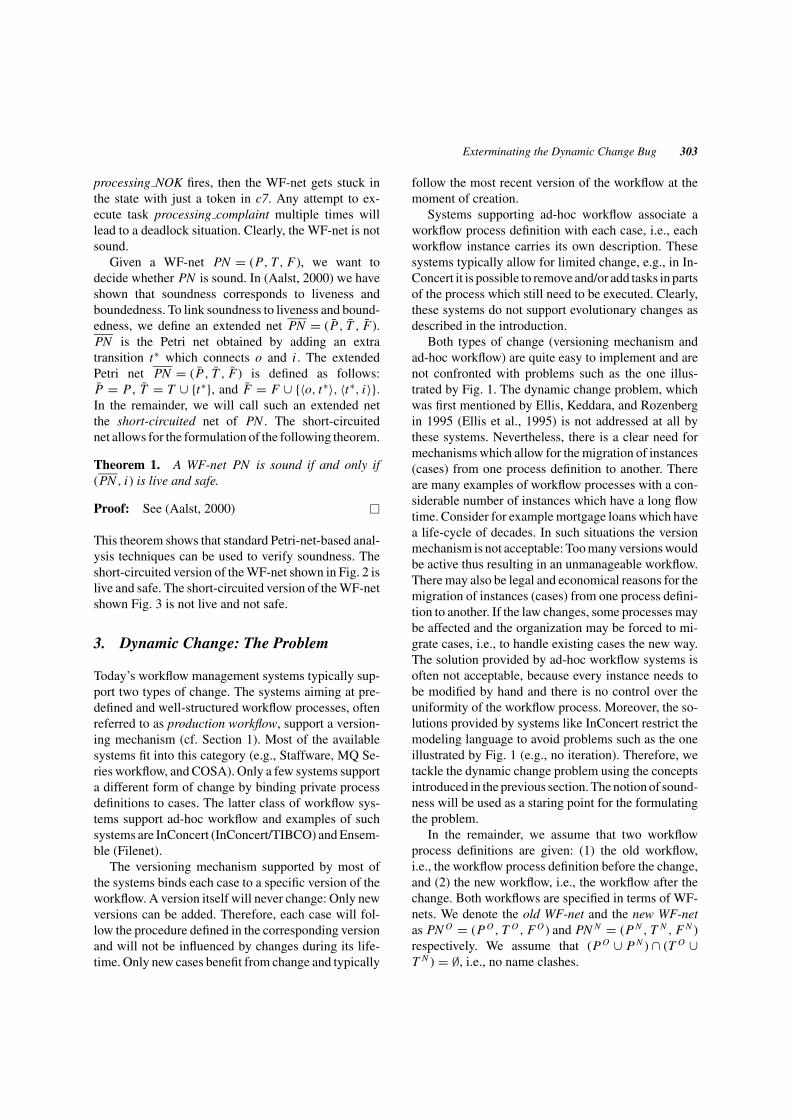
Figs. 7, 8, and 9 show three additional examples.For each example both the dynamic and the staticchange region are indicated. Fig. 7 shows the addi-tion of an alternative branch containing tasks e andf . The static change region SC = {s2, s4, s6, e, f }only addresses the places s2 and s4 in PN O . Thedynamic change region also includes b, s3, and c,

Fig. 7. An old and a new WF-net: SC = {s2, s4, s6, e, f } and DC ={s2, s3, s4, s6, b, c, e, f }.

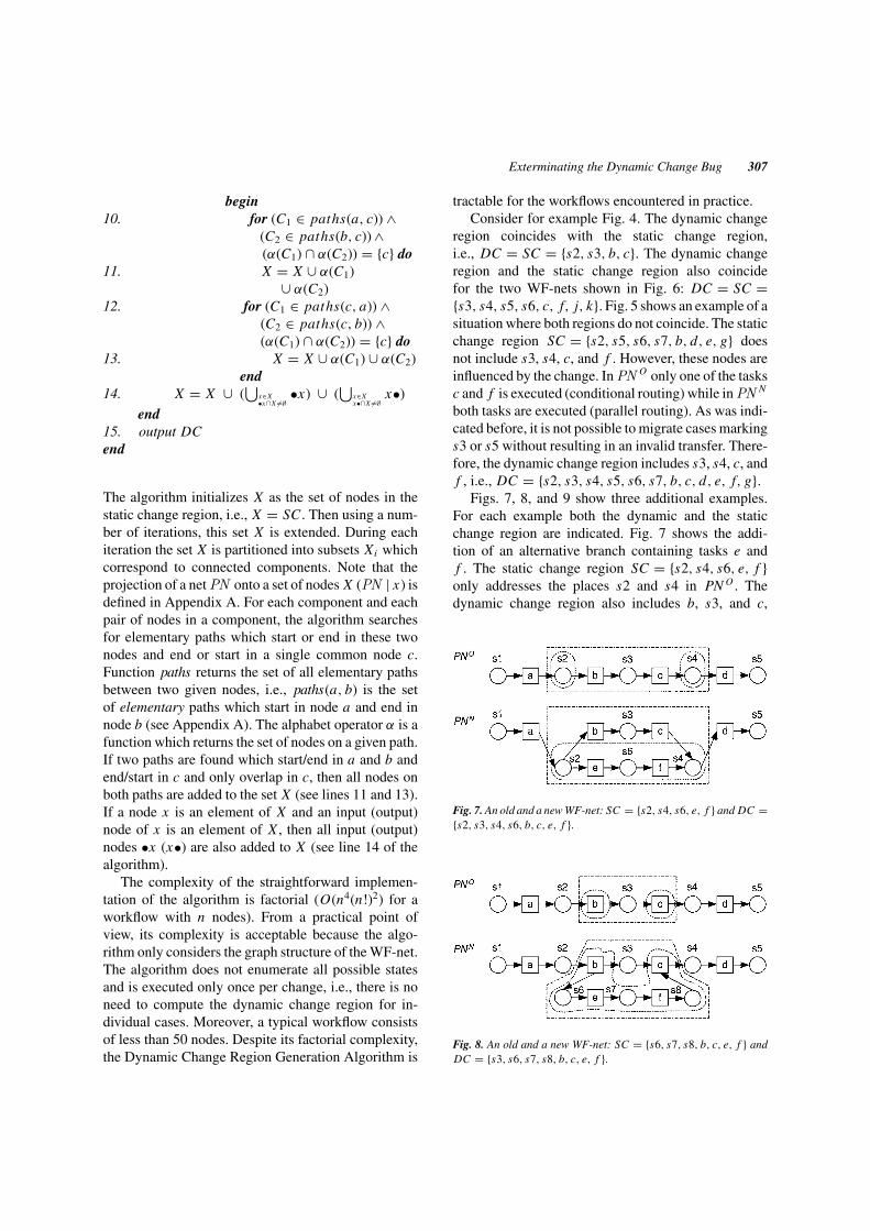
Fig. 8. An old and a new WF-net: SC = {s6, s7, s8, b, c, e, f } andDC = {s3, s6, s7, s8, b, c, e, f }.

308 van der Aalst

Fig. 9. An old and a new WF-net: SC = {s2, s4, e} and DC ={s2, s3, s4, a, b, c, d, e}.

i.e., DC = {s2, s3, s4, s6, b, c, e, f }. Fig. 8 shows theaddition of a parallel branch containing tasks e andf . Place s3 is not included in the static change regionSC = {s6, s7, s8, b, c, e, f }. However, it is clear thats3 also needs to be included. The transfer of a case instate s3 from PN O to PN N results in a deadlock. There-fore, place s3 is included in the dynamic change region,i.e., DC = {s3, s6, s7, s8, b, c, e, f }. Fig. 9 shows theaddition of a feedback loop. This example shows theeffect of line 14 of the algorithm: If a node x is anelement of X and an input (output) node of x is an ele-ment of X , then all input (output) nodes •x (x•) are alsoadded to X . Because of this line the tasks a and d areadded to the dynamic change region. Note that the dy-namic change region DC = {s2, s3, s4, a, b, c, d, e}is considerably larger than the static change regionSC = {s2, s4, e}.

The following theorem shows that the dynamicchange region calculated by the algorithm can be usedto guarantee the validity of transfers, i.e., if only casesoutside the dynamic change region are transferred, thenany transfer is valid.

Theorem 2 (A sufficient condition for valid transfers).Let PN N and PN O be sound WF-nets, PN O N =PN O ∪ PN N , and let DC be the dynamic changeregion. For any reachable marking M of PN O notmarking the dynamic change region, i.e., iPN O

∗→M inPN O and M(p) = 0 for any p ∈ DC ∩ P O , a transfer(PN O , M) ⇒ (PN N , M) is valid.

Proof: See Appendix B �

Consider for example Fig. 6. Theorem 2 guaranteesthat a case marking place s2 can be transferred fromPN O to PN N and vice versa. Note that, just likethe static change region, the dynamic change regionis symmetric. The result of the algorithm does not

depend on the role of PN O and PN N : The two rolescan be reversed without changing the outcome of thealgorithm. Also consider the other examples shown inFigs. 4, 5, 7, 8, and 9. If the dynamic change regionindicated in either PN O or PN N is unmarked, a validtransfer is possible.

The examples given also indicate that Theorem 2provides a sufficient but not necessary condition. Con-sider for example Fig. 6. The dynamic change regionincludes s3, s4, s5, and s6. However, a transfer fromany of these places is valid. The markings with in singletoken in s3, s4, s5, or s6 are reachable from s1 in bothPN O and PN N . The following theorem gives a weakercondition for valid transfers. This theorem is based onthe observation that only the internal places inside thedynamic change region may endanger the validity ofthe transfer. Places on the border of the dynamic changeregion, i.e., places connected to transitions outside DC ,can be marked without compromising the validity of thetransfer.

Theorem 3 (A weaker condition for valid trans-fers). Let PN N and PN O be sound WF-nets,PN O N = PN O ∪ PN N , and let DC be the dynamicchange region. For any reachable marking M of PN O

not marking the internal places of the dynamic changeregion, i.e., iPN O

∗→M in PN O and M(p) = 0 for anyp ∈ {x ∈ DC ∩ P O | (•x) ∪ (x•) ⊆ DC}, a transfer(PN O , M) ⇒ (PN N , M) is valid.

Proof: See Appendix B. �

This theorem shows that we can strengthen the re-sult stated in Theorem 2 quite easily. The set ofplaces considered in Theorem 3 is called the mini-mal change region. The minimal change region MC isdefined as follows: MC = {p ∈ DC | (•x) ∪ (x•) ⊆DC}. The minimal change region includes all nodesof the dynamic change region except the so-calledborder places. Note that the minimal change regionmay be smaller that the static change region. Considerfor example Fig. 4: SC = {s2, s3, b, c} and MC ={s3, b}. The minimal change regions of the exam-ples shown in Figs. 5, 6, 7, 8, and 9 are MC ={s3, s4, s5, s6, b, c, d, e, f, g} (Fig. 5: s2 and s7 areremoved), MC = {c, f, j, k} (Fig. 6: all places areremoved), MC = {s3, s6, b, c, e, f } (Fig. 7: s2 ands4 are removed), MC = {s3, s6, s7, s8, e, f } (Fig. 8:b and c are removed), and MC = {s2, s3, s4, b, c, e}(Fig. 8: a and d are removed) respectively.


In Section 1, Fig. 1 was used to illustrate the dy-namic change problem. We did not refer to this exam-ple in this section because the place identifiers usedin both WF-nets are different. The places in both netshave been named different to avoid confusion whileexplaining the dynamic change problem. However, itis clear that s1 and p1 are in essence the same placebecause their interconnection structures are the same.The same holds for s5 and p6, s2 and p2, s4 and p5.For the remaining places the correspondence is lessclear. Let us rename p1 to s1, p2 to s2, p5 to s4,and p6 to s5 and calculate SC , DC , MC . The staticchange region SC consists of the following nodes:p3, p4, s3, prepare shipment, send goods, send bill,and record shipment. The dynamic change regionDC consists of p3, p4, s2, s3, s4, prepare shipment,send goods, send bill, and record shipment. The min-imal change region MC consists of p3, p4, s2, s3, s4,send goods and send bill.

Finally we illustrate the results using the complaintprocessing example introduced in Section 2.1. Fig. 10shows three potential changes. The first change cor-responds to the removal of task no processing. As-suming this change, the static change region SC con-sists of the following nodes: c4, c6, and no processing.The dynamic change region DC coincides with thestatic change region. The minimal change region MCconsists of only no processing. Hence any transferfrom the WF-net with task no processing to the netwithout no processing and vice versa is valid. The

Fig. 10. Three potential changes.

second change corresponds to the addition of analternative task email questionnaire. Assuming thischange, the static change region SC consists of thefollowing nodes: c1, c3, and email questionnaire.The dynamic change region DC coincides withSC . The minimal change region MC consists ofonly the newly added task. Again any transfer isvalid. The third change is less harmless. If pro-cess complaint is connected directly to c6 and thenodes c8, c9, check processing, processing OK, andprocessing NOK are removed, then the resulting netis a sound WF-net. Assuming this change, the staticchange region SC consists of the following nodes:c6, c7, c8, c9, process complaint, check processing,processing OK, and processing NOK. The dynamicchange region DC encompasses all nodes excepti and o. The minimal change region MC con-sists of all nodes in-between register and archive.Hence only transfers from state i or o are guaran-teed to be valid based on the minimal/dynamic changeregion.

5. Related Work on Dynamic Change

There are many similarities between dynamic changein the workflow domain and schema evolution inthe database domain. As the requirements of databaseapplications change over time, the definition of theschema, i.e., the structure of the data elements stored

310 van der Aalst

in the database, is changed. Schema evolution hasbeen an active field of research in the last decade(mainly in the field of object-oriented databases, cf.Bertino and Martino, 1993) and has resulted in tech-niques and tools that partially support the transfor-mation of data from one database schema to another.Although dynamic change and schema evolution aresimilar, there are some additional complications in caseof dynamic change. First, as was shown in the exam-ple of Fig. 1, it is not always possible to transfer acase. Second, it is not acceptable to shut down thesystem, transfer all cases, and restart using the newprocedure. Cases should be migrated while the sys-tem is running. Finally, dynamic change may introducedeadlocks and livelocks. The solutions provided by to-day’s object-oriented databases do not deal with thesecomplications. Therefore, we need new concepts andtechniques.

Several researchers have worked on problemsrelated to dynamic change. Ellis, Keddara, andRozenberg (1995) propose a technique based on so-called “change regions.” A change region contains allparts of a workflow process definition that potentiallycause problems with respect to the transfer of cases. Achange region has two versions; the old situation andthe new situation. In this solution, there is one versionof the complete process which covers the old and thenew situation and changes affect cases as soon as possi-ble. Parts of the workflow (i.e., change regions) becomeinactive after a while, because all old cases have beenhandled. This approach has the drawback that the pro-cess definition can become very complex (unless someautomatic garbage collection is added). Another draw-back is the fact that the authors do not provide a methodfor identifying the change region, i.e., change regionsneed to be identified manually. The authors do providea notion of change correctness and give specific cir-cumstances for which this is guaranteed. In Ellis andKeddara (2000a), the authors improve their approachby introducing jumpers. A jumper moves a case fromthe old workflow to the new workflow. The jump is post-poned if for a state no jumper is available. Again, theauthors do not give a concrete technique for the trans-fer of cases, i.e., jumpers are added manually. In Ellisand Keddara (2000b) and Keddara (1999), Keddara andEllis present a language to support dynamic evolutionwithin workflow systems (ML-DEWS). Based on thedifferent modalities of change, the authors give a spe-cial purpose meta-language geared to model the work-flow of change. Agostini and De Michelis (2000) pro-

pose a technique for the automatic transfer of casesfrom an old process definition to a new process defi-nition and also give criteria for determining whether atransfer is possible. The approach is interesting sinceit automatically computes the states for which it is notpossible to migrate. Consider for example Fig. 1. Theapproach presented in Agostini and Michelis (2000)indicates the necessity to postpone the transfer of run-ning cases in state [p1, p4]. Unfortunately, the ap-proach only works for a restricted class of workflows(e.g., the modeling language does not allow for iter-ation, although at runtime iteration can be achievedby backward jumps). A summary of this approach isgiven in Michelis and Ellis (1998). Weske (Vossen andWeske, 1999; Weske, 2000) considers dynamic work-flow change using a model similar to the model usedby IBM’s MQSeries. In this model there is no iterationand also alternatives are synchronized. As a result thecontrol flow is similar to a subclass of Petri nets:the so-called acyclic marked graphs. By exploitingthese restrictions, relatively simple criteria can be ob-tained to guarantee the proper migration of an instancefrom one schema to another (Weske, 2000). Joeris andHerzog use linked State Charts to address the prob-lem of posteriori flexibility (Joeris and Herzog, 1998).Casati, Ceri, and Pernici (1998) tackle the problem ofdynamic change via a set of transformation rules andpartition the state space into a part that is aborted, a partthat is transferred, a part that is handled the old way,and parts which are handled by hybrid process defini-tions (similar to the approach using change regions).Reichert and Dadam (1998) use a similar approach.However, semantical issues such as errors introducedby swapping tasks, skipping tasks, or multiple execu-tions of a task are not considered. Voorhoeve and Vander Aalst (1996, 1997) also propose a fixed set of trans-formation rules to support dynamic change. However,the rules are not given explicitly at the net level and se-mantical issues are not considered. Van der Aalst andBasten (2001) propose an approach based on inheri-tance. This approach uses a set of generic inheritance-preserving transformation and transfer rules. Semanti-cal errors such as the swapping of tasks, the skippingof tasks, and the multiple execution of tasks can beavoided by choosing the appropriate inheritance no-tion, e.g., projection inheritance guarantees that taskscannot be skipped by transferring a case from the su-perclass to the subclass. Unfortunately, the approach isnot useful if the new workflow is not a super or subclassof the old workflow. The reader interested in workflow


change and Petri nets is also referred to Aalst, Desel,and Oberweis (2000b) which contains several papers ofthe authors mentioned above. We also refer to the PhDthesis of Keddara (1999) for a more complete overviewof related work on dynamic change.

The strength of the approach presented in thispaper is that it can be applied in the context ofarbitrary changes. Note that we did not assume theabsence of certain routing constructs (i.e., sequen-tial, conditional, parallel, and iterative are included) orrestrict change to specific types of changes. Anotherfeature of the approach is that the change regions are de-termined based on the structure of the workflow model(i.e., syntax) rather than the dynamics (i.e., a state spaceexploration). This facilitates implementation and yieldschange regions which are tangible to end users.

6. Conclusion

This paper provides a pragmatic approach to tackle thedynamic change bug. Based on the syntactic changes inthe graphical workflow model, three types of change re-gions are calculated. The static change region incorpo-rates the parts of the workflow model directly effectedby the change. The dynamic change region extendsthe static change region to incorporate the parts of theworkflow model indirectly effected by the change. Theminimal change region reduces the dynamic change re-gion by eliminating border nodes. The minimal changeregion is a subset of the dynamic change region. Themain result of this paper is that cases (i.e., work-flow instances) which leave the minimal change regionunmarked can be transferred from the old workflowto the new workflow without creating problems suchas deadlocks and livelocks: Successful termination isguaranteed.

In the future, we plan to implement the approachpresented in this paper using a commercial workflowmanagement system. First, we plan to extend the work-flow management system COSA (Thiel/Ley/COSA So-lutions) with a feature to calculate the minimal changeregion and to enact valid transfers. This extension ofCOSA is quite straightforward since COSA is basedon Petri nets and provides an API to remove and cre-ate cases in any state in any workflow. Second, weplan to realize the same functionality using other work-flow management systems. Staffware (Staffware plc)is an example of another system we use in our labo-ratory. Implementation of this feature in Staffware is

less straightforward because Staffware is not based onPetri nets and it is not known whether the requiredAPI is provided. Other candidates for realizing ourapproach are Verve (Verve Inc.) and i-Flow (FujitsuSoftware Corporation). Both systems offer extensiveAPI’s.

Appendix A: Petri Nets

The classical Petri net (Desel and Esparza, 1995;Murata, 1998; Reisig and Rozenberg, 1998) is adirected bipartite graph with two node types calledplaces and transitions. The nodes are connected viadirected arcs. Connections between two nodes of thesame type are not allowed. Places are represented bycircles and transitions by rectangles.

Definition 6 (Petri net). A Petri net is a triple(P, T, F):

– P is a finite set of places,– T is a finite set of transitions (P ∩ T = ∅),– F ⊆ (P × T ) ∪ (T × P) is a set of arcs (flow rela-

tion)

A place p is called an input place of a transition t iffthere exists a directed arc from p to t . Place p is calledan output place of transition t iff there exists a directedarc from t to p. We use •t to denote the set of inputplaces for a transition t . The notations t•, •p and p•have similar meanings, e.g., p• is the set of transitionssharing p as an input place. Note that we do not considermultiple arcs from one node to another. In the contextof workflow procedures it makes no sense to have otherweights, because places correspond to conditions.

To illustrate there concepts we consider the twoPetri nets shown in Fig. 1. The Petri net on the lefthas four transitions and five places. The Petri net onthe right has four transitions and six places. Transitionprepare shipment in the left model has one input placeand two output places. Note that p1 and s1 are sourceplaces, i.e., places without any input transition. Placess5 and p6 are sink places.

At any time a place contains zero or more to-kens, drawn as black dots. The state, often referredto as marking, is the distribution of tokens overplaces, i.e., M ∈ P → N. We will represent a state asfollows: 1p1 + 2p2 + 1p3 + 0p4 is the state with onetoken in place p1, two tokens in p2, one token in p3

and no tokens in p4. We can also represent this state

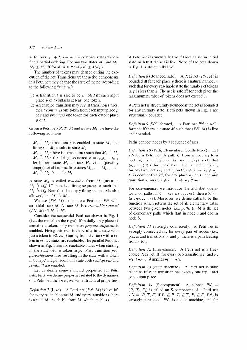
312 van der Aalst

as follows: p1 + 2p2 + p3. To compare states we de-fine a partial ordering. For any two states M1 and M2,M1 ≤ M2 iff for all p ∈ P : M1(p) ≤ M2(p).

The number of tokens may change during the exe-cution of the net. Transitions are the active componentsin a Petri net: they change the state of the net accordingto the following firing rule:

(1) A transition t is said to be enabled iff each inputplace p of t contains at least one token.

(2) An enabled transition may fire. If transition t fires,then t consumes one token from each input place pof t and produces one token for each output placep of t .

Given a Petri net (P, T, F) and a state M1, we have thefollowing notations:

– M1t→ M2: transition t is enabled in state M1 and

firing t in M1 results in state M2

– M1 → M2: there is a transition t such that M1t→ M2

– M1σ→ Mn: the firing sequence σ = t1t2t3 . . . tn−1

leads from state M1 to state Mn via a (possiblyempty) set of intermediate states M2, . . . , Mn−1, i.e.,M1

t1→ M2t2→ · · · tn−1→ Mn

A state Mn is called reachable from M1 (notationM1

∗→ Mn) iff there is a firing sequence σ such thatM1

σ→ Mn . Note that the empty firing sequence is alsoallowed, i.e., M1

∗→ M1.We use (PN , M) to denote a Petri net PN with

an initial state M . A state M ′ is a reachable state of(PN , M) iff M

∗→ M ′.Consider the sequential Petri net shown in Fig. 1

(i.e., the model on the right). If initially only place s1contains a token, only transition prepare shipment isenabled. Firing this transition results in a state withjust a token in s2, etc. Starting from the state with a to-ken in s1 five states are reachable. The parallel Petri netshown in Fig. 1 has six reachable states when startingin the state with a token in p1. First transition pre-pare shipment fires resulting in the state with a tokenin both p2 and p3. From this state both send goods andsend bill are enabled.

Let us define some standard properties for Petrinets. First, we define properties related to the dynamicsof a Petri net, then we give some structural properties.

Definition 7 (Live). A Petri net (PN , M) is live iff,for every reachable state M ′ and every transition t thereis a state M ′′ reachable from M ′ which enables t .

A Petri net is structurally live if there exists an initialstate such that the net is live. None of the nets shownin Fig. 1 is structurally live.

Definition 8 (Bounded, safe). A Petri net (PN , M) isbounded iff for each place p there is a natural number nsuch that for every reachable state the number of tokensin p is less than n. The net is safe iff for each place themaximum number of tokens does not exceed 1.

A Petri net is structurally bounded if the net is boundedfor any initially state. Both nets shown in Fig. 1 arestructurally bounded.

Definition 9 (Well-formed). A Petri net PN is well-formed iff there is a state M such that (PN , M) is liveand bounded.

Paths connect nodes by a sequence of arcs.

Definition 10 (Path, Elementary, Conflict-free). LetPN be a Petri net. A path C from a node n1 to anode nk is a sequence 〈n1, n2, . . . , nk〉 such that〈ni , ni+1〉 ∈ F for 1 ≤ i ≤ k − 1. C is elementary iff,for any two nodes ni and n j on C, i = j ⇒ ni = n j .C is conflict-free iff, for any place n j on C and anytransition ni on C , j = i − 1 ⇒ n j ∈ •ni .

For convenience, we introduce the alphabet opera-tor α on paths. If C = 〈n1, n2, . . . , nk〉, then α(C) ={n1, n2, . . . , nk}. Moreover, we define paths to be thefunction which returns the set of all elementary pathsbetween two given nodes, i.e., paths (a, b) is the setof elementary paths which start in node a and end innode b.

Definition 11 (Strongly connected). A Petri net isstrongly connected iff, for every pair of nodes (i.e.,places and transitions) x and y, there is a path leadingfrom x to y.

Definition 12 (Free-choice). A Petri net is a free-choice Petri net iff, for every two transitions t1 and t2,•t1 ∩ •t2 = ∅ implies •t1 = •t2.

Definition 13 (State machine). A Petri net is statemachine iff each transition has exactly one input andone output place.

Definition 14 (S-component). A subnet PN s =(Ps, Ts, Fs) is called an S-component of a Petri netPN = (P, T, F) if Ps ⊆ P , Ts ⊆ T , Fs ⊆ F , PN s isstrongly connected, PN s is a state machine, and for


every q ∈ Ps and t ∈ T : (q, t) ∈ F ⇒ (q, t) ∈ Fs and(t, q) ∈ F ⇒ (t, q) ∈ Fs .

Definition 15 (S-coverable). A Petri net is S-coverable iff for any node there exist an S-componentwhich contains this node.

See Desel and Esparza (1995) and Reisig andRozenberg (1998) for a more elaborate introduction tothese standard notions. In addition to these standardnotions we also define the some operators on nets,i.e., the union of two nets, the subnet notion, and theprojection of a net onto a set of places and transitions.

Definition 16 (Union, subnet). Let PN 1 = (P1, T1,

F1) and PN 2 = (P2, T2, F2) be two Petri nets. Theunion of PN 1 and PN 2 is a Petri net PN PN1∪PN2 =PN1 ∪ PN2, where PPN1∪PN2 = P1 ∪ P2, TPN1 ∪ PN2 =T1 ∪ T2, and FPN1 ∪ PN2 = F1 ∪ F2. PN 1 is a subnet ofPN 2, denoted as PN 1 ⊆ PN2, iff P1 ⊆ P2, T1 ⊆ T2,and F1 ⊆ F2.

Definition 17 (Projection). Let PN = (P, T, F) aPetri net and X ⊆ P ∪ T . The projection of PN ontoX is PN |X = (P ∩ X, T ∩ X, F ∩ (X × X )).

The projection of a Petri net onto a set of nodes in-cludes all connections between these nodes, i.e., iftwo nodes are connected in PN and are both in-cluded in X , then these nodes are also connected inPN |X . Note that, by definition, PN |X is a subnet ofPN .

Appendix B: Proof of Theorems 2 and 3

In this appendix we will show that the dynamic changeregion indeed provides a criterion which is sufficient toguarantee the validity of transfers. The essence of theproof uses the fact that each component Xi identifiedby the algorithm is similar to a sound WF-net, i.e., aconnected set of nodes with one unique source nodeand one unique sink node whose composite behavioris comparable to a single transition. To prove thecentral theorem of this paper we need to introducecomponents and source and sink nodes.

Definition 18 (Source and sink nodes). LetPN = (P, T, F) be a Petri net and X ⊆ P ∪ T .source(PN , X ) is the set of source nodes of Xand is defined as follows: source(PN , X ) = {x ∈X | • x ∩ X = ∅}. sink (PN , X ) is the set of

sink nodes of X and is defined as follows: sink(PN , X ) = {x ∈ X | x • ∩ X = ∅}.A source node is either a node without any input nodesor a node with only external input nodes. Consider forexample Fig. 4. Place s2 is the only source node ofSC in PN O . A sink node is either a node without anyoutput nodes or a node with only external output nodes.Consider for example Fig. 9. Place s2 is the only sinknode of SC in PN N . Both s2 and s4 are source andsink nodes of SC in PN O .

Based on the notions of source and sink nodes wedefine components.

Definition 19 (Component). Let PN = (P, T, F) bea Petri net and X ⊆ P ∪ T . X is a component of PNif and only if:

(i) source(PN , X ) is a singleton, i.e., there is an a suchthat {a} = source(PN , X ),

(ii) sink(PN , X ) is a singleton, i.e., there is a b suchthat {b} = sink(PN , X ),

(iii) for each x ∈ X : x is on a directed path from a to b,(iv) for each elementary path C from a to b (i.e., C ∈

paths(a, b)): α(C) ⊆ X .

Components are similar to WF-nets embedded in alarger Petri net. However, in contrast to WF-nets, thesource/sink node can be a transition instead of a place.

In line 5 of the algorithm the set X is partitionedinto subsets Xi . The goal of the algorithm is toextend X such that these subsets correspond to com-ponents. The following lemma lists eight propertiesof the Xi components constructed by the algorithm.These properties will be used in the proof of Theorem 2.

Lemma 1. Let PN N and PN O be sound WF-nets,PN O N = PN O ∪ PN N , and let DC be the dynamicchange region. Let DC be partitioned into X1, X2,

. . . , Xn such that:

(a) Xi ∩ X j = ∅ for all 1 ≤ i < j ≤ n(b) DC = ⋃

1≤i≤n Xi

(c) PN O N |Xi is connected for all 1 ≤ i ≤ n(d) (•Xi ) ∩ X j = ∅ and (Xi•) ∩ X j = ∅ for all 1 ≤

i < j ≤ n

Such partitioning always exists and is unique. The par-titioning has the following properties:

(e) For all 1 ≤ i ≤ n: Xi is a component of PN O N .( f ) For all 1 ≤ i ≤ n: Xi ∩ (P O ∪ T O ) is a component

of PN O .

314 van der Aalst

(g) For all 1 ≤ i ≤ n: Xi ∩ (P N ∪ T N ) is a componentof PN N .

(h) For all 1 ≤ i ≤ n: source(PN ON , Xi ) = source(PN O , Xi ∩ (P O ∪ T O )) = source (PN N , Xi ∩(P N ∪ T N )) and sink(PN ON , Xi ) = sink(PN O ,

Xi ∩ (P O ∪ T O )) =sink (PN N , Xi∩ (P N ∪ T N )).

Proof: First we prove that DC can be partitioned ininto X1, X2, . . . , Xn and that this partitioning is unique.Partition DC into singletons X1, X2, . . . , Xm . Such apartitioning satisfies properties (a), (b), and (c). If thepartitioning does not satisfy property (d), then there isan i and j such that there is an arc from a node in Xi

to a node in X j . If this is the case, then join Xi and X j .Clearly the nodes Xi ∪ X j are connected. Then repeatthe procedure until (d) holds. Note that the existenceof such a partition is used in line 5 of the algorithm.

It remains to be proven that properties (e), (f ), (g),and (h) hold. We will prove these properties for a givenset of nodes Xi (1 ≤ i ≤ n) identified in the partition-ing.

The algorithm stops if no new nodes are added inlines 6 through 14. This implies that at the end:

(i) For all a ∈ Xi , b ∈ Xi \ {a}, c ∈ P ON ∪ T ON ,C1 ∈ paths(a, c), C2 ∈ paths(b, c) such thatα(C1) ∩ α(C2) = {c}: α(C1) ∪ α(C2) ⊆ Xi .

(ii) For all a ∈ Xi , b ∈ Xi \ {a}, c ∈ P ON ∪ T ON ,C1 ∈ paths(c, a), C2 ∈ paths(c, b) such thatα(C1) ∩ α(C2) = {c} : α(C1) ∪ α(C2) ⊆ Xi .

(iii) For all x ∈ Xi such that •x ∩ Xi = ∅ : •x ⊆ Xi ,i.e., •x ⊆ Xi implies x ∈ source(PN ON , Xi ).

(iv) For all x ∈ Xi such that x• ∩ Xi = ∅ : x• ⊆ Xi ,i.e., x• ⊆ Xi implies x ∈ sink(PN ON , Xi ).

The first two observations follow directly from thealgorithm. The latter two are the result of line 14 inthe algorithm and property (d). These observations areused to prove the remaining properties.

Property (e). First we prove that source (PN ON , Xi )is a singleton. There is at least one source node. IfXi contains iPN O N , then iPN O N is a source node. If Xi

does not contain iPN O N , then there is a directed pathfrom iPN O N to a node in Xi . Consider the first node ofXi on this path. Clearly this node is a source nodeof Xi (use Property (iii)). There cannot be two sourcenodes. Suppose that both a and b are source nodesof Xi and a = b. There is a directed elementary pathfrom iPN O N to a and from iPN O N to b. Let c be the last

common node of these two paths, i.e., walk backwardson the directed elementary path from iPN O N to a untilone encounters a node also appearing in the other path.Based on these two paths and the last common node,we define two subpaths: an elementary directed pathC1 from c to a, and an elementary directed path C2

from c to b. Clearly, (α(C1) ∩ α(C2)) = {c}. Hence,(α(C1) ∪ α(C2)) ⊆ Xi (use Observation (i) and {c} ⊆Xi ). However, since both a and b are source nodes ofXi , there cannot be any input nodes from within Xi .Hence, both paths cannot contain multiple nodes, i.e.,c = a and c = b. This contradicts the assumption thata = b and shows that there can only be one sourcenode.

Similarly, it can be shown that sink(PN ON , Xi ) is asingleton.

Let {a} = source(PN ON , Xi ), {b} = sink(PN O N ,

Xi ), and x ∈ Xi . We need to prove that x is on a di-rected path from a to b. Let C1 be a directed path fromiPN O N to x and C2 be a directed path from x to oPN ON .Such paths exist since PN ON is a WF-net. Let y be thefirst element of Xi on C1. Clearly y = a (use Observa-tion (iii)). Hence, there is a directed path from a to x .Similarly, it can be shown that there is a directed pathfrom x to b.

Let C be an elementary path from a to b. Observa-tion (i) implies that α(C) ⊆ Xi (b = c).

Property (f). Let a be the unique source node of Xi

in PN ON , i.e., {a} = source (PN ON , Xi ). a is also anode of PN O : either a = iPN ON which also appears inPN O or there is a node x not in DC such that x ∈ •a.In the latter case x is not in the static change region(SC ⊆ DC) and therefore the set of nodes connectedto x did not change. Hence a is a node of PN O . SincePN O is a subnet of PN ON , a is also a source nodeof Xi in PN O . Note that only by adding new connec-tions source nodes can become non-source nodes. Sim-ilarly, we can show that the unique sink node b of Xi inPN ON , i.e., {b} = sink(PN ON , Xi ), is also a sink nodeof PN O .

a is a source node of Xi in PN O and b is a sinknode of Xi in PN O . Before we show that these twonodes are unique, we focus on the other two propertiesa component needs to satisfy.

Every node x in Xi is on a path from a to b in PN ON

(see proof of Property (e)). If x ∈ Xi is a node of PN O ,then x is on a path from a to b in PN O . Let C1 be adirected path from iPN O to x and C2 be a directed pathfrom x to oPN O in PN O . Such paths exist since PN O is


a WF-net and both paths are also paths of PN ON . Is iseasy to show that a must appear on path C1 (considerthe first node of Xi ; this must be a) and b must appearon C2.

Let C be a directed path from a to b in PN O . Cis also a path in PN ON . Clearly, α(C) ⊆ Xi (see proofof Property (e)). Since C be a directed path in PN O ,α(C) ⊆ Xi ∩ (P O ∪ T O ).

It remains to be proven that a and b are unique.Suppose there is an additional source node x , i.e., x ∈source(PN O , Xi ∩ (P O ∪ T O )) and x = a. Since x ison a directed path from a to b contained in Xi ∩ (P O ∪T O ), x cannot be source node, i.e., a is the only sourcenode. Similarly, it can be shown that b is unique.

Based on these observations we conclude that Xi ∩(P O ∪ T O ) is a component of PN O .

Property (g). The proof of this property is identical tothe proof of Property (f ).

Property (h). This property follows directly from theproof of properties (f ) and (g). �

Based on the eight properties listed in Lemma 1, weprove Theorem 2. This theorem states that the dynamicchange region provides a sufficient condition for validtransfers.

Theorem (A sufficient condition for valid transfers).Let PN N and PN O be sound WF-nets, PN ON =PN O ∪ PN N , and let DC be the dynamic changeregion. For any reachable marking M of PN O notmarking the dynamic change region, i.e., iPN O

∗→M inPN O and M(p) = 0 for any p ∈ DC ∩ P O , a transfer(PN O , M) ⇒ (PN N , M) is valid.

Proof: Let M be such that iPN O∗→ M in PN O and

M(p) = 0 for any p ∈ DC ∩ P O .First, we prove that for all p ∈ P O : M(p) ≥ 1 im-

plies p ∈ P N . If p ∈ P O and M(p) ≥ 1, then p ∈ DC .Hence, p ∈ SC (SC ⊆ DC). Property 1 shows that(P O ∪ T O ) \ (P N ∪ T N ) ⊆ SC . Therefore, p ∈ P N .

Finally, we prove that iPN N∗→ M in PN N .

Lemma 1 shows that DC can be partitioned intoX1, X2, . . . , Xn such that Xi is a component ofPN ON , Xi ∩ (P O ∪ T O ) is a component of PN O , andXi ∩ (P N ∪ T N ) is a component of PN N . Consider anarbitrary component Xi with {a} = source(PN ON , Xi )and {b} = sink(PN ON , Xi ). If both a and b areplaces, then PN ON |Xi , PN O |Xi , and PN N |Xi are

WF-nets. This follows directly from Definition 6.Since PN ON |Xi , PN O |Xi , and PN N |Xi are subnets ofsound WF-nets, these subnets are also sound. (SeeTheorem 3 in Aalst (2000).) Note that the soundnessof each subnet heavily depends on the safeness ofthe enclosing WF-net. Since the subnets are soundtheir behavior corresponds to a single transition tv

connecting a and b. Now consider firing sequence σ

which leads to M in PN O , i.e., iPN Oσ→M . Consider

the transitions of Xi which occur in σ . These transitionform complete subsequences of the embedded WF-netPN O |Xi , i.e., since no tokens are left in Xi everysubsequence corresponds one firing of the virtualtransition tv . Each firing of this virtual transition canbe mimicked by a firing sequence of the embeddedWF-net PN N |Xi in PN N . This way occurrences oftransitions in Xi ∩ T O can be replaced by transitionsin Xi ∩ T N . This assumes that both a and b areplaces. However, the same reasoning can be appliedto components where a and/or b are transitions. Sucha transition-bordered WF-net can be transformed intoa sound WF-net by adding a source and/or sink place.This can be repeated for each of the components.Therefore, σ can be transformed into a firing sequenceσ ′ which leads to M in PN N , i.e., iPN O

σ ′→M . Hence,iPN N

∗→M in PN N . �

Finally we prove Theorem 3.

Theorem (A weaker condition for valid transfers).Let PN N and PN O be sound WF-nets, PN ON =PN O ∪ PN N , and let DC be the dynamic changeregion. For any reachable marking M of PN O notmarking the internal places of the dynamic changeregion, i.e., iPN O

∗→M in PN O and M(p) = 0 for anyp ∈ {x ∈ DC ∩ P O | (•x) ∪ (x•) ⊆ DC}, a transfer(PN O , M) ⇒ (PN N , M) is valid.

Proof: Compared to Theorem 2 so-called borderplaces p can be marked while a case is beingtransferred. Consider a place p ∈ DC ∩ P O suchthat not (•p) ∪ (p•) ⊆ DC , i.e., •p ⊆ DC or p• ⊆DC . If •p ⊆ DC , then {p} = source(PN ON , Xi ) =source(PN O , Xi ) = source(PN N , Xi ) of some com-ponent Xi . Since p appears in PN O and PN N , thesets of input transitions of p are identical in PN O andPN N , and PN O |Xi and PN N |Xi have a behavior simi-lar to a single transition, a transfer of a token in p doesnot jeopardize the validity of the transfer. Similarly, a

316 van der Aalst

token in a place p with p• ⊆ DC cannot jeopardizethe validity. Hence, if only places outside DC and bor-der places are marked, then (PN O , M) ⇒ (PN N , M)is valid. �

Acknowledgments

Part of the work reported in this paper was con-ducted while the author was visiting the Large ScaleDistributed Information Systems (LSDIS) Laboratory,Department of Computer Science, University ofGeorgia, Athens, USA. The author would like to thankIsmael Budak Arpinar of the LSDIS lab. for his inputduring this visit, and Eric Verbeek for proofreading thepaper.

Note

1. Note that there is an overloading of notation: the symbol i is usedto denote both the place i and the state with only one token inplace i (see Appendix A).

References

Aalst W van der. Three good reasons for using a Petri-net-basedworkflow management system. In: Wakayama T, Kannapan S,Khoong C, Navathe S, Yates J, eds. Information and Process Inte-gration in Enterprises: Rethinking Documents, The Kluwer Inter-national Series in Engineering and Computer Science, Vol. 428, ch.100, Boston: Kluwer Academic Publishers, Massachusetts, 1998a:161–182.

Aalst W van der. The application of Petri nets to workflowmanagement. The Journal of Circuits, Systems and Computers1998b;8(1):21–66.

Aalst W van der. workflow verification: Finding control-flow er-rors using Petri-net-based techniques. In: Business Process Man-agement: Models, Techniques, and Empirical Studies, LectureNotes in Computer Science, Vol. 1806. Berlin: Springer-Verlag,2000:161–183.

Aalst W van der, Basten T. Inheritance of workflows: An approachto tackling problems related to change. Theoretical Computer Sci-ence 2001 (to appear).

Aalst W van der, Basten T, Verbeek H, Verkoulen P, Voorhoeve M.Adaptive workflow: On the interplay between flexibility and sup-port. In: Filipe J, ed. Enterprise Information Systems. Norwell:Kluwer Academic Publishers, 2000a:63–70.

Aalst W van der, Desel J, Oberweis A. (eds.) Business ProcessManagement: Models, Techniques, and Empirical Studies, LectureNotes in Computer Science, Vol. 1806. Berlin: Springer-Verlag,2000b.

Agostini A, Michelis G. Improving flexibility of workflow manage-ment systems. In: W van der Aalst, Pesel J, Oberweis A, eds.Business Process Management: Models, Techniques, and Empiri-cal Studies, Lecture Notes in Computer Science, Vol. 1806. Berlin:Springer-Verlag, 2000:218–234.

Bertino E, Martino L. Object-Oriented Database Systems: Conceptsand Architecture. Addison-Wesley, Reading MA (1993).

Casati F, Ceri S, Pernici B, Pozzi G. workflow evolution. Data andKnowledge Engineering 1998;24(3):211–238.

Desel J, Esparza J. Free Choice Petri Nets, Cambridge Tracts in The-oretical Computer Science, Vol. 40. Cambridge, UK: CambridgeUniversity Press, 1995.

Ellis C, Keddara K. A workflow change is a workflow. In: Busi-ness Process Management: Models, Techniques, and EmpiricalStudies, Lecture Notes in Computer Science, Vol. 1806. Berlin:Springer-Verlag, 2000a:201–217.

Ellis C, Keddara K. ML-DEWS: Modeling language to support dy-namic evolution within workflow systems. Computer SupportedCooperative Work 2000b; 9(3/4): 293–333.

Ellis C, Keddara K, Rozenberg G. Dynamic change within work-flow systems. In: Comstock N, Ellis C, Kling R, Mylopoulos J,Kaplan S, eds. Proceedings of the Conference on OrganizationalComputing Systems, Milpitas, California. ACM SIGOIS. NewYork: ACM Press, 1995:10–21.

Ellis C, Nutt G. Modelling and enactment of workflow systems. In:Marsan, M A, ed. Application and Theory of Petri Nets 1993,Lecture Notes in Computer Science, Vol. 691. Berlin: Springer-Verlag, 1993:1–16.

Gostellow K, Cerf V, Estrin G, Volansky S. Proper termination offlow-of-control in programs involving concurrent processes. ACMSigplan 1972;7(11):15–27.

Jablonski S. Bussler C. workflow Management: Modeling Con-cepts, Architecture, and Implementation. London, UK: Interna-tional Thomson Computer Press, 1996.

Joeris G, Herzog O. Managing evolving workflow specifica-tions. In: Proceedings of the 3rd IFCIS International Con-ference on Cooperative Information Systems, 20–22 AugustNew York City, New York, USA: IEEE-CS Press, 1998:310–321.

Keddara K. Dynamic evolution of workflow systems. PhD Thesis,University of Colorado, Boulder, Colorado, USA, 1999.

Kindler E, Aalst W. Liveness, fairness, and recurrence. InformationProcessing Letters 1999;70(6):269–274.

Koulopoulos T. The workflow Imperative. New York: Van NostrandReinhold, 1995.

Lawrence P. (ed.) workflow Handbook 1997, workflow ManagementCoalition. New York: Wiley, 1997.

Michelis G. De, Ellis C. Computer supported cooperative work andPetri nets. In: Reisig W, Rozenberg G, eds. Lectures on Petri NetsII: Applications, Lecture Notes in Computer Science, Vol. 1492.Berlin: Springer-Verlag, 1998:125–153.

Murata T. Petri nets: Properties, analysis and applications. Proceed-ings of the IEEE 1998;77(4):541–580.

Reichert M, Dadam P. ADEPTflex: Supporting dynamic changes ofworkflow without loosing control. Journal of Intelligent Informa-tion Systems 1998;10(2):93–129.

Reisig W, Rozenberg G. (eds.) Lectures on Petri Nets I: Basic Models,Lecture Notes in Computer Science, Vol. 1491. Berlin: Springer-Verlag, 1998.


Sadiq S, Marjanovic O, Orlowska M. Managing change and time indynamic workflow processes. International Journal of Coopera-tive Information Systems 2000;9(1-2):93–116.

Voorhoeve M. Aalst W van der. Conservative adaption of work-flow. In: Wolf M, Reimer U, eds. Proceedings of the Inter-national Conference on Practical Aspects of Knowledge Man-agement (PAKM’96), Workshop on Adaptive workflow, Basel,Switzerland, 1996: 1–15.

Voorhoeve M, Aalst W van der. Ad-hoc workflow: Problems andsolutions. In Wagner R., ed. Proceedings of the 8th DEXA Inter-national Workshop on Database and Expert Systems Applications,Toulouse, France. Los Alamitos, California: IEEE Computer So-ciety Press, 1997:36–40.

Vossen G, Weske M. The WASA2 object-oriented workflow man-agement system. In: Delis A. Faloutsos C, GhandeharizadehS, ed. SIGMOD 1999, Proceedings ACM SIGMOD Inter-national Conference on Management of Data, 1–3 June,1999, Philadelphia, Pennsylvania, USA: ACM Press, 1999:587–589.

Weske M. Foundation, design, and implementation of dynamicadaptations in a workflow management system. FachberichtAngewandte Mathematik und Informatik 6/2000-I, Universitat

Munster, Munster, Germany, 2000WFMC workflow management coalition terminology and glos-

sary (WFMC-TC-1011). Technical report, workflow ManagementCoalition, Brussels, 1996.

Wil van der Aalst is a full professor of InformationSystems and head of the Department of Informationand Technology of the Faculty of Technology Man-agement of Eindhoven University of Technology. Heis also a part-time professor at the Computing Sciencedepartment of the same university and has been work-ing as a part-time consultant for Bakkenist for sev-eral years. His research interests include informationsystems, simulation, Petri nets, process models, workmanagement systems, verification techniques, enter-prise resource planning systems, computer supportedcooperative work, and interorganizational businessprocesses.

Exterminating the dynamic change bug: A concrete … · Exterminating the Dynamic Change Bug 299 in...

Documents

Transcript of Exterminating the dynamic change bug: A concrete … · Exterminating the Dynamic Change Bug 299 in...