Extensive Form Games - College of Arts and Sciences

CHAPTER 2

Extensive Form Games

Again, we begin our discussion of extensive form games without defining whatone is, but giving some examples.

1. Examples of extensive form games

1

4

32

L R

A BDU

X Y X Y

4, 3, 7, 11 2, 9, 16, 3 10, 1, 9, 8 1, 10, 8, 9

1, 1, 1, 11, 1, 1, 1

Figure 1. An extensive form game.

Look at Figure 1. We interpret this as follows. Each point where a player getsto move in the game or at which the game ends is called a node. Nodes at whichplayers move are shown by small black dots in Figure 1 and are called decisionnodes. The game starts at a particular node, called the initial node or root. Inthis case we assume that the lowest node where Player 1 moves is the initial node.Player 1 chooses between L or R. If Player 1 chooses L then Player 2 moves andchooses between U or D. If Player 1 chooses R then Player 3 moves and choosesbetween A and B. If Player 2 chooses U then the game ends. If Player 2 chooses Dthen player 4 moves. If player 3 chooses B then the game ends. If player 3 choosesA then Player 4 moves. When it’s Player 4’s turn to move, he doesn’t see whetherhe is called upon to move because Player 1 chose L and Player 2 chose D or becausePlayer 1 chose R and Player 3 chose A. We say that the two nodes at which player4 moves are in the same information set and we represent this by joining them witha dotted line as in Figure 1. If it’s player 4’s turn to move, he chooses between Xand Y , after which the game ends. The nodes at which the game ends are calledterminal nodes. To each terminal node we associate a payoff to each player. Thesepayoffs tell us how the player evaluates the game ending at that particular node,that is they tell us the players’ preferences over the terminal nodes, as well as theirpreferences over randomisations over those nodes.

23

24 2. EXTENSIVE FORM GAMES

Nature

1

12

12

12

In OutINOUT

S D S D

−2, 2 2,−2 2,−2 −2, 2

−1, 11,−1

Figure 2. Another extensive form game. This game does nothave perfect recall.

As another example, consider the extensive form game shown in Figure 2. Inthis game, the first mover is not a player but “Nature”. That is, at the beginning ofthe game, there is a random selection of whether Player 1 or Player 2 gets to move,each being chosen with probability 1

2 . (I shall indicate such moves of Nature by anopen circle, while nodes at which real players move are indicated by closed dots.The reader is warned that such a convention is not universally followed elsewhere.)If Player 1 is chosen, Player 1 gets to choose between In and Out, and if Player 2 ischosen, Player 2 gets to choose between IN and OUT. If either Player 1 chooses Outor Player 2 chooses OUT if chosen to move then the game ends. If Player 1 madethe choice then Player 1 gets −1 and Player 2 gets 1 while if Player 2 made thechoice, Player 1 gets 1 and Player 2 gets −1. On the other hand, if either Player 1chose In or Player 2 chose IN then Player 1 gets to move again, but Player 1 doesnot know if it was Player 1 or Player 2 that moved previously. This may seem a bitbizarre because it means that Player 1 forgets whether he moved previously in thegame or not. Thus we say that this is a game without perfect recall (see Section 3below). One way to rationalise this is to think of Player 1 as a ‘team’. So the firsttime Player 1 gets to move (if Player 1 was chosen by Nature), it is one person oragent in the “Player 1 team” moving, and the second time it is another agent inthe “Player 1 team”, and neither agent in the Player 1 team can communicate withthe other. Finally, if Player 1 gets to move for the second time, he gets to choosebetween S or D, and the appropriate payoffs are given as in Figure 2.

Let’s summarise the terminology we have introduced. In a game such as thosein Figures 1 or 1, we call nodes at which a player moves decision nodes. A nodeat which some exogenous randomisation occurs is also called a decision node andwe say that “Nature” moves at this node. The first node of the game is calledthe initial node or simply the root. Nodes at which the game ends and payoffs arespecified are called terminal nodes. When a player cannot distinguish between twonodes at which he or she gets to move, as is the case for the second move of Player 1in the game in Figure 2, we say that these two nodes are in the same informationset of that player.

2. DEFINITION OF AN EXTENSIVE FORM GAME 25

2. Definition of an extensive form game

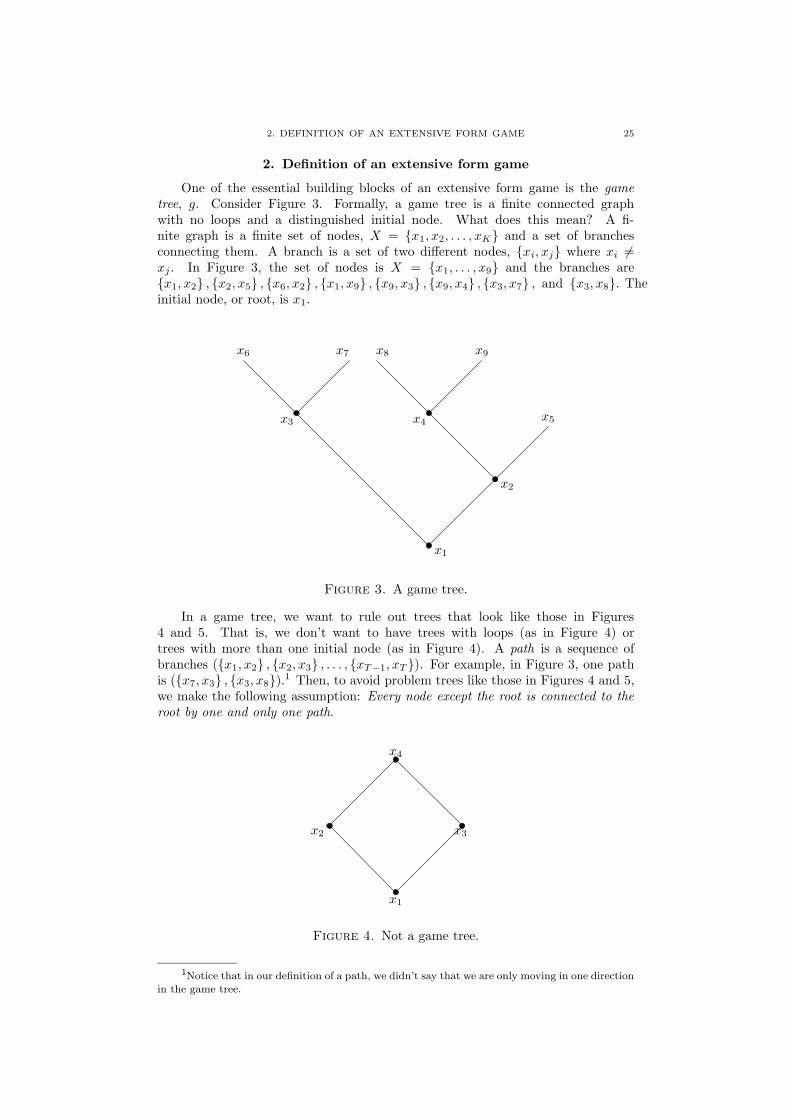
One of the essential building blocks of an extensive form game is the gametree, g. Consider Figure 3. Formally, a game tree is a finite connected graphwith no loops and a distinguished initial node. What does this mean? A fi-nite graph is a finite set of nodes, X = {x1, x2, . . . , xK} and a set of branchesconnecting them. A branch is a set of two different nodes, {xi, xj} where xi 6=xj . In Figure 3, the set of nodes is X = {x1, . . . , x9} and the branches are{x1, x2} , {x2, x5} , {x6, x2} , {x1, x9} , {x9, x3} , {x9, x4} , {x3, x7} , and {x3, x8}. Theinitial node, or root, is x1.

x1

x2

x3 x4

x6 x7 x8 x9

x5

Figure 3. A game tree.

In a game tree, we want to rule out trees that look like those in Figures4 and 5. That is, we don’t want to have trees with loops (as in Figure 4) ortrees with more than one initial node (as in Figure 4). A path is a sequence ofbranches ({x1, x2} , {x2, x3} , . . . , {xT−1, xT }). For example, in Figure 3, one pathis ({x7, x3} , {x3, x8}).1 Then, to avoid problem trees like those in Figures 4 and 5,we make the following assumption: Every node except the root is connected to theroot by one and only one path.

x1

x2 x3

x4

Figure 4. Not a game tree.

1Notice that in our definition of a path, we didn’t say that we are only moving in one direction

in the game tree.


x1 x2

x3 x4

Figure 5. Not a game tree either.

As an alternative way of avoiding game trees like those in Figures 4 and 5,given a finite set of nodes X, we define the immediate predecessor function p :X → X ∪ {∅}, to be the function that gives the node that comes immediatelybefore any given node in the game tree. For example, in Figure 3, p (x2) = x1,p (x3) = x9, p (x7) = x3, and so on. To make sure that a game tree has only oneinitial node, we require that there is a unique x0 ∈ X such that p (x0) = ∅, that is,that there is only one node with no immediate predecessor. To prevent loops in thegame tree, we require that for every x 6= x0, either p (x) = x0 or p (p (x)) = x0 or. . . p (p (p . . . p (x))) = x0. That is, by applying the immediate predecessor functionp to any node except for the initial node, eventually we get to the initial node x0.

The terminal nodes in Figure 3 are x5, x6, x7, x8, and x9. We denote theset of terminal nodes by T . A terminal node is a node such that there is a path({x0, x1} , {x1, x2} , . . . , {xt−1, xt}) and there are no paths that extend this. Alter-natively, we can say that xt is a terminal node if there is no node y ∈ X withp (y) = xt.

Now we can give a formal definition of an extensive form game.

Definition 2.1. An extensive form game consists of:

(1) N = {1, 2, . . . , N} a finite set of players.(2) X a set of nodes.(3) X is a game tree.(4) A set of actions, A, and a labelling function α : X\ {x0} → A where α (x)

is the action at the predecessor of x that leads to x. If p (x) = p (x′) andx 6= x′ then α (x) 6= α (x′).

(5) H a collection of information sets and H : X\T → H a function thatassigns for every node, except the terminal ones, which information setthe node is in.

(6) A function n : H → N ∪ {0}, where player 0 denotes Nature. Thatis, n (H) is the player who moves at information set H. Let Hn ={H ∈ H|n (H) = n} be the information sets controlled by player n.

(7) ρ : H0 × A → [0, 1] giving the probability that action a is taken at theinformation set H of Nature. That is, ρ (H, a).

(8) (u1, . . . , uN ) with un : T → R being the payoff to player n.

This completes the definition of an extensive form game. Just a few morecomments are in order at this stage.

First, let C (x) = {a ∈ A|a = αx′ for some x′ with p (x′) = x}. That is, C (x)is the set of choices that are available at node x. Note that if x is a terminal nodethen C (x) = ∅. If two nodes x and x′ are in the same information set, that is,

3. PERFECT RECALL 27

if H (x) = H (x′), then the same choices must be available at x and x′, that is,C (x) = C (x′).

To illustrate this, consider the “game” shown in Figure 6. This figure illustratesthe “forgetful driver”: A student is driving home after spending the evening at apub. He reaches a set of traffic lights and can choose to go left or right. If hegoes left, he falls off a cliff. If he goes right, he reaches another set of traffic lights.However when he gets to this second set of traffic lights, since he’s had a few drinksthis evening, he cannot remember if he passed a set of traffic lights already or not.At the second traffic lights he can again either go left or right. If he goes left he getshome and if he goes right he reaches a rooming house. The fact that he forgets atthe second set of traffic lights whether he’s already passed the first set is indicatedin Figure 6 by the nodes x0 and x1 being in the same information set. That is,H (x0) = H (x1). Under our definition, this is not a proper extensive form game.Under our definition, if two nodes are in the same information set, neither shouldbe a predecessor of the other.

x0

x1

L R

L R

Cliff

HomeRooming

House

Figure 6. The forgetful driver.

Finally, we’ll assume that all H ∈ H0 are singletons, that is, sets consisting ofonly one element. In other words, if H ∈ H0 and H (x) = H (x′) then x = x′. Thissays that Nature’s information sets always have only one node in them.

3. Perfect recall

An informal definition is that a player has perfect recall if he remembers ev-erything that he knew and everything that he did in the past. This has a fewimplications:

• If the player has only one information set then the player has perfect recall(because he has no past!).

• If it is never the case that two different information sets of the player bothoccur in a single play of the game then the player has perfect recall.

• If every information set is a single node we say the game has perfectinformation. In this case a player when called upon to move sees exactlywhat has happened in the past. If the game has perfect information theneach player has perfect recall.


Now let us give a formal definition of perfect recall. We define it in terms ofa player, and if every player in the game has perfect recall, we say that the gameitself has perfect recall.

Definition 2.2. Given an extensive form game, we say that player n in thatgame has perfect recall if whenever H (x) = H (x′) ∈ Hn, that is, whenever x andx′ are in the same information set and player n moves at that information set, withx′′ a predecessor of x with H (x′′) ∈ Hn, that is, x′′ comes before x and playern moves at x′′, and a′′ is the action at x′′ on the path to x, then there is somex′′′ ∈ H (x′′) a predecessor of x′ with a′′ the action at x′′′ on the path to x′.

4. Equilibria of extensive form games

To find the Nash equilibria of an extensive form game, we have two choices.First, we could find the equivalent normal form game and find all the equilibriafrom that game, using the methods that we learned in the previous section. Theonly trouble with this is that two different extensive form games can give the samenormal form. Alternatively, we can find the equilibria directly from the extensiveform using a concept (to be explained in subsection 9 below) called subgame perfectequilibrium (SPE). Note that we cannot find the SPE of an extensive form gamefrom its associated normal form; we must find it directly from the extensive form.The two approaches that we can take to finding the equilibria of an extensive formgame are shown in Figure 7.

Extensiveform

games

Normalform

gamesSolutions

-1 1�

*

Normal formfunction

Equilibriumcorrespondence

Subgame PerfectEquilibrium correspondence

Figure 7. Methods for defining equilibria of extensive formgames. Note that two different extensive form games may havethe same normal form and that a single game may have multipleequilibria, some of which may be subgame perfect and some ofwhich may not.

5. The associated normal form

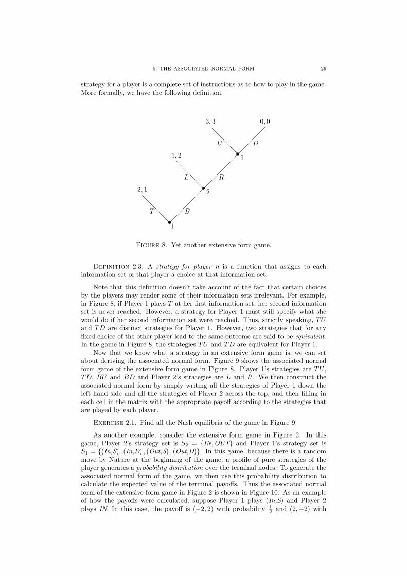
Let us first consider the method for finding equilibria of extensive form gameswhereby we find the Nash equilibria of the associated normal form. Consider theextensive form game shown in Figure 8. To find the associated normal form of thisgame, we first need to know what a strategy of a player is. As we said before, a

5. THE ASSOCIATED NORMAL FORM 29

strategy for a player is a complete set of instructions as to how to play in the game.More formally, we have the following definition.

1

2

1

T B

L R

U D

2, 1

1, 2

3, 3 0, 0

Figure 8. Yet another extensive form game.

Definition 2.3. A strategy for player n is a function that assigns to eachinformation set of that player a choice at that information set.

Note that this definition doesn’t take account of the fact that certain choicesby the players may render some of their information sets irrelevant. For example,in Figure 8, if Player 1 plays T at her first information set, her second informationset is never reached. However, a strategy for Player 1 must still specify what shewould do if her second information set were reached. Thus, strictly speaking, TUand TD are distinct strategies for Player 1. However, two strategies that for anyfixed choice of the other player lead to the same outcome are said to be equivalent.In the game in Figure 8, the strategies TU and TD are equivalent for Player 1.

Now that we know what a strategy in an extensive form game is, we can setabout deriving the associated normal form. Figure 9 shows the associated normalform game of the extensive form game in Figure 8. Player 1’s strategies are TU ,TD, BU and BD and Player 2’s strategies are L and R. We then construct theassociated normal form by simply writing all the strategies of Player 1 down theleft hand side and all the strategies of Player 2 across the top, and then filling ineach cell in the matrix with the appropriate payoff according to the strategies thatare played by each player.

Exercise 2.1. Find all the Nash equilibria of the game in Figure 9.

As another example, consider the extensive form game in Figure 2. In thisgame, Player 2’s strategy set is S2 = {IN,OUT} and Player 1’s strategy set isS1 = {(In,S) , (In,D) , (Out,S) , (Out,D)}. In this game, because there is a randommove by Nature at the beginning of the game, a profile of pure strategies of theplayer generates a probability distribution over the terminal nodes. To generate theassociated normal form of the game, we then use this probability distribution tocalculate the expected value of the terminal payoffs. Thus the associated normalform of the extensive form game in Figure 2 is shown in Figure 10. As an exampleof how the payoffs were calculated, suppose Player 1 plays (In,S) and Player 2plays IN. In this case, the payoff is (−2, 2) with probability 1

2 and (2,−2) with


Player 2

L R

TU 2, 1 2, 1

Player 1 TD 2, 1 2, 1

BU 1, 2 3, 3

BD 1, 2 0, 0

Figure 9. The normal form game corresponding to the extensiveform game in Figure 8.

probability 12 . Thus the expected payoffs are 1

2 · (−2, 2) + 12 · (2,−2) = (0, 0). If

instead Player 1 plays (In,S) and Player 2 plays OUT, the expected payoffs are12 · (1,−1) + 1

2 · (2,−2) =(1 1

2 ,−1 12

). The other payoffs are calculated similarly.

Player 2

IN OUT

In, S 0, 0 32 ,− 3

2

Player 1 In,D 0, 0 − 12 ,

12

Out, S − 32 ,

32 0, 0

Out,D 12 ,− 1

2 0, 0


Let us complete this example by finding all the Nash equilibria of the nor-mal form game in Figure 10. Note that for Player 1, the strategies (In,D) and(Out, S) are strictly dominated by, for example, the strategy

(12 , 0, 0,

12

). To see

this, suppose that Player 1 plays (In,D) and Player 2 plays a mixed strategy(y, 1− y) where 0 ≤ y ≤ 1. Then Player 1’s expected payoff from (In,D) is 0 · y +(− 1

2

)· (1− y) = − 1

2 + 12y. Suppose instead that Player 1 plays the mixed strategy(

12 , 0, 0,

12

). Player 1’s expected payoff from this strategy is 1

2

(0 · y + 1 1

2 · (1− y))+

12

(12 · y + 0 · (1− y)

)= 3

4 − 12y. Since 3

4 − 12y −

(− 1

2 + 12y)

= 54 − y ≥ 0 for any

0 ≤ y ≤ 1,(

12 , 0, 0,

12

)gives Player 1 a higher expected payoff than (In,D) whatever

Player 2 does. Similar calculations show that (Out,S) is also strictly dominatedfor Player 1. Thus we know that Player 1 will never play (In,D) or (Out,S) in aNash equilibrium. This means that we can reduce the game to the one found inFigure 11.

From Figure 11, we see that the game looks rather like that of matching penniesfrom Figure 6. We know that in such a game there are no pure strategy equilibria.In fact, there is no equilibrium in which either player plays a pure strategy. Sowe only need to check for mixed strategy equilibria. Suppose that Player 1 plays(In,S) with probability x and (Out,D) with probability 1 − x, and Player 2 playsIN with probability y and OUT with probability 1− y. Then x must be such thatPlayer 2 is indifferent between IN and OUT, which implies

0 · x+(− 1

2

)· (1− x) =

(−1 1

2

)· x+ 0. (1− x)

6. BEHAVIOUR STRATEGIES 31

Player 2

IN OUT

Player 1 In, S 0, 0 32 ,− 3

2

Out,D 12 ,− 1

2 0, 0

Figure 11. The normal form game corresponding to the exten-sive form game in Figure 2, after eliminating Player 1’s strictlydominated strategies.

which implies x = 14 . Similarly, y must be such that Player 1 is indifferent between

(In,S) and (Out,D). This implies that

0 · y + 1 12 · (1− y) = 1

2 · y + 0 · (1− y)

which implies y = 34 . So, the only Nash equilibrium of the game in Figure 11, and

hence of the game in Figure 10 is{(

14 , 0, 0,

34

),(

34 ,

14

)}.

Exercise 2.2. Consider the normal form game in Figure 10 and the Nashequilibrium strategy that we have just found.

(1) If the players play their equilibrium strategies, what is the expected payoffto each player?

(2) If Player 1 plays his equilibrium strategy, what is the worst payoff thathe can get (whatever Player 2 does)?

6. Behaviour strategies

Consider the extensive form game shown in Figure 12 and its associated normalform shown in Figure 13. In this game, we need three independent numbers todescribe a mixed strategy of Player 2, i.e., (x, y, z, 1− x− y − z). Suppose thatinstead Player 2 puts off her decision about which strategy to use until she is calledupon to move. In this case we only need two independent numbers to describethe uncertainty about what Player 2 is going to do. That is, we could say that atPlayer 2’s left-hand information set she would choose L with probability x and Rwith probability 1− x, and at her right-hand information set she would choose Wwith probability y and E with probability 1 − y. We can see that by describingPlayer 2’s strategies in this way, we can save ourselves some work. This efficiencyincreases very quickly depending on the number of information sets and the numberof choices at each information set. For example, suppose that the game is similarto that of Figure 12, except that Player 1’s choice is between four strategies, eachof which leads to a choice of Player 2 between three strategies. In this case Player 2has 3·3·3·3 = 81 different pure strategies and we’d need 80 independent numbers todescribe the uncertainty about what Player 2 is going to do! If instead we supposethat Player 2 puts off her decision about which strategy to use until she is calledupon to move, we only need 4 · 2 = 8 independent numbers. This is really great!

When we say that a player “puts off” his or her decision about which strategyto use until he or she is called upon to move, what we really mean is that weare using what is called a behaviour strategy to describe what the player is doing.Formally, we have the following definition.

Definition 2.4. In a given extensive form game with player set N , a behaviourstrategy for player n ∈ N is a rule, or function, that assigns to each information set of


1

22

T B

W EL R

1, 42, 20, 03, 3


Player 2

LW LE RW RE

Player 1 T 3, 3 3, 3 0, 0 0, 0

B 2, 2 1, 4 2, 2 1, 4


that player a probability distribution over the choices available at that informationset.

7. Kuhn’s theorem

Remember we motivated behaviour strategies in subsection 6 as a way of re-ducing the amount of numbers we need compared to using mixed strategies. Youmight be wondering whether we can always do this, that is, if we can representany arbitrary mixed strategy by a behaviour strategy. The answer is provided byKuhn’s theorem.

Theorem 2.1. (Kuhn) Given an extensive form game, a player n who has per-fect recall in that game, and a mixed strategy σn of player n, there exists a behaviourstrategy bn of player n such that for any profile of strategies of the other players(x1, . . . , xn−1, xn+1, . . . , xN ) where xm, m 6= n, is either a mixed strategy of a be-haviour strategy of player m, the strategy profiles (x1, . . . , xn−1, σn, xn+1, . . . , xN )and (x1, . . . , xn−1, bn, xn+1, . . . , xN ) give the same distribution over terminal nodes.

In other words, Kuhn’s theorem says that given what the other players aredoing, we can get the same distribution over terminal nodes from σn and bn, aslong as player n has perfect recall. To see Kuhn’s theorem in action, considerthe game in Figure 14. Suppose Player 1 plays T with probability p and B withprobability 1− p. Player 2’s pure strategies are XA, XB, Y A, and Y B. SupposePlayer 2 plays a mixed strategy of playing XA and Y B with probability 1

2 and XB

and Y A with probability 0. Thus, with probability 12 , Player 2 plays XA and we

get to terminal node x with probability p and to terminal node a with probability1−p, and with probability 1

2 , Player 2 plays Y B and we get to terminal node y withprobability p and terminal node b with probability 1− p. This gives a distributionover terminal nodes as shown in the table in Figure 15.

8. MORE THAN TWO PLAYERS 33

1

22

T B

A BX Y

bayx


Terminal node Probabilityx p/2y p/2a (1− p) /2b (1− p) /2

Figure 15. Distributions over terminal nodes in the game of Fig-ure 14 for the strategy profile given in the text.

Now suppose that Player 2 plays a behaviour strategy of playing X with prob-ability 1

2 at his left-hand information set and A with probability 12 at his right-hand

information set. Thus we get to terminal node x with probability p · 12 , to terminal

node y with probability p · 12 , to terminal node a with probability (1− p) · 1

2 and

to terminal node b with probability (1− p) · 12 . Just as Kuhn’s theorem predicts,

there is a behaviour strategy that gives the same distribution over terminal nodesas the mixed strategy.

8. More than two players

1

2

3

T B

L R

U D

2, 7, 1

6, 2, 7

3, 3, 3 1, 1, 1

Figure 16. An extensive form game with three players.


It is easy to draw extensive form games that have more than two players, suchas the one shown in Figure 16, which has three players. How would we find theassociated normal form of such a game? Recall that a normal form game is givenby (N,S, u). For the game in Figure 16, we have N = {1, 2, 3}, S1 = {T,B},S2 = {L,R} and S3 = {U,D}, hence

S = {(T,L, U) , (T,L,D) , (T,R,U) , (T,R,D) , (B,L,U) , (B,L,D) ,

(B,R,U) , (B,R,D)}.Finally, the payoff functions of each player are shown in Figure 17.

S T,L, U T, L,D T,R,U T,R,D B,L,U B,L,D B,R,U B,R,Du1 2 2 2 2 6 6 3 1u2 7 7 7 7 2 2 3 1u3 1 1 1 1 7 7 3 1

Figure 17. One way of presenting the normal form game associ-ated with the extensive form game of Figure 16.

The form shown in Figure 17 is a perfectly acceptable exposition of the asso-ciated normal form. However, it’s more convenient to represent this three playergame as shown in Figure 18, where Player 3 chooses the matrix.

Player 3

U D

Player 1

Player 2

L R

T 2, 7, 1 2, 7, 1

B 6, 2, 7 3, 3, 3

Player 1

Player 2

L R

T 2, 7, 1 2, 7, 1

B 6, 2, 7 1, 1, 1

Figure 18. A more convenient representation of the normal formof the game in Figure 16.

9. Subgame perfect equilibrium

Subgame perfect equilibrium is an equilibrium concept that relates directly tothe extensive form of a game. The basic idea is that equilibrium strategies shouldcontinue to be an equilibrium in each subgame (subgames will be defined formallybelow).

Definition 2.5. A subgame perfect equilibrium is a profile of strategies suchthat for every subgame the parts of the profile relevant to the subgame constitutean equilibrium of the subgame.

To understand subgame perfect equilibrium, we first need to know what asubgame is. Consider the game in Figure 16. This game has two proper subgames.Strictly speaking, the whole game is a subgame of itself, so we call subgames thatare not the whole game proper subgames. The first is the game that begins fromPlayer 2’s decision node and the second is the game that begins from player 3’sdecision node. However, it would be a mistake to think that every game has proper

9. SUBGAME PERFECT EQUILIBRIUM 35

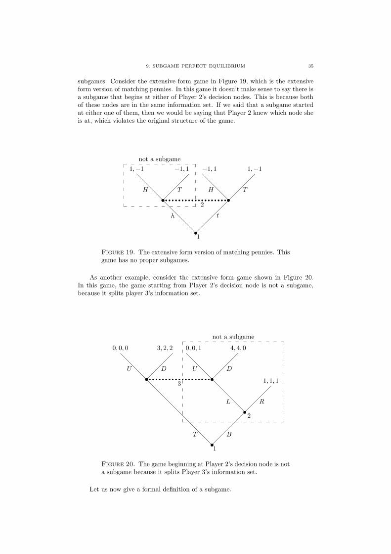
subgames. Consider the extensive form game in Figure 19, which is the extensiveform version of matching pennies. In this game it doesn’t make sense to say there isa subgame that begins at either of Player 2’s decision nodes. This is because bothof these nodes are in the same information set. If we said that a subgame startedat either one of them, then we would be saying that Player 2 knew which node sheis at, which violates the original structure of the game.

1

2

not a subgame

h t

H TH T

1,−1−1, 1−1, 11,−1

Figure 19. The extensive form version of matching pennies. Thisgame has no proper subgames.

As another example, consider the extensive form game shown in Figure 20.In this game, the game starting from Player 2’s decision node is not a subgame,because it splits player 3’s information set.

not a subgame

1

2

3

T B

L R

U DU D

0, 0, 0 3, 2, 2 0, 0, 1 4, 4, 0

1, 1, 1

Figure 20. The game beginning at Player 2’s decision node is nota subgame because it splits Player 3’s information set.

Let us now give a formal definition of a subgame.


Definition 2.6. A subgame of an extensive form game Γ is some node inthe tree of Γ and all the nodes that follow it, with the original tree structure butrestricted to this subset of nodes, with the property that any information set of Γis either completely in the subgame or completely outside the subgame. The restof the structure is the same as in Γ but restricted to the new (smaller) tree.

Notice that under this definition, Γ is a subgame of Γ. We call subgames thatare not Γ itself proper subgames of Γ.

And we are now in a position to give a more formal definition of subgameperfect equilibrium.

Definition 2.7. A subgame perfect equilibrium of an extensive form game Γwith perfect recall is a profile of behaviour strategies (b1, b2, . . . , bN ) such that, forevery subgame Γ′ of Γ, (b′1, b

′2, . . . , b

′N ) is a Nash equilibrium of Γ′ where b′n is bn

restricted to Γ′.

9.1. Finding subgame perfect equilibria. An example of the simplest typeof extensive form game in which subgame perfect equilibrium is interesting is shownin Figure 21. Notice that in this game, (T,R) is a Nash equilibrium (of the wholegame). Given that Player 1 plays T , Player 2 is indifferent between L and R. Andgiven that Player 2 plays R, Player 1 prefers to play T . There is something strangeabout this equilibrium, however. Surely, if Player 2 was actually called upon tomove, she would play L rather than R. The idea of subgame perfect equilibrium isto get rid of this silly type of Nash equilibrium. In a subgame perfect equilibrium,Player 2 should behave rationally if her information set is reached. Thus Player 2playing R cannot form part of a subgame perfect equilibrium. Rather, if Player 2 iscalled upon to move, the only rational thing for her to do is to play L. This meansthat Player 1 will prefer B over T , and the only subgame perfect equilibrium ofthis game is (B,L). Note that (B,L) is also a Nash equilibrium of the whole game.This is true in general: Subgame perfect equilibria are always Nash equilibria, butNash equilibria are not necessarily subgame perfect.

1

2

T B

L R

1, 1

2, 2 0, 0

Figure 21. An example of the simplest type of game in whichsubgame perfect equilibrium is interesting.

As another example, consider the extensive form game in Figure 22. In thisgame, players 1 and 2 are playing a prisoners’ dilemma, while at the beginning ofthe game player 3 gets to choose whether players 1 and 2 will actually play theprisoners’ dilemma or whether the game will end. The only proper subgame of thisgame begins at Player 1’s node. We claim that (C,C,L) is a Nash equilibrium ofthe whole game. Given that player 3 is playing L, players 1 and 2 can do whateverthey like without affecting their payoffs and do not care what the other is playing.

10. SEQUENTIAL EQUILIBRIUM 37

And given that players 1 and 2 are both playing C, player 3 does best by playingL. However, although (C,C,L) is a Nash equilibrium of the game, it is not asubgame perfect equilibrium. This is because (C,C) is not a Nash equilibrium ofthe subgame beginning at Player 1’s decision node. Given that Player 1 is playingC, Player 2 would be better off playing D, and similarly for Player 1. The onlysubgame perfect equilibrium is (D,D,A).

3

1

2

L A

C D

C DC D

10, 10, 1

1, 1, 1010, 0, 100, 10, 109, 9, 0

Figure 22. Player 3 chooses whether or not Players 1 and 2 willplay a prisoners’ dilemma game.

In the previous example, we have seen that a extensive form games can haveequilibria that are Nash but not subgame perfect. You might then be wonderingwhether it’s possible to have an extensive form game that has no subgame perfectequilibria. The answer is no. Selten in 1965 proved that every finite extensive formgame with perfect recall has at least one subgame perfect equilibrium.

9.2. Backwards induction. Backwards induction is a convenient way of find-ing subgame perfect equilibria of extensive form games. We simply proceed back-wards through the game tree, starting from the subgames that have no propersubgames of themselves, and pick an equilibrium. We then replace the subgame bya terminal node with payoff equal to the expected payoff in the equilibrium of thesubgame. Then repeat, as necessary.

As an illustration, consider the game in Figure 23. First Player 1 moves andchooses whether she and Player 2 will play a battle of the sexes game or a coordi-nation game. There are two proper subgames of this game, the battle of the sexessubgame and the coordination subgame. Following the backwards induction pro-cedure, one possible equilibrium of the battle of the sexes subgame is (F, F ), andone possible equilibrium of the coordination subgame is (B, b). We then replaceeach subgame by the appropriate expected payoffs, as shown in Figure 24. We canthen see that at the initial node, Player 1 will choose S. Thus one subgame perfectequilibrium of this game is ((S, F,B) , (F, b)).

10. Sequential equilibrium

Consider the game shown in Figure 25. This game is known as “Selten’s Horse”.In this game, there are no proper subgames, hence all Nash equilibria are subgameperfect. Note that (T,R,D) is a Nash equilibrium (and hence subgame perfect).But in this equilibrium, Player 2 isn’t really being rational, because if player 3 is


1

S C

1

2

F B

F BF B

1, 30, 00, 03, 1

1

2

A B

a ba b

1, 10, 00, 04, 4

Figure 23. Player 1 chooses battle of the sexes or coordinationgame.

1

S C

3, 1 1, 1

Figure 24. Replacing the subgames with the equilibrium ex-pected payoff in each subgame.

really playing D then if Player 2 actually got to move, she would be better offplaying L rather R. Thus we have another “silly” Nash equilibrium, and subgameperfection is no help to us here to eliminate it. This kind of game lead to thedevelopment of another equilibrium concept called sequential equilibrium.

1

2

3

T B

L R

U DU D

0, 0, 0 3, 2, 2 0, 0, 1 4, 4, 0

1, 1, 1

Figure 25. “Selten’s Horse”.

Exercise 2.3. Find all the Nash equilibria of the game in Figure 25.

A sequential equilibrium is a pair, (b, µ) where b is a profile of behaviour strate-gies and µ is a system of beliefs. That is, µ is a profile of probability distributions,one for each information set, over the nodes in the information set. The system of

10. SEQUENTIAL EQUILIBRIUM 39

beliefs summarises the probabilities with which each player believes he is at eachof the nodes within each of his information sets.

To be a sequential equilibrium, the pair (b, µ) must satisfy two properties:

(1) At each information set, b puts positive weight only on those actions thatare optimal given b and µ. This is called sequential rationality.

(2) µ and b should be consistent. This means that if anything can be inferredabout µ from b then µ should be that.

If we drop the consistency requirement, we get another equilibrium conceptcalled Perfect Bayesian Equilibrium, which we won’t talk about in this course butyou might come across in other books.

Nature

2

1

12

12

IN OUTINOUT

L R L R

−2, 2 2,−2 2,−2 −2, 2

−1, 11,−1

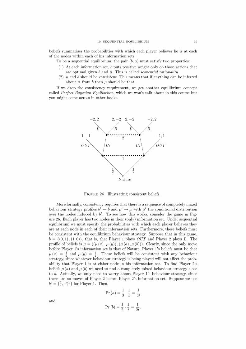
Figure 26. Illustrating consistent beliefs.

More formally, consistency requires that there is a sequence of completely mixedbehaviour strategy profiles bt → b and µt → µ with µt the conditional distributionover the nodes induced by bt. To see how this works, consider the game in Fig-ure 26. Each player has two nodes in their (only) information set. Under sequentialequilibrium we must specify the probabilities with which each player believes theyare at each node in each of their information sets. Furthermore, these beliefs mustbe consistent with the equilibrium behaviour strategy. Suppose that in this game,b = {(0, 1) , (1, 0)}, that is, that Player 1 plays OUT and Player 2 plays L. Theprofile of beliefs is µ = ((µ (x) , µ (y)) , (µ (a) , µ (b))). Clearly, since the only movebefore Player 1’s information set is that of Nature, Player 1’s beliefs must be thatµ (x) = 1

2 and µ (y) = 12 . These beliefs will be consistent with any behaviour

strategy, since whatever behaviour strategy is being played will not affect the prob-ability that Player 1 is at either node in his information set. To find Player 2’sbeliefs µ (a) and µ (b) we need to find a completely mixed behaviour strategy closeto b. Actually, we only need to worry about Player 1’s behaviour strategy, sincethere are no moves of Player 2 before Player 2’s information set. Suppose we usebt =

(1t ,t−1t

)for Player 1. Then,

Pr (a) =1

2· 1

t=

1

2t

and

Pr (b) =1

2· 1

t=

1

2t.


Thus,

µt (a) =12t

12t + 1

2t

=1

2.

Similarly, we can show that µt (b) = 12 also.

Why couldn’t we just use Player 1’s behaviour strategy (0, 1)? Because in thiscase Player 1 plays OUT and thus Player 2’s information set is not reached. Math-ematically, we would have

µ (a) =12 · 0

12 · 0 + 1

2 · 0which is not defined. So we must use completely mixed behaviour strategies closeto b to find the (consistent) beliefs, since if we use a completely mixed behaviourstrategy, every information set in the game will be reached with strictly positiveprobability (even if the probability is very small).

11. Signaling games

Signaling games are a special type of extensive form game that arise in manyeconomic models. The basic structure of a signaling game is as follows:

(1) Nature moves first, and picks one “state of nature” or “type of Player 1”.(2) Player 1 sees the result of Nature’s move, and makes his choice. It is as-

sumed that Player 1’s available actions do not depend on Nature’s choice.(3) Player 2 sees Player 1’s choice but not Nature’s, and makes her choice.(4) Payoffs are determined based on the choices of the two players and Nature,

and the game ends.

The extensive form of a simple signaling game is shown in Figure 27. In thisgame, Player 1 is either type a or b with probability 1

2 . Player 1 can choose T or B.Player 2 then observes Player 1’s choice but not Nature’s choice. If Player 1 choseT then Player 2 chooses between L and R and if Player 1 chose B then Player 2chooses between X, Y , and Z (this illustrates the fact that Player 2’s availablechoices can depend on Player 1’s choice, but neither player’s available choices candepend on Nature’s choice).

Nature

2 2

1 1

12

12

T BBT

X Y ZX Y ZL R

L R

2, 2 3, 3 2, 2 2, 2 2, 21, 01, 11, 10, 01, 1

Figure 27. The extensive form of a simple signaling game.

11. SIGNALING GAMES 41

Typically, signaling games are not presented in the form of Figure 27, however.Instead, a presentation due originally to Kreps and Wilson (1982) is used, in whichwe suppress Nature’s move and instead have a number of initial nodes with associ-ated probabilities. This alternative presentation of the game in Figure 27 is shownin Figure 28. As you can see, it is much neater to present signaling games in thisway.

T B

X

Y

Z

L

R

T B

X

Y

Z

L

R

[ 12 ]

[ 12 ]

1b

1a

22

3, 2

0, 1

0, 0

3, 0

0, 0

0, 1

4, 3

2, 2

2, 0

1, 2

Figure 28. An alternative, and tidier, presentation of the exten-sive form signaling game in Figure 27.

One economic example of a signaling game is as follows. In some market thereis an incumbent firm that sets its price in the time period before a potential entrantenters the market. The incumbent knows if the market demand conditions are goodor bad. The potential entrant does not know the demand conditions but does seethe price chosen by the incumbent. The entrant then decides whether to enter ornot. If the entrant enters, it finds out the market conditions and then there issome competition in the second period. The fixed costs are such that the entrantwill make positive profits only if market conditions are good. A representation ofthis game is shown in Figure 29, where it is assumed that the incumbent can onlychoose a ‘high’ or ‘low’ price.

L H

E

S

E

S

L H

E

S

E

S

[pB ]

[pG]

1B

1G

22

3, 1

10, 0

1,−1

3, 0

2, 1

9, 0

2,−1

4, 0

Figure 29. A simple price signaling game.

A famous signaling game is shown in Figure 30. The story behind this game isas follows. There are two players, Player A and Player B. At the beginning of thegame, Nature selects Player A to be either a wimp (with probability 0.1) or surly(with probability 0.9). At the start of the game, Player A knows whether he is awimp or surly. Player A then has to choose what to have for breakfast. He has


two choices: beer or quiche.2 If Player A is surly, he prefers beer for breakfast andif Player A is a wimp he prefers quiche for breakfast, everything else equal. Thatis, if Player A has his preferred breakfast, his incremental payoff is 1, otherwise0. After breakfast, Player A meets Player B. At the meeting, Player B observeswhat Player A had for breakfast (perhaps by seeing the bits of quiche stuck inPlayer A’s beard if Player A had quiche for breakfast or smelling the alcohol onPlayer A’s breath if A had beer for breakfast), but Player B does not know whetherPlayer A is a wimp or surly. Having observed Player A’s breakfast, Player B mustthen choose whether or not to duel (fight) with Player A. Then the game ends andpayoffs are decided. Regardless of whether Player A is a wimp or surly, Player Adislikes fighting. Thus Player A’s incremental payoff is 2 if Player B chooses not toduel and 0 if Player B chooses to duel. So, for example, if Player A is surly and hashis preferred breakfast of beer and then Player B chooses not to duel, Player A’spayoff is 1 + 2 = 3. Or, if Player A is a wimp and has his less preferred breakfastof beer and Player B chooses to duel, Player A’s payoff is 0 + 0 = 0. Player B, onthe other hand, only prefers to duel if Player A is a wimp. If Player A is surly andPlayer B chooses to duel, Player B’s payoff is 0, while if Player B chooses not toduel Player B’s payoff is 1. If Player A is a wimp and Player B chooses to duel,Player B’s payoff is 2, while if Player B chooses not to duel his payoff is 1.3

don’tduel

duel

don’tduel

duel

don’tduel

duel

don’tduel

duel

beer quiche

beer quiche

[.1]

[.9]

AW

AS

BQBB

2, 1

0, 0

3, 1

1, 2

3, 1

1, 0

2, 1

0, 2

Figure 30. The beer quiche game of Cho and Kreps.

Exercise 2.4. Consider the signaling game in Figure 30.

(1) Find the normal form of this game.(2) Find all the pure strategy Nash equilibria (from the normal form).(3) Find all the mixed strategy Nash equilibria (from the normal form).

Since the beer-quiche game in Figure 30 is a game of asymmetric information(that is, Player B doesn’t know whether Player A is surly or a wimp), it makes senseto look for a sequential equilibrium. In this game a sequential equilibrium will bean assessment ((bA, bB) , µ) that is consistent and sequentially rational, where

bA = ((bAS (beer) , bAS (quiche)) , (bAW (beer) , bAW (quiche)))

bB = ((bBB (don’t) , bBB (duel)) , bBQ (don’t) , bBQ (duel))

µ = ((µbeer (S) , µbeer (W )) , (µquiche (S) , µquiche (W ))) .

2For those of you who don’t know, quiche is a sort-of egg pie type thing that only wimps and

Australian rugby players eat.3Note that Player B’s payoff only depends on his own decision about whether to duel or not,

and whether Player A is surly or a wimp. That is, Player B’s payoff does not depend on whatPlayer A had for breakfast.

11. SIGNALING GAMES 43

In such a game as this, there are two basic types of equilibrium that can arise. Inthe first type of equilibrium, called a pooling equilibrium, both types of Player Achoose the same probabilities for having beer and quiche for breakfast. In this case,Player A’s breakfast gives Player B no information about Player A’s type and thusPlayer B’s best estimate of Player A’s type is that Player A is surly with probability0.9 and a wimp with probability 0.1. In the second type of equilibrium, called aseparating equilibrium, the two types of Player A choose different probabilities forthe breakfasts. In this case, Player B gets some information about Player A’s typefrom Player A’s breakfast, and will be able to modify his estimate of Player A’stype.

You will analyse this game more fully in tutorials. So as not to spoil the fun,we shall content ourselves with just answering one question about this game here:Are there any equilibria in which both beer and quiche are played with positiveprobability? Before answering this question, note the following facts about thegame:

(1) If bB is such that the surly Player A is willing to have quiche for breakfastthen the wimp Player A strictly wants to have quiche for breakfast (sincequiche is the wimp’s preferred breakfast).

(2) Similarly, if bB is such that the wimp Player A wants to have beer forbreakfast then the surly Player A strictly wants to have beer for breakfast.

Now suppose that in equilibrium the surly pPlayer A plays quiche with positiveprobability. Then by fact (1), the wimp Player A plays quiche with probability 1.Thus either surly Player A plays quiche with probability 1, in which case beer isnot played with positive probability, or surly Player A plays beer with positiveprobability. But then µbeer (S) = 1 and thus Player B chooses not to duel afterobserving Player A having beer for breakfast, that is, bBB (duel) = 0. But thensurly Player A will not want to play quiche with positive probability.

Suppose, on the other hand, that surly Player A plays beer with probability1, i.e., bAS (beer) = 1. Then µbeer (S) ≥ 0.9. Then sequential rationality impliesbBB ( duel) = 0. So if wimp Player A plays quiche with positive probability thenµquiche (S) = 0 and µquiche (W ) = 1 and so bBQ (duel) = 1. Thus wimp Player Achooses beer for sure and quiche is not played with positive probability.

So, we have established that there are no sequential equilibria in which bothbeer and quiche are played with strictly positive probability. As you will discover intutorials, there are sequential equilibria in which both types of Player A play beerand there are sequential equilibria in which both types of Player A play quiche.

Extensive Form Games - College of Arts and Sciences

Documents

Transcript of Extensive Form Games - College of Arts and Sciences