Extending the LTE-Sim for LTE-Advance with CoMP … Thesis... · i University of Technology, Sydney...

i

University of Technology, Sydney

Faculty of Engineering and Information Technology

Extending the LTE-Sim for LTE-Advance with CoMP and Relaying in Heterogeneous 4G

Mobile Networks

Haider Al Kim 11569249

Supervisor: Associate Professor Kumbesan Sandrasegaran

The work contained in this report, other than that specifically attributed to another

source, is that of the author(s). It is recognised that, should this declaration be found to

be false, disciplinary action could be taken and the assignments of all students involved

will be given zero marks.

Signed:

Date: 21/11/2014

i

Acknowledgement

First of all, I would like to express my warm thanks to Imam Sahib Al Zaman

(as) who is always a beacon shining on my way to success.

This master thesis project is the final stage in obtaining the master degree in

telecommunication networks at the University of Technology Sydney (UTS). This

project was conducted in the Centre for Real-Time Information Networks (CRIN) in the

faculty of engineering and information technology in the UTS. I have been working in

this project from March 2014 to November 2014. During this project I have had much

support from several people. I would like to express my honest gratitude below.

Associate Professor Kumbesan Sandrasegaran has been my supervisor for this project.

He was been a great support providing guidance, advice, constructive criticism and

encouragement over the course of the last year. In addition, I am deeply and forever

indebted to my parents. My sincere appreciation and gratitude to them is for their efforts

and their distinctive role in all fields of my life, besides their faith in me and allowing

me to be as ambitious as I wanted. Your prayer for me was what sustained me thus far.

Importantly, my grateful thanks are extended to my wife, Ruwaida. Her support,

encouragement, quiet patience and unwavering love were undeniably the bedrock upon

which the past five years of my life have been built. Warm thanks for my brothers and

sisters for their unwavering supports.

Finally, for all of these people who motivated me to do the best and were

confident that I will be the best, I offer this modest gift to express thanks.

ii

Acknowledgement....................................................................................................................... i

Contents ..................................................................................................................................... ii

List of Figures ........................................................................................................................... iv

List of Tables.............................................................................................................................. v

Abbreviation List ...................................................................................................................... vi

Abstract ...................................................................................................................................... x

1. Chapter 1: Introduction ...................................................................................................... 1

1.1. Background 1

1.2. Motivation and goal of the project ...................................................................................... 3

1.2.1. Motivation ........................................................................................................................ 3

1.2.2. Thesis objective ................................................................................................................ 3

1.2.3. Thesis Scope .................................................................................................................... 3

2. Chapter 2: LTE-A ............................................................................................................... 4

2.1. Introduction 4

2.2. LTE- Advance Enhancements............................................................................................. 5

2.2.1. Air Interface Enhancement .............................................................................................. 5

2.2.1.1. Channel Bandwidth Structure ....................................................................................... 5

2.2.1.2. Carrier Aggregation ...................................................................................................... 6

2.2.1.3. Effective and Guard bands ............................................................................................ 9

2.2.2. Improving spectral efficiency ........................................................................................ 10

2.2.2.1. Heterogeneous Network (HetNets) ............................................................................. 11

2.2.2.2. HetNets Challenges ..................................................................................................... 14

2.2.2.3. Higher Spectrum Utilization. ...................................................................................... 15

2.2.3. Signaling Optimizations ................................................................................................. 15

2.2.3.1. Frequency Domain ICIC: ............................................................................................ 15

2.2.3.2. Time Domain ICIC ..................................................................................................... 16

2.2.4. Network Based Techniques............................................................................................ 19

2.2.4.1. Advanced MIMO Scheme .......................................................................................... 19

2.2.4.2. Transmission/Reception Coordinated Multi-Point ..................................................... 21

2.2.4.3. Relays .......................................................................................................................... 24

2.3. Summary 32

3. Chapter 3: Radio Resource Management ...................................................................... 34

3.1. Introduction 34

3.2. RRM in both DL and UL .................................................................................................. 35

3.2.1. Connection Mobility Control (CMC)............................................................................. 35

3.2.1.1. Handover ..................................................................................................................... 36

3.2.1.2. Future Trends of Handover ......................................................................................... 40

3.2.1.3. Handover Phases in LTE-A ........................................................................................ 40

3.2.2. Admission Control ......................................................................................................... 47

3.2.3. Packet Scheduling (PS) .................................................................................................. 49

3.2.3.1. Downlink Packet Scheduling ...................................................................................... 51

3.2.3.2. Packet Scheduling Algorithms in Downlink Direction ............................................... 53

3.2.3.3. Uplink Packet Scheduling ........................................................................................... 57

3.2.4. Power Control (PC) ........................................................................................................ 58

iii

3.2.5. Balancing of Carrier Load .............................................................................................. 60

3.2.5.1. Carrier Load Balancing ............................................................................................... 60

3.2.6. Interference Management............................................................................................... 61

3.3. Summary 62

4. Chapter 4: LTE-Sim Heterogeneous Network Deployment .......................................... 65

4.1. Introduction 65

4.2. Downlink System Model of LTE ...................................................................................... 66

4.3. Packet Scheduling Algorithms .......................................................................................... 68

4.3.1. Proportional Fair (PF) Algorithm................................................................................... 68

4.3.2. Maximum Largest Weighted Delay First (MLWDF) Algorithm .................................. 69

4.3.3. Exponential/Proportional Fair (EXP/PF) Algorithm ..................................................... 70

4.4. Simulation.1- Single Macro Cell with two Pico Cells ...................................................... 70

4.4.1. Simulation.1 Environment ............................................................................................. 71

4.4.2. Simulation.1 Results ...................................................................................................... 74

4.4.2.1. Throughput .................................................................................................................. 74

4.4.2.2. Packet Loss Ratio (PLR) ............................................................................................. 75

4.4.2.3. Delay ........................................................................................................................... 76

4.4.2.4. Fairness Index ............................................................................................................. 77

4.5. Simulation.2-Single Macro Cell with two Pico Cells (Different Speed Comparison) ..... 78



4.5.2.1. Throughput .................................................................................................................. 79


4.5.2.3. Delay ........................................................................................................................... 81

4.5.2.4. Fairness Index ............................................................................................................. 81

4.6. Simulation.3- Single Macro Cell with Increasing Pico Cells ........................................... 82



4.6.2.1. Throughput .................................................................................................................. 84


4.6.2.3. Delay ........................................................................................................................... 88

4.6.2.4. Fairness Index ............................................................................................................. 90

4.7. Conclusion 91

iv

List of Figures

Figure 2.1 Evolution of LTE-Advance ..................................................................................... 4

Figure 2.2 Carrier Aggregation .................................................................................................. 7

Figure 2.3 LTE-A Protocols Stack ............................................................................................. 8

Figure 2.4 Aggregation Process ................................................................................................. 9

Figure 2.5 Effective and Guard Bands with Aggregation Calculations .................................. 10

Figure 2.6 Heterogeneous Network Example .......................................................................... 11

Figure 2.7 Driving Factors and enablers for small cell deployment ....................................... 12

Figure 2.8 Main Comparison between HetNets layers, MLC (Minimum Coupling Loss) .... 13

Figure 2.9 Small Cell Extension concepts Usage to Offload Macro Cell ................................ 14

Figure 2.10 CA-based ICIC in HetNets .................................................................................... 16

Figure 2.11 ABS concept to provide interference free in HetNets ........................................... 17

Figure 2.12 Flowchart indicate ABS information elements exchange over X2 ........................ 18

Figure 2.13 SU-MIMO and MU-MIMO .................................................................................... 19

Figure 2.14 Advanced MIMO .................................................................................................... 20

Figure 2.15 Coordinated Scheduling/Beamforming .................................................................. 21

Figure 2.16 Joint Processing [28]............................................................................................... 23

Figure 2.17 Uplink Coordinated Scheduling ............................................................................. 23

Figure 2.18 Relays Node (RN) architecture ............................................................................... 25

Figure 2.19 Relays Duplexing Schemes .................................................................................... 27

Figure 2.20 FDD/TDD relay system .......................................................................................... 28

Figure 2.21 A repeater protocol stack (layer 1 performing relaying) ........................................ 29

Figure 2.22 Layer 2 Protocol Stack (Decoding/Encoding) ........................................................ 30

Figure 2.24 Protocol stack of RN ............................................................................................... 31

Figure 2.23 Protocol stack (Layer 3).......................................................................................... 31

Figure 3.1 RRM functions and the mapping to the lower layers ............................................. 34

Figure 3.2 Principle of Macro Diversity Handover ................................................................. 37

Figure 3.3 Principle of Fast Base Station Switching Handover ............................................... 37

Figure 3.4 Hard Handover ....................................................................................................... 38

Figure 3.5 Multicarrier Handover ............................................................................................ 39

Figure 3.6 X2 Initiation Phase [34] .......................................................................................... 41

Figure 3.7 X2 based Handover –Preparation Phases ............................................................... 42

Figure 3.8 S1 based Handover – Preparation Phases ............................................................... 43

Figure 3.9 Handover Execution Phase ..................................................................................... 45

Figure 3.10 Handover Completion Phase-X1 based Handover ................................................. 46

Figure 3.11 Handover Completion Phase-S1 based Handover .................................................. 47

Figure 3.12 RRM Framework in LTE-A ................................................................................... 50

Figure 3.13 Interactions between HARQ, PS and LA ............................................................... 52

Figure 3.14 Frequency DPS Concept ........................................................................................ 52

Figure 3.15 Uplink RRM Functionalities inter-work with LA and PS ..................................... 58

Figure 3.16 eNB Classification for LTE Rel 8 and LTE-A Arrival UEs .................................. 60

Figure 4.1 An Example of HetNets .......................................................................................... 65

Figure 4.2 Downlink Packet Scheduler of the 3GPP LTE System .......................................... 68

Figure 4.3 Applied HetNets (Macro with 2 Picos) .................................................................. 72

Figure 4.4 Average System Throughput (Macro with 2 Picos) ............................................... 74

Figure 4.5 Average System Throughput (single Macro cell) ................................................... 75

Figure 4.6 PLR of Video Flows (single Macro cell) ................................................................ 75

Figure 4.7 PLR of Video Flows (Macro with 2 Picos) ............................................................ 76

Figure 4.8 Packet Delay of Video Flows (single Macro cell) .................................................. 77

v

Figure 4.9 Packet Delay of Video Flows (Macro with 2 Picos) .............................................. 77

Figure 4.10 Fairness Index of Video Flows [15] ....................................................................... 78

Figure 4.11 Fairness Index of Video Flows Macro with 2 Picos ............................................... 78

Figure 4.12 Throughput of Video in Macro with 2 Picos ........................................................... 80

Figure 4.13 PLR of Video in Macro with 2 Picos (3 Km/h and 120 Km/h speed) ..................... 80

Figure 4.14 Delay of Video in Macro with 2 Picos (3 Km/h and 120 Km/h speed)................... 81

Figure 4.15 Fairness Index in Macro with 2 Picos (3 Km/h and 120 Km/h speed) .................... 82

Figure 4. 16 Applied HetNets (Macro with Multiple Picos Scenarios) ...................................... 83

Figure 4.17 Throughput Gain of Video traffic in Macro with 2-10 Picos Scenarios .................. 85

Figure 4.18 Throughput Gain of Video traffic in Macro with 2-10 Picos Scenarios .................. 86

Figure 4.19 PLR Video traffic Comparison in Macro with 2-10 Picos Scenarios ...................... 87

Figure 4.20 PLR of Video traffic in Macro with 2-10 Picos Scenarios ...................................... 87

Figure 4.21 Delay of Video traffic Comparison in Macro with 2-10 Picos Scenarios ............... 89

Figure 4.22 Comparison Delay of Video traffic in Macro with 2-10 Picos Scenarios ............... 89

Figure 4.23 Fairness Index in Macro with 2-10 Picos Scenarios ................................................ 90

Figure 4.24 Fairness Index in Macro with 2-10 Picos Scenarios ................................................ 91

List of Tables

Table 2.1 LTE-A agreed requirements.......................................................................................... 5

Table 2.2 Carrier Aggregation Models ......................................................................................... 7

Table 3.1 QCI Parameters for EPS Bearer QoS Profile .............................................................. 48

Table 4.1 Mapping between instantaneous downlink SNR and data rate ................................... 67

Table 4.2 LTE System Simulation Parameters ........................................................................... 73

Table 4.3 Pico Cells Positions in meters into the Macro Cell (Radius 1 Km) ............................ 83

Table 4.4 Throughput Gain Values and An Average of The Values .......................................... 85

Table 4.5 PF Throughput Gain Values and An Average of The Values..................................... 88

vi

Abbreviation List

1G First Generation

2G Second Generation

3G Third Generation

4G Fourth Generation

3GPP Third Generation Partnership Project

3GPP2 Third Generation Partnership Project 2

AC Admission Control

ACK Acknowledgement

AMBR Aggregate Maximum Bit Rate

AMC Adaptive Modulation and Coding

APFS Advanced Proportional Fair Scheduler

ARP Allocation Retention Priority

ARQ Automatic Repeat Request

AS Access Stratum

ATB Adaptive Transmission Bandwidth

BM-SC Broadcast Multicast Service Centre

BS Base Station

CA Carrier Aggregation

CC Carrier Component

CCCH Common Control Channel

CDMA Code Division Multiple Access

CN Core Network

CoMP Cooperative Multipoint Transmission and Reception

CP Cyclic Prefix

CQI Channel Quality Indicator

CRC Cyclic Redundancy Check

CRS Cell specific Reference Signal

CS/CB Coordinated Scheduling/Beamforming

CSI Channel State Information

CSI-RS Channel State Information Reference Signal

DCCH Dedicated Control Channel

DFT Discrete Fourier Transform

DL Downlink

DM-RS Demodulation Reference signal

DRA Dynamic Resource Allocation

DTCH Dedicated Traffic Channel

DwPTS Downlink Pilot Time Slot

EDGE Enhanced Data Rates for GSM Evolution

EHR Efficient HARQ Retransmission

eNB Evolved Node Base station

EPC Evolved Packet Core

EPF Enhanced Proportional Fair

vii

EPS Evolved Packet System

E-UTRAN Evolved UMTS Terrestrial Radio Access Network

EV-DO Evolved Data Only

EV-DV Evolved Data Voice

FBSS Fast Base Station Switching

FDD Frequency Division Duplex

FDMA Frequency Division Multiple Access

FDPS Frequency Domain Packet Scheduling

FFR Fractional Frequency Reuse

FFT Fast Fourier Transform

FRF Frequency Reuse Factor

FSHO Fractional Soft Handover

GBR Guaranteed Bit Rate

GP Guard Period

GPRS Generalized Packet Radio System

GSM Global System for Mobile communication

HARQ Hybrid Automatic Repeat Request

HAS HARQ Aware Scheduling

HHO Hard Handover

HOL Head-Of-Line

HSDPA High Speed Downlink Packet Access

HSS Home Subscriber Service

ICI Inter Cell Interference

ICIC Inter cell Interference Coordination

IDFT Inverse Discrete Fourier Transform

IFFT Inverse Fast Fourier Transform

IMT 2000 International Mobile telecommunication 2000

IS 95 Interim Standard 95

IMT-Advanced International Mobile Telecommunication Advanced

ITU-R International Telecommunication Union

Radio-communication

JP Joint Processing

LA Link Adaptation

LTE Long Term Evolution

LTE-A Long Term Evolution Advanced

MAC Medium Access Control

MBMS Multimedia Broadcast Multicast Channel

MBMSGW MBMS Gateway

MBR Maximum Bit Rate

MBSFN Multimedia Single Frequency Network

MCCH Multicast Control Channel

MCE Multi-cell/Multicast Coordination Entity

MDHO Macro Diversity Handover

MH Mobile Hashing

viii

MIMO Multiple Input Multiple Output

MISO Multiple Input Single Output

M-LWDF Modified-Largest Weighted Delay First

MME Mobility Management Entity

MTCH Multicast Traffic Channel

MU-MIMO Multi User Multiple Input Multiple Output

NACK Negative Acknowledgement

NAS Non Access Stratum

OFDM Orthogonal Frequency Division Multiplexing

OFDMA Orthogonal Frequency Division Multiple Access

OLLA Outer Loop Link Adaptation

PARP Peak-to-Average Power Ratio

PBCH Physical Broadcast Channel

PC Power Control

PCCH Paging Control Channel

PCFICH Physical Control Format Indicator Channel

PCRF Policy Charging Rule Function

PDCCH Physical Downlink Control Channel

PDCP Packet Data Convergence Protocol

PDSCH Physical Downlink Shared Channel

PF Proportional Fair

PFS Proportional Fair Scheduling

P-GW Packet Data Network Gateway

PHICH Physical HARQ Indicator Channel

PHY Physical Layer

PMCH Physical Multicast Channel

PMI Precoding Matrix Indicator

PRACH Physical Random Access Channel

PRB Physical Resource Block

PS Packet Scheduling

PSD Power Spectral Density

PUCCH Physical Uplink Control Channel

PUSCH Physical Uplink Shared Channel

QCI QoS Class Identifier

QoS Quality of Service

RAN Radio Access Network

RAPF Retransmission Aware Proportional Fair

RAS Retransmission Aware Scheduling

RB Resource Block

RE Resource Element

RLC Radio Link Control

RN Relay Node

ROHC Robust Header Compression

RR Round Robin

ix

RRM Radio Resource Management

RRU Radio Resource Unit

RSRP Reference Symbol Received Power

SAE System Architecture Evolution

SC-FDMA Single Carrier Frequency Division Multiple Access

SFR Soft Frequency Reuse

S-GW Serving Gateway

SIMO Single Input Multiple Output

SINR Signal to Interference plus Noise Ratio

SIR Signal to Interference Ratio

SISO Single Input Single Output

SHO Soft Handover

SRS Sounding Reference Signal

SSDT Site Selection Diversity Transmission

SSHO Semi Soft Handover

SU-MIMO Single User Multiple Input Multiple Output

TB Transmission Block

TDD Time Division Duplex

TDMA Time Division Multiple Access

TPC Transmit Power Control

TSN Time Sequence Number

TTI Transmission Time Interval

UE User Equipment

UL Uplink

UMTS Universal Mobile Telecommunication System

UpPTS Uplink Pilot Time Slot

WCDMA Wideband Code Division Multiple Access

x

Abstract This report presents heterogeneous network (HetNets) in the Long Term Evolution

(LTE) to introduce Long Term Evolution-Advanced (LTE-A). The evolution in the next

generation of mobile network has been stated in this study using the Pico with Macro

HetNets. Such networks are under what is so-called 4G technology that meets users’

aspirations in terms of data rate and system accessibility. LTE and LTE-A provide high

speed access to the packet data rate; therefore, various devices such as notebook, IPods,

smart phones, laptops, and cameras currently could be connected to the internet to work

in their full features. Most recent networks depend on the functionality of enhanced

base station to perform the complex operations; thereby, rely on Radio Resource

Management (RRM) functionalities that is placed in enhanced Node B. RRM is

demonstrated focusing on its functions such as packet scheduling and handover

management. Taking the advantage of HetNets while utilizing of LTE-based operations

such as Carrier Aggregation (CA), Multi-in Multi-out antenna MIMO and Cooperation

Multipoint transmission and reception CoMP has been widely adopted by mobile

operators since the cost of HetNets (adding small cells) is considerably accepted. This

mixing of HetNets with LTE specific technologies improves spectral efficiency,

enhances the system coverage and capacity, as well as minimizes the overall cost of the

operating. More importantly, it is expected that it boosts the data rate to 1 Gbps in the

downlink direction and 500 Mbps in the uplink direction and supports a speed of

mobility up to 500 Km/h. The Third Generation Partnership Project (3GPP) target was

obtaining 100 Mbps high peak data rate in the downlink and 50 Mbps in the uplink

using the 20 MHz bandwidth of LTE system comparing with the previous systems. Due

to the limited available radio resources, RRM performs packet scheduling to allocate

resource fairly among instantaneous arrived users. The system performance is affected

by the packet schedulers that play an essential role in the resource allocations. This

study is based on three selected packet scheduling schemes that have been built in the

used simulation platform. Real Time algorithms such Maximum-Largest Weighted

Delay first (M-LWDF) algorithm and the exponential/proportional fair (EXP/PF) have

been implemented. The Non-Real Time algorithm that is used is Proportional Fair (PF).

The performance of these schemes is evaluated via the metric of the throughput, Packet

Loss Ratio PLR (also called Packet Error Rate), delay (latency) and fairness index.

1

1. Chapter 1: Introduction

1.1. Background

The mobile telecommunication systems have been developed since 1980s. The first generation 1

G started the domination on the mobile market using the analogue scheme besides Frequency

Division Multiple Access (FDMA) technology. The features of 1G involve consuming of high

power and using narrow frequency bands; therefore, 1G was ineffective system. The second

generation 2G came to overcome the drawbacks of 1G; as a result to the revolution in the

digitized cellular networks. For example, Interim Standard 95 (IS-95) and Global System for

Mobile communication (GSM) are second generation mobile schemes. Qualcomm, an American

company, designed IS-95 as a mobile technology in USA. IS-95 was built based on the technique

of Code Division Multiple Access (CDMA) to support maximum bit rate 14.4 Kbps. In the early

1987, Europe initially proposed GSM to provide roaming service. Later, since the use of

harmonized spectrum, the international roaming can be applied throughout the globe and hence

GSM is accepted by various countries. It allows to the subscribers to be served from most of the

places on the plant that operate GSM using the same mobile number. GSM was based on circuit-

switched network for voice call only, but later the data services are added to the system. The

technology that was utilized by GSM was Time Division Multiple Access (TDMA) and the

maximum bit rate that could be reached with GSM was 9.6 Kbps.

While the revolution was continuing in the wireless networks, more enhancements for both IS-95

and GSM were introduced. These developments emerged to support more bit rate and utilize of

the available spectrums efficiently. IS-95B was the enhanced IS-95 to while Generalized Packet

Radio System (GPRS) are included in GSM to support data services since the GSM as

aforementioned was developed initially to voice service. Further improvements to GSM system

were done to introduce what is well-known as Enhanced Data Rates for Global Evolution

(EDGE). IS-95, GPRS and EDGE are under the 2.5G.

In the late of 1990s, Third Generation Partnership Project (3GPP) which is a united group of

telecommunications standard organizations defined the third generation (3G). The 3G was based

on the Wideband CDMA (WCDMA) technology that provides 5 MHz wideband of CDMA

besides supporting a frequency reuse operation of 1. Another feature of WCDMA was the data

rates integration on a single carrier using the flexible physical layer. In theory, the data rate of

2

WCDMA should be 2 Mbps. On the other hand, Third-Generation Partnership Project 2 (3GPP2)

standardized mobile technologies in USA; thereby, cdma2000 was the evolved IS-95B. Video on

demand, video conferencing and mobile TV are real-time applications that use 3G networks [1].

3GPP and 3GPP2 launched High-Speed Downlink Packet Access (HSDPA) and cdma2000 1×

Evolved Data Only (1×EV-DO) respectively in beginning of 2000. These technologies are

classified under 3.5G, which contain new enhancement methods for the mobile network such as

Hybrid Automatic Repeat Request (HARQ), distributed architecture, scheduling operation and

modulation and coding schemes (MCS) [2]. Six years later, IEEE released the Worldwide

Interoperability for Microwave Access (WiMAX) that was standardized as IEEE 802.16e.

WiMAX competed HSDPA and EV-DO technologies offering high data rate and better spectral

efficiency. It relied on Orthogonal Frequency Division Multiplexing (OFDM) as its access

technology.

The Long Term Evolution (LTE) of the Universal Mobile Telecommunication System (UMTS)

has been developed as a consequence of the demand for a competitive technology in order to

satisfy users’ experiences. The main goals of LTE system are enhancing the performance,

increasing capacity and coverage and reducing delay time and deployment cost while

maintaining the simplicity of the network. Using 20 MHz of bandwidth, LTE was planned to

support maximum bit rate of 100 Mbps /50 Mbps in the downlink /uplink respectively.

Moreover, the latency of the user plane was decided to be reduced to less than 5 ms while the

delay of the control plane was aimed to be less than100 ms. 350 Km/h was proposed as the speed

of mobility for LTE users and 100 Km as a coverage area for LTE network. 3GPP website

(www.3gpp.org) has the full LTE requirements and features for detailed information.

More recently, the advanced LTE, also called Release 10, have taken the attention of the network

operators. LTE-A is an enhanced system of LTE that is anticipated to surpass LTE. The planned

features of LTE-A are mainly introducing higher bit rate (up to 1 Gbps in the downlink and 500

Mbps in the uplink) and attaining higher speed of mobility (500 Km/h). Rel 10 (LTE-A) has

adopted number of new technologies in order to achieve that. These technologies involve:

heterogeneous networks (Macro with Pico, Femto and relaying), Carrier Aggregation (CA),

CoMP and advanced MIMO scheme.

http://www.3gpp.org/

3

1.2. Motivation and goal of the project

1.2.1. Motivation

The encouragement to do this project arises from the demand to investigate the performance of

LTE-A which is expected to dominate the future mobile networks. More users will be switched

to LTE and LTE-A as predicted 80% of mobile broadband users in the near future.

Due to the fact that the operation cost should be minimized and the utilization of the available

radio resources should be as efficient as possible, Radio Resource Management (RRM) is

considered the key tool that has to be focused on to be improved. It has the functions that can be

configured to improve the current telecommunication networks. The trade-off between deploying

RRM functionalities is the main goal of investigating these mechanisms in order to obtain more

reliable system, higher throughput besides lower transmission delay. Since applying

heterogeneous networks is cost effective method to improve the LTE, the focus is on HetNets.

1.2.2. Thesis objective

This study has mixed between investigating the current LTE system performance and

introducing the LTE-A by deploying heterogeneous networks. The first purpose has been

achieved by investigating one of the main RRM functions that is packet scheduling in the

downlink direction. The well-known scheduling algorithms; Proportional Fair (PF) algorithm,

Maximum Largest Weighted Delay First (MLWDF) algorithm and Exponential Proportional Fair

(EXP/PF) algorithm, have been used. An open source simulation platform called LTE-Sim has

been utilized that includes these algorithms. The second purpose is to develop a new code within

LTE-Sim platform that could be considered an extending to the current LTE-Sim to create LTE-

A environment in order to investigate LTE-A system performance. This integrated code is a

scenario of HetNets (Macro with Pico cells) using the aforementioned scheduling schemes. The

system using these algorithms is examined based on the metrics of Packet throughput, Packet

Error Rate, packet latency (delay), and fairness index.

1.2.3. Thesis Scope The thesis is organized as follows. Chapter 1 gives a historical overview and then states the

motivation and the objectives. Chapter 2 focuses on the HetNets and LTE-A besides LTE

technologies in general. Chapter 3 explores the main functions of RRM in both LTE and LTE-A

focusing on handover and packet scheduling. Chapter 4 is the technical papers of this thesis and

in the end a proposal for a doctoral study are included.

4

2. Chapter 2: LTE-A

2.1. Introduction

Long Term Evolution (LTE) was evolved to ensure that its technology satisfy the International

Telecommunication Union Recommendation requirements by using International Mobile

Telecommunication 2000 project (IMT-2000) of the ITU-R. This development ensures that the

LTE remains competitive for predictable future needs. LTE Rel-8 requirements are enhancing

system coverage and capacity, improving user experience by providing higher data rate and

lower latency. Moreover, decreasing cost of operation and deployment and seamless backward

compatibility are other LTE demands. LTE has to meet with the IMT-advanced, therefore;

further improvements were conducted in 2008. These improvements involve: firstly, data rate

increment from 100 Mbps up to 1 Gbps in downlink (DL) direction and from 75 Mbps up to 500

Mbps in the uplink (UL) direction. Secondly, spectral efficiency increment utilizing 8×8 antenna

layout in the DL direction to get 30 bps/Hz and using 4×4 antenna layout in the UL direction to

get 15 bps/Hz. Thirdly, declining latency of control plane in changeover from camped and

dormant to active state to be 50 ms and 10 ms respectively [11].Summarized Table 2.1 shows the

LTE-A required requirements. Several advancements have been proposed in order to reach these

demands in the network deployment and system performance, thereby, introducing the LTE-A

network. These improvements are involving carrier aggregation, advanced MIMO including

beamforming with spatial multiplexing enhancement in the UL/DL directions, relay nodes

deployment and transmission/reception cooperation multipoint CoMP. In this chapter, these

technologies are discussed. Figure.2.1 shows LTE-A development and number of technologies

and applications applied in release 8, 9 and 10 of LTE.

Figure 2.1 Evolution of LTE-Advance [11]

5

Items Requirements

Maximum data rate 10 Gbps – Downlink direction

500 Mbps – Uplink direction

Maximum spectral efficiency 30 bps/Hz (MIMO 8x8 ) – Downlink direction

15 bps/Hz (MIMO 4x4 ) – Uplink direction User spectral efficiency in Cell-edge 0.12 bps/Hz (MIMO 4x4 ) – Downlink

direction

0.07 bps/Hz (MIMO 2x4 ) – Uplink direction

User spectral efficiency in Average Cell 3.7 bps/Hz (MIMO 4x4 ) – Downlink direction

2 bps/Hz (MIMO 2x4 ) – Uplink direction

Latency of Control Plane 50 ms (Camped Active state)

10 ms (Dormant Active state) Latency of User Plane Lower than Rel 8

Table 2.1 LTE-A agreed requirements [2]

2.2. LTE- Advance Enhancements

It could be classified the main enhancements of LTE-A compare with LTE as the following

aspects:

2.2.1. Air Interface Enhancement

2.2.1.1. Channel Bandwidth Structure

In LTE Rel8/9, the total bandwidth is (20 MHz) represents one carrier component (CC). In LTE-

A using the heterogeneous networks where cells are overlapped, carrier aggregation can be

applied. It allows to multiple small bandwidth segments called carrier components to create

wider virtual frequency band in order to transmit at higher rates. The standard number of

aggregated CCs to represent 100 MHz of LTE-A bandwidth is five component carriers. This is

used to achieve 1 Gbps/500 Mbps in DL/UL directions. On the other hand, it offers backward

compatibility to LTE users, in which the LTE users can only use one component carrier (20

MHz) while the LTE-A users utilize up to 5 components carrier to achieve LTE-A users

6

requirements . However, no all the bands are available to be allocated to LTE-A users. This is

because the CC has two parts: effective band and guard band. The effective part consists of the

physical radio blocks (PRB) which is the efficient part of the band that can be allocated to the

subscribers [30].

2.2.1.2. Carrier Aggregation

In LTE-A (Release 10), carrier aggregation (CA) has been introduced for providing bandwidth

extension up to 100 MHz by aggregating multiple 20 MHz carrier components (CCs). It

maintains a compatibility with LTE releases 8 and 9 while increasing the required bandwidth to

meet LTE-A requirements. This increment in the bandwidth will increase the data rate in LTE-A

significantly to provide a peak up to1 Gbps (downlink) and 500 Mbps (uplink). Each CCs has

two parts: effective band and gap band. Effective bandwidth is equal to the total contiguous

physical radio block (PRB) times the total bandwidth subtracting the gab band (GP) [30].

Equation 1.1 illiterates the effective bandwidth that used in CA of each CC.

Effective BW = (1- GB%) x PRB [30] (2.1)

In general, CA could be classified into three sorts un the term of the mechanism in which

frequencies of CCs are companied as shown in Figure.2.2 [11]:

Intra-band aggregation, contiguous component carriers: duplexing mode is FDD or TDD.

While FDD allows asymmetric CA to get larger bandwidth in DL than UL, TDD

provides symmetric CA since the same carriers has been used in DL and UL. However, it

is possible to TDD to provide asymmetric CA using various time splits in downlink and

uplink [2].

Intra-band aggregation, non-contiguous component carriers: FDD or TDD is the

duplexing mode.

Inter-band aggregation, non-contiguous component carriers of different frequency band

(multi-band). The duplexing mode is FDD or TDD. Table 2.2 provides more details about

all possible scenarios.

7

Figure 2.2 Carrier Aggregation [29]

In the advanced LTE, 3GPP differentiated four implemented models for carrier aggregation, as

illustrated in Table 2.2 [29]. These models comprise both non-contiguous multiple frequency

bands CA using FDD and TDD modes and contiguous single frequency bands using FDD and

TDD modes.

Models Carrier Aggregation Deployment model

A Uplink: 3.5 GHz - 2x20 MHz

Downlink: 3.5 GHz - 4x20 MHz

FDD contiguous allocation: single band (Uplink: 40

MHz, Downlink 80 MHz)

B Uplink: 2.3 GHz - 5x20 MHz

TDD contiguous allocation: single band (100 MHz)

C FDD non-contiguous allocation: multi band for (Uplink:

30 MHz, Downlink: 30 MHz)

D TDD non-contiguous allocation: multi band (90 MHz)

Table 2.2 Carrier Aggregation Models [20]

8

There is another group of spectrum bands provided by 3GPP in addition to aforementioned LTE-

A carrier aggregation spectrums; these spectrums are [20]:

The 3.4 – 3.8 GHz bands

The 3,4 – 3.6 GHZ and 3.6 – 4.2 GHz bands

The 450 – 470 MHz bands





There is a similarity between LTE Rel-8 and LTE-A protocol architecture, the LTE Rel-8

control plane architecture is applied to CA of LTE-A. However, in the user plane; the LTE-A has

a difference in which PDCP and RLC layers cannot see CCs operation. On the other hand,

HARQ of each CC in the MAC layer handle to the physical layer in the DL direction or from the

physical layer in the UL direction. Figure.2.3 shows protocols stack for LTE-A [20].

Figure 2.3 LTE-A Protocols Stack [20]

9

2.2.1.3. Effective and Guard bands

There are different algorithms to aggregate the carrier components in the intra-band and the more

complicated algorithms that applied in the inter-band. The procedure that responsible for

allocation component uses the “Effective” bands to be allocated to the LTE-A users. The

Effective bands are the actual affordable bands that can be used to be allocated to the requested

user in LTE-A. This leaves a gap to separate between these effective bands, which is called

Guard band. Guard bands are mainly used to avoid Doppler Effect for high mobility users. While

the orthogonality is used to avoid the interference between carrier components, this Doppler

Effect causes non-negligible impact on the orthogonality between frequency bands in LTE. As

mentioned before, there are actual bands that can be allocated which mean that it cannot allocate

all available bands. The following equation is used to calculate the total available bandwidth

(resource) to be allocated the LTE-A users. Guard band (GB) and PRB is Physical Resource

Blocks (consisted of subcarriers, the smallest elements that used to carry user data)

Effective Bands = (1- GB%) x PRB bandwidth.

To generalize the allocation procedure, the following diagrams shows that

Figure 2.4 Aggregation Process

10

In LTE, CA has supported only 5 CC each one with 20 MHz. Not all the bandwidth of 20 MHz

is available to be aggregated due to the gap band (Guard band). Hence, the total band that is used

to be allocated to LTE or LTE-A users can be calculated. The following Figure.2.5 illustrates the

concept of effective band, the guard band and the aggregation process. is the channel

bandwidth, is the subcarrier bandwidth,

is the contiguous subcarriers and is the total

percentage of guard band (GB) [30].

Figure 2.5 Effective and Guard Bands with Aggregation Calculations [30]

2.2.2. Improving spectral efficiency

Among different base stations, the same carrier frequency (co-channel deployment) is shared. In

addition, support of localized high traffic-densities (‘hot-spots’) and deliver an increase in

capacity simultaneously. The main improvement is using the Heterogeneous Network (HetNets).

11

2.2.2.1. Heterogeneous Network (HetNets)

The motivation factor for HetNets is that there are considerable technological and economic

causes for the rapid deployment of heterogeneous networks. The results of this technological

enhancement are expected to have profound effects on the future telecommunication. Normally,

any mobile operator installs new base stations to cope the increasing of traffic demand, choosing

the transmission power and antenna configuration in order to complement the existing cells. This

combination of large and small cells will lead to co-exist various Radio Access Technologies

(RATs). Generally, HetNets can be defined as a mix of macro cells ,low power cells such as

(Femto cells ,Pico cells, and relays), and remote radio heads (RRH) with multiple RATs

(Figure.2.6) , to bring the network closer to the end users and increase the user expectation. The

main reason behind adaptation of HetNets in the recent telecommunication (LTE-A) is that the

radio link performance, theoretically, has been reached its limitations. Hence, logically the next

performance jump must come from the diversity of wireless technologies. The main driving

factors to use small cells in turn create HetNets are illustrated in Figure.2.7.However, one of the

main challenges of applying HetNets is the intra-frequency interference [34]. One the other hand,

the measurement that is used to differentiate between base station classes (how close the user to

the base station) is Minimum Cabling Loss (MCL). If it is more that 70 dB, the base station type

is a wide range (macro cell over 300 meters coverage). When it is 53 dB, it is medium range base

station (micro cell, 100-300 meters coverage). For local area ones, the MCL is 45 dB which

means that the user is very close to the base station ( Femto or Pico cells, less than 50 meters

coverage) [34].

Figure 2.6 Heterogeneous Network Example

12

Mainly, there are five types (layers) of cells which can construct HetNets. The below explains

each sort:

A- Macro cell: it has a wide antenna to provide coverage for several square kilometers,

utilizing high power transmission and high mounted antennas [34].

B- Micro cell: it is outdoor antennas that are smaller than macro cells. It covers only a few

hundreds of meters by using low antennas deployments [34].

C- Pico cell: is a class of small cells, could be referred to as an enterprise femto cell or

metro femto cell (more details of femto in D). It reuses all available radio resource (it is

called Co-channel deployment) that is used by larger cells (macrocellular network) to

serve as an expansion of a macro cell [34]. Compare to the other class of small cells

(femto), this class usually has more subscribers. Moreover, it provides data and voice

services in larger promises than femto such as indoor in place coverage, for example,

shopping center or outdoor hotspot coverage for instant a busy shopping street. Pico cells

are designed to be environmentally hardened to be deployed outdoor, perfectly installed

with enhanced antennas. Unlike femto cells that are specified to be used by only the

members of the closed subscribers group, pico cells can be used by all qualified users.

However, it has been noted that there may not a huge different between femto and pico

with regard to the number of users and transmission power [36].

Figure 2.7 Driving Factors and enablers for small cell deployment [34]

13

D- Femto Cell: is the other class of small cells, and it is used as indoor cell only. The indoor

solutions can be placed in any building, shopping center, office or even at home, and it is

connected to macro cell base station using indoor antennas and RF cables [34]. It could

be defined that the Femto cell is a small cell that has Home evolved Node B (HeNB) in

order to provide UEs with the connections to a mobile operator’s network, for instance,

domestic IP broadband connections. It has low power capability; hence, the coverage of

HeNB is small, thus, the cell size is small. Low power femto cells can be interpreted to

lower cost equipments. This means motivation of scalability ubiquitous utilization. It is

considered, from the operator point of view due to the cost-efficient, the means of

capacity development and coverage expansion. The first standard-base Femto cell release

was enabled in Rel 8 that can be deployed in any vendor due to a number of agreed 3GPP

specifications. From the user viewpoint, there is no Femto since the operators provide a

high level of connectivity and services. It offers better connection to the mobile network.

On the other hand, it is used to offload the Macro cell providing enhanced service to the

mobile terminal [33]. The main reason behind using Femto cells is that it improves the

coverage and capacity in small promises such as home or small office [34]. Figure.2.8

shows a general comparison between the four main heterogeneous networks layers.

E- Relay: a network repeater that less cost than deploying new cell (more details in relay

section in this chapter later).

Figure 2.8 Main Comparison between HetNets layers, MLC (Minimum Coupling Loss) [34]

14

2.2.2.2. HetNets Challenges

While adoption heterogeneous network in the modern telecommunications networks has a

significant impact of future network utilization and satisfies users’ expectations, there are

considerable challenges encounter deploying it. Power disparity issue between large cells

(macro) and small cells (pico and femto) is one of the main problems. This comes through

different coverage area of macro cells and pico/femto cells. To solve this issue and to steer more

traffic toward small cells, range cell extension has been introduced which virtually increases the

size of a small cell. This can be done through the basic biasing; that means, the UE that receives

stronger signal from macro cells would be forced to connect to small cell nevertheless [34].It is

very effective and simple method to increase small cells offload. However, it should be noted

that using CRE should be with high care since it could be lead to problematic interferences

situations. Figure.2.9 illustrates the concept of range cell extension (CRE). The another obstacle

faces using HetNets is that the co-channel interference problems which means use same radio

resources by the operator for both small cells and large cells causing interference where the

macro cell receives interference from pico or femto cells and vies versa. The proposed solution

to solve the interference issue in LTE-A HetNets is that using what well known with enhanced

time domain inter-cell interference coordination (eICIC) with ABS (Almost Blank Subframes)

[32]. There is another type of (eICIC) based on carrier aggregation as elaborated in [35] which

called enhanced CA-based ICIC with cross carrier scheduling.

Figure 2.9 Small Cell Extension concepts Usage to Offload Macro Cell

15

2.2.2.3. Higher Spectrum Utilization.

Compare to LTE, the advanced LTE that is comprised from HetNets has higher spectrum

utilization. By companying multiple carrier components in LTE-A, so any effective PRB can be

aggregated to create the bandwidth (BW) for LTE-A subscribers. The other strategy to increase

the utilization of spectrum in LTE-A is that by using Statically Multiplexing (STM) method , in

which the user can utilize of any resource blocks as long as they are affordable to be assigned ,

then after finishing its transmission, it will release them. This means more efficient than static

allocation [30].

2.2.3. Signaling Optimizations

As it is mentioned before, there are two types of mechanisms to manage the problem of inter-cell

interference between HetNets proposed by 3GPP [36]. Carrier aggregation based ICIC

(frequency domain) and ABS (time domain ICIC) are these methods.

2.2.3.1. Frequency Domain ICIC

- Carrier Aggregation based ICIC: eNB can apply cross carrier scheduling if CA is

supported. It could be applicable when the eNB controls both the victim cell and the aggressor

cell. For example, the victim cell is the pico cell and the aggressor cell is the macro cell. In such

a scenario, eNB can use cross-carrier scheduling to avoid using PDCCHs on the same carrier

frequency. Details explanation of this scenario can be accessed in [36]. Figure.2.10 shows CA-

based ICIC of 2 separate component carriers, different network layers at a time are assigned the

primary component carrier (f1) and the second component carrier (f2). The f1 can be used by the

macro layer to schedule its control information. However, it can still schedule its users on both f1

and f2. In turn, the interference on control and data can be avoided by scheduling control and

data information for both macro and pico layers on different component carriers. As shown in the

third subframe in Figure.2.10, it is also possible to schedule data information of users in Pico

eNB on the same carrier that the Macro layer schedules its users, as the interference from the

aggressor cell (macro) on pico users can be tolerated. In contrast, pico UEs in the range

extension region are still scheduled in the other carrier where UEs of the macro are not

16

scheduled. One backward of CA with cross carrier scheduling is that only Rel 10 and onwards

users can be supported so this feature cannot be used by the old releases (8/9) [37].

Figure 2.10 CA-based ICIC in HetNets [37]

2.2.3.2. Time Domain ICIC

In this mechanism, the subframes are partitioned into two sets to be used by the HetNets layers ,

the victim cells use one set while the other set is used by the aggressor cells. Certain subframes

used by the aggressor cell have to be muted by avoiding scheduling on those subframes so the

victim cell can use these subframes to scheduling its UEs. The interfering cell avoids using the

traffic channel during these blanked subframes. However, it still sends some essential

information and signaling. This muted subframe is called almost blank subframe (ABS) that will

be explained in more details in the following section [36].

- Almost Blank Subframes (ABS)

Because the muted subframes are still carrying the signaling and other information, these empty

subframes are called “Almost Blank” Subframes [36].It is almost blank to offer backward

compatibility with Rel8/9. In other words, ABS are subframes with decreased transmission

power including no transmission on some physical channels in the downlink direction. It is a

form of blanking time; macro cell does not be allowed to transmit during it. ABS can be used by

the victim cell (small cell) allowing cell range extension (CRE) UEs to get high quality signal

and transmit with better conditions [32]. The UEs that suffer from a high level of interference

should be served during these blanked subframes. In contrast, the users who are nearer to the

transmitting eNB that have not been impacted by interference can be served during the normal

subframes (co-channeled subframes) [37]. Figure.2.11 shows ABS concept.

17

As mentioned before, the Almost Blank Subframes are designed to continue sending signaling

and information. These signals are:

- Cell Specific Reference Signal (CRS);

- Acquisition channels for such as paging and broadcast, i.e.

PSS/SSS/PBCH/SIB1/Paging/PRS [37].

The pico users have been classified to two sets in term of ABS:

1- Cell Range Extension UEs: the users who suffer from high level of interference caused by

macro eNB should be serviced during ABS where the interference at its minimum value [37].

2- Center Pico Cell UEs: the users who are closer to the center of pico cell are not highly

impacted by macro cell interference since they maintain a good channel quality from their

serving eNB. As a result, the center pico users can be served with any subframes during ABS

or non-ABS [37].

Figure 2.11 ABS concept to provide interference free in HetNets [37]

18

- ABS Information Elements Exchange

It is a number of ABS bits used to assist the interfered cell with its process of scheduling. The

victim eNB is informed by each bitmap of ABS about the aggressing cell intention of power

level. ABS bitmap can be divided into two types: aggressor cell bitmap and victim cell bitmap.

The former has two main bitmaps which they are:

A- ABS Pattern Info: represents ABS bit to aid interfered (pico) cell with its scheduling

decisions. It is the first bitmap of ABS used to indicate which subframes the interfering

(macro) cell has configured to be ABS [32].

B- Measurement Subset: it is obvious from its name that they are a set of subframes used for

measurements objectives by the UEs of the victim eNB [32].

The later has three main bitmaps which they are:

A- Invoke Indication IE: requesting the ABS pattern from the aggressor eNB.

B- Usable ABS Pattern Info IE: is it intended to inform the sending eNB the ABS subframes

that are utilized by the receiving node [32].

C- DL ABS Status IE: indicates the ABS resource utilization status at the victim eNB to the

aggressor eNB [32].Figure.2.12 below shows the ABS information elements exchange.

Figure 2.12 Flowchart indicate ABS information elements exchange over X2

19

2.2.4. Network Based Techniques

2.2.4.1. Advanced MIMO Scheme

LTE Rel-8 uses (4×4 SU-MIMO) in which four antennas to the same user are dedicated in the

downlink transmission and only one antenna in the uplink transmission. In Rel8 , there are also

four main various downlink transmission data modes: UE-specific RS-based beamforming,

Multi-user MIMO, Open/Close loop spatial multiplexing and Open–loop transmit diversity

which have the following mode numbers ( 7; 6; (3,4&5); 2) respectively. Essentially, two

streams of data for a single user (SU-MIMO) or two users get the same stream of data

simultaneously (MU-MIMO).Mainly is geared towards TDD using Dedicated Reference Signals

(DRS). Figure.2.13 shows the SU-MIMO and MU-MIMO.

Figure 2.13 SU-MIMO and MU-MIMO

20

In LTE-A, MIMO operations are enhanced using new Rel10; mode number (9), in downlink and

uplink transmission. Before mode 9, mode 8 used in Rel9 is introduced that is mainly geared

toward TDD because the spatial multiplexing at the base station is got hold of using the sounding

reference signal (SRS) [39]. In the downlink direction, spatial multiplexing is developed to

support 8×8 antenna configuration to improve the performance and obtain eight data stream. This

results in higher peak data rate in which double value is reached over Rel8. In addition, an

evolved reference signal is deployed to assist a number of beamforming schemes. In the uplink

direction, on the other hand, the baseline is 2×2 MIMO antenna design while 4×4 could be

applied to provide peak data rate and improve the performance at the cell edge [28]. Recently,

the concept of Massive MIMO has been proposed in LTE-A by means of 3.5 GHz. It is possible

to align the individual antenna elements very close to each other. This enables the use of several

tens or hundreds of antenna elements together. In Massive MIMO, beamforming is used with

narrow beams. This reduces the interference and improves signal quality at cell edge because

energy will be concentrated in a small area. However, MIMO has many problems that have to be

addressed before the use of it in operational networks [31]. Figure.2.14 shows the advanced

MIMO

Figure 2.14 Advanced MIMO: http://mttwireless.com/blog/lte-advanced-45g-technology-

description

21

2.2.4.2. Transmission/Reception Coordinated Multi-Point

Cooperative Multi-point or what so-called (CoMP) is a scheme for coordination among diverse

number of eNBs. These eNBs are geographically separated and are linked via high speed

dedicated connection elements, such as microwave links or fiber optics links. The purpose of

CoMP is to enhance the users and system performance in the cooperation region[28]. As X2 is

the interface that connecting the eNBs in LTE-A, it will be used for performing CoMP process.

While the number of coordinating eNBs increases, the performance is getting better. The inter-

cell interference effect in both the uplink and downlink directions is mitigated using an

affirmative technique of coordination between eNBs. In the downlink direction, coordinated

transmission among eNBs can be conducted in which two operations have been proposed:

Coordinated Scheduling/Beamforming (CS/CB) and Joint Processing (JP).However, in the

uplink direction, coordinated reception among eNBs can relieve the interference. The only

scheme that has been applied is coordinated scheduling in this direction, below is a description of

each approach:

Coordinated Scheduling/Beamforming (CS/CB). One eNB takes the responsibility to

transmit data to the users. However, a group of eNBs shares control information

specifically scheduling/beamforming decision as shown in Figure.2.15.

Figure 2.15 Coordinated Scheduling/Beamforming [28]

22

Joint Processing (JP). In this scheme, to remove interference and enhance received signal

strength, several coordinated transmitting nodes altogether transmit data to the served

UE. There are two ways to perform JP: fast cell selection and joint transmission. In the

fast cell selection approach, the data is transmitted by one of the eNBs at a time as shown

in the right side of Figure.2.16. In contrast, in the joint transmission approach eNBs

participate simultaneously to send data to the served terminal as shown in the left side of

Figure.2.16. However, it is considered a waste of resources since multiple eNBs serve a

single UE. This is because the signal power from some eNBs may be feeble.

In the JP operation, the coordinated base stations are served one UE to increase the

micro-diversity. The operation depends on the CSI. Ideally, if CSI is available to the base

station in its optimum value for all channels, cooperated antennas of all base stations can

create a mechanism look like traditional MIMO. This can help of decreasing, and

managing interference occurred between the UEs signals by using zero-forcing

beamforming or multi-user MIMO techniques (MU-MIMO) or MMSE. The aim of using

MU-MIMO is to get near-optimum performance. However, it is highly sensitive to the

CSI accuracy. Because JP relays on CSI feedbacks, any delay in X2 interface can outdate

CSI and lead to inefficient JP. On the other hand, any delay of CSI can be reduced by

exchanging CSI through the air. However, this results in increasing the overhead and

causes the difficulty to manage the interference that comes through these control

messages. acts as a single base station

In Comparison to JP, CS/CM, from its detention perspective, seems as a single base

station serves the UE. It is more effective because the other eNBs that are participating in

the operation require less CSI messages between them. While CS/CS depends on the

cooperated cells to avoid the interference, it ignores the received traffics from other eNBs

in the system considering them as pure interference. However, the diversity and

multiplexing gain in CS/CM is less than JP since the UE served by one base station only

[32].

23

Coordinated scheduling approach. Several geographically separated base stations

corporate together by receiving the transmitted signal from UEs to increase cell-edge user

throughput as shown in Figure.2.17.Compare with aforementioned approaches, this is

used in the uplink direction.

Figure 2.16 Joint Processing [28]

Figure 2.17 Uplink Coordinated Scheduling [28]

24

- CoMP s challenges

CoMP approaches encounter the following obstacles:

• Extensive Overhead: could be per aggregated feedback or point feedback. It is a trade-off

between overhead, delay and accuracy.

• Specific Reference signals of UE: UEs are unaware of the detailed operation in the network.

Hence, some sorts of reference signals still may be required.

• Capacity of X2 interface or backhaul: massive information messages are needed for CoMP

implementing depending on low-latency and high-bandwidth X 2 interfaces.

• Overload of the control channel: two main corporation types Joint Proportional and

Coordinated Scheduling/Beamforming. Joint operation leads to increasing the number of UEs

that their scheduling is conducted in the same subframe. Due to capacity of recent PDCCH, this

could restrict the performance of scheduling that is required with CS/CB and JP. [32].

2.2.4.3. Relays

Relaying in LTE-A is another technique that is used in order to reduce the update of existing

LTE system. The major consideration of designing the relay node is to expand the cell coverage

area of LTE network. The Relay Node is a cost –effective which is a cheap approach to

providing coverage for far regions where the quality is poor or no service [38]. In addition, high

data rate, throughput at the cell edge, temporary deployment of network and group mobility can

be achieved by implementing relays in LTE-A [22]. Figure.2.18 shows the basic relays

representation architecture in LTE-A. There are two main interfaces in relay system: Uu and Un.

Uu interface is used to communicate the UE with the Relay Node (RN). Unique in LTE relay

system, new interface known as Un is introduced which is used in connection between a donor

eNB and relay node.

25

Terminology of LTE Relay:

Relay Node (RN): repeater station.

RN Cell: the area (Cell) that is covered by Relay Node.

User Equipment (UE): term that is equivalent to MS (mobile station) in GSM system. It

represents the end user terminal in LTE system.

Donor eNB (DeNB): the base station in the LTE architecture is called evolved node B

(eNB). If eNB supports relay in LTE, it is called “Donor eNB”.

Donor eNB Cell is the cell in LTE in which the relay functionality is supported by the

base station (DeNB).

Uu is the interface in which the user equipment can access the radio network. In relay

scenario, it is a link between the relay node (RN) and the UE. In LTE relay system, it is

also known as access link.

Un is the connector between the RN and the DeNB. In LTE relay system, it is called

backhaul link.

Figure 2.18 Relays Node (RN) architecture [28]

26

The user terminal is unaware whether it is connected to RN or eNB. An RN, from the terminal

perspective, looks like a normal cell in LTE system. This is; the data transfer and the signaling

messages are the same with the case of non-relay cell. However, the security level in relays adds

new challenges for system design of the relays. This is because the relay is new intermediate part

of LTE network. Similar to LTE-A eNB, RNs in LTE-A are required to be compatible with LTE

UEs [38]. On the other hand, there are two frequency bands (inband and outband) utilized in the

connection between RN and eNB. If the frequency band used in the connection between UE and

eNB is the same that connect between RN and donor cell. This type is used to reduce the

complexity. In contrast, the outband means various frequency bands are used in the link between

RN & eNB and eNB & UE.

- Deployment Scenarios of Relay Node (RN)

There are various scenarios that have been defined since the relay is deemed better than a normal

eNB installation. The following summarizes the identified scenarios:

A- Extension of Coverage: at a cell edge, a relay (RN) can be deployed to be used as an

extension of the coverage for the eNB. A normal deployment of RN would be in the rural

regions at the cell edge where less population is present [36].

B- Reduction of dead spots: in a dead spot in which a coverage hole exists, a RN can be

implemented to overcome it. The main reason behind existence a coverage hole is the

physical obstruction, for example tunnel, building and so on so forth [36].

C- Enhancement of throughput: to boost the throughput in a particular are such as an

indoor area or a hot spot, a relay (RN) can be deployed [36].

D- Temporary Coverage: when special events such as sport games and music courts are

held, a relay node can be deployed to offer reliable services for the UEs in the hosting

area which normally would be crowded [36].

E- Group Mobility: it is possible to deploy relay node (RN) in transportation such as a

train, bus, and so on. Compare with other aforementioned cases, the relay node in this

case is subjected to the mobility [36].

27

- Duplexing Schemes

Either TDD or FDD can be used by RN to connect with the UE and eNB. Essentially, while

TDD is a half-duplex communication, FDD is a full duplex communication. The following are

the basic duplexing modes adopted to use spectrum resources in communications between

network elements of LTE-A (UE, RN and eNB):

In the DL transmission between DeNB to RN and RN to UE, a basic TDD relay happens

in 1 and 2 timeslots respectively. However, in the UL transmission, connection between

UE and DeNB through RN happens in the next timeslots (3 and 4) respectively. Figure.2.

19 (a) illustrates that.

Both in downlink and uplink directions, a basic FDD relay requires pair of frequency

bands along with two time’s slots as shown in Figure.2.19 (b).

UE, RN and DeNB are communicated in the UL and DL simultaneously utilizing various

orthogonal frequencies to avoid traditional inter-cell interference and interference

between relay links (backhaul and access).The inband relay system is considered, so the

same frequency is used in Un and Uu. Such system is so-called extended FDD relay and

shown in Figure.2.19 (c).

Figure 2.19 Relays Duplexing Schemes [28]

28

- Inband Relay

As aforementioned previously, there are two sorts of inband relay system: the FDD and TDD.

Due to the additional interference that relay suffers from which is due to the use of the same

frequency in access and backhaul, the relay is designed to have subframe with nonoverlapping

time zone. In the uplink and downlink, a pair of carriers is used with a time gap to separate

backhaul link and access link. UE is unaware about these guard times and should connect to RN

normally. The approach that is used to avoid the confusion and keep the backward compatibility

is MBMS (Multimedia Broadcast Multicast Service) configuration. In this method, the relay

system deludes the UE that the unused time zone as a useful MBSFN (Multicast Broadcast

Single Frequency Network) subframe. This subframe is mainly used to provide MBMS in LTE

[38].

In general, the mechanism used to connect the RN to the DeNB is adopted from the method that

a UE connects to the eNB. The same protocol stack with some modifications over the UE

protocol stack is used. To keep backward compatibility, RN operates as eNB to serve UE.

Hence, the physical layer channel design has no significant difference in relay system. However,

the backhaul link (Un) has modifications to meet the relay operations. New physical channels

have been developed to meet the requirement of relay operation in the backhaul side of the relay

network. Relay is similar to the conventional LTE physical signaling channel and data

transmission channels (in DL and UL).It has similar PDCCH (physical download control

channel) which is called R-PDCCH (relay physical download control channel), and

Figure 2.20 FDD/TDD relay system

29

PDSCH/PUSCH (physical downlink shared channel/ physical uplink shared channel) which

called R- PDSCH/R-PUSCH.

Relay can be categorized with regard to various characteristics. This classification can be

according to its functionality at each layer, duplexing types or according to the frequencies used

in communication in Un and Uu links [28].

- Layers

The classification of relay nodes can be conducted depending on which layers they work in.

A repeater or what so called a layer 1 RN is responsible for amplification the arrived

signal, then forwarding it to another network element which is another RN or a UE in the

telecommunication network of the heterogeneous network. It is normally as a repeater

amplifies any useful signal it receives as well as the undesirable signals such as noise and

interference. This fact implies that it is used only in an environment where a high SNR.

The layer 1 relay has a main advantage which is very fast method to forward the received

signal. That is, it could be interpreted as a small delay appeared as furthermore multipath

to the UE since no data passing over to the upper layers to be handled. It works in the

physical layer, in which a donor eNB RRC controls it [29, 36]. Figure.2.21 shows layer 1.

Figure 2.21 A repeater protocol stack (layer 1 performing relaying) [36]

30

Decoding and Forwarding Relay: a layer 2 (L2) relay. It is responsible for decoding and

re-encoding the arriving traffic before retransmitting it to the required UE. Unlike layer 1

relay node, it chooses only the desirable signal to amplify it. For this reason, it can be

applied in a low SNR situation. Although the processing time is increased slightly, the

layer 2 decoding and encoding process can override noise and interference. Since RLC

and MAC layers are below the layer 2 relay type, it performs the upper layer functions of

radio resource management such as data formatting, scheduling, and retransmission. As

layer 1, it has to be controlled by DeNB since there is no RRC in the RN [29, 36].

Figure.2.22 shows layer 2.

RRC layer: a layer 3 (L3) relay. The similarity between layer 3 and layer 2 is that the

noise and interference can be discarded by the processing of relay node L2. However, it

is unlike layer 2 since it is capable of performing full L3 functions. Moreover, it has its

own RRC together with layer 1 and layer 2 capabilities. Hence, it can control its cells

without the need to DeNB RRC with their PCIs apparently to the UEs as a conventional

eNB element. RRC layer RN can be deemed as a wireless eNB backhaul which is the

disadvantage of this layer. Obviously, more signaling overhead and high efficiency are

required in the wireless connection in this scenario, in turn, this increases the processing

delay [29, 36]. Figure.2.23 shows layer 3 RN.

Figure 2.22 Layer 2 Protocol Stack (Decoding/Encoding) [36]

31

- Radio Interface Protocol Stack of Relay Network

Figure 2.24 Protocol stack of RN

Figure 2.23 protocol stack (Layer 3) [36]

32

As in traditional LTE, two main interfaces connect the relay system components. They are X2

and S1. While X2 interface is used to connect the donor eNB (DeNB) to another eNB in the

network, S1 interface connects the far core network to the donor eNB. However, the relay system

use proxy term referring to donor eNB that used as a proxy for RN, more specifically, X1 Proxy

and S1 Proxy architecture are used [36].

2.3. Summary

To sum up, the first chapter discusses the detailed improvements on Rel-8 network to create

LTE-A environment, in which considerable requirements such as data rate increment, delay time

reduction and cell edge performance issue have been discussed. This chapter also deals with the

challenges that confront the development LTE and. A detailed description of technologies that

are adopted by LTE-A has also been proposed in this chapter. These technologies are mainly

carrier aggregation, HetNets, advanced MIMO antennas, transmission and reception coordination

multipoint, and the relay node. It should be noted that this chapter has detailed explanations for a

specific issues such as inter-cell interference and the proposed solutions that overcome them as

instance ABS operation.

33

References

[28] I. F. Akyildiz, D. M. Gutierrez-Estevez, and E. C. Reyes, "The evolution to 4G cellular

systems: LTE-Advanced," Physical Communication, vol. 3, pp. 217-244, 2010.

[29] AL-Jaradat, Huthaifa 2013, ‘Radio Resource Management in LTE and LTE-A’

[30] Zhang, R.; Zheng, Z. ; Wang, M. ; Shen, X. (Sherman); Xie, L., 'Equivalent Capacity

Analysis of LTE-Advanced Systems With Carrier Aggregation', pp. 6118-22.

[31] Korhonen, J. 2014, 'Introduction to 4G Communications', pp. 219-24.

[32] Su, T.; Pang, J.; Su, HJ. Jun 2012, 'LTE-Advanced Heterogeneous Networks: Release 10

and Beyond', pp. 6999-7003.

[33] SeungJune Yi, S.C., YoungDae Lee, SungJun Park, SungHoon Jung 2012, Radio Protocols

for LTE and LTE-Advanced

[34] Holma H, Toskala A 2012, LTE-Advanced 3GPP Solution for IMT-Advanced

[35] Hu, Rose Qingyang Qian, Yi 2013, Heterogeneous Cellular Networks (2nd Edition).

[36] Yi, Seunglune Chun, SungDuck Lee, YoungDae 2012, Radio Protocols for LTE and LTE-

Advanced.

[37] Shaer, H.E. 2012, 'Interference Management in LTE-Advanced Heterogeneous Networks

Using Almost Blank Subframes'.

[38] Dixit, H.-Y.W.J.R.S., WiFi, WiMAX, AND LTEMULTI-HOP MESH NETWORKS: Basic

communication protocols and Application Areas WILEY.

[39] A. Ghosh and R. Ratasuk, Essentials of lte and lte-a: Cambridge University Press, 2011.

34

3. Chapter 3: Radio Resource Management

3.1. Introduction

In the recent telecommunication networks, an important and new tool called Radio Resource

Management (RRM) has been used. The increments of the required services with a high level of

transmission reliability and throughput, as well as the minimum level of delay, are the main

reasons behind using the RRM. It is not only the aforementioned reasons, but also the radio

elements are decreasing due to the increasing of users’ demands. In general to achieve the

maximum resource utilization, RRM is using the affordable adaptation approaches such as link

adaptation, users scheduling and hyper automatic repeat request (or so called HARQ). On the

other hand, RRM manages the users according to their QoS requirements that have been agreed

by both users and the networks providers.

In the Figure 3.1, the RRM functionality and the mapping process from RRM to the various

lower layers factions are shown. It also shows the control plane and users plan at the enhanced

node B (eNB). Mainly, the factions of RRM are classified into two sorts: semi-automatic and

fully automatic. The former functions are performed at the third layer when a data flow is started,

for example, admission control and permanent scheduling and management of QoS. Unlike

semi-automatic, the fully-automatic functions are conducted the lower layers (1 and 2) at each

new transmission time period which is normally 1 ms. Examples of such functions are link

adaptation (LA), H-ARQ and scheduling of packets [3].

Figure 3.1 RRM functions and the mapping to the lower layers [3]

35

The network element that is responsible for the RRM functions in the LTE and LTE-A is the

enhanced node B (eNB) due to the distributed network architecture and removing the functions

of Radio Network Controller (RNC). However, basic reports and information are still required

such as Channel State Information (so-called CSI) in order to guarantee the best utilization of

resources. These are the resources that can be allocated to the UEs by the resource allocator

according to the status of the channel.

3.2. RRM in both DL and UL

The Radio Resource Management is a collection of methods and algorithms that manage

telecommunication system elements such as frequency, power, and modulation/coding. It

ensures that the users get the agreed QoS while utilization from the finite affordable radio

resources as efficient as possible. In the uplink and downlink, the main functions of RRM are

similar. However, there are some limitations encounters each direction that can be detailed

separately. The following are the main strategies that used in RRM:

3.2.1. Connection Mobility Control (CMC)

In the Radio Resource Control RRC, there are two main mobility modes of connection, idle

mode and connection mode.CMC is responsible for the managing the radio resources in the

(RRC IDLE) or (RRC CONNECTED) in which the connection parameters are set. The

threshold and hysteresis are the parameters that used in the idle mode to enable the users from

defining a cell or re-selecting new cell using reselection algorithms. More complexity has to be

applied in the connection mode in which the resources mobility has to be presented (i.e.,

Handover).The eNB and UE feedbacks and reports can be used to measure the required

handover decision. However, more parameters could be utilized to take this decision such as

the load in the adjacent cells, the predefined-policies of the operator and the traffic allotment.

On one hand, it should be noted that in the idle mode the handover is made explicitly by the UE

even though there is information provided by the network about cell selection and reselection.

On the other hand, the mobility of UE in the connected mode is made by eNB with or without

measurements and reports from the UE to take the handover decision as mentioned previously.

36

3.2.1.1. Handover

Handover could be defined as the operation in which new radio link is created between the

serving eNB (so-called source eNB) and new target eNB to hand the active UE to the better

receiving signal eNB. In general, there are two different sorts of handover; within the wireless

system technology is call intra-handover such as handover in the LTE network between base

stations and with other wireless communication systems called inter-handover. An example of

inter-handover is the one that occurred between GSM and LTE. Further classification of

handover whether intra or inter is that soft handover (SHO) and hard handover (HHO). The soft

handover is shown in the legacy system such as GSM where the UE creates a new connection if

the single strength is better with the target base station before leaving the serving one (source

BS). This rule is a well-known as “make before break”. The soft handover supports the data to be

delivered to the UE simultaneously from more than BS. Although the soft handover algorithms

are more complex than hard handover, it provides smoother handover and reduces the probability

of outage[28]. SHO has two main techniques in wireless telecommunication networks explaining

in the following:

1- Macro Diversity Handover (MDHO): In this technique, there are a set of BSs called active

set or diversity set that the UE can connect. While data is sent from all the BSs in the

diversity set to the UE in the downlink direction, in the uplink direction, all active group BSs

are responsible for receiving and processing data sent by the UE. In the system, there are also

adjacent BSs for the active group. These BSs are monitored by the UE and can receive UE

signals. However; the signal strength is insufficient to add the neighboring BSs to the active

list. MDHO provides seamless, fast and stable handover which in turn reaches the system to

a better performance. The drawback of this method is that the complexity in term of its

algorithm and handover procedure compare with the hard handover. As a consequence, it is

also considered that it wastes network resources and increases the system overhead due to the

parallel synchronization between BSs from one side and between UE and BSs from the other

side. MDHO is applied in UMTS and WiMAX [29].Figure 3.2 shows the principle of Macro

Diversity Handover (MDHO).

37

Figure 3.2 Principle of Macro Diversity Handover [29]

2- Fast Base Station Switching (FBSS): Similarly, to MDHO, the UE connect to the group of

BSs known as the active set. The different in this technique is that the UE monitors all BSs in

the diversity set and decides; considering the signal strength, one of them as the anchor BS

[29]. The UE is capable of connecting to only the anchor BS in the active list BSs for all

downlink and uplink exchanges including control messages. For this reason, it is obvious that

the overhead will be reduced using FBSS comparing with MDHO. In addition, the smoother

traffic transfer from the serving base station to the receiving base station is supported using

this type of handover. However, FBSS suffers higher data lost latency and higher outage

probability in comparison to MDHO. Figure 3.3 illustrates the principle of this handover.

Figure 3.3 Principle of Fast Base Station Switching Handover [29]

38

Hard handover, on the other hand, is based on the rule break before make that means that the UE

is connected to the target eNB after breaking up its connection with the serving eNB. In E-

UTRAN, only one cell is always serving the UE, in turn, the soft handover is not supported

because it needs more than a single connection simultaneously to make the handover operation.

For this reason, only hard handover is used in LTE system [33]. If the signal strength of the

target eNB is higher than the original signal received from the source eNB by the UE, the UE is

hard handed over. Figure 3.4 illustrates the HHO.

As aforementioned before, LTE uses the only hard handover which has some drawbacks that

have to be addressed. The following methods have been adopted in LTE to overcome the HHO

shortages.

1- Semi-Soft Handover Mechanism (SSHO): this technique is adopted based on the macro

diversity mechanism (MDHO). It is a mix of hard handover and soft handover, so it

utilizes the advantages of both. It is considered the best solution to the multicarrier

networks and proven in [30] by simulations and analysis that it gives better performance

than using SHO and HHO separately. It is also so-called Site Selection Diversity

Transmission (SSDT). The idea of SSDT is that depending on the channel quality

indicator it selects and sends each DL symbol. As shown in [30], the researchers use the

SSDT OFDM-based broadband networks with zero-adding to cope the obstacles facing

HHO and SHO. For an instance as proven in [30], SSDT has the lower probability of

outage comparing to either hard handover or soft handover. Therefore, it is expected that

it will be broadly used in a high-speed multimedia services.

Figure 3.4 Hard Handover

39

2- Combined SHO and Partial reuse: it is integration between soft handover and partial reuse

in the downlink direction of OFDMA system to mitigate the inter-cell interference effect.

The target of such mechanism is that the increment of the average throughput specifically

at the cell edge while sustaining the data rate fairness among system UEs. This technique

is also used to decrease overhead of the SHO. The idea of this system is electing the

better signal quality between the SHO system and Partial reuse system for UEs at the cell

boundary.

3- Multicarrier Handover Mechanism: this technique can provide an increment in the cell

capacity and data rate service. In this system, the UEs can to keep its connection with

the source eNB while performing the handover with the target eNB concurrently which

means fast and seamless handover. Figure.3.5 states the multicarrier handover scheme.

As shown from the figure, the UEs move from the baste station 1(in LTE eNB1) to the

base station 2. The carrier 1 is used to keep the connection with the serving BS while the

other carrier (Carrier 2) searching for the best target BSs depending on the active target

BSs list. At the hysteresis point, the UE performs the handover operation using carrier 2,

then disconnecting from BS1 that is made using carrier 1 [29]. The following figure (3.5)

illustrates this scheme.

Figure 3.5 Multicarrier Handover [29]

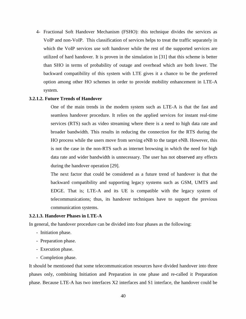
40

4- Fractional Soft Handover Mechanism (FSHO): this technique divides the services as

VoIP and non-VoIP. This classification of services helps to treat the traffic separately in

which the VoIP services use soft handover while the rest of the supported services are

utilized of hard handover. It is proven in the simulation in [31] that this scheme is better

than SHO in terms of probability of outage and overhead which are both lower. The

backward compatibility of this system with LTE gives it a chance to be the preferred

option among other HO schemes in order to provide mobility enhancement in LTE-A

system.

3.2.1.2. Future Trends of Handover

One of the main trends in the modern system such as LTE-A is that the fast and

seamless handover procedure. It relies on the applied services for instant real-time

services (RTS) such as video streaming where there is a need to high data rate and

broader bandwidth. This results in reducing the connection for the RTS during the

HO process while the users move from serving eNB to the target eNB. However, this

is not the case in the non-RTS such as internet browsing in which the need for high

data rate and wider bandwidth is unnecessary. The user has not observed any effects

during the handover operation [29].

The next factor that could be considered as a future trend of handover is that the

backward compatibility and supporting legacy systems such as GSM, UMTS and

EDGE. That is; LTE-A and its UE is compatible with the legacy system of

telecommunications; thus, its handover techniques have to support the previous

communication systems.

3.2.1.3. Handover Phases in LTE-A

In general, the handover procedure can be divided into four phases as the following:

- Initiation phase.

- Preparation phase.

- Execution phase.

- Completion phase.

It should be mentioned that some telecommunication resources have divided handover into three

phases only, combining Initiation and Preparation in one phase and re-called it Preparation

phase. Because LTE-A has two interfaces X2 interfaces and S1 interface, the handover could be

41

classified based on these interfaces. While X2-based handover obviously happens between eNBs

only when there is no need to change the serving MME as a consequence for handover operation,

S1-based handover takes place when the MME is changed because of the handover. It further

affects the network since it reaches MME node, and it takes more time than the X2-based HO.

The main different between those two sorts is the network signaling that happened between

source and target eNBs and in some cases core network (CN). However, the signaling over the

radio link has no change in which same RRC procedure are conducted, and the UE behavior is

unchanged [33]

1- Initiation phase: in this phase, the source eNB chooses from the neighboring competitive

eNBs as a target where the UE will switch to. In addition, the serving eNB decides when the

UE has to be moved to the chosen target eNB [33].Figure.3.6 explains the initiation phase.

Figure 3.6 X2 Initiation Phase [34]

2- Preparation phase: this is the phase where not only the measurement reports are important

as input to the handover decision to be taken, but also the MME could provide another

important input to the handover decision. This input is a handover specific list of competitive

target eNBs used by the serving eNB to filter the target eNBs [33].The handover decision is

important to specify whether the handover is X2 type or S1 handover. X2-based handover in

this phase has the following procedure as shown in Figure.3.7.

42

Figure 3.7 X2 based Handover –Preparation Phases [33]

Source eNB is responsible for initiating the handover request through X2 interface, so it sends a

request to the target eNB asking for the permission to hand its user and prepare the HO

operation. Generally, in the handover preparation phase, the serving eNB informs the target eNB

about all the inter-node RRC-information related to the served UE. This information involves

settings of RRC that are already being applied, RRM specific information of the UE, and the

information about the connected UE’s capability of radio access. These details are required to

configure the target eNB to be capable of serving the UE during the handover and after

completing the HO operation. To recover the probability of handover failure, the source eNB

includes other important information via inter-node RRC information called re-establishment

information used in reestablishing the connection. Via X2 interface, target eNB acknowledges

the handover request of the source eNB directly using Handover Request Acknowledgment

message.

43

In S1-based handover, on the other hand, the source eNB sends the initiated message

(Handover Request Message) to the MME through S1 interface informing about the need

to trigger the handover preparation with the target cell. Handover Request Message has

valuable information such as priority and QoS that it is important to configure the target

eNB to be ready to serve the transferring UE.

Figure 3.8 S1 based Handover – Preparation Phases [33]

44

While the target eNB gets the Handover Request Message, it can accept or refuse the request of

handover depending on the feedback in the Handover Request Message. In another words, target

eNB performs the admission control relying on the available radio resources, eNB configuration

and information in Handover Request Message. If there is a one affordable enhanced radio

access bearer (E-RAB) at the target eNB, this eNB prepares the required resources to serve the

new transferred UE and acknowledges the source eNB by sending HO Request ACK message.

ACK message is sent to the MME. It contains the required configuration changes that have to be

aware by the UE while moving to the target eNB. Finally, MME sends back an explicit message

called “Handover Command message” to the source eNB containing the RRC connection

configuration through S1 interface. S1 based handover is shown in Figure.3.8.

3- Execution Phase

It is a phase in which the target eNB commands the source eNB to start the handover by sending

the RCC reconfiguration message. The source eNB forwards without updating the

reconfiguration message received from the target eNB to the UE. The content of the

reconfiguration message is the mobility control info (Handover Command) which is used to

order the mobile to reset the current MAC and RRC sessions and to signal with new eNB. The

Handover Command includes information such as used frequency, target cell downlink and

uplink bandwidths, and the target eNB physical ID. It also has new C-RNTI that is utilized at a

target eNB to define the UE and provide the required information to access the common

channels (RACH). Moreover; the security information is included in the mobility control info

message. If there is data being under transmitting while the handover occurs, the source eNB

forwards the data to the target eNB to prevent data loss. In the X1 based handover, the data is

sent through the GTP tunnel directly from the source to target eNBs. Unlike X1 based handover,

the S1 handover avoids data loss during the handover operation by sending the data via indirect

route through S-GW.

It should be notice that there is a time limit for handover operation that is set using a timer. When

the timer is expired while the handover is still occurring, the UE announces that the handover is

unsuccessful and starts the procedure of reconnection establishment to cope that failure. Any

delay in handover can be reduced by preventing UE from reading the target cell system

information before accomplishing random access operation. After the handover is completed, all

45

required system information could be requested by the transferred UE from the target eNB. The

handover exaction is shown in Figure.3.9.

Figure 3.9 Handover Execution Phase [33]

4- Completion Phase

It is the phase that from the UE perspective is finished when it sends the RRC connection

reconfiguration complete message. In comparison, from the system point of view is that when

the network performs further procedures such as releasing the radio resource of the source eNB

and transferring the data to the target eNB. However, different procedures are taken place in this

phase regarding whether X1 based handover or S1 based handover. In X1 based handover, the

completion indication message called Path Switch Request message is sent by the target eNB to

MME. Similarly, in S1 based handover, but the message is called Handover Notify message.

Upon MME getting either message, it connects with the serving gateway (S-GW) to arrange data

switching from the serving eNB to the target cell.

46

The source eNB releases UE and the used radio resources when it is notified by the target eNB in

X1 based handover or MME in S1 based handover that the handover is completed. This can be

conducted using the UE Context Release message or UE Context Release Command message

respectively. As aforementioned before, all handover phases are limited by handover timers.

These timers are used to guarantee that the handover operation is conducted properly. For

instance, if the source eNB does not receive a completion messages from other participating

nodes (target eNB or MME as explained before), the source eNB will force the MME to send the

UE Context Release Command by sending the Context Release Request message. Figures 3.10

and 3.11 show the completion phase in X1 based handover and S1 based handover respectively.

Figure 3.10 Handover Completion Phase-X1 based Handover [33]

47

3.2.2. Admission Control

To satisfy SLA and QoS that agreed with the networks’ customers in the modern

telecommunication networks, admission control (AC) is applied which is one of the fundamental

and crucial method. AC is not 3GPP standard in which different providers use various AC

algorithms to meet their network and customer needs. Therefore, it is specified by the vendor for

each eNB in the system to guarantee that the newly admitted traffic will not affect the current

applied QoS for the served flows [23]. Different restrictions limit AC decision, for example, the

required QoS for both new and admitted bearers, the affordable radio resources, and the type of

traffic. Mainly, AC operation accepts or rejects the requested EPS - Evolved Packet System

bearers in the system. EPS contains a profile that clarifies the QoS requirements involving

several numbers of auto-modified parameters.

Figure 3.11 Handover Completion Phase-S1 based Handover [33]

48

The following details clarify EPS auto-modified downlink parameters:

1- QoS Class Identifier (QCI). It is one of the most important parameters that have different

values for other parameters such as packet error rate of layer 2, packet latency of layer 2 and

priority of scheduling. These parameters can achieve the required HOL delay target by

prioritizing different queues. Resources allocation is based on QCI, for example, if UE uses

VoIP and browsing services, the higher priority (VoIP) is allocated resources firstly then the

browsing. 3GPP has defined nine QCIs with their characteristics as shown in Table 3.1

QCI# Bite Rate Type Priority L2- Packet Error Rate L2-Packet Delay Example services

1 (GBR) 2 10-2 100ms Conventional voice

2 (GBR) 4 10-3 150ms Conventional video

3 (GBR) 5 10-6 300ms Buffered streaming

4 (GBR) 3 10-3 50ms Real-time gaming

5 (non-GBR) 1 10-6 100ms IMS signaling

6 (non-GBR) 7 10-3 100ms Live streaming

7 (non-GBR) 6 10-6 300ms Buffered streaming, email,

8 (non-GBR) 8 10-6 300ms browsing, file download,

9 (non-GBR) 9 10-6 300ms file sharing, etc.

Table 3.1 QCI Parameters for EPS Bearer QoS Profile [3]

2- Guaranteed Bit Rate (GBR). It is the parameter that grants a certain bit rate to the bearer that

is identified as GBR bearer. In the case of non-guaranteed bit rate bearer sort, another

parameter called AMBR (Aggregate Maximum Bit Rate) is assigned. A bearer can be

allocated a maximum bit rate (MBR) in certain conditions.

3- Allocation Retention Priority (ARP). It is sixteen integer values starts 1 and ends with 16.

APR performs admission control decisions prioritization. There is confusion about the

different between ARP and QCI. APR relates to services and bearers allocation while as

mentioned before, QCI concerns about resource allocation. An example of ARP is that UE

aims to setup VoIP (higher ARP priority) along with browsing service; the eNB will reject

the browsing request and admit only the VoIP request in order not to be overloaded.

49

The Radio Resource Management at eNB is responsible for managing and handling different

load conditions (i.e., low load, moderate load and excessive load). At the excessive load

condition, occurrence of a received packet blocking is highly possible. On the other hand, in the

situation of low load there is no possibility for packet blocking since the active UEs are few, in

turn, the amount of transmitted data is small and the inter-cell interference level is at its

minimum value. Moreover, the minimum QoS requirements for the active users are guaranteed.

In LTE network, the system starts utilizing all available physical radio resources as the number

of admitted UEs into the system increases. Additionally, in order to satisfy QoS constraints for

various users, the operation of layer 2 scheduling for more UEs is increased. At a full load using

all available PRBs, there is a possibility that the system may admit more UEs while marinating

agreed QoS level of the current served users unchanged. The packet scheduler entity will allocate

fewer resources to the best effort bearers if the allocated resources for the users with stricter QoS

(i.e., GBR) increase. However, further optimizations may be required as the system is loaded

with more users. Due to the fact that there are both RT traffic and Non-RT traffic in one

scenario, the switching between L2 scheduling (dynamic scheduling) and L3 scheduling (semi-

persistent scheduling) is beneficial. It is obvious that more regulation is required while the traffic

increases. However, the admission control entity will begin blocking arriving new users’ traffic

although the RRM functionalities (i.e., scheduling) aim to increase cell capability to serve more

users with their associated traffic types [24].

3.2.3. Packet Scheduling (PS)

Radio Resource Management entity at the eNB for a multi-carrier advanced LTE network is

shown in Figure.3.12. Essentially, the main two parts of RRM are: carrier component (CC)

allocation and Packet Scheduling (PS). Carrier component allocation is that RRM selects and

allocates CCs for each UEs while Packet Scheduling (PS) is responsible for assigning radio

resources to each user within each CC. The PS decision is made at each transmission time

interval TTI (1 ms) or at resource-block-pair (RB of o.5 ms subframe over 180 kHz), taking into

account the feedback from the users using Channel Quality Indicator CQI. It helps eNB to

estimates the reachable throughput for each user using the feedback information. Furthermore,

eNB informs the users about the affordable allocated resources [25]. Even though the load status

and the user past throughput are present in the eNB, only uplink CQI feedback is useful from the

eNB point of view to make a decision about resources allocation.

50

One the other hand, each UE measures the received signal to interference ratio (SINR) carried on

the reference signal sent by the serving base station in the downlink direction. A user is usually

moving in the cell coverage; thereby the time-selective fading and multi-path fading natures

exist. This results in different calculated SINR values on each subcarrier at each Transmission

Time Interval. The measurements, specifically effective SINR values, aid UE to feedback its

channel status to the serving eNodeB. The values of effective SINR are used by the base station

to select modulation and coding scheme (MCS) in the downlink packet direction [35].The later

(MCS) is related to the data rate determination, in which the bits that are supported by users are

determined based on MCS. Not only finding out the data rate in two contiguous RBs as

mentioned before, but also selecting the priority of the users in channel-depending scheduling is

supported using the effective SINR. The packets for each user are buffered upon arriving at

eNodeB, and time stamped by the scheduler. Then, the First-In-First-Out (FIFO) technique is

used to handle user’s packets. To control the queuing operation and avoid long waiting time for

the packet, Head Of Line (HOL) packet latency has been utilized. It is the different between the

current time of a certain packet and arrival time of the same packet [35]. The HOL delays are

assigned for different traffic types based of the classification of the traffics as Real Time (RT)

and Non-Real Time (NRT) services. The threshold point of the HOL is when it exceeds the

delay’s deadline; at this point the queued packets are deleted.

Figure 3.12 RRM Framework in LTE-A [25]

51

Packet scheduling can be classified into two types: in the downlink direction which is the most

important one since it is related to eNB and performed by RRM, and in the uplink direction

which is conducted by UE.

3.2.3.1. Downlink Packet Scheduling

Due to the fact that there is a limited number of available radio resources for each network

operators, PS is proposed to meet the goal of maximizing the utilization of these resources, and

in the meantime satisfying the agreed level of QoS for connected UEs. The decision of

scheduling is made at each transmission time interval; hence, UEs are allocated different amount

of radio resources blocks (PRBs) each TTI according to their requested services. The decision

not only includes PRBs allocation, but also Modulation and Coding Schemes (MCS) or what so-

called link adaptation to be used in the downlink packets communication. PDCCH is used to

carry the allocated resources to the users. The link between the eNB and users has two main L2

flows: one carries the data (data plane), and one carries the control information (control plane).

In the downlink direction, there is interaction between the packet scheduler and Hybrid ARQ

entity as shown in Figure.3.13. Retransmission is managed by Hybrid ARQ manager and

scheduled dynamically by the PS in frequency/time domains. While the frequency domain

scheduling means that the user is allocated PRBs, the time domain scheduling means that the

user is selected to be scheduled at TTI. The scheduler serves all UEs and ensures there is fairness

among them by sending either a new flow or awaiting Hybrid ARQ flow to each scheduled UE

in one TTI. If the scheduler schedules both flows simultaneously to one user, other users in the

system will suffer starvation [24]. Figure 3.3 also shows Link Adaptation mechanism which

interacts with scheduling operation to provide the suitable modulation and coding schemes

(QPSK, 16QAM or 64 QAM) according to the utilized physical resource blocks for each UE.

The CQI receiving from the users and QoS at the eNB are used in LA decisions [3].

52

Figure 3.13 Interactions between HARQ, PS and LA [3]

The higher channel quality user is the selected user to be scheduled in the frequency domain

scheduling schemes (FDPS) since frequency selective fading is achieved. Accordingly, any

PRBs with deep fade are avoided by FDPS [24] as shown in Figure.3.14.

Figure 3.14 Frequency DPS Concept [3]

There are two methods that have been used to conduct the packet scheduling: per each carrier

component (CC) so-called independent scheduling or cross CC scheduling. The cross CC

scheduling is more complex than independent scheduling since it based on all other available

CCs in the system. This is; the metric of scheduling is calculated differently in each one [25].

53

Independent CC PS. the similarity to the traditional PS in a single carrier system is shown

in this method, in which there is no need to consider the transmission characteristics on

other CCs. Dividing the instantaneous throughput by the average throughput of the

selected user is the used method to calculate the scheduling metric.

(3.1)

the estimated throughput for user k on ith

CC at the jth

PRB group is represented by ,

the average throughput at the past for the same user on the same CC is represented by

.

The equation is considered to Rel8. For LTE-A, since it could be assigned more than one

CC, the same equation is used multiplied by total number (N) of allocated CCs for LTE-

A UEs.

Cross-CC PS. considering the transmission characteristics of all CCs, PS fulfills better

resource allocation than independent packet scheduling. Unlike independent PS, the past

user throughput over the all aggregated CCs is taken into account to calculate the

scheduling metric.

(3.2)

3.2.3.2. Packet Scheduling Algorithms in Downlink Direction

The packet scheduling algorithms are various based on RT and NRT services. The common

adopted PS algorithms according to [26] and [35] are:

First-In-First-Out (FIFO). The user with the highest packet delay HOL at each TTI is

given transmission priority. It provides considerable fairness among users who have

similar packet’s characteristics such packet size and channel status [35].

Round Robin (RR). In this algorithm, transmission time interval is divided equally

among users, in which each user is allocated equal time to transmit its packet in a circular

order. This algorithm is similar to FIFO that provides a high level of fairness. However,

the throughput performance in RR is higher than FIFO.

54

Maximum Rate scheduler (Max Rate).Once the highest achievable data rate is reached,

the UE is selected to be scheduled. Equation 3.3 expresses Max Rate scheduling

algorithm:

(3.3)

is the reachable data rate for a UE denoted by k at time t based on the received

SINR at eNB where and SINR are directly proportional. Because this algorithm is

designed to schedule users with maximum data rate regarding with their best channel

conditions, it provides the best system throughput. Accordingly, the poor fairness is

obvious in Maximal Rate PS algorithm since the lower received SINR value the less

opportunity for user to be selected for transmission. Moreover, UE’s resources starvation

could happen since the user is probably never selected for scheduling.

Proportional Fair (PF). PF algorithm balances the system performance between the

throughput and the fairness among users, giving a trade-off between them. A user is

allocated resources if it has the maximum ratio between the instantaneous achievable rate

and the transmission rate divided by the average throughput.

(3.4)

, is the average throughput of user k at time slot t. It is calculated by considering the

window size as follows:

(3. 5)

when UE k is selected for transmission, the value equals 1, otherwise the value

equal 0.

The reason behind a good throughput and fairness performance is that PF algorithm

performs incorporation for the feasible data rate with an average throughput [35].

Frame Level Scheduler (FLS). The FLS is a combined algorithm that has two levels of

scheduling; upper and lower level, thereby, separate algorithm for each one. Upper level

is less complexity in allocation of resources since it depends on the theory of discrete

time linear control. The task of the upper level is that satisfying delay constraint by

calculating the amount of data that each real-time source should send within a single

55

frame. Equation 3.16 shows the calculation of the aforementioned amount of data at

upper level of FLS. The lower level, on the other hand, is more complexity since it uses

PF algorithm to allocate resources to the UE [36].

(3.6)

denotes the data amount that is sent within the frame n for flow. is the

filtered signal by which is a time-invariant linear filter with pulse response.

According to the results in [11] cited in [36], the FLS provides restricted delays and

lower PLR values for a video traffic ,thereby, the performance of FLS ensures the best

quality of the video service for the scheduled users.

Modified-Largest Weighted Delay First (MLWDF). This algorithm is introduced to

support Real Time services. The metric of scheduling is shown :

(3.7)

where;

(3.8)

HOL packet delay of user at time is denoted by , is the delay’s deadline that

the maximum HOL probability to exceed it is .

The benefit of MLWDF is that using PF properties along with the HOL packet delay

consideration introducing a better throughput, fairness and Packet Loss ratio than PF

algorithm.

Exponential/Proportional Fair (EXP/PF). The aim of proposing this algorithm is to be

used for multimedia services for both Real Time and Non-Real Time services

simultaneously. The metric for RT and NRT is shown below:

(3.9)

where,

(3.10)

(3.11)

56

denotes the average number of packets queued in the buffer at time t, k and in equation

(3.11) are predefined values, is the highest HOL packet delays for the packet awaiting for

RT services, and is the maximum delay of RT service users.

Although EXP/PF is adopted for both real time and non-real time users, it precedes RT users

over the NRT if the RT users’ packets reach the transmission threshold[35].

Logarithmic (LOG) Rule scheduler. The LOG Rule allocates the resources to the

scheduled UEs increasing current throughput by supposing the channel status and traffic

arrival are realised. The main propose that LOG Rule is designed to provide QoS

balancing in term of robustness and mean delay. According to [13] cited in [36], the

simulation results prove that LOG Rule is a superior algorithm that has the best packet

delay decreasing. Although this algorithm is an experimented practically as a good

solution, it is not proven as an optimal method for mean-delay achievement [36]. LOG

Rule and EXP Rule algorithms are a type of opportunistic scheduling, in which they

exploit the desirable channel to schedule the active users, for example, the users with the

highest rate.

Exponential (EXP) Rule. Similarly to LOG Rule, the goal of proposing this algorithm

was basically to satisfy QoS requirements in the wireless network. The balance between

the throughput and mean-delay is conducted by maintaining minimum value of delay and

at the mean time a considerable value of throughput, thereby, mean-delay is obtained. It

works on the concept of wireless channel sharing among arrival users and queues their

data as a random stream to be prepared for transmission. This scheduler enables users

accessing the services during each time interval. Optimal throughput is determined

according to [12] cited in [36]. The difference with LOG rule is that there is no previous

estimation of traffic arrival and channel statistics. However, the EXP Rule explicitly

utilizes received channel statistics information and guarantees achieving stable queues.

Two exponential rules have been introduced in this scheme: EXP Waiting time (EXP-W)

and EXP Queuing (EXP-Q). The algorithm selects one rule at a time for scheduling users

with different fix positive parameters (i.e., and ) as

shown in equations (3.12) and (3.13).

57

(3.12)

(3.13)

where,

and

(3.14)

is the total number of queued users who are selected for transmission at time .

3.2.3.3. Uplink Packet Scheduling

In the UL scheduling, the user is aware of packets scheduling, and it has to buffer the arrived

flows. The finite size of the users’ buffers degrades the performance of scheduling operation at

the UEs since the base station in LTE is unaware of the size of UEs’ buffer. Not only the

buffering limitation at the UEs, but also the power limitation in uplink direction emerges another

constraint for the uplink scheduling. Obviously, eNB power in the downlink is much higher than

the UEs power. On the other hand, resource allocation restriction exists since single carrier

modulation has been used with uplink scheduling. In consequence, solely adjacent PRBs can be

assigned to each UE.

CSI report is the feedback information that is used to choose the modulation and coding scheme.

Relying on the Sounding Reference Signal (SRS) sent by the UE, the CSI is determined. The

integration in the uplink direction between RRM, LA and PS is shown in the Figure.3.15. Link

Adaptation compromises adaptive modulation and coding, Outer Loop Link Adaptation (OLLA)

and Power Control (PC). PS has scheduling request, buffer status report and Adaptive

Transmission Bandwidth (ATB). There is also a relation as seen in Figure.3.15 between LA and

PS, in which PC and AMC of LA interact with PS. That is, on the channel state, the packet

scheduler receives required information related to the transmission bandwidth from AMC for a

certain user. Uplink PC main purpose is that maintaining SINR to a certain level called SINR

threshold according to the agreed QoS while limiting the ISI [3].

58

Figure 3.15 Uplink RRM Functionalities inter-work with LA and PS [3]

3.2.4. Power Control (PC)

The Orthogonal Frequency Division Multiple Access OFDMA and the Single Carrier Frequency

Domain Multiple Access are the radio technologies used in LTE and LTE-A. The reason behind

adopting OFDMA and SC-FDMA in the modern networks is that to elevate the effect of intra-

cell interference that is the interference between users within a single cell. The orthogonality is

used to avoid users having the same peak at a certain point of time instead only one user could be

served at that peak. However, another interference causing by adjacent cells, which is well-

known as inter-cell interference cannot be negligible, introducing a real challenge since

orthogonal modulations is not designed to solve such interference. It requires other mechanisms

to solve it that the power control is one of them. Since the PC limits the cell boundary, it can

eliminate the impact of inter-cell interference. The control of the transmitted power can be

performed at UE in the uplink direction or the base station (eNodeB) in the downlink direction

[32].

59

The UE transmits the power in the uplink direction based on the equation (3.15).

(3.15)

Where and are the UE’s maximum allowed transmit power based on the UE power

classification and the number of allocated physical radio resources on the PUSCH respectively.

UE measures the downlink path loss which is denoted by , denotes closed-loop power

control correction that eNB transmits (details can be found in 3.8.4 of [37] ).

are parameters of PC. The can be computed as follows [32]:

(3.16)

where is the target of open loop SNR (details can be found in 3.8.3 of [37]), and are

the PRB noise power and the number of PRBs required to fulfill the target SNR with full power,

respectively.

UE initiates a transmission power based on and the calculation of the path loss

performed by the UE. Since eNB signals the value of to UE who already has completed

setting the initial power, it does not contribute in the initiation operation. Hence, by ignoring the

value of as well as , the equation (3.15) can be written as following:

[dBm] (3.17)

It represents the calculation of the initial transmitted UE power.

The number of scheduled PRBs is denoted by in which the UE allocates power based on

PRB. That is; the amount of power for each PRB is equal.

To calculate the UE’s Power Spectral Density (PSD) to each PRB, the value of is

neglected and the equation (3.17) is changed to be as the following [32]:

[dBm/PRB] (3.18)

The power control has two types depends on the value of in Equation (3.18). If the value of

is between 0 and 1, the power control mode is called fractional power control.

When the value of is 1, the power control mode is called conventional power-control. Other

types of power control have to be mentioned here which they are: open loop power control and

close loop power control. Detailed descriptions of the power control modes can be found in [37].

60

3.2.5. Balancing of Carrier Load

LTE and LTE-A can coexist together in the same network due to the backward compatibility of

LTE-A. As mentioned before the maximum prescribed bandwidth of LTE is 20MHz. To achieve

LTE-A bandwidth that is 100 MHz, 5 CCs of Rel8 have to be aggregated. In LTE, UEs are

allocated a single CC while in LTE-A UEs are assigned multiple CCs based on their channel

conditions. The flowchart in Figure.3.16 explains the LTE-A’s eNB classification operation

whether the case of LTE UE or LTE-A UE to make a decision of radio resources allocation on

CC(s). To balance the load on all available CCs, UEs are equally scheduled on all CCs using a

smart load balancing mechanism. This could guarantee an exploitation of all affordable resources

on CCs. The following sections discuss the load balancing methods.

Figure 3.16 eNB Classification for LTE Rel 8 and LTE-A Arrival UEs [25]

3.2.5.1. Carrier Load Balancing

As aforementioned, Rel 10 has a backward compatibility with Rel8. For a user in LTE, the

system allocates one CC while the system could allocate number of CCs based on the QoS and

user’s feedback reports for a user in LTE-A. The CCs’ balanced distribution among the served

users can be performed by deploying balancing methods as the following [27]:

61

Round Robin (RR) Balancing Method: in this method, the user is allocated 1 CC. The

newly arrived user is assigned the least exploited carrier by other users. The aim of that is

to divide UEs equally on all available CCs. An issue of this method is that the CCs load

could have a minor difference due to the probability of uneven number of users or due to

the fact that the users could free up the allocated CC at random.

Mobile Hashing (MH) Balancing Method: also well-know independent carrier channel

assignment. Similarly to RR, a user is allocated 1 CC. However, MH differentiates from

RR by using hash algorithm calculations of the terminals. The purpose of considering the

output of hash values is that providing a long-term CCs load balancing. In order to

achieve that, it requires uniformly distributing of the values of hash outputs among a

limited set that CC indices are mapped directly on it.

3.2.6. Interference Management

The interference is one of the big challenges encounter LTE and LTE-A especially with HetNets,

in which the small cells (Pico, Femto, RRH or relay node) use the same carrier frequency of the

Macro cells. The higher power eNB (Macro cell) is overlaid with small lower power cells that

are used with less care or uncoordinated manner. The technology that has been implemented to

relieve the impact of the interference between adjacent cells is the Inter-cell Interference

Coordination (ICIC). ICIC is the operation in which the interference could be mitigated if high

transmission power on PRBs is avoided. That is; the users on the cell edge can be served in the

neighboring cells. There are two classes of ICIC schemes based on the way it deals with the

interference. The first class is reactive ICIC that is responsible for monitoring the system. That

is; if it observes a high level of the interference, the suitable procedures will be implemented.

Examples of the reactive ICIC are packet scheduling and power control for the purpose of

interference reduction to an appropriate status. The other class is proactive that is responsible for

avoiding the interference before the high level is detected. That could be performed through the

eNBs coordination in which neighboring eNBs receives feedback from the eNB informing about

the future plans of scheduling its users. These reports can be considered to avoid low value of

Signal- to- Interference Ratio (SIR) that could occur [3]. There is a relation between proactive

ICIC and Relative Narrowband Transmit Power (RNTP). RNTP is a PRB’s peak downlink

transmission power. Neighboring eNB receives RNTP through X2 interface, then these RNTP

62

values can be utilized by the neighboring eNB to make a decision for scheduling its UEs.

Especially, the UEs who are more likely existed at the cell edge have a high probably to suffer

from neighboring cells interference (LTE case) or small cells and neighboring cells (LTE-A

case).Thus, RNTP facilitates the proactive ICIC in the downlink direction. Various parameters

are considered to perform the proactive and reactive ICIC in the uplink direction. The High

Interference Indicator (HII) and Overload Indicator (OI) are used to support proactive and

reactive ICIC schemes respectively. HII carries a serving eNB message to its adjacent cells over

X2 interface indicating which PRBs will be exploited for scheduling boundary cell UEs such as

the higher interference expectation of PRBs from the neighboring cells perspective. Hence, the

adjacent cells allocate those PRBs to the lower interference UEs. This is the reason that why HII

is seen as a technique of proactive ICIC.

As mentioned before, OI is related to reactive ICIC scheme and its task essentially is to carry

reports of the measured uplink interference on reporting eNB’s PRBs at three levels (low,

average and high). The adjacent eNBs deal with these measurements once they are received by

adjusting the scheduling behavior to the extent that enhances the SIR of the OI releasing eNB

[11].

3.3. Summary

RRM is the entity that is mainly responsible for the following: Handover, Admission Control,

Packet Scheduling, Power Control and Interference Management. Thus, it plays a vital role in the

most recent LTE and LTE-A networks where the most important functions in managing a mobile

network is performed at eNB using RRM. While the LTE-A is introduced through HetNets, the

importance of RRM has increased due to the increment of the issues related to interference,

handover and scheduling. Since the simulation and practical outcomes in the next chapter mainly

concern with Handover and Packet Scheduling and its algorithms, the focus in this chapter is on

these RRM functionalities.

63

References

[1] H. Holma and A. Toskala, Wcdma for Umts vol. 4: Citeseer, 2000.

[2] A. Ghosh and R. Ratasuk, Essentials of lte and lte-a: Cambridge University Press, 2011.

[3] H. Holma and A. Toskala, LTE for UMTS: OFDMA and SC-FDMA based radio access:

John Wiley & Sons Inc, 2009.

[4] K. Sandrasegaran. (2012, 5 Aug 2012). 4G and Long Term Evolution (LTE). Available: <

www.online.uts.edu.au/49048/LTE >

[5] H. G. Myung, "Introduction to single carrier FDMA," 2007.

[6] J. Hågstrand, P. Karlsson, and O. Silverplats, "Proof of concept implementation of

UMTS long term evolution," 2007.

[7] M. Rumney, "3GPP LTE: Introducing Single-Carrier FDMA," Agilent Technologies

White Paper, 2008.

[8] H. Holma and A. Toskala, LTE Advanced: 3GPP Solution for IMT-Advanced: Wiley,

2012.

[9] A. Lucent. (2009, 20 Aug 2012). The LTE Network Architecture A comprehensive

tutorial. Available: www.alcatel-lucent.com

[10] S. Sesia, I. Toufik, and M. Baker, "LTE–The UMTS Long Term Evolution," From

Theory to Practice, published in, vol. 66, 2009.

[11] E. Dahlman, S. Parkvall, and J. Sköld, 4G LTE/LTE-Advanced for mobile broadband:

Academic Press, 2011.

[12] J. Löfgren. (2009, 3 Sep 2012). LTE Radio Interface ArchitectureAvailable: <

http://www.eit.lth.se/fileadmin/eit/courses/phd003/Slides/Ch15.pdf >

[13] H. G. Myung, "Technical overview of 3GPP LTE," Polytechnic University of New York,

2008.

[14] M. Sauter, FROM GSM TO LTE AN INTRODUCTION TO MOBILE NETWORK AND

MOBILE BROADBAND. United Kingdom: John Wiley & Sons Ltd, 2011.

[15] C. Cox, AN INTRODUCTION TO LTE, LTE-ADVANCED, SAE AND 4G MOBILE

COMMUNICATION. United Kingdom: John Wiley & Sons Ltd, 2012.

[16] E. Dahlman, 3G evolution: HSPA and LTE for mobile broadband: Academic Press, 2008.

[17] D. Kimura and H. Seki, "Inter-Cell Interference Coordination (ICIC) Technology,"

FUJITSU Sci. Tech. J, vol. 48, pp. 89-94, 2012.

[18] B. Y. B. Cho. (2011, 23 Aug 2012). LTE DL Transmission. Available: <

http://www.scribd.com/doc/86351165/2-LTE-DL-Transmission >

[19] 3GPP. (2011, 5 Sep 2012). Technical specification Group Services and System Aspects;

Multimedia Broadcast/Multicast Service (MBMS); Architecture and functional

description version 9.6.0 (Release 9). Available: < http://www.3gpp.org/ftp/Specs/html-

info/23246.htm >

[20] 3GPP. (2011, 15 Aug 2012). Technical Specification Group Radio Access Network;

Feasibility study for Further Advancements for E-UTRA (LTE-Advanced) version 10.0.0

(Release 10). Available: < http://www.3gpp.org/ftp/specs/html-info/36912.htm >

[21] I. F. Akyildiz, D. M. Gutierrez-Estevez, and E. C. Reyes, "The evolution to 4G cellular

systems: LTE-Advanced," Physical Communication, vol. 3, pp. 217-244, 2010.

64

[22] 3GPP. (2010, 10 Sep 2012). Technical Specification Group Radio Access Network;

Evolved Universal Terrestrial Radio Access (E-UTRA); Further advancements for E-

UTRA Physical layer aspects version 9.0.0 (release 9). Available: <

http://www.3gpp.org/ftp/Specs/html-info/36814.htm >

[23] E. Z. Tragos, G. Tsiropoulos, G. T. Karetsos, and S. A. Kyriazakos, "Admission control

for QoS support in heterogeneous 4G wireless networks," Network, IEEE, vol. 22, pp. 30-

37, 2008.

[24] K. I. Pedersen, T. E. Kolding, F. Frederiksen, I. Z. Kovács, D. Laselva, and P. E.

Mogensen, "An overview of downlink radio resource management for UTRAN long-term

evolution," Communications Magazine, IEEE, vol. 47, pp. 86-93, 2009.

[25] Y. Wang, K. I. Pedersen, T. B. Sørensen, and P. E. Mogensen, "Carrier load balancing

and packet scheduling for multi-carrier systems," Wireless Communications, IEEE

Transactions on, vol. 9, pp. 1780-1789, 2010.

[26] A. Hecker, M. Garcia-Lozano, and J. F. Monserrat, "Resource Management in 4G

Networks," Pervasive Mobile and Ambient Wireless Communications: COST Action

2100, p. 461, 2012.

[27] Y. Wang, K. I. Pedersen, P. E. Mogensen, and T. Sorensen, "Carrier load balancing

methods with bursty traffic for LTE-Advanced systems," 2009, pp. 22-26.

[28] Y. Lee, J. Zhao, and H. Qu, "A combined handover scheme for LTE-advanced system,"

2012, pp. 154-157.

[29] I. Shayea, M. Ismail, and R. Nordin, "Advanced handover techniques in LTE-Advanced

system," 2012, pp. 74-79.

[30] H. Lee, H. Son, and S. Lee, "OFDM-Based Semi-Soft Handover for High Data Rate

Services," in Personal, Indoor and Mobile Radio Communications, 2007. PIMRC 2007.

IEEE 18th International Symposium on, 2007, pp. 1-5.

[31] J. Chang, Y. Li, S. Feng, H. Wang, C. Sun, and P. Zhang, "A fractional soft handover

scheme for 3GPP LTE-advanced system," in Communications Workshops, 2009. ICC

Workshops 2009. IEEE International Conference on, 2009, pp. 1-5.

[32] B. Muhammad, "Closed loop power control for LTE uplink," Blekinge Institute of

Technology School of Engineering, 2008.

[33] June Yi, S.C., YoungDae Lee, SungJun Park, SungHoon Jung, “Radio Protocols for LTE

and LTE-Advanced”, 2012.

[34] Penttinen, Jyrki , “LTE/SAE Deployment Handbook”, 2011.

[35] Nguyen, Sinh Chuong , “Packet Scheduling for LTE-Advanced”, Master thesis 2011.

[36] Shaoo, Biswapratapsingh, “Performance comparison of packet scheduling algorithms for

video traffic in LTE cellular network”, PInternational Journal of Mobile Network

Communications & Telematics ( IJMNCT) Vol. 3, No.3, June 2013.

[37] AL-Jaradat, Huthaifa, ‘Radio Resource Management in LTE and LTE-A’, Master thesis

2013.

65

4. Chapter 4: LTE-Sim Heterogeneous Network Deployment

4.1. Introduction

In the Long Term Evolution so-called LTE, the requirements for larger coverage area, more

capacity, and high data rate and low latency have led to search for cost-effective solutions to

meet these demands. Hence, the development in the telecommunication networks has adopted

different directions to enhance the LTE system taking into account the International Mobile

Telecommunications (IMT-2000) standards that have to be satisfied [1]. Network-based

technologies such as Multiple Input and Multiple Output MIMO/ advanced MIMO and

Transmission/Reception Coordinated Multi-Point CoMP are LTE enhancements that introduce

LTE Advance (LTE-A). Other fewer cost enhancements based on air interfaces are proposed,

such as improving spectral efficiency involving using Heterogeneous networks (HetNets).

HetNets are small and lower power cells within the main Macro cells with different access

technologies to close up the network to the end users and increase their expectation

[16].According to [2], there are two main practical HetNets classes: Macro with Femto and

Macro with Pico. Femto and Pico are the small and lower power cells. To save the cost,

operators use the same carrier frequency in the large and small cells which, on the other hand,

proposes interference challenges. Figure.4.1 gives the main concept of HetNets. To clarify, user

in LTE is well-known as a UE.

Figure 4.1 an Example of HetNets

66

In LTE and LTE-A, the element that is responsible for Radio Resources Management (RRM) is

enhanced Node Base station (so-called eNB). The eNB does all required management including

Packet Scheduling (PS) which is the focus in the paper. PS can guarantee the agreed quality of

service demands (QoS) because it is responsible for the best and effective utilizing of the

affordable radio resources and in charge of data packets transmission of the users[3].

3rd Generation Partnership Project (3GPP) has left the scheduling algorithms to be a vendor

specific according to user’s requirements and network capability. Therefore, various PS

algorithms have been proposed depending on the traffic sorts and provided services. PF,

MLWDF and EXP/PF algorithms [4][5][6] are used in this paper to study and compare between

the system behaviours in HetNets (single Macro with 2 Pico cells) using these three types of

algorithms. Scheduling algorithms ensure that QoS requirements have been met. This can be

conducted by prioritizing each link between the eNB and the users, the higher priority

connection the first handled in the eNB.

4.2. Downlink System Model of LTE

The basic element in the downlink direction of the LTE networks is called Resource Block

(RB).Each UE is allocated certain number of resource blocks according to its status, the traffic

type and QoS requirements. It could define the RB in both frequency domain and time domain.

In the time domain, it comprises single (0.5 ms) time slot involving 7 symbols of OFDMA

(orthogonal frequency division multiple access). In the frequency domain, on the other hand, it

consists of twelve 15 kHz contiguous subcarriers resulting in 180 kHz as a total RB bandwidth

[7].

As aforementioned before, the eNB is responsible for PS and other RRM mechanisms. The

bandwidth that is used in this study is 10 MHz considering the inter-cell interference exists. The

period that eNB performs new packet scheduling operation is the Transmission Time Interval

(TTI). TTI is 1 ms that mean the users are granted 2 contiguous radio resource blocks (2RBs).

The scheduling decision in the serving eNB is made based on the uplink direction reports come

from the UEs at each transmission time interval. The reports comprise the channel conditions on

each RB, such as signal to noise ratio (SNR). The serving eNB uses the SNR value involved in

the reports to specify the DL data rate for each served UE in each TTI. For example, how many

bits per 2 contiguous RBs [8].

67

The data rate for user i at j sub-carrier on RB and at t time can be determined by using

equation (4.1) as proposed in [9].

(4.1)

A =

B =

C =

D = rgg

The number of bits per symbol is “A”. The number of symbols per slot is “B”. While “C”

represents how many slots per TTI, “D” clarifies how many sub-carriers per RB. Table 4.1

summarizes the mapping between SNR values and their associated data rates.

Minimum SNR Modulation and Data Rate

Level (dB) coding (Kbps)

1.7 QPSK (1/2) 168

3.7 QPSK (2/3) 224

4.5 QPSK (3/4) 252

7.2 16 QAM (1/2) 336

9.5 16 QAM (2/3) 448

10.7 16 QAM (3/4) 504

14.8 64 QAM (2/3) 672

16.1 64 QAM (3/4) 756

Table 4.1 Mapping between instantaneous downlink SNR and data rate

Upon the packets reach the eNB, they are buffered in eNB in a specific container allocated for

each active UE. Moreover, the buffered packets are assigned a time stamp to ensure that they

will be scheduled or dropped before the scheduling time interval is expired, and then using First-

In-First-Out (FIFO) method they are transmitted to the users in the downlink direction. To

explain the scheduling operation, PS manager (is a part of eNB functionalities) at each TTI

priorities and classifies the arriving users’ packets according to preconfigured scheduling

algorithm.

68

Scheduling decision is made based on different scheduling criteria that have been used in various

algorithms. For example channel condition, service type, Head-of-Line (HOL) packet delay,

buffer status, and so on so forth. One or more RBs could be granted to the selected user for

transmission with the highest priority. Figure.4.2 shows the packet scheduler in the downlink

direction at eNB.

4.3. Packet Scheduling Algorithms

The efficient radio resource utilization and ensuring fairness among connected users, as well as

satisfying QoS requirements, are the main purposes of using PS algorithms [11].The PS

algorithms that have been used in this study are : Proportional Fair (PF) algorithm, Maximum-

Largest Weighted Delay First (MLWDF or ML) and the Exponential/Proportional Fair (EXP/PF

or EXP) algorithm. It should be noted that these algorithms are used.

4.3.1. Proportional Fair (PF) Algorithm

For non-real time traffic, the PF was proposed which is used in a Code Division Multiple

Access- High Data Rate (CDMA-HDR) system in order to support Non-Real Time (NRT)

traffic. In this algorithm, the trade-off between fairness among users and the total system

throughput is presented.

Figure 4.2 Downlink Packet Scheduler of the 3GPP LTE System [10]

69

This is, before allocating RBs, it considers the conditions of the channel and the past data rate.

Any scheduled user in PF algorithm is assigned radio resources if it maximizes the metric k that

calculated as the ratio of reachable data rate of user i at time t and average data rate of

the same user at the same time interval t:

(4.2)

where;

(4.3)

is the window size used to update the past data rates values in which the PF algorithm

maximizes the fairness and throughput for any scheduled user. Unless user i is selected for

transmission at , = 0.

4.3.2. Maximum Largest Weighted Delay First (MLWDF) Algorithm

If the traffic is a Real Time (RT), the MLWDF is introduced which is used in CDMA-HDR

system in order to support RT data users [11].It is more complex algorithms compare with PF

and is used in different QoS user’s requirements. This is because it takes into account variations

of the channel when assigning RBs. Moreover, if a video traffic scenario, it takes into

consideration time delay. Any user in MLWDF is granted RBs if it maximizes the equation

below:

(4.4)

where;

(4.5)

where is a difference in time between current and arrival times of the packet that known as

the Head Of Line (HOL) packet delay of user i at time t.

Similarly to PF equation, while the achievable data rate of user i at time t is , the average

data rate of the same user at the same time interval t is . and are the delay threshold

for a packet of user i and the maximum HOL packet delay probability of user i respectively. The

later is considered to exceed the delay threshold of user i.

70

4.3.3. Exponential/Proportional Fair (EXP/PF) Algorithm

Since PF is not designed for multimedia applications (only for NRT traffic), an enhanced PF

called EXP/PF algorithm was proposed in the Adaptive Modulation and Coding and Time

Division Multiplexing (AMC/TDM) systems. The EXP/PF algorithm is designed for NRT

service or RT service (different sorts of services). The metric is used for both RT nad Non-RT

in which RBs are assigned to users based on .

(4.6)

where,

(4.7)

(4.8)

where the average number of packets at the buffer of the eNB at time t is represented by , k

and in equation (8) are constants, is explained in MLWDF, is the HOL packets

delay of RT service and is the maximum delay of RT service users. The EXP/PF

differentiates between RT and NRT by prioritizing RT traffic users over the NRT traffic users if

their HOL values are reaching the delay threshold.

4.4. Simulation.1- Single Macro Cell with two Pico Cells

This simulation has been performed to compare between a telecommunication system that

involves only Macro cell and same telecommunication environment with adding two small low

power cells called Pico cells.

71

4.4.1. Simulation.1 Environment

LTE-Sim simulator is used to do the entire analysis and study [12]. The most recent version of

LTE-Sim (version 5) has not involved yet any code regarding the HetNets type (Macro with Pico

cells). The developed code used in this study could be considered as an enhancement of the

released LTE-Sim versions. However, LTE-Sim has a detailed code (or what authors are named

it: scenario) which can be used to simulate and examine HetNets type (Macro with Femto). This

simulation is based on a scenario of a single Macro cell with 2 small Pico cells that are reduced

their powers. More Picos can be added to the system, and enhanced system behaviour will be

presented (details are discussed in simulation 3). However, according to [2], while the number of

Pico cells is increased, more inter-cell interference is experienced since the same carrier

frequency is used in each cell (Macro and Picos). Figure.4.3 shows the entire system that is

deployed: Macro cell of 1 km and 2 Pico cells of 0.1 km located on the Macro edge. This design

is chosen to emulate a real system aimed to cover larger area and more users, especially the users

at the cell edge where they suffer from lack of connectivity with Macro cell. The inter-cell

interference is modeled. Video and VoIP traffic are used to represent user’s data. Each user has

50 % Video traffic and 50% VoIP flows.

Handover is activated. Each cell starts a certain number of users. Non-uniform user distribution

within the cells is deployed, and 3km/h constant speed is utilized as the user speed mobility. In

addition, the 3GPP urban Macro cell propagation loss model has been implemented including

path-loss, penetration loss, multi-path loss and shadow fading which are summarized below [13]:

Pathloss: , d refers the distance between the eNB and the user in

kilometers.

Penetration loss: 10 dB

Multipath loss: using one of the well-known methods called Jakes model

Shadow fading loss (recently it could be used as a gain in LTE-A): log-normal distribution

- Mean value of 0 dB.

- Standard deviation of 10 dB.

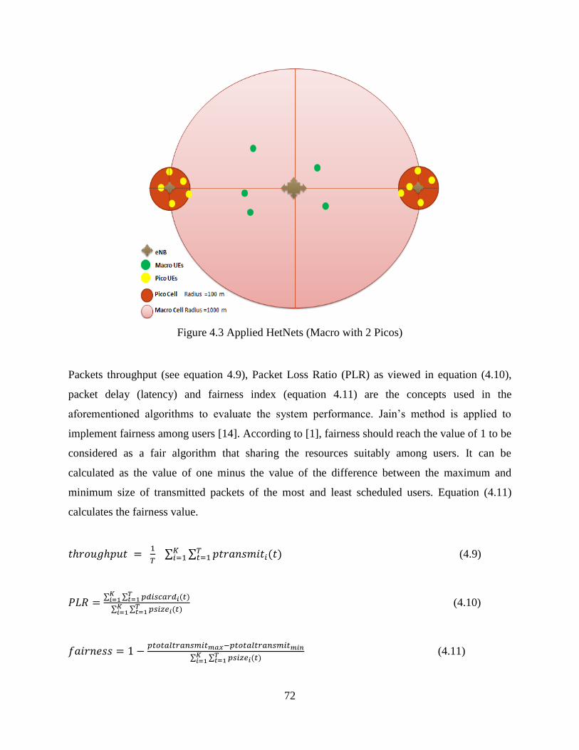
72

Figure 4.3 Applied HetNets (Macro with 2 Picos)

Packets throughput (see equation 4.9), Packet Loss Ratio (PLR) as viewed in equation (4.10),

packet delay (latency) and fairness index (equation 4.11) are the concepts used in the

aforementioned algorithms to evaluate the system performance. Jain’s method is applied to

implement fairness among users [14]. According to [1], fairness should reach the value of 1 to be

considered as a fair algorithm that sharing the resources suitably among users. It can be

calculated as the value of one minus the value of the difference between the maximum and

minimum size of transmitted packets of the most and least scheduled users. Equation (4.11)

calculates the fairness value.

(4.9)

(4.10)

(4.11)

73

Obviously, while is the size of transmitted packets, is the size

discarded or lost packets during the connection. is the summation of all arrived packets

that are buffered into serving eNB [1].

The aforementioned total size of transmitted packets of the best served UE and the worse served

UE are represented in equation (11) as and .Table 4.2

shows the entire system simulation parameters [1].

Parameters

Simulation time

Flow duration

30 s

20 s

Slot duration

TTI

Number of OFDM symbols/slot

Macro cell radius

Macro eNB Power

Pico cell radius

Pico eNB Power

0.5 ms

1 ms

7

1 km

49 dBm

0.1 km

30 dBm

User speed 3 km/h

VoIP bit rate 8.4 kbps

Video bit rate 242 kbps

Frame structure type FDD

Bandwidth 10 MHz

Number of RBs 50

Number of subcarriers 600

Number of subcarriers/RB 12

Subcarrier spacing 15 KHz

Table 4.2 LTE System Simulation Parameters

74

In order to get better results and confirm the outcomes, five simulations have been conducted for

each algorithm (PF, MLWDF and EXP) in each point of users (10, 20, 30, 40, 50, 60, 70 and 80).

This yields 120 simulations outcomes. The average values have been taken to draw the

simulation graphs at each point of users.

4.4.2. Simulation.1 Results

The system is judged base on throughput, Packet Loss Ratio (PLR), delay and fairness.

4.4.2.1. Throughput

The average overall system throughput is shown in Figure.4.4. Comparing the throughput for

“single Macro cell” for the same simulation parameters as viewed in Figure.4.5, the pico cells in

the scenario “Macro with 2 Picos” boost the throughput by adding gain that shown as an overall

system throughput increment for the same number of users. For instance, at 40 users using

MLWDF, the throughput is 25 Mbps for the scenario with 2 Picos while the Macro scenario is

only 9.3 Mbps. This is almost a double value. Further points show duple and triple throughput

values in the scenario of 2 Picos. However, the gain will reach a saturation level where no more

gain could be obtained due to the fact of limited radio resources availability while more users are

added to the system. Although MLWDF and EXP have almost similar behaviour in both

scenarios, a higher throughput is acquired in the 2 Pico case using both algorithms. It could note

that PF algorithm behaves better than the scenario of single Macro cell as seen Figure.4.5. PF is

developed for NRT traffic, but the simulation is for Video flows (RT traffic); hence, the other

simulated algorithms outperform PF.

Figure 4.4 Average System Throughput (Macro with 2 Picos)

75

Figure 4.5 Average System Throughput (single Macro cell)

4.4.2.2. Packet Loss Ratio (PLR)

PLR shown in the Figure.4.6 according to [15] is the packet loss ratio for a single Macro cell.

While the system is charged with more than 20 users, the PLR is increased for all experienced

algorithms taking into consideration that the PF is the worst case with the video traffic. Adding

two Picos to the previous system to create “Macro with 2 Picos” scenario enhances the PLR

while maintaining similar system behavior for all algorithms. Approximately, the PLR in Macro

with 2 Picos case is reduced to be a quarter of PLR value of single Macro cell scenario. For

example, at 70 users, MLWDF has 0.1 PLR value while for the same number of users MLWDF

has 0.5 PLR value in the single Macro scenario. PF algorithm is the worst case in both simulated

cases comparing with the other scheduling schemes. Figure.4.7 illustrates PLR for Macro with 2

Picos.

Figure 4.6 PLR of Video Flows (single Macro cell) [15]

76

Figure 4.7 PLR of Video Flows (Macro with 2 Picos)

4.4.2.3. Delay

According to [15] and as illustrated in Figure.4.8 , the delay in single Macro cell scenario is close

to be constant for PF, MLWDF and EXP/PF with value less than 5 ms while it suffers from rapid

increasing after 40 users for PF algorithm. If two Pico cells are added to the aforementioned

system, a similar performance is shown, but the delay value is decreased. In addition, the

threshold of PF is shifted at 60 users instead of 40 users in the single Macro case. To compare

MLWDF and EXP/PF in both scenarios, a certain point in Figures.4.8 and 4.9 could be

explained. For example at 60 users, in a single Macro cell the delay value is 50 ms while the

value is 20 ms in the Macro with 2 Picos. As a consequence, for MLWDF and EXP/PF, the delay

value with two Picos is approximately half the delay value without Pico cells. One of the

purposes of HetNets is to enhance the latency, and this is viewed in a practical simulation

illustrated in Figure.4.9. However, the delay manifests lower values (nearly 10 times lower) in

the scenario of the single cell with 2 Picos using PF scheme.

77

Figure 4.8 Packet Delay of Video Flows (single Macro cell)

Figure 4.9 Packet Delay of Video Flows (Macro with 2 Picos)

4.4.2.4. Fairness Index

When the number of users increases in single Macro cell more than 30, the fairness index of all

simulated algorithms is deviated down of the value “1”. At 40 users, PF experiments further

deviation close to value 0.8 compare with other algorithms that they are around 0.9 as seen in

Figure.4.10. The fairness index behaves similarly in the scenario of Macro with 2 Picos as shown

in Figure.4.11. However, the PF shows a minor different in which at 50 users it starts to decline

to get the value 0.8.

78

Figure 4.10 Fairness Index of Video Flows [15]

Figure 4.11 Fairness Index of Video Flows Macro with 2 Picos

4.5. Simulation.2-Single Macro Cell with two Pico Cells (Different Speed

Comparison)

This simulation has been done to compare between telecommunication systems that compromise

of a Macro cell with two small low power Pico cells where the users are moving in 3 Km/hand in

one scenario and 120 Km/h in the other scenario.

79


Similar simulation environment that have been mentioned in Simulation1 is applied in this

simulation. LTE-Sim platform is used with the added code that demonstrates the new scenario of

Macro with two Picos. The parameters in the Table 4.2 are applied, but the speed is changed to

be 120 Km/h instead of 3 Km/h. Similar Pico cells positions in the Macro cell as seen in

Figure.4.3 is considered. This distribution is more likely close to the normal Pico positions in the

practical networks, in which operators locate Pico cells in Macro boundary to extend the

coverage, increase capacity and boost the throughput. Useless Pico cells will be if their base

stations near the Macro eNB position, that is, the Macro eNB already serves the UE. Handover is

activated, and 3GPP urban Macro cell propagation loss model has been performed as

aforementioned in simulation1. Initially, each HetNets cell has a certain number of users who

can be handed over during the simulation between Macro and Picos and vice versa. In this

simulation, number of users increase equally in all cells. However, theoretically Pico cell could

serve 16-32 UEs simultaneously [17]. Each user has 50% video flows and 50% VoIP. The

outcomes are based on the video traffic.


It could predict the simulation results since high speed degrades the system behaviour the users’

connectivity with system’s cells will be worse. The degradation is shown as reducing overall

system throughput while increasing PLR, latency and fairness.

4.5.2.1. Throughput

As seen in Figure.4.12, the dashed lines denote PF, MLWDF and EXP/PF in the case of 120

Km/h speed. It is obvious that the system is degraded due to the speed increment for each user.

For example, the point 60 users has 16 Mbps throughput value if the mobility speed is 120 km/h

while in the case of 3 Km/h the same point has more than 25 Mbps for all scheduling schemes.

However, if it is compared with Figure.4.5 (throughput in Macro cell only at speed of 3 Km/h),

the system manifests better performance although the speed is 120 Km/h. This is due to the

positive impact of adding two Pico cells. As an example, the maximum throughput value viewed

in Figure.4.5 is almost 12 Mbps due to the effect that there are no Pico cells.

80


The PLR value is highly affected by the speed of mobility. Packets are likely to suffer of errors

and could be dropped while the speed is increased due to the fact that the connectivity with the

base stations gets worse. As seen in Figure.4.13, the PLR value is higher in the scenario of 120

Km/h speed, in which the higher PLR, the worse system performance. Considering point 60 of

users, the average PLR values for all scheduling algorithms is 0.33 while the speed is 120 Km/h.

Same point at speed 3 Km/h illustrates lower PLR values for all schedulers, for example, PLR of

PF is 0.14 which is almost half the value of 0.33 in the 120 Km/h scenario. The scheduling

schemes are performing similarly. However, MLWDF and EXP/PF outperform PF in both

scenarios.

Figure 4.12 Throughput of Video in Macro with 2 Picos

(3 Km/h and 120 Km/h speed)

Figure 4.13 PLR of Video in Macro with 2 Picos (3 Km/h and 120 Km/h speed)

81

4.5.2.3. Delay

Figure.4.14 shows the delay of the system in both when the speed is 120 Km/h (the dashed line)

and the speed 3 Km/h (the straight line). The delay is higher in the scenario of 120 Km/h

especially with the PF scheme. Maximum delay in the case of 3 Km/h is 20 ms as experimented

in this simulation.EXP/PF and MLWDF have similar behaviours in the both scenarios although

the delay in the case of 120 Km/h is almost double the value of that in the case of speed of

walking. For instance, at 60 users in the 120 Km/h speed, the EXP/PF and MLWDF has a delay

of 44 ms while in the other case the delay is 20 ms which is nearly half the value of 44 ms.


The system provides fairness values similar to those in the simulation1.Pf is outperformed by

MLWDF and EXP/PF where it shows more decline down the value of one as the number of

users increases. The speed has an impact on the fairness values. As it is seen in Figure.4.15, the

120 Km/h scenario enhances the fairness slightly than the 3 Km/h scenario for all scheduling

schemes. This gives a good indication that using HetNets (Macro with Pico cells) with high

speed mobility not only keeps the system performing similarly, but also could enhance the

fairness index. However, PLR, delay and throughput have lower values using high speed

mobility, thereby; the overall system is degraded when the users are moving fast.

Figure 4.14 Delay of Video in Macro with 2 Picos (3 Km/h and 120 Km/h speed)

82

Figure 4.15 Fairness Index in Macro with 2 Picos (3 Km/h and 120 Km/h speed)

4.6. Simulation.3- Single Macro Cell with Increasing Pico Cells

Third Simulation has been conducted to compare between different scenarios of a single Macro

cell telecommunication system by adding more Pico cells. The increment is constant; that is, in

each case two more Pico cells are added in new positions at the Macro cell edge.


Same simulation environment has been used for the rest of the study. However, further updated

code has been used in LTE-Sim simulation platform to perform this analysis. The simulation is

based on a scenario of a single Macro cell with 2, 4, 6, 8 and 10 small Pico cells. Each Pico

transmits 30 dBm of power while the Macro cell transmits 49 dBm. Table 4.2 parameters are set

up in all scenarios to maintain same values for the system while increasing the Pico cells by

factor of 2. This ensures that all new results of the system performance come through the factor

of adding Pico cells only. However, flow duration and simulation time have been modified to 30

and 40 respectively. All other aforementioned simulation environment elements are similarly

utilised such as 3GPP urban Macro cell path loss and handover activation. Users at Pico cells are

not equal to the Macro cell users. Pico cannot serve more than 30 users [17] users, thereby, after

30 users there are no more users could be added. Nevertheless, all cells start with 10 users and

increase by factor of 10. Flows are equally divided into Video and VoIP flows, in which each of

them is 50% of the total system traffics. In this simulation, there are two sides have to be

considered. One of them is increasing the number of Pico cell gradually by factor of 2, and the

other one is increasing the number of users by the factor of 10. Because of this, 3D graphs are

83

used to represent the system performance besides using 2D graphs to study the system behaviour

in different scheduling schemes. The distribution of the Pico cells within Macro boundary

follows Figure.4.16. Table 4.3 summarises the (x,y) values for each position from the simulation

outcomes.

Figure 4.16 Applied HetNets (Macro with Multiple Picos Scenarios)

Macro (x,y) 2 Pico cells

(x,y)

4 Pico cells(x,y) 6 Pico cells (x,y)

id 0, position: 0, 0

id 1, position:

1000, 0

id 2, position: -

999.9 , 1.5

id 1, position: 500.4, 865.7

id 2, position: -499, 866.5

id 3, position: -501.8, -

864.9

id 4, position: 497.6, -867.3


id 2, position: 500.4, 865.7

id 3, position: -499, 866.5

id 4, position: -999.9, 1.5

id 5, position: -501.8, -864.9

id 6, position: 497.6, -867.3

8 Pico cells(x,y) 10 Pico cells(x,y)


id 2, position: 707.3, 706.8

id 3, position: 0.79, 1000

id 4, position: -706.2, 707.9

id 5, position: -999.9, 1.5

id 6, position: -708.5, -705.6

id 7, position: -2.3, -999.9

id 8, position: 705.1 ,-709


id 2, position: 809.2, 587.5

id 3, position: 309.6, 950.8

id 4, position: -308.1, 951.3

id 5, position: -808.2, 588.8

id 6, position: -999.9, 1.5

id 7, position: -810.1, -586.2

id 8, position: -311.1, -950.3

id 9, position:

306.5, -951.8

id 10, position:

807.3, -590.1

Table 4.3 Pico Cells Positions in meters into the Macro Cell (Radius 1 Km)

84


As mentioned before, adding more Picos more likely enhances the system performance. This is

proven in this simulation demonstrated through the throughput, PLR, delay and fairness. Adding

2 extra Pico cell improves the overall system throughput with a certain value which cannot be

normalized .This is because number of reasons such as increasing the number of users,

increasing the effect of inter-cell interference while the number of users increases and simulation

parameters including power value, simulation time, flow duration affect that while the number of

users increases.

4.6.2.1. Throughput

The average overall system throughput for all scenarios is seen in Figure.4.17. Adding 2 Pico

cells provides almost constant gain in all applied scheduling schemes. To explain that, PF

algorithm (Table.4.4 in 5 cases) is taken as an example. Vertically, the number of users increases

by factor of 10, and by taking the cases (10 users) to (30 users) the gain value is 3.39 Mbps due

to UEs increments. For example, at 20 users the average value of for all scenarios is 6.78 Mbps

that equals the value of 3.39 at 10 users plus the 3.39 Mbps gain. The difference of average gain

between 30 users point and 20 users point is also 3.39 Mbps that proves adding 10 users

increases the throughput in constant value of the gain while adding 2 Pico cells to the system.

After 30 users, the Picos cannot serve more UEs, and the gain will continue at almost the same

value of the gain at 30 users, which is 10 Mbps as average. However, adding more users to the

system (only Macro users) boosts the throughput slightly with nearly 1 Mbps due to the effect of

scheduling algorithms only. Horizontally, moving up from 2 to 10 Pico scenarios the throughput

value increases by average gain of 10 Mbps. Figure.4.18 gives another view of the gain and

shows clearly the system performance in each case. All aforementioned values of the gain are not

constant, and they are based on the simulation parameters and system environment.

85

Figure 4.17 Throughput Gain of Video traffic in Macro with 2-10 Picos Scenarios

PF

Picos (Y-

axes)

Throughput(

Z-axes)

2 4 6 8 10 Average 2 Picos gain [Mbps]

10 5.09 8.48 11.88 15.28 18.67 3.39 Mbps increment

Users (X-

axes) 20 10.17 16.95 23.74 30.53 37.32 6.78 Mbps increment

30 15.124 25.21 35.36 45.46 55.64 10.13 Mbps increment

40 16.41 26.44 36.57 46.52 56.56 10.03 Mbps increment

50 17.26 27.11 36.93 47.05 57.19 9.98 Mbps increment

60 17.55 27.41 37.37 47.45 57.44 9.97 Mbps increment

70 17.29 27.14 37.35 47.46 57.80 10.12 Mbps increment

80 17.00 27.13 37.43 47.55 57.91 10.22 Mbps increment

Table 4.4 Throughput Gain Values and An Average of The Values

86

Figure.4.18 Throughput Gain of Video traffic in Macro with 2-10 Picos Scenarios


Although the number of users increases that means the PLR value increases accordingly, the

PLR values start getting down as the number of Pico cells raises. Adding more Picos can be

equivalent to the PLR increment due to more users is added to the system. For instance, PF

algorithm is the lower performance than other algorithms in most of the cases, in which the PLR

starts going up while the system is charged with more users. However, as seen in Figure.4.19 at

the 50 users, PF with 8 Pico cells case has the same PLR value of other schemes with 2 Pico

cells scenarios. This enforces the idea of equivalent; that is, adding more Picos enhances system

PLR of PF bringing it back to the value where other algorithms are in. Figure.4.20 gives 3D view

of the PLR behaviour in the dimension of adding more users and the dimension of adding more

Pico cells.

87

Figure 4.19 PLR Video traffic Comparison in Macro with 2-10 Picos Scenarios

Figure 4.20 PLR of Video traffic in Macro with 2-10 Picos Scenarios

88

4.6.2.3. Delay

Delay follows similar behaviour to the PLR. While the number of users increases, the delay gets

higher. Reverse of that, while Pico cells are added to the system, the delay becomes lower. Table

4.5 is an example of PF delay values that are obtained from the simulation to draw Figure.4.21

and 4.22. Similarly, MLWDF and EXP/PF have been drawn. PF has the higher delay values in

all scenarios and the highest value in the 2 Pico cell case while the number of users at the

maximum in this simulation. It is easily to notice that PF starts decreasing while the number of

Pico cells increases. Similar performance for all algorithms in all scenarios is viewed in

Figure.4.21. MLWDF and EXP/PF analogy the stairs, in which lower delay values are at 10 Pico

cells scenario climbing up to the higher at 2 Pico cells scenario.

Picos (Y-axes)

Delay

(Z-

axes) 2 4 6 8 10

10 6 5.8 5.64 5.53 5.56

Users

(X-

axes) 20 10.32 9.89 9.67 9.56 9.59

30 14.65 14.17 13.84 13.76 13.83

40 16.57 15.39 14.71 14.48 14.41

50 18.67 16.82 15.89 15.34 15.09

60 20.86 18.12 16.75 16.04 15.7

70 22.78 19.43 17.63 16.72 16.21

80 24.35 20.32 18.25 17.17 16.63

Table 4.5 PF Throughput Gain Values and An Average of The Values

89

Figure 4.21 Delay of Video traffic Comparison in Macro with 2-10 Picos Scenarios

Figure 4.22 Comparison Delay of Video traffic in Macro with 2-10 Picos Scenarios

90


The fairness index has to be closer to the value of one. Adding more users affects this value that

starts slope down. Figure.4.23 shows the fairness index of the system that has 2 to 10 Pico cells.

The value slightly declines from one for the MLWDF and EXP/PF while the PF suffers further

drop from the value of one. Adding more Pico cells has no effect on the fairness as shown from

the Figure.4.23 and Figure.4.24.Compare with the same system without Pico cells (as seen in

Figure.4.10), the system has similar behaviour although adding more cell slightly enhances the

overall system fairness value. From the values of all algorithms, the worst scenario of the

fairness index is at 8 Pico cells in which PF shows the lowest fairness value when the number of

users is 80 and the scenario is 8 Pico cells. MLWDF and EXP/PF also suffers further drop in the

same point as aforementioned in PF. Figure.4.24 illustrates that.

Figure 4.23 Fairness Index in Macro with 2-10 Picos Scenarios

91

4.7. Conclusion

This chapter investigates scheduling algorithms that are developed to enhance the LTE network

performance by sharing radio resources fairly among users utilizing all available resources.

These algorithms depend on traffic class and number of users, hence; different outcomes are

presented for each algorithm. To further boost the overall system performance, this study uses

heterogeneous networks concept by adding small cells (initially 2 Pico cells). This enhancement

is experienced through a throughput, PLR, delay and fairness. In the throughput the system gains

more data rate while in PLR the system suffers less packet loss values. Moreover, delay is

decreased and fairness stays similar. Approximately from the simulation1 outcomes, the overall

system performance is as follows: throughput is duplicated or nearly tripled relaying on the

number of users, the PLR is almost quartered, the delay is reduced 10 times (PF case) and

changed to be a half value (MLWDF/EXP cases), and the fairness stays closer to value of 1. On

the other hand, high speed mobility in simulation2 degrades the overall system performance

although the system appears better fairness index.

Figure 4.24 Fairness Index in Macro with 2-10 Picos Scenarios

92

Lastly, as the number of small cell increases as determined in simulation3, the system manifests

more enhancements as seen in 2D and 3D graphs for throughput, PLR, delay and fairness.

However, it is expected that a saturation state will be reached after a certain point of the number

of Pico cells and the number of users. The reason behind that is the inter-cell interference will

limit the performance since the same carrier frequency is used in all system’s cells. Considering

all scenarios, MLWDF manifests the best performance for video flows followed by EXP/PF.

Further enhancement could be applied in future papers such as almost blank subframes (ABS),

enhanced inter-cell interference cancelation (eICIC), cell range extension CRE concepts. and

using Carrier Aggregation (CA) and CoMP within HetNets.

References

[1] H. A. M. Ramli, R. Basukala, K. Sandrasegaran, and R. Patachaianand, "Performance of well known

packet scheduling algorithms in the downlink 3GPP LTE system," in Communications (MICC), 2009 IEEE

9th Malaysia International Conference on, 2009, pp. 815-820.

[2] Seung June Yi, S.C., Young Dae Lee, Sung Jun Park, Sung Hoon Jung 2012, Radio Protocols for LTE

and LTE-Advanced.

[3] [1] B. Liu, H. Tian, and L. Xu, "An efficient downlink packet scheduling algorithm for real time

traffics in LTE systems," in Consumer Communications and Networking Conference (CCNC), 2013 IEEE,

2013, pp. 364-369.

[4] A. Jalali, R. Padovani, and R. Pankaj, "Data throughput of CDMA-HDR a high efficiency-high data rate

personal communication wireless system," in Vehicular Technology Conference Proceedings, 2000. VTC

2000-Spring Tokyo. 2000 IEEE 51st, 2000, pp. 1854-1858.

[5] M. Andrews, K. Kumaran, K. Ramanan, A. Stolyar, P. Whiting, and R. Vijayakumar, "Providing quality of

service over a shared wireless link," Communications Magazine, IEEE, vol. 39, pp. 150-154, 2001.

[6] J.-H. Rhee, J. M. Holtzman, and D. K. Kim, "Performance analysis of the adaptive EXP/PF channel

scheduler in an AMC/TDM system," Communications Letters, IEEE, vol. 8, pp. 497-499, 2004.

[7] J. Zyren and W. McCoy, "Overview of the 3GPP long term evolution physical layer," Freescale

Semiconductor, Inc., white paper, 2007.

[8] B. Riyaj, M. R. H. Adibah, and S. Kumbesan, "Performance analysis of EXP/PF and M-LWDF in

downlink 3GPP LTE system," 2009.

[9] X. Qiu and K. Chawla, "On the performance of adaptive modulation in cellular systems," Communications,

IEEE Transactions on, vol. 47, pp. 884-895, 1999.

[10] S. C. Nguyen, K. Sandrasegaran, and F. M. J. Madani, "Modeling and simulation of packet scheduling in

the downlink LTE-advanced," in Communications (APCC), 2011 17th Asia-Pacific Conference on, 2011,

pp. 53-57.

[11] A. Alfayly, I.-H. Mkwawa, L. Sun, and E. Ifeachor, "QoE-based performance evaluation of scheduling

algorithms over LTE," in Globecom Workshops (GC Wkshps), 2012 IEEE, 2012, pp. 1362-1366.

93

[12] G. Piro, L. A. Grieco, G. Boggia, F. Capozzi, and P. Camarda, "Simulating LTE cellular systems: an open-

source framework," Vehicular Technology, IEEE Transactions on, vol. 60, pp. 498-513, 2011.

[13] M. Iturralde, T. Ali Yahiya, A. Wei, and A. Beylot, "Resource allocation using shapley value in LTE

networks," in Personal Indoor and Mobile Radio Communications (PIMRC), 2011 IEEE 22nd International

Symposium on, 2011, pp. 31-35.

[14] R. Jain, D.-M. Chiu, and W. R. Hawe, A quantitative measure of fairness and discrimination for resource

allocation in shared computer system: Eastern Research Laboratory, Digital Equipment Corporation, 1984.

[15] AL-Jaradat, Huthaifa 2013, ‘On the Performance of PF, MLWDF and EXP/PF algorithms in LTE’.

[16] Holma H, Toskala A 2012, “LTE-Advanced 3GPP Solution for IMT-Advanced”.

[17] Hu, Rose Qingyang Qian, Yi 2013, ‘Comparison Femto cell and Pico cell key features”, Heterogeneous

Cellular Networks (2nd Edition).

1

Research Proposal

LTE-Advance

Enhancement Using CA and CoMP within

HetNets

By

Haider Al Kim

November 2014

Supervisor: Dr. Kumbesan Sandrasegaran

2

Introduction

The telecommunication networks have rapidly been updated since 1980’s where 1G of mobile

telecommunication was proposed. Low traffic capacity, poor call quality and higher power usage

are characteristics of 1G network. Available network resources have to be utilized efficiently to

increase cell capacity, coverage and satisfy Quality of service QoS requirements. Most recent

trends of researchers are designing models that can meet users’ expectations. Although modern

networks have been designed carefully to fulfill the requirements needed by the end users;

significant challenges have emerged. There is a limited bandwidth that has to be used

sufficiently. RRM and air interface techniques have become the research interest fields for the

researchers.

3

Contents

Mobile Telecommunications Trends

Technology Review

Focus Area

Statement of the problem

Methodology

Research Timeline

Bibliography

4

Mobile Telecommunications Trends

Mobile networks have already grown rapidly passing some remarkable signs. Rapid computer

technologies have led to short-period mobile evolution which is aimed to meet the increment of

higher data rate requirements and satisfy a certain agreed QoS. This emulation is shown in

Figure.1.3GPP standardizes the most important demands that have to be met in order to cross the

mobile system to the new generation that is 4G. 4G fulfills the IMT-Advance constraints which

are agreed to increase the user expectation. At the top of the hierarchy, LTE-A, a subset of Rel-

10, has been proposed with significant challenges. The term LTE-A also refers to 4G although

informally the term 4G is used for WiMAXTM.4G is commercially used as a term by some

operators to describe HSPA evolution. International Telecommunications Union Radio

communication Sector (ITU-R) has involved in the development of the proposed system by

3GPP introducing the Release 10 or what so-called recently LTE-A. The ITU-R involvement in

specifying the LTE-A requirements has complicated the process of setting up Rel-10. Although

Rel-8 could meet most of the 4G requirements, LTE-A has other features that could not be

satisfied by LTE. These LTE-A-based requirements are higher bandwidth coming from carriers

aggregating (CA), and higher efficiency could be conducted using higher uplink multiple access

technologies and enhanced multi-in-multi-out MIMO antennas. Further enhancements could be

as essential parts of LTE-A network, but they do not have to be LTE-A requirements. These

features are:

- Support for heterogeneous networks (HetNets) and Relaying

- Coordinated multipoint transmission/reception (CoMP)

- LTE self-optimizing network (SON) enhancements

- Mobility enhancements for Home enhanced-node-B (HeNB)

- RF requirements for fixed wireless customer premises equipment (CPE)

5

Figure.1 Wireless evolution 1990–2012 and beyond: www.low-powerdesign.com

Technology Review

Different access technologies have been introduced with each mobile generation network trying

to address the problems in the previous versions. FDMA network that is an access method used

in the first generation of the mobile telecom-systems has been modified presenting what so-

called orthogonal FDMA that is adopted to be applied in the new mobile generations.

Technically, FDMA is a divided available system bandwidth into non-overlapping frequencies.

The main usage of FDMA was for analogue systems that have been changed later to modern

digitized systems. For the second generation 2G, TDMA is applied as an access technology. That

is; the division is based on the time intervals for each call. Analogue-to-digital converters are

used in TDMA to produce digital signals constructing consolidated digital stream that can be

carried on a single radio channel. While the telecommunication systems continued development,

modern access methods have been adopted. CDMA is the new access technique that is used with

3rd

generation (3G). It is considered a very efficient method to avoid overlapping of FDMA and

the limitation of the time interval of TDMA. Using the code to separate between conversations is

what CDMA has brought. More data rate is required in the recent days due to the demand of

high-resolution video streams and high-quality voice conversations.3GPP provided the standards

of long-term evaluation system LTE. LTE uses most recent technologies in mobile networks.

http://www.low-powerdesign.com/

6

One of them is Orthogonal Frequency Division Multiple Access technology OFDMA that is

utilized mainly to minimize interference effect for overlapped frequencies. Another technology is

MIMO that plays a major role in the LTE system performance that further enhanced to propose

advanced MIMO. LTE with these technologies provides higher efficiency of the spectrum, lower

delay and seamless handover, thereby, performs better than the previous systems.

OFDMA: it is one of a key element in LTE network which is basically used to robust the

resistance to multipath fading and interference as well as it is considered as a digital signal

processing techniques. It guarantees little updating to the existed air interface while flexible

deploying over available frequencies. It also provides an average value of the inter-cell

interference caused by neighboring cells and an average value for intra-cell interference caused

by overlapped frequencies. By spreading the carriers over the available spectrum, OFDMA

provides frequency diversity and excellent coverage. It uses large, narrow band (180 kHz) sub-

carriers for multi-carrier transmission to carry data. Figure.2 shows the basic LTE downlink

physical resource where OFDM symbols are grouped into resource blocks.

Figure.2 Basic LTE downlink physical resource using OFDMA: www.tutorialspoint.com

- MIMO/Advanced MIMO: it is antenna structure that is adopted to robust the data rate

and maximize the performance in LTE-A. The expected LTE-A MIMO is 8x8 downlink

antenna configuration while (4x4) antenna configuration is proposed to be utilized in the

uplink direction. It is one of the suggested smart antenna technologies. The significant

benefit of MIMO is that it provides higher data rate without the need to increase the

http://www.tutorialspoint.com/

7

bandwidth or the transmission power. This can be conducted by spreading the used power

of the transmission among the antennas to enhance the spectral efficiency by obtaining

array gain.

- Relaying and Heterogeneous networks (Macro with Pico or Femto cells): relay, Pico and

Femto are small low power nodes that inserted within or on the edge of the large mobile

cells to enhance the throughput and increase the capacity and coverage. A relay is slightly

different since it protocol structure recently reaches layer 3 (router more than to be a

repeater only). However, the main purpose of it is that retransmitting the received signal

without modifying to the far end that it is out of the main coverage area of large cell.

Small cells and relay are considered an effective air interface enhancement methods

which require lower cost and little modifying to the existing mobile networks.

- Carrier Aggregation CA: in LTE, single carrier is allocated to the LTE user. When LTE-

A is proposed, the demand for more data rate that has to be provided to the LTE-A user is

studied. Hence, CA is applied to increase the bandwidth, thereby, it increases the bit rate.

On the other hand, backward compatibility exists with legacy schemes Rel8/9 that means

they can co-exist with LTE-A where the CA is based on Rel8/9 carrier component. The

maximum LTE available bandwidth is 20 MHz. By aggregating 5 of 20 MHz, the new

LTE-A bandwidth is 100 MHz that provides a higher rate of throughput. Recent studies

are proposed different algorithms to aggregate carrier in LTE-A based on that if the

carriers are on the same frequency band (contiguous or non- contiguous) or cross-carrier

frequency (non- contiguous only).

- Coordinated Multi-Point (CoMP) Transmission/Reception is a mechanism, in which a

number of geographically separated eNBs are cooperated to serve one user in the network

in order to improve the performance the users in the covered areas. The suggested

method of connecting these eNBs is using high speed dedicated connections, for

example, microwave links or optical fiber. The inter-cell interference impact is

affirmatively minimized using CoMP in both the downlink and uplink directions [4].

8

Focus Area

Deploying Heterogeneous networks (HetNets) approach is one of the probable

key features of future LTE-A networks. There are different methods to apply

HetNets in wireless systems. Using separate frequency band in a small cell from

the frequency in a large cell is to avoid the interference. This method is call

dedicated carrier HetNets. There is a drawback of using dedicated carrier, in

which the probability of inefficient usage of the frequency band exists. Moreover,

intra-frequency handover is required while the user is moving between HetNets

cells. The most common approach of HetNets (Macro with small cells) is

applying the same frequency band in all cells with HetNets. This increases the

inter-cell interference, but it could introduce higher spectral efficiency. However,

careful interworking between HetNets cells is vital in the scenario of using the

same frequency in all HetNets cells. That is; it requires a centralized node to

control the HetNets cells, which is called Remote Radio Heads (RRH). According

to NTT DoCoMo [5], new base station is proposed that using advanced

centralized Radio Access Network structure. Once this centralized architecture is

deployed using multiple bands, it is possible to use carrier aggregation in Rel-10

as an extension of a base station. CA could combine contagious or non-

contiguous frequency bands to create LTE required bandwidth. Normally, CA is

conducted on the same cell using the available carriers. However, CA is enhanced

to be involved within multi-cells using the centralized node. With HetNets, a

small eNB has been introduced as a low-cost base station with a reduced

transmission power. Rel-11 provided a multi-carrier aggregation using the timing

advance enhanced uplink power control [6]. Figure.3 illustrates HetNets with

primary cell (large-Macro cell) and secondary cell (small–Pico or Femto). In this

scenario, the Large cell is responsible for providing control signaling, system

information and limited data transmission while the small cell is responsible for

providing the required high data rate. It is beneficial in both cases, CA with

dedicated frequency or co-channel. Due to some drawbacks of this CA in HetNets

such as users’ terminal compatibility a with multi-carrier aggregation of Multiple

9

Timing Advance, another method that does not depend on the centralized node

can be used. That is, large and small cells can operate with own control signaling

for both layered frequencies. This approach requires enhanced interference

management such as ICIC. However, ICIC is limited to the PDSCH data;

therefore, it requires new solutions to separate the control channels. PDCCH is

used to provide full control channel protection especially if it is used as cross-

carrier scheduling. In this case, the interference will be at its minimum value if the

small cell does not use the PDCCH. Figure.4 shows the concept of using PDCCH

in co-channel HetNets.

Figure.3 Multi-Carrier Aggregation in LTE-A HetNets [6]

Figure.4 CA in co-channel scenario in LTE-A HetNets [6]

10

Statement of the problem

Compare with Time Domain Interference Coordination using ABS (Almost Blank

subframe) in eICIC, the aforementioned Frequency Domain Interference

Coordination using PDCCH cross-carrier scheduling has some benefits. Using

eICIC introduces more complexity in the network, for example, signaling and

measurements are more likely to be higher in a co-channel deployment.

However, there is a probability that Macro cell passes out the PDCCH since it

uses cross-carrier scheduling. Moreover, to support MIMO, enhanced PDCCH is

required (ePDCCH) that is already addressed in 3GPP Rel-11 [6].

The current deployment of small cell and relays is using the ideal backhaul which

depends on a centralized architecture and supports easily CA and CoMP

operations [4]. Studies are proposed new methods of deploying small cell with

non-ideal backhaul. Currently in Rel-11, it could aggregate two TDD carriers with

different configuration of uplink and downlink. Such configuration requires UE

has an ability to transmit and receive in parallel. This could lead to that such

system is similar to FDD. Hence, operators could combine FDD and TDD

spectrums in one solution. For HetNets, a clustered TDD small cell deployment

could be possible as shown in Figure.5. By separating these clusters, a dynamic

adjacent of uplink / downlink frame structure could be possible relying on the

need of local traffic in the small cells.

11

Figure.5 Dynamic TDD in LTE-A HetNets [6]

Using HetNet with CA and CoMP is the key evolution of future networks.

Investigating using HetNets small cell as corporative cells to apply CA and CoMP

techniques is a major interest in this proposal. Intensive most recent papers will be

reviewed and studied that address and discuss the current challenges as motioned

before ideal backhaul as a centralized architecture where CA and CoMP rely on.

Figure.6 shows the suggested scenario for future HetNets. Hence, HetNets

deployment not only supports large cell to serve some users who suffer from bad

connectivity with Macro cell, but also could be utilized simultaneously as

corporative cells to apply CA and CoMP concept. It could further increase

throughput, coverage and capacity besides reducing the latency.

More enhancements for small cell will be considered, such as using 256 QAM to

enhance spectral efficiency, enhanced inter-frequency measurement and enhance

interference coordination to improve small cell operation [6].

12

Figure.6 CA with ideal and non-ideal backhaul in the suggested HetNets [6]

13

Methodology

Technology Review Searching State of the art scientific

papers

Identifying existed problem/Technology limitation

Preparing developing model/writing paper

Code writing and Simulation implementation

Results/ Conclusions

Writing Thesis

14

Research Timeline

Task First Year Second Year Third Year Forth Year

1st Semester

2nd Semester

3rd Semester

4th Semester

5th Semester

6th Semester

7th Semester

8th Semester

Technology Review Searching State of

the art scientific papers

Identifying existed problem/Technology limitation

Preparing developing model/writing paper

Code writing and Simulation implementation

Results/ Conclusions

Writing Thesis /Extension if required

15

Bibliography

[1] A. T. Moray Rumney, LTE and the Evolution to 4G Wireless: Design and

Measurement Challenges, Second Edition. John Wiley and Sons, Ltd, 2013.

[2] A. Toskala and H. Holma, WCDMA for UMTS HSPA Evolution and LTE,

Fourth Edition. John Wiley and Sons, Ltd, 2007.

[3] D. K. Sandrasegaran, \Lecture note, lte radio resource management," tech.

rep., University of Technology, Sydney.

[4] I. F. Akyildiz, D. M. Gutierrez-Estevez, and E. C. Reyes, "The evolution to

4G cellular systems: LTE-Advanced," Physical Communication, vol. 3, pp. 217-

244, 2010.

[5] Press Release NTT DoCoMo TOKYO, JAPAN, February 21, 2013:

“DOCOMO to Develop Next generation Base Stations Utilizing Advanced C-

RAN Architecture for LTE-Advanced”

[6] Eiko Seidel, “LTE-A HetNets using Carrier Aggregation” , NoMoR Research

GmbH, Munich, Germany, June 2013.

Appendix

- LTE-Sim Macro with Pico Applied Code

- Published Paper (IJWMN)

1

APPLIED CODE

1- Simulations Parameters

Type (Shell Code, .sh)

2- Simulations Parameters

Type (C++, .h)

2

3- Single Macro with Multiple Pico Cells - Cells Positions Part of

the Code

Type (C++, .h)

4- Single Macro with Multiple Pico Cells – Create Pico Cells Part

of the Code

Type (C++, .h)

3

5- Main LTE-Sim Execution File includes Single Macro with

Multi Pico Passing Parameters from the (.sh) file (C++ , .cpp)

6- An Example of The First Part of Simulation File Outcomes

International Journal of Wireless & Mobile Networks (IJWMN) Vol. 6, No. 5, October 2014

DOI : 10.5121/ijwmn.2014.6509 109

MACRO WITH PICO CELLS (HETNETS) SYSTEM

BEHAVIOUR USING WELL-KNOWN SCHEDULING

ALGORITHMS

Haider Al Kim1, Shouman Barua2, Pantha Ghosal2 and Kumbesan Sandrasegaran2

1Faculty of Engineering and Information Technology, University of Technology Sydney,

Australia {Haider.A.AlKim}[email protected]

{shouman.barua, pantha.ghosal, kumbesan.sandrasegaran}[email protected]

Abstract

This paper demonstrates the concept of using Heterogeneous networks (HetNets) to improve Long Term

Evolution (LTE) system by introducing the LTE Advance (LTE-A). The type of HetNets that has been chosen for

this study is Macro with Pico cells. Comparing the system performance with and without Pico cells has clearly

illustrated using three well-known scheduling algorithms (Proportional Fair PF, Maximum Largest Weighted

Delay First MLWDF and Exponential/Proportional Fair EXP/PF). The system is judged based on throughput,

Packet Loss Ratio PLR, delay and fairness.. A simulation platform called LTE-Sim has been used to collect the

data and produce the paper’s outcomes and graphs. The results prove that adding Pico cells enhances the

overall system performance. From the simulation outcomes, the overall system performance is as follows:

throughput is duplicated or tripled based on the number of users, the PLR is almost quartered, the delay is

nearly reduced ten times (PF case) and changed to be a half (MLWDF/EXP cases), and the fairness stays

closer to value of 1. It is considered an efficient and cost effective way to increase the throughput, coverage

and reduce the latency.

Keywords

HetNets, LTE &LTE-A, Macro, Pico, Scheduling algorithms & LTE-Sim

1. INTRODUCTION

In the Long Term Evolution so-called LTE, the requirements for larger coverage area, more capacity,

and high data rate and low latency have led to search for cost-effective solutions to meet these

demands. Hence, the development in the telecommunication networks has adopted different

directions to enhance the LTE system taking into account the International Mobile

Telecommunications (IMT-2000) standards that have to be satisfied [1]. Network-based technologies

such as Multiple Input and Multiple Output MIMO/ advanced MIMO and Transmission/Reception

Coordinated Multi-Point CoMP are LTE enhancements that introduce LTE Advance (LTE-A). Other

less cost enhancements based on air interfaces are proposed, such as improving spectral efficiency

involving using Heterogeneous networks (HetNets). HetNets are small and less power cells within

the main macro cells with different access technologies to close up the network to the end users and

increase their expectation [16].According to [2], there are two main practical HetNets classes: Macro

with Femto and Macro with Pico. Femto and Pico are the small and less power cells. To save the

cost, operators use the same carrier frequency in the large and small cells which, on the other hand,

proposes interference challenges. Figure 1 gives the main concept of HetNets. To clarify, user in LTE

is well-known as a UE.

mailto:%7bHaider.A.AlKim%[email protected]

mailto:%7bshouman.barua,%20pantha.ghosal,%20kumbesan.sandrasegaran%[email protected]


110

Figure.1 an example of HetNets

In LTE and LTE-A, the element that is responsible for Radio Resources Management (RRM) is

enhanced Node Base station (so-called eNB). The eNB does all required management including

Packet Scheduling (PS) which is the focus in the paper. PS can guarantee the agreed quality of

service demands (QoS) because it is responsible for the best and effective utilizing of the affordable

radio resources and in charge of data packets transmission of the users[3].

3rd Generation Partnership Project (3GPP) has left the scheduling algorithms to be vendor specific

according to user’s requirements and network capability. Therefore, various PS algorithms have

been proposed depending on the traffic sorts and provided services. PF, MLWDF and EXP/PF

algorithms [4][5][6] are used in this paper to study and compare between the system behaviours in

HetNets (single Macro with 2 Pico cells) using these three types of algorithms. Scheduling

algorithms ensure that QoS requirements have been met. This can be conducted by prioritizing each

link between the eNB and the users, the higher priority connection the first handled in the eNB.

This paper is organized as follows. Section II discusses the downlink system model of LTE. The

followed section (III) describes in more details packet scheduling algorithms, while Section IV

present simulation environment. Section V shows the outcomes of the simulation. Finally, conclusion

is given in Section VI.

2. DOWNLINK SYSTEM MODEL OF LTE

The basic element in the downlink direction of the LTE networks is called Resource Block

(RB).Each UE is allocated certain number of resource blocks according to its status, the traffic type

and QoS requirements. It could define the RB in both frequency domain and time domain. In the time

domain, it comprises single (0.5 ms) time slot involving 7 symbols of OFDMA (orthogonal

frequency division multiple access). In the frequency domain, on the other hand, it consists of twelve

15 kHz contiguous subcarriers resulting in 180 kHz as a total RB bandwidth [7].

As aforementioned before, the eNB is responsible for PS and other RRM mechanisms. The

bandwidth that is used in this study is 10 MHz considering the inter-cell interference is existed. The

period that eNB performs new packet scheduling operation is the Transmission Time Interval (TTI).


111

TTI is 1 ms that mean the users are allocated 2 contiguous radio resource blocks (2RBs). The

scheduling decision in the serving eNB is made based on the uplink direction reports come from the

UEs at each transmission time interval. The reports comprise the channel conditions on each RB,

such as signal to noise ratio (SNR). The serving eNB uses the SNR value involved in the reports to

specify the DL data rate for each served UE in each TTI. For example, how many bits per 2

contiguous RBs [8].

The data rate for user i at j sub-carrier on RB and at t time can be determined by using equation

(1) as proposed in [9].

(1)

A =

B =

C =

D = rgg

The number of bits per symbol is “A”. The number of symbols per slot is “B”. While “C” represents

how many slots per TTI, “D” clarifies how many sub-carriers per RB. Table 1 summarizes the

mapping between SNR values and their associated data rates.

Table 1. Mapping between instantaneous downlink SNR and data rate

Minimum SNR Modulation and Data Rate Level (dB) coding (Kbps) 1.7 QPSK (1/2) 168 3.7 QPSK (2/3) 224 4.5 QPSK (3/4) 252 7.2 16 QAM (1/2) 336 9.5 16 QAM (2/3) 448 10.7 16 QAM (3/4) 504 14.8 64 QAM (2/3) 672 16.1 64 QAM (3/4) 756

Upon the packets reach the eNB, they are buffered in eNB in a specific container allocated for each

active UE. Moreover, the buffered packets are assigned a time stamp to ensure that they will be

scheduled or dropped before the scheduling time interval is expired, and then using First-In-First-Out

(FIFO) method they are transmitted to the users in the downlink direction. To explain the scheduling

operation, PS manager (is a part of eNB functionalities) at each TTI priorities and classifies the

arriving users’ packets according to preconfigured scheduling algorithm.

Scheduling decision is made based on different scheduling criteria that have been used in various

algorithms. For example channel condition, service type, Head-of-Line (HOL) packet delay, buffer

status, and so on so forth. One or more RBs could be allocated to the selected user for transmission

with the highest priority. Figure 2 shows the packet scheduler in the downlink direction at eNB.


112

Figure.2 Downlink Packet Scheduler of the 3GPP LTE System [10]

3. PACKET SCHEDULLING ALGORITHMS

The efficient radio resource utilization and ensuring fairness among connected users, as well as

satisfying QoS requirements, are the main purposes of using PS algorithms [11].The PS algorithms

that have been used in this study are : Proportional Fair (PF) algorithm, Maximum-Largest Weighted

Delay First (MLWDF or ML) and the Exponential/Proportional Fair (EXP/PF or EXP) algorithm. It

should be noted that these algorithms are used.

3.1. Proportional Fair (PF) Algorithm

For non-real time traffic, the PF was proposed which is used in a Code Division Multiple Access-

High Data Rate (CDMA-HDR) system in order to support Non-Real Time (NRT) traffic. In this

algorithm, the trade-off between fairness among users and the total system throughput is presented.

This is, before allocating RBs, it considers the conditions of the channel and the past data rate.

Any scheduled user in PF algorithm is assigned radio resources if it maximizes the metric k that

calculated as the ratio of reachable data rate of user i at time t and average data rate of the

same user at the same time interval t:

(2)

where;

(3)

is the window size used to update the past data rates values in which the PF algorithm maximizes

the fairness and throughput for any scheduled user. Unless user i is selected for transmission

at , = 0.


113

3.2. Maximum Largest Weighted Delay First (MLWDF) Algorithm

If the traffic is a Real Time (RT), the MLWDF is introduced which is used in CDMA-HDR system in

order to support RT data users [11].It is more complex algorithms compare with PF and is used in

different QoS user’s requirements. This is because it takes into account variations of the channel

when assigning RBs. Moreover, if a video traffic scenario, it takes into consideration time delay. Any

user in MLWDF is granted RBs if it maximizes the equation below:

(4)

where;

(5)

where is a difference in time between current and arrival times of the packet that known as the

Head Of Line (HOL) packet delay of user i at time t.

Similarly to PF equation, while the achievable data rate of user i at time t is , the average data

rate of the same user at the same time interval t is . and are the delay threshold for a

packet of user i and the maximum HOL packet delay probability of user i respectively. The later is

considered to exceed the delay threshold of user i.

3.3. Exponential/Proportional Fair (EXP/PF) Algorithm

Since PF is not designed for multimedia applications (only for NRT traffic), an enhanced PF called

EXP/PF algorithm was proposed in the Adaptive Modulation and Coding and Time Division

Multiplexing (AMC/TDM) systems. The EXP/PF algorithm is designed for NRT service or RT

service (different sorts of services). The metric is used for both RT nad Non-RT in which RBs are

assigned to users based on .

(6)

where,

(7)

(8)

where the average number of packets at the buffer of the eNB at time t is represented by , k and

in equation (8) are constants, is explained in MLWDF, is the HOL packets delay of

RT service and is the maximum delay of RT service users. The EXP/PF differentiates between

RT and NRT by prioritizing RT traffic users over the NRT traffic users if their HOL values are

reaching the delay threshold.


114

4. SIMULATION ENVIRONMENT

LTE-Sim simulator is used in this paper to do the entire analysis and study [12]. The most recent

version of LTE-Sim (version 5) has not involved yet any code regarding the HetNets type (Macro with

Pico cells). The developed code used in this paper could be considered as an enhancement of the

released LTE-Sim versions. However, LTE-Sim has a detailed code (or what authors are named it:

scenario) which can be used to simulate and examine HetNets type (Macro with Femto). Our paper is

based on a scenario of a single Macro cell with 2 small Pico cells that are reduced their powers. More

Picos can be added to the system, and enhanced system behaviour will be presented. However,

according to [2], while the number of Pico cells is increased, more inter-cell interference is

experienced since the same carrier frequency is used in each cell (Macro and Picos).

Figure 3 shows the entire system that is used in this paper: Macro cell of 1 km and 2 Pico cells of 0.1

km located on the Macro edge. This design is chosen to analog a real system aimed to cover larger

area and more users, especially the users in the cell edge where they suffer from lack of connectivity

with Macro cell. The inter-cell interference is modeled. Video and VoIP traffic are used to represent

user’s data. Each user has 50 % Video traffic and 50% VoIP flows.

Handover is activated. Each cell starts a certain number of users. Non-uniform user distribution

within the cells is applied and 3km/h constant speed is utilized as the mobility user speed. In

addition, the 3GPP urban Macro cell propagation loss model has been implemented including path-loss,

penetration loss, multi-path loss and shadow fading which are summarized below [13]:

Pathloss: , d refers the distance between the eNB and the user in

kilometers.

Penetration loss: 10 dB

Multipath loss: using one of the well-known methods called Jakes model

Shadow fading loss (recently it could be used as a gain in LTE-A): log-normal distribution

- Mean value of 0 dB.

- Standard deviation of 10 dB.

Figure.3 Applied HetNets (Macro with 2 Picos)


115

Packets throughput (see equation 9), Packet Loss Ratio (PLR) as shown in equation 10, packet delay

(latency) and fairness index (equation 11) are the concepts used in the aforementioned algorithms to

evaluate the system performance. Jain’s method is applied to implement fairness among users [14].

According to [1], fairness should reach the value of 1 to be considered as a fair algorithm that sharing

the resources suitably among users. It can be calculated as value 1 minus the value of the difference

between the maximum and minimum size of transmitted packets of the most and least scheduled

users. Equation (11) calculates the fairness value.

(11)

Obviously, while is the size of transmitted packets, is the size discarded

or lost packets during the connection. is the summation of all arrived packets that are buffered

into serving eNB [1].

The aforementioned total size of transmitted packets of the best served UE and the worse served UE

are represented in equation (11) as and .

Table 2 shows the entire system simulation parameters [1].

Table 2. LTE system simulation parameters

Parameters

Simulation time

Flow duration

30 s

20 s

Slot duration

TTI

Number of OFDM symbols/slot

Macro cell radius

Macro eNB Power

Pico cell radius

Pico eNB Power

0.5 ms

1 ms

7

1 km

49 dBm

0.1 km

30 dBm

User speed 3 km/h

VoIP bit rate 8.4 kbps

Video bit rate 242 kbps

Frame structure type FDD

Bandwidth 10 MHz

Number of RBs 50

Number of subcarriers 600

Number of subcarriers/RB 12

Subcarrier spacing 15 KHz


116

In order to get better results and to confirm the outcomes, five simulations have been conducted for

each algorithm (PF, MLWDF and EXP) in each point of users (10, 20, 30, 40, 50, 60, 70 and 80).

This yields 120 simulations outcomes. The average values have been taken to draw the simulation

graphs at each point of users.

5. SIMULATION RESULTS

The average overall system throughput is shown in figure 4. Comparing the throughput for “single

Macro cell” for the same simulation parameters as shown in figure 5, the pico cells in the scenario

“Macro with 2 Picos” boost the throughput by adding gain that shown as an overall system

throughput increment for the same number of users. For instance, at 40 users using MLWDF, the

throughput is 25 Mbps for the scenario with 2 Picos while the Macro scenario is only 9.3 Mbps. This

is almost a duple value. Further points show duple and triple throughput values in the scenario of 2

Picos. However, the gain will reach a saturation level where no more gain could be shown due to the

fact of limited radio resources availability while more users are added to the system. Although

MLWDF and EXP have almost similar behaviour in both scenarios, a higher throughput is shown in

the 2 Pico case using both algorithms. It could note that PF algorithm as shown figure 5 behaves

better than the scenario of single Macro cell. PF is developed for NRT traffic, but the simulation is

for Video flows (RT traffic); hence, the other simulated algorithms outperform PF.

PLR shown in the figure 6 according to [15] is the packet loss ratio for a single Macro cell. While the

system is charged with more than 20 users, the PLR is increased for all experienced algorithms

taking into consideration that the PF is the worst case with the video traffic. Adding two Picos to the

previous system to create “Macro with 2 Picos” scenario enhances the PLR while maintaining similar

system behavior for all algorithms. Approximately, the PLR in Macro with 2 Picos case is reduced to

be a quarter of PLR value of single Macro cell scenario. For example, at 70 users, MLWDF has 0.1

PLR value while for the same number of users MLWDF has 0.5 PLR value in the single Macro

scenario. Comparing between scheduling schemes, the worst case is the PF algorithm in both cases.

Figure 7 illustrates PLR for Macro with 2 Picos.

According to [15] and as shown in figure 8 , the delay in single Macro cell scenario is close to be

constant for PF, MLWDF and EXP/PF with value less than 5 ms while it suffers from rapid

increasing after 40 users for PF algorithm. If two Pico cells are added to the aforementioned system,

a similar performance is shown, but the delay value is decreased. In addition, the threshold of PF is

shifted at 60 users instead of 40 users in the single Macro case. To compare MLWDF and EXP/PF in

both scenarios, a certain point in figures 8 and 9 could be explained. For example at 60 users, in a

single Macro cell the delay value is 50 ms while in the Macro with 2 Picos the value is 20 ms. As a

consequence, for MLWDF and EXP/PF, the delay value with two Picos is approximately half the

delay value without Pico cells. One of the purposes of HetNets is to enhance the latency, and this is

shown in a practical simulation illustrated in figure 9. However, the delay shows lower values (nearly

10 times lower) in the scenario of single cell with 2 Picos using PF scheme.

When the number of users increases in single Macro cell more than 30, the fairness index of all

simulated algorithms is deviated down of the value “1”. At 40 users, PF shows further deviation

close to value 0.8 compare with other algorithms which they are around 0.9. The fairness index

behaves similarly in the scenario of Macro with 2 Picos as shown in figure 11. However, the PF

shows a minor different in which at 50 users it starts to decline to get the value 0.8.


117

5.1. Throughput

Figure.4 Average System Throughput (Macro with 2 Picos)

Figure.5 Average System Throughput (single Macro cell)


118

5.2. Packet Loss Ratio (PLR)

Figure.6 PLR of Video Flows (single Macro cell) [15]

Figure.7 PLR of Video Flows (Macro with 2 Picos)


119

5.3. Delay

Figure.8 Packet Delay of Video Flows (single Macro cell)

Figure.9 Packet Delay of Video Flows (Macro with 2 Picos)


120

5.4. Fairness Index

Figure.10 Fairness Index of Video Flows [15]

Figure.11 Fairness Index of Video Flows Macro with 2 Picos


121

6. CONCLUSION

This paper investigates scheduling algorithms that are developed to enhance the LTE network

performance by sharing radio resources fairly among users utilizing all available resources. These

algorithms depend on traffic class and number of users, hence; different outcomes are presented for

each algorithm. To further boost the overall system performance, this study uses heterogeneous

networks concept by adding small cells (2 Pico cells). This enhancement is experienced through a

throughput, PLR, delay and fairness. In the throughput the system gains more data rate while in PLR

the system suffers less packet loss values. Moreover, delay is decreased and fairness stays similar.

Approximately from the simulation outcomes, the overall system performance is as follows: throughput is

duplicated or nearly tripled relaying on the number of users, the PLR is almost quartered, the delay is reduced

10 times (PF case) and changed to be a half value (MLWDF/EXP cases), and the fairness stays closer to value

of 1. As a number of small cells increases, the system is expected to be more enhanced till a

saturation state is reached. The reason behind that is the inter-cell interference will limit the

performance since the same carrier frequency is used in all system’s cells. Focusing on macro with 2

Pico cells scenario, MLWDF shows the best performance for video flows followed by EXP/PF.

Further enhancement can be applied in future papers such as almost blank subframes (ABS),

enhanced inter-cell interference cancelation (eICIC) and cell range extension CRE concepts.

REFERENCES

[1] H. A. M. Ramli, R. Basukala, K. Sandrasegaran, and R. Patachaianand, "Performance of well known

packet scheduling algorithms in the downlink 3GPP LTE system," in Communications (MICC), 2009

IEEE 9th Malaysia International Conference on, 2009, pp. 815-820.

[2] Seung June Yi, S.C., Young Dae Lee, Sung Jun Park, Sung Hoon Jung 2012, Radio Protocols for

LTE and LTE-Advanced.

[3] [1] B. Liu, H. Tian, and L. Xu, "An efficient downlink packet scheduling algorithm for real time

traffics in LTE systems," in Consumer Communications and Networking Conference (CCNC), 2013

IEEE, 2013, pp. 364-369.

[4] A. Jalali, R. Padovani, and R. Pankaj, "Data throughput of CDMA-HDR a high efficiency-high data

rate personal communication wireless system," in Vehicular Technology Conference Proceedings,

2000. VTC 2000-Spring Tokyo. 2000 IEEE 51st, 2000, pp. 1854-1858.

[5] M. Andrews, K. Kumaran, K. Ramanan, A. Stolyar, P. Whiting, and R. Vijayakumar, "Providing

quality of service over a shared wireless link," Communications Magazine, IEEE, vol. 39, pp. 150-

154, 2001.

[6] J.-H. Rhee, J. M. Holtzman, and D. K. Kim, "Performance analysis of the adaptive EXP/PF channel

scheduler in an AMC/TDM system," Communications Letters, IEEE, vol. 8, pp. 497-499, 2004.

[7] J. Zyren and W. McCoy, "Overview of the 3GPP long term evolution physical layer," Freescale

Semiconductor, Inc., white paper, 2007.

[8] B. Riyaj, M. R. H. Adibah, and S. Kumbesan, "Performance analysis of EXP/PF and M-LWDF in

downlink 3GPP LTE system," 2009.

[9] X. Qiu and K. Chawla, "On the performance of adaptive modulation in cellular systems,"

Communications, IEEE Transactions on, vol. 47, pp. 884-895, 1999.


122

[10] S. C. Nguyen, K. Sandrasegaran, and F. M. J. Madani, "Modeling and simulation of packet scheduling

in the downlink LTE-advanced," in Communications (APCC), 2011 17th Asia-Pacific Conference on,

2011, pp. 53-57.

[11] A. Alfayly, I.-H. Mkwawa, L. Sun, and E. Ifeachor, "QoE-based performance evaluation of scheduling

algorithms over LTE," in Globecom Workshops (GC Wkshps), 2012 IEEE, 2012, pp. 1362-1366.

[12] G. Piro, L. A. Grieco, G. Boggia, F. Capozzi, and P. Camarda, "Simulating LTE cellular systems: an

open-source framework," Vehicular Technology, IEEE Transactions on, vol. 60, pp. 498-513, 2011.

[13] M. Iturralde, T. Ali Yahiya, A. Wei, and A. Beylot, "Resource allocation using shapley value in LTE

networks," in Personal Indoor and Mobile Radio Communications (PIMRC), 2011 IEEE 22nd

International Symposium on, 2011, pp. 31-35.

[14] R. Jain, D.-M. Chiu, and W. R. Hawe, A quantitative measure of fairness and discrimination for

resource allocation in shared computer system: Eastern Research Laboratory, Digital Equipment

Corporation, 1984.

[15] AL-Jaradat, Huthaifa 2013, ‘On the Performance of PF, MLWDF and EXP/PF algorithms in LTE’.

[16] Holma H, Toskala A 2012, “LTE-Advanced 3GPP Solution for IMT-Advanced”.

Authors

Haider Al Kim got the B.Sc. in Information and Communication Engineering from Al-khwarizmi

Engineering College, University of Baghdad, Baghdad, Iraq in 2008. He pursues his Master degree in

Telecommunication Networks from University of Technology Sydney (UTS), Sydney, Australia in 2014

under the supervision A. Prof. Kumbesan Sandrasegaran. Working and research areas are Wireless

Telecommunication, Mobile Network, Network Management, Network Design and Implementation and

Data Analysis and Monitoring .He is senior network engineer with more than 5 years work experience in

networks and telecommunication industry at University of Kufa, Iraq. He is also a Cisco Certificate

holder (ID: CSCO11773718) and Cisco instructor at Al-Mansour College, Baghdad, Iraq in 2010-2011.

Alcatel-Lucent SAM certification holder, Alcatel University, Sydney Australia 2013.

Shouman Barua is a PhD research scholar at the University of Technology, Sydney. He received his

BSc in Electrical and Electronic Engineering from Chittagong University of Engineering and

Technology, Bangladesh and MSc in Information and Communication Engineering from Technische

Universität Darmstadt (Technical University of Darmstadt), Germany in 2006 and 2014 respectively. He

holds also more than five years extensive working experience in telecommunication sector in various

roles including network planning and operation.

Pantha Ghosal is a Graduate Research Assistant at University of Technology, Sydney. Prior to this, he

completed B.Sc in Electrical and Electronic Engineering from Rajshahi University of Engineering &

Technology, Bangladesh in 2007. He is an expert of Telecommunication network design and holds more

than 7 years of working experience in this area.

Dr Kumbesan Sandrasegaran is an Associate Professor at UTS and Centre for Real-Time Information

Networks (CRIN). He holds a PhD in Electrical Engineering from McGill University (Canada)(1994), a

Master of Science Degree in Telecommunication Engineering from Essex University (1988) and a

Bachelor of Science (Honours) Degree in Electrical Engineering (First Class) (1985). His current

research work focuses on two main areas (a) radio resource management in mobile networks, (b)

engineering of remote monitoring systems for novel applications with industry through the use of

embedded systems, sensors and communications systems. He has published over 100 refereed

publications and 20 consultancy reports spanning telecommunication and computing systems.

Extending the LTE-Sim for LTE-Advance with CoMP … Thesis... · i University of Technology, Sydney...

Documents

Transcript of Extending the LTE-Sim for LTE-Advance with CoMP … Thesis... · i University of Technology, Sydney...