1

Export Taxes on Agricultural Products:

Recent History and Economic Modeling of Soybean Export Taxes

in Argentina

Web version: September 2007 Authors: William Deese and John Reeder1

Abstract

This paper examines the issue of export taxes on primary commodities; almost 40 countries applied export taxes in recent years. The case of Argentina, which is a prominent user of the export tax and a leading exporter of soybean products, is then considered. In 2006, it taxed exports of soybeans, soybean meal and soybean oil, respectively, at 23.5 percent, 19.3 percent, and 20 percent. We simulate the effects of altering these taxes. Removing export taxes on soybean oil and meal, but continuing the tax on soybeans causes exports of meal and oil to rise and exports of soybeans to fall. Exports of each product increase when taxed uniformly at 10 percent. Removal of the taxes on all products increases exports of each product. Devaluation of the Argentinean peso by about 60 percent in 2002 likely affected these exports more than the changes in the export tax that were considered.

1 William Deese (william.deese@usitc.gov) is an International Trade Economist from the Department of Economics and Mr. John Reeder is a now retired economist from the US International Trade Commission. The views presented in this article are solely those of the authors, and do not necessarily represent the opinions of the US International Trade Commission or of any of its Commissioners.

2

Introduction: Why Countries Restrict Exports

Export taxes are taxes that domestic governments impose on products destined for sale abroad; they are applied either as a percentage of product value (an ad valorem tax) or as a fixed rate per physical unit of product (a specific tax) (OECD 2006, 4; Kazeki 2006)1 Export taxes are sometimes referred to as export duties, export charges, export fees, customs duties on exportation, export tariffs, or export levies (Kazeki 2006, 178-179). Frequently cited justifications for imposing export taxes include generating government revenues, promoting downstream processing industries, and more recently protecting the environment and preserving natural resources.2 Other objectives are price stabilization, domestic food security, resource allocation, and income distribution (Piermartini 2004, 7-15). Developing countries are the primary users of export taxes because they are simple to apply and potentially produce significant revenue. Countries that use export taxes commonly impose higher rates on exports of raw materials than on exports of processed goods. They frequently justify such differential export taxes as a means to diversify exports and to develop a domestic processing industry. Export taxes are sometimes used with other mechanisms, such as indirect taxes, import tariffs (on both the product itself and on inputs), and exchange rate policy, to promote the development of a domestic processing industry; such a strategy is often called import substitution industrialization (ISI) (Tarp-Jensen, Robinson, and Tarp 2002, 2). Governments generally encourage exports as an important national income source, which would imply they are more likely to subsidize exports rather than to tax them. However, taxing exporters who receive foreign exchange is often more tenable politically than taxing small producers for the local market (Tarp-Jensen, Robinson, and Tarp 2002, 2-4). After a currency devaluation, for example, exporters whose goods are priced in foreign

2 Tax credits for exports are generally described as an export subsidy and included under the WTO Agreement on Subsidies and Countervailing Measures.

3 Ten of the 15 less developed countries covered in WTO Trade Policy Review Mecha-nisms imposed export taxes. But only three of the 30 OECD countries used these taxes (Piermartini 2).

3

currency become better off than those whose earnings are in local currency. Concerns over equity could lead to taxing exports more after a devaluation to compensate for less government revenue from other sources. Equity concerns usually suggest that all exports be taxed at similar rates, but a country could improve its terms of trade by taxing exports of products in which it is a large supplier in world markets.

Types of Polices Restricting Exports

More broadly, an export tax is but one type of export restriction that can include export licensing, export bans, and other nontax measures (Piermartini 2004, WTO 2004, 3; and OECD 2006, 4). Another type of export restriction is a ban or embargo on certain primary goods; before these goods can be exported, they must be partially or fully processed. Agricultural products, such as live or raw fish, wildlife, hides and skins, and raw grain are commonly banned from export. Moreover, most rice-producing countries ban the export of rough rice, and only allow the export of brown, semimilled or fully milled rice (Childs and Hoffman 1999, 28). The United States, which does not tax exports, is one of the few countries that does not ban the export of rough rice. Other countries, for example Indonesia, ban exports of raw logs, cattle hides, and raw animal skins (Piermartini 2004,18-19). Products from endangered species are frequently banned by domestic law and international agreements.

Overview of the Use of Export Taxes

Major commodity exporters have a long history of raising government revenue from export taxes on a variety of commodities (petroleum, mineral and metal products, sugar, coffee, cocoa, raw logs and forestry products, fishery products, tobacco, leather and hides and skins, grain, edible nuts, bananas, and oilseed products [palm oil, copra, soybeans]) (Piermartini 2004 appendix table). If product demand is highly inelastic and/or a country controls a significant share of world exports, an export tax shifts the burden of the tax onto foreign consumers. Based on notification to the WTO during 1995-2002, 39 countries imposed export taxes on primary commodities, including minerals, logs, and fish (Piermartini 2004 appendix table 1). In terms of the value of exports, Argentina is the leading user of export taxes (which will be discussed in detail below) on agricultural products.

4

Malaysia and Indonesia have applied differential export taxes to palm oil to encourage the export of refined rather than crude palm oil. Ukraine and Russia taxed sunflower-seed exports in an effort to promote domestic production and export of sunflower-seed oil. Other smaller agricultural exporters with export taxes include Fiji (sugar), India (hides and skins), Uganda (coffee), Colombia (coffee), Costa Rica (bananas), Guatemala (coffee), and Malawi and Zimbabwe (cotton and tobacco) (Tarp-Jensen, Robinson, and Tarp 2002,15-18; Piermartini 2004 appendix table 1). The leading countries (in terms of the value of the tax) imposing differential export taxes on grain and oilseed products over the past several decades are Argentina, Malaysia, Indonesia, Ukraine, Russia, and until 1996, Brazil (Hoffman, Dohlman, and Ash 1999, 9, 35).4 The World Bank discourages developing countries from using export taxes, and a number of countries, such as Ukraine, Brazil, and Indonesia, dropped or reduced such taxes. The bank believes that export taxes on agricultural products created a bias against agriculture in developing countries during the 1980s (Tarp-Jensen, Robinson, and Tarp 2002, 21). The International Monetary Fund and the World Bank attempted to eliminate these biases through their structural adjustment programs in the late 1980s and 1990s.

Export Taxes and the WTO and Empirical Literature

The GATT and Export Taxes?

The WTO does not specifically prohibit differential export taxes (Hoffman, Dohlman, and Ash 1999, 35; and Piermartini 2004; OECD 2003, 9). Such taxes must be transparent and nondiscriminatory under the most favored nation (MFN) principle of article I of the GATT, and the general transparency requirements (publication of regulations) of Article X of the GATT (OECD2003, 9; Piermartini 2006, 7-15). However, there is no

4 See as well Ash and Dohlman, Oct. 2000., 8-9; Apr. 11, 2002,4; and Oct. 2002, 13-15. Until 1996, Brazil imposed export taxes on many agricultural products, and applied differential export taxes to promote the export of soybean meal and soybean oil over soybeans. After the elimination of its differential tax in 1996, Brazilian exports of soybeans more than doubled from 3.6 MMT to 8.3 MMT, while its exports of soybean oil and meal declined.

5

obligation to notify the WTO (Kazeki 181). In 2004 about one-third of WTO Members imposed export duties (Piermartini 2004, 2). Generally, all U.S. regional trade agreements, such as NAFTA and CAFTA, specifically prohibit export taxes. Current Status of Export Taxes in Doha Round

The Negotiating Group on Market Access discussed export taxes and export restrictions in 2002 in the Doha Round but did not reach a resolution (Kazeki 2006, 197, at footnote 21). The U.S. proposal in July 2002 on market access for agricultural products only allowed developing countries to impose export taxes for revenue purposes and required such taxes to be applied at a uniform rate on all agricultural exports for at least one year (OECD 2003, 17 at footnote 25). The EU proposed removing all export restrictions on raw materials (Kazeki 2006, at footnote 21). Food-importing countries, notably Japan and Switzerland, proposed elimination of export restrictions and taxes that impede exports in order to improve their own food security (WTO 2005). A Cairns Group proposal linked reductions on export taxes and restrictions to the elimination of import tariff escalation, but some developing countries argued that export taxes are sometimes needed to promote domestic processing in a response to developed countries’ import tariff escalation (WTO 2005). The Hong Kong Ministerial Declaration in December 2005 stated that certain proposals regarding differential export taxes were tabled and referred to and that there was an appreciation of the underlying issues but no consensus on how to proceed. Talks in July 2006 failed to agree on reductions in farm subsidies and on lowering import tariffs, and negotiations were suspended (WTO July 2006). The Director General of the WTO stated that political conditions are now more favorable for concluding the round than they have been recently (Lamy 2007). However, it remains uncertain whether an agreement will be reached and what implications it may have for export taxes.

Review of Empirical Studies on Export Taxes on Agricultural Trade

A 2002 analysis of agricultural export taxes and related trade policies (import tariffs, exchange rates, indirect taxes) found that export taxes in the 1990s were significant in only two developing countries (Malawi and

6

Zimbabwe) out of 15 major agricultural exporters studied (Tarp-Jensen, Robinson, and Tarp 2002, 21). The incidence of export taxes, when weighed with other policy measures and the size of the export trade, was not a significant burden to agriculture in the 13 other developing countries including Argentina. However, Argentina during the 1990s imposed only negligible export taxes. Several more recent economic models of world agriculture investigated the effect of the multilateral removal of all border taxes, including export taxes, domestic agriculture subsidies and other distortions of world agricultural markets (Fabiosa, Beghin, de Cara, et al 2003; and Fabiosa and Beghin 2002). According to these studies, elimination of the Argentine differential export tax would reduce Argentine exports of soybean oil and meal and increase its exports of soybeans, resulting in a contraction of the Argentine soybean-processing industry.

The Argentine Soy Sectors

Research Objective

U.S. oilseed product exporters have complained since the early 1980s about differential export taxes in foreign countries, which artificially encourage the export of semiprocessed or fully processed oilseed products onto world markets, and urged the elimination and restriction of such taxes under the WTO ( American Oilseed Coalition). These exporters argue that a differential export tax reduces the volume of exports and distorts trade by favoring the export of processed products (Hoffman, Dohlman, and Ash 1999, 35). Because the United States does not impose export taxes, it exports primary goods with lower value added in higher volume and processed goods in lower volume compared to countries with differential export taxes. As a result, the affected U.S. processing sector may be negatively impacted in export markets, if Argentina is able to influence the world price. The objective of the current paper is to examine the Argentine soybean sector in the context of export taxes on the primary product, soybeans, and on the secondary products, soybean meal and soybean oil.

7

Overview

Argentina is the primary agricultural exporter using differential export taxes, although other countries have other types of export restrictions. Argentina steadily increased its soybean production every year since the early 1980s. Its financial downfall and extreme currency devaluation in 2002 gave a great impetus to its exports of soybeans and products during 2002-06. The real value of the Argentine peso relative to the U.S. dollar fell by more than 60 percent from 1.04 pesos per dollar in 2001 to 2.68 pesos per dollar in 2002 at 2000 price levels.5 Thereafter, this real exchange rate strengthened during 2003-06, rising to 2.01 pesos per dollar in 2006. World trade in soybeans and products is denominated in dollars, and thus Argentine soybean producers immediately experienced a 60 percent rise in their gross peso revenues after the devaluation. Although the currency devaluation made Argentine exports more competitive, it did result in a loss of wealth for its citizens. Trends in Production, Consumption, and Exports

Argentine soybean production more than tripled since marketing year 1994/956

to a projected 41 million metric tons (MMT) in 2006/07 (figure 1) (USDA FAS Oilseeds, table 12 ). Argentine soybean production grew rapidly because (1) acreage planted to soybeans is more profitable than acres planted in grain or pasture; (2) the costs of producing soybeans in Argentina are about one-half those in the United States, the leading world soybean producer and exporter; (3) the development of quicker maturing biotech soybean varieties and no tillage practices permitted planting in previously uncultivated areas or double cropping; and (4) more favorable rainfall in previously dry areas within Argentina expanded cultivated areas (USDA, FAS 2006, 2-3; and Schnepf, Dohlman and Bolling 2001, 15). The total harvested area in all crops within Argentina rose by 10 million hectares to 25 million hectares during 1994/95 to 2005/06, and all of the increase was planted into soybeans (USDA, FAS 2006, 2). These additional 10 million hectares represent both previously uncropped land and effectively new areas obtained from double-cropping soybeans with wheat or double-cropping soybeans with itself. Closely responding to the surge in

5 Calculations are based on data in IMF Financial Statistics (Feb. 2007) using the GDP defla-tor to adjust to the real rate. The official average nominal rate was 3.06 pesos per dollar in the fourth quarter of 2006.

6 This refers to the planting-harvesting-marketing cycle. For Argentine soybeans, it is Octo-ber to September.

8

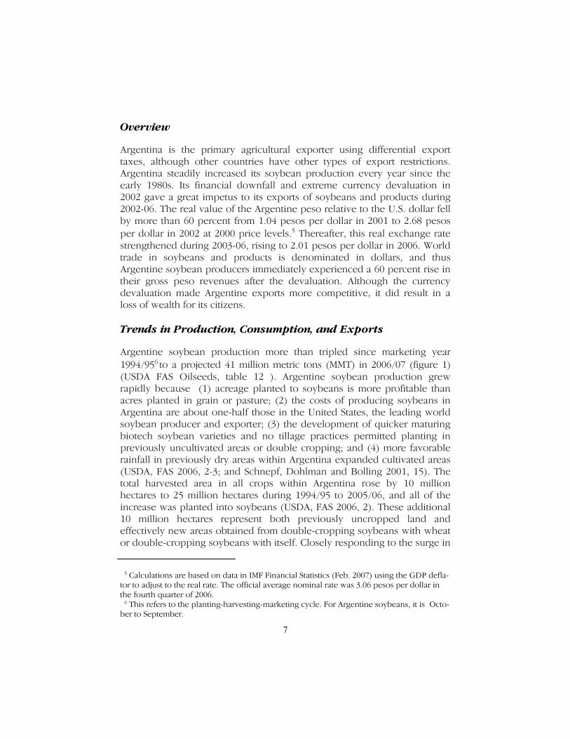
soybean production, Argentine production of soybean oil and meal (nearly 99 percent of which is exported) tripled. Argentina overtook neighboring Brazil and became the world’s leading exporter of soybean oil and meal in marketing year 1996/97. Exports of Argentine soybean oil and meal similarly tripled during this same period. The annual growth rate of Argentine exports of soybean meal and soybean oil generally exceeded that of Argentine soybean production and of exports of soybeans during 1993/94 to 2004/05 as the domestic processing industry consumed a greater share of soybeans (figure 2). As a share of world exports, the Argentine share for soybeans rose only slightly, but its share of soybean oil exports rose from about 35 percent to 50 percent of world exports (figure 3). The annual soybean-processing capacity in Argentina nearly doubled in this period from 17 MMT in 1994 to 32 MMT in 2005 (McKee 2005, 33; and Schnepf, Dohlman, and Bolling, 2001, 25). Plant expansions in 2006 further raised soybean processing capacity to 40 MMT.7 Such expansion involved the construction of the two largest soybean processing plants in

1993/941994/95

1995/961996/97

1997/981998/99

1999/20002000/01

2001/022002/03

2003/042004/05

0

5,000

10,000

15,000

20,000

25,000

30,000

35,000

40,000

Soybean production Soybean exportsSoybean meal exports Soybean oil exports

Figure 1 Soybeans, soybean oil, and soybean meal: Argentine production and exports, 1993/94 to 2004/05.

Source: USDA, FAS, Oilseeds World Markets and Trade, various months.

7 The “big-four” world agricultural exporting companies, ADM, Bunge, Cargill, and Drey-fus, announced a $750 million investment that includes port and terminal infrastructure McKee 2005, 33.

9

1993/941994/95

1995/961996/97

1997/981998/99

1999/20002000/01

2001/022002/03

2003/042004/05

0

100

200

300

Soybean production Soybean exportsSoybean meal exports Soybean oil exports

Figure 2 Soybeans, soybean oil, and soybean meal: Rate of growth in Argentine production and exports, 1993/94 to 2004/05.

Source: USDA, FAS, Oilseeds World Markets and Trade, various months.

1992/931993/94

1994/951995/96

1996/971997/98

1998/991999/2000

2000/012001/02

2002/032003/04

2004/05

0

10

20

30

40

50

Soybeans Soybean meal Soybean oil

Figure 3 Soybeans, soybean oil, and soybean meal: Rate of growth in Argen-tine production and exports, 1992/93 to 2004/05.

Source: USDA, FAS, Oilseeds World Markets and Trade, various months.

10

the world, each with a daily capacity between 15,000 and 18,000 metric tons (McKee 2005, 33)8. History of Argentine Export Tax

Argentina has used export taxes mainly to collect revenue, and to promote exports of processed, higher valued agricultural products, as part of an ISI strategy (Schnepf, Dohlman, and Bolling 16). In the 1980s, agricultural export taxes accounted for nearly one-third of Argentine Federal tax receipts (Meike 6). Argentina in 2005 applied differential export taxes to soybean, sunflower-seed, peanut and cottonseed products. Argentina applied differential tax rates to wheat flour, meat products, and milled rice exports. In 2005, export taxes on Argentine soybeans, soybean oil and soybean meal were respectively 23.5 percent ad valorem equivalent (AVE), 19.3 percent AVE, and 20 percent AVE, according to the USDA (figure 4) (USDA, FAS, Argentina Annual 2005, 8). In 2005 export taxes on oilseeds and products generated $1.4 billion of revenue, most of which went to support domestic social programs unrelated to agriculture (USDA, FAS, 2006, 3). Argentina taxed agricultural exports for many decades; its export tax on soybeans was reduced from 41 AVE percent in May 1989 to 3.5 percent AVE on soybeans (and its tax on soybean oil exports to 1.0 percent) during the 1990s. However, following its economic crisis in the 2002, Argentina raised the soybean tax to its current rate of 23.5 percent, and the tax on soybean oil and meal to 19.3 and 20.0 percent, respectively (figure 4). In 2005/06, the 3.75 percent ad valorem tax differential between soybeans and soybean oil amounted to about $8.50 per metric ton of soybeans (based on an Argentine soybean price of $227 per metric ton in 2005/06; (USDA, FAS, Oilseeds, table 20)). The differential export tax, which amounted to $8.50 per metric ton of soybeans in 2005/06, created an incentive for companies to expand soybean processing in Argentina. One would expect that such an incentive would result in less soybean processing by major soybean-producing countries. Countries, which have imported soybeans for domestic

8 A typical U.S. soybean processing plant has a daily 2,000-ton capacity. The largest U.S. soybean processing plants have daily capacity of 4,000 to 5,000 tons each, according to Milling and Baking News, Sept. 17, 1996, 10, and Oct. 26, 1999, 11; Feedstuffs, Aug. 5, 1996,5.

11

processing, would tend to reduce their imports of soybeans and increase the imports of the two co-products (Fabiosa, Beghin, de Cara, Fang, Isik, and Matthey, 870; and Fabiosa and Beghin 13-15). The variable processing costs of soybeans in Argentina and Brazil in the mid to late 1980s amounted to $14 per metric ton of soybeans processed, as compared to a $20-per-metric-ton cost in the United States (USITC 1987, table 8-7). The tax savings because of the export tax on soybeans amounted in 2005/06 to 43 percent of the variable costs of processing soybeans into soybean oil and soybean meal. A reduction in the price of soybean meal and oil is likely to affect exports of soybean oil and meal because the products are highly interchangeable and price competition is intense.

1993/941994/95

1995/961996/97

1997/981998/99

1999/20002000/01

2001/022002/03

2003/042004/05

-5

0

5

10

15

20

25

Soybeans Soybean oil Soybean meal

Figure 4 Soybeans, soybean oil, and soybean meal: Argentine production and exports, 1993/94 to 2004/05.

Source: Randall Schnepf, Erik Dohlman and Christine Bolling, USDA, ERS, Agriculture in Brazil and Argentina, December 2001, pp. 17-21; USDA, ERS, “Export Taxes Hinder Farm Benefits from Argentina Currency Devaluation,” Oil Crops Situation and Outlook Report, Oct. 2002, pp. 13-16; and USDA, FAS, Argentina Oilseeds and Production

Note: A negative number indicates an export subsidy instead of an export tax. Markets and Trade, various months.

12

Modeling the Argentine Export Tax

Model

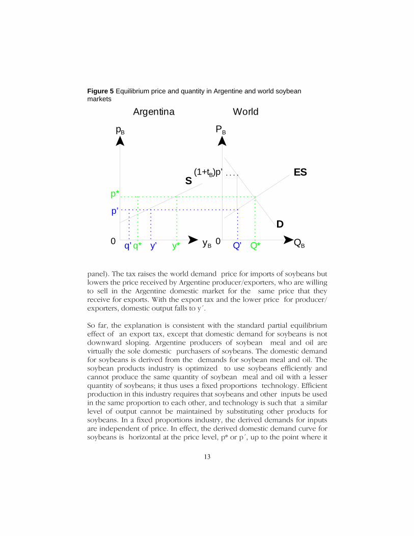
An equilibrium displacement model was used to simulate the effect on the observed equilibrium of changing the export taxes on Argentine soybean products. Storage or other dynamic features are not included. A key characteristic of the model is that soybean oil and meal are jointly produced in fixed proportions from soybeans and other inputs. The model has three products (soybeans, soybean oil and soybean meal) and two regions (Argentina and the rest of the world). In keeping with a common assumption in modeling oilseed products, a homogeneous products or perfect substitutes model was used.9 Such a model assumes that similar products are the same regardless of source. Excess supply (domestic production minus domestic consumption) is equal to the demand for imports from the rest of the world. As previously stated, Argentina is the world’s largest exporter of both soybean oil and soybean meal and is one of the world’s largest exporters of soybeans. Thus, Argentina is assumed to be a large country for these products and has, in each case, an upward sloping excess supply curve. This model assumes that other large producers, such as Brazil and the United States, hold supply constant, and supply from these countries is not modeled. Thus, the effects of any increased exports from these countries into Argentina is ignored. Historically Argentina’s imports of soybeans have been quite low; for example, its soybean imports were only 1.2 percent of domestic production in marketing year 2005/06. The model is mathematically derived in appendix A; a graphical explanation is presented next. Without an export tax, Argentina would produce y* tons of soybeans and consume q* tons domestically (figure 5). In this case, the excess supply of soybeans Q* would equal y* - q*, and the equilibrium price in both the Argentine and world markets would be p*. Currently, however, an ad valorem export tax (tB) is in place that separates the world demand price from the export supply price; Argentine exporters receive a price of p´ per ton, and demanders from the rest of the world pay (1+tB)p´ per ton (right

9 See Piggott and Wohlgenant (2002) or Meilke, Wensley, and Cluff (2001) for examples of homogeneous product soybean models.

13

panel). The tax raises the world demand price for imports of soybeans but lowers the price received by Argentine producer/exporters, who are willing to sell in the Argentine domestic market for the same price that they receive for exports. With the export tax and the lower price for producer/exporters, domestic output falls to y´. So far, the explanation is consistent with the standard partial equilibrium effect of an export tax, except that domestic demand for soybeans is not downward sloping. Argentine producers of soybean meal and oil are virtually the sole domestic purchasers of soybeans. The domestic demand for soybeans is derived from the demands for soybean meal and oil. The soybean products industry is optimized to use soybeans efficiently and cannot produce the same quantity of soybean meal and oil with a lesser quantity of soybeans; it thus uses a fixed proportions technology. Efficient production in this industry requires that soybeans and other inputs be used in the same proportion to each other, and technology is such that a similar level of output cannot be maintained by substituting other products for soybeans. In a fixed proportions industry, the derived demands for inputs are independent of price. In effect, the derived domestic demand curve for soybeans is horizontal at the price level, p* or p´, up to the point where it

Argentina World

QByB

PBpB

ES

D

S(1+tB)p’

p*

p’

Q*Q’y’q’ q* y*0 0

Figure 5 Equilibrium price and quantity in Argentine and world soybean markets

14

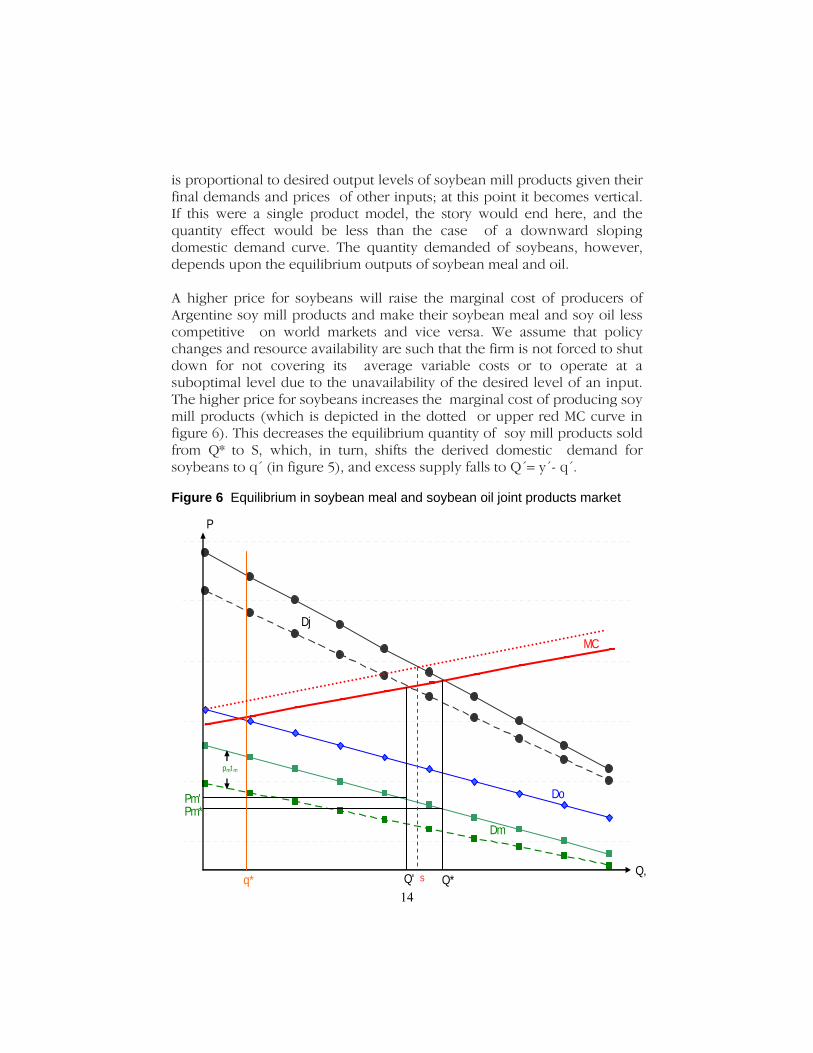
is proportional to desired output levels of soybean mill products given their final demands and prices of other inputs; at this point it becomes vertical. If this were a single product model, the story would end here, and the quantity effect would be less than the case of a downward sloping domestic demand curve. The quantity demanded of soybeans, however, depends upon the equilibrium outputs of soybean meal and oil. A higher price for soybeans will raise the marginal cost of producers of Argentine soy mill products and make their soybean meal and soy oil less competitive on world markets and vice versa. We assume that policy changes and resource availability are such that the firm is not forced to shut down for not covering its average variable costs or to operate at a suboptimal level due to the unavailability of the desired level of an input. The higher price for soybeans increases the marginal cost of producing soy mill products (which is depicted in the dotted or upper red MC curve in figure 6). This decreases the equilibrium quantity of soy mill products sold from Q* to S, which, in turn, shifts the derived domestic demand for soybeans to q´ (in figure 5), and excess supply falls to Q´= y´- q´.

MC

P

Q,

Do

Dm

Q*Q'q*

Pm*Pm'

pmt m

Dj

S

Figure 6 Equilibrium in soybean meal and soybean oil joint products market

15

Incurring the cost of acquiring crushed soybeans enables the production of soybean oil and meal. Soybean oil and meal are jointly produced from crushed soybeans; the oil is expressed, and the remainder is processed as soybean meal. Soybean oil and meal are true joint products of crushed soybeans, and the production of soybean meal does not compete with the production of soybean oil for the same part of crushed soybeans. The condition for equilibrium in competitive output markets for the joint products is that the marginal cost of the joint product equals the sum of the benefits of the production, which is the vertical (price) sum of the demand for the joint products.10 Next, demands for soybean mill products are discussed. The domestic demand for soybean oil, which is used primarily for cooking, is believed to be price inelastic because Argentineans do not typically use soybean oil, as previously discussed. Similarly, the domestic demand for soybean meal, which is often used as a feed supplement for livestock and poultry, is believed to be price-inelastic as Argentineans do not typically feed meal to livestock and have little poultry production. Soybean meal and soybean oil are scaled into units that can be produced with one metric ton of crushed soybeans.11 The fixed or inelastic domestic demand for soybean meal is denoted by q* (figure 6); a similar vertical demand exists for soybean oil, although it is not depicted to avoid overloading the graph. Let Dj denote the vertical sum of the world demand for imports of soybean meal (DM) and soybean oil (DO). Equilibrium is the point where the marginal cost of the joint product (MC) intersects the joint product demand curve (Dj). The equilibrium export quantity of soybean meal is found by subtracting domestic production from this point on the quantity axis (Q*-q*). Market-clearing prices are read off the price axis from the point where the vertical line below the intersection of the MC and demand curves for the joint product crosses the demand curves for the soy mill products (PM* for soybean meal; the price of soybean oil is similarly found but not shown to reduce clutter on the graph). Currently an ad valorem tax of tm on exports of soybean meal separates the world demand price Pm=(1+tm)pm from the export supply price pm. (The situation for an export tax on soybean oil is similar but is not depicted to

10 This is a well established economic principle; see, for example, Layard and Walters 1978, 178-179.

11 For the case of joint products, Friedman showed that scaling products into similar units allowed all supply and demand curves to be shown on the same graph (Friedman 1976, 153-160).

16

avoid confusion on the graph.) The green hashed line (Dm) shows the export demand for soybean meal at supply prices when the tax is imposed on exports of soybean meal.12 To find the equilibrium quantity with this tax in place, we add the demand for soybean meal at the export supply price to the demand for soybean oil (Do) to construct the effective demand curve for the joint product (hashed Dj) and find its intersection with the curve for the marginal cost of the joint product. The resulting equilibrium quantity is Q´, and the world demand prices are found as before (Pm´ in the case of soybean meal). We see that the tax on exports of soybean meal reduces the export quantities of both soybean meal and soybean oil; in the case of soybean meal, the reduction is from Q*-q* to Q´-q*. The world demand price for both soybean meal and oil increases, while the price received by Argentine exporters decreases. It is interesting to note that an export tax on one of two or more joint products shifts the equilibrium quantities and demand prices by smaller amounts than in the case of a similar export tax on a single nonjoint product because equilibrium is determined by the intersection of the joint demand curve (one of whose components would not change) with the marginal cost of the joint product. The story is similar when an export tax is also imposed on soybean oil; the effective joint demand at the supply price would be the sum of the demands at the supply prices. Also, one can see that some large export tax on one of the two joint products would have the same effect on quantities and prices as two smaller export taxes on each of the joint products. Generally, the export taxes decrease equilibrium quantities, raise the world prices paid by foreign buyers, and lower the prices received by exporters.

Data

Argentine production, exports and prices for soybeans, soybean oil, and soybean meal for crop year 2004/05 are shown in table 1. As previously reported, Argentina applied differential export taxes on soybeans, soybean oil, and soybean meal of, respectively, 23.5 percent, 19.3 percent, and 20.0 percent in 2005. Argentine consumption of soybean oil and meal is minimal; about 9 per-cent of domestic oil production and less than 1 percent of domestic meal

12 Note that the difference between the effective demand price and effective supply price is (1+tM)pM-pM=t MpM.

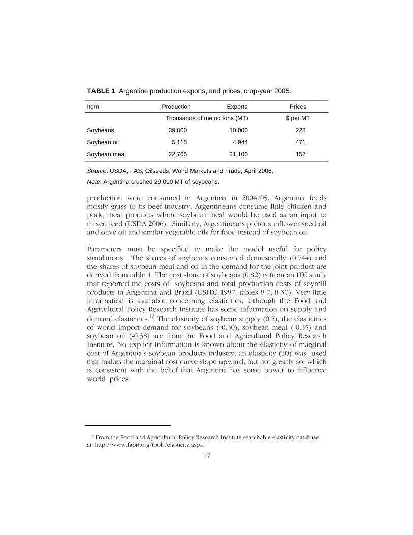
17

production were consumed in Argentina in 2004/05. Argentina feeds mostly grass to its beef industry. Argentineans consume little chicken and pork, meat products where soybean meal would be used as an input to mixed feed (USDA 2006). Similarly, Argentineans prefer sunflower seed oil and olive oil and similar vegetable oils for food instead of soybean oil. Parameters must be specified to make the model useful for policy simulations. The shares of soybeans consumed domestically (0.744) and the shares of soybean meal and oil in the demand for the joint product are derived from table 1. The cost share of soybeans (0.82) is from an ITC study that reported the costs of soybeans and total production costs of soymill products in Argentina and Brazil (USITC 1987, tables 8-7, 8-30). Very little information is available concerning elasticities, although the Food and Agricultural Policy Research Institute has some information on supply and demand elasticities.13 The elasticity of soybean supply (0.2), the elasticities of world import demand for soybeans (-0.30), soybean meal (-0.35) and soybean oil (-0.38) are from the Food and Agricultural Policy Research Institute. No explicit information is known about the elasticity of marginal cost of Argentina’s soybean products industry, an elasticity (20) was used that makes the marginal cost curve slope upward, but not greatly so, which is consistent with the belief that Argentina has some power to influence world prices.

TABLE 1 Argentine production exports, and prices, crop-year 2005.

Item Production Exports Prices

$ per MT

Soybeans 39,000 10,000 228

Soybean oil 5,115 4,944 471

Soybean meal 22,765 21,100 157

Source: USDA, FAS, Oilseeds: World Markets and Trade, April 2006.

Note: Argentina crushed 29,000 MT of soybeans.

Thousands of metric tons (MT)

13 From the Food and Agricultural Policy Research Institute searchable elasticity database at http://www.fapri.org/tools/elasticity.aspx.

18

Results

This section reports the results from four policy experiments using the model and parameters presented in the previous section. First, only the export tax on soybeans is removed; second, the export taxes on soybean products are removed while leaving the export tax on soybeans in place; third, all export taxes are set to 10 percent, and finally all export taxes are removed. The 23.5 percent export tax on soybeans was totally removed. The largest effects were a decrease in the world price paid by foreign importers and an increase in the export quantity; the price change was dominant due to the inelastic demand (table 2). The domestic exporters’ price of soybeans rose slightly, providing an incentive to increase production. Domestic producers/exporters were willing to sell in the domestic market at the same price that they received in the export market. The higher domestic price for soybeans increased the marginal cost of the joint product, which raised the prices of soybean oil and soybean meal. There was a corresponding relatively small decrease in the outputs of soybean meal and oil. The taxes of 19.3 percent and 20 percent, respectively, on exports of soybean oil and soybean meal were removed, while leaving in place the export tax on soybeans. Elimination of these export tax wedges decreased world prices of soybean oil and soybean meal for foreign importers and increased the domestic exporters’ prices while the quantity of these exports expanded (table 3). The effective increases in demands for these products raised the domestic derived demand for soybeans, which resulted in decreased exports of soybeans. The world and domestic prices of soybeans increased, which was an incentive to boost production; this resulted in a relatively smaller fall in the export quantity of soybeans in comparison with the gain in domestic consumption. TABLE 2 Results from removing the 23.5 percentage export tax on soybeans (percentage change).

World import price

Export quantity Domestic or exporters’ price

Soybeans -18.0 5.4 1.2

Soybean oil 1.0 -0.4 1.0

Soybean meal 1.0 -0.4 1.0

Source: Calculations from model.

Domestic consumption

-0.4

unchanged

unchanged

19

Next, export taxes on soybeans, soybean oil, and soybean meal were all set at 10 percent (by lowering the export taxes on soybeans, soybean oil, and soybean meal, respectively, by 13.5 percent, 9.3 percent, and 10 percent). In each case, decreasing the tax wedges lowered world prices for foreign importers, raised domestic or exporters’ prices, and export quantities expanded (table 4). The effective increases in demands for soybean meal and soybean oil shifted the derived domestic demand for soybeans at the same time that the effective demand for soybeans was increasing in the world market, which raised the producer/exporter price of soybeans and provided an incentive to boost domestic production of soybeans. The higher domestic price of soybeans also increased the marginal cost of the joint product. As both marginal cost and demand for the joint product shifted upward, price changed relatively more than quantity. Joint products could be a reason for maintaining differential export taxes and taxing the co-products proportionally less than other products, but in this case we see roughly similar responses by all products.

TABLE 3 Results from removing export taxes of 19.3 percent and 20 percent, respectively on soybean oil and soybean meal (percentage change).

World import price

Export quantity Domestic or exporters’ price

Soybeans 3.3 -1.0 3.3

Soybean oil -12.7 4.8 3.5

Soybean meal -13.7 4.8 2.9

Source: Calculations from model.

Domestic consumption

4.8

unchanged

unchanged

TABLE 4 Results from setting export taxes on soybeans, soybean oil, and soybean meal at 10 percent for each product (from 23.5, 19.3 percent, and 20 percent, respectively), (percentage change).

World import price

Export quantity Domestic or exporters’ price

Soybeans -8.7 2.6 2.3

Soybean oil -5.7 2.2 2.1

Soybean meal -6.2 2.2 2.1

Source: Calculations from model.

Domestic consumption

2.2

unchanged

unchanged

20

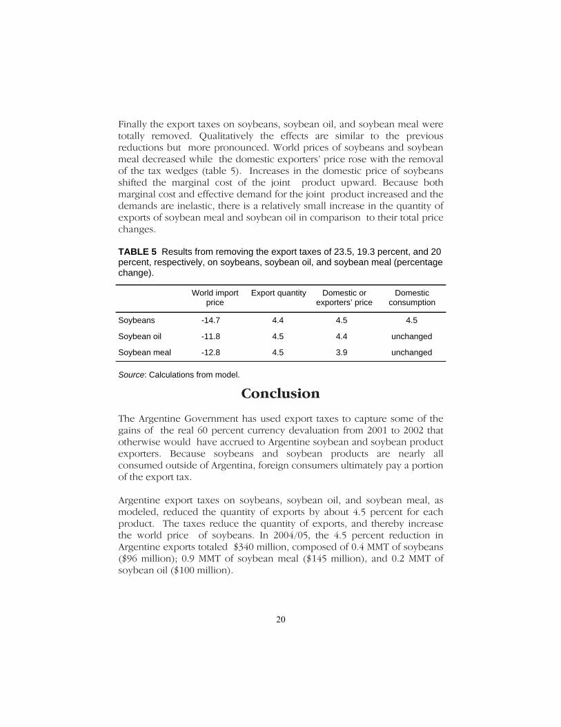
Finally the export taxes on soybeans, soybean oil, and soybean meal were totally removed. Qualitatively the effects are similar to the previous reductions but more pronounced. World prices of soybeans and soybean meal decreased while the domestic exporters’ price rose with the removal of the tax wedges (table 5). Increases in the domestic price of soybeans shifted the marginal cost of the joint product upward. Because both marginal cost and effective demand for the joint product increased and the demands are inelastic, there is a relatively small increase in the quantity of exports of soybean meal and soybean oil in comparison to their total price changes.

Conclusion

The Argentine Government has used export taxes to capture some of the gains of the real 60 percent currency devaluation from 2001 to 2002 that otherwise would have accrued to Argentine soybean and soybean product exporters. Because soybeans and soybean products are nearly all consumed outside of Argentina, foreign consumers ultimately pay a portion of the export tax. Argentine export taxes on soybeans, soybean oil, and soybean meal, as modeled, reduced the quantity of exports by about 4.5 percent for each product. The taxes reduce the quantity of exports, and thereby increase the world price of soybeans. In 2004/05, the 4.5 percent reduction in Argentine exports totaled $340 million, composed of 0.4 MMT of soybeans ($96 million); 0.9 MMT of soybean meal ($145 million), and 0.2 MMT of soybean oil ($100 million).

TABLE 5 Results from removing the export taxes of 23.5, 19.3 percent, and 20 percent, respectively, on soybeans, soybean oil, and soybean meal (percentage change).

World import price

Export quantity Domestic or exporters’ price

Soybeans -14.7 4.4 4.5

Soybean oil -11.8 4.5 4.4

Soybean meal -12.8 4.5 3.9

Source: Calculations from model.

Domestic consumption

4.5

unchanged

unchanged

21

If Argentina eliminated its 23.5 percent tax on soybean exports, but retained export taxes of 19.3 and 20 percent, respectively, on soybean oil and meal exports, Argentine soybean exports would rise by 5 percent, but its exports of oil and meal would remain largely unchanged (dropping about 1 percent). If Argentina applied a lower, uniform tax rate of 10 percent on all three soybean products, exports of all three products each rise by about 2 percent. The peso devaluation of 60 percent in real terms likely had a greater effect on Argentine soy exports than export taxes. Because revenues are priced in dollars but many inputs are priced in Argentine pesos, exports would increase as effective excess supply shifts outward. Because soybeans are also exported, producers of soy mill products, however, would have to pay the equivalent of the world dollar price for soybeans, adjusted for taxes, because soybean producers have the alternative of selling directly into the world market. Still, producers of soy mill products would benefit as part of their costs are denominated in pesos.14 Using the results of another study (Andino, Mulik, and Koo 2005, 13),15 the 60 percent devaluation would be expected, ceteris paribus, to increase Argentine exports of soybeans and soybean products by about 30 percent. In the four years after the devaluation (marketing years 2001/02 to 2005/06), the combined exports of Argentine soy products rose by 53 percent on a soybean-oil equivalent basis and 38 percent on a soybean-meal equivalent basis.16

14 Although this study has not directly dealt with transport costs, local soy mill producers would face lower transport margins when purchasing soybeans locally.

15 The estimated elasticity of soybean exports to devaluations in Argentina and Brazilian currency is at 0.50.

16 This assumes an oil yield of 18 percent, and a meal yield of 80 percent from soybeans, and then adding together separately the oil and meal equivalents. Data from FAS, USDA. This assumes an oil yield of 18 percent, and a meal yield of 80 percent from soybeans, and then adding together separately the oil and meal equivalents. Data from FAS, USDA.

22

References

Ash, Mark, and Erik Dohlman. 2000-2002. Oil Crops Situation and Outlook Report. Washington DC: U.S. Department of Agriculture, Economic Research Service. October. http://www.ers.usda.gov/Publications/Outlook.

Andino, Jose, Kranti Mulik, and Won Koo. 2005. The impact of Brazil and

Argentina’s currency devaluation on U.S. soybean trade. Center for Agricultural Policy and Trade Studies, Department of Agribusiness and Applied Economics, North Dakota State University, Fargo, ND.

American Oilseed Coalition. 2002. Comments regarding the Doha multilateral

trade negotiations and agenda in the WTO Trade Policy Staff Committee, Office of the United States Trade Representative.

Bidard, Christian, and Guido Erreygers. 1998. Sraffa and Leontief on joint

production. Review of Political Economy 10:427-446. Childs, Nathan, and Linwood Hoffman. 1999. Upcoming WTO negotiations:

Issues for the U.S. rice sector. Rice Situation and Outlook Report. Washington DC: USDA, ERS. http://www.ers.usda.gov/Publications/Outlook/

Fabiosa, Jay, John Beghin, Stephane de Cara, Cheng Fang, Murat Isik, and Holger

Matthey. 2003. Agricultural markets liberalization and the Doha Round. Proceedings of the 25th International Conference of Agricultural Economics. August.

Fabiosa, Jay, and John Beghin. 2002. The Doha Round of the WTO: Appraising

further liberalization of agricultural markets. FAPRI Working Paper 02-WP 317, Iowa State University, November. www.fapri.org

Feedstuffs. 1996. Feenstra, Robert C. 1986. Trade policy with several goods and ‘market linkages.’

Journal of International Economics 20:249-267. Food and Agricultural Policy Research Institute (FAPRI). 2007. Elasticity database.

http://www.fapri.org/tools/elasticity.aspx Friedman, Milton. 1976. Price Theory. Chicago: Aldine Publishing Co.

23

Hoffman, Linwood Erik Dohlman, and Mark Ash. 1999. Upcoming WTO negotiations: Issues for the U.S. oilseed sector, Oil crops situation and outlook yearbook, ERS, USDA, October 1999. http://www.ers.usda.gov/Publications/Outlook/

Kazeki, Jan. Export Duties. 2006. OECD Trade Policy Studies Looking Beyond

Tariffs The Role of Non-Tariff Barriers in World Trade 2006, no. 1, OECD. http://www.oecd.org

Lamy, Pascal (Director-General of the WTO). 2007. Report to the WTO General

Council. February 7. Layard, P.R.G., and A.A. Walters. (1978). Microeconomic theory. 178-179. Manes, R.P., and Vernon L. Smith. 1965. Economic joint cost theory and

accounting practice. Accounting Review 40:31-35. McKee, David. 2005. South America: The world’s soybean super supplier. World

Grain. http://www.world-grain.com Meilke, Karl, Mitch Wensley, and Merritt Cluff. 2001. The impact of trade

liberalization on the international oilseed complex. Review of International Agricultural Economics 23:2-17.

Mielke, Myles. 1984-1996. Argentine Agricultural Policies in the Grain and Oilseed

Sectors. FAER Report No. 206, USDA, ERS. Milling and Baking News. 1996-1999. http://www.bakingbusiness.com/

Organization for Economic Cooperation and Development (OECD). 2003.

Analysis of non-tariff measures: The case of export duties. Working Party of the Trade Committee, TD/TC/WP(2002)54/Final. January 31. www.oecd.org

Piermartini, Roberta. 2004. The role of export taxes in the field of primary

commodities. Geneva, Switzerland: ERSD, WTO. September 8. http://www.wto.org

Piggott, Nicholas E., and Michael K. Wohlgenant. 2002. Price elasticities, joint

products, and international trade. Australian Journal of Agricultural and Resource Economics 46:87-500.

Roller, Lars-Hendrik. 1990. Proper quadratic cost functions with an application to

the Bell System. Review of Economics and Statistics 72:2.

24

Schnepf, Randall, Erik Dohlman, and Christine Bolling. 2001. Agriculture in Brazil and Argentina. ERS Agriculture and Trade Reports No. WRS013, ERS, USDA. http://www.ers.usda.gov/Publications/WRS013/

Tarp-Jensen, Henning, Sherman Robinson, and Finn Tarp. 2002. General

Equilibrium Measures of Agricultural Policy Bias in Fifteen Developing Countries. International Food Policy Research Institute

Toulan, Omar N. 2002. Measuring the impact of market liberalization on export

behavior: The case of Argentina. International Trade Journal 16:105-128. U.S. Department of Agriculture. ERS. 2002. Agricultural Exchange Rate Data Set.

http://www.ers.usda.gov/Data/ExchangeRates/retrieved. USDA. 2005. Foreign Agriculture Service (FAS). Argentina Oilseeds and Products

Annual, 2005. GAIN Report No. AR5017, May 19, 2005. http://www.fas.usda.gov/scriptsw/attacherep/default.asp

25

Appendix

The model used to estimate the effects of altering the export taxes on Argentine soybean products is derived in this appendix. The following constant elasticity specification represents Argentine output or supply of soybeans (yB). Equation 1 where pB

is the domestic price received by producers (who may also be exporters), k is a parameter based on initial conditions, and ε is the supply elasticity. Let qB denote the domestic demand for soybeans, and let QB denote the world demand for imports of soybeans, which is a function of the world price. When an export tax is in place, the world price or foreign demand price PB is separated from the domestic price by the ad valorem export tax tB; thus PB=(1+tB) pB. Argentine excess supply of soybeans is set equal to the world demand for imports of soybeans, which is also specified as a constant elasticity relationship, as shown below where the expression for the domestic price is substituted for the world price on the right hand side. Equation 2

yB − qB = QB(PB) = KB[(1+ tB) pB]η where η is the elasticity of demand for foreign imports of soybeans and KB is a parameter related to initial conditions. Because soybean oil and meal are produced in fixed proportions from crushed soybeans and other factors of production, such as labor and capital, a fixed proportions or Leontief production function for the separate outputs of soybean meal ym and soybean oil yO might be specified.17 It is,

17 Strictly speaking the Leontief production function is not consistent with joint production. See discussion in Christian Bidard and Guido Erreygers. The relevant economic entity is clearly the joint product; see R.P. Manes and Vernon L. Smith, and Roman Weil. Output lev-els implied by optimizing a joint product profit function generally differ from those ob-tained by optimizing profit functions for the individual products.

y p k pB B B( ) = ε

26

however, more convenient to define the joint product w as the sum of the outputs of soybean oil and soybean meal (w=yM+yO, where yM and yO are scaled as output produced per metric ton of soybeans). The fixed proportions production function for the joint product is-

where z is a component representing other inputs including capital, labor, entrepreneurial expertise, etc., and the αs are positive input-output coefficients. The most efficient input utilization occurs when w = α qB = αZ z; no input can be decreased at this point without lowering output, and all inputs must increase to raise output. The cost-minimizing or conditional input demand for soybeans in the joint production of soybean meal and soybean oil is thus qB=w/α, which is independent of price.18 Substituting this conditional input demand and equation 1 into equation 2 results in equation 3. Equation 3

The price of soybeans in the domestic market indirectly affects the location of its own demand curve because the marginal cost of the joint product (discussed below) is a function of the soybean price. The associated cost function has the following simple form in which output appears as a function:19

w = min (α q B , αZ z )

[ ]kp w K t pB B B Bε η

α= + +( )1

18 In a model not using the fixed proportions technology, Piggott and Wohlgenant, building on earlier work by Houck, show that the derived price elasticity of domestic demand for soybeans is a harmonic weighted average of the total demand (both domestic and foreign) elasticities for soybean meal and soybean oil. While that relationship does not hold in this model, the derived domestic demand for soybeans shifts with changes in the prices of soy-bean meal and soybean oil; in effect, domestic demand for soybeans is determined in the output markets for soybean meal and soybean oil.

19 This small generalization of the Leontief cost function differs from the generalized Leon-tief functional form which econometricians have long used to permit substitution among inputs. The use here is more in line with Lars-Hendrik Roller. Specifically it permits marginal cost, the relevant supply concept, to slope upward, which is in line with the large country assumption.

27

Equation 4

where pZ is the composite costs of inputs other than crushed soybeans, and f is a continuous function of w with a positive first derivative (f ‘> 0). The domestic demands for soybean meal and soybean oil are believed to be price-inelastic, as discussed, and are denoted by qM* and qO*, respectively. The rest of the world’s demands for imports of soybean meal and oil have constant elasticity specifications similar to the demand for imports of soybeans. These equations are inverted to place them in price terms. The inverse demand for soybean meal, pM, is shown below. Equation 5

where pM is the domestic exporters’ price, QM is the quantity demanded, tM is the export tax, μ is the own-price demand elasticity and KM is a parameter dependent on initial conditions. There is a similar equation for soybean oil with λ as its own-price elasticity and t0 as the ad valorem tax on exports or soybean oil. Then, setting the export supply of the joint product equal to the demands or equivalently setting marginal cost of the joint product equal to the sum of its uses leads to the following equation. Equation 6

where the right-hand side p’s are the inverse demands and the q’s are the inelastic domestic demands.

c p p wp p

f wB ZB Z

Z

( , , ) ( )= +⎛⎝⎜

⎞⎠⎟

α α

p QK tM

M

M M

=⎛⎝⎜

⎞⎠⎟

+

1

11

μ

p pf w q q p Q t p Q tB Z

ZM O M M M O O Oα α

+⎛⎝⎜

⎞⎠⎟ ′ = + + +( ) ( , ) ( , )* *

28

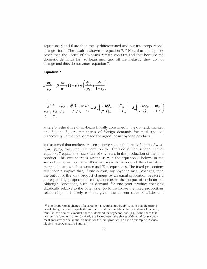
Equations 3 and 6 are then totally differentiated and put into proportional change form. The result is shown in equation 7.20 Note that input prices other than the price of soybeans remain constant and that because the domestic demands for soybean meal and oil are inelastic, they do not change and thus do not enter equation 7. Equation 7

where β is the share of soybeans initially consumed in the domestic market, and δM and δO are the shares of foreign demands for meal and oil, respectively, in the total demand for Argentinean soybean products. It is assumed that markets are competitive so that the price of a unit of w is pB/α + pZ/αZ; thus, the first term on the left side of the second line of equation 7 equals the cost share of soybeans in the production of the joint product. This cost share is written as γ in the equation 8 below. In the second term, we note that df’(w)w/f’(w) is the inverse of the elasticity of marginal costs, which is written as 1/E in equation 8. The fixed proportions relationship implies that, if one output, say soybean meal, changes, then the output of the joint product changes by an equal proportion because a corresponding proportional change occurs in the output of soybean oil. Although conditions, such as demand for one joint product changing drastically relative to the other one, could invalidate the fixed proportions relationship, it is likely to hold given the current state of affairs and

20 The proportional change of a variable x is represented by dx/x. Note that the propor-tional change of a sum equals the sum of its addends weighted by their share of the sum; thus β is the domestic market share of demand for soybeans, and (1-β) is the share that goes to the foreign market. Similarly the δ’s represent the shares of demand for soybean meal and soybean oil in the demand for the joint product. This is an example of “Jones algebra” (see Feenstra, 14 and 17).

( )ε β β η

α

α α

δμ

δλ

dpp

dww

dpp

dtt

p

p pdpp

df w wf w

dww

dQQ

dtt

dQQ

dtt

B

B

B

B

B

B

B

B Z

Z

B

BM

M

M

M

MO

O

O

O

O

= + − ++

⎛⎝⎜

⎞⎠⎟

++ = −

+⎛⎝⎜

⎞⎠⎟ + −

+⎛⎝⎜

⎞⎠⎟

11

11

11

1'( )'( )

29

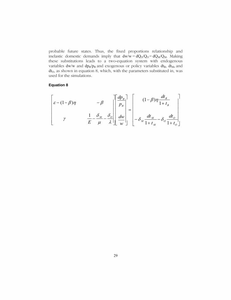
probable future states. Thus, the fixed proportions relationship and inelastic domestic demands imply that dw/w = dQO/QO = dQM/QM. Making these substitutions leads to a two-equation system with endogenous variables dw/w and dpB/pB and exogenous or policy variables dtB, dtM, and dtO, as shown in equation 8, which, with the parameters substituted in, was used for the simulations. Equation 8

ε β η β

γδμ

δλ

β η

δ δ

− − −

− −

⎡

⎣

⎢⎢⎢⎢⎢

⎤

⎦

⎥⎥⎥⎥⎥

⎡

⎣

⎢⎢⎢⎢⎢

⎤

⎦

⎥⎥⎥⎥⎥

=

−+

−+

−+

⎡

⎣

⎢⎢⎢⎢⎢

⎤

⎦

⎥⎥⎥⎥⎥

( ) ( )1

1

11

1 1E

dpp

dww

dtt

dtt

dtt

M O

B

B

B

B

MM

MO

O

O