Exponential utility indifference valuation in a general ...mschweiz/Files/CFMS2009.pdf ·...
38
Exponential utility indifference valuation in a general semimartingale model Christoph Frei and Martin Schweizer This version: 25.02.2009. (In: Delbaen, F., R´ asonyi, M. and Stricker, C. (eds.), “Optimality and Risk — Modern Trends in Mathematical Finance. The Kabanov Festschrift”, Springer, Berlin (2009), 49–86) This paper is dedicated to Yuri Kabanov on the occasion of his 60th birthday. We hope he likes it even if it is not short . . . Abstract We study the exponential utility indifference valuation of a contingent claim H when asset prices are given by a general semimartingale S. Under mild assumptions on H and S, we prove that a no-arbitrage type condition is fulfilled if and only if H has a certain representation. In this case, the indifference value can be written in terms of processes from that representation, which is useful in two ways. Firstly, it yields an interpolation expression for the indifference value which gener- alizes the explicit formulas known for Brownian models. Secondly, we show that the indifference value process is the first component of the unique solution (in a suitable class of processes) of a backward stochastic differential equation. Under additional assumptions, the other components of this solution are BMO-martingales for the minimal entropy martingale measure. This generalizes recent results by Becherer [2] and Mania and Schweizer [19]. Key words: exponential utility, indifference valuation, minimal entropy martingale measure, BSDE, BMO-martingales, fundamental entropy representation (FER) MSC 2000 subject classification: 91B28, 60G48 JEL classification numbers: G13, C60 1 Introduction One general approach to the problem of valuing contingent claims in incomplete markets is utility indifference valuation. Its basic idea is that the investor valuing a Christoph Frei ETH Zurich, Department of Mathematics, 8092 Zurich, Switzerland, e-mail: [email protected] Martin Schweizer ETH Zurich, Department of Mathematics, 8092 Zurich, Switzerland, e-mail: [email protected] 1
Transcript of Exponential utility indifference valuation in a general ...mschweiz/Files/CFMS2009.pdf ·...

Exponential utility indifference valuationin a general semimartingale model
Christoph Frei and Martin SchweizerThis version: 25.02.2009.(In: Delbaen, F., Rasonyi, M. and Stricker, C. (eds.), “Optimality andRisk — Modern Trends in Mathematical Finance. The Kabanov Festschrift”,Springer, Berlin (2009), 49–86)
This paper is dedicated to Yuri Kabanov on the occasion of his 60th birthday. Wehope he likes it even if it is not short . . .
Abstract We study the exponential utility indifference valuation of a contingentclaim H when asset prices are given by a general semimartingale S. Under mildassumptions on H and S, we prove that a no-arbitrage type condition is fulfilled ifand only if H has a certain representation. In this case, the indifference value can bewritten in terms of processes from that representation, which is useful in two ways.Firstly, it yields an interpolation expression for the indifference value which gener-alizes the explicit formulas known for Brownian models. Secondly, we show that theindifference value process is the first component of the unique solution (in a suitableclass of processes) of a backward stochastic differential equation. Under additionalassumptions, the other components of this solution are BMO-martingales for theminimal entropy martingale measure. This generalizes recent results by Becherer [2]and Mania and Schweizer [19].
Key words: exponential utility, indifference valuation, minimal entropy martingalemeasure, BSDE, BMO-martingales, fundamental entropy representation (FER)MSC 2000 subject classification: 91B28, 60G48JEL classification numbers: G13, C60
1 Introduction
One general approach to the problem of valuing contingent claims in incompletemarkets is utility indifference valuation. Its basic idea is that the investor valuing a
Christoph FreiETH Zurich, Department of Mathematics, 8092 Zurich, Switzerland,e-mail: [email protected]
Martin SchweizerETH Zurich, Department of Mathematics, 8092 Zurich, Switzerland,e-mail: [email protected]
1

2 Christoph Frei and Martin Schweizer
contingent claim H should achieve the same expected utility in the two cases where(1) he does not have H, or (2) he owns H but has his initial capital reduced by theamount of the indifference value of H. Exponential utility indifference valuationmeans that the utility function one uses is exponential.
Even in a concrete model, it is difficult to obtain a closed-form formula for the in-difference value. The majority of existing explicit results are for Brownian settings;see for instance Frei and Schweizer [10] and the references therein. In more generalsituations, Becherer [2] and Mania and Schweizer [19] derive a backward stochasticdifferential equation (BSDE) for the indifference value process. While [19] assumesa continuous filtration, the framework in [2] has a continuous price process drivenby Brownian motions and a filtration generated by these and a random measureallowing the modeling of non-predictable events.
The main contribution of this paper is to extend the above results to a settingwhere asset prices are given by a general semimartingale. We show that the ex-ponential utility indifference value can still be written in a closed-form expressionsimilar to that known for Brownian models, although the structure of this formula ishere much less explicit. Independently from that, we establish a BSDE formulationfor the dynamic indifference value process. Both of these results are based on a rep-resentation of the claim H and on the relationship between a notion of no-arbitrage,the form of the so-called minimal entropy martingale measure, and the indifferencevalue.
As our starting point, we take the work of Biagini and Frittelli [3, 4]. Their resultsyield a representation of the minimal entropy martingale measure which we can useto derive a decomposition of a fixed payoff H in a similar way as in Becherer [1]. Wecall this decomposition, which is closely related to the minimal entropy martingalemeasure, the fundamental entropy representation of H
(FER(H)
). It is central to all
our results here, because we can express the indifference value for H as a differenceof terms from FER(H) and FER(0). We derive from this a fairly explicit formula forthe indifference value by an interpolation argument, and we also establish a BSDErepresentation for the indifference value process. Its proof is based on the idea thatthe two representations FER(H) and FER(0) can be merged to yield a single BSDE.This direct procedure allows us to work with a general semimartingale, whereasBecherer [2] as well as Mania and Schweizer [19] use more specific models becausethey first prove some results for more general classes of BSDEs and then applythese to derive the particular BSDE for the indifference value. The price to payfor working in our general setting is that we must restrict the class of solutions ofthe BSDE to get uniqueness. Under additional assumptions, the components of thesolution to the BSDE for the indifference value are again BMO-martingales for theminimal entropy martingale measure; this applies in particular to the value processof the indifference hedging strategy.
The paper is organized as follows. Section 2 lays out the model, motivates, and in-troduces the important notion of FER(H). In Section 3, we prove that the existenceof FER(H) is essentially equivalent to an absence-of-arbitrage condition. Moreover,we develop a uniqueness result for FER(H) and its relationship to the minimal en-tropy martingale measure. Section 4 establishes the link between the exponential

General exponential utility indifference valuation 3
indifference value of H and the two decompositions FER(H) and FER(0). By aninterpolation argument, we derive a fairly explicit formula for the indifference value.In Section 5, we extend to a general filtration the BSDE representation of the indif-ference value by Becherer [2] and Mania and Schweizer [19]. We further provideconditions under which the components of the solution to the BSDE are BMO-martingales for the minimal entropy martingale measure. Section 6 rounds off withan application to a Brownian setting.
2 Motivation and definition of FER(H)
We start with a probability space (Ω ,F ,P), a finite time interval [0,T ] for a fixedT > 0 and a filtration F = (Ft)0≤t≤T satisfying the usual conditions of right-conti-nuity and completeness. For simplicity, we assume that F0 is trivial and FT = F .For a positive process Z, we use the abbreviation Zt,s := Zs/Zt , 0≤ t ≤ s≤ T .
In our financial market, there are d risky assets whose price process S = (St)0≤t≤Tis an Rd-valued semimartingale. In addition, there is a riskless asset, chosen as nu-meraire, whose price is constant at 1. Our investor’s risk preferences are given by anexponential utility function U(x) =−exp(−γx), x∈R, for a fixed γ > 0. We alwaysconsider a fixed contingent claim H which is a real-valued F -measurable randomvariable satisfying EP
[exp(γH)
]< ∞. Expressions depending on H are introduced
with an index H so we can later use them also in the absence of the claim by set-ting H = 0. However, the dependence on γ is not explicitly mentioned. We defineby dPH
dP := exp(γH)/
EP[exp(γH)
]a probability measure PH on (Ω ,F ) equivalent
to P. Note that P0 = P. We denote by L(S) the set of all Rd-valued predictableS-integrable processes, so that
∫ϑ dS is a well-defined semimartingale for each ϑ
in L(S).We always impose without further mention the following standing assumption,
introduced by Biagini and Frittelli [3, 4] for H = 0. We assume that
WH 6= /0 and W0 6= /0, (1)
where WH is the set of loss variables W which satisfy the following two conditions:
1) W ≥ 1 P-a.s., and for every i = 1, . . . ,d, there exists some β i ∈ L(Si) such thatP[∃ t ∈ [0,T ] s.t. β i
t = 0]= 0 and
∣∣∫ t0 β i
s dSis∣∣≤W for all t ∈ [0,T ];
2) EPH
[exp(cW )
]< ∞ for all c > 0.
Clearly, WH = W0 if H is bounded. Lemma 1 at the beginning of Section 3 gives aless restrictive condition on H for WH = W0. The standing assumption (1) is auto-matically fulfilled if S is locally bounded since then 1 ∈WH ∩W0 by Proposition 1of Biagini and Frittelli [3], using PH ≈ P. But (1) is for example also satisfied if His bounded and S = S1 is a scalar compound Poisson process with Gaussian jumps.This follows from Section 3.2 in Biagini and Frittelli [3]. So the model with condi-tion (1) is a genuine generalization of the case of a locally bounded S.
4 Christoph Frei and Martin Schweizer
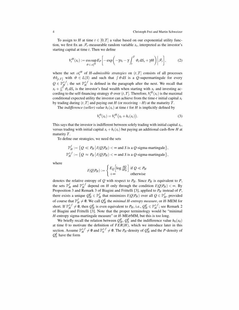
To assign to H at time t ∈ [0,T ] a value based on our exponential utility func-tion, we first fix an Ft -measurable random variable xt , interpreted as the investor’sstarting capital at time t. Then we define
V Ht (xt) := esssup
ϑ ∈A Ht
EP
[−exp
(−γxt − γ
∫ T
tϑs dSs + γH
)∣∣∣∣Ft
], (2)
where the set A Ht of H-admissible strategies on (t,T ] consists of all processes
ϑ I]]t,T ]] with ϑ ∈ L(S) and such that∫
ϑ dS is a Q-supermartingale for everyQ ∈ Pe, f
H ; the set Pe, fH is defined in the paragraph after the next. We recall that
xt +∫ T
t ϑs dSs is the investor’s final wealth when starting with xt and investing ac-cording to the self-financing strategy ϑ over (t,T ]. Therefore, V H
t (xt) is the maximalconditional expected utility the investor can achieve from the time-t initial capital xtby trading during (t,T ] and paying out H (or receiving −H) at the maturity T .
The indifference (seller) value ht(xt) at time t for H is implicitly defined by
V 0t (xt) = V H
t(xt +ht(xt)
). (3)
This says that the investor is indifferent between solely trading with initial capital xt ,versus trading with initial capital xt +ht(xt) but paying an additional cash-flow H atmaturity T .
To define our strategies, we need the sets
P fH :=
Q PH
∣∣ I(Q|PH) < ∞ and S is a Q-sigma-martingale,
Pe, fH :=
Q ≈ PH
∣∣ I(Q|PH) < ∞ and S is a Q-sigma-martingale,
where
I(Q|PH) :=
EQ
[log dQ
dPH
]if Q PH
+∞ otherwise
denotes the relative entropy of Q with respect to PH . Since PH is equivalent to P,the sets P f
H and Pe, fH depend on H only through the condition I(Q|PH) < ∞. By
Proposition 3 and Remark 3 of Biagini and Frittelli [3], applied to PH instead of P,there exists a unique QE
H ∈ P fH that minimizes I(Q|PH) over all Q ∈ P f
H , providedof course that P f
H 6= /0. We call QEH the minimal H-entropy measure, or H-MEM for
short. If Pe, fH 6= /0, then QE
H is even equivalent to PH , i.e., QEH ∈ Pe, f
H ; see Remark 2of Biagini and Frittelli [3]. Note that the proper terminology would be “minimalH-entropy sigma-martingale measure” or H-MEσMM, but this is too long.
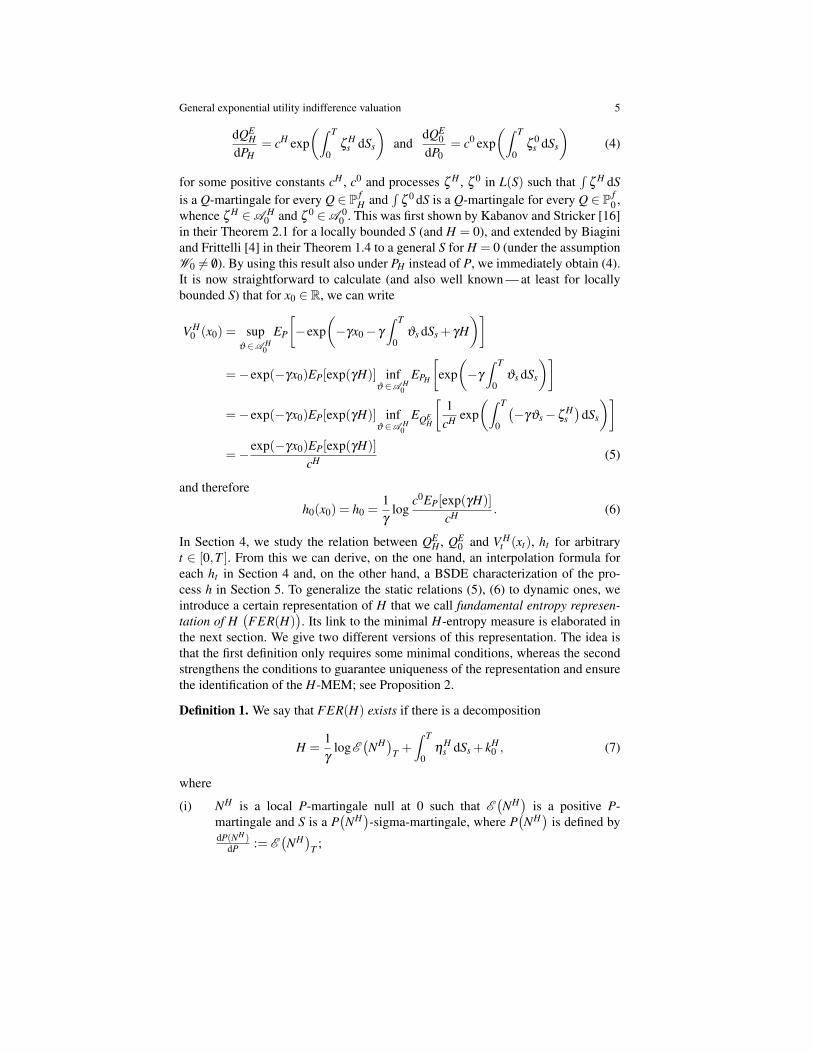
We briefly recall the relation between QEH , QE
0 and the indifference value h0(x0)at time 0 to motivate the definition of FER(H), which we introduce later in thissection. Assume Pe, f
H 6= /0 and Pe, f0 6= /0. The PH -density of QE
H and the P-density ofQE
0 have the form
General exponential utility indifference valuation 5
dQEH
dPH= cH exp
(∫ T
0ζ
Hs dSs
)and
dQE0
dP0= c0 exp
(∫ T
0ζ
0s dSs
)(4)
for some positive constants cH , c0 and processes ζ H , ζ 0 in L(S) such that∫
ζ H dSis a Q-martingale for every Q ∈ P f
H and∫
ζ 0 dS is a Q-martingale for every Q ∈ P f0 ,
whence ζ H ∈A H0 and ζ 0 ∈A 0
0 . This was first shown by Kabanov and Stricker [16]in their Theorem 2.1 for a locally bounded S (and H = 0), and extended by Biaginiand Frittelli [4] in their Theorem 1.4 to a general S for H = 0 (under the assumptionW0 6= /0). By using this result also under PH instead of P, we immediately obtain (4).It is now straightforward to calculate (and also well known — at least for locallybounded S) that for x0 ∈ R, we can write
V H0 (x0) = sup
ϑ ∈A H0
EP
[−exp
(−γx0− γ
∫ T
0ϑs dSs + γH
)]=−exp(−γx0)EP[exp(γH)] inf
ϑ ∈A H0
EPH
[exp(−γ
∫ T
0ϑs dSs
)]=−exp(−γx0)EP[exp(γH)] inf
ϑ ∈A H0
EQEH
[1
cH exp(∫ T
0
(−γϑs−ζ
Hs)
dSs
)]=−exp(−γx0)EP[exp(γH)]
cH (5)
and therefore
h0(x0) = h0 =1γ
logc0EP[exp(γH)]
cH . (6)
In Section 4, we study the relation between QEH , QE
0 and V Ht (xt), ht for arbitrary
t ∈ [0,T ]. From this we can derive, on the one hand, an interpolation formula foreach ht in Section 4 and, on the other hand, a BSDE characterization of the pro-cess h in Section 5. To generalize the static relations (5), (6) to dynamic ones, weintroduce a certain representation of H that we call fundamental entropy represen-tation of H
(FER(H)
). Its link to the minimal H-entropy measure is elaborated in
the next section. We give two different versions of this representation. The idea isthat the first definition only requires some minimal conditions, whereas the secondstrengthens the conditions to guarantee uniqueness of the representation and ensurethe identification of the H-MEM; see Proposition 2.
Definition 1. We say that FER(H) exists if there is a decomposition
H =1γ
logE(NH)
T +∫ T
0η
Hs dSs + kH
0 , (7)
where
(i) NH is a local P-martingale null at 0 such that E(NH)
is a positive P-martingale and S is a P
(NH)-sigma-martingale, where P
(NH)
is defined bydP(NH )
dP := E(NH)
T ;

6 Christoph Frei and Martin Schweizer
(ii) ηH is in L(S) and such that∫ T
0 ηHs dSs ∈ L1
(P(NH))
;(iii) kH
0 ∈ R is constant.
In this case, we say that(NH ,ηH ,kH
0)
is an FER(H). If moreover∫ T
0η
Hs dSs ∈ L1(Q) and EQ
[∫ T
0η
Hs dSs
]≤ 0 for all Q ∈ P f
H
and∫
ηH dS is a P
(NH)-martingale,
(8)
we say that(NH ,ηH ,kH
0)
is an FER?(H). For any FER(H)(NH ,ηH ,kH
0), we set
kHt := kH
0 +1γ
logE(NH)
t +∫ t
0η
Hs dSs for t ∈ [0,T ] (9)
and call P(NH)
the probability measure associated with(NH ,ηH ,kH
0).
Because E(NH)
is by (i) a positive P-martingale, the local P-martingale NH hasno negative jumps whose absolute value is 1 or more, and P
(NH)
is a probabilitymeasure equivalent to P. We consider two FER(H)
(NH ,ηH ,kH
0)
and(NH , ηH , kH
0)
as equal if NH and NH are versions of each other (hence indistinguishable, sinceboth are RCLL),
∫ηH dS is a version of
∫ηH dS, and kH
0 = kH0 . For future use, we
note that (7) and (9) combine to give
H = kHt +
1γ
logE(NH)
t,T +∫ T
tη
Hs dSs for t ∈ [0,T ]. (10)
The next result shows that for continuous asset prices, we can write FER(H)in a different (and perhaps more familiar) form. For its formulation, we need thefollowing definition. We say that S satisfies the structure condition (SC) if
Si = Si0 +Mi +
d
∑j=1
∫λ
j d〈Mi,M j〉, i = 1, . . . ,d,
where M is a locally square-integrable local P-martingale null at 0 and λ isa predictable process such that the (final value of the) mean-variance tradeoff,KT = ∑
di, j=1
∫ T0 λ i
sλj
s d〈Mi,M j〉s = 〈∫
λ dM〉T , is almost surely finite.
Proposition 1. Assume that S is continuous. Then a triple(NH ,ηH ,kH
0)
is anFER(H) if and only if S satisfies (SC) and NH = NH +
∫λ dM, ηH = ηH − 1
γλ ,
kH0 = kH
0 satisfy
H =1γ
logE(NH)
T +∫ T
0η
Hs dSs +
12γ
⟨∫λ dM
⟩T
+ kH0 (11)
and

General exponential utility indifference valuation 7
(i′) NH is a local P-martingale null at 0 and strongly P-orthogonal to each com-ponent of M, and E
(NH)E(−∫
λ dM)
is a positive P-martingale;(ii′) ηH is in L(S) and such that
∫ T0(ηH
s + 1γλs)
dSs is P(NH)-integrable, where
dP(NH )dP := E
(NH)
T E(−∫
λ dM)
T ;(iii′) kH
0 ∈ R is constant.
Proof. Let first(NH ,ηH ,kH
0)
be an FER(H). Its associated measure P(NH)
isequivalent to P and S is a local P
(NH)-martingale since S is continuous. By The-
orem 1 of Schweizer [23], S satisfies (SC) and we can write NH = NH −∫
λ dM,where NH is a local P-martingale null at 0 and strongly P-orthogonal to eachcomponent of M, and E
(NH)
= E(NH)E(−∫
λ dM). The last equality uses that[
NH ,∫
λ dM]= 0 due to the continuity of M. Hence conditions (i)–(iii) of FER(H)
imply (i′)–(iii′), and (7) is equivalent to (11) by (SC) and the continuity of S.Conversely, let
(NH , ηH , kH
0)
be as in the proposition. We claim that the triple(NH−
∫λ dM, ηH + 1
γλ , kH
0)
is an FER(H). Because M is a local P-martingale and
E(NH)
= E(NH)E(−∫
λ dM)
is the P-density process of P(NH), the process L
defined byLt := Mt −
⟨NH ,M
⟩t , t ∈ [0,T ]
is a local P(NH)-martingale by Girsanov’s theorem; see for instance Theorem III.40
of Protter [21] and observe that⟨E(NH),M⟩
=∫
E(NH)−d⟨NH ,M
⟩exists since M
is continuous like S. Because NH is strongly P-orthogonal to each component of Mand M is continuous, we have
⟨NH ,Mi⟩=
⟨NH −
∫λ dM,Mi
⟩=−
d
∑j=1
∫λ
j d〈M j,Mi〉, i = 1, . . . ,d,
and so (SC) shows that S = L + S0 is also a local P(NH)-martingale. The other
conditions of FER(H) are easy to check. ut
Remark 1. 1) Suppose that S is continuous and satisfies (SC). If the stochastic expo-nential E
(−∫
λ dM)
is a P-martingale, conditions (i′) and (ii′) in Proposition 1 canbe written under the probability measure P defined by dP
dP := E(−∫
λ dM)
T , whichis called the minimal local martingale measure in the terminology of Follmer andSchweizer [9]. This means that condition (i′) in Proposition 1 is equivalent to
(i′′) NH is a local P-martingale null at 0 and strongly P-orthogonal to each com-ponent of S, and E
(NH)
is a positive P-martingale,
and P(NH)
can be defined by dP(NH )dP
:= E(NH)
T . To prove the equivalence of(i′) and (i′′), first assume that NH is a local P-martingale null at 0 and strongly P-orthogonal to each Mi. Then[
NH ,∫
λ dM]
=⟨
NH ,∫
λ dM⟩
= 0

8 Christoph Frei and Martin Schweizer
by the continuity of M, and hence NH is also a local P-martingale by Girsanov’stheorem; see, for instance, Theorem III.40 of Protter [21]. The continuity of S, (SC)and the strong P-orthogonality of NH to M entail[
NH ,Si]
=⟨
NH ,Mi⟩
= 0, i = 1, . . . ,d,
implying that NH is strongly P-orthogonal to each component of S. The proof of“(i′′) =⇒ (i′)” goes analogously.
2) Assume that S is not necessarily continuous but locally bounded and satisfies(SC) with λ i ∈ L2
loc
(Mi), i = 1, . . . ,d, and let
(NH ,ηH ,kH
0)
be an FER(H). Thenwe can still write NH = NH −
∫λ dM for a local P-martingale NH null at 0 and
strongly P-orthogonal to each component of M, by using Girsanov’s theorem, (SC)and the fact that E
(NH)
defines an equivalent local martingale measure. However,we cannot separate E
(NH −
∫λ dM
)into two factors. ♦
3 No-arbitrage and existence of FER(H)
Theorem 1 below says that a certain notion of no-arbitrage is equivalent to the exis-tence of FER(H). It can be considered as an exponential analogue to the L2-resultof Theorem 3 in Bobrovnytska and Schweizer [5]. For a locally bounded S, the im-plication “=⇒” roughly corresponds to Proposition 2.2 of Becherer [1], who makesuse of the idea to consider known results under PH instead of P. This technique,which already appears in Delbaen et al. [6], will also be central for the proofs of ourTheorem 1 and Proposition 2.
We start with a result that gives sufficient conditions for WH ⊆W0 and Pe, f0 ⊆ Pe, f
H
as well as for W0 = WH and Pe, f0 = Pe, f
H . The relation between Pe, f0 and Pe, f
H will beused later, while W0 = WH is helpful in applications to verify the condition (1).
Lemma 1. If H satisfies
EP[exp(−εH)
]< ∞ for some ε > 0, (12)
then WH ⊆W0, P f0 ⊆ P f
H and Pe, f0 ⊆ Pe, f
H . If H satisfies
EP[exp((γ + ε)H
)]< ∞ and EP
[exp(−εH)
]< ∞ for some ε > 0, (13)
then W0 = WH , P f0 = P f
H and Pe, f0 = Pe, f
H .
Proof. We first show WH ⊆W0 under (12). For c > 0, Holder’s inequality yields

General exponential utility indifference valuation 9
EP[exp(cW )
]= EP
[exp(
cW +εγ
ε + γH)
exp(− εγ
ε + γH)]
≤(
EP
[exp(
ε + γ
εcW + γH
)]) εε+γ (
EP[exp(−εH)
]) γ
ε+γ
(14)
=(
EPH
[exp(
ε + γ
εcW)]
EP[exp(γH)
]) εε+γ (
EP[exp(−εH)
]) γ
ε+γ
.
Because of EP[exp(γH)
]< ∞ and (12), this is finite if W ∈WH , and then W ∈W0.
To prove W0 = WH under (13), we only need to show W0 ⊆ WH . For c > 0 andW ∈W0, we obtain similarly to (14) that
EPH
[exp(cW )
]≤(EP[exp((ε + γ)H
)]) γ
ε+γ
EP[exp(γH)]
(EP
[exp(
ε + γ
εcW)]) ε
ε+γ
< ∞
by (13), and hence W ∈WH .The remainder of the second part follows from Lemma A.1 in Becherer [1]. The
proof of the rest of the first part is very similar. Indeed, (12) and the standing as-sumption that EP
[exp(γH)
]< ∞ imply EP
[exp(ε|H|
)]< ∞, where ε := min(ε,γ).
Lemma 3.5 of Delbaen et al. [6] yields
EQ[ε|H|
]≤ I(Q|P)+
1e
EP[exp(ε|H|
)]for Q P. (15)
If Q ∈ P f0 , the right-hand side is finite, thus EQ
[|H|]< ∞, and we have
I(Q|PH) = EQ
[log
dQdP− log
dPH
dP
]= I(Q|P)+ logEP
[exp(γH)
]− γEQ[H],
which is finite. This shows Q ∈ P fH , and Pe, f
0 ⊆ Pe, fH follows analogously. ut
Theorem 1. We have that
Pe, fH 6= /0 ⇐⇒ FER?(H) exists ⇐⇒ FER(H) exists.
In particular, if Pe, f0 6= /0 and H satisfies (12), then FER?(H) exists.
Proof. We first show that Pe, fH 6= /0 yields the existence of FER?(H). As already
mentioned, Pe, fH 6= /0 (and the standing assumption WH 6= /0) imply by Proposition 3
and Remarks 2, 3 of Biagini and Frittelli [3], applied to PH instead of P, existenceand uniqueness of the H-MEM QE
H ∈ Pe, fH . Using QE
H ≈ PH ≈ P, we can write
dQEH
dP= E
(NH)
T (16)
for some local P-martingale NH null at 0 such that E(NH)
is a positive P-martingaleand S is a QE
H -sigma-martingale. Moreover, by Theorem 1.4 of Biagini and Frit-

10 Christoph Frei and Martin Schweizer
telli [4], applied to PH instead of P, we have as in (4)
dQEH
dPH= cH exp
(∫ T
0ζ
Hs dSs
)(17)
for a constant cH > 0 and some ζ H in L(S) such that∫
ζ H dS is a Q-martingale forevery Q∈ P f
H . Since dPHdP = exp(γH)
/EP[exp(γH)
], comparing (17) with (16) gives
E(NH)
T = cH1 exp
(∫ T
0ζ
Hs dSs + γH
),
where cH1 := cH
/EP[exp(γH)
]is a positive constant. We thus obtain
H =1γ
logE(NH)
T −1γ
∫ T
0ζ
Hs dSs + cH
2 with cH2 :=−1
γlogcH
1 ,
and hence(NH ,− 1
γζ H,cH
2)
is an FER?(H). Note that∫
ζ H dS is a P(NH)-martin-
gale because the H-MEM QEH equals the probability measure P
(NH)
associatedwith
(NH ,− 1
γζ H ,cH
2)
by construction; compare (16).To establish the equivalences of Theorem 1, it remains to show that the existence
of FER(H) implies Pe, fH 6= /0, because every FER?(H) is obviously an FER(H).
So let(NH ,ηH ,kH
0)
be an FER(H) and recall that its associated measure P(NH)
is defined by dP(NH )dP := E
(NH)
T . We prove that P(NH)∈ Pe, f
H . By condition (i) onFER(H), P
(NH)
is a probability measure equivalent to P and S is a P(NH)-sigma-
martingale. To show that P(NH)
has finite relative entropy with respect to PH , wewrite
dP(NH)dPH
=dP(NH)
dPdP
dPH= E
(NH)
T exp(−γH)EP[exp(γH)
]= exp
(−γkH
0)EP[exp(γH)
]exp(−γ
∫ T
0η
Hs dSs
), (18)
where the last equality is due to the decomposition (7) in FER(H). This yields by(ii) of FER(H) that
I(
P(NH)∣∣∣PH
)= EP(NH )
[log
dP(NH)dPH
]=−γkH
0 + logEP[exp(γH)
]− γEP(NH )
[∫ T
0η
Hs dSs
]< ∞.
Finally, the last assertion follows directly from the first part of Lemma 1. ut

General exponential utility indifference valuation 11
While the existence of FER(H) and of FER?(H) is equivalent by Theorem 1, thetwo representations are obviously different since FER?(H) imposes more stringentconditions. The next result serves to clarify this difference.
Proposition 2. Assume Pe, fH 6= /0 and let
(NH ,ηH ,kH
0)
be an FER(H) with associ-ated measure P
(NH). Then the following are equivalent:
(a)(NH ,ηH ,kH
0)
is an FER?(H), i.e.,(NH ,ηH ,kH
0)
satisfies (8);(b) P
(NH)
equals the H-MEM QEH , and
∫ηH dS is a P
(NH)-martingale;
(c)∫
ηH dS is a QEH -martingale and EP(NH )
[∫ T0 ηH
s dSs]= 0;
(d)∫
ηH dS is a Q-martingale for every Q ∈ P fH .
Moreover, the class of FER?(H) consists of a singleton.
Proof. Clearly, (d) implies (a), and also (c) since QEH exists by Proposition 3 of
Biagini and Frittelli [3], using Pe, fH 6= /0 and the standing assumption WH 6= /0. We
prove “(a) =⇒ (b)”, “(c) =⇒ (b)” and finally “(b) =⇒ (d)”. The first implicationgoes as in the proof of Theorem 2.3 of Frittelli [11], because we have by (18) that
dP(NH)dPH
= cH3 exp
(−γ
∫ T
0η
Hs dSs
)with cH
3 := exp(−γkH
0)EP[exp(γH)
]. (19)
The implication “(c) =⇒ (b)” follows from the first part of the proof of Proposi-tion 3.2 of Grandits and Rheinlander [12], which does not use the assumption that Sis locally bounded. To show “(b) =⇒ (d)”, note that (b), (17) and (19) yield
cH3 exp
(−γ
∫ T
0η
Hs dSs
)= cH exp
(∫ T
0ζ
Hs dSs
)P-a.s., (20)
where ζ H in L(S) is such that∫
ζ H dS is a Q-martingale for every Q ∈ P fH . Tak-
ing logarithms and P(NH)-expectations in (20), we obtain cH
3 = cH by using thatP(NH)∈ Pe, f
H by the proof of Theorem 1. Thus∫ T
0 ηHs dSs = − 1
γ
∫ T0 ζ H
s dSs P-a.s.and hence
∫ηH dS =− 1
γ
∫ζ H dS since both
∫ηH dS and
∫ζ H dS are P
(NH)-martin-
gales. Therefore,∫
ηH dS =− 1γ
∫ζ H dS is a Q-martingale for every Q ∈ P f
H .
Theorem 1 implies the existence of FER?(H) because Pe, fH 6= /0. To show unique-
ness, let(NH ,ηH ,kH
0)
and(NH , ηH , kH
0)
be two FER?(H). Since the minimal H-entropy measure is unique by Proposition 3 of Biagini and Frittelli [3], we havefrom “(a) =⇒ (b)” that
E(NH)
T =dQE
HdP
= E(NH)
T .
So E(NH)
is a version of E(NH)
since both are P-martingales, and taking stochasticlogarithms implies that NH is a version of NH . Similarly, (19) and (c) yield
−γkH0 + log
(EP[exp(γH)
])= EQE
H
[log
dQEH
dPH
]=−γ kH
0 + log(
EP[exp(γH)
]),

12 Christoph Frei and Martin Schweizer
thus kH0 = kH
0 , and therefore again from (19) that∫ T
0η
Hs dSs =−1
γlog(
1cH
3
dQEH
dPH
)=∫ T
0η
Hs dSs.
But both∫
ηH dS and∫
ηH dS are QEH -martingales due to (d), and so
∫ηH dS is a
version of∫
ηH dS. ut
Remark 2. Exploiting Proposition 3.4 of Grandits and Rheinlander [12], applied toPH instead of P, gives a sufficient condition for FER?(H) by using our Proposi-tion 2. Indeed, assume that S is locally bounded and Pe, f
H 6= /0. If for an FER(H)(NH ,ηH ,kH
0),∫
ηH dS is a BMO(P(NH))
-martingale and EPH
[∣∣∣ dP(NH )dPH
∣∣∣−ε]< ∞
for some ε > 0, then(NH ,ηH ,kH
0)
is the FER?(H).Another sufficient criterion is obtained from Proposition 3.2 of Rheinlander [22]
in view of our Proposition 2. Namely, if S is locally bounded and for an FER(H)(NH ,ηH ,kH
0)
there exists ε > 0 such that EPH
[exp(
ε[∫
ηH dS]
T
)]< ∞, then(
NH ,ηH ,kH0)
is the FER?(H). ♦
While there is always at most one FER?(H) by Proposition 2, the next exampleshows that there may be several FER(H). This also illustrates that the uniquenessfor FER?(H) is closely related to integrability properties.
Example 1. Take two independent P-Brownian motions W and W⊥, denote by Ftheir P-augmented filtration and choose d = 1, S = W and H ≡ 0. The MEM QE
0then equals P since S is a P-martingale, and (0,0,0) is the unique FER?(0).
To construct another FER(0), choose N0 := W⊥. Then E(N0)
= E(W⊥)
isclearly a positive P-martingale strongly P-orthogonal to S = W so that condition (i)in FER(0) holds. Define P
(N0)
as usual by dP(N0)dP := E
(N0)
T = E(W⊥)
T . ByGirsanov’s theorem, W and W⊥t := W⊥t − t, 0 ≤ t ≤ T , are then P
(N0)-Brownian
motions and we can explicitly compute
EP
[logE
(N0)
T
]= EP
[W⊥T −T/2
]=−T/2,
I(
P(N0)∣∣∣P)= EP(N0)
[logE
(N0)
T
]= EP(N0)
[W⊥T +T/2
]= T/2. (21)
This shows that P(N0)∈ Pe, f
0 . Since S = W is a P-Brownian motion, Proposition 1of Emery et al. [8] now yields for every c ∈ R a process η0(c) in L(S) such that
−1γ
logE(W⊥)
T − c =∫ T
0η
0s (c)dSs P-a.s. (22)
Because I(P(N0)∣∣P) < ∞, using the inequality x| logx| ≤ x logx + 2e−1 shows
that∫ T
0 η0s (c)dSs is in L1
(P(N0))
so that (ii) of FER(0) is also satisfied. Hence(N0,η0(c),c
)is an FER(0), but does not coincide with (0,0,0) which is the

General exponential utility indifference valuation 13
FER?(0). To check that property (8) indeed fails, we can easily see from (21) and(22) that
∫η0(c)dS cannot be a P
(N0)-martingale if c 6= − 1
2γT . If c = − 1
2γT , we
can simply compute, for P ∈ P f0 , that
EP
[∫ T
0η
0s (c)dSs
]=−1
γEP
[logE
(N0)
T
]+
12γ
T =1γ
T > 0.
We have just constructed an FER(0) different from FER?(0). Yet anotherFER(0) can be obtained by choosing for k ∈ R\0 a process β 0(k) in L(S) suchthat ∫ T/2
0β
0s (k)dSs = k and
∫ T
T/2β
0s (k)dSs =−k P-a.s.,
which is possible by Proposition 1 of Emery et al. [8]. Clearly,∫ T
0 β 0s (k)dSs = 0
P-a.s. and(0,β 0(k),0
)is an FER(0) (with associated measure P), which even sat-
isfies EQ[∫ T
0 β 0s (k)dSs
]= 0 for all Q ∈ P f
0 ; but∫
β 0(k)dS is not a P-martingale.This ends the example. ♦
Example 1 shows that we should focus on FER?(H) if we want to obtain goodresults. If S is continuous and we impose additional assumptions, the next resultgives BMO-properties for the components of FER?(H). This will be used later whenwe give a BSDE description for the exponential utility indifference value process.We first recall some definitions.
Let Q be a probability measure on (Ω ,F ) equivalent to P and p > 1. An adaptedpositive RCLL stochastic process Z is said to satisfy the reverse Holder inequalityRp(Q) if there exists a positive constant C such that
ess supτ stopping
time
EQ
[(ZT
Zτ
)p∣∣∣∣∣Fτ
]= ess sup
τ stoppingtime
EQ[(Zτ,T )p∣∣Fτ
]≤C.
Recall that Zτ,T = ZT /Zτ for a positive process Z. We say that Z satisfies the reverseHolder inequality RL logL(Q) if there exists a positive constant C such that
ess supτ stopping
time
EQ[Zτ,T log+ Zτ,T |Fτ ]≤C.
Z satisfies condition (J) if there exists a positive constant C such that
1C
Z− ≤ Z ≤CZ−.
Theorem 2. Assume that S is continuous, H is bounded and there exists Q ∈ Pe, f0
whose P-density process satisfies RL logL(P). Let(NH ,ηH ,kH
0)
be an FER(H). Thenthe following are equivalent:
(a)(NH ,ηH ,kH
0)
is the FER?(H);

14 Christoph Frei and Martin Schweizer
(b) NH is a BMO(P)-martingale, E(NH)
satisfies condition (J), and∫
ηH dS is aP(NH)-martingale;
(c) NH is a BMO(P)-martingale, E(NH)
satisfies condition (J), and∫
ηH dS is aBMO
(P(NH))
-martingale;(d)
∫ηH dM is a BMO(P)-martingale, where M is the P-local martingale part
of S;(e) there exists ε > 0 such that EP
[exp(
ε[∫
ηH dS]
T
)]< ∞.
The hypotheses of Theorem 2 are for instance fulfilled if H is bounded, S iscontinuous and satisfies (SC), and
∫λ dM is a BMO(P)-martingale. To see this,
note that E(−∫
λ dM)
then satisfies the reverse Holder inequality Rp(P) for somep > 1 by Theorem 3.4 of Kazamaki [18]. The fact that there exists k < ∞ such thatx logx≤ k +xp for all x > 0 now implies that E
(−∫
λ dM)
also satisfies RL logL(P).Hence the minimal local martingale measure P given by dP
dP := E(−∫
λ dM)
T is inPe, f
0 and its P-density process satisfies RL logL(P).
Proof of Theorem 2. By Lemma 1, Pe, fH = Pe, f
0 6= /0 so that there exists an FER(H)(NH ,ηH ,kH
0)
by Theorem 1. Before we show that (a)–(e) are equivalent, we needsome preparation. Let Q be a probability measure equivalent to P. Denoting by Zthe P-density process of Q and by Y the PH -density process of Q, we prove that
Z satisfies RL logL(P) if and only if Y satisfies RL logL(PH), (23)Z satisfies condition (J) if and only if Y satisfies condition (J). (24)
To that end, observe first that because H is bounded, there exists a positive constant kwith 1
k ≤dPHdP ≤ k, which yields
1k
Z ≤ Y ≤ kZ. (25)
For any stopping time τ , (25) implies
EPH [Yτ,T log+Yτ,T |Fτ ]≤ EP
[Zτ,T log+(Zτ,T k2)∣∣∣Fτ
],
and so the inequality log+(ab)≤ log+a+ logb for a > 0 and b≥ 1 yields
EP
[Zτ,T log+(Zτ,T k2)∣∣∣Fτ
]≤ EP[Zτ,T log+ Zτ,T |Fτ ]+2logk,
which is bounded independently of τ if Z satisfies RL logL(P). If Z satisfies condi-tion (J) with constant C, then (25) gives
Y ≤ kZ ≤ kCZ− ≤ k2CY− and Y ≥ 1k
Z ≥ 1kC
Z− ≥1
k2CY−.
So the “only if” part of both (23) and (24) is clear, and the “if” part is provedsymmetrically.
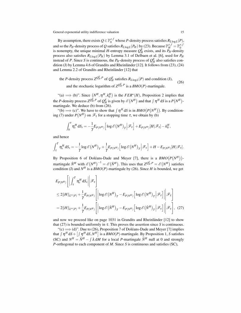
General exponential utility indifference valuation 15
By assumption, there exists Q∈Pe, f0 whose P-density process satisfies RL logL(P),
and so the PH -density process of Q satisfies RL logL(PH) by (23). Because Pe, fH = Pe, f
0is nonempty, the unique minimal H-entropy measure QE
H exists, and its PH -densityprocess also satisfies RL logL(PH) by Lemma 3.1 of Delbaen et al. [6], used for PHinstead of P. Since S is continuous, the PH -density process of QE
H also satisfies con-dition (J) by Lemma 4.6 of Grandits and Rheinlander [12]. It follows from (23), (24)and Lemma 2.2 of Grandits and Rheinlander [12] that
the P-density process ZQEH ,P of QE
H satisfies RL logL(P) and condition (J),
and the stochastic logarithm of ZQEH ,P is a BMO(P)-martingale.
(26)
“(a) =⇒ (b)”. Since(NH ,ηH ,kH
0)
is the FER?(H), Proposition 2 implies thatthe P-density process ZQE
H ,P of QEH is given by E
(NH)
and that∫
ηH dS is a P(NH)-
martingale. We deduce (b) from (26).“(b) =⇒ (c)”. We have to show that
∫ηH dS is in BMO
(P(NH))
. By condition-ing (7) under P
(NH)
on Fτ for a stopping time τ , we obtain by (b)∫τ
0η
Hs dSs =−1
γEP(NH )
[logE
(NH)
T
∣∣∣Fτ
]+EP(NH )[H|Fτ ]− kH
0 ,
and hence∫ T
τ
ηHs dSs =−1
γlogE
(NH)
T +1γ
EP(NH )
[logE
(NH)
T
∣∣∣Fτ
]+H−EP(NH )[H|Fτ ].
By Proposition 6 of Doleans-Dade and Meyer [7], there is a BMO(P(NH))
-
martingale NH with E(NH)−1 = E
(NH). This uses that ZQE
H ,P = E(NH)
satisfiescondition (J) and NH is a BMO(P)-martingale by (26). Since H is bounded, we get
EP(NH )
[∣∣∣∣∫ T
τ
ηHs dSs
∣∣∣∣∣∣∣∣∣Fτ
]
≤ 2‖H‖L∞(P) +1γ
EP(NH )
[∣∣∣∣ logE(NH)
T −EP(NH )
[logE
(NH)
T
∣∣∣Fτ
]∣∣∣∣∣∣∣∣∣Fτ
]
= 2‖H‖L∞(P) +1γ
EP(NH )
[∣∣∣∣ logE(NH)
T −EP(NH )
[logE
(NH)
T
∣∣∣Fτ
]∣∣∣∣∣∣∣∣∣Fτ
], (27)
and now we proceed like on page 1031 in Grandits and Rheinlander [12] to showthat (27) is bounded uniformly in τ . This proves the assertion since S is continuous.
“(c) =⇒ (d)”. Due to (26), Proposition 7 of Doleans-Dade and Meyer [7] impliesthat
∫ηH dS+
[∫ηH dS,NH
]is a BMO(P)-martingale. By Proposition 1, S satisfies
(SC) and NH = NH −∫
λ dM for a local P-martingale NH null at 0 and stronglyP-orthogonal to each component of M. Since S is continuous and satisfies (SC),
16 Christoph Frei and Martin Schweizer[∫η
H dS,NH]
=[∫
ηH dM,NH
]=−
[∫η
H dM,∫
λ dM]
=−d
∑i, j=1
∫ (η
H)iλ
j d〈Mi,M j〉.
Hence∫
ηH dS +[∫
ηH dS,NH]=∫
ηH dM is a BMO(P)-martingale.“(d) =⇒ (e)”. We set
ε :=1
2‖∫
ηH dM‖2BMO2(P)
and L :=√
ε
∫η
H dM.
Clearly, L is like∫
ηH dM a continuous BMO(P)-martingale and we have that‖L‖BMO2(P) = 1
/√2 < 1. Since S is continuous, the John-Nirenberg inequality
(see
Theorem 2.2 of Kazamaki [18])
yields
EP
[exp
(ε
[∫η
H dS]
T
)]= EP
[exp([L]T
)]≤ 1
1−‖L‖2BMO2(P)
< ∞.
“(e) =⇒ (a)”. This is based on the same idea as the proof of Proposition 3.2 ofRheinlander [22]. Lemma 3.5 of Delbaen et al. [6] yields
EQ
[ε
[∫η
H dS]
T
]≤ I(Q|PH)+
1e
EPH
[exp
(ε
[∫η
H dS]
T
)]< ∞
for any Q ∈ P fH because H is bounded and (e) holds. So
[∫ηH dS
]T is Q-integrable
and thus the local Q-martingale∫
ηH dS is a square-integrable Q-martingale for anyQ ∈ P f
H . This concludes the proof in view of Proposition 2. ut
4 Relating FER?(H) and FER?(0) to the indifference value
In this section, we establish the connection between FER?(H), FER?(0) and theindifference value process h. We then derive and study an interpolation formulafor h. Throughout this section, we assume that
Pe, fH 6= /0 and Pe, f
0 6= /0,
and we denote by(NH ,ηH ,kH
0)
and(N0,η0,k0
0)
the unique FER?(H) and FER?(0)with associated measures P
(NH)
= QEH and P
(N0)
= QE0 , respectively.
Our first result expresses the maximal expected utility and the indifference valuein terms of the given FER?(H) and FER?(0). For a locally bounded S, this is verysimilar to Becherer [1]; see in particular there Propositions 2.2 and 3.5 and thediscussion on page 12 at the end of Section 3. Indeed, the main differences are that

General exponential utility indifference valuation 17
the representation in [1] is given in terms of certainty equivalents instead of maximalconditional expected utilities and S is locally bounded; but the results are the same.
Theorem 3. V H , V 0 and h are well defined and, for any t ∈ [0,T ] and any Ft -measurable random variable xt , we have
V Ht (xt) =−exp
(−γxt + γkH
t)
(28)
andht(xt) = ht = kH
t − k0t , (29)
where kHt (and k0
t , with the obvious adaptations) are defined in (9).
Proof. Let us first write (2) as
V Ht (xt) =−exp(−γxt) ess inf
ϑ ∈A Ht
ϕHt (ϑ) (30)
with the abbreviation
ϕHt (ϑ) := EP
[exp(−γ
∫ T
tϑs dSs + γH
)∣∣∣∣Ft
].
Because(NH ,ηH ,kH
0)
is the FER?(H), ϕHt (ϑ) can be written by (10) as
ϕHt (ϑ) = exp
(γkH
t)EP
[E(NH)
t,T exp(
γ
∫ T
t
(η
Hs −ϑs
)dSs
)∣∣∣∣Ft
]= exp
(γkH
t)EP(NH )
[exp(
γ
∫ T
t
(η
Hs −ϑs
)dSs
)∣∣∣∣Ft
],
(31)
using Bayes’ formula. Since P(NH)= QE
H ∈ Pe, fH and
∫ϑ dS is a Q-supermartingale
and∫
ηH dS is a Q-martingale for every Q ∈ Pe, fH , we have
EP(NH )
[∫ T
t
(η
Hs −ϑs
)dSs
∣∣∣∣Ft
]≥ 0
which implies ϕHt (ϑ) ≥ exp
(γkH
t)
by Jensen’s inequality and (31). On the otherhand, the choice
ϑ?s := η
Hs , s ∈ (t,T ], (32)
gives ϕHt (ϑ ?) = exp
(γkH
t)
by (31). Because∫
ϑ ? dS =∫
ηH dS is a Q-martingalefor every Q ∈ Pe, f
H , ϑ ? is in A Ht , and (28) now follows from (30).
By the same reasoning as for (28), we obtain
V 0t (xt) =−exp
(−γxt + γk0
t).
Solving the implicit equation (3) for ht(xt) then immediately leads to (29). ut
18 Christoph Frei and Martin Schweizer
The proof of Theorem 3, especially (32), gives an interpretation for the FER?(H).An investor who must pay out the claim H at time T uses, under exponential utilitypreferences, the decomposition (7). The portion of H that he hedges by trading inS is
∫ T0 ηH
s dSs, whereas 1γ
logE(NH)
T remains unhedged. Moreover, the proof ofTheorem 3 shows that for t ∈ [0,T ] and an Ft -measurable xt , the value of V H
t (xt) isnot affected if we restrict the set A H
t to those ϑ ∈A Ht such that
∫ϑ dS is not only
a Q-supermartingale, but a Q-martingale for every Q ∈ Pe, fH .
Proposition 3. Assume that H satisfies (12). Then for any Q ∈ P f0 and t ∈ [0,T ],
ht = EQ[H|Ft ]−1γ
EQ
[log
E(NH)
t,T
E(N0)
t,T
∣∣∣∣∣Ft
]. (33)
In particular,
h0 = EQ[H]+1γ
(I(Q∣∣QE
H)− I(Q∣∣QE
0))
. (34)
The decomposition (34) of the indifference value h0 can be described as follows.The first term, EQ[H], is the expected payoff under a measure Q ∈ P f
0 . This is linearin the number of claims. The second term is a nonlinear correction term or safetyloading. It can be interpreted as the difference of the distances from QE
H and QE0 to
Q(although I(·|·) is not a metric
). This correction term is not based on all of H,
but only on the processes NH and N0 from the FER?(H) and FER?(0), i.e., on theunhedged parts of H and 0, respectively. A similar decomposition also appears forindifference pricing under quadratic preferences; see Schweizer [24].
If H satisfies (12), then the indifference value process h is a QE0 -supermartingale.
In fact, Jensen’s inequality and (33) with Q = QE0 yield ht ≥ EQE
0[H|Ft ] P-a.s. for
t ∈ [0,T ] and so h−t ∈ L1(QE
0)
since H is QE0 -integrable due to (12); compare (15).
Moreover, Z := E(NH)/
E(N0)
is a QE0 -martingale as it is the QE
0 -density processof QE
H . Thus logZ has the QE0 -supermartingale property by Jensen’s inequality, and
so has h since ht = EQE0[H|Ft ]− 1
γEQE
0[logZT |Ft ]+ 1
γlogZt for t ∈ [0,T ] by (33).
Now EQE0[ht ]≤ h0 < ∞ shows that ht is QE
0 -integrable for every t ∈ [0,T ].
Proof of Proposition 3. Since Q∈ P f0 ⊆ P f
H by Lemma 1,∫
ηH dS is a Q-martingaleby Proposition 2. Moreover, H is Q-integrable due to (12); compare (15). From (10),we thus obtain for t ∈ [0,T ] that
kHt = EQ
[H− 1
γlogE
(NH)
t,T
∣∣∣∣Ft
]. (35)
Plugging (35) and the analogous expression for k0t into (29) leads to (33).
To prove (34), we first show that I(Q∣∣QE
0)
is finite. We can write
I(Q∣∣QE
0)
= EQ
[log
dQdP
+ logdP
dQE0
]= I(Q|P)−EQ
[logE
(N0)
T
]< ∞ (36)

General exponential utility indifference valuation 19
because Q ∈ P f0 and −EQ
[logE
(N0)
T
]= γk0
0 by (35) for H = 0 and t = 0. More-over, Q P≈ QE
H gives dQdP > 0 Q-a.s. and thus from
dQdQE
H=
dQdP
dPdQE
H=
dQdP
1E (NH)T
Q-a.s.
that− logE
(NH)
T = logdQ
dQEH− log
dQdP
Q-a.s.,
and analogously for 0 instead of H. Hence
EQ
[− log
E(NH)
T
E(N0)
T
]= EQ
[log
dQdQE
H− log
dQdQE
0
]= I(Q∣∣QE
H)− I(Q∣∣QE
0),
where we have used (36) for the last equality. Now (34) follows from (33). ut
We next come to the announced interpolation formula for the indifference value.
Theorem 4. Let Q ∈ Pe, fH and ϕ in L(S) be such that
∫ϕ dS is a Q- and QE
H -martingale. Fix t ∈ [0,T ], denote by Z the P-density process of Q, set
ΨH
t :=exp(γH +
∫ Tt ϕs dSs
)Zt,T
(37)
and assume that Ψ Ht and logΨ H
t are Q-integrable. Then there exists an Ft -measur-able random variable δ H
t : Ω → [1,∞] such that for almost all ω ∈Ω ,
kHt (ω) =
1γ
log(
EQ
[∣∣Ψ Ht∣∣1/δ∣∣∣Ft
](ω))δ∣∣∣∣δ=δ H
t (ω), (38)
where
log(
EQ
[∣∣Ψ Ht∣∣1/δ∣∣∣Ft
](ω))δ∣∣∣∣δ=∞
:= limδ→∞
log(
EQ
[∣∣Ψ Ht∣∣1/δ∣∣∣Ft
](ω))δ
(39)
= EQ[logΨ
Ht∣∣Ft](ω)
for almost all ω ∈Ω .
In view of ht = kHt − k0
t by Theorem 3, (38) gives us a quasi-explicit formulafor the exponential utility indifference value if H is bounded and if we can find ameasure Q ∈ Pe, f
0 such that the corresponding Ψ 0t given in (37) and logΨ 0
t are Q-integrable for some predictable ϕ such that
∫ϕ dS is a Q-, QE
0 - and QEH -martingale.
For t = 0, one possible choice is the minimal 0-entropy measure QE0 which is by
(19) and Proposition 2 of the form dQE0
dP = c03 exp
(∫ T0 ζ 0
s dSs)
for a constant c03 and
a predictable process ζ 0 such that∫
ζ 0 dS is a Q-martingale for every Q ∈ P f0 . One
disadvantage of this choice is that QE0 is in general unknown; a second is that we still

20 Christoph Frei and Martin Schweizer
need to find some ϕ , and we know almost nothing about the potential candidate ζ 0.In Corollary 1, we give conditions under which the explicitly known minimal localmartingale measure P satisfies the assumptions of Theorem 4.
Proof of Theorem 4. From (10) and (37), we obtain via dQEH
dP = E(NH)
T and Bayes’formula that
exp(−γkH
t)EQ[Ψ
Ht∣∣Ft]= EQ
[E(NH)
t,T
Zt,Texp(∫ T
t
(ϕs + γη
Hs)
dSs
)∣∣∣∣∣Ft
]
= EQEH
[exp(∫ T
t
(ϕs + γη
Hs)
dSs
)∣∣∣∣Ft
]≥ exp
(EQE
H
[∫ T
t
(ϕs + γη
Hs)
dSs
∣∣∣∣Ft
])(40)
= 1
by Jensen’s inequality and because∫
ϕ dS and∫
ηH dS are QEH -martingales. Hence
kHt ≤
1γ
logEQ[Ψ
Ht∣∣Ft]. (41)
On the other hand, (35), (37) and Jensen’s inequality yield
γkHt = EQ
[γH− logE
(NH)
t,T
∣∣∣Ft
]= EQ
[logΨ
Ht − log
E(NH)
t,T
Zt,T
∣∣∣∣∣Ft
]≥ EQ
[logΨ
Ht∣∣Ft]. (42)
Consider the stochastic process f (·, ·) : [1,∞)×Ω → R defined by
f (δ ,ω) := log(
EQ
[∣∣Ψ Ht∣∣ 1
δ
∣∣∣Ft
](ω))δ
, (δ ,ω) ∈ [1,∞)×Ω .
Because |Ψ Ht |1/δ ≤ 1+Ψ H
t ∈ L1(Q) for all δ ∈ [1,∞), Lebesgue’s dominated con-vergence theorem and Jensen’s inequality for conditional expectations allow us tochoose a version of f which is continuous and nonincreasing in δ for all fixedω ∈ Ω , so that by monotonicity, the limit f (∞,ω) := limδ→∞ f (δ ,ω) exists forall ω ∈Ω . We next show that
f (∞,ω) = EQ[logΨ
Ht∣∣Ft](ω) for almost all ω ∈Ω . (43)
To ease the notation, we define g(·, ·) : [1,∞)×Ω → R by
g(δ ,ω) :=(
exp(
f (δ ,ω))) 1
δ = EQ
[∣∣Ψ Ht∣∣ 1
δ
∣∣∣Ft
](ω), (δ ,ω) ∈ [1,∞)×Ω

General exponential utility indifference valuation 21
so that f (δ ,ω) = δ logg(δ ,ω). Again since |Ψ Ht |1/δ ≤ 1 +Ψ H
t ∈ L1(Q) for allδ ∈ [1,∞), dominated convergence gives
limn→∞
g(n,ω) = 1 for almost all ω ∈Ω . (44)
For x > 1/2 we have x−1≥ logx≥ x−1−|x−1|2, from which we obtain by (44)that for almost all ω ∈Ω , there exists n0(ω) ∈ N such that
n(g(n,ω)−1
)≥ f (n,ω)≥ n
(g(n,ω)−1
)−n∣∣g(n,ω)−1
∣∣2, n≥ n0(ω). (45)
In view of (44) and (45), we get (43) if we show that
limn→∞
n(g(n,ω)−1
)= EQ
[logΨ
Ht∣∣Ft](ω) for almost all ω ∈Ω . (46)
But (46) follows from Lebesgue’s convergence theorem and
limn→∞
n(∣∣Ψ H
t∣∣ 1
n −1)
= limn→∞
n(
exp(
1n
logΨH
t
)−1)
= logΨH
t P-a.s.
if we show that n∣∣∣∣∣Ψ H
t∣∣1/n − 1
∣∣∣, n ∈ N, is dominated by a Q-integrable randomvariable. Due to ex−1≥ x for x ∈ R and
ddx
x(
a1x −1
)= a
1x
(1− 1
xloga
)−1≤ a
1x exp
(−1
xloga
)−1 = 0
for a > 0 and x > 0, it follows for a = Ψ Ht that
logΨH
t ≤ n(
exp(
1n
logΨH
t
)−1)≤Ψ
Ht −1, n ∈ N.
This gives n∣∣∣∣∣Ψ H
t∣∣1/n−1
∣∣∣≤ ∣∣ logΨ Ht∣∣+Ψ H
t ∈ L1(Q), n ∈ N, and proves (43).
Combining (41), (42) and (43) yields f (∞,ω)≤ γkHt (ω)≤ f (1,ω) for almost all
ω ∈Ω . By the intermediate value theorem, the set
∆(ω) :=
δ ∈ [1,∞]∣∣ f (δ ,ω) = γkH
t (ω)
is thus nonempty for almost all ω ∈Ω . Define δ Ht : Ω → [1,∞] by
δHt (ω) := sup∆(ω), ω ∈Ω , (47)
setting δ Ht := 1 on the P-null set ω ∈Ω |∆(ω) = /0. By continuity of f in δ , ∆(ω)
is closed in R∪+∞ for all ω ∈Ω , and we get for almost all ω ∈Ω that
f(δ
Ht (ω),ω
)= γkH
t (ω). (48)

22 Christoph Frei and Martin Schweizer
It remains to prove that the mapping ω 7→ δ Ht (ω) is Ft -measurable. Because f is
nonincreasing and due to (47) and (48), we have for any a ∈ [1,∞] thatω ∈Ω
∣∣δ Ht (ω) < a
=
ω ∈Ω∣∣ f(δ
Ht (ω),ω
)> f (a,ω)
=
ω ∈Ω∣∣γkH
t (ω) > f (a,ω)
=⋃
q∈Q
(ω ∈Ω
∣∣γkHt (ω) > q
∩
ω ∈Ω∣∣q > f (a,ω)
)up to a P-null set. The last set is in Ft because kH
t and f (a, ·) for fixed a ∈ [1,∞] areFt -measurable random variables. Since Ft is complete,
ω ∈Ω
∣∣δ Ht (ω) < a
is
in Ft for every a ∈ R∪+∞, and so δ Ht is Ft -measurable. ut
The next result provides a simplified version of Theorem 4 based on the use ofthe minimal local martingale measure P.
Corollary 1. Fix t ∈ [0,T ] and assume that H is bounded and S satisfies (SC). Sup-pose further that P given by dP
dP := E(−∫
λdM)
T is in Pe, f0 , that
∫λdS is a P-, QE
0 -and QE
H -martingale, and that the random variable
exp(−⟨∫
λ dM⟩
+12
[∫λ dM
]c)t,T
∏t<s≤T
e−λs·∆Ms
1−λs ·∆Ms
and its logarithm are P-integrable. Then there exist Ft -measurable random vari-ables δ 0
t , δ Ht : Ω → [1,∞] such that for almost all ω ∈Ω ,
ht(ω) =1γ
log(
EP
[∣∣Ψ Ht∣∣1/δ∣∣∣Ft
](ω))δ∣∣∣∣δ =δ H
t (ω)
− 1γ
log(
EP
[∣∣Ψ 0t∣∣1/δ ′
∣∣∣Ft
](ω))δ ′∣∣∣∣δ ′=δ 0
t (ω),
where we use the convention (39) and the definition
ΨH
t :=exp(γH−
∫ Tt λs dSs
)E(−∫
λdM)
t,T
=eγH exp(−
∫λ dS)t,T
E(−∫
λdM)
t,T
. (49)
Proof. We only need to check that Ψ 0t , Ψ H
t given by (49) and logΨ 0t , logΨ H
t are P-integrable as the result then follows from Theorems 3 and 4 with the choice Q := Pand ϕ :=−λ . Using the formula for the stochastic exponential and (SC), we get
Ψ0
t = exp(−⟨∫
λ dM⟩
+12
[∫λ dM
]c)t,T
∏t<s≤T
e−λs·∆Ms
1−λs ·∆Ms,
and thus Ψ 0t , logΨ 0
t ∈ L1(P)
by assumption. The same is true for Ψ Ht because H is
bounded by assumption. ut

General exponential utility indifference valuation 23
To the best of our knowledge, results like Theorem 4 and Corollary 1 have notbeen available in the literature so far. A closed-form expression for the exponen-tial utility indifference value has been known only in specific cases when the assetprices are modeled by continuous semimartingales; see for example [10] for explicitexpressions of the indifference value in two Brownian settings. There the adaptedprocess δ H , called the distortion power, is closely related to the instantaneous cor-relation between the driving Brownian motions. The model in [10] consists of arisk-free bank account and a stock S = S1 driven by a Brownian motion W . Theclaim H depends on another Brownian motion Y which has a time-dependent andfairly general instantaneous stochastic correlation ρ with W , with |ρ| uniformlybounded away from 1. Theorem 2 of [10] proves that the indifference value is of theform of Corollary 1 above, with δ H
t and δ 0t taking values between
δ t := infs∈ [t,T ]
1‖1−|ρs|2‖L∞(P)
and δ t := sups∈ [t,T ]
∥∥∥∥ 11−|ρs|2
∥∥∥∥L∞(P)
.
For small |ρ| (uniformly in s, in the L∞-norm), the claim H is almost unhedgeableand 1/δ H is nearly 1, whereas for |ρ| close to 1, the claim H is well hedgeable and1/δ H is nearly 0. So in that Brownian model, 1/δ H is closely related to some kindof distance of H from being attainable or hedgeable. In the subsequent discussion,we extend this idea to a more general setting, while we come back to the Brownianmodel in Section 6.
Consider the setting of Corollary 1 where S is (in addition) continuous and satis-fies (SC), and H is bounded. Then the P-martingale part M of S is also continuousand the mean-variance tradeoff process K = 〈
∫λ dM〉 = 〈
∫λ dS〉 is P-a.s. finite by
(SC). The quantity Ψ Ht from (49) then reduces to Ψ H
t = exp(γH − 1
2 (KT −Kt)),
and the assumptions of Corollary 1 are satisfied if KT is bounded, because∫
λ dMis then a BMO(P)-martingale. If we now even suppose that KT is deterministic, theindifference value at time 0 simplifies to
h0 =1γ
log(
EP
[exp(γH/δ
)])δ∣∣∣∣δ=δ H
0
(50)
by Corollary 1. If δ H0 < ∞, we can write
h0 =−U−1H
(EP
[UH(−H)
]), where UH(x) :=−exp
(−γx/δ
H0), x ∈ R,
which means that −h0 is a certainty equivalent of −H. Note, however, that this isdone under P, not P, and with respect to the utility function UH , not U , where UHdepends itself on the claim H. If δ H
0 = 1, then UH and U coincide and H is val-ued by the U-certainty equivalent under P. Moreover, (38) shows that we then musthave equality in (40) for t = 0, which implies that
∫ T0(γηH
s −λs)
dSs is determin-istic, hence
∫ (γηH −λ
)dS = 0. In other words, the equivalent formulation (11) of
FER(H) in Proposition 1 simplifies in this case to
24 Christoph Frei and Martin Schweizer
H =1γ
logE(NH)
T +12γ
KT + kH0 ,
which means that H consists only of a constant plus an unhedged term. This may beinterpreted as saying that H has maximal distance to attainability. On the oppositeextreme, the case δ H
0 = ∞ leads by (50) and (39) (and still under the same assump-tions) to h0 = EP[H]. Hence for δ H
0 = ∞, we get a familiar no-arbitrage value for H.In this case, (38) and (39) show that we must have equality in (42) for t = 0; henceE(NH)
= E(−∫
λ dM)
and thus (11) simplifies to
H =∫ T
0η
Hs dS +
12γ
KT + kH0 ,
showing that H is attainable. Summing up, we can interpret 1/δ H as the distanceof H from being attainable; for 1/δ H = 0 (convention: 1/∞ = 0), the distance isminimal, whereas for 1/δ H = 1, it is maximal. The following remark shows howthis idea can be made mathematically more precise.
Remark 3. Assume that S is continuous, satisfies (SC) and that KT =⟨∫
λ dM⟩
T isbounded, but not necessarily deterministic. By Theorem 4 and Corollary 1, we canattribute to any H ∈ L∞(P) a number δ (H) := δ H
0 in [1,∞] uniquely defined via (47)with Q = P and ϕ =−λ . Defining for G,H ∈ L∞(P)
G∼ H :⇐⇒ δ
(G+
12γ
KT
)= δ
(H +
12γ
KT
)gives an equivalence relation on L∞(P). We denote by D := L∞(P)
/∼ the set of
its equivalence classes and associate to each equivalence class a representative. Wefurther define the mapping d : D×D→ [0,1] for G,H ∈ D by
d(G,H) :=
∣∣∣∣∣ 1δ(G+ 1
2γKT) − 1
δ(H + 1
2γKT) ∣∣∣∣∣.
Clearly, d is a metric on D. A claim G ∈ L∞(P) is called(P-)attainable if it can be
written as G = EP[G]+∫ T
0 βs dSs for a predictable process β such that∫
β dS is a P-martingale, which is then even a BMO
(P)-martingale. If G is attainable, the FER?
of G+ 12γ
KT equals(−∫
λ dM,β + 1γλ ,EP[G]
), and so the term log E (NH )T
E (−∫
λ dM)Tvan-
ishes identically. This implies δ(G+ 1
2γKT)
= ∞ by the proof of Theorem 4, henceG∼ 0. Therefore,
d(0,H) =1
δ(H + 1
2γKT)
is a distance of H ∈ L∞(P) from attainability.The maximal value of d(0, ·) depends on the diversity of the filtration F. If S
has the predictable representation property in F in the sense that any H ∈ L∞(P) isattainable (as above), then∼ has only one equivalence class and d ≡ 0. On the other

General exponential utility indifference valuation 25
hand, suppose that there exists a nondeterministic local P-martingale N null at 0and strongly P-orthogonal to each component of S such that E (N) is a P-martingalebounded away from zero and infinity. The maximal distance to attainability is thenattained by 1
γlogE (N)T since d
(0, 1
γlogE (N)T
)= 1. ♦
5 A BSDE characterization of the indifference value process
In this section, we prove that the indifference value process h is (the first componentof) the unique solution, in a suitable class of processes, of a backward stochasticdifferential equation (BSDE). This result is similar to Becherer [2] and Mania andSchweizer [19], but obtained here in a general (not even locally bounded) semi-martingale model.
We assume throughout this section that
Pe, f0 6= /0
and denote by QE0 the minimal 0-entropy measure. Let us consider the BSDE
Γt = Γ0 +1γ
logE (L)t +∫ t
0ψs dSs, t ∈ [0,T ] (51)
with the boundary conditionΓT = H. (52)
We introduce three different notions of solutions to (51), (52).
Definition 2. We say that the triple (Γ ,ψ,L) is a solution of (51), (52) if
Si) Γ is a real-valued semimartingale;Sii) ψ is in L(S);Siii) L is a local QE
0 -martingale null at 0 such that E (L) is a positive QE0 -
martingale and S is a Q(L)-sigma-martingale, where Q(L) is defined bydQ(L)dQE
0:= E (L)T .
We call (Γ ,ψ,L) a special solution of (51), (52) if furthermore
Siv)∫
ψ dS is a Q-martingale for every Q ∈ Pe, f0 ;
Sv) EP
[E (L)T
dQE0
dP log(E (L)T
dQE0
dP
)]< ∞, i.e., the probability measure Q(L) de-
fined by dQ(L)dQE
0:= E (L)T has finite relative entropy with respect to P.
If S is locally bounded, we say that (Γ ,ψ,L) is an orthogonal solution of (51), (52)if it satisfies (51), (52), Si), Sii) and
Siii′) L is a local QE0 -martingale null at 0 and strongly QE
0 -orthogonal to everycomponent of S and such that E (L) is positive.

26 Christoph Frei and Martin Schweizer
Under the assumption that S is locally bounded,
a triple (Γ ,ψ,L) is a solution of (51), (52) if and only if
it is an orthogonal solution and E (L) is a QE0 -martingale.
(53)
To see this, note first that a locally bounded S is a Q(L)-sigma-martingale if and onlyif E (L)S is a local QE
0 -martingale, under the assumption that Q(L) is a probabilitymeasure. If (Γ ,ψ,L) is a solution, then Siii) holds and all of E (L)S, E (L) and S arelocal QE
0 -martingales. Hence E (L) is strongly QE0 -orthogonal to every component of
S, and therefore so is L. Conversely, if Siii′) holds, then E (L) is like L strongly QE0 -
orthogonal to every component of the local QE0 -martingale S. Hence E (L)S is a local
QE0 -martingale and thus S is a Q(L)-sigma-martingale if E (L) is a QE
0 -martingale.Our main result in this section is then
Theorem 5. Assume that H satisfies (13). Then the indifference value process h isthe first component of the unique special solution of the BSDE (51), (52).
Theorem 5 looks at first glance like Theorem 13 of Mania and Schweizer [19].The important difference, however, is that we do not suppose that the filtration Fis continuous, i.e., that all local P-martingales are continuous. If F is continuous,then 1
γlogE (L) = L/γ− γ
2 〈L/γ〉 and Theorem 5 corresponds to Theorem 13 of Ma-nia and Schweizer [19]. (Since H is allowed to be unbounded in Theorem 5, thereare some differences in the integrability properties.) However, recovering the latterresult in precise form and almost full strength from Theorem 5 requires some ad-ditional work which we discuss at the end of this section. The derivation in [19]uses the martingale optimality principle, the existence of an optimal strategy forthe indifference value process, and a comparison theorem for BSDEs. Our proof iscompletely different; it is based on our results for the FER?(H) and its relation tothe indifference value.
Theorem 4.4 of Becherer [2] is another similar result. Instead of a continuousfiltration, the framework in [2] has a continuous price process driven by Brownianmotions, and a filtration generated by these and a random measure allowing themodeling of non-predictable events. Again, to regain from Theorem 5 the samestatement as in Theorem 4.4 of Becherer [2], some additional work is necessary.
In Corollary 3.6 of the earlier paper [1], Becherer gives a characterization of dQEH
dQE0
in a locally bounded semimartingale model. Theorem 5 can be viewed as a dynamicextension of that result to a general semimartingale model.
Proof of Theorem 5. By Lemma 1, (13) implies that Pe, fH = Pe, f
0 6= /0, and so Theo-rem 3 and (9) yield
ht = kHt − k0
t = h0 +1γ
logE(NH)
t
E(N0)
t
+∫ t
0
(η
Hs −η
0s)
dSs, 0≤ t ≤ T,
where(NH ,ηH ,kH
0)
and(N0,η0,k0
0)
are the FER?(H) and FER?(0); see Propo-sition 2 for their properties. Then ψ := ηH − η0 is in L(S) and
∫ψ dS is a Q-
General exponential utility indifference valuation 27
martingale for every Q ∈ Pe, f0 = Pe, f
H . By Bayes’ formula, E(NH)/
E(N0)
is theQE
0 -density process of QEH , and so it is a positive QE
0 -martingale and its stochasticlogarithm L, defined by E (L) = E
(NH)/
E(N0), is a local QE
0 -martingale null at 0.
Moreover, dQ(L)dP = E (L)T
dQE0
dP = dQEH
dP shows Q(L) = QEH . Hence S is a Q(L)-sigma-
martingale and Sv) is satisfied because QEH has finite relative entropy with respect
to P. Since hT = H by definition, we see that h is the first component of a specialsolution of the BSDE (51), (52).
To prove uniqueness, let (Γ ,ψ,L) be any special solution of (51), (52). Denoteby(N0,η0,k0
0)
the unique FER?(0), and define
N := N0 +L+[N0,L
], η := η
0 +ψ and k0 := k00 +Γ0. (54)
We claim that(N,η ,k0) is the unique FER?(H). (55)
For the proof, we first note that E(N0)E (L) = E
(N0 + L +
[N0,L
])= E (N) by
Yor’s formula. Using (51), (52) and (7) for H = 0 thus yields
H =1γ
log(E(N0)
T E (L)T
)+∫ T
0
(η
0s +ψs
)dSs + k0
0 +Γ0
=1γ
logE (N)T +∫ T
0ηs dSs + k0.
Therefore (N,η ,k0) satisfies (7) for H, and it is enough to show that the assumptionson N and η for FER?(H) are fulfilled. By Bayes’ formula, E (N) = E
(N0)E (L) is a
positive P-martingale, because E(L)
is a positive QE0 -martingale by Siii) and E
(N0)
is the P-density process of QE0 . Writing next
dP(N)dQE
0=
dP(N)dP
dPdQE
0= E (N)T
/E(N0)
T = E (L)T ,
we see that P(N) = Q(L) which implies that
I(P(N)
∣∣P)= EP
[E (L)T
dQE0
dPlog(
E (L)TdQE
0dP
)]< ∞
by Sv) and that S is a P(N)-sigma-martingale by Siii). Because(N0,η0,k0
0)
is theFER?(0),
∫η dS =
∫η0 dS+
∫ψ dS is by Proposition 2 and Siv) a Q-martingale for
every Q∈ Pe, f0 = Pe, f
H , hence also for P(N) and QEH , and so (N,η ,k0) is an FER(H)
satisfying (c) from Proposition 2. This implies (55). Uniqueness of the FER?(H)and (54) now imply that Γ0, ψ are unique; so is L due to E (L) = E (N)
/E(N0), and
finally also Γ by (51). This ends the proof. ut
The above argument shows in particular a close link between the FER?(H) andthe BSDE (51), (52). Provided we have the FER?(0), we can construct FER?(H)from the special solution of (51), (52), and vice versa. This is familiar from ex-

28 Christoph Frei and Martin Schweizer
ponential utility indifference valuation; indeed, knowing FER?(0) corresponds toknowing the minimal 0-entropy measure QE
0 .
Remark 4. If S is locally bounded and H is bounded, there is another way to proveuniqueness of the first component of a special solution of the BSDE (51), (52),which we briefly sketch here. If (Γ ,ψ,L) is a special solution of (51), (52), theidea is to show that Γ equals the indifference value process h, which then yieldsthe desired uniqueness result. Let t ∈ [0,T ] and replace in the definition of A H
t thecondition that
∫ϑ dS is a Q-supermartingale for every Q ∈ Pe, f
H by assuming that itis a Q-martingale for every Q ∈ Pe, f
H . We do the analogous change for A 0t and note
that this does not affect the values of V Ht and V 0
t , as mentioned after the proof ofTheorem 3. We now apply Proposition 3 of Mania and Schweizer [19] to obtain
ht =1γ
log ess infϑ ∈A H
t
EQE0
[exp(
γH− γ
∫ T
tϑs dSs
)∣∣∣∣Ft
]. (56)
Using (51), (52) gives
γH = γΓ0 + logE (L)T + γ
∫ T
0ψs dSs = γΓt + log
E (L)T
E (L)t+ γ
∫ T
tψs dSs,
which we plug into (56) to obtain
ht = Γt +1γ
log ess infϑ ∈A H
t
EQ(L)
[exp(
γ
∫ T
t(ψs−ϑs)dSs
)∣∣∣∣Ft
]=: Γt +
1γ
logΛ ,
where the probability measure Q(L) is defined by dQ(L)dQE
0:= E (L)T . To show that
Λ = 1, we first note that Q(L) ∈ Pe, f0 by Sv), Pe, f
H = Pe, f0 by Lemma 1, and
∫ψ dS
as well as∫
ϑ dS are Q-martingales for every Q ∈ Pe, fH = Pe, f
0 by Siv) and becauseϑ ∈A H
t . Jensen’s inequality then yields Λ ≥ 1, and we obtain Λ ≤ 1 by the choiceϑ ? := ψ ∈A H
t . Note that also for this uniqueness proof, we have used the assump-tion that (Γ ,ψ,L) is a special solution of the BSDE (51), (52), i.e., that it alsosatisfies Siv), Sv). ♦
We have seen in Section 3 that the difference between FER(H) and the (unique)FER?(H) is an issue of integrability. The same thing happens here: The next ex-ample shows that the BSDE (51), (52) may have many solutions if we omit therequirement Siv)
(which corresponds to (d) in Proposition 2
).
Example 2. As in Example 1, take independent P-Brownian motions W and W⊥,their P-augmented filtration F and d = 1, S = W , H ≡ 0. Then QE
0 = P and (0,0,0)is the unique special solution of (51), (52).
As in Example 1, take N0 = W⊥ and use Proposition 1 of Emery et al. [8] to findfor any c ∈ R a process ψ(c) in L(S) such that
−1γ
logE(N0)
T − c =∫ T
0ψs(c)dSs P-a.s.

General exponential utility indifference valuation 29
If we then set Γt(c) := c+ 1γ
logE(N0)
t +∫ t
0 ψs(c)dSs for t ∈ [0,T ], we easily see asin Example 1 that
(Γ (c),ψ(c),N0
)is a solution to (51), (52) and satisfies Sv), but
not Siv). So we clearly have multiple solutions. ♦
Theorem 5 allows us to obtain a result similar to Proposition 3.
Corollary 2. Assume that H satisfies (13). Then we have for any probability mea-sure Q ∈ Pe, f
0 = Pe, fH and t ∈ [0,T ] that
ht = EQ[H|Ft ]−1γ
EQ[logE (L)t,T
∣∣Ft], (57)
where L is the third component of the unique special solution of the BSDE (51),(52). In particular,
h0 = EQE0[H]+
1γ
I(QE
0∣∣Q(L)
), (58)
where dQ(L)dQE
0:= E (L)T .
Proof. (57) follows from Theorem 5 by taking conditional Q-expectations betweent and T in (51), using (52) and Siv). (58) follows for Q = QE
0 . ut
Remark 5. Corollary 2 raises the question if one can find a probability measureQ ∈ Pe, f
0 such that the indifference value is the Q-conditional expectation of H.From (57) we see that logE (L) must then be a Q-martingale, and if we write theQE
0 -density process of Q as E (R) for some local QE0 -martingale R, Bayes’ formula
tells us that we want E (R) logE (L) to be a QE0 -martingale. Ito’s formula gives
d(E (R) logE (L)
)t = logE (L)t− dE (R)t +
E (R)t−E (L)t−
dE (L)t
+ E (R)t− d[
Lc,Rc− 12
Lc]
t
+ E (R)t−((∆Rt +1) log(1+∆Lt)−∆Lt
),
where Lc and Rc denote the continuous local QE0 -martingale parts of L and R. For
E (R) logE (L) to be a local QE0 -martingale, we must have that Rc = 1
2 Lc on Lc 6= 0and ∆Rt = ∆Lt−log(1+∆Lt )
log(1+∆Lt )on ∆Lt 6= 0. Therefore, we define R = Rc +Rd by
Rct :=
12
Lct and Rd
t := ∑0<s≤t
∆Ls− log(1+∆Ls)log(1+∆Ls)
I∆Ls 6=0−At , (59)
where A is the dual predictable projection under QE0 of the sum in (59). Note that Rd
is well defined, since ∆Ls >−1, ∆Ls 6= 0 implies that∣∣∣∣∆Ls− log(1+∆Ls)log(1+∆Ls)
∣∣∣∣≤ |∆Ls|;

30 Christoph Frei and Martin Schweizer
in fact, log(1+x)≥ x1+x for x >−1 implies that
∣∣∣ x−log(1+x)log(1+x)
∣∣∣≤ |x| for x >−1, x 6= 0.
By this construction, E (R) and E (R) logE (L) are local QE0 -martingales, but it is
not clear whether they are true QE0 -martingales. If they are and if Q defined by
dQdQE
0:= E (R)T is in Pe, f
0 , then we obtain indeed ht = EQ[H|Ft ] for all t ∈ [0,T ]. In
general, this representation is not linear in H since the probability measure Q may(via L) depend on H. Mania and Schweizer [19] showed in their Proposition 11 thata representation of this type exists if the filtration is continuous and H is bounded,in which case R = 1
2 L. ♦
Becherer [2] and Mania and Schweizer [19] show BMO-estimates for all com-ponents of the solution to the BSDE for the indifference value process h. It seemsdoubtful if one can obtain such results in our general framework here, but under amild additional assumption, we can still characterize Siv) via BMO-properties with-out being more specific about the filtration F; see Theorem 6 below.
The indifference hedging strategy β is defined as the difference of the strategieswhich attain V H
0 (h0) and V 00 (0), i.e., as that extra trading we do in the optimization
which can be attributed to the presence of a claim. If H satisfies (13), we haveβ = ηH − η0 = ψ by (32) and the proof of Theorem 5, where ψ is the secondcomponent of the unique special solution of the BSDE (51), (52). Hence it is ofparticular interest to know when
∫ψ dS is a BMO
(QE
0)-martingale.
Theorem 6. Assume that S is continuous, H is bounded and there exists Q ∈ Pe, f0
whose P-density process satisfies RL logL(P). Let (Γ ,ψ,L) be a solution of the BSDE(51), (52) which satisfies Sv). Then the following are equivalent:
(a) (Γ ,ψ,L) is the special solution of (51), (52), i.e., it also satisfies Siv);(b) L is a BMO
(QE
0)-martingale, E (L) satisfies condition (J), and
∫ψ dS is a
QE0 -martingale;
(c)∫
ψ dS is a BMO(QE
0)-martingale;
(d)∫
ψ dM is a BMO(P)-martingale, where M is the P-local martingale part of S;
(e) there exists ε > 0 such that EP
[exp(
ε[∫
ψ dS]
T
)]< ∞.
Proof. “(a) =⇒ (b)”. Denote by(NH ,ηH ,kH
0)
and(N0,η0,k0
0)
the unique FER?(H)and FER?(0). Theorem 2 implies that NH , N0 are BMO(P)-martingales and E
(NH),
E(N0)
satisfy condition (J), say with constants CH and C0. By the proof of Theo-rem 5, we have E (L) = E
(NH)/
E(N0)
and thus E (L) satisfies condition (J) with
constant CHC0. Since 1/E(N0)
is the QE0 -density process of P, E
(N0)−1 = E
(N0)
for a local QE0 -martingale N0, and so E (L) = E
(NH + N0 +
[NH , N0
])by Yor’s
formula. Due to the properties of N0 and NH , both N0 and NH +[NH , N0
]are
BMO(QE
0)-martingales by Propositions 6 and 7 of Doleans-Dade and Meyer [7],
and hence so is L = N0 +NH +[NH , N0
]. Finally,
∫ψ dS is a QE
0 -martingale by Siv).“(b) =⇒ (c)”, “(c) =⇒ (d)” and “(d) =⇒ (e)”. These go along the same lines as
the proofs of the corresponding implications in Theorem 2. Instead of (7) we take(51), (52), and we replace P
(NH)
by QE0 .
General exponential utility indifference valuation 31
“(e) =⇒ (a)”. Like for the corresponding implication in Theorem 2, we obtainthat
∫ψ dS is a square-integrable Q-martingale for any Q ∈ Pe, f
0 = Pe, fH , which im-
plies Siv). ut
Remark 6. Example 2 also shows that even if the assumptions of Theorem 6 aresatisfied, none of the equivalent statements (a)–(e) need hold. This is another wayof saying that there exist solutions of (51), (52) which are not special solutions. ♦
Corollary 3. Suppose the assumptions of Theorem 6 hold. Let (Γ ,ψ,L) be an or-thogonal solution of the BSDE (51), (52). Then (Γ ,ψ,L) is the special solution of(51), (52) if and only if both L and
∫ψ dS are BMO
(QE
0)-martingales and E (L) is
a QE0 -martingale which satisfies condition (J).
Proof. The “only if” part follows immediately from Theorem 6. For the “if” part,note first that (Γ ,ψ,L) is a solution of (51), (52) by (53). So we need only showthat (Γ ,ψ,L) satisfies Sv) in view of Theorem 6. We first prove that
∫ψ dS is
a BMO(Q(L)
)-martingale, where dQ(L)
dQE0
= E (L)T . Because 1/E (L) is the Q(L)-
density process of QE0 , it can be written as E (L)−1 = E
(L)
for a local Q(L)-martingale L which must satisfy L+ L+
[L, L]= 0 by Yor’s formula. The continuity
of S and the strong QE0 -orthogonality of L to S entail[∫
ψ dS, L]
=−[∫
ψ dS,L]
= 0.
This yields by Proposition 7 of Doleans-Dade and Meyer [7] that∫
ψ dS is aBMO
(Q(L)
)-martingale. For the second component η0 of the FER?(0), we sim-
ilarly have that∫
η0 dS is a BMO(Q(L)
)-martingale since
∫η0 dS is a BMO
(QE
0)-
martingale by Theorem 2. Because (Γ ,ψ,L) is a solution of (51), (52), we can write
logE (L)T =−γ
∫ T
0ψs dSs + γH− γΓ0,
and similarly, we have for the FER?(0)(N0,η0,k0
0)
that
logdQE
0dP
= logE(N0)
T =−γ
∫ T
0η
0s dSs− γk0
0.
Because∫ (
η0 +ψ)
dS is a BMO(Q(L)
)-martingale, we thus obtain
EQ(L)
[log(
E (L)TdQE
0dP
)]=−γΓ0− γk0
0 + γEQ(L)
[H−
∫ T
0
(η
0s +ψs
)dSs
]=−γΓ0− γk0
0 + γEQ(L)[H] < ∞
since H is bounded. Hence (Γ ,ψ,L) satisfies Sv) and we are done. ut
Corollary 3 allows us to recover Theorem 13 of Mania and Schweizer [19] fromour Theorem 5. However, this still requires some work which is done in the next
32 Christoph Frei and Martin Schweizer
two results. A similar approach can be used to recover Theorem 4.4 of Becherer [2]from our Theorem 5, but we do not detail this here. Although the following lemmais a special case of Proposition 7 of Mania and Schweizer [19], we give the proofhere as well, both for completeness and because it is quite simple in this case.
Lemma 2. Assume that the filtration F is continuous, H is bounded and let (Γ ,ψ,L)be an orthogonal solution of the BSDE (51), (52) with bounded first component Γ .Then L and
∫ψ dS are BMO
(QE
0)-martingales.
Proof. If L and∫
ψ dS are true QE0 -martingales, (51) yields by continuity of L
EQE0
[〈L〉T −〈L〉τ
∣∣Fτ
]= 2γEQE
0[Γτ −ΓT |Fτ ] for any stopping time τ. (60)
Because Γ is bounded, the right-hand side of (60) is bounded independently of τ ,and thus L is a BMO
(QE
0)-martingale. This implies that
(EQE
0
[〈L〉T
∣∣Fs])
0≤s≤T is
also a continuous BMO(QE
0)-martingale, because
EQE0
[∣∣∣〈L〉T −EQE0
[〈L〉T
∣∣Fτ
]∣∣∣∣∣∣∣Fτ
]≤ 2EQE
0
[〈L〉T −〈L〉τ
∣∣Fτ
]≤ 2‖L‖2
BMO2(QE0 )
for any stopping time τ . Taking conditional QE0 -expectations in (51) with t = T gives∫ s
0ψy dSy = EQE
0[ΓT −Γ0|Fs]−
1γ
Ls +12γ
EQE0
[〈L〉T
∣∣Fs], 0≤ s≤ T,
and so∫
ψ dS is a BMO(QE
0)-martingale as well. Note that we obtain bounds for
the BMO2(QE
0)-norms of L and
∫ψ dS that depend on Γ (and γ) alone.
For general L and∫
ψ dS, we stop at τn and apply the above argument with Treplaced by τn. Letting n→ ∞ then completes the proof. ut
A closer look at the proof of Lemma 2 shows that we did not use the property thatL is strongly QE
0 -orthogonal to S. However, this is of course necessary if we want toprove a uniqueness result. By combining Lemma 2 and Corollary 3, we obtain thefollowing sufficient conditions for the uniqueness of an orthogonal solution of (51),(52) with bounded first component.
Proposition 4. Assume that F is continuous, H is bounded, and there exists Q∈Pe, f0
whose P-density process satisfies RL logL(P). Then the indifference value process his the first component of the unique orthogonal solution of (51), (52) with boundedfirst component. Moreover, L and
∫ψ dS are BMO
(QE
0)-martingales.
Proof. By Theorem 5 and (53), h is the first component of an orthogonal solutionof (51), (52). Using the definition (3) of h and V H
t (ht) = exp(−γht)V Ht (0) easily
implies that the indifference value process h is bounded by ‖H‖L∞(P). If (Γ ,ψ,L) isany orthogonal solution of the BSDE (51), (52) with bounded Γ , then L and
∫ψ dS
are BMO(QE
0)-martingales by Lemma 2. By Corollary 3, (Γ ,ψ,L) is then a special
solution, which is unique by Theorem 5. ut
General exponential utility indifference valuation 33
Proposition 4 is almost identical to Theorem 13 in Mania and Schweizer [19];the only difference is that we have here the additional assumption that there ex-ists Q ∈ Pe, f
0 whose P-density process satisfies RL logL(P). The explanation for thisis that we actually prove more than we really need for Proposition 4. Mania andSchweizer [19] use a comparison result for BSDEs (their Theorem 8) to deducedirectly that one has uniqueness of orthogonal solutions to the BSDE within theclass of those with bounded first component. In contrast, the proof of Proposition 4actually shows that under the RL logL-condition, any solution with bounded first com-ponent is even a special solution—and then one appeals to Theorem 5 which assertsuniqueness within that class.
6 Application to a Brownian setting
In this section, we consider as a special case a model with one risky asset drivenby a Brownian motion and a claim coming from a second, correlated Brownianmotion. All processes are indexed by 0 ≤ s ≤ T . Let W and Y be two Brownianmotions with constant instantaneous correlation ρ satisfying |ρ| < 1. Choose as Fthe P-augmentation of the filtration generated by the pair (W,Y ), and denote byY = (Ys)0≤s≤T the P-augmentation of the filtration generated by Y alone.
As usual, the risk-free bank account has zero interest rate. The single tradablestock has a price process given by
dSs = µsSs ds+σsSs dWs, 0≤ s≤ T, S0 > 0, (61)
where drift µ and volatility σ are F-predictable processes. We assume for simplicitythat µ is bounded and σ is bounded away from zero and infinity. We further assumethat
the instantaneous Sharpe ratio µ
σof the tradable stock is Y-predictable.
In the notation of Section 2, S = S0 + M +∫
λ d〈M〉, where M :=∫
σSdW is alocal (F,P)-martingale and λ := µ
σ
1σS is F-predictable. Since µ is bounded and
σ is bounded away from zero, the Sharpe ratio µ
σis also bounded, and thus∫
λ dM =∫ µ
σdW is a BMO(F,P)-martingale and E
(−∫
λ dM)
is an (F,P)-martin-gale. We suppose that the contingent claim H is a bounded YT -measurable randomvariable. Together with the structure of S in (61), this assumption on H formalizesthe idea that the payoff H is driven by Y , whereas hedging can only be done in Swhich is imperfectly correlated with the factor Y .
In the literature, there are three main approaches to obtain explicit formulas forthe resulting optimization problem (2). In a Markovian setting, Henderson [13],Henderson and Hobson [14, 15], and Musiela and Zariphopoulou [20], among oth-ers, first derive the Hamilton-Jacobi-Bellman nonlinear PDE for the value functionof the underlying stochastic control problem. This PDE is then linearized by a powertransformation with a constant exponent, called the distortion power, which corre-

34 Christoph Frei and Martin Schweizer
sponds to δ H0 from Theorem 4 and Corollary 1. This method works only if one has
a Markovian model. Using general techniques, Tehranchi [25] first proves a Holder-type inequality, which he then applies to the portfolio optimization problem. Thedistortion power there arises as an exponent in the Holder-type inequality. A thirdapproach based on martingale arguments allows us in [10] to consider a more gen-eral framework with a fairly general stochastic correlation ρ . In [10], we prove thatthe explicit form of the indifference value from Musiela and Zariphopoulou [20] orTehranchi [25] is preserved, except that the distortion power, which is shown to existbut not explicitly determined, may be random and depend on H like in our generalsemimartingale model; compare Theorem 4 and Corollary 1.
We give here another proof based on the results of the previous sections. Whilethere are no new results, the arguments in comparison to [10] are easier and shorter,give new insights, and show the advantage of FER?(H) compared to the BSDEformulation (51), (52) in Section 5. Indeed, FER?(H) is a representation under theoriginal probability measure P, whereas in the BSDE formulation (51), (52), onemust first determine the minimal 0-entropy measure.
Proposition 5. For any t ∈ [0,T ] and any Ft -measurable random variable xt ,
V Ht (xt) =−exp(−γxt)EP
[∣∣Ψ Ht∣∣1−|ρ|2 ∣∣∣Yt
] 11−|ρ|2 ,
where Ψ Ht = exp
(γH − 1
2∫ T
t
∣∣ µsσs
∣∣2 ds)
and the minimal martingale measure P isgiven by
dPdP
= E
(−∫
µ
σdW)
T. (62)
The exponential utility indifference value ht of H at time t equals
ht =1
γ(1−|ρ|2)log
EP
[∣∣Ψ Ht∣∣1−|ρ|2 ∣∣∣Yt
]EP
[∣∣Ψ 0t∣∣1−|ρ|2 ∣∣∣Yt
] .In Corollary 1, we have shown that
ht(ω) =1γ
log(
EP
[∣∣Ψ Ht∣∣1/δ∣∣∣Ft
](ω))δ∣∣∣∣δ =δ H
t (ω)
− 1γ
log(
EP
[∣∣Ψ 0t∣∣1/δ ′
∣∣∣Ft
](ω))δ ′∣∣∣∣δ ′=δ 0
t (ω),
and have related 1/δ H to a kind of distance of H from attainability. Here we have1/δ H = 1−|ρ|2, which confirms our interpretation: The closer 1/δ H is to one, thegreater is the distance of H from being attainable, because a smaller correlation ρ
between W and Y makes hedging more difficult.
Proof of Proposition 5. The idea is to explicitly derive the FER?(H) and FER?(0),from which the result follows by Theorem 3. In view of Proposition 1 and (10),

General exponential utility indifference valuation 35
we thus look for suitable real-valued processes NH and ηH and an Ft -measurablerandom variable kH
t such that
H =1γ
logE(NH)
t,T +∫ T
tη
Hs σsSs dWs +
12γ
∫ T
t
∣∣∣∣µs
σs
∣∣∣∣2 ds+ kHt , (63)
where W := W +∫ µ
σds is by Girsanov’s theorem a Brownian motion under the
minimal martingale measure P given by (62). Using Ito’s representation theorem as
in Lemma 1.6.7 of Karatzas and Shreve [17] for∣∣Ψ H
t∣∣1−|ρ|2 under Y and P restricted
to YT , we can find a Y-predictable process ζ with EP
[∫ T0 |ζs|2 ds
]< ∞ such that
∣∣Ψ Ht∣∣1−|ρ|2 = EP
[∣∣Ψ Ht∣∣1−|ρ|2 ∣∣∣Yt
]E
(∫ζ dY
)t,T
, (64)
where the(Y, P
)-Brownian motion Y is defined by
Ys := Ys +∫ s
0ρ
µy
σydy for s ∈ [0,T ].
Note that this argument uses that Ψ Ht is YT -measurable because µ
σis Y-predictable
and H is YT -measurable by assumption. We can write Y = ρW +√
1−|ρ|2W⊥ foran(F, P
)-Brownian motion W⊥ independent of W . Taking the logarithm in (64)
results in
H =1γ
∫ T
t
ζs
1−|ρ|2dYs−
12γ
∫ T
t
|ζs|2
1−|ρ|2ds+
12γ
∫ T
t
∣∣∣∣µs
σs
∣∣∣∣2 ds+ kHt ,
wherekH
t :=1
γ(1−|ρ|2)logEP
[∣∣Ψ Ht∣∣1−|ρ|2 ∣∣∣Yt
].
But this is (63) with
NH :=∫
ζ√1−|ρ|2
dW⊥ and ηH :=
ρ ζ
γ(1−|ρ|2)1
σS.
Clearly, NH is a local P-martingale strongly P-orthogonal to S, hence also a local P-martingale strongly P-orthogonal to M. Moreover, Ψ H
t is bounded away from zeroand infinity, which implies by (64) that E
(∫ζ dY
)is uniformly bounded away from
zero and infinity. By Theorem 3.4 of Kazamaki [18],∫
ζ dY is then a BMO(F, P
)-
martingale and thus so is NH because
⟨NH⟩=
11−|ρ|2
∫|ζ |2 ds =
11−|ρ|2
⟨∫ζ dY
⟩.
36 Christoph Frei and Martin Schweizer
This implies first that E(NH)
is an(F, P
)-martingale so that E
(NH)E(−∫
λ dM)
is an (F,P)-martingale, and then that also∫ (γη
H +λ)
dS =∫
γηH
σSdW +∫
µ
σdW =
11−|ρ|2
∫ζ dY − NH +
∫µ
σdW
is a BMO(F, P
)-martingale. So if we set dP(NH )
dP= E
(NH)
T , then∫ (
ηH + 1γλ)
dS isalso a BMO
(F,P
(NH))
-martingale by Theorem 3.6 of Kazamaki [18]. By Proposi-tion 1,
(NH−
∫ µ
σdW, ηH + µ
γσ
1σS ,kH
t)
is thus an FER(H) on [t,T ], and because theP-density process of P satisfies RL logL(P) since µ
σis bounded, this FER(H) is even
the unique FER?(H) on [t,T ] by Theorem 2. The unique FER?(0)(N0,η0,k0
t)
on[t,T ] is constructed analogously, with Ψ H
t replaced by Ψ 0t . This concludes the proof
in view of Theorem 3. ut
Remark 7. Proposition 5 can be extended to the more general framework of case (I)in Frei and Schweizer [10] where the correlation ρ is no longer constant, but Y-predictable with absolute value uniformly bounded away from one. The explicitform of the indifference value is then essentially preserved; see Theorem 2 of [10]for the precise formulation. This can also be proved with our methods here, but weonly sketch the main steps for t = 0 since the full details are a bit technical. First, onecalls a triple
(NH ,ηH ,kH
0)
an upper (or lower) FER?(H) if it has the properties ofan FER?(H), except that the equality sign in (7) is replaced by “≥” (or “≤”). Onethen shows that for an upper (lower) FER?(H), (28) is satisfied with “≤” (“≥”)instead of equality. In a third step, one defines constants
δ := sups∈ [0,T ]
∥∥∥∥ 11−|ρs|2
∥∥∥∥L∞(P)
and δ := infs∈ [0,T ]
1‖1−|ρs|2‖L∞(P)
and finds, in the spirit of (64), Y-predictable processes ζ and ζ such that
∣∣Ψ H0∣∣1/δ = EP
[∣∣Ψ H0∣∣1/δ]E
(∫ζ dY
)T
and EP
[∫ T
0
∣∣ζ s
∣∣2 ds]
< ∞,
with an analogous construction for ζ . For this one uses that Y is Y-adapted be-cause ρ is Y-predictable. Similarly to the proof of Proposition 5, one shows that(
NH,ηH ,k
H0
)is an upper FER?(H), where NH =
∫δ ζ√
1−|ρ|2 dW⊥−∫ µ
σdW ,
ηH = δρ ζ
γ
1σS + µ
γσ
1σS and k
H0 = δ
γlogEP
[∣∣Ψ H0
∣∣1/δ]. A completely analogous result
holds for δ . Therefore, one obtains
−exp(−γx0 + γkH
0
)≤V H
0 (x0)≤−exp(−γx0 + γk
H0
)by the above versions of (28). Because δ 7→ δ logEP
[∣∣Ψ H0
∣∣1/δ]
is continuous on[δ ,δ
], interpolation then yields the existence of δ H
0 ∈[δ ,δ
]such that
General exponential utility indifference valuation 37
V H0 (x0) =−exp(−γx0)EP
[∣∣Ψ H0∣∣1/δ H
0]δ H
0
Solving the implicit equation (3) with respect to h0 finally gives an explicit expres-sion for h0. ♦
Acknowledgments
Financial support by the National Centre of Competence in Research “FinancialValuation and Risk Management” (NCCR FINRISK), Project D1 (MathematicalMethods in Financial Risk Management) is gratefully acknowledged. The NCCRFINRISK is a research instrument of the Swiss National Science Foundation.
References
1. Becherer, D.: Rational hedging and valuation of integrated risks under constant absolute riskaversion. Insurance Math. Econ. 33, 1–28 (2003)
2. Becherer, D.: Bounded solutions to backward SDEs with jumps for utility optimization andindifference hedging. Ann. Appl. Probab. 16, 2027–2054 (2006)
3. Biagini, S. and Frittelli, M.: Utility maximization in incomplete markets for unboundedprocesses. Finance Stoch. 9, 493–517 (2005)
4. Biagini, S. and Frittelli, M.: The supermartingale property of the optimal wealth process forgeneral semimartingales. Finance Stoch. 11, 253–266 (2007)
5. Bobrovnytska, O. and Schweizer, M.: Mean-variance hedging and stochastic control: Be-yond the Brownian setting. IEEE Trans. Automat. Control. 49, 396–408 (2004)
6. Delbaen, F., Grandits, P., Rheinlander, T., Samperi, D., Schweizer, M. and Stricker, C.: Ex-ponential hedging and entropic penalties. Math. Finance. 12, 99–123 (2002)
7. Doleans-Dade, C. and Meyer, P. A.: Inegalites de normes avec poids. Seminaire de Proba-bilites XIII. Lecture Notes in Math. 721, 313–331. Springer, Berlin (1979)
8. Emery, M., Stricker, C. and Yan, J. A.: Valeurs prises par les martingales locales continuesa un instant donne. Ann. Probab. 11, 635–641 (1983)
9. Follmer, H. and Schweizer, M.: Hedging of contingent claims under incomplete information.In: Davis, M. and Elliott, R. (eds.) Applied Stochastic Analysis, Stochastics Monographs. 5,389–414. Gordon and Breach, New York (1991)
10. Frei, C. and Schweizer, M.: Exponential utility indifference valuation in two Brownian set-tings with stochastic correlation. Adv. Appl. Probab. 40, 401–423 (2008)
11. Frittelli, M.: The minimal entropy martingale measure and the valuation problem in incom-plete markets. Math. Finance. 10, 39–52 (2000)
12. Grandits, P. and Rheinlander, T.: On the minimal entropy martingale measure. Ann. Probab.30, 1003–1038 (2002)
13. Henderson, V.: Valuation of claims on nontraded assets using utility maximization. Math.Finance. 12, 351–373 (2002)
14. Henderson, V. and Hobson, D.: Real options with constant relative risk aversion. J. Econ.Dynamic. Control. 27, 329–355 (2002)
15. Henderson, V. and Hobson, D.: Substitute hedging. RISK 15, 71–75 (2002)16. Kabanov, Yu. and Stricker, C.: On the optimal portfolio for the exponential utility maximiza-
tion: Remarks to the six-author paper. Math. Finance. 12, 125–134 (2002)
38 Christoph Frei and Martin Schweizer
17. Karatzas, I. and Shreve, S.: Methods of Mathematical Finance. Applications of Mathematics.39. Springer, New York (1998)
18. Kazamaki, N.: Continuous Exponential Martingales and BMO. Lecture Notes in Mathemat-ics. 1579. Springer, New York (1994)
19. Mania, M. and Schweizer, M.: Dynamic exponential utility indifference valuation. Ann.Appl. Probab. 15, 2113–2143 (2005)
20. Musiela, M. and Zariphopoulou, T.: An example of indifference prices under exponentialpreferences. Finance Stoch. 8, 229–239 (2004)
21. Protter, P.: Stochastic Integration and Differential Equations. Second Edition, Version 2.1.Stochastic Modelling and Applied Probability. 21. Springer, New York (2005)
22. Rheinlander, T.: An entropy approach to the Stein and Stein model with correlation. FinanceStoch. 9, 399–413 (2005)
23. Schweizer, M.: On the minimal martingale measure and the Follmer-Schweizer decomposi-tion. Ann. Probab. 24, 573–599 (1995)
24. Schweizer, M.: From actuarial to financial valuation principles. Insurance Math. Econom.28, 31–47 (2001)
25. Tehranchi, M.: Explicit solutions of some utility maximization problems in incomplete mar-kets. Stochastic Process. Appl. 114, 109–125 (2004)