Exponential Growth Bias and Household Finance - Dartmouth College

THE JOURNAL OF FINANCE • VOL. LXIV, NO. 6 • DECEMBER 2009

Exponential Growth Bias and Household Finance

VICTOR STANGO and JONATHAN ZINMAN∗

ABSTRACT

Exponential growth bias is the pervasive tendency to linearize exponential functionswhen assessing them intuitively. We show that exponential growth bias can explaintwo stylized facts in household finance: the tendency to underestimate an interestrate given other loan terms, and the tendency to underestimate a future value givenother investment terms. Bias matters empirically: More-biased households borrowmore, save less, favor shorter maturities, and use and benefit more from financialadvice, conditional on a rich set of household characteristics. There is little evidencethat our measure of exponential growth bias merely proxies for broader financialsophistication.

WHAT DRIVES HOUSEHOLD financial decisions? The canonical economic model as-sumes that consumers choose to consume, borrow, or save based on their prefer-ences, their expectations, and the costs and benefits of borrowing and saving. Agrowing body of work applies insights from psychology to enrich specifications ofthree of the model’s key pieces: preferences, expectations, and problem-solvingconditional on parameter values.1 In this paper, we bring psychological evi-dence to bear on a fourth specification issue: How consumers perceive the costsand benefits of borrowing and saving.

We begin by tying together existing and new evidence on these cost percep-tions to show that most consumers err systematically when given informationcommonly available in the market. On the saving side, consumers display fu-ture value bias: a systematic tendency to underestimate a future value given

∗University of California-Davis, Dartmouth College. Thanks to Jonathan Bauchet for researchassistance and to Bob Avery and Art Kennickell for discussions on the 1983 Survey of Consumer Fi-nances. Thanks to Dan Benjamin; Andy Bernard; James Choi; Xavier Gabaix; Al Gustman; DavidLaibson; Anna Lusardi; Ted O’Donoghue; Jesse Shapiro; Jon Skinner; Doug Staiger; and semi-nar/conference participants at the Yale SOM Behavioral Science Conference; Kellogg; Cornell; UCDavis; Georgetown; IZA; SITE; the AEA Annual Meetings; the Federal Reserve Banks of Boston,Chicago, and Philadelphia; the Federal Reserve Board; the Federal Trade Commission; the Uni-versity of Michigan Retirement Research Center; the Dartmouth Economics Department; and theDartmouth Social Psychology Research Interest Group for comments. Special thanks to Chris Sny-der for help with the math of exponential growth bias. Previous versions of this paper circulatedunder the titles “Fuzzy Math and Household Finance: Theory and Evidence,” and “The Price Is NotRight. . . .”

1 We borrow this three-pronged taxonomy from DellaVigna’s (2009) review of field evidence onpsychology and economics. For a review focused on behavioral finance, see Barberis and Thaler(2003).

2807

2808 The Journal of Finance R©

a present value, time horizon, and rate of return.2 On the borrowing side, wepresent new evidence that consumers display payment/interest bias: a system-atic tendency to underestimate a loan interest rate given a principal, monthlypayment, and maturity. The biases vary asymmetrically with maturity: Fu-ture value bias increases with the time horizon, whereas payment/interest biasdeclines with maturity.

The striking thing about these perceptions of costs and benefits is not thatconsumers make mistakes, but that the mistakes are biased in particular ways.The “wisdom of crowds” fails here, and fails to a greater or lesser degree depend-ing on the side of the balance sheet and maturity. What explains this particularpattern? And is the pattern indicative of biases that affect actual decisions?

We show that future value bias and payment/interest bias are potentiallylinked by a single cognitive micro-foundation: exponential growth bias, the ten-dency to linearize functions containing exponential terms when assessing themintuitively. A literature in cognitive psychology documents that individuals dis-play exponential growth bias in a variety of contexts, and that the degree of ex-ponential growth bias varies substantially in the cross-section. But economicshas largely ignored the potential implications of exponential growth bias forhousehold finance.3

The intuition for how exponential growth bias drives future value bias isstraightforward: Consumers underestimate how quickly a given yield com-pounds, so they underestimate the expected future value for any given futuredate. Future value bias becomes more pronounced as the periodic return risesand the compounding horizon lengthens. On the borrowing side, exponentialgrowth bias is mathematically equivalent to failing to account for the decliningprincipal balance on an installment loan. So consumers overestimate how longthey actually get to borrow the principal, thereby underestimating the true costof borrowing. Payment/interest bias is more severe on short-term loans becauseprincipal balances on those loans decline faster than on long-term loans.4

We next examine the following critical question for household finance: Doesexponential growth bias affect household balance sheets in the real world? Weare not aware of any prior work on this question. To answer it we construct a

2 Future value bias is our term for the tendency documented most directly in Eisenstein andHoch (2005).

3 The cognitive psychology literature began with Wagenaar and Sagaria (1975); we providea brief review in Internet Appendix A (please find all Internet Appendices at http://www.afajof.org/supplements.asp). Economic applications of exponential growth bias to date have beenlimited to perceptions about savings (Eisenstein and Hoch (2005)) and inflation (Jones (1984),Kemp (1984), and Keren (1983)). Exponential growth bias does not appear in any of the manyreviews of psychological evidence for economists; see, for example, Rabin (1998), Gilovich, Griffin,and Kahneman (2002), and Kahneman (2003).

4 We treat the link between exponential growth bias and borrowing cost perceptions formally inInternet Appendix B, but for intuition the limiting case in the other direction is instructive. Theformula for the interest rate on an infinite maturity (interest-only) loan is i = p/L, the periodicpayment divided by the principal; it does not involve any exponentiation and the principal balancenever declines, so exponential growth bias (or failure to account for declining principal balances)is not an issue.

Exponential Growth Bias and Household Finance 2809

household-level measure of payment/interest bias, and correlate it with a widerange of household financial outcomes. The results suggest that bias matters:Payment/interest bias is strongly correlated with more borrowing, less sav-ing, portfolios tilted toward short-term installment debt and short-term assets,and lower net worth.5 All of these results are conditional on controls for de-mographic and life-cycle factors, available resources, preferences, expectations,and other decision inputs.6 While our data lack a direct measure of future valuebias, the pattern of results suggests that payment/interest bias captures futurevalue bias as well; in particular, payment/interest bias is correlated with assetallocation conditional on the level of assets.

The above findings motivate four follow-on questions. First, why doesn’t con-sumer adaptation (learning, calculators, heuristics, etc.) render bias irrelevant?We find that many consumers do in fact effectively debias themselves by relyingon outside financial advice. More-biased households get more outside advice,all else equal, suggesting that many consumers are aware of their bias and/orits effects. Further, more-biased households who get outside advice are just aswealthy as the least-biased households. Yet our results also suggest that manybiased households do not delegate, learn rapidly enough, or otherwise undo theeffects of bias. Psychology again offers an explanation: Cognitive biases tendto persist and decision-making heuristics tend to fail when decisions are ab-stract and made infrequently (Stanovich (2003)). Many borrowing, saving, andportfolio decisions in household finance seem to fit that description.

A second question is why supply-side factors or regulation fail to eliminatethe effects of bias. We do find that credit constraints play a mitigating role,by preventing some biased households from borrowing as much as they wouldlike. Existing Truth-in-Lending laws could make payment/interest bias irrel-evant by forcing lenders to disclose an annual percentage rate (APR), but theAPR disclosure mandated by Truth-in-Lending is imperfectly enforced. Manylenders use “monthly payment” marketing that shrouds or misrepresents in-terest rates, itself prima facie evidence that bias matters in the market giventhat violating Truth-in-Lending is costly.7 Our related work examines this is-sue in further detail, and shows that consumers with greater payment/interest

5 Methodologically speaking, empirical work testing relationships between an individual-levelmeasure of a potentially biased decision input and household/consumer financial choices is rare.Ashraf, Karlan, and Yin (2006) and Meier and Sprenger (2008) use survey questions to constructmeasures of time-inconsistent preferences and then examine relationships between preferencesand saving or borrowing decisions. Puri and Robinson (2007) examine relationships between ameasure of optimism based on life expectancy and financial decisions in the 1995 to 2001 Surveysof Consumer Finances. Graham, Harvey, and Puri (2008) summarize and extend the corporatefinance literature on links between managerial attitudes (e.g., preferences and beliefs) and firmbehavior.

6 Our Internet Appendix C details the full set of controls. We use the 1983 Survey of ConsumerFinances because no more recent data set has data on biased interest rate perceptions. In SectionVI, the Conclusion, we note that the expansion and increased sophistication of retail financialmarkets may make biased perceptions even more relevant today (despite the growth of low-costdecision aids).

7 See Gabaix and Laibson (2006) for a model of a shrouding equilibrium.


bias pay higher loan interest rates (Stango and Zinman (2009)).8 On the savingside, firms selling saving and investment products have incentives to debiasconsumers, but regulation may hinder them from highlighting returns overlong horizons, where future value bias is most severe.9

A third question is whether our results reflect the specific effects of expo-nential growth bias, or whether bias is a measure of low financial sophistica-tion defined more broadly.10 On the asset side of the balance sheet, we con-duct additional tests by estimating conditional correlations between our biasand standard indicators of sophistication, focusing on outcomes that wouldnot necessarily be driven by exponential growth bias in its narrow form. Themost-biased households are less likely to hold bonds, but the correlation is eco-nomically small. There is also some evidence of a relationship between biasand poor diversification. On two other indicators—holdings of own-companystock and frequent stock trading—we find no correlations with bias. On theliability side of the balance sheet, a standard hypothesis is that sophisticationreduces the participation cost of borrowing. Hence, under this hypothesis onemight expect our more-biased households to hold less debt if unmeasured so-phistication were driving our results.11 We find little evidence of this pattern;short-term borrowing increases with bias, and long-term borrowing is uncorre-lated. Overall, then, there seems to be a weak relationship between bias andlack of financial sophistication more broadly. Nevertheless, the results do notrule out a link between bias and financial sophistication, and we hope that theywill provoke further inquiry. Perhaps, for example, being aware of one’s bias isa component of financial literacy.

Fourth and finally, it is possible that our measure of bias is correlated withunobserved elements of preferences or expectations. Our controls do includemeasures of time preference, risk aversion, and income expectations, makingit unlikely that they are omitted variables driving the results. However, welack measures of “behavioral” biases such as time inconsistency, loss aversion,

8 More specifically, we find that biased consumers pay higher interest rates on short-term in-stallment loans, but only when borrowing from lenders facing relatively weak Truth-in-Lendingenforcement. Imperfectly enforced Truth-in-Lending may also have the perverse consequence ofcreating folk wisdom that using interest rates is the “right” way to make decisions and therebynudging some biased consumers away from an effective decision rule: “Never try to infer an interestrate. Rather, make borrowing decisions based on other loan terms.”

9 For example, SEC rule 230.482 requires mutual funds that advertise performance data topresent 1-, 5-, and 10-year returns with equal prominence. A mutual fund that wishes to presentreturns earned over a longer horizon can do so, but only in addition to the 1-, 5-, and 10-yearhorizons, and with equal prominence. Our findings may also explain why mutual funds wouldhighlight arithmetic rather than geometric mean fund returns. See Welch (2000) for a discussionof the difference.

10 Several papers have found positive correlations between broader measures of financial sophis-tication (or planning, or cognitive ability) and stock market participation or wealth, for example:Ameriks, Caplin, and Leahy (2003), Lusardi and Mitchell (2007), Benjamin, Brown, and Shapiro(2006), Christelis, Jappelli, and Padula (2006), and van Rooij, Lusardi, and Alessie (2007).

11 Sophistication might instead push households to borrow less and save more; for instance, ifsophisticates recognize subtle future risks (long-term care costs, reductions in social insurance)and others do not.


or optimism. It may therefore be the case that individuals with exponentialgrowth bias have biases in other dimensions as well, and that those other biasesdrive our observed relationships between payment/interest bias and financialdecisions. This is a promising line of inquiry for future theoretical and empiricalwork. One intriguing possibility is that exponential growth bias is a tractableway to measure a portfolio of behavioral biases.

Taken together, the findings above offer a new class of psychological bi-ases that might affect household finance. Previous work has incorporatedpsychology-based specifications of preferences, expectations, and problem-solving.12 But most work in household finance continues to assume that con-sumers correctly perceive the decline (increase) in future consumption thatresults from borrowing (saving) today. Our findings suggest that exponentialgrowth bias leads consumers to get these assessments wrong, and to err sys-tematically in particular directions that tilt portfolios toward short-term debtand away from long-term saving, increase borrowing and reduce saving, anddepress overall wealth accumulation.

The paper proceeds as follows. Section I presents evidence showing that con-sumers display both future value bias and payment/interest bias. Section IIshows that exponential growth bias can explain both biases, and also discussessome other explanations for the observed pattern of biases. Section III describesour approach to estimating the link between payment/interest bias and house-hold financial outcomes, and also reports summary data on our outcomes andcontrol variables. Section IV presents our results. Section V discusses comple-mentary/alternative interpretations of the results. Section VI concludes.

I. Payment/Interest Bias and Future Value Bias: Evidence

In this section we discuss previous work showing empirical evidence of pay-ment/interest bias and future value bias, present new empirical evidence of theformer, and summarize the stylized facts that one can draw from all of the workto date.

A. Prior Work

Eisenstein and Hoch (2005) present lab data showing that most consumersdisplay future value bias. Their study asks Internet survey participants to es-timate a future value given a present value, time horizon, and interest rate.Eisenstein and Hoch show that future value bias is prevalent (over 90% of re-spondents err on the low side), large on average, and increasing in the time

12 For heuristic alternatives to dynamic optimization see, for example, Lettau and Uhlig (1999),Hurst (2006), and Benartzi and Thaler (2007). There is also a related literature on financial plan-ning; see for example, Ameriks, Caplin, and Leahy (2003) and Lusardi (2003). For alternativeformulations of beliefs see, for example, Brunnermeier and Parker (2005) and Puri and Robin-son (2007). For alternative formulations of preferences see, for example, Angeletos et al. (2001),Barberis, Huang, and Santos (2001), and Gul and Pesendorfer (2004).


horizon.13 Respondents display a strong tendency to anchor on a linear forecastof the future value, and to ignore the returns provided by compounding.

On the borrowing side, several previous studies contain empirical evidencethat consumers make mistakes when assessing interest rates.14 Most studiesestablish this by asking respondents to estimate the interest rate implied bya given loan principal, maturity, and repayment stream. This work includesJuster and Shay (1964), National Commission on Consumer Finance (1972),Day and Brandt (1974), Parker and Shay (1974), and Kinsey and McAlis-ter (1981). More recently, Bernheim (1995, 1998) and Moore (2003) find evi-dence consistent with limited understanding of loan terms, including interestrates.

The focus of prior work on the borrowing side is noteworthy; it primarilyseeks to measure consumers’ mistakes in assessing interest rates, rather thandetermine the extent to which mistakes are biased in particular directions.The empirical implications of (presumably mean-zero) mistakes are differentfrom the implications of bias, a point we elaborate on below. However, despitethe focus of previous work on measuring mistakes, it is often easy to infer fromsummary data provided in the papers that consumers display payment/interestbias. Some papers do make more direct statements about bias; for instance,Parker and Shay (1974, p. 217) note that consumers display “a strong ten-dency to underestimate annual percentage rates of charge by about one-half ormore . . .”

B. New Evidence: Payment/Interest Bias on Hypothetical Loans

We build on the prior work above in several ways. We start by presentingnationally representative empirical evidence on payment/interest bias fromtwo previously untapped sources: the 1983 and 1977 Surveys of ConsumerFinances.15 We use the 1983 SCF because it has the most recent (and, as faras we know, the only) nationally representative data on both payment/interestbias and household financial outcomes. We use the 1977 SCF because it con-tains richer data on payment/interest bias than the 1983 survey; the downsideof the 1977 SCF is that it lacks comprehensive data on the household balancesheet. More recent SCFs lack any questions that elicit payment/interest biasand hence are not usable for our purposes.

13 Lusardi and Mitchell (2007) show that responses to a question on savings yields in the Healthand Retirement Study (HRS) are consistent with the underestimation of compound yields. Wenote, however, that the HRS question does not necessarily capture a bias per se: Its multiple choiceformat provides respondents with options that underestimate the yield implied by the question,but not with options that overestimate the yield.

14 Studying how consumers infer rates from other loan terms was motivated by lender marketingpractices that emphasized monthly payments and obscured or omitted interest rates (see NationalCommission on Consumer Finance (1972)). Policymakers view accurate and unbiased perceptionsof interest rates as critical because rates potentially provide a standard unit of comparison for loanswith different maturities, and for loans to savings instruments with returns stated as interest rates.

15 Available at http://www.federalreserve.gov/pubs/oss/oss2/scfindex.html.


We measure payment/interest bias using two hypothetical questions thatappear in both the 1977 and 1983 SCFs.16 The first question is:

Suppose you were buying a room of furniture for a list price of $1,000 andyou were to repay the amount to the dealer in 12 monthly installments.How much do you think it would cost, in total, for the furniture after oneyear—including all finance and carrying charges?

The response to this first question is a lump sum repayment total (e.g., $1,200).Given the pre-defined maturity and principal amount, the repayment totalyields i∗, the implied APR17 per the respondent’s self-supplied repayment to-tal.18 Figure 1a shows the distribution of the implied APR in the 1983 SCFacross all households. The mean is 57%, which corresponds to a stream ofpayments over the year totaling roughly $1,350. The modal implied APR is35% ($1,200), with other frequent rates corresponding to round repayment to-tals ($1,300, $1,400, $1,100, etc.). The 25th percentile is 35% and the 75th is81% ($1,500).

The next question in the survey is:

“What percent rate of interest do those payments imply?”

This response is ip, the perceived APR. Figure 1b shows the distribution ofperceived APRs. The perceived rate distribution has a lower variance thanthe actual rate distribution, but the perceived rate is still correlated with theactual rate; the correlation is 0.46 among those with implied APRs below themedian.

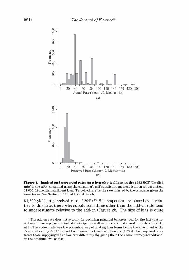
Payment/interest bias is the difference between the perceived and impliedAPRs. Figure 2a presents a histogram of payment/interest bias in the 1983SCF. Over 98% of respondents underestimate the actual rate. Roughly 20%of respondents give the “simple” or “add-on” rate (e.g., a repayment total of

16 The survey respondent is whomever was determined to be the “most knowledgeable aboutfamily finances.” We use the terms “household,” “individual,” “consumer,” and “borrower” inter-changeably.

17 See equation (4) for a formal definition of the APR. Although the SCF question does not specifya particular definition of “rate of interest,” we use the APR as our benchmark because: (1) it hasbeen the standard unit of comparison for borrowing costs in the United States since the enactmentof the Truth-in-Lending law in 1968; and (2) it is the rate respondents supply when asked about themost prevalent type of loan, home mortgages. Using alternative benchmarks such as the EffectiveAnnual Rate, which is higher than the APR and may be a better measure of true borrowing costs,does not change the results because we use cross-sectional variation in perceptions; that is, we userelative and not absolute bias (see equation (8)).

18 We assume that the monthly installment payments are equal when calculating the impliedAPR. Different assumptions about payment arrangements do not change the qualitative resultsthat respondents generally underestimate interest rates (even if we assume that the first 11 pay-ments are zero, and the last completely repays the loan). More importantly, while such transfor-mations change the level measure of misperception they do not alter the cross-sectional rankingin misperception. As noted directly above, it is this ranking that provides identification in ourempirical tests below.


020

040

060

080

010

00Fr

eque

ncy

0 20 40 60 80 100 120 140 160 180 200Actual Rate (Mean=57, Median=43)

(a)

(b)

050

010

0015

00Fr

eque

ncy

0 20 40 60 80 100 120 140 160 180 200Perceived Rate (Mean=17, Median=18)

Figure 1. Implied and perceived rates on a hypothetical loan in the 1983 SCF. “Impliedrate” is the APR calculated using the consumer’s self-supplied repayment total on a hypothetical$1,000, 12-month installment loan. “Perceived rate” is the rate inferred by the consumer given thesame terms. See Section I.C for additional details.

$1,200 yields a perceived rate of 20%).19 But responses are biased even rela-tive to this rate; those who supply something other than the add-on rate tendto underestimate relative to the add-on (Figure 2b). The size of bias is quite

19 The add-on rate does not account for declining principal balances (i.e., for the fact that in-stallment loan repayments include principal as well as interest), and therefore understates theAPR. The add-on rate was the prevailing way of quoting loan terms before the enactment of theTruth-in-Lending Act (National Commission on Consumer Finance (1972)). Our empirical worktreats those supplying the add-on rate differently (by giving them their own intercept) conditionalon the absolute level of bias.


020

040

060

0Fr

eque

ncy

-200 -160 -120 -80 -40 0 40 80 120 160 200Bias Relative to APR, (Mean=-38, Median=-25)

(a)

020

040

060

080

0Fr

eque

ncy

-200 -160 -120 -80 -40 0 40 80 120 160 200Bias Relative to Add-on, (Mean=-18, Median=-8)

(b)

Figure 2. Payment/interest bias. Figure 2a shows the distribution of payment/interest bias(the difference between the perceived and implied APRs on the hypothetical loan) across 1983 SCFhouseholds. Figure 2b measures bias as the difference between the perceived and add-on rates.The add-on rate divides total interest per year by the loan principal: It does not account for thedeclining principal balance.

striking, although not integral to our empirical work (which focuses on cross-sectional differences in bias). The median bias is −25 percentage points (2,500basis points), and the mean bias is −38 percentage points.20 Table I shows tab-ular data on payment/interest bias in both the 1983 and 1977 SCFs. The data

20 The Juster and Shay (1964) results allow one to infer something about the size of pay-ment/interest bias. Average bias in their sample of Consumers Union members is substantial(1,500 basis points) but smaller than in our samples.


Table IPayment/Interest Bias on Hypothetical Loans in the 1983 and 1977

Surveys of Consumer FinancesEach sample includes all households in the SCF for that year. Rates and bias are in hundreds ofbasis points. Payment, APR, and bias measures are means by quintile. Quintiles are by bias relativeto APR. “n/a” includes households that fail to supply either a repayment total or a perceived APR,or report neither. Observations per quintile differ due to clustered values of bias.

Bias Quintile, 1983 Data

1 2 3 4 5 n/a

Stated repayment total (P + I) 1,135 1,200 1,255 1,398 1,772 1,492Implied APR 24 35 44 66 114 76Perceived APR 16 18 17 18 15 16Payment/interest bias = −8 −16 −27 −48 −99 –

Perceived APR − Implied APRShare supplying add-on rate 0.58 0.42 0.09 0.02 0 –Range of bias in quintile [100, −14] [−14, −20] [−20, −33] [−33, −63] [−63, −290] –Number of households 698 713 662 729 612 689

Bias Quintile, 1977 Data

1 2 3 4 5 n/a

Stated repayment total (P + I) 1,107 1,177 1,211 1,284 1,542 1,362Implied APR 19 31 37 48 87 59Perceived APR 13 16 15 14 15 15Payment/interest bias = −6 −15 −22 −34 −73 –

Perceived APR − Implied APRShare supplying add-on rate 0.55 0.46 0.08 0.03 0.00 –Range of bias in quintile [5, −10] [−11, −17] [−18, −25] [−26, −42] [−43, −255] –Number of households 202 275 214 173 173 68

show that bias is similar in both surveys, although it is slightly smaller in the1977 data. We stratify bias into the quintiles that we use to measure relativedifferences in bias for our analysis of whether bias affects decisions.

While we do not know of any more recent representative data measuringpayment/interest bias, there is one bit of corroborating contemporary evidence.Following an internal presentation of this paper, a skeptical colleague gave anupdated version of the SCF questions to students in a finance class that hadrecently covered discounting. Of 37 students, all underestimated the APR: Onegave a rate above the add-on rate, 12 gave the add-on rate, and the remainderunderestimated relative to both the APR and the add-on rate.

C. New Evidence: Bias on Actual Loans

Both the 1983 and 1977 SCFs also contain self-reported interest rates onactual loans: on all installment loans in the 1977 SCF and on mortgages in the


Table IIPayment/Interest Bias on Actual Loans, by Maturity

and Hypothetical Loan Bias“Implied APR” is calculated from loan payment, maturity, and principal. “Perceived APR” is sup-plied by loan holder. Bias is (Perceived APR – Implied APR). Each cell presents a sample mean.Installment loan data are from 1977 SCF. Mortgage data are from 1983 SCF; implied mortgageAPRs are difficult to calculate in 1977 with any precision because the survey does not specifywhether escrow payments (for taxes and insurance) are included in the households monthly pay-ment. Mortgage maturity ranges from 120 to 360 months. “Low” and “High” bias are quintiles 1 to3 and 4 to 5 in Table I, respectively.

Installment Loans: Maturity (Months)

[0, 24] [25, 36] [37, 48] [49, 120] Mortgage Loans

All loan holdersImplied APR 30 28 22 17 9.8Perceived APR 13 12 12 12 9.2Payment/interest bias −15 −15 −8 −3 −0.6

Low hypothetical loan biasImplied APR 26 27 21 17 9.4Perceived APR 12 12 11 11 9.0Payment/interest bias −13 −14 −9 −5 −0.3

High hypothetical loan biasImplied APR 35 29 23 18 10.3Perceived APR 13 13 13 12 9.5Payment/interest bias −19 −17 −7 −1 −0.8

1983 SCF. This is useful because with self-reported data on principal, maturity,and payments, we can calculate the implied APR on each loan, assuming thatconsumers report non-interest loan terms accurately. This allows us to askwhether consumers also display payment/interest bias on actual loans, andmoreover whether payment/interest bias varies with loan maturity (recall thatthe hypothetical question concerns only a 1-year maturity).

Table II presents summary data on payment/interest bias on all actual non-mortgage installment loans in the 1977 SCF and all actual mortgages in the1983 SCF.21 The data reveal substantial payment/interest bias on short-termloans; for the shortest-maturity loans actual rates average 30% while perceivedrates average 13%. Payment interest bias on actual loans is positively corre-lated with payment/interest bias on hypothetical loans. This is evident fromthe bottom two panels of Table II.

The other striking result is that bias falls with maturity, and is close tozero for the longest-maturity installment loans and mortgage loans (which

21 We discard installment loan responses from 1977 that imply negative interest rates; in alllikelihood these are loans with balloon payments, which are not recorded. We also discard mortgagesfrom 1977, because that survey does not identify the size of escrow payments for taxes and insurancein each household’s mortgage payment, making calculation of the implied APR impossible.


themselves tend to have 15- to 30-year maturities). Virtually everyone is unbi-ased on mortgage loans; 96% provide the correct APR.

D. Summary of the Evidence on Payment/Interest and Future Value Bias

There are three sets of stylized facts on how consumers intuitively perceivethe costs and benefits of intertemporal tradeoffs. First, consumers systemati-cally display future value bias in the lab. Second, they systematically displaypayment/interest bias on both hypothetical and actual loans. Third, the severityof each bias depends on the time horizon. Future value bias is more severe forlong-term savings, while payment/interest bias is more severe on short-termloans.

When looking at these facts it is not surprising to see that consumers makemistakes, or even that they make large mistakes. The math of interest ratesand future values is complex (as detailed in the next section). The strikingthing is that consumers give answers that are biased: They almost alwaysunderestimate future values, and almost always underestimate loan interestrates. We now ask whether a common cognitive underpinning can explain notonly payment/interest bias and future value bias, but also the relationshipbetween each bias and the time horizon being considered.

II. Explaining Payment/Interest and Future Value Biases:Exponential Growth Bias and Other Possibilities

Here we consider several explanations for the pattern of payment/interestand future value bias documented above. In particular, we show that expo-nential growth bias (“EG bias”) provides a parsimonious explanation. EG biasis the tendency of individuals to systematically and dramatically underesti-mate the growth or decline of exponential series when asked to make intuitiveassessments (without calculators).22 Thirty years of research in cognitive psy-chology establishes that EG bias appears robustly across elicitation methodsand contexts (see Internet Appendix A for a review).

A. Exponential Growth Bias and Future Value Bias

It is intuitive that someone who underestimates exponential growth will dis-play future value bias. Consider a consumer who saves a present value (PV) ata periodic interest rate i over time horizon t, with periodic compounding. Thefuture value (FV) is

F V = PV (1 + i)t . (1)

22 We focus on exponentiation rather than on the other mathematical operations involved inborrowing and savings calculations because there is little evidence of biases in basic arithmetic.For reviews of related evidence see Campbell and Xue (2001) and DeStefano and LeFevre (2004).


The term f (i, t) = (1 + i)t is an exponential function, and an individual withEG bias will underestimate (1 + i)t. Because the future value is just a multipleof that term, there is a straightforward link between EG bias and future valuebias. Even a mild degree of EG bias can lead to substantial future value bias;consider a consumer with the following form of EG bias:

f (i, t, θ ) = (1 + i)(1−θ )t . (2)

The θ term parameterizes bias: Unbiased consumers have θ = 0 and cor-rectly perceive exponential growth, while those with 0 < θ < 1 have EG bias.23

Figure 3 shows how an EG-biased consumer would perceive future values overdifferent time horizons t = [1, 5, 30], with bias on the interval θ ∈ [0, 0.15].24

Figure 3 uses i = 7%, a benchmark return on equities. Perceived future valuesare calculated using

F V = PV · f (i, t, θ ). (3)

The calculations use annual compounding and PVs that equalize the FVwhen θ = 0, to facilitate comparison of perceived FVs as EG bias changes. Fig-ure 3 illustrates that EG bias is essentially irrelevant over a 1-year horizon,and has large effects over a retirement planning (30-year) horizon. We showthe effects for a single interest rate to conserve space, but it is evident from (1)and (2) that the level effects of bias are increasing in the interest rate.

Another parameterization of EG bias is “linear bias,” which is a useful bench-mark because it describes a complete failure to account for compounding. Themathematical form for linear bias is f (i, t) = 1 + it, meaning that the perceivedfuture value is linear in t. In lab experiments measuring EG bias, perceived fu-ture values are often closer to those implied by linear bias than to the truevalue.

B. Exponential Growth Bias and Payment/Interest Bias

Interest rate formulas also contain exponential functions. The formula re-lating a periodic interest rate i to a loan amount L, maturity t, and periodicpayment m is

m = Li + Li(1 + i)t − 1

. (4)

23 Most research in psychology estimating EG bias uses this functional form, because it fitsexperimental data reasonably well using only one free parameter. See Internet Appendix A for adiscussion of more flexible approaches.

24 This range of parameterized EG bias is actually small relative to that estimated by Eisen-stein and Hoch (2005) for savings. Eisenstein and Hoch fit the slightly more flexible functionf (i, t, α, β) = α(1 + i)βt and estimate (α ≅ 0.45, β ≅ 0.50). We use smaller values for EG bias be-cause they fit our loan data better. The median θ implied by the hypothetical loan questions usedin Figures 1a and 1b is 0.2, and the interquartile range is [0.14, 0.33]. The values implied by theactual loan questions from 1977 are smaller on average.


0

5000

10000

15000

20000

25000

0 0.01 0.02 0.03 0.04 0.05 0.06 0.07 0.08 0.09 0.1 0.11 0.12 0.13 0.14 0.15

Exponential Growth Bias (Theta)

Actual FV

Perceived FV, 1 year

Perceived FV, 5 years

Perceived FV, 30 years

Figure 3. Perceptions of future values with exponential growth bias. This numericalexample shows how exponential growth bias (“EG bias”) affects perceptions of future values receivedover different time horizons. All calculations use an annual interest rate of 7%. Future values arecalculated using:

F V = PV · f (i, t, θ ).

Actual FV uses an unbiased assessment of exponential growth:

f (i, t, 0) = (1 + i)t .

Perceived FV uses the parameterized function:

f (i, t) = (1 + i)(1−θ )t .

Higher θ indicates greater EG bias. This range of parameterized EG bias is actually small relativeto that estimated by Eisenstein and Hoch (2005) for savings. We use smaller values for EG biasbecause they fit the range of payment/interest bias in our data. For the 30-year time horizon, PV =$1,000. For the 5-year time horizon, PV = $5,427.50. For the 1-year time horizon, PV = $7,114.50.The three PVs equalize the FV when θ = 0, to facilitate comparison of perceived FVs as exponentialgrowth bias changes.

This equality contains the same exponential term that appears in the fu-ture value formula: f (i, t) = (1 + i)t .25 There is no closed-form solution for the

25 There are many ways to write the formula in (4); we choose this one to make the link betweenthe saving and borrowing calculations as clear as possible.


periodic rate; it is defined implicitly. If the period is 1 month, the annual per-centage rate (APR) on the loan is equal to 12i.26

Although the math is considerably more difficult than for future values, onecan also show that EG bias produces payment/interest bias.27 Internet Ap-pendix B presents a formal treatment of the issue, proving that EG bias pro-duces payment/interest bias and showing conditions under which bias is greaterfor short-term loans.

Despite the subtlety of the math involved, the intuition for this result isstraightforward. Payment/interest bias is a consequence of failing to accountfor declining principal balances on installment loans. The most common incor-rect answer on the hypothetical questions in Section I.C is the add-on interestrate, which represents the true cost of borrowing only if the borrower retains theloan principal for the entire loan term. But installment loans require borrowersto start repaying principal immediately, so given a fixed dollar amount of in-terest, the true cost of borrowing always exceeds the add-on rate.28 A consumerwho does not think about declining principal balances or underestimates theirimpact on borrowing costs will have the payment/interest bias we document inSections I.B and I.C.

The mathematical correspondence between EG bias and failing to account fordeclining principal balances is best illustrated by the linear bias case. Supposethat, instead of using the correct formula in (4) to infer the interest rate, aborrower with linear bias uses f (i, t) = 1 + it to solve for the interest rate:

m = Li + Li(1 + it) − 1

. (5)

In that case the closed-form solution for the periodic rate is exactly the simpleinterest rate on the loan:29

i = mt − LLt

. (6)

Thus, having a form of EG bias that completely fails to account for compound-ing is mathematically equivalent to the intuitive effect of completely failing toaccount for declining principal balances.

26 The APR is not continuously compounded. The continuously compounded rate, (1 + i)t, isknown as the Effective Annual Rate (EAR). It is not a widely used measure of borrowing costs.

27 In the next section, we discuss whether this accurately describes the inferences consumersactually make (or whether, for example, Truth-in-Lending, forcing lenders to disclose APRs, renderssuch inference unnecessary). Here our focus is simply on asking whether EG bias can explainpayment/interest bias in the context of the questions in Section I.

28 An alternative view of the intuition is that it reduces the effective loan principal on a short-term loan from L to something closer to L/2. That approximation generates a rule-of-thumb forshort-term installment loan APRs, which is that they are roughly double the add-on rate. Only 1%of our sample supplies a perceived APR that is consistent with the use of this heuristic.

29 Recall that this formula is for the periodic rate, and that the APR on a t-month loan is it. So,for a 12-month loan of $1,000 with monthly payments of $100 and total payments of $1,200 overthe year, the formula yields a periodic rate of 1.67%, and a (misperceived) APR of 12 × 1.67% =20%, which is the simple interest rate.


EG bias can also produce the (perhaps less intuitive) result that pay-ment/interest bias is more severe on short-term loans. This comes from the factthat principal balances decline less quickly as maturity increases. Consider thelimiting case. As the maturity on the loan approaches infinity, the last term inequation (4) disappears and the formula becomes m = Li; the periodic paymentequals the principal times the periodic rate. Because the exponential term dis-appears, even someone with severe EG bias will correctly infer the rate from aprincipal and payment. Put another way, on an infinite maturity (interest-only)loan, there is no declining principal balance to complicate inference about theinterest rate.30

Numerical examples also illustrate these ideas, and show that even mild EGbias generates substantial payment/interest bias. Figure 4 compares the actualto perceived interest rates on 12-, 48-, and 360-month installment loans, wheret = [12, 48, 360] and θ ∈ [0, 0.15]. All calculations use an actual APR of 35% (tofit the modal rate implied by the questions we use to measure bias) and thesame functional form for EG bias as in Figure 3, meaning that the perceivedrate solves31

m = Li + Li(1 + i)(1−θ )t − 1

. (7)

Even relatively low levels of EG bias (i.e., of θ ) lead to substantially lowerperceived interest rates and to payment/interest bias that is greater on theshort-term loans. It is essentially irrelevant on the 30-year loan.

A final point to highlight is that EG bias can produce biased perceptions ofborrowing cost and saving returns either directly or indirectly. The effect isdirect if consumers actually try to (intuitively) solve the problems describedabove. The effect is indirect if EG bias leads consumers to adopt biased heuris-tics like linearizing yields or ignoring declining principal balances.

C. Other Explanations for Payment/Interest Biasand the Bias/Maturity Pattern

EG bias is an appealing explanation for the biases documented in Section Ibecause it provides a simple and coherent explanation for the entire pattern

30 There is a limiting argument in the other direction as well, though it is looser. Suppose aconsumer underestimates the exponential term in the denominator of equation (4). As maturityt falls the denominator approaches zero, increasing the value of the second term and requiring alower perceived rate to make the equality hold (given a fixed loan principal and monthly payment).The statement is a bit imprecise because i itself appears in the exponential growth term, whichmotivates the more careful analysis in Internet Appendix B, but the general thrust of the argumentturns out to be correct.

31 The functional form in our numerical examples has the advantage of simplicity, but can yieldperceived rates that are zero or even negative if θ is large enough given the other parameters.We view that functional form as a useful approximation within the range of data that we observe,rather than a form that accurately models the effects of EG bias across a wide range of settings.Reassuringly, Internet Appendix B shows that EG bias generates payment/interest bias under verygeneral conditions on the form of bias.


0%

5%

10%

15%

20%

25%

30%

35%

40%

0 0.01 0.02 0.03 0.04 0.05 0.06 0.07 0.08 0.09 0.1 0.11 0.12 0.13 0.14 0.15

Exponential Growth Bias (Theta)

Actual APR

Perceived rate, 12 mo.

Perceived rate, 48 mo.

Perceived Rate, 360 mo.

Figure 4. Perceptions of borrowing interest rates with exponential growth bias. Thisnumerical example shows how exponential growth bias generates payment/interest bias. Weuse an actual APR of 35% (to match the modal APR implied by the repayment total re-sponses to the 1983 SCF hypothetical), and a loan principal of $1,000. Monthly paymentsare $100 on a 12-month loan, $38.85 on a 48-month loan, and $29.00 on a 360-month loan.

Implied and perceived rates solve the installment loan payment formula:

m = Li + Li[ f (i, t, θ ) − 1]

.

Actual APR uses an unbiased assessment of exponential growth:

f (i, t, 0) = (1 + i)t .

Perceived APR uses the parameterized function from Figure 3:

f (i, t) = (1 + i)(1−θ )t .

of biases. It also has broad experimental support in other settings. But it ispossible that there are other reasons for either the existence of payment/interestbias or the bias/maturity relationship. We now discuss those other explanations,noting which can be dismissed and which cannot.

One set of explanations is for the existence of payment/interest bias (or futurevalue bias) overall. At first blush one might think that payment/interest biassimply reflects math mistakes or uninformed guesses. It is certainly true thatcalculating an APR (or a future value) from other information is extremelydifficult, and the fact that people make mistakes is unsurprising. What issurprising is that when people make mistakes, they err in a particular direction.


Most evidence suggests that even on difficult questions the “wisdom of crowds”centers the distribution of answers on the truth (Surowiecki (2005)). Our find-ings suggest that something systematic moves the distribution of answers awayfrom the truth.

Another version of this explanation is that something mechanical about thesurvey questions leads people to supply perceived rates below actual rates. Butbias is evident on actual as well as hypothetical loans, and is robust to differentframes. Moreover, a framing effect would imply that bias is spurious and shouldbe uncorrelated with real-world outcomes; we test and reject that hypothesisbelow.

A more subtle mechanical influence might work through time-varying mar-ket rates. Say the SCF hypothetical elicits current market repayment totals(on average at least) and respondent perceptions of “normal” (rather than cur-rent) market rates. Then our measure will mechanically produce greater levelsof “bias” during a period when there are high market rates, as was the casein 1983. But this will only induce an empirical relationship between bias andhousehold finance if the propensity to mismatch current and normal rates iscorrelated with something else that drives decisions. If, on the other hand, thepropensity to mismatch rates is uncorrelated with financial decisions, then weshould see no relationship between what we call payment/interest bias and anyoutcome of interest.

In any case the perception data from 1977 belie this concern, because dur-ing that period rates were both stable and typical by historical standards.32

Table II shows that hypothetical loan bias is not much different in 1977from 1983. Moreover, bias is also prevalent on actual short-term loans in1977.

A second set of alternative explanations concerns the bias/maturity relation-ship. In this case there are plausible, complementary explanations for one fact:that consumers correctly assess the interest rates on their long-term loans. Onesuch explanation is that consumers learn and remember their mortgage ratesbecause the stakes are high. Another explanation is that enforcement of theAPR disclosure, mandated by the Truth-in-Lending Act (TILA), is effective formortgages. Indeed, our related work provides evidence consistent with this hy-pothesis; TILA has more bite for banks than nonbanks, and banks dominatedthe mortgage market during our sample period. So, both of these factors couldexplain why consumers have accurate (and precise) knowledge of interest rateson long-term loans. Neither explains payment/interest bias on short-term loans,however.

In sum, EG bias or one of its intuitive analogues provides a coherent explana-tion for the pattern of misperceptions documented in Section I. No alternativeexplanation that we know of explains the entire pattern. We consider the pos-sibility that our measure of bias is correlated with other factors that drivefinancial decisions in Section V.

32 The 10-year T-bill rate was 7.21% on January 1, 1977. It averaged 7.24% and 6.71% duringthe previous 5- and 10-year periods.


D. Could Bias Matter in the Market?

A final issue of interpretation is whether payment/interest bias or futurevalue bias could matter in the market. As noted in the Introduction, there areseveral reasons to believe that bias might not be completely neutralized.

On the consumer side, the mitigating effects of learning, heuristics (includ-ing ignoring interest rates), and decision aids may be incomplete in a relativelyabstract, low-feedback domain like household finance. On the supply side, in-complete Truth-in-Lending enforcement may allow many lenders to continueexploiting bias by shrouding interest rates, and SEC rules discourage the typeof advertising that may be needed to debias consumers (namely, advertisingfeaturing expected future value earned over long investment horizons).

In the next two sections we detail our tests of the hypothesis that bias isneutralized or otherwise irrelevant in the market. We also test whether supply-or demand-side forces such as delegation and credit constraints counteract theeffects of bias.

III. Exponential Growth Bias and Household Finance:Empirical Strategy

We outline our empirical strategy in this section, and then detail our testsand report the main results in Section IV.

A. Payment/Interest Bias and Household Finance in the Cross-section

Our empirical models estimate whether household-level differences in biasexplain the cross-section of outcomes in household finance. We lack a household-level measure of future value bias, and therefore focus on our measure of pay-ment/interest bias as the key explanatory variable. We use specifications of theform:

Outcomeh = f (Biash, Addonh, X h). (8)

The dependent variable Outcome varies in each model; we discuss the out-come measures below. The vector Bias contains payment/interest bias quintileindicators and a separate category for nonresponse to the hypothetical loanquestions.33 The latter allows for the possibility that nonresponders are morebiased than the least-biased (i.e., quintile 1) households. The variable Addonis a dummy equal to one if the perceived rate (used in the payment/interestbias measure) equals the add-on rate; including this as a covariate allowsfor the possibility that households providing the add-on rate interpret the

33 We have used other functional forms for bias (a biased/unbiased indicator, the logarithm ofbias, and a quadratic in the level of bias). The results are robust to these other functional forms, aswell as to orthogonalizing bias by regressing ln(bias) on the full set of controls, and then using thedeviation of actual bias from its fitted value to reconstruct bias quintiles. See Internet AppendixTable IA.I for some results.


payment/interest bias questions and/or behave differently, conditional on thedegree of bias. The vector X contains all of the controls detailed below.

Intuitively, we would expect that payment/interest bias should increase short-term but not long-term borrowing, decrease savings rates, and decrease networth.34 If payment/interest bias is also a useful measure of future value bias(which would be true if both are driven by a common exponential growth bias),then Bias should be correlated with asset allocation as well as debt allocation,and exert stronger effects over the long term and for high-return assets. Wetherefore test whether bias decreases long-term (and high-yielding) but notshort-term (and low-yielding) investing.

The null hypothesis in each case is that the coefficients on Bias are zero (ei-ther because our bias measure is uninformative, or because bias is neutralizeddue to consumer or supplier adaptation). The least-biased households (quintile1) serve as the omitted category.

B. Data, Outcomes, and Control Variables

In the empirical work below we use data from the 1983 SCF rather thanthe 1977 SCF, because the 1983 survey covers the household balance sheetmore comprehensively. The top panel of Table III shows our outcome measures,stratified by bias category. We discuss the outcomes in greater detail below, butto summarize they are: short-term debt/income, long-term debt/income, stockholdings as a share of total assets, CD holdings as a share of total assets,savings rates, and wealth accumulation. Not surprisingly, there are strong un-conditional relationships between bias and all of the outcomes of interest. Thishighlights the need to control for other influences on household finance.

An advantage of the SCF is that the set of possible controls is extensive.Because minimizing omitted variable bias is critical, we take an approachthat seeks to control for all factors that might be correlated with both out-comes and our measure of payment/interest bias, hence erring on the sideof “over-controlling.”35 Our controls include measures of preferences, expecta-tions, available resources (including income, defined-benefit retirement wealth,and credit constraints), claims on resources (including life-cycle factors), andproblem-solving approaches (and financial sophistication more generally). Wegroup them below for expositional purposes but emphasize that each of ourempirical models includes all of the variables described below (and detailedcompletely in Internet Appendix C). Table III shows descriptive statistics onsome key variables by bias category. Table IV (discussed in Section III.C)estimates multivariate correlations between bias and the control variables.

34 There may be income or other effects as well, particularly if payment/interest bias is gener-ated by exponential growth bias; for example, EG bias may lead to lesser discounting of a givenexpected future income stream and thereby make consumers feel wealthier. In that case we viewour empirical work as identifying the net effect of biased perceptions on our outcomes.

35 If there is a causal link between bias and any of these variables, we may underestimate therelationship between bias and our outcomes of interest (Angrist and Krueger (1999)).


Tab

leII

IP

aym

ent/

Inte

rest

Bia

san

dH

ouse

hol

dC

har

acte

rist

ics:

Des

crip

tive

Sta

tist

ics

from

the

1983

SC

FT

he

SC

F’s

advi

cequ

esti

onas

kssp

ecif

ical

lyab

out

gett

ing

hel

pon

savi

ngs

and

inve

stm

ent

deci

sion

s.N

um

ber

ofob

serv

atio

ns

are

show

nfo

rbo

rrow

ing

mea

sure

sth

atar

eco

ndi

tion

alon

hav

ing

non

zero

debt

.Res

ult

sar

ere

port

edin

1983

doll

ars.

Bia

sQ

uin

tile

12

34

5n

/a

Fin

anci

alou

tcom

es(1

)F

inan

ced

larg

ere

cen

tpu

rch

ase

Mea

n0.

230.

300.

330.

370.

410.

31N

458

456

382

412

301

236

(2)

Sh

ort-

term

inst

allm

ent

debt

outs

tan

din

g/in

com

eM

ean

0.16

0.19

0.18

0.16

0.20

0.21

N25

431

827

134

027

317

9(3

)L

ong-

term

debt

outs

tan

din

g/in

com

eM

ean

0.89

0.86

1.12

0.79

0.81

0.78

N48

353

845

049

934

725

1(4

)S

tock

shar

eof

asse

ts0.

120.

090.

050.

040.

020.

03(5

)S

tock

shar

eof

fin

anci

alas

sets

0.20

0.15

0.10

0.08

0.04

0.05

(6)

Dis

save

dla

stye

ar0.

280.

390.

450.

440.

430.

37(7

)T

otal

asse

ts(0

00s)

Med

ian

$90

$74

$41

$39

$31

$19

(8)

Tot

alde

bt(0

00s)

Med

ian

$7$1

2$5

$5$2

$0(9

)N

etw

orth

(000

s)M

edia

n$9

3$7

5$4

0$3

5$2

7$1

9D

emog

raph

ics

(10)

Did

not

fin

ish

hig

hsc

hoo

l0.

080.

040.

080.

100.

170.

36(1

1)S

ome

hig

hsc

hoo

l0.

070.

070.

120.

140.

160.

19(1

2)F

inis

hed

hig

hsc

hoo

l0.

230.

260.

340.

320.

340.

26(1

3)S

ome

coll

ege

0.19

0.23

0.22

0.22

0.17

0.11

(14)

Fin

ish

edco

lleg

e0.

430.

400.

240.

210.

160.

09(1

5)A

geM

ean

5046

4544

4656

(16)

Mal

eh

ead

0.88

0.86

0.81

0.78

0.69

0.56

(17)

Wh

ite

0.90

0.91

0.87

0.83

0.83

0.72

(18)

Lab

orin

com

e($

1,98

3)M

ean

$53,

973

$37,

209

$22,

229

$23,

459

$16,

189

$9,3

16S

D(1

18,8

15)

(68,

841)

(46,

566)

(48,

452)

(23,

078)

(22,

953)

Med

ian

$18,

995

$20,

000

$15,

000

$16,

257

$12,

000

$0

(con

tin

ued

)


Tab

leII

I—C

onti

nu

ed

Bia

sQ

uin

tile

12

34

5n

/a

Bor

row

ing

con

stra

ints

(19)

Den

ied/

disc

oura

ged/

rati

oned

0.12

0.15

0.16

0.19

0.20

0.15

(20)

Has

acr

edit

card

0.81

0.82

0.70

0.65

0.55

0.39

Pre

fere

nce

sR

isk (21)

Tak

essu

bsta

nti

alfi

nan

cial

risk

s0.

100.

050.

060.

080.

060.

04(2

2)T

akes

>av

erag

efi

nan

cial

risk

s0.

210.

170.

140.

130.

100.

06(2

3)T

akes

aver

age

fin

anci

alri

sks

0.39

0.48

0.43

0.40

0.34

0.24

(24)

Not

wil

lin

gto

take

any

fin

anci

alri

sks

0.30

0.30

0.37

0.39

0.50

0.65

Deb

tav

ersi

on(2

5)T

hin

ksbu

yin

gon

cred

itis

good

idea

0.46

0.50

0.47

0.47

0.44

0.36

(26)

Th

inks

buyi

ng

oncr

edit

isgo

odan

dba

d0.

320.

310.

320.

310.

310.

28(2

7)T

hin

ksbu

yin

gon

cred

itis

bad

idea

0.22

0.19

0.20

0.22

0.25

0.32

Pat

ien

ce/

liqu

idit

y(2

8)W

illt

ieu

pm

oney

lon

g-ru

nto

earn

subs

tan

tial

retu

rns

0.16

0.17

0.12

0.15

0.11

0.09

(29)

Wil

ltie

up

mon

eym

ediu

m-r

un

toea

rn>

aver

age

retu

rns

0.39

0.34

0.29

0.28

0.24

0.13

(30)

Wil

ltie

up

mon

eysh

ort-

run

toea

rnav

erag

ere

turn

s0.

260.

300.

330.

330.

290.

24(3

1)W

illn

otti

eu

pm

oney

atal

l0.

180.

170.

230.

250.

360.

46F

inan

cial

advi

ce(3

2)U

ses

any

fin

anci

alad

vice

0.50

0.57

0.56

0.58

0.52

0.43

(33)

Use

spr

ofes

sion

alfi

nan

cial

advi

ce0.

320.

370.

310.

290.

280.

21(3

4)U

ses

advi

cefr

omfr

ien

ds/f

amil

y0.

250.

310.

310.

370.

330.

26(3

5)U

ses

advi

cefr

omfr

ien

ds/f

amil

yon

ly0.

160.

190.

230.

270.

240.

21N

um

ber

ofob

serv

atio

ns,

un

con

diti

onal

outc

omes

698

713

662

729

612

689


Table IVPayment/Interest Bias and Household Characteristics: Multivariate

CorrelationsThis table presents results for the full sample except for those with unknown bias (or negative biasin columns 3 and 4). Huber–White standard errors are shown in parentheses. OLS regressionsof payment/interest bias quintile (or the natural logarithm of (− bias)) on the RHS variables arelisted in the row headings. Columns 2 and 4 also include the full set of covariates in addition tothose reported in the table: marital status, household size, employment status, health, homeowner-ship, industry, occupation (including self-employment), pension coverage, Social Security + pensionwealth decile, years in current job, any expected inheritance, expected retirement age, expectedtenure at current job, use of advice on saving and investment decisions, ATM use, comparing loanterms on price vs. non-price margins, denied/discouraged/turned down for credit, and credit cardholding.

Bias Quintile ln(Bias)

LHS Variable: (1) (2) (3) (4)

Wage income quintile 2 −0.014 −0.150 −0.000 −0.063(0.088) (0.095) (0.055) (0.060)

Wage income quintile 3 0.127∗ 0.038 0.071 0.026(0.077) (0.087) (0.047) (0.052)

Wage income quintile 4 0.054 −0.027 0.024 −0.023(0.077) (0.092) (0.046) (0.055)

Wage income quintile 5 −0.200∗∗∗ −0.238∗∗ −0.098∗∗ −0.148∗∗(0.075) (0.094) (0.047) (0.058)

Some high school −0.174 −0.101 −0.092 −0.052(0.108) (0.112) (0.066) (0.070)

Finished high school −0.426∗∗∗ −0.265∗∗ −0.263∗∗∗ −0.179∗∗∗(0.099) (0.107) (0.061) (0.067)

Some college −0.634∗∗∗ −0.397∗∗∗ −0.366∗∗∗ −0.240∗∗∗(0.104) (0.117) (0.064) (0.072)

Finished college −0.847∗∗∗ −0.535∗∗∗ −0.462∗∗∗ −0.292∗∗∗(0.102) (0.125) (0.064) (0.078)

Age −0.013 −0.006 −0.008 −0.008(0.009) (0.013) (0.006) (0.008)

Age squared 0.000 0.000 0.000 0.000(0.000) (0.000) (0.000) (0.000)

Male −0.332∗∗∗ −0.358∗∗∗ −0.204∗∗∗ −0.225∗∗∗(0.063) (0.095) (0.037) (0.056)

Black 0.203∗∗ 0.151∗ 0.142∗∗∗ 0.107∗∗(0.080) (0.086) (0.051) (0.054)

Hispanic −0.028 −0.083 0.102 0.048(0.144) (0.146) (0.092) (0.094)

Other nonwhite −0.332 −0.409∗ −0.195 −0.240∗(0.236) (0.240) (0.133) (0.135)

Take > average financialrisks expecting to earn >

average returns

0.036 0.045 0.047 0.049

(omitted = takesubstantial risksexpecting to earnsubstantial returns)

(0.105) (0.103) (0.070) (0.070)

Take average financial risks 0.045 0.042 0.068 0.068expecting to earn average (0.093) (0.092) (0.063) (0.062)returns

(continued)


Table IV—Continued

Bias Quintile ln(Bias)

LHS Variable: (1) (2) (3) (4)

Not willing to take any 0.126 0.083 0.116∗ 0.095financial risks (0.097) (0.097) (0.065) (0.064)

Thinks buying on credit isgood and bad

0.023 0.016 0.037 0.034

(omitted = thinks buyingon credit is good idea)

(0.053) (0.053) (0.032) (0.033)

Thinks buying on credit is 0.052 0.002 0.035 0.007bad idea (0.061) (0.062) (0.038) (0.039)

Will tie up moneymedium-run to earn >

average returns

−0.068 −0.060 −0.067 −0.065

(omitted = will tie upmoney long-run to earnsubstantial returns)

(0.073) (0.072) (0.045) (0.044)

Will tie up money short-run −0.004 0.014 −0.038 −0.020to earn average returns (0.074) (0.074) (0.046) (0.045)

Will not tie up money at all 0.136 0.123 0.056 0.052(0.084) (0.085) (0.053) (0.053)

Full set of controls? No Yes No YesR2 0.13 0.17 0.12 0.15N 3,414 3,414 3,313 3,313

∗, ∗∗, ∗∗∗ indicate 10%, 5%, and 1% level of significance, respectively.

Controls for available resources and claims on resources include: total house-hold labor income (dummies for the percentile), homeownership, pension cov-erage, pension wealth and Social Security wealth (we exclude this wealth fromour left-hand-side wealth measure since it was plausibly beyond the direct con-trol of most households in 1983), number of members in the household, gender,education, race, age, marital status, health status, years with current employer,industry, and occupation (including business ownership or self-employment ac-tivity). We also observe two measures of credit constraints: whether a householdhas been denied credit or discouraged from applying in the “past few years,”and whether the household has a credit card.

Controls for expectations about life-time wealth include measures of expectedinheritance, expected tenure with current employer, and expected retirementage.

Controls for preferences include measures of risk preference, liquidity pref-erence, and debt aversion; other work has shown that these are important de-terminants of household financial decisions. Risk preference is measured withthe question: “Which of the following statements on this card comes closest tothe amount of financial risk you are willing to take when you save or makeinvestments?” Answers fall into four categories, ranging from “willing to takesubstantial financial risks to earn substantial returns” to “not willing to take


any financial risks.” Time preference or patience is measured with the question:“Which of the following statements on this card comes closest to how you feelabout tying up your money in investments for long periods of time?” Answersrange from “will tie up money in the long run to earn substantial returns” to“will not tie up money at all.” Debt aversion (and perhaps an element of timepreference) is measured with the question: “Do you think it is a good idea ora bad idea for people to buy things on the installment plan?” We consider theimplications of possible omitted “behavioral” biases in preferences and expec-tations in Section V.B.

Controls for problem-solving approaches and overall financial sophisticationinclude whether the respondent evaluates loan offers by focusing on APRs orother terms (e.g., monthly payment, available loan amount, down payment,collateral requirement). Focusing on payments or other terms may reflect alack of financial sophistication, conditional on credit constraints.36 Two otherproxies for financial sophistication are ATM use (only 17% of our sample useATMs at all), and of course education. We consider the possibility that elementsof financial sophistication remain unmeasured, and the relationship betweenbias and financial sophistication more broadly, in Section V.A.

Controls for financial advice are categorical variables measuring whetherhouseholds use external advice, and whether advice is from a professional,from friends and family, or from other sources.

C. Who Is Biased? Multivariate Relationships

Table IV sheds light on the conditional relationships between household char-acteristics and bias by presenting results from models with a measure of biason the left-hand side and sets of controls on the right-hand side. We use twofunctional forms for bias: bias quintile and ln(−Bias); the latter coefficients areeasier to interpret but discard observations with zero or positive bias. For eachdependent variable, we present a parsimonious specification including a sub-set of important RHS variables, and a full specification with all of the controlslisted above. One difference between these specifications and those we use be-low is that we use wage income quintile as a control here; below we use wageincome percentile, which is much more flexible.

Not surprisingly, income and education are highly correlated with bias. Theserelationships hold up even conditional on all of our other controls. Gender andrace are correlated with bias as well. Our preference variables, somewhat sur-prisingly, are not correlated with bias once we control for income and education;we consider possible omitted features of preferences in Section VI.B.

A final point is that the fit is quite low. In the parsimonious specifications, 12%to 13% of the cross-sectional variation in bias is explained by other householdcharacteristics. Even in the full models, household characteristics explain only15% to 17% of the variation in bias. That is surprising given the sheer number

36 Focusing on non-interest terms may be rational for those who face binding liquidity con-straints; see Adams, Einav, and Levin (2009), Attanasio, Goldberg, and Kyriazidou (2008), andKarlan and Zinman (2008).


of controls and the highly flexible functional form for many of them (the totalnumber of categorical variables is over 200). Bias is not easily explained byother household characteristics.

IV. Results

This section reports results of our primary empirical tests from the multi-variate model (8). Each multivariate specification conditions on the full set ofcontrol variables listed in Section III.B; some contain additional controls notedbelow. The tables suppress most of the control variable coefficients (includingthose on wage income percentile) to save space.

A. Liability Composition and Bias

Table V presents results of our test of whether payment/interest bias en-courages short-term borrowing (by making it appear relatively cheap) but notlong-term borrowing (since even individuals with severe payment/interest biasshould accurately assess long-term interest rates).

Column 1 presents probit marginal effects from a model where the depen-dent variable equals one if the household used short-term installment debt tofinance a recent large purchase (car, household item, or home improvement).37

This model also controls for characteristics of the recent purchase (month/year,product purchased, and product price). The coefficient on each of the bias quin-tiles is positive, and households in quintiles 4, 5, and the nonresponse categoryare significantly more likely than the least-biased households (in the omittedquintile 1) to have used short-term debt for the purchase. Each of the bias coef-ficients implies economically large increases (11% to 43% of the sample mean).Columns 2 and 3 test whether more-biased households have higher short-termdebt-to-income ratios, conditional on having nonzero short-term debt.38 Col-umn 2 includes the entire sample of short-term borrowers, while column 3drops households that face relatively severe credit constraints (measured byrecent credit denial or lack of a credit card). Overall, the results show a clearpositive relationship between short-term borrowing and bias: All of the 10 biascoefficients are positive. The results are stronger statistically when constrainedhouseholds are dropped from the sample, presumably because rationing pre-vents some households from borrowing as much as they would like. The pointestimates suggest that bias increases the short-term debt-to-income ratio from

37 This result is conditional on having made a large purchase; we find no significant relationshipbetween bias and the probability of purchase.

38 We find no relationship between bias and having nonzero short-term debt. It may be that theextensive margin is not very elastic—short-term installment debt is used primarily for financingvehicles and consumer durables, and the near absence of second mortgage markets in 1983, alongwith small credit card credit lines, implies that savings was the main outside option for these typesof purchase (responses to SCF question b5606, on the financing method for a large recent purchase,confirm this).


Table VShort-Term Debt, Long-Term Debt, and Payment/Interest Bias

Huber–White standard errors are shown in parentheses. Probit results are marginal effects. Allspecifications include controls for the full set of covariates in addition to the those reported inthe table: marital status, household size, employment status, health, homeownership, industry,occupation (including self-employment), pension coverage, Social Security + pension wealth decile,years in current job, any expected inheritance, expected retirement age, expected tenure at currentjob, use of advice on saving and investment decisions, ATM use, and comparing loan terms on pricevs. non-price margins. Columns 1, 2, and 4 include controls for denied/discouraged/turned downfor credit and for credit card holding. Column 1 includes controls for date, type, and amount ofpurchase.

Financed Last Short-Term Installment Long-TermBig Purchase? Debt/Income Debt/Income

(Probit) (OLS) (OLS)LHS Variable:Estimator: 0.32 0.18 0.17 0.88 0.82Mean(LHS): (1) (2) (3) (4) (5)

Bias quintile 2 0.036 0.043 0.066∗∗ −0.039 0.071(0.036) (0.027) (0.031) (0.105) (0.105)

Bias quintile 3 0.041 0.042 0.051∗ 0.215 0.008(0.042) (0.026) (0.028) (0.243) (0.126)

Bias quintile 4 0.079∗ 0.056∗∗ 0.065∗∗ −0.138 0.091(0.045) (0.026) (0.029) (0.160) (0.150)

Bias quintile 5 0.138∗∗∗ 0.055∗ 0.092∗∗∗ −0.166 0.046(0.051) (0.031) (0.034) (0.187) (0.140)

Bias unknown 0.100∗ 0.055 0.059 −0.255 −0.040(0.055) (0.038) (0.047) (0.214) (0.151)

Perceived rate = add-on 0.090∗∗ 0.062∗∗ 0.066∗∗ −0.121 −0.021(0.035) (0.025) (0.028) (0.123) (0.097)

Some high school 0.020 0.044 0.082 0.280 0.049(0.056) (0.038) (0.067) (0.188) (0.217)

Finished high school −0.027 0.010 0.047 0.564∗ 0.111(0.047) (0.031) (0.059) (0.326) (0.230)

Some college −0.043 0.037 0.052 0.565∗∗ 0.421(0.050) (0.036) (0.062) (0.225) (0.291)

Finished college −0.107∗∗ 0.026 0.050 0.450∗∗ 0.274(0.051) (0.039) (0.066) (0.216) (0.258)

Age 0.001 −0.005 −0.021∗∗ 0.086∗∗ 0.047∗(0.006) (0.005) (0.009) (0.042) (0.027)

Age squared −0.000 0.000 0.000∗∗ −0.001∗∗ −0.001∗∗(0.000) (0.000) (0.000) (0.000) (0.000)

Male 0.012 0.044 0.024 −0.391 −0.105(0.047) (0.036) (0.045) (0.274) (0.181)

Black 0.151∗∗∗ 0.012 0.028 −0.025 −0.061(0.050) (0.023) (0.033) (0.115) (0.112)

Hispanic −0.100∗ 0.032 0.035 0.234 0.005(0.054) (0.035) (0.048) (0.229) (0.190)

Other nonwhite −0.039 0.001 −0.123∗∗ 0.032 0.012(0.077) (0.061) (0.058) (0.261) (0.200)

Take > averagefinancial risksexpecting to earn >

average returns

0.084 −0.048 −0.049 −0.291 −0.432

(continued)


Table V—Continued

Financed Last Short-Term Installment Long-TermBig Purchase? Debt/Income Debt/Income

(Probit) (OLS) (OLS)LHS Variable:Estimator: 0.32 0.18 0.17 0.88 0.82Mean(LHS): (1) (2) (3) (4) (5)


(0.056) (0.039) (0.063) (0.222) (0.267)

Take average financial 0.094∗∗ −0.031 −0.058 −0.384∗ −0.632∗∗risks expecting to (0.046) (0.037) (0.057) (0.211) (0.270)earn average returns

Not willing to take any 0.083∗ −0.015 −0.019 −0.065 −0.512∗financial risks (0.050) (0.039) (0.056) (0.292) (0.266)

Thinks buying on creditis good and bad

−0.077∗∗∗ 0.006 0.003 0.155 0.061

(omitted = thinksbuying on credit isgood idea)

(0.022) (0.016) (0.018) (0.119) (0.082)

Thinks buying on credit −0.112∗∗∗ −0.003 −0.020 −0.020 −0.024is bad idea (0.023) (0.019) (0.022) (0.093) (0.098)

Will tie up moneymedium-run to earn> average returns

−0.025 −0.027 −0.017 0.208 0.113

(omitted = will tieup money long-runto earn substantialreturns)

(0.032) (0.026) (0.029) (0.156) (0.096)

Will tie up money 0.002 −0.000 0.011 −0.039 0.172short-run to earn (0.034) (0.028) (0.030) (0.150) (0.116)average returns

Will not tie up money 0.016 −0.039 −0.019 −0.205 0.154at all (0.039) (0.030) (0.033) (0.256) (0.154)

(Pseudo-) R2 0.32 0.17 0.24 0.11 0.17

Sample: Recent purchase Nonzero short-term debt Nonzero long-term debt

Dummies for wageincome percentile?

Yes Yes Yes Yes Yes

Exclude those denied,discouraged, orrationed in past fewyears?

No No Yes No Yes

Exclude those lacking acredit card?

No No Yes No Yes

Number of 2,221 1,635 1,011 2,568 1,869observations



23% to 54%. Households with a perceived rate that equals the add-on rate alsocarry significantly more short-term debt, conditional on the bias quintile.

Columns 4 and 5 show that payment/interest bias is not significantly cor-related with greater long-term debt (mostly mortgages and lines of credit).Here the long-term debt-to-income ratio is the outcome of interest. Notethat our usual set of control variables includes homeownership status.The sign pattern on the bias coefficients is less pronounced, and none of thebias quintile or add-on coefficients is significant, although the estimates areimprecise.

In sum, the evidence is consistent with exponential growth bias affectingborrowing choices via its effect on payment/interest bias.

B. Asset Composition and Bias

Table VI examines the relationship between payment/interest bias and thecomposition of assets. If payment/interest bias is confined to the borrowingside, then asset choices should be unaffected by bias. If, on the other hand,payment/interest bias is a useful proxy for future value bias, then it should benegatively related to holdings of long-horizon, high-yielding assets. We proxyfor long-term savings using the value of stock holdings (trading costs were highand mutual fund penetration was low in 1983), and for short-term savings usingthe value of CD holdings.39 For each outcome we measure holdings as a shareof total assets, and also as a share of financial assets (which exclude housingassets). These models condition on net worth decile in addition to our usual setof controls.

Columns 1 and 2 show that bias is negatively related to the proportion ofassets held in stocks. All of the bias coefficients are negative, and 8 out of10 are statistically significant. The coefficients imply that bias induces largedecreases in stockholding (of 18% to 55% of the sample means). The controlsalso enter the empirical relationship in meaningful ways. Higher education(shown in the table) and income (not shown because it is specified as a vector ofpercentile dummies) are both positively correlated with stock ownership. Ourmeasures of risk aversion and impatience are both negatively correlated withstock ownership.

Columns 3 and 4 report the same share specifications for CDs. The pattern ofsigns (all positive) and significance (6 out of 10) suggests that biased householdssubstitute short-term for long-term assets.

In sum, the results are consistent with exponential growth bias affectingasset composition via future value bias.

39 The presumption here is that stocks have a higher historical return, and are typically held overlonger time periods. There is a consensus that this is true; see Welch (2000, 2008) for discussions ofconsensus estimates of the equity premium. Of course, the early 1980s were a time of atypically highnominal interest rates, and, if people use nominal returns to allocate assets, that might weakenthe relationship between EG bias and stock or CD holdings.


Table VIStocks, CDs, and Payment/Interest Bias

We define stock ownership as holding any public equities or non-money market mutual funds. Only8% of the sample holds any mutual funds. Huber-White standard errors are shown in parentheses.All specifications include controls for the full set of covariates in addition to the those reportedin the table: marital status, household size, employment status, health, homeownership, industry,occupation (including self-employment), pension coverage, Social Security + pension wealth decile,years in current job, any expected inheritance, expected retirement age, expected tenure at currentjob, use of advice on saving and investment decisions, ATM use, comparing loan terms on price vs.non-price margins, denied/discouraged/turned down for credit, and credit card holding.

Stock Share of: CD Share of:

LHS Variable: Total Assets Fin. Assets Total Assets Fin. AssetsEstimator: (OLS) (OLS)

Mean(LHS): 0.06 0.10 0.04 0.09(1) (2) (3) (4)

Bias quintile 2 −0.011 −0.026∗∗ 0.008 0.021∗(0.009) (0.013) (0.007) (0.012)

Bias quintile 3 −0.019∗ −0.029∗∗ 0.013 0.029∗∗(0.010) (0.014) (0.008) (0.013)

Bias quintile 4 −0.018∗ −0.037∗∗∗ 0.014∗ 0.029∗∗(0.009) (0.014) (0.008) (0.013)

Bias quintile 5 −0.032∗∗∗ −0.055∗∗∗ 0.008 0.011(0.009) (0.013) (0.008) (0.014)

Bias unknown −0.012 −0.031∗∗ 0.018∗∗ 0.043∗∗∗(0.010) (0.014) (0.009) (0.015)

Perceived rate = add-on 0.006 −0.012 0.012∗ 0.018(0.008) (0.012) (0.007) (0.011)

Some high school 0.004 0.006 0.022∗∗ 0.035∗∗(0.006) (0.008) (0.009) (0.016)

Finished high school −0.001 0.011 0.021∗∗∗ 0.024(0.006) (0.009) (0.008) (0.015)

Some college −0.009 0.002 0.017∗ 0.018(0.008) (0.011) (0.009) (0.017)

Finished college 0.019∗ 0.047∗∗∗ 0.013 0.014(0.011) (0.015) (0.011) (0.019)

Age −0.005∗∗∗ −0.006∗∗∗ −0.002∗∗ −0.003∗(0.001) (0.002) (0.001) (0.002)

Age squared 0.000∗∗∗ 0.000∗∗∗ 0.000∗∗∗ 0.000∗∗(0.000) (0.000) (0.000) (0.000)

Male 0.000 −0.009 −0.010 −0.018(0.010) (0.012) (0.009) (0.014)

Black −0.009∗ −0.008 −0.017∗∗∗ −0.038∗∗∗(0.005) (0.008) (0.005) (0.008)

Hispanic −0.025∗∗∗ −0.028∗∗∗ −0.008 −0.021(0.006) (0.009) (0.010) (0.015)

Other nonwhite −0.027∗ −0.061∗∗ 0.025 0.039(0.016) (0.025) (0.021) (0.036)


average returns

0.017 0.012 0.009 −0.020

(continued)


Table VI—Continued

Stock Share of: CD Share of:

LHS Variable: Total Assets Fin. Assets Total Assets Fin. AssetsEstimator: (OLS) (OLS)

Mean(LHS): 0.06 0.10 0.04 0.09(1) (2) (3) (4)


(0.013) (0.017) (0.009) (0.016)

Take average financial risks −0.009 −0.023 0.011 −0.011expecting to earn average (0.011) (0.015) (0.007) (0.015)returns

Not willing to take any −0.017 −0.038∗∗∗ 0.019∗∗ 0.015financial risks (0.010) (0.014) (0.008) (0.016)


−0.004 −0.005 0.005 0.004


(0.005) (0.007) (0.005) (0.008)

Thinks buying on credit is 0.002 −0.006 0.008 0.012bad idea (0.006) (0.008) (0.006) (0.009)


average returns

−0.017∗∗ −0.014 0.002 0.017


(0.009) (0.012) (0.007) (0.012)

Will tie up money short-run −0.023∗∗∗ −0.026∗∗ −0.006 −0.004to earn average returns (0.009) (0.012) (0.007) (0.012)

Will not tie up money at all −0.016∗ −0.012 −0.043∗∗∗ −0.083∗∗∗(0.008) (0.012) (0.008) (0.013)

Dummies for wage incomepercentile?

Yes Yes Yes Yes

Dummies for net worthdecile?

Yes Yes Yes Yes

R2 0.37 0.35 0.17 0.21Number of observations 4,103 4,103 4,103 4,103


C. Saving, Wealth, and Bias

Table VII shows results for specifications correlating bias with savingsrates and wealth accumulation. For savings we estimate an ordered probit,where the categories are ranked (1: dissaved, 2: even, 3: saved) based on aquestion about household spending versus income in the previous year. Forwealth the dependent variable is the log of net worth.40 As with the borrowing

40 This drops the 7% of our sample with zero or negative wealth. We do not find any significantcorrelations between bias and having nonpositive wealth. We have also used net worth percentileas the dependent variable and obtain nearly identical results.


Table VIISaving, Net Worth, and Payment/Interest Bias

Huber-White standard errors are shown in parentheses. Sample sizes in columns 1 and 2 areslightly lower than in comparable specifications in previous tables because the SCF did not imputevalues for nonresponse to the saving question. Columns 3 and 4 exclude observations for householdswith negative net worth. All specifications include controls for the full set of covariates in addi-tion to the those reported in the table: marital status, household size, employment status, health,homeownership, industry, occupation (including self-employment), pension coverage, Social Secu-rity + pension wealth decile, years in current job, any expected inheritance, expected retirementage, expected tenure at current job, use of advice on saving and investment decisions, ATM use,and comparing loan terms on price vs. non-price margins. Columns 1 and 3 also include controlsfor denied/discouraged/turned down for credit, and for credit card holding.

LHS Variable: Saving Rate:1: Dissaved

2: Consumed Income3: Saved ln(Net Worth)

Estimator: (Ordered Probit) (OLS)

(1) (2) (3) (4)

Bias quintile 2 −0.128∗ −0.125 −0.067 −0.089(0.069) (0.082) (0.069) (0.077)

Bias quintile 3 −0.139∗ −0.182∗ −0.178∗∗ −0.218∗∗(0.078) (0.097) (0.081) (0.094)

Bias quintile 4 −0.079 −0.167∗ −0.140∗ −0.221∗∗(0.078) (0.100) (0.078) (0.092)

Bias quintile 5 −0.104 −0.237∗∗ −0.267∗∗∗ −0.332∗∗∗(0.081) (0.106) (0.086) (0.101)

Bias unknown −0.070 −0.269∗∗ −0.296∗∗∗ −0.360∗∗∗(0.082) (0.113) (0.088) (0.110)

Perceived rate = add-on 0.081 0.007 −0.034 −0.139∗(0.063) (0.078) (0.064) (0.073)

Some high school −0.008 −0.041 0.397∗∗∗ 0.453∗∗∗(0.070) (0.118) (0.084) (0.123)

Finished high school 0.026 0.006 0.514∗∗∗ 0.741∗∗∗(0.070) (0.111) (0.077) (0.115)

Some college 0.050 0.002 0.658∗∗∗ 0.805∗∗∗(0.080) (0.121) (0.088) (0.125)

Finished college 0.148 0.114 0.909∗∗∗ 1.009∗∗∗(0.093) (0.130) (0.098) (0.135)

Age 0.188∗∗ 0.113 0.073∗∗∗ 0.065∗∗∗(0.074) (0.121) (0.013) (0.019)

Age squared −0.011 −0.012 −0.000∗∗∗ −0.000(0.010) (0.017) (0.000) (0.000)

Male 0.000∗∗ 0.000∗ 0.134 0.167(0.000) (0.000) (0.095) (0.143)

Black −0.237∗∗∗ −0.265∗∗ −0.338∗∗∗ −0.301∗∗∗(0.065) (0.116) (0.077) (0.109)

Hispanic −0.013 0.102 −0.091 −0.391∗(0.114) (0.232) (0.167) (0.226)

Other nonwhite −0.188 −0.252 0.067 0.213(0.211) (0.303) (0.187) (0.189)

(continued)


Table VII—Continued

LHS Variable: Saving Rate:1: Dissaved

2: Consumed Income3: Saved ln(Net Worth)

Estimator: (Ordered Probit) (OLS)

(1) (2) (3) (4)


average returns

0.170∗ 0.207 −0.018 −0.151


(0.100) (0.132) (0.098) (0.119)

Take average financial risks 0.330∗∗∗ 0.426∗∗∗ −0.134 −0.333∗∗∗expecting to earn average (0.089) (0.119) (0.087) (0.107)returns

Not willing to take any 0.202∗∗ 0.287∗∗ −0.232∗∗ −0.414∗∗∗financial risks (0.091) (0.127) (0.091) (0.112)


0.014 −0.011 0.004 −0.011


(0.046) (0.059) (0.047) (0.055)

Thinks buying on credit is 0.021 0.033 0.081 0.058bad idea (0.051) (0.072) (0.054) (0.067)


average returns

−0.028 0.006 −0.173∗∗∗ −0.143∗


(0.069) (0.084) (0.064) (0.075)

Will tie up money short-run −0.229∗∗∗ −0.217∗∗ −0.212∗∗∗ −0.266∗∗∗to earn average returns (0.069) (0.087) (0.064) (0.075)

Will not tie up money at all −0.253∗∗∗ −0.368∗∗∗ −0.509∗∗∗ −0.488∗∗∗(0.074) (0.101) (0.075) (0.094)

R2/pseudo-R2 0.09 0.10 0.73 0.72Dummies for wage income

percentile?Yes Yes Yes Yes

Exclude those denied,discouraged, or rationedin past few years?

No Yes No Yes

Exclude those lacking acredit card?

No Yes No Yes

Number of observations 4,024 2,394 3,800 2,368


models, we also report estimates after dropping the most credit constrainedhouseholds.

Columns 1 and 2 suggest that bias decreases the likelihood of saving. All ofthe 10 coefficients are negative, and 6 of the 10 are statistically significant.


In the less constrained sample the results are stronger statistically and largereconomically. The coefficients imply a large reduction in saving relative to theleast-biased households.

We see a similar pattern of results with ln(wealth) as the dependent variable(columns 3 and 4). All 10 bias coefficients are negative, and 8 of them aresignificant. The point estimates imply that more-biased households hold 7% to33% less wealth than the least-biased households, conditional on our full set ofcontrols. The controls matter in intuitive ways. Education and income are bothvery strongly positively correlated with wealth. Risk aversion and impatienceare both very strongly negatively correlated with wealth.

In sum, the results on savings and net worth are consistent with exponentialgrowth bias affecting decisions through payment/interest bias, future valuebias, or both.

D. Bias and Delegation: The Role of External Advice

We examine the use and role of external financial advice in Table VIII. Whilethe specifications in Tables IV to VII include the use of advice as a control,column 1 of Table VIII tests whether more-biased households are more likelyto get outside advice. The dependent variable is equal to one if the householdobtains any external advice for financial decisions. The results show a strongpositive relationship between bias and getting advice, and households in biasquintiles 3–5 and the nonresponse category are significantly more likely to getadvice. The point estimates imply 17% to 22% increases relative to the samplemean. This result suggests that at least some households are aware of theirbias and seek help.

The next three columns estimate the relationship between using advice andthe bias/wealth relationship. Column 2 shows the coefficients on advice whenthose variables are used as controls. There is a strong and positive relationshipbetween advice and wealth, conditional on bias and everything else. Columns3 and 4 split the sample by advice and test whether advice is related to thebias/wealth relationship. The results are striking. Among households that donot use advice the bias/wealth relationship is negative, large, and highly sig-nificant. In contrast, there is no significant relationship (or clear sign pattern)between bias and wealth for households that do use advice. This suggests thatthere is important heterogeneity in bias awareness or other mitigating strate-gies within bias quintiles. That is, for a given degree of bias and a rich set ofhousehold characteristics, some households effectively neutralize their bias (bydelegating) while others do not.

Overall, the results in this section suggest that exponential growth biasmatters in the market: Our measure of payment/interest bias is correlatedwith portfolio allocation, savings, and wealth in a way that is consistent withboth a direct effect of payment/interest bias and a correlation between pay-ment/interest bias and future value bias. The market matters too: The effectsof bias are mitigated by credit constraints on the supply side and delegation onthe demand side.


Table VIIIAdvice, Net Worth, and Payment/Interest Bias

Advice in column 1 and the sample splits are defined as using advice from any external source.Huber-White standard errors are shown in parentheses. Probit results are marginal effects. Allspecifications also include the full set of covariates in addition to the ones not reported in the table:marital status, household size, employment status, health, homeownership, industry, occupation(including self-employment), pension coverage, Social Security + pension wealth decile, years incurrent job, any expected inheritance, expected retirement age, expected tenure at current job,ATM use, comparing loan terms on price vs. non-price margins, denied/discouraged/turned downfor credit, and credit card holding.

Dependent Variable: =1 If HouseholdUses Any Advice ln(Net Worth)

Estimator: (Probit) (OLS)Mean = 0.54 Sub-Sample:

All No Advice Advice(1) (2) (3) (4)

Bias quintile 2 0.03 −0.07 −0.31∗∗∗ 0.08(0.03) (0.07) (0.10) (0.10)

Bias quintile 3 0.09∗∗∗ −0.18∗∗ −0.34∗∗∗ −0.01(0.03) (0.08) (0.11) (0.12)

Bias quintile 4 0.12∗∗∗ −0.14∗ −0.34∗∗∗ 0.02(0.03) (0.08) (0.11) (0.11)

Bias quintile 5 0.09∗∗∗ −0.27∗∗∗ −0.41∗∗∗ −0.13(0.03) (0.09) (0.12) (0.12)

Bias unknown 0.09∗∗ −0.30∗∗∗ −0.61∗∗∗ 0.06(0.04) (0.09) (0.12) (0.13)

Perceived rate = add-on 0.05∗∗ −0.03 −0.14 0.05(0.03) (0.06) (0.09) (0.09)

Uses advice from friends +family only

−0.02

(omitted = no advice) (0.05)Uses professional advice 0.32∗∗∗

(0.05)Some high school 0.03 0.40∗∗∗ 0.47∗∗∗ 0.28∗∗

(0.03) (0.08) (0.11) (0.13)Finished high school 0.04 0.51∗∗∗ 0.53∗∗∗ 0.48∗∗∗

(0.03) (0.08) (0.10) (0.12)Some college 0.08∗∗ 0.66∗∗∗ 0.67∗∗∗ 0.66∗∗∗

(0.04) (0.09) (0.12) (0.13)Finished college 0.11∗∗∗ 0.91∗∗∗ 1.01∗∗∗ 0.83∗∗∗

(0.04) (0.10) (0.14) (0.14)Age −0.01∗∗∗ 0.07∗∗∗ 0.06∗∗∗ 0.10∗∗∗

(0.00) (0.01) (0.02) (0.02)Age squared 0.00∗∗∗ −0.00∗∗∗ −0.00∗ −0.00∗∗∗

(0.00) (0.00) (0.00) (0.00)Male −0.07∗∗ 0.13 0.13 0.27∗

(0.03) (0.10) (0.13) (0.14)Black −0.07∗∗ −0.34∗∗∗ −0.27∗∗∗ −0.43∗∗∗

(0.03) (0.08) (0.10) (0.13)Hispanic 0.05 −0.09 −0.18 −0.12

(0.05) (0.17) (0.29) (0.21)

(continued)


Table VIII—Continued

Dependent Variable: =1 If HouseholdUses Any Advice ln(Net Worth)

Estimator: (Probit) (OLS)Mean = 0.54 Sub-Sample:

All No Advice Advice(1) (2) (3) (4)

Other nonwhite 0.09 0.07 −0.19 0.17(0.08) (0.19) (0.30) (0.22)

Take > average financialrisks expecting to earn >average returns

0.04 −0.02 −0.13 0.15

(omitted=take substantialrisks expecting to earnsubstantial returns)

(0.04) (0.10) (0.15) (0.14)

Take average financial risks 0.03 −0.13 −0.09 −0.07expecting to earn average (0.04) (0.09) (0.13) (0.12)returns

Not willing to take any −0.01 −0.23∗∗ −0.10 −0.26∗∗financial risks (0.04) (0.09) (0.13) (0.13)


0.00 0.00 0.09 −0.06

(omitted=thinks buyingon credit is good idea)

(0.02) (0.05) (0.07) (0.07)

Thinks buying on credit is 0.01 0.08 0.21∗∗ 0.01bad idea (0.02) (0.05) (0.08) (0.08)

Will tie up moneymedium-run to earn >average returns

−0.02 −0.17∗∗∗ −0.34∗∗∗ −0.07

(omitted=will tie upmoney long-run to earnsubstantial returns)

(0.03) (0.06) (0.10) (0.09)

Will tie up money short-run −0.03 −0.21∗∗∗ −0.32∗∗∗ −0.15∗to earn average returns (0.03) (0.06) (0.10) (0.09)

Will not tie up money at all −0.19∗∗∗ −0.51∗∗∗ −0.63∗∗∗ −0.53∗∗∗(0.03) (0.07) (0.11) (0.12)

Dummies for wage incomepercentile?

yes yes yes yes

R2/pseudo-R2 0.09 0.74 0.76 0.75Number of observations 4,103 3,800 1,725 2,075


V. Interpreting the Results: Alternative and ComplementaryExplanations

The pattern of results is consistent with exponential growth bias affectingfinancial decisions in specific ways. The rich set of controls helps to rule outmany sources of omitted variable bias. Payment/interest bias may nonethelessbe correlated with some omitted variable that explains (or at least contributesto) the results.


A. Bias and Financial Sophistication

One possibility is that payment/interest bias is correlated with financial so-phistication more broadly. There is growing evidence that financial sophistica-tion is key to understanding equilibrium household finance (Campbell (2006)).In many analyses the empirical role of financial sophistication is studied in-directly, through proxies like education, income (Calvet, Campbell, and Sodini(2007)), and ATM use (Attanasio, Guiso, and Jappelli (2002)). As noted above,we include controls for such proxies in our analysis. But at least one study mea-sures financial sophistication more directly and finds that it is correlated with ahousehold financial decision even after conditioning on standard controls (vanRooij, Lusardi, and Alessie (2007)).41 Thus, in this section we consider how fi-nancial sophistication is defined, and how well payment/interest bias captureslack of sophistication.

Financial sophistication is often defined as an input that reduces partici-pation, search, and/or per-unit costs (see, e.g., Calvet, Campbell, and Sodini(2007), Campbell (2006), Christelis, Jappelli, and Padula (2006)). This is con-sistent with our stockholding results: More biased (and presumably less sophis-ticated) households hold fewer stocks. We also estimate whether more biasedhouseholds are less likely to hold bonds, following Puri and Robinson’s test foran omitted influence of financial sophistication. Table IX column 1 shows someevidence that bias does in fact depress bond market participation (quintile 5is negative and significant), but the magnitudes are small: None of the confi-dence intervals on the bias coefficients implies a decrease of more than 5%. Onthe liability side of the balance sheet, the sophistication to lower cost channelimplies that more biased households should use debt less intensively, all elseequal (hence, other studies use total financial liabilities as a proxy for sophis-tication). But we find that more-biased households use more short-term debt,and no less long-term debt. So, if we have controlled adequately for “all else,”the sophistication to lower cost channel does not drive our liability-side results,and overall we find only partial support for the hypothesis that our measure ofbias captures sophistication that reduces the cost of financial products.

A related story is that financial sophistication improves decision makingby helping households avoid bad deals or other mistakes. Table IX exploresthe relationship between payment/interest bias and three standard measuresof investment mistakes. Column 2 finds no significant relationship betweenown-company stock share and bias in the sample of stockholders. Column 3finds that stockholding households in bias quintile 5 hold a significantly fewernumber of different stocks (with 90% confidence), suggesting that the most-biased households may indeed be less diversified. Column 4 finds no evidencethat stock trading increases with bias among households with a broker; thisspecification conditions on the number of different stocks owned. Each of thesespecifications controls for net worth and stock value deciles, in addition to ourusual controls. In all, columns 2 to 4 provide little support for the hypothesisthat our measure of payment/interest bias is strongly correlated with standard

41 van Rooij, Lusardi, and Alessie (2007) find strong conditional correlations between stock mar-ket participation and measures of financial literacy in a representative sample of Dutch households.


Table IXIndicators of Financial Sophistication and Payment/Interest Bias

Huber-White standard errors are shown in parentheses. Probit results are marginal effects. Sam-ple size in column 1 is lower than in previous tables because for some observations, income per-centile predicts the outcome perfectly. All models include the full set of covariates in addition tothe ones reported in the table: marital status, household size, employment status, health, home-ownership, industry, occupation (including self-employment), pension coverage, Social Security +pension wealth decile, years in current job, any expected inheritance, expected retirement age,expected tenure at current job, use of advice on saving and investment decisions, ATM use, de-nied/discouraged/turned down for credit, and for credit card holding, and comparing loan terms onprice vs. non-price margins.

LHS Variable: Own Company Number of Number ofBond Owner Stock Share Stocks Owned Stock Trades

Estimator: (Probit) (OLS)

Mean(LHS): 0.09 0.26 6.72 10.23(1) (2) (3) (4)

Bias quintile 2 0.000 −0.026 0.496(0.001) (0.032) (0.935) (2.440)

Bias quintile 3 −0.001 0.025 −0.276 0.712(0.001) (0.038) (1.000) (2.955)

Bias quintile 4 −0.001 0.019 −1.720 −2.113(0.001) (0.040) (1.065) (3.787)

Bias quintile 5 −0.003∗∗∗ 0.036 −1.945∗ −1.193(0.001) (0.053) (1.108) (3.432)

Bias unknown −0.004∗∗∗ 0.016 −2.195 −5.261(0.001) (0.051) (1.694) (4.059)

Perceived rate = add-on −0.000 0.024 −1.519∗ −1.481(0.001) (0.029) (0.809) (2.179)

Some high school 0.002 0.009 −1.080 −3.217(0.004) (0.094) (1.301) (9.271)

Finished high school 0.004 0.064 −0.736 2.479(0.004) (0.091) (1.179) (7.652)

Some college 0.013 0.076 −0.199 2.985(0.010) (0.096) (1.400) (7.610)

Finished college 0.010 0.047 −0.188 3.147(0.008) (0.095) (1.388) (7.647)

Age 0.000 0.009 −0.268 −0.028(0.000) (0.008) (0.223) (0.625)

Age squared −0.000 −0.000∗ 0.003 0.000(0.000) (0.000) (0.002) (0.006)

Male −0.005 −0.014 1.077 −8.362∗∗(0.004) (0.055) (1.166) (4.162)

Black −0.005∗∗∗ −0.037 −0.262 2.386(0.001) (0.073) (1.000) (4.668)

Hispanic 0.205 0.932 0.000(0.170) (3.717) (0.000)

Other nonwhite −0.002∗ 0.029 5.104 4.130(0.001) (0.079) (4.002) (5.814)


average returns

0.003 0.025 −1.331 −4.948

(continued)


Table IX—Continued

LHS Variable: Own Company Number of Number ofBond Owner Stock Share Stocks Owned Stock Trades

Estimator: (Probit) (OLS)

Mean(LHS): 0.09 0.26 6.72 10.23(1) (2) (3) (4)


(0.003) (0.049) (1.470) (4.072)

Take average financial risks 0.003 0.000 −0.731 −11.681∗∗∗expecting to earn average (0.002) (0.046) (1.421) (4.120)returns

Not willing to take any −0.000 0.123∗∗ −2.033 −10.413∗∗financial risks (0.002) (0.057) (1.394) (5.102)


0.005∗∗ 0.029 0.272 −0.458


(0.002) (0.027) (0.663) (2.189)

Thinks buying on credit is 0.004∗ −0.038 1.462 −3.799bad idea (0.002) (0.031) (0.893) (2.466)


average returns

−0.002∗∗ 0.022 −0.609 3.763


(0.001) (0.031) (0.851) (2.306)

Will tie up money short-run −0.001 0.027 −0.594 5.989∗to earn average returns (0.001) (0.035) (0.860) (3.227)

Will not tie up money at all −0.003∗∗ −0.015 −0.030 7.779(0.001) (0.059) (1.252) (5.121)

Sample All Stock owners Stock owners Has brokerDummies for wage income

percentile?Yes Yes Yes Yes

Dummies for stock amountdecile?

No Yes Yes Yes

Dummies for net worthdecile?

Yes Yes Yes Yes

R2 n/a 0.45 0.55 0.43N 3,454 1,073 1,073 549


investment mistakes. Because the standard errors are large, we emphasize thatthese results are merely suggestive.

Overall, we find little evidence that payment/interest bias, or exponentialgrowth bias more broadly, is strongly correlated with financial sophisticationas the latter is typically understood. It seems plausible that financial sophis-tication and bias have important and distinct effects on financial decisions. Itmay also be useful to conceive of bias and awareness of bias as dimensions ofsophistication. We discuss implications for modeling in the conclusion.


B. Bias and Omitted Decision Inputs, Including Other “Behavioral” Biases

Another possibility is that our measure of bias is correlated with unobservedelements of preferences or expectations. Our control variables do include mea-sures of some preference parameters, such as time preference and risk aversion,and these controls are significantly correlated with our outcome variables. Wealso control for measures of expected lifetime income. But our control variablesmay not capture other important features of preferences or expectations. Forexample, our data do not measure time inconsistency, loss aversion, or opti-mism. Thus, it may be the case that households with payment/interest biashave unmeasured “behavioral” biases in other dimensions as well, and theseother biases drive our observed relationships between bias and financial de-cisions. We view this as a promising line of inquiry for future theoretical andempirical work. One intriguing possibility is that exponential growth bias is atractable way to measure and model a portfolio of behavioral biases.

VI. Conclusion

We offer a new class of psychological biases in household finance that aredriven by exponential growth bias. On the borrowing side, exponential growthbias generates payment/interest bias, which causes consumers to systemati-cally underestimate interest rates on short-term (but not long-term) loans. Onthe saving side, exponential growth bias generates future value bias, whichcauses consumers to systematically underestimate the benefits of long-termsaving. Exponential growth bias provides a parsimonious explanation for bothpayment/interest and future value bias that is based on a large body of sup-porting evidence from cognitive psychology.

More importantly, we find that bias matters empirically: An individual-levelmetric of payment/interest bias is strongly correlated with borrowing, savings,portfolio choices, net worth, and delegation. The effects of bias seem to be mit-igated by credit constraints and neutralized by delegation. The latter resultsuggests that heterogeneity in bias awareness plays a critical role in drivingfinancial outcomes.

Our evidence highlights several directions for future research. First, we hopethat our results provoke further consideration of what is meant by “financialsophistication” and how it affects household finance. Our results suggest thatexponential growth bias is specific in its effects, distinct from other householdcharacteristics, and only weakly correlated with broader financial sophistica-tion. But our work cannot completely disentangle the last relationship.

Second, we hope that future work will collect new, representative microdataon payment/interest bias, future value bias, and financial decisions. Much haschanged since the last data set meeting those criteria was collected in 1983.Innovations in credit risk assessment have relaxed liquidity constraints, andlender marketing has grown more sophisticated. The upshot is that consumersplausibly have more opportunities to borrow at “low monthly payments” thanever (now on home equity loans, auto title loans, and payday loans, in additionto the auto and appliance loans that predominate in our 1983 data). On theasset side, consumers now make more savings and investment decisions for


themselves, due to the decline of defined-benefit pensions and the growth ofdefined-contribution pensions, discount brokers, and mutual funds. Whetherthose forces swamp the advent of low-cost decision aids is an open and importantquestion.

In addition to measuring exponential growth biases and broader financialsophistication, new data collection efforts should address other (behavioral) de-cision inputs as well. Measuring the correlation between EG-related biases andother behavioral biases (e.g., time inconsistency, loss aversion, over-confidence)would inform both empirical and theoretical models of household financial de-cisions. An intriguing possibility is that exponential growth bias could be atractable modeling summary statistic for a portfolio of behavioral biases.

At a minimum our findings caution against modeling how consumers makeintertemporal tradeoffs using a single interest rate, since consumers behaveas if they perceive identical tradeoffs differently in the cross-section. Therealso seems to be important within-consumer variation in assessments acrossfinancial instruments and time horizons, and it may also be important to treatborrowing and saving tradeoff parameters separately from other elements of in-tertemporal tradeoffs, instead of lumping them together with discount rate pa-rameters (Frederick (2005), Frederick, Loewenstein, and O’Donoghue (2002)).

We also hope that future theoretical work will explore how models incorporat-ing exponential growth bias compare to those incorporating other behavioralbiases. For example, in some ways exponential growth bias is isomorphic tohyperbolic discounting. Are they distinguishable theoretically? This is an im-portant question, since the treatment prescriptions are totally different (com-mitment devices for present-biased preferences, debiasing for present-biasedperceptions).

Along that line, another promising line of inquiry is how to debias consumers.Exponential growth bias is easier to identify than other behavioral biases. Andtreating EG bias may be more cost-effective than treating broader cognitive in-puts like financial sophistication. On the supply side, stronger APR disclosureenforcement seems to weaken the tendency of more-biased borrowers to takeloans with higher interest rates (Stango and Zinman (2009)). On the demandside, there is some lab evidence that simple interventions can counter bias.Merely reminding consumers of opportunity costs can change decisions (Fred-erick et al. (2007)). A computer decision aid can reduce exponential growth bias(Arnott (2006)). A brief tutorial on the Rule of 72, which allows one to inferan average annual return by dividing 72 by the number of years in which aninvestment doubles, can dramatically reduce the underestimation of returnsto long-term savings (Eisenstein and Hoch (2005)).42 These findings offer hopethat debiasing treatments with underpinnings in basic research will improvefinancial decision making.

REFERENCESAdams, William, Liran Einav, and Jonathan Levin, 2009, Liquidity constraints and imperfect

information in subprime lending, American Economic Review 99, 49–84.

42 As we note above, an even simpler heuristic exists for short-term installment debt: Doublingthe add-on or simple interest rate gives a decent approximation to the APR.


Ameriks, John, Andrew Caplin, and John Leahy, 2003, Wealth accumulation and the propensityto plan, Quarterly Journal of Economics 118, 1007–1047.

Angeletos, George-Marios, David Laibson, Andrea Repetto, Jeremy Tobacman, and Stephen Wein-berg, 2001, The hyperbolic consumption model: Calibration, simulation, and empirical evalu-ation, Journal of Economic Perspectives 15, 47–68.

Angrist, Joshua, and Alan Krueger, 1999, Empirical strategies in labor economics, in Orley Ashen-felter, and David Card, eds.: Handbook of Labor Economics 3 (Elsevier, Amsterdam).

Arnott, David R., 2006, Cognitive biases and decision support systems development: A designscience approach, Information Systems Journal 16, 55–78.

Ashraf, Nava, Dean Karlan, and Wesley Yin, 2006, Tying Odysseus to the mast: Evidence from acommitment savings product in the Philippines, Quarterly Journal of Economics 121, 635–672.

Attanasio, Orazio P., Penelopi K. Goldberg, and Ekaterini Kyriazidou, 2008, Credit constraintsin the market for consumer durables: Evidence from micro data on car loans, InternationalEconomic Review 49, 401–436.

Attanasio, Orazio, Luigi Guiso, and Tullio Jappelli, 2002, The demand for money, financial inno-vation, and the welfare cost of inflation: An analysis with household data, Journal of PoliticalEconomy 110, 317–351.

Barberis, Nicholas, Ming Huang, and Tano Santos, 2001, Prospect Theory and Asset Prices, Quar-terly Journal of Economics 116, 1–53.

Barberis, Nicholas, and Richard Thaler, 2003, A survey of behavioral finance, in George M. Con-stantinides, Milton Harris, and Rene Stulz, eds.: Handbook of Economics and Finance (ElsevierScience B.V., Amsterdam).

Benartzi, Shlomo, and Richard Thaler, 2007, Heuristics and biases in retirement savings behavior,Journal of Economic Perspectives 21, 81–104.

Benjamin, Daniel, Sebastian Brown, and Jesse Shapiro, 2006, Who is behavioral? Cognitive abilityand anomalous preferences, Working paper, Cornell University.

Bernheim, Douglas, 1995, Do households appreciate their financial vulnerabilities? An analysisof actions, perceptions, and public policy, Tax Policy and Economic Growth, Washington, DC,American Council for Capital Formation.

Bernheim, Douglas, 1998, Financial illiteracy, education and retirement saving, in Olivia Mitchelland Sylvester Schieber, eds.: Living with Defined Contribution Pensions (University of Penn-sylvania Press, Philadelphia).

Brunnermeier, Markus, and Jonathan Parker, 2005, Optimal Expectations, American EconomicReview 95, 1092–1118.

Calvet, Laurent, John Y. Campbell, and Paolo Sodini, 2007, Down or out: Assessing the welfarecosts of household investment mistakes, Journal of Political Economy 115, 707–747.

Campbell, Jamie, and Qilin Xue, 2001, Cognitive arithmetic across cultures, Journal of Experimen-tal Psychology: General 130, 299–315.

Campbell, John Y., 2006, Household finance, Journal of Finance 61, 1553–1604.Christelis, Dimitrios, Tullio Jappelli, and Mario Padula, 2006, Cognitive abilities and portfolio

choice, CSEF Working Paper No. 157.Day, George S., and William Brandt, 1974, Consumer research and the evaluation of information

disclosure requirements: The case of Truth in Lending, Journal of Consumer Research 1, 21–33.DellaVigna, Stefano, 2009, Psychology and economics: Evidence from the field, Journal of Economic

Literature.DeStefano, Diana, and Jo-Anne LeFevre, 2004, The role of working memory in mental arithmetic,

European Journal of Cognitive Psychology 16, 353–386.Eisenstein, Eric, and Stephen Hoch, 2005, Intuitive compounding: Framing, temporal perspective,

and expertise, Working paper, Temple University.Frederick, Shane, 2005, Cognitive reflection and decision making, Journal of Economic Perspectives

19, 25–42.Frederick, Shane, George Loewenstein, and Ted O’ Donoghue, 2002, Time discounting and time

preference: A critical review, Journal of Economic Literature 40, 351–401.Frederick, Shane, Nathan Novemsky, Jing Wang, Ravi Dhar, and Stephen Nowlis, 2007, Opportu-

nity cost neglect in consumer choice, Working paper, Yale School of Management.Gabaix, Xavier, and David Laibson, 2006, Shrouded attributes, consumer myopia, and information

suppression in competitive markets, Quarterly Journal of Economics 121, 505–540.


Gilovich, Thomas, Dale Griffin, and Daniel Kahneman, eds., 2002. Heuristics and biases: Thepsychology of intuitive judgement (Cambridge University Press, New York).

Graham, John R., Campbell R. Harvey, and Manju Puri, 2008, Managerial attitudes and corporateactions, Working paper, Fuqua School of Business, Duke University.

Gul, Faruk, and Wolfgang Pesendorfer, 2004, Self-control and the theory of consumption, Econo-metrica 72, 119–158.

Hurst, Erik, 2006, Grasshoppers, ants and pre-retirement wealth: A test of permanent incomeconsumers, Working paper, University of Chicago.

Jones, Gregory, 1984, Perceptions of inflation: Polynomial not exponential, Perception and Psy-chophysics 36, 485–487.

Juster, F. Thomas, and Robert Shay, 1964, Consumer sensitivity to finance rates: An empirical andanalytical investigation, National Bureau of Economic Research Occasional Paper no. 88.

Kahneman, Daniel, 2003, Maps of bounded rationality: Psychology for behavioral economics, Amer-ican Economic Review 93, 1449–1475.

Karlan, Dean, and Jonathan Zinman, 2008, Credit elasticities in less developed economies: Impli-cations for microfinance, American Economic Review 98, 1040–1068.

Kemp, Simon, 1984, Perception of changes in the cost of living, Journal of Economic Psychology 5,313–323.

Keren, G., 1983, Cultural differences in the misperception of exponential growth, Perception andPsychophysics 34, 289–293.

Kinsey, Jean, and Ray McAlister, 1981, Consumer knowledge of the costs of open-end credit, Jour-nal of Consumer Research 15, 249–270.

Lettau, Martin, and Harald Ulhig, 1999, Rules of thumb versus dynamic programming, AmericanEconomic Review 89, 148–174.

Lusardi, Annamaria, 2003, Planning and savings for retirement, Working paper, Dartmouth Col-lege.

Lusardi, Annamaria, and Olivia Mitchell, 2007, Baby boomer retirement security: The roles ofplanning, financial literacy, and housing wealth, Journal of Monetary Economics 54, 205–224.

Meier, Stephan, and Charles Sprenger, 2008, Charging myopically ahead: Evidence on present-biased preferences and credit card borrowing, Working paper, Columbia University.

Moore, Danna, 2003, Survey of financial literacy in Washington State: Knowledge, behavior, atti-tudes, and experiences, Technical report 03-39 (Social and Economic Sciences Research Center,Washington State University).

National Commission on Consumer Finance, 1972, Consumer credit in the United States (U.S.Government Printing Office, Washington, DC).

Parker, George, and Robert Shay, 1974, Some factors affecting awareness of annual percentagerates in consumer installment credit transactions, Journal of Finance 29, 217–225.

Puri, Manju, and David Robinson, 2007, Optimism and economic choice, Journal of FinancialEconomics 86, 71–99.

Rabin, Matthew, 1998, Psychology and economics, Journal of Economic Literature 36, 11–46.Stango, Victor, and Jonathan Zinman, 2009, Fuzzy math, disclosure regulation, and credit market

outcomes: Evidence from Truth-in-Lending reform, Working paper, University of California-Davis.

Stanovich, Keith, 2003, The fundamental computational biases of human cognition: Heuristics that(sometimes) impair decision making and problem solving, in Janet E. Davidson, and Robert J.Sternberg, eds.: The Psychology of Problem Solving (Cambridge University Press, New York).

Surowiecki, James, 2005, The Wisdom of Crowds (Random House, New York, NY).van Rooij, Maarten, Annamaria Lusardi, and Rob Alessie, 2007, Financial literacy and stock market

participation, National Bureau of Economic Research Working Paper 13565.Wagenaar, William A., and Sabat Sagaria, 1975, Misperception of exponential growth, Perception

and Psychophysics 18, 416–422.Welch, Ivo, 2000, Views of financial economists on the equity premium and other issues, Journal

of Business 73–4, 501–537.Welch, Ivo, 2008, The consensus estimate for the equity premium by academic financial

economists in December 2007, Working paper, Brown University. Available at SSRN: http://ssrn.com/abstract=1084918 (posted January 18, 2008).

Exponential Growth Bias and Household Finance - Dartmouth College

Documents

Transcript of Exponential Growth Bias and Household Finance - Dartmouth College