Exploring Collaboration Between State Data Centers and Census Bureau Research and Methodology
Exploring theU.S. CensusYour Guide toAmerica’s Data
OnlineSupplementary
Materials
Frank Donnelly
FOR INFORMATION:
SAGE Publications, Inc.
2455 Teller Road
Thousand Oaks, California 91320
E-mail: [email protected]
SAGE Publications Ltd.
1 Oliver’s Yard
55 City Road
London, EC1Y 1SP
United Kingdom
SAGE Publications India Pvt. Ltd.
B 1/I 1 Mohan Cooperative Industrial Area
Mathura Road, New Delhi 110 044
India
SAGE Publications Asia-Pacific Pte. Ltd.
18 Cross Street #10-10/11/12
China Square Central
Singapore 048423
Acquisitions Editor: Leah Fargotstein
Editorial Assistant: Claire Laminen
Content Development Editor: Chelsea Neve
Production Editor: Rebecca Lee
Copy Editor: QuADS Prepress Pvt. Ltd.
Typesetter: Integra
Proofreader: Ellen Brink
Copyright c© 2020 by SAGE Publications, Inc.
All rights reserved. Except as permitted by U.S. copyright law,no part of this work may be reproduced or distributed in anyform or by any means, or stored in a database or retrievalsystem, without permission in writing from the publisher.
All third party trademarks referenced or depicted herein areincluded solely for the purpose of illustration and are theproperty of their respective owners. Reference to thesetrademarks in no way indicates any relationship with, orendorsement by, the trademark owner.
CONTENTS
Chapter 4 • Subject Characteristics 1
4.7 Exercises 1
Conditionals in Spreadsheets 1
Chapter 5 • The Decennial Census 3
5.5 Exercises 3
Accessing Data in Bulk: The FTP Site 3
Chapter 6 • The American Community Survey 16
6.4 Exercises 16
Ranking ACS Data and Testing for Statistical Difference 16
Chapter 11 • Census Data Derivatives 24
11.4 Means and Medians for Aggregates 24
References 30
iii


4SUBJECT CHARACTERISTICS
4.7 EXERCISESConditionals in SpreadsheetsIn the first exercise in Chapter 4, we aggregated age data into generational categoriesby manually assigning the age ranges to each category. Wouldn’t it be nice if we coulddo this automatically?
Spreadsheets have special functions called conditional statements, which specify thatsomething should be done if certain criteria are met. There is a general statementcalled IF: =IF(B2>10, B2+C2, B2). IF B2 is greater than 10 (the condition), thensum B2 and C2 in this cell, otherwise just show B2 in this cell. There are also con-ditionals that count values (COUNTIF), sum values (SUMIF), and average values(AVERAGEIF).
In our example, we could use SUMIF and SUMIFS to categorize the age data. First,in the sheet that has the single-year age data, we would add a column in E to hold justthe age number. You would type 0 in the cell beside the total for Under 1 Year andthen paste the value all the way down: Calc automatically increments the values by 1.We would just have to go to the bottom of the sheet and modify top age categoriesto 105 and 110 years, respectively.
1

2 Chapter 4 � Subject Characteristics
Second, back in the generational sheet for the Greatest generation, we would usethis statement: =SUMIF(Sheet2.E2:E104, “>”&D2, Sheet2.D2:D104). The firstargument is the range that we are evaluating the argument against, the second isthe criterion that must be met, and the third is the range that contains values thatshould be summed if the criterion is met. So look at the range of ages that are incolumn E in the age data, and if any values are greater or equal to the oldest person ofthat generation, sum the values (the number of people in each bracket) for those ages.In Calc, for criteria that are applied against a cell, you place the operator in quotesand attach it to the cell using the ampersand “&.” In Excel, you would simply quotethe operator and cell without the ampersand.
The other generations are a bit different as they require multiple criteria: People mustbe greater than one age but less than another. In these cases, we use the SUMIFSfunction:
=SUMIFS(Sheet2.D$2:D$104, Sheet2.E$2:E$104, “>=”&D3, Sheet2.E$2:E$104,“<=”&E3).
The first argument is the range of values that should be summed (population), fol-lowed by the first range of values that we apply the criterion against (range of ages)and the first criterion (for Silent generation, greater than or equal to the youngestage), then another range for criterion (same as before) and the second criterion (lessthan or equal to oldest age). We lock the value and criteria ranges with a “$” sign tokeep them fixed, but we do not lock the criterion. This allows us to copy and pastethe formula all the way down, so we can easily apply it to the other generations.
This is a quicker approach, once you learn how to use the functions. Remember, youcan always go to Insert—Function and use the wizard for step-by-step assistance.
5THE DECENNIAL CENSUS
5.5 EXERCISESAccessing Data in Bulk: The FTP SiteWhile data.census.gov is the destination for most users who want to look up censusstatistics or download a few tables, it will not be your destination if you need todownload data in bulk. There are a few alternatives that you can use, and the censusFTP (File Transfer Protocol) site is the place to go if you really want all data for allgeographies for a particular state for a specific dataset. The site is organized similarlyto a file system on a computer or local network: There are folders for census programswith subfolders for specific datasets. You navigate through the folders until you findwhat you’re looking for, and you download what you need in a large zip file. Giventhe size of these files and the way they are constructed, using a spreadsheet is out ofthe question. In this exercise, we’ll examine how Summary File 1 (SF1) is constructedand how you can load this data into SQLite.
You can access the FTP site directly at https://www2.census.gov/, but it’sprobably easier to navigate via individual program and dataset pages, as thesewill lead you directly to the area you want. The program pages also contain thetechnical documentation that’s essential for understanding how the files are con-structed. For example, visit the page for SF1 for the 2010 census, and you’ll getinformation that’s specific to that dataset with a direct link to the FTP location:https://www.census.gov/data/datasets/2010/dec/summary-file-1.html.
3
4 Chapter 5 � The Decennial Census
SF1 (as well as the other decennial and American Community Survey [ACS] sum-mary files) is organized, so there’s one extract for each state that contains all geographythat nests within the state, as well as a few geographies that are split in part be-tween states. There is a national-level summary file, but this does not contain allthe census data for the entire nation; it only includes geographies that do not nestwithin states. So it has ZIP Code Tabulation Areas, regions and divisions, metropoli-tan areas, and urban/rural divisions, but it doesn’t have counties, tracts, or blockgroups. These geographies are only available state by state in the state files. If youneed data for all tracts or block groups for the nation, there are better ways ofgetting it (we’ll demonstrate the Dexter tool in the next chapter). The FTP site isreally intended for getting everything there is for one state at a time, or for thetruly die-hard who need absolutely everything and plan to download and stitcheverything together.
The summary files for each state are a collection of text files that contain every vari-able for all geographies. The 2010 SF1 files include 47 comma-delimited text filesthat contain all the variables, plus one fixed-width geographic header file that con-tains the details about each piece of geography. Each data file contains a range ofvariables that is published in a specific table, such as P1, P2, H1, and so on. Usingthe Census Bureau’s SF1 technical documentation, you can look up a table numberand identify which file it falls in. Each record in each file is uniquely identified withan ID number called LOGRECNO, which allows you to relate the table to othertables and to relate it to the geographic header file, so you can select topic recordsfor specific geography. The data files do not contain the standard GEOIDs or FIPScodes; to get the geography, you link the data files back to the geographic header filevia LOGRECNO, and the header file contains the constituent parts of GEOIDs.
The structure of each series of state files and the national file are identical; the num-ber of files and columns and the positions of the columns in the files are the same.The summary files for the 2000 census used a similar structure as 2010, and it islikely that 2020 will follow suit. (Data for the ACS is packaged on the FTP site in asimilar way).
One of the problems with the decennial summary files is that they do not includeheader rows; there isn’t a row that contains the ID names of the columns, so you haveno idea what the column refers to unless you look it up in the technical documenta-tion. The Census Bureau provides table shells for Microsoft Access databases, so youcan create the blank table structures with the header rows and import the files intothem. The import process is cumbersome given the limitations of Microsoft Access.If you wanted to use another database or a statistical program, you would need to usethe documentation to manually create the blank tables.
Chapter 5 � The Decennial Census 5
Fortunately, we can rely on the kindness and diligence of others who have alreadydone this work! A number of researchers have created scripts for importing censussummary files into different statistical packages like R and SAS and have writ-ten SQL CREATE TABLE scripts for generating table shells for many databases.You can find these by searching the internet and, in particular, by looking onGitHub, which is a large open source repository and version control system forwriting scripts and software. A scripter/programmer posted SQL scripts for creat-ing tables for SF1 in PostgreSQL, which is a popular open source enterprise-leveldatabase. I have forked this repository and created a new one with scripts for SQLite:https://github.com/frankpd/create_census_tables_sql.
What do the data files look like, and why do we need a script to load them? Here isthe structure of the first SF1 data file for Hawaii, hi000012010.sf, showing the first10 records:
SF1ST,HI,000,01,0000001,1360301SF1ST,HI,000,01,0000002,0SF1ST,HI,000,01,0000003,0SF1ST,HI,000,01,0000004,0SF1ST,HI,000,01,0000005,0SF1ST,HI,000,01,0000006,0SF1ST,HI,000,01,0000007,0SF1ST,HI,000,01,0000008,30858SF1ST,HI,000,01,0000009,1360211SF1ST,HI,000,01,0000010,432868
Notice there is no header row; we have to consult the documentation to see whatthe columns represent in each file. The first two fields indicate the summary file(SF1) and state (Hawaii). The third and fourth fields are ID numbers for specificcharacteristics, which are largely not used in state-level SF1. The fifth field is theLOGRECNO unique ID, which is associated with a specific geography within thissummary file. So LOGRECNO 0000001 in the Hawaii file refers to the State ofHawaii, while in a summary file for another state 0000001 would refer to that state.These first five fields are the same in every one of the 47 tables. The last field in thisdata file is p0010001, which refers to the first population variable in the dataset: totalpopulation as published in Table P1. Some of the files (like this one) are relativelysmall and contain variables from one census table, but in most cases, variables fromseveral tables will appear in one file. For example, P1 appears in File 1 and P2 is inFile 2, but File 3 contains variables from Tables P3 through P9.
The format for the geographic header file is more complex, as it is not a delimited textfile with values separated by a comma or tab but is a fixed-width file. In a fixed-width
6 Chapter 5 � The Decennial Census
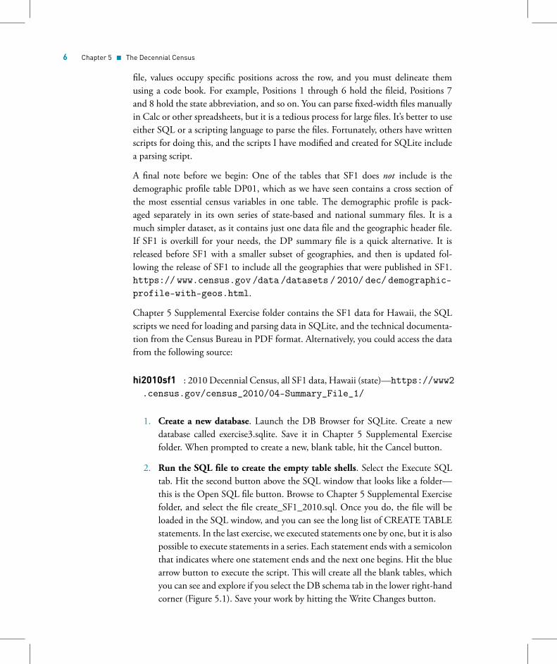
file, values occupy specific positions across the row, and you must delineate themusing a code book. For example, Positions 1 through 6 hold the fileid, Positions 7and 8 hold the state abbreviation, and so on. You can parse fixed-width files manuallyin Calc or other spreadsheets, but it is a tedious process for large files. It’s better to useeither SQL or a scripting language to parse the files. Fortunately, others have writtenscripts for doing this, and the scripts I have modified and created for SQLite includea parsing script.
A final note before we begin: One of the tables that SF1 does not include is thedemographic profile table DP01, which as we have seen contains a cross section ofthe most essential census variables in one table. The demographic profile is pack-aged separately in its own series of state-based and national summary files. It is amuch simpler dataset, as it contains just one data file and the geographic header file.If SF1 is overkill for your needs, the DP summary file is a quick alternative. It isreleased before SF1 with a smaller subset of geographies, and then is updated fol-lowing the release of SF1 to include all the geographies that were published in SF1.https:// www.census.gov /data /datasets / 2010/ dec/ demographic-profile-with-geos.html.
Chapter 5 Supplemental Exercise folder contains the SF1 data for Hawaii, the SQLscripts we need for loading and parsing data in SQLite, and the technical documenta-tion from the Census Bureau in PDF format. Alternatively, you could access the datafrom the following source:
hi2010sf1 : 2010 Decennial Census, all SF1 data, Hawaii (state)—https://www2.census.gov/census_2010/04-Summary_File_1/
1. Create a new database. Launch the DB Browser for SQLite. Create a newdatabase called exercise3.sqlite. Save it in Chapter 5 Supplemental Exercisefolder. When prompted to create a new, blank table, hit the Cancel button.
2. Run the SQL file to create the empty table shells. Select the Execute SQLtab. Hit the second button above the SQL window that looks like a folder—this is the Open SQL file button. Browse to Chapter 5 Supplemental Exercisefolder, and select the file create_SF1_2010.sql. Once you do, the file will beloaded in the SQL window, and you can see the long list of CREATE TABLEstatements. In the last exercise, we executed statements one by one, but it is alsopossible to execute statements in a series. Each statement ends with a semicolonthat indicates where one statement ends and the next one begins. Hit the bluearrow button to execute the script. This will create all the blank tables, whichyou can see and explore if you select the DB schema tab in the lower right-handcorner (Figure 5.1). Save your work by hitting the Write Changes button.

Chapter 5 � The Decennial Census 7
FIGURE 5.1 LOAD AND RUN SCRIPT TO CREATE SF1 TABLES
3. Load the first population file. Go to File—Import—Table From CSV File.Browse to Chapter 5 Supplemental Exercise hi2010sf1 folder. At the bottomof the screen, change the option from Text files to All files (even thoughthe data files are in a CSV format, their file extension is .sf1, so they don’tappear when looking for files with the .csv extension). Select the first sf1file hi000012010.sf1, and hit Open. Under table name, change the name tosf1_00001. The field separator should be a comma. Uncheck the box that saysColumn names in first line, but check the box to Trim fields (Figure 5.2). HitOK. You’ll get prompted with a message that says “There is already a tablewith that name. Do you want to import data into it?” Click Yes. The data willimport. When it’s finished, hit the Browse tab, and in the table drop down,select table sf1_00001. You should see all the data has been imported into theempty table. Save your work.
4. Load the next two population files. Repeat the previous step and load in thenext two population files, file hi000022010.sf1 into table sf1_00002 and filehi000032010.sf1 into table sf1_00003.
5. Create staging table for geographic headers. Getting the geographic headerfile into the database is a two-step process. First, we’ll load the fixed-width fileinto a temporary table where we store everything in a single field. Hit the SQLtab, and hit the first button above the window to add a new SQL window.

8 Chapter 5 � The Decennial Census
FIGURE 5.2 IMPORT FIRST SF1 TABLE
Then close the window that had our creation script by hitting the X. Writethis statement in the empty window:
CREATE TABLE geo_header_staging (data TEXT);
Then import the geographic header file higeo2010.sf1 (last file in the file list)into the geo_header_staging table. In the import window, change the tablename to geo_header_staging, change the field separator option to Other, andleave it blank. Also uncheck the trim fields box (Figure 5.3). When finished,browse the table to make sure the data was imported.
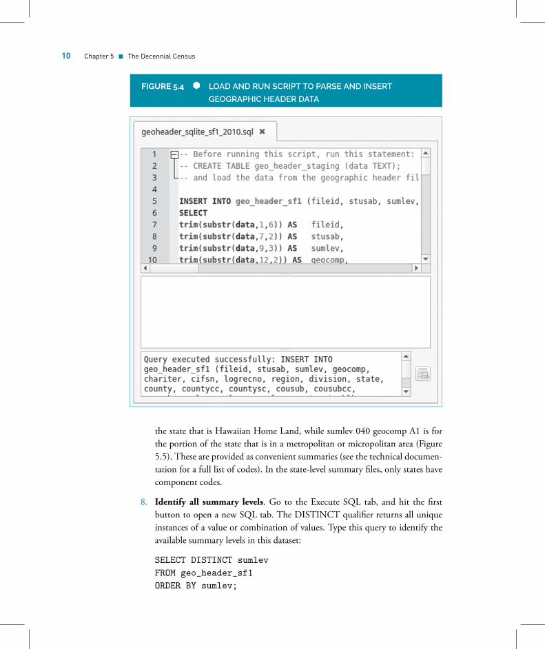
6. Parse and load the geo header data into the permanent table. Go to the Ex-ecute SQL tab, and erase the previous statement. Hit the open SQL file button(second button), and select the geoheader_sqlite_sf1_2010.sql file to load thescript into the SQL window. Hit the execute button (Figure 5.4). This scripttakes each row in the staging table and splits it into individual values to fit intothe geo_header_sf1 table. The values are split using the substring function thatwe saw earlier at designated positions based on the Census Bureau’s documen-tation. We also use a function called trim to remove blank spaces before or after

Chapter 5 � The Decennial Census 9
FIGURE 5.3 IMPORT GEOGRAPHIC HEADER FILE
each value and, in some cases, a function called cast to convert values from onedata type to another (in this case text to integers).
7. Browse the geo_header_sf1 table. Browse the data for geo_header_sf1. Clickon the sumlev column to sort the data by summary level. This table con-tains records for every piece of geography in Hawaii that nests fully (and insome cases partially) within the state. Remember the summary level codesfrom Chapter 3? Code 040 is for the state level. The first record with sumlev040 and geocomp 00 is for the state as a whole. The geocomp field indicateswhether the record pertains to a specific geographic component of the area, forexample, sumlev 040 geocomp 95 indicates this record is for the portion of
10 Chapter 5 � The Decennial Census
FIGURE 5.4 LOAD AND RUN SCRIPT TO PARSE AND INSERT
GEOGRAPHIC HEADER DATA
the state that is Hawaiian Home Land, while sumlev 040 geocomp A1 is forthe portion of the state that is in a metropolitan or micropolitan area (Figure5.5). These are provided as convenient summaries (see the technical documen-tation for a full list of codes). In the state-level summary files, only states havecomponent codes.
8. Identify all summary levels. Go to the Execute SQL tab, and hit the firstbutton to open a new SQL tab. The DISTINCT qualifier returns all uniqueinstances of a value or combination of values. Type this query to identify theavailable summary levels in this dataset:
SELECT DISTINCT sumlevFROM geo_header_sf1ORDER BY sumlev;
Chapter 5 � The Decennial Census 11
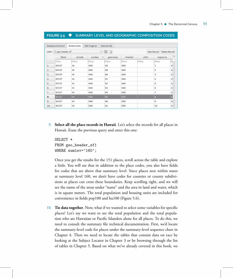
FIGURE 5.5 SUMMARY LEVEL AND GEOGRAPHIC COMPOSITION CODES
9. Select all the place records in Hawaii. Let’s select the records for all places inHawaii. Erase the previous query and enter this one:
SELECT *FROM geo_header_sf1WHERE sumlev=’160’;
Once you get the results for the 151 places, scroll across the table and explorea little. You will see that in addition to the place codes, you also have fieldsfor codes that are above that summary level. Since places nest within statesat summary level 160, we don’t have codes for counties or county subdivi-sions as places can cross these boundaries. Keep scrolling right, and we willsee the name of the areas under “name” and the area in land and water, whichis in square meters. The total population and housing units are included forconvenience in fields pop100 and hu100 (Figure 5.6).
10. Tie data together. Now, what if we wanted to select some variables for specificplaces? Let’s say we want to see the total population and the total popula-tion who are Hawaiian or Pacific Islanders alone for all places. To do this, weneed to consult the summary file technical documentation. First, we’d locatethe summary-level code for places under the summary-level sequence chart inChapter 4. Then we need to locate the tables that contain data on race bylooking at the Subject Locator in Chapter 3 or by browsing through the listof tables in Chapter 5. Based on what we’ve already covered in this book, we
12 Chapter 5 � The Decennial Census
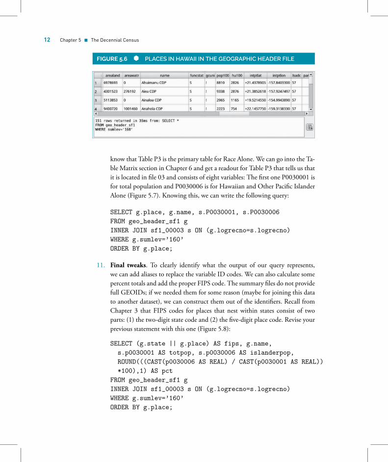
FIGURE 5.6 PLACES IN HAWAII IN THE GEOGRAPHIC HEADER FILE
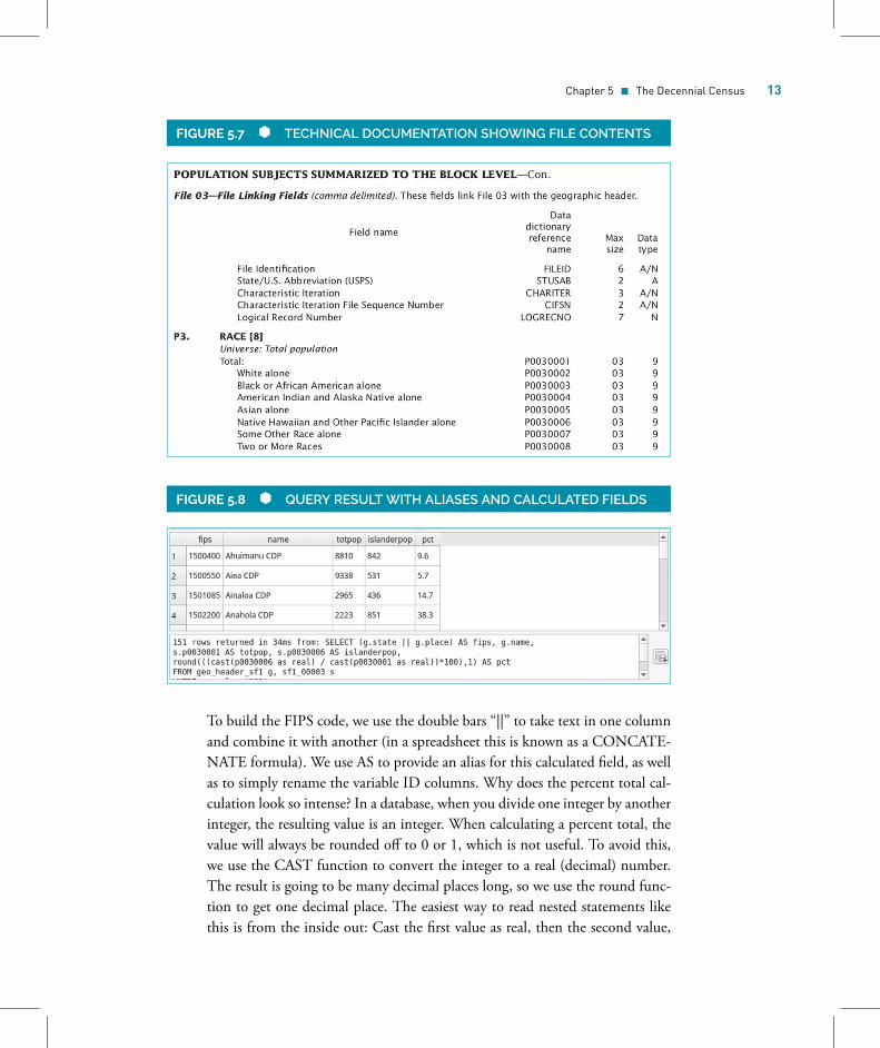
know that Table P3 is the primary table for Race Alone. We can go into the Ta-ble Matrix section in Chapter 6 and get a readout for Table P3 that tells us thatit is located in file 03 and consists of eight variables: The first one P0030001 isfor total population and P0030006 is for Hawaiian and Other Pacific IslanderAlone (Figure 5.7). Knowing this, we can write the following query:
SELECT g.place, g.name, s.P0030001, s.P0030006FROM geo_header_sf1 gINNER JOIN sf1_00003 s ON (g.logrecno=s.logrecno)WHERE g.sumlev=’160’ORDER BY g.place;
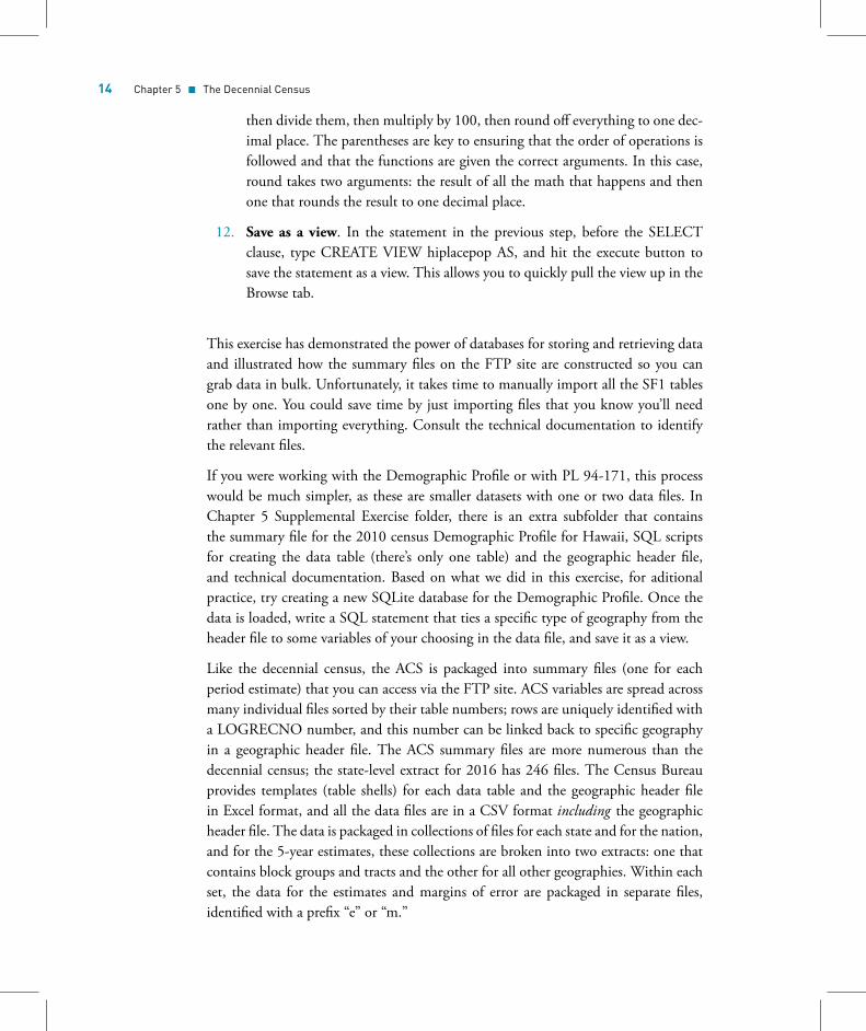
11. Final tweaks. To clearly identify what the output of our query represents,we can add aliases to replace the variable ID codes. We can also calculate somepercent totals and add the proper FIPS code. The summary files do not providefull GEOIDs; if we needed them for some reason (maybe for joining this datato another dataset), we can construct them out of the identifiers. Recall fromChapter 3 that FIPS codes for places that nest within states consist of twoparts: (1) the two-digit state code and (2) the five-digit place code. Revise yourprevious statement with this one (Figure 5.8):
SELECT (g.state || g.place) AS fips, g.name,s.p0030001 AS totpop, s.p0030006 AS islanderpop,ROUND(((CAST(p0030006 AS REAL) / CAST(p0030001 AS REAL))*100),1) AS pct
FROM geo_header_sf1 gINNER JOIN sf1_00003 s ON (g.logrecno=s.logrecno)WHERE g.sumlev=’160’ORDER BY g.place;
Chapter 5 � The Decennial Census 13
FIGURE 5.7 TECHNICAL DOCUMENTATION SHOWING FILE CONTENTS
FIGURE 5.8 QUERY RESULTWITH ALIASES AND CALCULATED FIELDS
To build the FIPS code, we use the double bars “||” to take text in one columnand combine it with another (in a spreadsheet this is known as a CONCATE-NATE formula). We use AS to provide an alias for this calculated field, as wellas to simply rename the variable ID columns. Why does the percent total cal-culation look so intense? In a database, when you divide one integer by anotherinteger, the resulting value is an integer. When calculating a percent total, thevalue will always be rounded off to 0 or 1, which is not useful. To avoid this,we use the CAST function to convert the integer to a real (decimal) number.The result is going to be many decimal places long, so we use the round func-tion to get one decimal place. The easiest way to read nested statements likethis is from the inside out: Cast the first value as real, then the second value,
14 Chapter 5 � The Decennial Census
then divide them, then multiply by 100, then round off everything to one dec-imal place. The parentheses are key to ensuring that the order of operations isfollowed and that the functions are given the correct arguments. In this case,round takes two arguments: the result of all the math that happens and thenone that rounds the result to one decimal place.
12. Save as a view. In the statement in the previous step, before the SELECTclause, type CREATE VIEW hiplacepop AS, and hit the execute button tosave the statement as a view. This allows you to quickly pull the view up in theBrowse tab.
This exercise has demonstrated the power of databases for storing and retrieving dataand illustrated how the summary files on the FTP site are constructed so you cangrab data in bulk. Unfortunately, it takes time to manually import all the SF1 tablesone by one. You could save time by just importing files that you know you’ll needrather than importing everything. Consult the technical documentation to identifythe relevant files.
If you were working with the Demographic Profile or with PL 94-171, this processwould be much simpler, as these are smaller datasets with one or two data files. InChapter 5 Supplemental Exercise folder, there is an extra subfolder that containsthe summary file for the 2010 census Demographic Profile for Hawaii, SQL scriptsfor creating the data table (there’s only one table) and the geographic header file,and technical documentation. Based on what we did in this exercise, for aditionalpractice, try creating a new SQLite database for the Demographic Profile. Once thedata is loaded, write a SQL statement that ties a specific type of geography from theheader file to some variables of your choosing in the data file, and save it as a view.
Like the decennial census, the ACS is packaged into summary files (one for eachperiod estimate) that you can access via the FTP site. ACS variables are spread acrossmany individual files sorted by their table numbers; rows are uniquely identified witha LOGRECNO number, and this number can be linked back to specific geographyin a geographic header file. The ACS summary files are more numerous than thedecennial census; the state-level extract for 2016 has 246 files. The Census Bureauprovides templates (table shells) for each data table and the geographic header filein Excel format, and all the data files are in a CSV format including the geographicheader file. The data is packaged in collections of files for each state and for the nation,and for the 5-year estimates, these collections are broken into two extracts: one thatcontains block groups and tracts and the other for all other geographies. Within eachset, the data for the estimates and margins of error are packaged in separate files,identified with a prefix “e” or “m.”
Chapter 5 � The Decennial Census 15
While the Census Bureau provides easy-to-follow instructions for importing an in-dividual data file into one of the Excel templates, using a spreadsheet to work withthis data is tough. For a particular ACS table, you would need to import at least threefiles—(1) the geographic header, (2) the estimate table, and (3) the margin of errortable—and would use VLOOKUP formulas to tie them together. This is fine if youneed a couple of tables for all geographies, but this is not a feasible approach for work-ing with a lot of data, or even a few variables scattered across many files. It still wouldbe better to import the files into a database or a statistical package. Besides Excel,the Census Bureau provides table structures in a CSV and SAS format (SAS pro-grammers can use preassembled macros). As before, you could also search github forscripts for generating tables in SQL or another stat package. The best launching pointfor accessing the ACS summary files is from the ACS technical documentation page:https://www.census.gov/programs-surveys/acs/technical-documentation/summary-file-documentation.html.
6THE AMERICAN
COMMUNITY SURVEY
6.4 EXERCISESRanking ACS Data and Testing for Statistical DifferenceCensus data is commonly used to categorize and rank places. As we have discussed,the census is used to distribute hundreds of billions of dollars in federal aid. In theircase study of three federal programs, Nesse and Rahe (2015) found than none ofthe programs incorporated the margin of error (MOE) for American CommunitySurvey (ACS) estimates into their calculations. In this exercise, we will explore theimpact the MOE has on rankings and will get some more practice with aggregatingvalues.
We will use one of the programs from this study in our example. The U.S. Depart-ment of Agriculture (USDA) runs the Supplemental Nutrition Assistance Program(SNAP), which provides food stamps to individuals in need. Funding is distributedto each of the states based on a variety of criteria and formulas. One aspect of thefunding mechanism is the award of performance bonuses to states that do the bestjob at administering the program. Four different evaluation categories are used toadminister bonuses, and one of them relies on census data. The Program Access In-dex (PAI) is used to award $12 million to eight states: the four states that have thehighest index value and the four states that showed the most improvement in theirindex compared with the previous year. Nine states receive awards in the event of atie, and the money is divided in the same manner as it would be for eight states. Ifa state is among the top four in both the best category and best improved category,
16
Chapter 6 � The American Community Survey 17
that state receives only one award and the fifth best state is granted an award to bringthe number up to eight.
The index is calculated for each state by dividing the average number of SNAP recip-ients in a month by the total population living below 125% of the poverty line in acalendar year. The data on poverty is from the 1-year ACS, while the data on SNAPrecipients comes from the USDA’s administrative records (the ACS includes data onSNAP recipients, but it’s published at the household level, while the USDA’s data is atthe person level). The USDA makes a number of adjustments prior to calculating theindex. The number of SNAP recipients is adjusted by deducting people who receivedbenefits as part of disaster assistance and participants in the Food Distribution Pro-gram on Indian Reservations (FDPIR). The number of people in poverty is adjustedby deducting the number of average monthly participants in FDPIR and the totalnumber of low-income Supplemental Security Income (SSI) recipients in California(U.S. Department of Agriculture, 2018).
In our example, we will account for the MOE in the calculations to create adjustedpoverty estimates and the index. We will look at the rankings and identify the topfour states in the best program category and will run the statistical difference testto see if the values between the fourth- and fifth-best state are truly different. TheUSDA publishes a thorough summary of the data used and statistics generated in anannual report USDA (2018). I created a spreadsheet that contains the necessary datafor making the poverty adjustments and calculating the index by copying the relevantcolumns out of the report and pasting them into the workbook. We will import thepoverty data from the ACS so that we get the MOEs (as they are not included in thereport). The data is available in the Chapter 6 Supplementary Exercise folder, or youcan obtain it from the following source:
B17002 Ratio of Income to Poverty Level in the Past 12 Months: 2016 ACS,All states in the United States (state)—https://data.census.gov/
Calculating the SNAP Program Access Index: A Step-By-Step Guide: UDSA,2016 report—https://www.fns.usda.gov/snap/calculating-supple-mental-nutrition-assistance-program-snap-program-access-index-step-step-guide
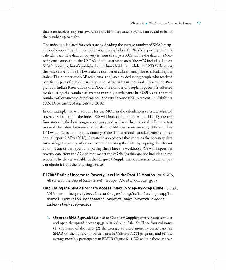
1. Open the SNAP spreadsheet. Go to Chapter 6 Supplementary Exercise folderand open the spreadsheet snap_pai2016.xlsx in Calc. You’ll see four columns:(1) the name of the state, (2) the average adjusted monthly participants inSNAP, (3) the number of participants in California’s SSI program, and (4) theaverage monthly participants in FDPIR (Figure 6.1). We will use these last two
18 Chapter 6 � The American Community Survey
FIGURE 6.1 2016 USDA SNAP PROGRAM ACCESS
INDEX COMPONENTS
FIGURE 6.2 ACS TABLE B17002 RATIO OF INCOME TO
POVERTY LEVEL
columns to adjust our poverty numbers. Note that the UDSA excluded NewMexico from the rankings in 2016 due to some data quality issue.
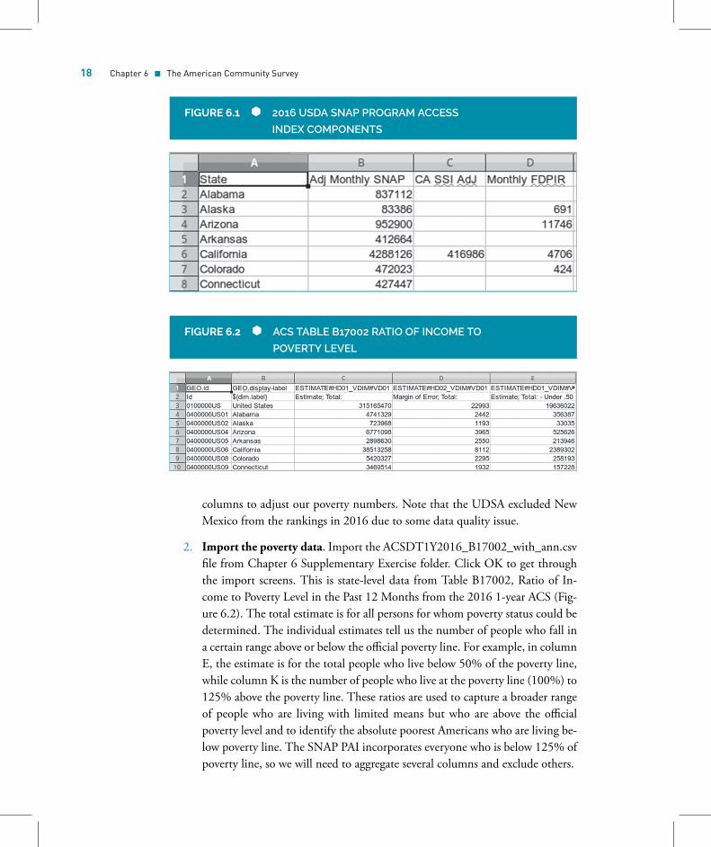
2. Import the poverty data. Import the ACSDT1Y2016_B17002_with_ann.csvfile from Chapter 6 Supplementary Exercise folder. Click OK to get throughthe import screens. This is state-level data from Table B17002, Ratio of In-come to Poverty Level in the Past 12 Months from the 2016 1-year ACS (Fig-ure 6.2). The total estimate is for all persons for whom poverty status could bedetermined. The individual estimates tell us the number of people who fall ina certain range above or below the official poverty line. For example, in columnE, the estimate is for the total people who live below 50% of the poverty line,while column K is the number of people who live at the poverty line (100%) to125% above the poverty line. These ratios are used to capture a broader rangeof people who are living with limited means but who are above the officialpoverty level and to identify the absolute poorest Americans who are living be-low poverty line. The SNAP PAI incorporates everyone who is below 125% ofpoverty line, so we will need to aggregate several columns and exclude others.
Chapter 6 � The American Community Survey 19
3. Remove unnecessary columns and rows. Delete columns M through AB, asthese fall outside the range we need. Then delete columns C and D as wedon’t need the totals. Delete the first row that contains the IDs, then delete thesummary row for the United States. Scroll down to the bottom of the sheetand delete the row for Puerto Rico (since it’s not a state, it doesn’t partici-pate in SNAP). Save your work by doing Save As, and save the file in a newspreadsheet called exercise2.
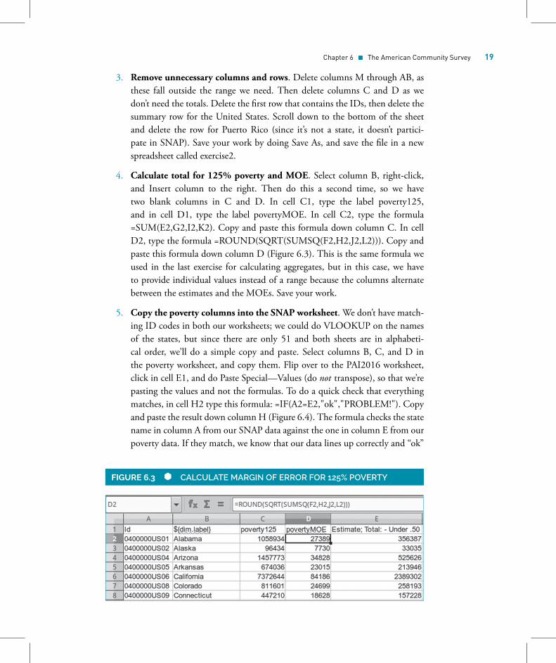
4. Calculate total for 125% poverty and MOE. Select column B, right-click,and Insert column to the right. Then do this a second time, so we havetwo blank columns in C and D. In cell C1, type the label poverty125,and in cell D1, type the label povertyMOE. In cell C2, type the formula=SUM(E2,G2,I2,K2). Copy and paste this formula down column C. In cellD2, type the formula =ROUND(SQRT(SUMSQ(F2,H2,J2,L2))). Copy andpaste this formula down column D (Figure 6.3). This is the same formula weused in the last exercise for calculating aggregates, but in this case, we haveto provide individual values instead of a range because the columns alternatebetween the estimates and the MOEs. Save your work.
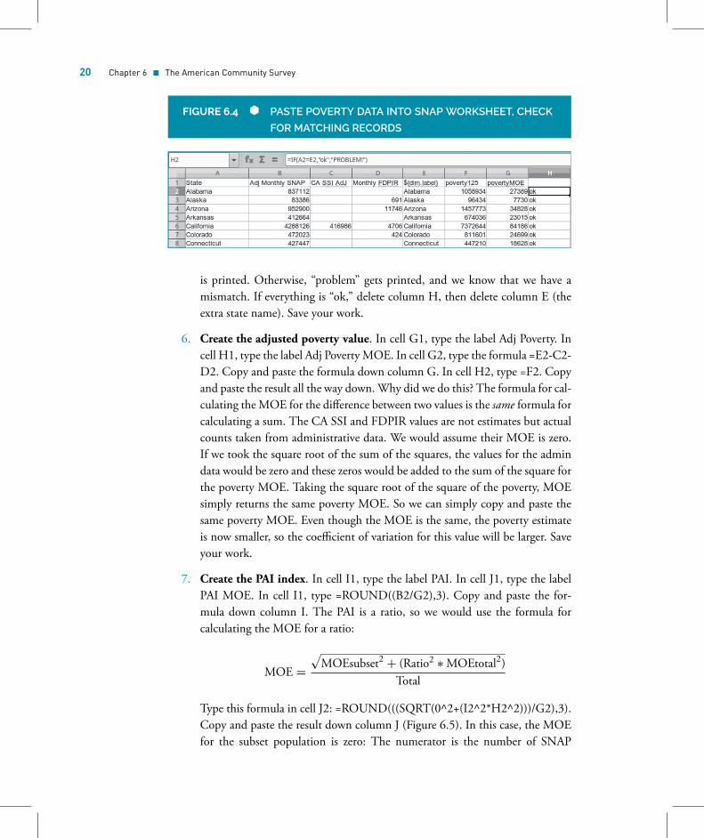
5. Copy the poverty columns into the SNAP worksheet. We don’t have match-ing ID codes in both our worksheets; we could do VLOOKUP on the namesof the states, but since there are only 51 and both sheets are in alphabeti-cal order, we’ll do a simple copy and paste. Select columns B, C, and D inthe poverty worksheet, and copy them. Flip over to the PAI2016 worksheet,click in cell E1, and do Paste Special—Values (do not transpose), so that we’repasting the values and not the formulas. To do a quick check that everythingmatches, in cell H2 type this formula: =IF(A2=E2,"ok","PROBLEM!"). Copyand paste the result down columnH (Figure 6.4). The formula checks the statename in column A from our SNAP data against the one in column E from ourpoverty data. If they match, we know that our data lines up correctly and “ok”
FIGURE 6.3 CALCULATE MARGIN OF ERROR FOR 125% POVERTY
20 Chapter 6 � The American Community Survey
FIGURE 6.4 PASTE POVERTY DATA INTO SNAP WORKSHEET, CHECK
FOR MATCHING RECORDS
is printed. Otherwise, “problem” gets printed, and we know that we have amismatch. If everything is “ok,” delete column H, then delete column E (theextra state name). Save your work.
6. Create the adjusted poverty value. In cell G1, type the label Adj Poverty. Incell H1, type the label Adj PovertyMOE. In cell G2, type the formula =E2-C2-D2. Copy and paste the formula down column G. In cell H2, type =F2. Copyand paste the result all the way down.Why did we do this? The formula for cal-culating theMOE for the difference between two values is the same formula forcalculating a sum. The CA SSI and FDPIR values are not estimates but actualcounts taken from administrative data. We would assume their MOE is zero.If we took the square root of the sum of the squares, the values for the admindata would be zero and these zeros would be added to the sum of the square forthe poverty MOE. Taking the square root of the square of the poverty, MOEsimply returns the same poverty MOE. So we can simply copy and paste thesame poverty MOE. Even though the MOE is the same, the poverty estimateis now smaller, so the coefficient of variation for this value will be larger. Saveyour work.
7. Create the PAI index. In cell I1, type the label PAI. In cell J1, type the labelPAI MOE. In cell I1, type =ROUND((B2/G2),3). Copy and paste the for-mula down column I. The PAI is a ratio, so we would use the formula forcalculating the MOE for a ratio:
MOE =√MOEsubset2 + (Ratio2 ∗ MOEtotal2)
Total
Type this formula in cell J2: =ROUND(((SQRT(0^2+(I2^2*H2^2)))/G2),3).Copy and paste the result down column J (Figure 6.5). In this case, the MOEfor the subset population is zero: The numerator is the number of SNAP
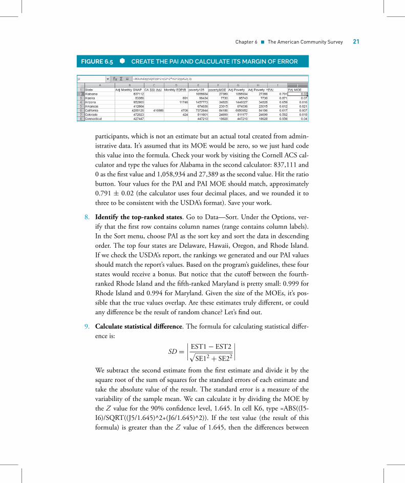
Chapter 6 � The American Community Survey 21
FIGURE 6.5 CREATE THE PAI AND CALCULATE ITS MARGIN OF ERROR
participants, which is not an estimate but an actual total created from admin-istrative data. It’s assumed that its MOE would be zero, so we just hard codethis value into the formula. Check your work by visiting the Cornell ACS cal-culator and type the values for Alabama in the second calculator: 837,111 and0 as the first value and 1,058,934 and 27,389 as the second value. Hit the ratiobutton. Your values for the PAI and PAI MOE should match, approximately0.791 ± 0.02 (the calculator uses four decimal places, and we rounded it tothree to be consistent with the USDA’s format). Save your work.
8. Identify the top-ranked states. Go to Data—Sort. Under the Options, ver-ify that the first row contains column names (range contains column labels).In the Sort menu, choose PAI as the sort key and sort the data in descendingorder. The top four states are Delaware, Hawaii, Oregon, and Rhode Island.If we check the USDA’s report, the rankings we generated and our PAI valuesshould match the report’s values. Based on the program’s guidelines, these fourstates would receive a bonus. But notice that the cutoff between the fourth-ranked Rhode Island and the fifth-ranked Maryland is pretty small: 0.999 forRhode Island and 0.994 for Maryland. Given the size of the MOEs, it’s pos-sible that the true values overlap. Are these estimates truly different, or couldany difference be the result of random chance? Let’s find out.
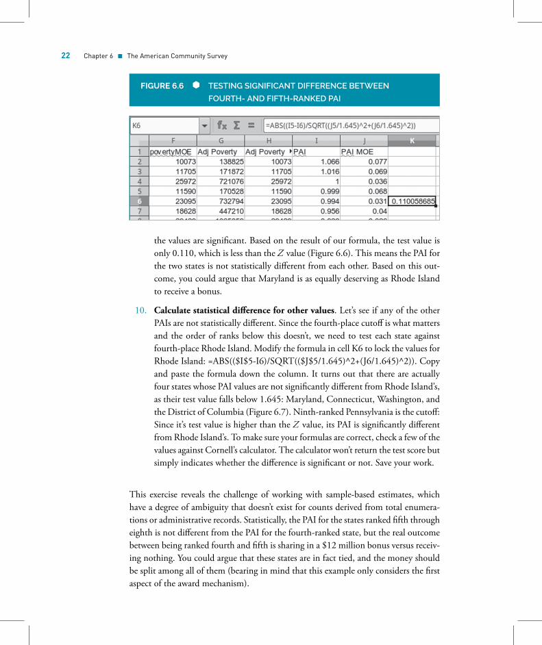
9. Calculate statistical difference. The formula for calculating statistical differ-ence is:
SD =∣∣∣∣ EST1 − EST2√
SE12 + SE22
∣∣∣∣We subtract the second estimate from the first estimate and divide it by thesquare root of the sum of squares for the standard errors of each estimate andtake the absolute value of the result. The standard error is a measure of thevariability of the sample mean. We can calculate it by dividing the MOE bythe Z value for the 90% confidence level, 1.645. In cell K6, type =ABS((I5-I6)/SQRT((J5/1.645)^2+(J6/1.645)^2)). If the test value (the result of thisformula) is greater than the Z value of 1.645, then the differences between
22 Chapter 6 � The American Community Survey
FIGURE 6.6 TESTING SIGNIFICANT DIFFERENCE BETWEEN
FOURTH- AND FIFTH-RANKED PAI
the values are significant. Based on the result of our formula, the test value isonly 0.110, which is less than the Z value (Figure 6.6). This means the PAI forthe two states is not statistically different from each other. Based on this out-come, you could argue that Maryland is as equally deserving as Rhode Islandto receive a bonus.
10. Calculate statistical difference for other values. Let’s see if any of the otherPAIs are not statistically different. Since the fourth-place cutoff is what mattersand the order of ranks below this doesn’t, we need to test each state againstfourth-place Rhode Island. Modify the formula in cell K6 to lock the values forRhode Island: =ABS(($I$5-I6)/SQRT(($J$5/1.645)^2+(J6/1.645)^2)). Copyand paste the formula down the column. It turns out that there are actuallyfour states whose PAI values are not significantly different from Rhode Island’s,as their test value falls below 1.645: Maryland, Connecticut, Washington, andthe District of Columbia (Figure 6.7). Ninth-ranked Pennsylvania is the cutoff:Since it’s test value is higher than the Z value, its PAI is significantly differentfrom Rhode Island’s. To make sure your formulas are correct, check a few of thevalues against Cornell’s calculator. The calculator won’t return the test score butsimply indicates whether the difference is significant or not. Save your work.
This exercise reveals the challenge of working with sample-based estimates, whichhave a degree of ambiguity that doesn’t exist for counts derived from total enumera-tions or administrative records. Statistically, the PAI for the states ranked fifth througheighth is not different from the PAI for the fourth-ranked state, but the real outcomebetween being ranked fourth and fifth is sharing in a $12 million bonus versus receiv-ing nothing. You could argue that these states are in fact tied, and the money shouldbe split among all of them (bearing in mind that this example only considers the firstaspect of the award mechanism).

Chapter 6 � The American Community Survey 23
FIGURE 6.7 PAI VALUES THAT ARE NOT SIGNIFICANTLY DIFFERENT
FROM THE FOURTH-RANKED VALUE
Under federal regulations, the USDA has flexibility in deciding what criteria to use,how to generate the index, and how to award the bonuses based on the outcome. Weare not saying that they are violating the regulations. For example, the regulationsspecify that they should use 130% of poverty as a ratio, but they use 125% as theformer value is not published by the Census Bureau. The USDA previously usedpoverty estimates from the Current Population Survey but switched to the ACS asthe estimates were more precise. One could argue that the rank and thus the award isbased on the median value of the interval, regardless of what the MOE is. In publicpolicy, there is always a trade-off between being statistically precise and using a simplermethod that more people can grasp and thus agree with.
One final note: You should only create derived values for geographies (like the neigh-borhood in our first exercise in Chapter 6) or categories (like the PAI in this exercise)that do not already exist. There’s no need to aggregate values for census tracts tocounties because the Census Bureau has already created these estimates. In this ex-ercise, the value that we calculated for the number of people below 125% povertywas actually already published in another table—summary table S1701 Poverty Sta-tus in the last 12 months (this table has a lot more variables in it relative to the tablewe used). The MOEs for published census estimates are often more precise than theones we calculate ourselves. That’s because the Census Bureau generates its estimatesdirectly from the individual sample records, while our estimates are derived from totalestimates. For example, the number of people below 125% poverty in Alabama was1,058,934 in the 1-year 2016 ACS. Our derived MOE for this estimate was 27,389,but in the Census Bureau’s published table, it was 26,546. In circumstances like thisexercise, where a small difference could translate to getting millions of dollars or not,we’d want to use the most accurate estimates possible (but in this case, it was betterthat you got additional practice aggregating the data yourself!).
11CENSUS DATA DERIVATIVES
11.4 MEANS AND MEDIANSFOR AGGREGATES
Calculating a new median for aggregates is more complex than calculating a newmean, but we will walk through each step since the process is not widely documented.Remember that the median value represents the case that falls in the center of adistribution. To calculate a new median, we would need to combine the records ofindividual respondents from these two census tracts, sort them, and select the middlevalue. This isn’t possible as we only have access to summarized data. The solutionis to use a method called statistical interpolation, where we can derive the medianbased on ranges of data. The Census Bureau publishes interval data for a number ofvariables, such as Table B19001 Household Income, where the number of householdsare counted by income brackets.
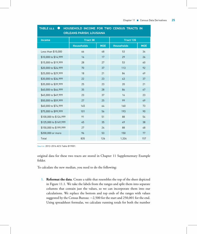
The California State Data Center (2016) published a brief tutorial demonstratinghow to calculate a derived median and its associated margin of error (MOE). Thefollowing steps are based on their example, using our two New Orleans census tracts.The published 2012–2016 medians for the tracts are $68,780 (±5,160) and $64,333(±12,774), respectively. Table 11.1 is the original household income table for thesetwo tracts. We would aggregate this data for the two tracts using the techniqueslearned in Chapter 6. Figure 11.1 displays what the final layout of the spreadsheetshould look like, and we will refer to it throughout the example. The top of the sheetin this figure displays how the aggregated household data should be reformatted (inthe first step), while the bottom of the sheet shows the results of the formulas for eachof the steps that we’ll take below. The cells that are highlighted in the figure repre-sent values that are used in the calculations. A copy of this spreadsheet as well as the
24
Chapter 11 � Census Data Derivatives 25
TABLE 11.1 HOUSEHOLD INCOME FOR TWO CENSUS TRACTS IN
ORLEANS PARISH, LOUSIANA
Income Tract 38 Tract 135
Households MOE Households MOE
Less than $10,000 66 48 53 34
$10,000 to $14,999 16 17 29 26
$15,000 to $19,999 28 27 53 60
$20,000 to $24,999 70 37 113 92
$25,000 to $29,999 18 21 84 49
$30,000 to $34,999 22 23 43 37
$35,000 to $39,999 25 23 20 21
$40,000 to $44,999 35 28 86 67
$45,000 to $49,999 23 37 16 23
$50,000 to $59,999 27 25 99 49
$60,000 to $74,999 145 64 160 73
$75,000 to $99,999 101 56 193 90
$100,000 to $124,999 91 51 88 54
$125,000 to $149,999 45 35 49 38
$150,000 to $199,999 27 24 88 48
$200,000 or more 96 53 150 77
Total 835 126 1,324 157
Source: 2012–2016 ACS Table B19001.
original data for these two tracts are stored in Chapter 11 Supplementary Examplefolder.
To calculate the new median, you need to do the following:
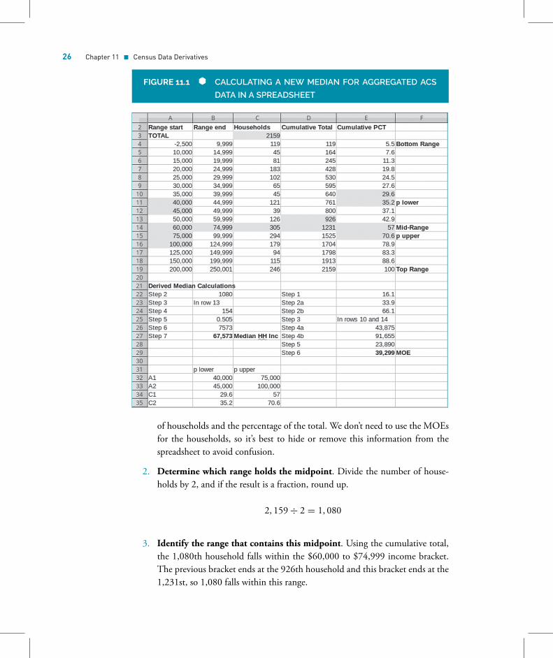
1. Reformat the data. Create a table that resembles the top of the sheet depictedin Figure 11.1. We take the labels from the ranges and split them into separatecolumns that contain just the values, so we can incorporate them into ourcalculations. We replace the bottom and top ends of the ranges with valuessuggested by the Census Bureau:−2,500 for the start and 250,001 for the end.Using spreadsheet formulas, we calculate running totals for both the number
26 Chapter 11 � Census Data Derivatives
FIGURE 11.1 CALCULATING A NEW MEDIAN FOR AGGREGATED ACS
DATA IN A SPREADSHEET
of households and the percentage of the total. We don’t need to use the MOEsfor the households, so it’s best to hide or remove this information from thespreadsheet to avoid confusion.
2. Determine which range holds the midpoint. Divide the number of house-holds by 2, and if the result is a fraction, round up.
2, 159 ÷ 2 = 1, 080
3. Identify the range that contains this midpoint. Using the cumulative total,the 1,080th household falls within the $60,000 to $74,999 income bracket.The previous bracket ends at the 926th household and this bracket ends at the1,231st, so 1,080 falls within this range.
Chapter 11 � Census Data Derivatives 27
4. Calculate how many households in the midrange are needed to reach themidpoint. We subtract the number of households from the previous rangefrom the midpoint.
1, 080 − 926 = 154
5. Calculate the proportion of the number of households in the midrange(60,000–74,999) that are needed to get to the midpoint. Using the resultfrom the previous step and the number of households in the midrange,
154 ÷ 305 = 0.505
6. Apply this proportion to the width of the midrange dollar values. First, wecalculate the width, then we apply the proportion:
(74, 999 − 60, 000) ∗ 0.505 = 7, 573
7. Calculate the new median. Using the beginning of the midrange and theresult from the last step:
60, 000 + 7, 573 = $67, 573
This result is close to the medians of the individual tracts, so this outcome seems rea-sonable. Calculating the MOE is more involved and uses formulas that are typicallyemployed when creating derivatives of public use microdata.
1. Approximate the standard error of a 50% proportion. The formula for thisis printed below, where B represents the total number of households (the base)and DF is the design factor from the Public Use Microdate Samples (PUMS)files. The DF is a table of constants published for different variables at thenational level and for individual states. We’ll discuss the source for these vari-ables at the end; the DF for income variables for the State of Louisiana in2012–2016 is 1.5:
SE(50%) = DF ∗√99B
∗ 502
1.5 ∗√
992, 159
∗ 502 = 16.1
28 Chapter 11 � Census Data Derivatives
2. Subtract and add the standard error from the last step to 50%. This willgive us the lower and upper bounds.
p_lower = 50 − 16.1 = 33.9
p_upper = 50 + 16.1 = 66.1
3. Identify the ranges in the distribution that contain the lower and upperbounds. Using the cumulative percentages, 33.9 (p_lower) falls within the40,000 to 44,999 range; the previous range stops at 29.6, and this range stopsat 35.2, so 33.9 falls within it. The 75,000 to 99,999 range contains 66.1(p_upper). Note that it is possible that your lower and upper bounds could fallwithin the same range; we’ll discuss this variation at the end.
4. Approximate the lower and upper bounds for a confidence interval aboutthe median. To do this, we need to identify these four variables for each of thebounds:
a. A1: the smallest value in the range (40,000 for p_lower and 75,000 forp_upper)
b. A2: the smallest value in the next higher range (45,000 for p_lower and100,000 for p_upper)
c. C1: the cumulative percentage of households less than the A1 range(29.6 for p_lower and 57.0 for p_upper)
d. C2: the cumulative percentage of households less than the A2 range(35.2 for p_lower and 70.6 for p_upper)
In your spreadsheet, it’s helpful to explicitly label these values as depicted inthe bottom of Figure 11.1, as this can help you avoid mistakes. Instead of hardcoding the value beside the label, you can provide a reference to the cell thatcontains it, that is, =“cell value.” Once you’ve identified the values, you caninsert them into this formula and calculate the lower and upper values:
Bound =(
p − C1C2 − C1
)∗ (A2 − A1) + A1
(33.9 − 29.635.2 − 29.6
)∗ (45, 000 − 40, 000) + 40, 000 = 43, 875
(66.1 − 5770.6 − 35.2
)∗ (100, 000 − 75, 000) + 75, 000 = 91, 655

Chapter 11 � Census Data Derivatives 29
5. Approximate the standard error of the median. Using the upper and lowerbounds from the last step:
0.5 ∗ (91, 655 − 43875) = 23, 890
6. Calculate the MOE. Remember from Chapter 6 that 1.645 is the constantthat applies to all ACS estimates, which are published at a 90% confidenceinterval:
1.645 ∗ 23, 890 = 39, 299
The median household income for these two census tracts combined is $67,573(±39,299). The MOE is quite high, but this isn’t unusual for this procedure. Theseinterpolation methods produce more conservative or higher MOEs than you wouldget if you were creating a median using the original, individual data values. If we usedthis procedure to calculate the median and MOE for a known published value, suchas income for one of the census tracts, the calculated estimate would differ and itsMOE would be higher.
One variation that you may encounter is that your bounds for p_lower and p_uppercould fall within the same value range. If this occurs, you would only need to createone set of A and C values in Step 4 and apply them to both the lower and upperbounds formula (so the only variable that would differ between the two formulaswould be the p_bound variable).
The Census Bureau publishes and annually updates the DF variables used in Step 1in technical documentation titled “Public Use Microdata Sample (PUMS) Accuracyof the Data” (U.S. Census Bureau, 2017). This documentation is published in PDFformat and is stored under the PUMS documentation section of the ACS website.Factors for each variable are published for the nation as a whole and each individualstate (including the District of Columbia and Puerto Rico) in the appendix of thisdocument. You will need to look up the appropriate factor for the specific year, state,and variables you’re working with. In this example, the DF for household or familyincome variables for Louisiana for 2012–2016 was 1.5; for the entire nation, thevariable is 1.6.

REFERENCES
California State Data Center. (2016, April). Re-calculating medians and their margin of errors foraggregated ACS data (January 2011 Network News,revised 2016). Sacramento: California State DataCenter, Demographic Research Unit. Retrieved fromhttp://www.dof.ca.gov/Forecasting/Demographics/Census_Data_Center_Network/.
Nesse, K., & Rahe, M. L. (2015). Conflicts in the use ofthe ACS by federal agencies between statutory require-ments and survey methodology. Population Research andPolicy Review, 34, 461–480.
U.S. Census Bureau. (2017). Public Use MicrodataSample PUMS accuracy of the data (2012–2016)(Tech. Rep.). Washington, DC: Author. Retrievedfrom https://www.census.gov/programs-surveys/acs/technical-documentation/pums/documentation.html.
U.S. Department of Agriculture. (2018, February). Cal-culating the Supplemental Nutrition Assistance Program(SNAP) Program Access Index: A step-by-step guide for2016 (Tech. Rep.). Washington, DC: Food and NutritionService. Retrieved from https://www.fns.usda.gov/snap/calculating-supplemental-nutrition-assistance-program-snap-program-access-index-step-step-guide.
0