Solid Earth, 2, 95–105, 2011www.solid-earth.net/2/95/2011/doi:10.5194/se-2-95-2011© Author(s) 2011. CC Attribution 3.0 License.

Solid Earth

Exploring the potentials and limitations of the time-reversalimaging of finite seismic sources

S. Kremers1, A. Fichtner1,*, G. B. Brietzke1,** , H. Igel1, C. Larmat2, L. Huang2, and M. Kaser1

1Department of Earth and Environmental Sciences, Ludwig-Maximilians-University, Theresienstr. 41/III,80333 Munich, Germany2EES-17 Geophysics Group, Los Alamos National Laboratory, Los Alamos, NM 87545, USA* now at: Faculty of Geosciences, Utrecht University, Utrecht, The Netherlands** now at: GFZ German Research Centre for Geosciences, Potsdam, Germany

Received: 28 January 2011 – Published in Solid Earth Discuss.: 17 March 2011Revised: 30 May 2011 – Accepted: 31 May 2011 – Published: 21 June 2011

Abstract. The characterisation of seismic sources with time-reversed wave fields is developing into a standard techniquethat has already been successful in numerous applications.While the time-reversal imaging of effective point sources isnow well-understood, little work has been done to extend thistechnique to the study of finite rupture processes. This is de-spite the pronounced non-uniqueness in classic finite sourceinversions.

The need to better constrain the details of finite ruptureprocesses motivates the series of synthetic and real-data timereversal experiments described in this paper. We addressquestions concerning the quality of focussing in the sourcearea, the localisation of the fault plane, the estimation of theslip distribution and the source complexity up to which time-reversal imaging can be applied successfully. The frequencyband for the synthetic experiments is chosen such that it iscomparable to the band usually employed for finite sourceinversion.

Contrary to our expectations, we find that time-reversalimaging is useful only for effective point sources, where ityields good estimates of both the source location and the ori-gin time. In the case of finite sources, however, the time-reversed field does not provide meaningful characterisationsof the fault location and the rupture process. This result can-not be improved sufficiently with the help of different imag-ing fields, realistic modifications of the receiver geometry orweights applied to the time-reversed sources.

The reasons for this failure are manifold. They include thechoice of the frequency band, the incomplete recording ofwave field information at the surface, the excitation of large-

Correspondence to:S. Kremers(kremers@geophysik.uni-muenchen.de)

amplitude surface waves that deteriorate the depth resolution,the absence of a sink that should absorb energy radiated dur-ing the later stages of the rupture process, the invisibility ofsmall slip and the neglect of prior information concerningthe fault geometry and the inherent smoothness of seismo-logically inferred Earth models that prevents the beneficialoccurrence of strong multiple-scattering.

The condensed conclusion of our study is that the limi-tations of time-reversal imaging – at least in the frequencyband considered here – start where the seismic source stopsbeing effectively point-localised.

1 Introduction

Time reversal (TR) is a universal concept that can be found innumerous physical sciences, including meteorology (e.g.Ta-lagrand and Courtier, 2007), geodynamics (e.g.Bunge et al.,2003), ground water modelling (e.g.Sun, 1994) and seis-mology. The misfitχ between observed and synthetic datais propagated backwards in time to detect the underlyingdiscrepancies between the real world and its mathematicalmodel. TR can be approached from two closely related di-rections: (1) the invariance of a non-dissipative physical sys-tem with respect to a sign change of the time variable, and(2) the computation of the gradient ofχ with the help of theadjoint method.

From a seismological perspective, the time-invariance ofperfectly elastic wave propagation provides the intuitive jus-tification for the TR imaging of seismic sources: Seismo-gramsu0(x

r ,t) recorded at positionsxr (r = 1,...,n) are re-versed in time, re-injected as sources at their respective re-ceiver locations and the resulting wave fieldu(x,t) is then

Published by Copernicus Publications on behalf of the European Geosciences Union.

96 S. Kremers et al.: Exploring the potentials and limitations of the time-reversal imaging of finite seismic sources

propagated backwards in time through an appropriate Earthmodel. When the receiver configuration is sufficiently dense,the time-reversed wave fieldu approximates the originalwave fieldu0. Focussing ofu then occurs at the time andlocation whereu was excited, thus, providing informationon the original earthquake source.

While being mathematically more rigorous, the adjointmethod (e.g.Tarantola, 1988; Tromp et al., 2004; Fichtneret al., 2006; Fichtner, 2010) leads to a similar result: Thegradient of the misfitχ with respect to the source parametersis given in terms of the time-reversed wave field generatedby adjoint sources that radiate the misfit from the receiverpositions back into the Earth model. In the case of a momenttensor point source, for instance, the derivative ofχ , withrespect to the moment tensorM, is given by

∂χ

∂Mij

= −

∫εij (x

s,t)dt , (1)

whereεij andxs denote the strain tensor computed from thetime-reverse fieldu and the source position, respectively. Inthis sense, TR can be interpreted as the first step in an itera-tive gradient-based source inversion (e.g.Tromp et al., 2004;Hjorleifsdottir, 2007; Fichtner, 2010).

The history of TR imaging is likely to have started in oceanacoustics (e.g.Parvulescu and Clay, 1965; Derode et al.,1995; Edelmann et al., 2002), from where it migrated to med-ical imaging (e.g.Fink, 1997; Fink and Tanter, 2010), non-destructive testing (e.g.Chakroun et al., 1995; Sutin et al.,2004) and many other fields. One of the earliest seismic ap-plications can be found in the work ofMcMechan(1982)who introduced TR source imaging as a modified version ofmigration. The time-reversed wave equation is used to imageearthquake sources instead of subsurface structures (Artmanet al., 2010). Kennett(1983) pinpointed the advantages ofTR as early as 1983: (1) no prior interpretation of the time-series is needed and (2) the full elastic wave field is usedto obtain the best image of the source. Early applicationswere limited to structurally simple or acoustic models (e.g.McMechan et al., 1985; Rietbrock and Scherbaum, 1994;Fink, 1996), but recent advances in numerical modelling en-abled applications in more complex scenarios with differenttypes of seismic sources, including the classic double couplepoint source (Gajewski and Tessmer, 2005), extended faults(Ishii et al., 2005; Larmat et al., 2006; Allmann and Shearer,2007), micro-seismic tremor (Steiner et al., 2008) and vol-canic long-period events (O’Brien et al., 2011). Larmat et al.(2009) demonstrate the need to use specific imaging fieldssuch as divergence or strain to distinguish sources from lowvelocity zones.While TR imaging of effective point sources is now well-understood, little has been done to explore its potential todetect the details of finite rupture processes. This is sur-prising because classical finite-source inversions (e.g.Cot-ton and Campillo, 1995; Cesca et al., 2010) are known to be

highly non-unique (Mai et al., 2007). The urgent need to im-prove finite-source inversions motivates this study where weattempt to answer several key questions with the help of bothsynthetic and real-data experiments: (1) How well does thetime-reversed field focus in the source area? (2) Does TRimaging provide constraints on the source volume? (3) Canregions with large slip (asperities) be identified? (4) Can therupture speed be estimated? (5) Up to which level of com-plexity does TR imaging provide useful information on therupture process?

This paper is organised as follows: In a first series of syn-thetic tests, we study TR imaging of single and multiple pointsources under nearly ideal conditions. We then extend ourexperiments to synthetic data computed from a finite-rupturemodel. To improve the focussing of the time-reversed field,we investigate the influence of the station configuration andthe weighting of the adjoint sources. Finally, we providean application to the strong-motion data recorded during the2000 Tottori (Japan) earthquake.

2 Numerical method

For our TR experiments, we employ a spectral-element algo-rithm to model wave propagation in 3-D elastic media (Ficht-ner and Igel, 2008; Fichtner et al., 2009a,b). The modelvolume is divided into equal-sized hexahedral elements, andPerfectly Matched Layers (PML) are used to avoid reflec-tions from the nonphysical model boundaries. In the inter-est of simplicity, we restrict ourselves to isotropic and non-dissipative media.

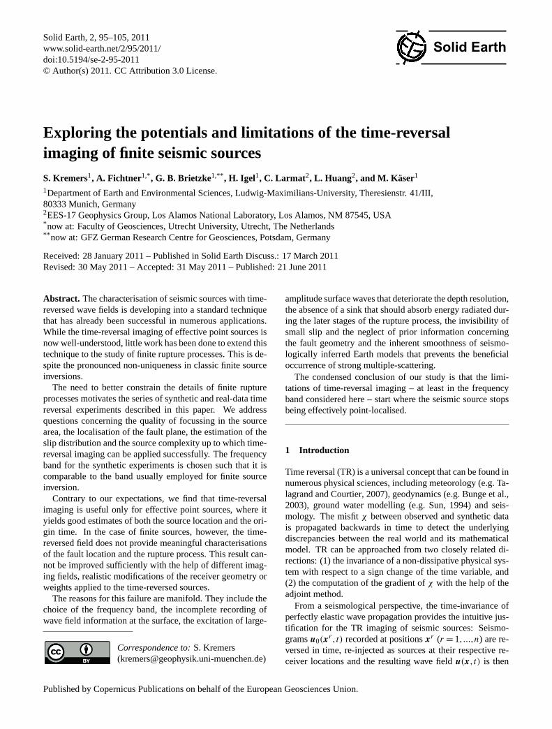
The model used in our synthetic tests is 160×170×40 kmwide. It comprises 60×60×16 elements, which correspondsto ∼ 3 million grid points when the polynomial degree is 4.This setup allows us to model wave fields with frequencies upto 2 Hz. Both the receiver configuration (Fig.1, left) and thestructural model (Fig.1, right) in most of our simulations arethe same as in the SPICE source inversion benchmark (Maiet al., 2007) that was intended to mimic the circumstancesof the 2000 Tottori (Japan) earthquake. For the real dataexperiment, we use the Japanese KiK-net stations (Fig.11)and the layered velocity model ofSemmane(2005). As weintend to work in the frequency range of kinematic sourceinversions (f = 0.1− 1 Hz) the velocity models were cho-sen alike. Even if the models seem dramatically smooth fortime-reversal purposes, we argue that no unknown complex-ity should be added.

To generate the time-reversed wave field, the displacementis recorded at the surface receivers, flipped in time and thenre-injected as three-component adjoint sources. For the prop-agation of the reverse field we use the same algorithm, setupand velocity model as for the forward simulation.

Solid Earth, 2, 95–105, 2011 www.solid-earth.net/2/95/2011/

S. Kremers et al.: Exploring the potentials and limitations of the time-reversal imaging of finite seismic sources 97

Fig. 1. Left: Geographic model setup. Stations are marked by trian-gles. The red line and the star mark the fault trace and the epicentrefor the finite-fault simulations in Sect.4. Right: Velocity and den-sity model used in all synthetic simulations.

3 Synthetic points source simulations

3.1 Single point source

Our first series of tests with one single double couple pointsource is deliberately simplistic. It is intended to serve asa reference for TR under near-ideal conditions. The TRmethod should be able to recover the point source, becauseotherwise there would be little hope for success in finite-source imaging.

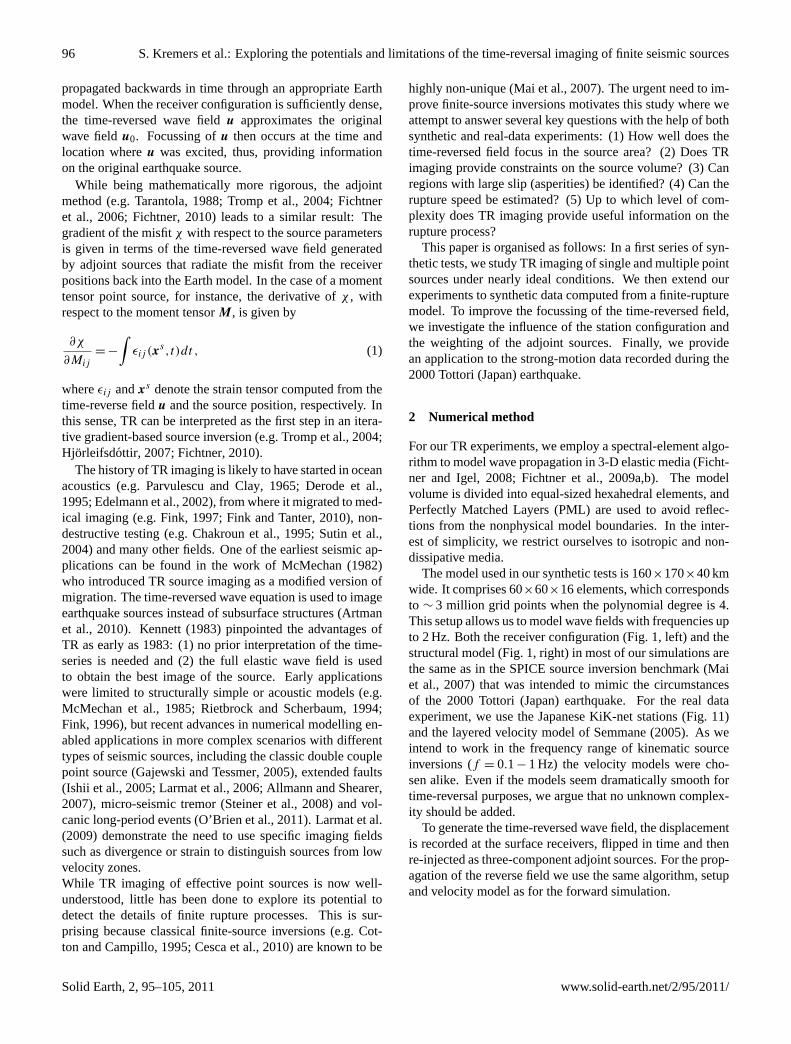
The moment tensor point-source, with onlyMxy differentfrom zero, is at 12.5 km depth. As source time function, weuse a Gaussian wavelet with a dominant frequency of 1 Hz.The wave field is computed for the 33 receivers shown in theleft panel of Fig.1. To illustrate the characteristics of thewaveforms, a selection of N–S-component synthetic seismo-grams is shown in Fig.2.

As suggested by Eq. (1), we monitor the time-reversedstrain componentεxy . Snapshots ofεxy at different timesare shown at the point-source depth (12.5 km) in Fig.3. Theadjoint field starts to propagate from the stations with thelargest epicentral distance and then focusses at the hypocen-tre ast approaches 0. Weaker or no focussing was observedfor the other components of the strain tensor, as expected.While the focussing ofεxy near the source can clearly beobserved,εxy |t=0 is still significantly different from zero inother regions of the model volume that are distant from thesource. These “ghost waves” result from the imperfect re-construction of the forward wave field by a finite number ofirregularly spaced adjoint sources located at the surface. De-pending on the particular setup, ghost waves may dominatethe reverse field, thus, masking the focussing at the sourcelocation.

Fig. 2. N–S-component synthetic seismograms recorded at the 33stations for a moment tensor point source with onlyMxy 6= 0. Thestations are sorted by distance to the epicentre and the traces arescaled to the maximum amplitude.

The influence of ghost waves can be reduced by using, forinstance, the energyE =

12v2 to image the source (Fig.3,

lower right). This leads to the suppression of contributionsfar from the source, but also to a less optimal focussing di-rectly at the source location. In numerous experiments, asimilar trade-off could be observed for other functionals ofthe time-reversed field, including the different components ofthe rotation vector∇ ×u and the rotation energy12(∇ ×u)2.This suggests that time-reversal imaging always involves acompromise between the focussing at the source and the sup-pression of ghost waves.

Our test with a point source moment tensor demonstratesthat focussing in space and time can indeed be observed, atleast under the previously described circumstances. This re-sult motivates the study of more complex scenarios. In thefollowing, we focus our attention on thexy-component ofthe time-reversed strain field,εxy . This restriction effectivelycorresponds to the injection of the prior information that thedisplacement on the infinitesimal or finite faults is a purestrike-slip.

3.2 Multiple point sources

Based on the encouraging results from the previous section,we add complexity to the source model and now considerthree double couple point sources (onlyMxy 6= 0) that arepositioned along the fault of the SPICE Tottori benchmark(Fig.1, left). The point sources have different initiation times

www.solid-earth.net/2/95/2011/ Solid Earth, 2, 95–105, 2011

98 S. Kremers et al.: Exploring the potentials and limitations of the time-reversal imaging of finite seismic sources

Fig. 3. Snapshots at the point-source depth (12.5 km) of the time-reversed strain fieldεxy at different times, and the energy12v2

(lower right) att = 0.

Fig. 4. Snapshots of the time-reversed strain fieldεxy at 12.5 kmdepth. Receiver and source locations are indicated by+ and◦, re-spectively. Focussing at all three source locations can be observedwith an uncertainty of∼ 5 km in space and∼ 1 s in time. The ob-served hypothetical rupture velocity is 2±0.3 km s−1, compared to2 km s−1 used to generate the forward wave field.

Fig. 5. Left: Time evolution of the normalisedSV =∫V ε2

xy d3xfor the single point source experiment from section3.1. A pro-nounced peak occurs at the focal timet = 0.0 s. Right: The sameas to the left, but for the multiple point source experiment fromSect.3.2. Peaks can be observed at the focal times of the differentpoint sources.

that correspond to a hypothetical rupture velocity of 2 km s−1

along the fault. The objective of this test is to reveal whethereach of the three point sources can be resolved individuallyin both time and space.

Snapshots of thexy-component reverse strain,εxy , areshown in Fig.4. Circles mark the point source locations.Moving from the upper left to the lower right corner, we ob-serve focussing at each of the three source locations aroundtheir respective initiation times of 16.9 s, 4.1 s and 0.0 s, withan uncertainty of∼ 1 s. The width of the regions wherefocussing can be observed is∼ 5 km, which is close tothe wavelength of the surface waves (∼ 3 km). From thiswe infer that the observed hypothetical rupture velocity is2±0.3 kms−1. We have, thus, obtained a first, and probablyoptimistic, estimate of the achievable space-time resolutionin the subsequent finite-source imaging experiments.

3.3 Quantitative assessment of focussing forpoint sources

So far, a purely visual analysis of the time-reversed wavefields was sufficient to observe focussing. However, in an-ticipation of more complex finite-source scenarios, we ex-amine the usefulness of a more quantitative criterion forthe focal time within a pre-defined test volume: startingwith the point source simulations we determine the quantitySV =

∫V

ε2xy d3x within a test volumeV around the source

locations, and then consider the time when the maximum oc-curs as an estimate of the focal time. Since the wavelengthsrange between 4 and 20 km, we letV extend 10 km in all di-rections around the hypocentre location. As we seek a quan-titative comparison of the focussing for various setups, wenormaliseSV by S⊗ =

∫⊗

ε2xy d3x, where⊗ denotes the re-

maining model volume outsideV .

Figure5 shows the normalisedSV for the single and multiplepoint source scenarios from Sects.3.1 and3.2, respectively.

Solid Earth, 2, 95–105, 2011 www.solid-earth.net/2/95/2011/

S. Kremers et al.: Exploring the potentials and limitations of the time-reversal imaging of finite seismic sources 99

Fig. 6. Synthetic slip (top) and rupture time (bottom) distributionsof the SPICE Tottori benchmark (Mai et al., 2007). Both the rupturespeed and the rise time are constant atvr = 2.7 km s−1 and 0.8 s,respectively.

Distinct peaks at the expected source times are clearly visiblein both cases. In the multiple point source experiment, weobserve that the peaks for the first two sources (at 0.0 s and4.1 s) are comparatively low, probably due to their spatialproximity and overlapping test volumes.

We conclude that the analysis ofSV is, at least for pointsources, a useful diagnostic that allows us to estimate focaltimes and to compare the quality of focussing for differentexperimental setups.

Considering the multiple point source test successful, wenow increase the complexity and make the transition to finitesource models.

4 Synthetic finite source simulations

The SPICE kinematic source inversion blind test offers theopportunity to analyse the performance of TR finite sourceimaging. The blind test mimics the 2000 Tottori (Japan)earthquake that was recorded by a large number of strong-motion sensors. Figure1 (left) shows the receiver configu-ration, the fault trace and the epicentre location. Syntheticseismograms for the 33 receivers are part of the benchmarkpackage. They were generated by pure strike slip motion andwith the slip and rupture time distributions shown in Fig.6.The excited wave field has a maximum frequency of 3 Hz.

Snapshots of the corresponding time-reversed strain com-ponentεxy are shown in the top panel of Fig.4. In reversetime, the rupture propagates in NW–SE direction. However,a clear focus restricted to the fault plane cannot be observed– in contrast to our expectation. The wave field remains dif-fuse, compared to the previous point source simulations. Arobust inference concerning the hypocentre location and theinitiation time is not possible.

Fig. 7. Top: Snapshots of the time-reversed strain componentεxy

at 12.5 km depth. The fault trace is indicated by the black line. Allsnapshots are shown in the same amplitude range. Bottom: Cumu-lative squared strainST =

∫T ε2

xy dt plotted on the fault plane (left)and integrated over depth (right).

In an attempt to facilitate the visual identification of boththe fault and the rupture process, we analyse the cumulativesquared strainST =

∫Tε2xy dt . Based on physical intuition

one would expectST to be large only in those regions wheresignificant strain occurs consistently over a longer period oftime, i.e., along the fault. However, neitherST directly on thefault plane norST integrated over depth allow any meaning-ful inference concerning the location of the fault or the origi-nal slip distribution (see the bottom panels of Fig.4). In fact,ST is largest near the surface, which reflects the dominanceof surface waves in the time-reversed wave field. Moreover,ST on the fault plane reaches a local maximum where theoriginal slip distribution (Fig.6) is close to zero. The depth-integratedST is largest far off the fault trace.

www.solid-earth.net/2/95/2011/ Solid Earth, 2, 95–105, 2011

100 S. Kremers et al.: Exploring the potentials and limitations of the time-reversal imaging of finite seismic sources

Similar efforts to enhance the focussing on the fault byintegrating, for instance,εxy or 1

2v2 over time, did not leadto any significant improvements. We are, therefore, led tothe early conclusion that no obvious functional of the time-reversed field allows us to identify the fault plane or the slipdistribution unambiguously. In what follows, we try to im-prove our results by (1) modifying the station distribution,and (2) weighting the adjoint sources.

4.1 Modifications of the station distribution

4.1.1 Dense regular grid of stations

The results from the previous section suggest that the numberof stations and their spatial distribution provided insufficientinformation for the reconstruction of the original wave field.This motivates a synthetic test with a larger number of re-ceivers (225 instead of 33) that are regularly spaced. Whilethis scenario may be too optimistic in the near future, it pro-vides valuable insight into TR finite source imaging underidealistic conditions.

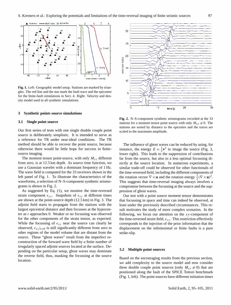
For this experiment, we computed synthetic seismogramswith the help of a Discontinuous Galerkin method (Kaserand Dumbser, 2006) that allows us to model the discontinu-ous displacement on the fault with high accuracy. Snapshotsof the resulting time-reversed strain componentεxy are dis-played in Fig.8.

Compared to Fig.4 (original station distribution), we ob-serve a sharper peak. Most of the energy propagates alongthe fault plane and in a direction that is consistent with therupture time distribution (6, bottom). However, the focus isstill elongated perpendicular to the fault, which complicatesits unambiguous identification. Any inference on the detailsof the original slip distribution (Fig.6) remains clearly im-possible.

To obtain more useful results, we again explored a varietyof functionals of the time-reversed field, including the time-integrated strain, the kinetic energy and the rotation ampli-tude. Neither of these functionals provided significant im-provements, thus, confirming our earlier conclusion that theoverall quality of the focussing is rather independent of thefield used for imaging.

4.2 Station arrays

As an alternative to the previous densification of the receiverconfiguration, we investigate the installation of several smallsub-arrays that are composed of four stations that form a2 km by 2 km quadrangle. This geometry is intended to havea beam-forming effect that hopefully improves the focussingof the time-reversed field.

The corresponding time-reversed strain fieldεxy is shownin Fig.9. The use of small sub-arrays clearly results in a morepronounced concentration of energy along the fault than with

Fig. 8. Snapshots of the time-reversed strain componentεxy at12.5 km depth for the dense array of 225 regularly spaced receivers.The fault trace is indicated by the black line. All snapshots areshown in the same amplitude range.

the original station setup (Figs.1 and4). However, the prob-lem of unambiguously identifying the fault itself remains un-resolved also with this configuration. Again, the use of var-ious functionals of the time-reversed field does not lead tosignificantly better results.

The previous experiments seem to imply that modifica-tions of the receiver geometry are unlikely to improve thereconstruction of the original wave field to an extent that issufficient to infer the slip distribution on the fault or even thefault itself.

4.3 Weighting of adjoint sources

A visual analysis of this failure (see Figs.4 and9) revealsthat the highly unequal contributions from different receiversmay be part of the problem. While receivers close to the faultdominate the time-reversed field due to the high amplitudesof the recorded waveforms, receivers at larger distances makeonly negligible contributions. This suggests that the recon-struction of the original wave field may be improved by as-signing weights to the adjoint sources at positionxr that com-pensate for the geometric amplitude reduction with increas-ing propagation distance. In the following, we examine theeffects of two different schemes where the weights are pro-portional to (1) the squared epicentral distance, and (2) theinverse energy of the recorded waveforms, i.e., 2/

∫v(xr)2dt .

It is important to note that the weighting scheme based on thedistance from the epicentre corresponds to the incorporation

Solid Earth, 2, 95–105, 2011 www.solid-earth.net/2/95/2011/

S. Kremers et al.: Exploring the potentials and limitations of the time-reversal imaging of finite seismic sources 101

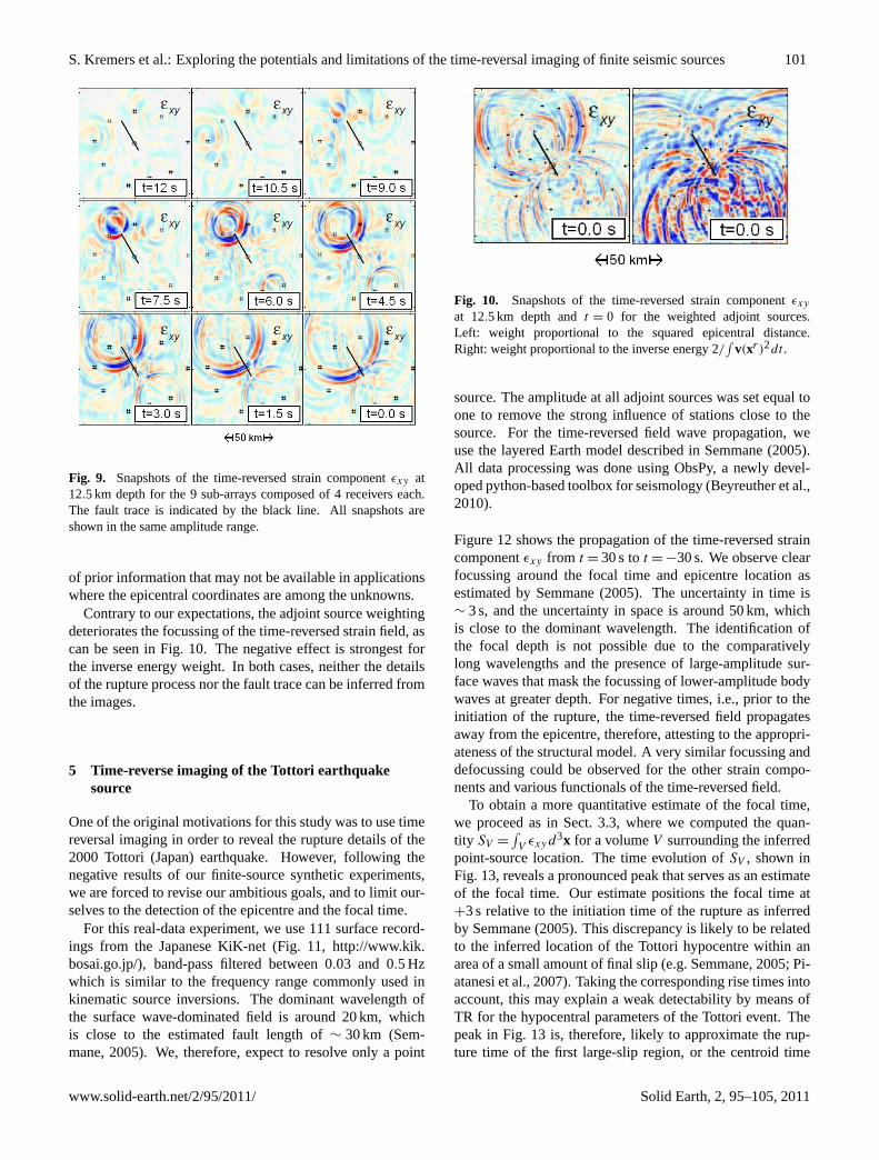
Fig. 9. Snapshots of the time-reversed strain componentεxy at12.5 km depth for the 9 sub-arrays composed of 4 receivers each.The fault trace is indicated by the black line. All snapshots areshown in the same amplitude range.

of prior information that may not be available in applicationswhere the epicentral coordinates are among the unknowns.

Contrary to our expectations, the adjoint source weightingdeteriorates the focussing of the time-reversed strain field, ascan be seen in Fig.10. The negative effect is strongest forthe inverse energy weight. In both cases, neither the detailsof the rupture process nor the fault trace can be inferred fromthe images.

5 Time-reverse imaging of the Tottori earthquakesource

One of the original motivations for this study was to use timereversal imaging in order to reveal the rupture details of the2000 Tottori (Japan) earthquake. However, following thenegative results of our finite-source synthetic experiments,we are forced to revise our ambitious goals, and to limit our-selves to the detection of the epicentre and the focal time.

For this real-data experiment, we use 111 surface record-ings from the Japanese KiK-net (Fig.11, http://www.kik.bosai.go.jp/), band-pass filtered between 0.03 and 0.5 Hzwhich is similar to the frequency range commonly used inkinematic source inversions. The dominant wavelength ofthe surface wave-dominated field is around 20 km, whichis close to the estimated fault length of∼ 30 km (Sem-mane, 2005). We, therefore, expect to resolve only a point

Fig. 10. Snapshots of the time-reversed strain componentεxy

at 12.5 km depth andt = 0 for the weighted adjoint sources.Left: weight proportional to the squared epicentral distance.Right: weight proportional to the inverse energy 2/

∫v(xr )2dt .

source. The amplitude at all adjoint sources was set equal toone to remove the strong influence of stations close to thesource. For the time-reversed field wave propagation, weuse the layered Earth model described inSemmane(2005).All data processing was done using ObsPy, a newly devel-oped python-based toolbox for seismology (Beyreuther et al.,2010).

Figure12 shows the propagation of the time-reversed straincomponentεxy from t = 30 s tot = −30 s. We observe clearfocussing around the focal time and epicentre location asestimated bySemmane(2005). The uncertainty in time is∼ 3 s, and the uncertainty in space is around 50 km, whichis close to the dominant wavelength. The identification ofthe focal depth is not possible due to the comparativelylong wavelengths and the presence of large-amplitude sur-face waves that mask the focussing of lower-amplitude bodywaves at greater depth. For negative times, i.e., prior to theinitiation of the rupture, the time-reversed field propagatesaway from the epicentre, therefore, attesting to the appropri-ateness of the structural model. A very similar focussing anddefocussing could be observed for the other strain compo-nents and various functionals of the time-reversed field.

To obtain a more quantitative estimate of the focal time,we proceed as in Sect.3.3, where we computed the quan-tity SV =

∫V

εxy d3x for a volumeV surrounding the inferredpoint-source location. The time evolution ofSV , shown inFig. 13, reveals a pronounced peak that serves as an estimateof the focal time. Our estimate positions the focal time at+3 s relative to the initiation time of the rupture as inferredby Semmane(2005). This discrepancy is likely to be relatedto the inferred location of the Tottori hypocentre within anarea of a small amount of final slip (e.g.Semmane, 2005; Pi-atanesi et al., 2007). Taking the corresponding rise times intoaccount, this may explain a weak detectability by means ofTR for the hypocentral parameters of the Tottori event. Thepeak in Fig.13 is, therefore, likely to approximate the rup-ture time of the first large-slip region, or the centroid time

www.solid-earth.net/2/95/2011/ Solid Earth, 2, 95–105, 2011

102 S. Kremers et al.: Exploring the potentials and limitations of the time-reversal imaging of finite seismic sources

131

o E

132

o E

133

o E

134

o E

135

o E

136

o E

33oN

30’

34oN

30’

35oN

30’

36oN

eastern longitude

nort

hern

latit

ude

Fig. 11. Source-receiver geometry of the real-data TR experimentfor the 2000 Tottori earthquake. Red triangles mark the positions ofthe 111 stations used in the experiment, and the black star indicatesthe epicentre as inferred bySemmane(2005). The seismogramsshown are vertical component velocities in the chosen frequencyband.

Fig. 12.Snapshots of the time-reversed strain componentεxy at thesurface for the Tottori data recorded at the 111 stations shown inFig. 11. The coastlines are omitted to enhance the visibility of thetime-reversed field. Estimates of both the focal time (t = 0 s) andthe epicentre location (black dot) are taken fromSemmane(2005).

of the whole event (both at about+4 s, according toSem-mane(2005) or Piatanesi et al.(2007) rather than the preciseinitiation time of the finite-size rupture.

Fig. 13. Time evolution of the normalisedSV =∫V ε2

xy d3x for avolumeV that extends 20 km by 20 km around the epicentre as es-timated from the time-reversal images from Fig.12. The peak oc-curs at+3 s relative to the focal time estimated bySemmane(2005)(t = 0).

6 Discussion

In the previous sections, we explored the potentials and lim-itations of the TR imaging of seismic sources on regionalscales. For this we studied a variety of scenarios with bothsynthetic and real data.

The potential of the method clearly lies in the estimationof the location and the timing of point sources. In a series ofsynthetic experiments, we were able to observe the focussingof the time-reversed field in the vicinity of the original pointsource location and the original focal time. The uncertaintiesin the source location and time are governed by the frequencycontent and the receiver configuration. Our point source sce-narios provide a proof of principle, but they are idealistic inthe sense that we disregarded errors in the data and the as-sumed Earth model.

Our primary interest was in the detection of finite-ruptureprocesses. Unfortunately, however, neither the rupture de-tails nor the position of the fault itself could be inferredfrom the properties of the time-reversed wave field. To im-prove this result, we analysed various functionals of the wavefield (strain, energy, rotations), modified the receiver geome-try (densification, sub-arrays) and applied weights to the ad-joint sources in order to compensate for geometric spreading.None of these strategies can be considered successful.

The reasons for this failure are manifold:

1. Incomplete information: Firstly and most importantly,the information recorded at the surface is plainly insuf-ficient to reconstruct the original wave field with an ac-curacy that allows for the unambiguous identification ofthe rupture process. For instance, the body wave energyradiated downwards is entirely disregarded. This distin-guishes TR on regional scales from TR on global scaleswhere information is lost only through dissipation.

Solid Earth, 2, 95–105, 2011 www.solid-earth.net/2/95/2011/

S. Kremers et al.: Exploring the potentials and limitations of the time-reversal imaging of finite seismic sources 103

2. Large-amplitude surface waves: Partly as a conse-quence of the previous item, the time-reversed fieldfrom stations that are distant from the fault is dominatedby large-amplitude surface waves. The surface wavestend to mask the focussing of the lower-amplitude bodywaves that are primarily contributed by the stationscloser to the fault. This effect results in a weak depthresolution, which means, in particular, that the focaldepth can hardly be constrained.

3. The missing sink: An even more profound and generalreason for failure is the incompleteness of the TR pro-cedure. Our interest is in the seismic wave equation

ρ u(x,t)−∇ ·σ (x,t)= f (x,t) (2)

whereu, σ andf denote the seismic displacement field,the stress tensor and an external force density. A com-plete time reversal of equation2 would require the im-plementation of a sinkf (x,−t) that acts as the coun-terpart of the sourcef (x,t) in the forward direction,and that absorbs elastic energy so that the time-reversedfield is zero fort < 0. The sink, however, is disregardedsimply because it is unknown. The missing sink poses aserious problem for finite-source inversions when faultsegments are active at different times. The energy fromsegments that act late in the rupture process is not ab-sorbed by the sink and, therefore, continues to propa-gate. The unabsorbed energy masks the focussing at thefault segments that act early in the rupture process. Theimmediate implication is that TR for finite sources is al-ways dominated by those fault segments with large slipnear the end of the rupture time.

4. Invisibility of small slip: A corollary of the previ-ous item is that no information can be obtained aboutthe rupture details on segments of the fault with smallamount of final slip. This means, in particular, thatthe hypocentral parameters cannot be detected in thosecases where the rupture initiation is associated withsmall slip.

5. Lack of prior information: The poor performance ofTR finite-source imaging as compared to the classicalkinematic source inversions is also due to the neglectof an apparently essential piece of prior information:The rupture occurs along a fault and is not diffusely dis-tributed throughout the model volume.

6. Incomplete knowledge of the 3-D Earth structure:While excluded a priori in the synthetic experiments,inaccurate Earth models can prevent focussing in real-data applications. The focussing observed in our ex-periment with Tottori data suggests that the model issufficient to explain at least the arrival times of the di-rect waves. However, the absence of horizontal het-

erogeneities in the model does not allow for the cor-rect back-propagation of scattered or even multiple-scattered waves. This issue is closely related to

7. The insufficient complexity of 3-D Earth models thatresults either from the inherent smoothness of the Earthor the limited resolution of seismic tomography. Thepresence of strong multiple scattering is known to en-hance focussing in laboratory experiments, but cannotbe exploited in seismology where the knowledge aboutsub-wavelength heterogeneities is too inaccurate.

7 Conclusions

The principal conclusions to be drawn from our work areas follows: (1) Time-reversal imaging is well-suited to inferboth the location and the timing of point sources. (2) Time-reversal imaging in the used frequency range is not able todetect the details of finite rupture processes. Neither mod-ifications of the receiver configuration (within reasonablebounds) nor the weighting of adjoint sources lead to suffi-cient improvements. (3) The dominant causes for this failureare the incomplete recordings of wave field information atthe surface, the presence of large-amplitude surface wavesthat deteriorate the depth resolution, the missing sink thatshould absorb energy radiated during the later stages of therupture process, the invisibility of small slip and the neglectof prior information.

While our experiments are certainly not exhaustive, theynevertheless suggest that the limitations of TR imaging startwhere the source stops being point-localised.

Acknowledgements.HI and SK gratefully acknowledge supportthrough the Geophysics Group at Los Alamos National Labs fortheir research visits in 2008. We thank the Leibniz RechenzentrumMunich for providing access to their supercomputer facilities andthe IT support team (Jens Oeser) at the Geophysics Section ofthe Department of Earth Sciences at LMU Munich. We are alsograteful to Martin Mai for giving us access to the SPICE dataset.We are grateful to J.-P. Montagner and B. Artman whose commentsimproved the manuscript. This work would not have been possiblewithout the support of the European Commission in connectionwith the Research and Training Network SPICE (spice-rtn.org) andthe Initial Training Network QUEST (quest-itn.org).

Edited by: R. Carbonell

www.solid-earth.net/2/95/2011/ Solid Earth, 2, 95–105, 2011

104 S. Kremers et al.: Exploring the potentials and limitations of the time-reversal imaging of finite seismic sources

References

Allmann, B. P. and Shearer, P. M.: A high-frequency secondaryevent during the 2004 Parkfield earthquake., Science (New York,N.Y.), 318, 1279–83,doi:10.1126/science.1146537, http://www.ncbi.nlm.nih.gov/pubmed/18033878, 2007.

Artman, B., Podladtchikov, I., and Witten, B.: Source locationusing time-reverse imaging, Geophys. Prospect., 58, 861–873,doi:10.1111/j.1365-2478.2010.00911.x, 2010.

Beyreuther, M., Barsch, R., Krischer, L., Megies, T., Behr, Y., andWassermann, J.: ObsPy: A Python Toolbox for Seismology,Seismol. Res. Lett., 81, 530–533,doi:10.1785/gssrl.81.3.530,2010.

Bunge, H.-P., Hagelberg, C. R., and Travis, B. J.: Mantle circulationmodels with variational data assimilation: inferring past mantleflow and structure from plate motion histories and seismic to-mography, Geophys. J. Int., 152, 280–301,doi:10.1046/j.1365-246X.2003.01823.x, 2003.

Cesca, S., Heimann, S., Stammler, K., and Dahm, T.: Au-tomated procedure for point and kinematic source inver-sion at regional distances, J. Geophys. Res., 115, B06304,doi:10.1029/2009JB006450, 2010.

Chakroun, N., Fink, M., and Wu, F.: Time reversal processing inultrasonic nondestructive testing, IEEE T. Ultrason. Ferr., 42,1087–1098,doi:10.1109/58.476552, 1995.

Cotton, F. and Campillo, M.: Frequency domain inversion of strongmotions: Application to the 1992 Landers earthquake, J. Geo-phys. Res., 100, 3961–3975, 1995.

Derode, A., Roux, P., and Fink, M.: Robust Acoustic Time Reversalwith High-Order Multiple Scattering, Phys. Rev. Lett., 75, 4206–4209,doi:10.1103/PhysRevLett.75.4206, 1995.

Edelmann, G., Akal, T., Hodgkiss, W., and Kuperman, W.: An ini-tial demonstration of underwater acoustic communication usingtime reversal, IEEE Journal of Oceanic Engineering, 27, 602–609,doi:10.1109/JOE.2002.1040942, 2002.

Fichtner, A.: Full seismic waveform modelling and inversion,Springer, Heidelberg, 2010.

Fichtner, A. and Igel, H.: Efficient numerical surface wave prop-agation through the optimization of discrete crustal models-a technique based on non-linear dispersion curve matching(DCM), Geophys. J. Int., 173, 519–533,doi:10.1111/j.1365-246X.2008.03746.x, 2008.

Fichtner, A., Bunge, H., and Igel, H.: The adjoint method inseismologyI. Theory, Phys. Earth Planet. In., 157, 86–104,doi:10.1016/j.pepi.2006.03.016, 2006.

Fichtner, A., Igel, H., Bunge, H.-P., and Kennett, B. L. N.: Simu-lation and Inversion of Seismic Wave Propagation on Continen-tal Scales Based on a Spectral-Element Method, Journal of Nu-merical Analysis, Industrial and Applied Mathematics, 4, 11–22,2009a.

Fichtner, A., Kennett, B. L. N., Igel, H., and Bunge, H.-P.: Fullseismic waveform tomography for upper-mantle structure in theAustralasian region using adjoint methods, Geophys. J. Int., 179,1703–1725,doi:10.1111/j.1365-246X.2009.04368.x, 2009b.

Fink, M.: Time reversal in acoustics, Contemp. Phys., 37, 95–109,1996.

Fink, M.: Time reversed acoustics, Phys. Today, 50, 34–40, 1997.Fink, M. and Tanter, M.: Multiwave imaging and super resolution,

Physics Today, 63, 28–33, 2010.

Gajewski, D. and Tessmer, E.: Reverse modelling for seis-mic event characterization, Geophys. J. Int., 163, 276–284doi:10.1111/j.1365–246X.2005.02,732.x, 2005.

Hjorleifsdottir, V.: Earthquake source characterization using 3DNumerical Modeling, Ph.D. thesis, California Institute of Tech-nology, Pasadena, California, USA, 2007.

Ishii, M., Shearer, P. M., Houston, H., and Vidale, J. E.: Ex-tent, duration and speed of the 2004 Sumatra-Andaman earth-quake imaged by the Hi-Net array., Nature, 435, 933–6,doi:10.1038/nature03675, 2005.

Kaser, M. and Dumbser, M.: An arbitrary high-order discontinu-ous Galerkin method for elastic waves on unstructured meshes– I. The two-dimensional isotropic case with external sourceterms, Geophys. J. Int., 166(2), 855–877,doi:10.1111/j.1365–246X.2006.03,051.x, 2006.

Kennett, B. L. N.: A new way to estimate seismic source parame-ters, Nature,f 302, 659–660, 1983.

Larmat, C., Montagner, J.-P., Fink, M., Capdeville, Y., Tourin, A.,and Clevede, E.: Time-reversal imaging of seismic sources andapplication to the great Sumatra earthquake, Geophys. Res. Lett.,33, L19312,doi:10.1029/2006GL026336, 2006.

Larmat, C. S., Guyer, R. A., and Johnson, P. A.: Tremorsource location using time reversal: Selecting the appro-priate imaging field, Geophys. Res. Lett., 36, L22304,doi:10.1029/2009GL040099, 2009.

Mai, P., Burjanek, J., Delouis, B., Festa, G., Francois-Holden, C.,Monelli, D., Uchide, T., and Zahradnik, J.: Earthquake SourceInversion Blindtest: Initial Results and Further Developments,AGU Fall Meeting San Francisco, 2007.

McMechan, G. A.: Determination of source parameters by wave-field extrapolation, Geophys. J. R. astr. SOC., 71, 613–628,doi:10.1111/j.1365-246X.1982.tb02788.x, 1982.

McMechan, G. A., Luetgert, J. H., and Mooney, W. D.: Imagingof earthquake sources in Long Valley Caldera, California, 1983,Bull. Seismol. Soc. Am., 75, 1005–1020, 1985.

O’Brien, G. S., Lokmer, I., De Barros, L., Bean, C. J., Saccorotti,G., Metaxian, J.-P., and Patane, D.: Time reverse location of seis-mic long-period events recorded on Mt Etna, Geophys. J. Int.,184, 452–462,doi:10.1111/j.1365-246X.2010.04851.x, 2011.

Parvulescu, A. and Clay, C. S.: Reproducibility of signal trans-missions in the ocean, Radio Electron. Eng., 29, 223–228,doi:10.1049/ree.1965.0047, 1965.

Piatanesi, A., Cirella, A., Spudich, P., and Cocco, M.: A globalsearch inversion for earthquake kinematic rupture history: Appli-cation to the 2000 western Tottori, Japan earthquake, J. Geophys.Res., 112, B07314,doi:10.1029/2006JB004821, 2007.

Rietbrock, A. and Scherbaum, F.: Acoustic imaging of earth-quake sources from the Chalfant Valley, 1986, aftershockseries, Geophys. J. Int., 119, 260–268,doi:10.1111/j.1365-246X.1994.tb00926.x, 1994.

Semmane, F.: The 2000 Tottori earthquake: A shallow earthquakewith no surface rupture and slip properties controlled by depth, J.Geophys. Res., 110, B03306,doi:10.1029/2004JB003194, 2005.

Steiner, B., Saenger, E. H., and Schmalholz, S. M.: Time-reverse modeling of microtremors: Application to hydrocar-bon reservoir localization, Geophys. Res. Lett., 35, L03307,doi:10.1029/2007GL032097, 2008.

Sun, N.-Z.: Inverse problems in ground water modelling, KluwerAcademic Publishers, 1994.

Solid Earth, 2, 95–105, 2011 www.solid-earth.net/2/95/2011/

S. Kremers et al.: Exploring the potentials and limitations of the time-reversal imaging of finite seismic sources 105

Sutin, A. M., TenCate, J. A., and Johnson, P. A.: Single-channeltime reversal in elastic solids, The Journal of the Acoustical So-ciety of America, 116, 2779,doi:10.1121/1.1802676, 2004.

Talagrand, O. and Courtier, P.: Variational Assimilation of Me-teorological Observations With the Adjoint Vorticity Equa-tion. I: Theory, Q. J. Roy. Meteor. Soc., 113, 1311–1328,doi:10.1002/qj.49711347812, 2007.

Tarantola, A.: Theoretical background for the inversion of seismicwaveforms including elasticity and attenuation, Pure Appl. Geo-phys., 128, 365–399,doi:10.1007/BF01772605, 1988.

Tromp, J., Tape, C., and Liu, Q.: Seismic tomography, adjoint meth-ods, time reversal and banana-doughnut kernels, Geophys. J. Int.,160, 195–216,doi:10.1111/j.1365-246X.2004.02453.x, 2004.

www.solid-earth.net/2/95/2011/ Solid Earth, 2, 95–105, 2011