1

Exploring the Possibility of New Physics

Part I:

Quantum Mechanics and the Warping of

Spacetime

Julian Williams February 2017 jjawilliams@xtra.co.nz

Abstract

This paper suggests new physics. In a completely different approach, it proposes fundamental

particles formed from infinite superpositions with mass borrowed from a Higgs type scalar

field. However energy is also borrowed from zero point vector fields. Just as the Standard

Model divides the fundamental particles into two types…those with mass and those without,

the Higgs mechanism providing the difference…infinite superpositions seem also to divide

naturally into two sets: (a) those with “infinitesimal” mass, and (b) those with significant

mass (from micro electron volts upwards). In the infinitesimal set (a), photons, gluons and

gravitons (to fit with cosmology and the expansion of the cosmos) all have 3310

eV mass,

approximately the inverse of the causally connected horizon radius. These values are so close

to zero the symmetry breaking of the Standard Model remains essentially valid. These

particles travel so close to the speed of light they have virtually fixed helicity, with the Higgs

mechanism increasing their mass from infinitesimal type (a) to significant or measureable

type (b) values. Also the energy in the zero point fields (borrowed to build the fundamental

particles) is limited, particularly at the extreme wavelengths of virtual gravitons interacting at

near horizon radii. Any causally connected region grows with time after the big bang and the

number of virtual gravitons with wavelengths similar to the size of the causally connected

region increases approximately as the square of the causally connected mass. Space has to

expand exponentially with time in an accelerating manner after the big bang to make

available the zero point energy to meet this increased requirement. For similar reasons the

extra gravitons near mass concentrations change the metric in proportion to 2 /m r , in

accordance with the Schwarzschild solution of Einstein’s equations. There is a maximum

wavelength virtual graviton probability density min min minGk GkK dk where minGk

K is an

invariant scalar, in any coordinates, at all points in spacetime. But the local value of the

corresponding minimum wavenumber 1

min Horizonk R

depends on, both the cosmic time T, and

the value of 00g in the local metric. Approximately the first two thirds of this paper look at

building and analysing the fundamental particles formed from infinite virtual superpositions.

The final portion looks at the expanding Universe and possible connections with General

Relativity; but only after attempting to show that infinite superpositions can be equivalent to

the Standard Model fundamental particles, apart from infinitesimal differences.

2

1 Introduction ........................................................................................................................ 4

1.1 Summary ..................................................................................................................... 4

1.1.1 General Relativity as our starting point ............................................................... 4

1.1.2 Primary interactions and Secondary interactions ................................................. 6

1.1.3 Photons, gluons and gravitons with infinitesimal mass ( 3310 eV

). .................. 7

1.1.4 Superpositions require only squared vector potentials ........................................ 8

2 Building Infinite Virtual Superpositions .......................................................................... 11

2.1 The possibility of Infinite Superpositions ................................................................. 11

2.1.1 Early ideas .......................................................................................................... 11

2.1.2 Dividing probabilities into the product of two component parts ....................... 12

2.2 Spin Zero Virtual Preons from a Higgs type Scalar Field......................................... 13

2.2.1 Groups of eight preons that form superpositions ............................................... 13

2.2.2 Primary coupling constants behave differently and actually are constant ......... 15

2.2.3 Primary interactions also behave differently ..................................................... 16

2.3 Virtual Wavefunctions that form Infinite Superpositions ......................................... 18

2.3.1 Infinite families of similar virtual wavefunctions .............................................. 18

2.3.2 Eigenvalues of these virtual wavefunctions and parallel momentum vectors ... 19

3 Properties of Infinite Superpositions ............................................................................... 21

3.1 What is the Amplitude that nk is in an m state? ..................................................... 21

3.1.1 Four vector transformations ............................................................................... 21

3.1.2 Feynman diagrams of primary interactions ....................................................... 23

3.1.3 Different ways to express superpositions .......................................................... 26

3.2 Mass and Total Angular Momentum of Infinite Superpositions............................... 28

3.2.1 Total mass of massive infinite superpositions ................................................... 28

3.2.2 Angular momentum of massive infinite superpositions .................................... 29

3.2.3 Mass and angular momentum of multiple integer n superpositions .................. 30

3.3 Ratios between Primary and Secondary Coupling .................................................... 31

3.3.1 Initial simplifying assumptions .......................................................................... 31

3.3.2 Restrictions on possible Eigenvalue changes .................................................... 34

3.3.3 Looking at just one vertex of the interaction first .............................................. 35

3.3.4 Assumptions when looking at both vertexes of the interaction ......................... 37

3.4 Electrostatic Energy between two Infinite Superpositions ....................................... 40

3.4.1 Using a simple quantum mechanics early QED approach ................................. 40

3.5 Magnetic Energy between two spin aligned Infinite Superpositions ........................ 45

3.5.1 Amplitudes of transversely polarized virtual emmited photons ........................ 47

3.5.2 Checking our normalization factors ................................................................... 48

4 High Energy Superposition Cutoffs ................................................................................. 51

4.1 Electromagnetic Coupling to Spin ½ Infinite Superpositions ................................... 51

4.1.1 Comparing this with the Standard Model .......................................................... 53

4.2 Introducing Gravity into our Equations .................................................................... 55

4.2.1 Simple square superposition cutoffs .............................................................. 55

4.2.2 All N = 1 superpositions cutoff at Planck Energy but interactions at less ......... 58

3

4.3 Solving for spin ½, spin 1 and spin 2 superpositions ................................................ 60

5 The Expanding Universe and General Relativity ............................................................ 61

5.1 Zero point energy densities are limited ..................................................................... 61

5.1.1 Virtual Particles and Infinite Superpositions ..................................................... 62

5.1.2 Virtual graviton density at wavenumber k in a causally connected Universe .. 62

5.2 Can we relate all this to General Relativity? ............................................................. 65

5.2.1 Approximations with possibly important consequences.................................... 65

5.2.2 The Schwarzchild metric near large masses ...................................................... 69

5.3 The Expanding Universe ........................................................................................... 71

5.3.1 Holographic horizons and red shifted Planck scale zero point modes............... 72

5.3.2 Plotting available and required zero point quanta.............................................. 74

5.3.3 Possible consequences of a small gravitational coupling constant. ................... 76

5.3.4 A possible exponential expansion solution and scale factors ............................ 76

5.3.5 Possible values for b and plotting scale factors ................................................. 79

5.3.6 An infinitesimal change to General Relativity effective at Cosmic scale ......... 79

5.3.7 Non comoving coordinates in Minkowski spacetime where g . .......... 80

5.3.8 Non comoving coordinates when g . .................................................... 81

5.3.9 Is Inflation really necessary in this proposed scenario? ..................................... 83

6 Further consequences of Infinite Superpositions ............................................................. 84

6.1 Low frequency Infinite Superposition cutoffs .......................................................... 84

6.1.1 Quantifying the approximate effect of min0k on infinite superpositions ....... 84

6.2 Infinitesimal Masses and N = 2 Superpositions ........................................................ 84

6.2.1 Cutoff behaviours for N = 1 & N = 2 superpositions ......................................... 86

6.2.2 Virtual particle pairs emerging from the vacuum and space curvature ............. 87

6.2.3 Redshifted zero point energy from the horizon behaves differently to local ..... 88

6.2.4 Revisiting the building of infinite superpositions .............................................. 88

6.2.5 The primary to secondary graviton coupling ratio G ...................................... 89

6.2.6 N=1 & N=2 Bosons and the Higg’s mechanism ............................................... 90

6.3 Black Holes, the Firewall Paradox and possible Spacetime Boundaries .................. 90

6.4 Dark Matter possibilities ........................................................................................... 90

6.5 Higgs Boson .............................................................................................................. 90

6.6 Constancy of fundamental charge ............................................................................. 90

6.7 Feynman’s Strings ..................................................................................................... 91

7 Conclusions ...................................................................................................................... 91

8 Addendum ........................................................................................................................ 93

References ................................................................................................................................ 93

4

1 Introduction

Many Physicists today (probably a large majority) are; Supersymmetry supporters, String

theory supporters, Inflation supporters, Metaverse supporters, etc. They will perhaps see the

ideas presented in this paper as irrelevant. On the other hand there is a much smaller, but

possibly growing band who are increasingly disillusioned at what seems to them to be a lack

of real, concrete or testable progress over the last 30 to 40 years or so since the development

of the brilliantly successful and accurate Standard Model. This smaller band adheres to the

tradition, started originally by the Greeks but more particularly over the last few centuries, of

empirically testable science: Newton’s theories, Maxwell’s equations, General Relativity,

Quantum mechanics and lastly the Standard Model representing the pinnacle of this testing

by experiment era. All these great theories were developed from experiments. As

instrumentation accuracy slowly improved, and experiments grew more refined, the above

theories, each accurate in their day, slowly evolved from one to the next. The current

situation in contrast, invites some important and relevant questions; for example:

1. Is Supersymmetry really the answer to the problems with the Standard Model?

2. Are the extra dimensions of String Theory really necessary?

3. Is “The Multiverse” the only explanation of accelerating cosmic expansion?

4. Is Inflation really necessary? And so on.

Approaching all this in a new direction, this paper explores possible solutions to these

questions in a completely different way; but still using very simple basic principles of

quantum mechanics and relativity. Apart from infinitesimal differences it is (almost)

consistent with the Standard Model. It requires the universe to expand exponentially after the

big bang in an accelerating manner that is testable. This is so regardless of the value of ,

with no need for Dark Energy. It changes the metric around mass concentrations in

accordance with an infinitesimally modified General Relativity. And it all only works if the

Universe is flat on average, with no need for inflation.

1.1 Summary

Papers modifying the Standard Model are too numerous to list, however we briefly touch on a

small number of some early versions of these in section 1.1.2. The approach in this paper is

very different from that in most of these earlier papers. The main differences are summarized

below.

1.1.1 General Relativity as our starting point

General Relativity tells us that all forms of mass, energy and pressure are sources of the

gravitational field. Thus to create gravitational fields all spin ½ leptons & quarks, spin 1

gluons, photons, 0W & Z

particles etc. emit virtual gravitons, except possibly gravitons

themselves (section 6.2.5), as gravitational energy is not part of the Einstein tensor.

5

The starting point of this paper assumes there is a common thread uniting these fundamental

particles making this possible. Equations are developed that unite the amplitudes of the

colour and electromagnetic coupling constants with that of gravity. The precision required by

quantum mechanics for half integral and integral angular momentum allows gravity to be

included, despite the vast disparity in magnitude between gravity and the other two. This

combination of colour, electromagnetic and gravitational amplitudes in the same equation is

possible because of a radically different approach taken in this paper: An approach using

infinite superpositions of positive and negative integral angular momentum virtual

wavefunctions for spin ½, spin 1 and spin 2 particles. The final result is almost identical to

the Standard Model, with infinitesimal but important differences.

The total angular momentum can be summed over all wavenumbers ;k from 0k to some

cutoff valuecutoff

k . We will assume (as with many unification theories) that the cutoff for

these infinite superpositions is somewhere near Planck scale. Firstly imagine a universe

where the gravitational constant 0G . As 0G , the Planck length 0P

L , the Planck

energy andP

E cutoff

k also. If we sum the angular momentum of these infinite

superpositions when 0G (i.e. from 0k to )cutoff

k we get precisely half integral or

integral for the fundamental spin ½, spin 1 & spin 2 particles in appropriate m states. If we

now put 0G the infinitesimal effect of including gravity can be balanced by an equal but

opposite effect due to the non-infinite cutoff value in .k A near Planck scale superposition

cutoff requires gravity to be included to get precisely half integral or integral . (Section 4.2)

These infinite superpositions have another very relevant property relating to the fact that all

experiments indicate that fundamental particles such as electrons behave as point particles.

Each wavefunction with wavenumber k , which we label as k , has a maximum radial

probability at 1/r k and they all look the same (Figure 1.1. 1.)

Figure 1.1. 1 The radial probability of the dominant 6n for spin ½ wavefunction 6k .

Every wavefunction k of these infinite superpositions, interacts only with virtual photons

(for example) of the same ;k if superpositions representing say an electron are probed with

such photons (that interact only with wavefunction k ) the resolution possible is of the same

4*R R

k

kr

6

order as the dimensions of ,k

both have 1/ .r k The higher the energy of the probing

particle the smaller the k

it interacts with, the resolution of an observing photon can never

be fine enough to see any k dimensions. Even if this energy approaches the Planck value,

with a matching k radius near the Planck length it is still not possible to resolve it. This

behaviour is consistent with the quantum mechanical properties of point particles.

1.1.2 Primary interactions and Secondary interactions

Supposing that superpositions can in fact build the fundamental spin ½, spin 1, and spin 2

particles, then what builds the superpositions? Before answering that question, this paper can

only make sense if we divide the world of all interactions into two categories.

Secondary Interactions are those we are familiar with, and are covered by the Standard

Model; but with the addition of gravity, which is not included in the Standard Model. They

take place between the fundamental spin ½, spin 1 and spin 2 particles formed from infinite

superpositions. They are the QED/QCD etc, interactions of all real world experiments.

Primary Interactions we conjecture on the other hand are those that build infinite

superpositions. They are virtual, and completely hidden to the real world of experiments.

The majority of this paper is about these primary interactions, and the superpositions they

build representing the fundamental spin ½, spin 1 and spin 2 particles. Primary interactions

are between spin zero particles borrowed from a Higgs type scalar field and the zero point

vector fields. In the 1970’s models were proposed with preons as common building blocks of

leptons and quarks [4] [5] [6] [7]. In contrast with the virtual particles in this paper some of

these earlier models used real spin ½ building blocks. Real substructure has difficulties with

large masses if compressed into the small volumes required to approach point particle

behaviour. On the other hand with virtual substructure borrowing energy from zero point

fields the mass contribution at high k values can be cancelled (section 3.2.1). As in earlier

models this paper also calls the common building blocks preons, but here the preons are both

virtual and spin zero. They also now build all spin ½ leptons and quarks, spin 1 gluons,

photons, W & Z particles, plus spin 2 gravitons in contrast to only the leptons and quarks in

the earlier models. (See Table 2.2. 1)

As these preons have zero spin they possess no weak charge, primary interactions (section

2.2.1) can take place only with the zero point colour, electromagnetic and gravitational fields.

The three primary coupling constants for each of these three zero point fields are different

from, (but related to) the secondary coupling constants. The behaviour of primary coupling is

also entirely different from secondary coupling. Secondary coupling strengths vary (or run)

with wavenumber k (the electromagnetic increasing with k and colour decreasing with k ).

In contrast, we conjecture primary coupling strengths (or constants) do not run. In this paper

7

virtual preons are continually born with mass out of a Higgs type scalar field, existing only

for time / .t E At their birth, they interact while still bare with zero point vector fields at

this instant of birth 0t . The primary coupling constants consequently are fixed for all :k

there is no time for charge canceling or reinforcing, which in secondary interactions forms

around the bare charge progressively after its birth. The equations work only if this is true,

and they also work only if the primary colour coupling constant is 1. This does not seem

implausible as it simply means that primary colour coupling is certain (sections 2.2.2). The

ratio between the primary and secondary colour coupling constants labelled C is thus (if

primary colour coupling is 1) the inverse of the secondary (or usual 1

3 of QCD) colour

coupling constant at the superposition cutoff @ Planck Energy. (Sections 3.3 & 4.2.2)

To enable the primary coupling to colour, electromagnetic and gravitational zero point fields,

preons need colour, electric charge and mass. Red green or blue coloured preons have

positive electric charge; anticolour red, green or blue preons have negative electric charge.

Their mass which is borrowed from some type of scalar Higg’s field must always be non-

zero, which is discussed further in section 1.1.3. As there are 8 gluon fields, superpositions

are built with 8 virtual preons for each virtual wavefunction k . The nett sum of these 8

electric charges is 0, 2, 4, 6 , and never 6 . This leads to the usual 0, 1/ 3, 2 / 3, 1

electric charge seen in the real world. Various combinations of these 8 preons in appropriate

superpositions can build leptons and quarks, colour changing and neutral gluons, neutral

photons, neutral massive 0Z photons and the charged massiveW

photons. (Table 2.2. 1)

1.1.3 Photons, gluons and gravitons with infinitesimal mass ( 3310 eV

).

For many decades after the discovery of the neutrino in the 1930s it was thought to be

massless, and to travel at velocity c . Despite being in conflict with the Standard Model,

towards the end of last century evidence slowly accumulated that this may not in fact be true,

and that the family of 3 neutrinos have masses in the electron volt range. Due to this very low

mass, and their normal emitted energies, they invariably travel at virtually the velocity of

light c . Photons also have always been seen as massless traveling precisely at velocity ,c

except in the case of the massive W & 0

.Z Massless virtual photons have an infinite range,

which has always been seen as an absolute requirement of the electromagnetic field. On the

other hand, this paper requires some rest frame (even if this frame can move at virtually c) in

which to build all the fundamental particles. Table 6.2 1 suggests photons, gluons and

gravitons have 3310 eV

mass with a range of approximately the inverse of the causally

connected horizon radius, and velocities sufficiently close to that of light their helicity

remains essentially fixed. This allows some form of Higgs mechanism to increase this

infinitesimal mass to the various values in the massive set. These infinitesimal masses are in

line with some recent proposals [2] [3] where gravitons have a mass of 3310 eV

to explain

accelerating expansion.

8

The virtual wavefunction we use is 3 2 2 2exp( /18) ( , )

nk nkC r n k r Y

an 3l

wavefunction. This virtual 3l property is normally hidden. In the same way as scattering

experiments on spin 0 pions show spin 0 properties, and not the properties of the two

canceling spin ½ component particles, this 3l property of the virtual components of

superpositions is not visible in the real world. Scattering experiments can exhibit only the

spin properties of the resulting particle. The individual angular momentum vectors

2 3L of the infinite superposition all sum to a resulting: ( 3 / 2)Total

L , 2 or 6

for spin ½ , spin 1 or spin 2 respectively, in a similar way to two spin ½ particles forming

spin 0 or spin 1 states.

The wavefunction 3 2 2 2exp( /18) ( , )

nk nkC r n k r Y has Eigenvalues 2 2 2 2

nkn kP with

nkn kP , suggesting it borrows n parallel k quanta from zero point vector fields provided

n is integral. We can see this by letting k allowing energy E n by absorbing n

quanta from the zero point vector fields (section 2.3.2). As spin 3 needs at least 3 spin 1

particles to create it, the lowest integral number n can be is 3. The virtual 3l property can

however be used to derive the magnetic moment of a charged spin ½, 1/ 2m state as a

function of n . Section 3.5 shows 2g Dirac electrons need an average (over integral n

states) of 6.0135n . Three member superpositions k n nk

n

c

with 5,6,&7n achieve

this, creating Dirac spin ½ states. We also find that 6n is the dominant member and each

superposition k needs at least 3 members to make all the equations consistent for Dirac

particles. Secondary interactions at any wavenumber k can occur with k if integers n

change by 1 , thus changing the Eigenvalues n kP by k where this can be only a

temporary rearrangement of the triplets of values of n . This is true, whether the interaction is

with leptons, quarks, photons, gluons, W & Z particles, or gravitons. (Section 3.3)

1.1.4 Superpositions require only squared vector potentials

The wavefunction 3 2 2 2

exp( /18) ( , )nk nk

C r n k r Y also requires a squared vector

potential to create it: 2 2 4 2 4 2

/ 81Q A n k r . There are no linear potential terms in contrast

with secondary interactions. The primary interaction operator is 2 2 2 2 2ˆ ,P Q A with no

linear potential terms included and Q simply represents a collective symbol for all the

effective charges concerned. As an example, the dominant 6n wavefunction of a spin ½

Dirac k requires a squared vector potential of

2 2 4 2 4 2/ 81Q A n k r 2 4 2

16 k r (section

2.3.1). Primary coupling between the 8 virtual preons and the colour, electromagnetic and

gravitational zero point fields produces a vector potential squared value for all infinite

superpositions which can be expressed as:

2

2 4 2

02 28 8 / (2 ) ( )

(1 )

(1 )

( )

( )3

EMP pim G s c k r ds

ksN

kQ A

N

9

(Where the length of the complex vector is simply squared here.) The significance of the

cancelling top and bottom factors ( )sN is explained in section 2.1.2. Also the cancelling

(1 ) factors are due to gravity and explained in section 4.2. The primary colour coupling

amplitude is conjectured to be 1 to each of the eight preons, andEMP

the primary

electromagnetic coupling. This equation applies regardless of the individual preon colour or

electric charge signs, whether positive or negative (section 2.2.3). The primary gravitational

coupling is to the particle mass 0.m The primary gravitational constant is P

G divided by c

to put it in the same form as the other two coupling constants. The magnitude of the total

angular momentum vector of the infinite superposition is ( 1)Total

s s L . ) This 2 2

Q A

without the gravity term generates superpositions with probability ( ) / kN s dk where s is the

superposition spin, 1N for massive spin ½ fermion & massive boson superpositions but

2N for infinitesimal mass boson superpositions (Table 4.3. 1, section 6 and its subsections

cover this more fully). Section 4.2 includes gravity raising the superposition probability to

/1 )( )(N ks d k where the infinitesimal (not to be confused with infinitesimal mass) is 2

02 /m Spin (in Planck units 1)c G 45

7 10

for electrons, and 3410

for a 0Z .

The k superpositions require at least three integral n members. The following three

member superpositions fit the Standard Model best (see Table 4.3. 1)

Spin ½ massive 1N fermion superpositions 5,6,7n

k n nkc

.

Spin 1 massive 1N boson superpositions 4,5,6n

k n nkc

.

Spins 1 & 2 infinitesimal mass 2N boson superpositions 3,4,5n

k n nkc

.

Below are infinite superpositions , ,s m

for only spins ½ & 1. The symbol refers to the

infinite sum, s the spin of the resulting real particle, m its angular momentum state, and ss

a spherically symmetric state. Section 3.1.3 explains this format. Also square cutoffs in

wavenumber k are used here for simplicity. Infinitesimal mass superpositions are introduced

in section 6.2. (Complex number factors are not included here for clarity.)

1/2, 4

5,6,7

1, 2

3,

( )

,

4,5

1, ,2

0

( )

,

, ,

0

1Massive Spin , )

2

2 1Infinitesimal mass Spin 1,

1

2

m m

k cutoff

nk ss

n nk nk

nk

k cutoff

nk ss

n nk nk

n

n

m m

n k

c dkk

c d

N

N kk

(1.1. 1)

In these infinite superpositions the probability that the wavefunction is spherically symmetric

is 2 2

1nk nk

and the probability that it is an m state is

2

nk where nk

is the magnitude of the

velocity of the centre of momentum of the primary interactions that generate each nk . This

10

is similar to the superposition of time and spatially polarized virtual photons in QED. For

example spin ½ has probabilities of 2 21

nk nk

spherically symmetric nk wavefunctions,

and 2

nk ( , 2)

nkm wavefunctions. Each k

is normalized to 1 but the infinite

superpositions , ,s m

are not normalized, diverging logarithmically with k ; the same

logarithmic divergence that applies to virtual photon emission. (Real wavefunctions have to

be normalized to one as they refer to finding a real particle somewhere but this need not

apply here.) Each member of these spin ½ superpositions has probability (1 ) / 2 ,dk k and if

electrically charged emits virtual photons with probability 4 / . Ignoring the factor of

(1 ) 441 10 ,

the overall virtual scalar photon emission probability is the usual

2 / / .dk k (Possible implications of the infinitessimal are discussed in section 6.6 )

Section 3.1 finds that 2m virtual wavefunctions have 2

nk probability of leaving an 2m

debt in the zero point fields. Integrating over all k produces a total angular momentum for a

spin ½ state of 2( / 2)(1 ) 1 / 2

Cutoff

, (section 3.2.2). If 1/Cutoff

k is near the Planck

length, 12

(1 ) 1Cutoff

. A similar integration over all k for the rest energy of the

infinite superposition also leads to 2 2 2

0 0(1 ) 1

Cutoffm c m c

, (section 3.2.1). The

infinitesimal quantity vanishes in a zero gravity, zero Planck length universe where

& .Cutoff Cutoff

k In this paper each preon borrows virtual rest mass from a Higgs type

scalar field. The superposition mass/energy is obtained by summing squared momenta over

all k . The equations are based on probabilities of these in a similar manner to those for

angular momentum. This suggests the superposition or equivalent particle mass is both

energy borrowed from zero point vector, and mass borrowed from Higgs type scalar fields.

The final sections of this paper (5 & 6) argue that the limited zero point energies (required to

generate virtual gravitons) available at causally connected cosmos wavelengths require it to

expand exponentially in an accelerating manner (Figure 5.3. 4). Section 5.3 finds that the

warping of spacetime around mass concentrations is consistent with local observers

measuring a maximum wavelength virtual graviton probability density min min minGk GkK dk

where minGkK is a constant scalar in all coordinates. The local measurement of

1

min Horizonk R

however depends on both the cosmic time T and the local metric clockrates00

g . (Figure

5.3. 8.) This can only happen if at any radius r around a mass m, space expands

proportionally to m/r in accordance with the Schwarzschild solution (Figure 5.2. 2). We argue

that this implies General Relativity (in an infinitesimally modified form effective only at

cosmic scale) and the warping of spacetime is a consequence of Quantum Mechanics. The

first two thirds of this paper is about the primary interactions between spin zero preons and

spin one quanta that build the fundamental particles. The Standard Model is about the

secondary interactions between them. (The weak force is only between spin ½ particles and

thus a secondary interaction. It can not be involved in primary interactions.) Apart from

infinitesimal effects, such as infinitesimal masses, the properties of fundamental particles

covered in this paper seem consistent with their Standard Model counterparts. All

11

1& 2N N superpositions as in Table 4.3. 1 are conjectured to cutoff at the Planck energy

.P

E If this is so both colour and electromagnetic interaction energies must cutoff at /P

E n18

2.03 10 .,GeV or 1/ 6 of the Planck energy. (The expectation value is 6.0135n for

spin ½ leptons and quarks Eq. (3.5. 16)). The electromagnetic and colour coupling constants

at this cutoff are consistent with Standard Model predictions assuming three families of

fermions and one Higgs field. (See Figure 4.1. 1 & Figure 4.1. 2). Only after attempting to

show that infinite superpositions can be (almost) equivalent to the Standard Model

fundamental particles do we try to connect them with General Relativity.

2 Building Infinite Virtual Superpositions

2.1 The possibility of Infinite Superpositions

2.1.1 Early ideas

After World War II there was still much confusion about QED. In 1947 at the Long Island

Conference the results of the Lamb shift experiment were announced [8]. Some of the first

early explanations that gave approximately correct answers used simple semi classical

thinking to get a better understanding of what seemed to be going on. These early ideas

helped to eventually lead to the QED of today, perhaps in a similar manner to the way Bohr’s

original simple semi classical explanation of quantized atomic energy levels played such a

large part in the eventual development of full three dimensional wavefunction solutions of

atoms, and quantum mechanics. We start this paper with an example of a semi classical Lamb

shift explanation that seems to lead into the possibility of fundamental particles and infinite

virtual superpositions being one and the same.

The density of transverse modes of waves at frequency is 2 2 3/d c and the zero point

energy for each of these modes is / 2 . The electrostatic and magnetic energy densities in

electromagnetic waves are equal, thus for electromagnetic zero point fields:

2 2 2 2

0 0

2 32 2 2

E c B d

c

and 4

2 2 2

0 0 2 3.

2

dE c B

c

For a fundamental charge e using2

0/ 4 ,e c and provided 1, this gives an

2 4

2 2 2

2

2Average force squared of

dF e E

c

(2.1. 1)

12

Thinking semi classically, for an electron of rest mass m this can generate simple harmonic

motion of amplitude r , where 2 2 4 2F m r (if 1 ). Solving for 2

r (where 2r is

superimposed on the normal quantum mechanical electron orbit, C / mc is the Compton

wavelength, and / ) :k c

2

2 2

2 2

2 2 .

C

d dkr

m c k

Integrating 2r (directions are random) :

max

2 2 2

max min

min

2 2 log( / )

k

Total C C

k

dkr k k

k

.

The minimum and maximum values for k are chosen to fit atomic orbits, and a root mean

square value for r can be found. Combining this with the small probability that the electron

will be found in the nucleus, this small root mean square deviation shifts the average potential

by approximately the Lamb shift. This can also be thought of as simple harmonic motion of

amplitude ,C

occurring with probability (2 / ) /dk k . It can also be interpreted as the

electron recoiling by ,C

(provided 1Recoil

) in random directions due to virtual photon

emission with a probability of (2 / ) /dk k .

2.1.2 Dividing probabilities into the product of two component parts

This probability (2 / ) /dk k can be thought of as the product of two terms &A B , where A

includes the electromagnetic coupling constant , B includes /dk k , and (2 / ) / .AB dk k

This suggests that this same behaviour is possible if we have an appropriate superposition of

virtual wavefunctions occurring with probability B , which emits virtual photons with

probability A (by changing Eigenvalues nkn kp

by 1n ). For example, if a virtual

superposition occurs with probability B ( ) / kN s dk , and has a virtual photon emission

probability for each member of these superpositions of A 1

( ) (2 / )N s , then the overall

virtual photon emission probability remains as above at AB (2 / ) /dk k . This applies

equally whether it is virtual gluon/photon/W&Z/graviton etc. emission. Provided A includes

the appropriate coupling constant this same logic applies regardless of the type of boson

emitted. As is usual to get integral or half integral total angular momentum 2s has to be

integral and section 6.2 argues that N must also be integral. (This paragraph is simplified to

illustrate the principle and will later be modified in section 3.3.)

In section 1.1.4 we said that these wavefunctions are built with squared vector potentials. If

superpositions of them are to represent real particles they must be able to exist anywhere.

This is possible only if they are generated by uniform fields. The only fields uniform in

space-time are the zero point fields, and looking at the electromagnetic field first we can use

section 2.1.1 above. Consider a vector r from some central origin O and a magnetic field

vector B through origin ,O then the vector potential at point r is / 2 A B r and the

vector potential squared is 2 2 2 2sin / 4A B r where the angle between vectors &B r is .

13

2 2 2 2As  averages 2/3 over a spheresin : / 6  A B r

(2.1. 2)

Here 2B is the magnetic field squared at any point due to the cubic intensity of zero point

EM also as in section 2.1.1. Putting Eq’s. (2.1. 1) & (2.1. 2) together the vector potential

squared is

2 2

e A2 2 2 2 4 2

2 4 2

46 3 3

e B r r d dkk r

c k

(2.1. 3)

As in section 2.1.2 we can divide this into two parts, noting the inclusion of spin s and integer

N in the numerator and denominator:

2 2 2 4 2

.3

dke

s

sA k r

k

N

N

(2.1. 4)

But here a vector potential squared term 2 4 2

3k r

sN

occurs with probabilitysN dk

k

.

Another way of looking at this is that a wavefunction k that is generated by a vector

potential squared term 2 4 2

3k r

sN

can occur with sN dk

k

probability.

This is similar reasoning to that used in the semi classical Lamb shift explanation of section

2.1.1. In the first bracketed term of Eq. (2.1. 4), is the electromagnetic coupling constant,

but the same logic applies for the eight gluon and gravitational zero point vector fields where

we will sum appropriate amplitudes of these and square this total as our effective coupling

constant in Eq. (2.1. 4). But first we need to look at groups of spin zero preons that could

build these wavefunctions. What mixtures of colours and electrical charges end up with the

appropriate final colour and electrical charge for each of the fundamental particles or at least

the ones we know of?

2.2 Spin Zero Virtual Preons from a Higgs type Scalar Field

2.2.1 Groups of eight preons that form superpositions

In this paper preons have zero spin and can have no weak charge. The only fields they can

interact with (via Primary Interactions that build superpositions as in section 1.1.2) are

colour, electromagnetic and gravity. In the simplest world there would be just one type of

preon that comes in three colours, always positively charged say, with their three anti colours

all negatively charged. We will assume that this is true unless it does not work. Looking at

Table 2.2. 1 we see that a minimum of 6 preons is required to get the correct charge ratios of

3:2:1 between electrons, and up and down quarks.

14

Table 2.2. 1 Groups of 8 virtual preons forming the fundamental particles. The electric

charges we measure in the real world are one sixth of the Group electric charges in this table.

The Higgs boson is discussed in section 6.5. If it is a superposition it would be in the neutral

group at the top.

Fundamental

Particles

Preon colour Preon electric

charge.

Group

colour

Group electric

charge.

Spin ½

Neutrino family.

Spin 1

Photons, 0Z &

Neutral gluons.

Spin 2 Gravitons.

Any colour +

its Anticolour

Red

Antired

Green

Antigreen

Blue

Antiblue

1

-1

1

-1

1

-1

1

-1

Colourless

0

Spin ½

Electron family.

Spin 1 .W

Any colour +

its Anticolour

Antired

Antired

Antigreen

Antigreen

Antiblue

Antiblue

1

-1

-1

-1

-1

-1

-1

-1

Colourless

-6

Spin ½

Blue up quark

family.

Red

Antired

Green

Antigreen

Green

Blue

Blue

Red

1

-1

1

-1

1

1

1

1

Blue

+4

Spin ½

Red down

quark family.

Green

Antigreen

Red

Antired

Green

Antigreen

Antiblue

Antigreen

1

-1

1

-1

1

-1

-1

-1

Red

-2

Spin 1

Red to green

Gluons.

Red

Antigreen

Red

Antired

Green

Antigreen

Blue

Antiblue

1

-1

1

-1

1

-1

1

-1

Red plus

antigreen

0

15

To get vector potential squared values that make all our equations work however, we need to

couple to all 8 gluon fields requiring a total of 8 preons. Table 2.2. 1 has all the basic

properties required to build infinite superpositions for the fundamental particles. We need to

remember when looking at this table that from section 1.1.2 the effective secondary charge is

much less than the primary charge and we have no idea yet of just what effective value the

primary preon electric charge is.

Particles only are addressed in the groups of preons in Table 2.2. 1. To get anti particles it

would seem that we can just change the signs of each preon in the groups of 8, excepting

those that are already their own antiparticle. The first point to notice however is that both the

electron and the W are predominantly anti preons, yet they are both defined as particles.

Have we got something wrong? When we look at relativistic masses in section 3.2.1 we get

the usual plus and minus solutions and Feynman showed us how to interpret the negative

solutions as antiparticles. If this also applies in anti preons then because they are zero spin,

and the weak force discriminates between particles and antiparticles by their helicity, this

discrimination can apply only in secondary interactions. The preon anti preon content of the

groups in Table 2.2. 1 does not necessarily tell us whether they produce particles or

antiparticles. We will discuss this further in section 3.2.1, also as of now there is still no good

understanding of the predominance of matter over antimatter in our universe. In Table 2.2. 1

only one example of colour is given for quarks and gluons. Different colours can be obtained

by simply changing appropriate preon colours. Various combinations of 8 preons in this table

are borrowed from a scalar field for time /T E , this process continually repeating in

time. Conservation of charge normally allows only opposite sign pairs of electric charges to

appear out of the vacuum. Let us imagine that these virtual preons are building an electron for

example whose electric charge exists continually unless it meets a positron and is annihilated.

This charged electron is thus due to a continuous appearance out of and back into the vacuum

of virtual charged preons in a steady state process existing for the life of the superposition,

and not conflicting with conservation of charge. If the electron itself does not conflict then

neither do the borrowed preons that build it.

2.2.2 Primary coupling constants behave differently and actually are constant

Q.E.D. tells us that the bare (electric) charge of an electron for example increases

logarithmically inversely with radius from its centre. Polarizations of the vacuum (of virtual

charged pairs) progressively shield the bare charge from a radius of approximately one

Compton radius C inwards towards the centre. When an electron (for example) is created in

some interaction the full bare charge is exposed for an infinitesimal time. Instantaneously

after its creation, shielding due to polarization of the vacuum builds progressively outward

from the centre of its creation at the velocity of light.

16

For radii ≥ C we measure the usual fundamental charge e . There are similar but more

complicated processes that occur to the colour charge. Camouflage is the dominant one where

the colour charge grows with radius as the emitted gluons themselves have color charge. At

the instant of their birth the preons are bare and at this time 0t say, all the zero point vector

fields can act on these bare colour and electric charges as there is simply no time for

shielding and other effects to build. The primary coupling constants that we use must

consequently be the same for all values of k in complete contrast to those for secondary

interactions. We don’t know what this primary electromagnetic coupling constant is so we

will just call it EMP . Also we will find that to get any sense out of our equations the primary

colour coupling has to be very close to 1. A coupling of 1 is a natural number and simply

reflects certainty of coupling. Provided the secondary colour coupling can be in line with the

Standard Model and there does not seem to be any other good reason to pick a number less

than 1, we will make the (apparently arbitrary) assumption that the bare primary colour

coupling is exactly 1. (In section 4.1.1 we will find that this seems to be consistent with the

Standard Model.)

2.2.3 Primary interactions also behave differently

Let us define a frame in which the central origin of the wavefunctions k of our infinite

superposition is at rest: The laboratory or rest frame we will refer to as the LF. The preons

that build each k are born from a Higg’s type scalar field with zero momentum in this

frame. This has very relevant consequences as their wavelength is infinite in this rest frame at

time 0t , and after they become wavefunction k their wavelength is of the order1/ k for

times 0 / 2t E . This implies that there could possibly be significant differences in the

way amplitudes are handled between primary and secondary interactions.

Let us consider secondary interactions first with an electron and positron for example located

approximately distance r apart. For photon wavelengths r both the electron and the

positron each emit virtual photons with probabilities proportional to , but for wavelengths

r their amplitudes cancel. Returning to primary interactions, zero momentum preons must

always have an infinite wavelength which is greater than the wavelengths (or1/ k values) of

the zero point quanta they interact with, for all 0.k This implies that we cannot simply add

or subtract amplitudes algebraically as the charged preons can be always further apart than

the wavelength of the interacting quanta (except when 0,k but we will see there is always a

minimum k value, ie min0k in sections 5 & 6). In fact if algebraic addition of amplitudes

did apply in primary interactions, infinite superpositions for colourless and electrically

neutral neutrinos would be impossible. So how can infinitely far apart preons of differing

charge generate wavefunctions of all dimensions down to Planck scale? This can happen only

if the amplitudes of all 8 preons are somehow linked over infinite space, all at the same time

0t contributing to generating the wavefunction k . This non-local behaviour is not new.

17

Recent experiments have confirmed that what Einstein struggled to come to terms with is in

fact true; he called it “spooky action at a distance”. While these experiments are so far

limited in the distance over which they demonstrate entanglement, there is now wide

acceptance that it can reach across the Universe. In the same manner wavefunctions covering

all space can instantly collapse. We want to suggest that this same non-locality applies in

primary interactions: our 8 virtual preons all unite instantaneously at time 0t across

infinite space in generating each k . Also the vector potential squared equations that they

generate must always be the same for all the preon combinations in Table 2.2. 1. This can

happen only if the amplitudes of all 8 are added regardless of charge sign for primary

interactions. This applies to both colour and electric charge.

The opposite is true for the secondary interactions. At time 0t all 8 preons instantaneously

collapse into some sort of virtual composite particle that for times 0 / 2t E obeys

wavefunction k . The dimensions of k

are of the same order as the wavelength of the

interacting quanta, and the usual algebraic total electric charge and nett colour charge must

now apply as in the group charges in Table 2.2. 1. All of this may seem contrary to current

thinking which has gradually been built up over several centuries of secondary interaction

experiments; however it may not be so out of place when viewed in the context of the counter

intuitive results of entanglement experiments. The key point to bear in mind is that the

predictions of this paper must agree or at least be able to fit the Standard Model, or

secondary interaction experiments; as we may never be able to look into virtual primary

interactions, but only observe their effects.

Amplitudes to interact are complex numbers which we can draw as a vector. This applies to

both colour and electric coupling, where these two vectors can be at the same complex angle

or at different angles. The simplest case is if they are in line and we will assume this is true

for both colour and electromagnetic primary interactions which are both spin 1. This seems to

work and when we later include gravity, a spin 2 interaction, we find that the spin 2 vector

only works if it is at right angles to the two in line spin 1 vectors. Let us start in a zero

gravity world by simply adding the 8 preon colour vectors of amplitude 1 and the eight

primary electromagnetic vectors of amplitudeEMP

together, as all this only works if they

are all in line.

The total colour plus electromagnetic primary amplitude is  8 8EMP

(2.2. 1)

This equation is always true regardless of signs as in section 2.2.3

2

The colour plus electromagnetic primary coupling constant is        8 8  EMP

(2.2. 2)

Inserting this into Eq. (2.1. 4) we get

18

2

2 2 2 4 28 8

.3

EMP dkQ A k r

sN

s kN

(2.2. 3)

Again we interpret this just as we did in section 2.1.2 and Eq. (2.1. 4) as a vector potential

squared term

2

2 2 2 4 2 occurring with probability

8

3 

8   

EMP dkQ A

sk r

k

N

sN

(2.2. 4)

Where Q is a symbol representing the entire 8 colour and 8 electric amplitudes combined,

with s the spin and 1N for massive superpositions, but 2N for infinitesimal mass

superpositions. (Table 4.3. 1, section 6 and its subsections cover this more fully.)

2.3 Virtual Wavefunctions that form Infinite Superpositions

2.3.1 Infinite families of similar virtual wavefunctions

Consider the family of wave functions where ignoring time:

2 2 2

( ) ( )

( ) exp( /18)

nk

l

nk

U nrk Y

U nrk C r n k r

(2.3. 1)

U nrk is the radial part of n k , Y the angular part, nk

C a normalizing constant, and we

will find that l is the usual angular momentum quantum number. There is an infinite family

of nk , one for each value k where 0 k in a zero gravity world.

1 2 2 2

( ) ( ) exp( /Now put 18 )l

nkR nrk rU nrk C r n k r

(2.3. 2)

As we are dealing with zero spin preons we use Klein-Gordon equations [9]. The Klein-

Gordon equation is based on the relativistic equation 2 2 2 2 2

0/E c m c p and in a squared

vector potential the Time Independent Klein Gordon Equation is

2

2 2 2 2 2 2 2

02ˆ EP Q A m c

c

(2.3. 3)

19

Using 2 2

2 2

1 ( 1)R l l

R r r

we get the Time Independent

2 2 2 2

2 2 2 2

02 2 2Radial Klein Gordon Equation   

( 

1)R l l EQ A m c

R r r c

(2.3. 4)

For each nk the energy is nk

E a function of &n k , and we will label the rest mass as 0snkm

a

function of spin s , & ,n k but also a function of the particle rest mass 0m and this becomes

2

2 4

02

2 2

2 2 2

2 2

( 1)nk

snkQ A

Em

rc

R l

R r c

l

(2.3. 5)

Differentiating ( )R nrk ( )rU nrk

2 2 2

1exp( )

18

l

nk

n k rC r

twice with respect to r , multiplying

by 2 and dividing by R

42 2 2

2 2

2 2 2 24 2(

81

)

9

1 (2 3)nR l l

R r

lr k

r

nk

(2.3. 6)

Comparing Eq’s. (2.3. 5) & (2.3. 6) we see that l is the usual angular momentum quantum

number and the vector potential squared required to generate these wavefunctions is

44 2 4 2

2 2 2 4 2

81 3

n k r nQ A k r

(2.3. 7)

2 2 2 2

2 2 2

02The momentum squared i   

( 3)

9s

2 nk

nk snk

E l n km c

c

p

(2.3. 8)

2 2 2 2For  3 wavefunctions this beco & me s

nk nkn k nl k p p

(2.3. 9)

2.3.2 Eigenvalues of these virtual wavefunctions and parallel momentum vectors

From Eq.’s (2.3. 8) & (2.3. 9) as k , the energy squared2 2 2

nk nkE c p 2 2 2

n and thus

 energy  considering onlyIf 3 the positive soluti when on . nk

l k E n (2.3. 10)

20

This suggests that n must be integral. If it is integral when k , we will conjecture that it

must be integral for all values of k. This is a virtual or “off shell” process, where energy can

depart from 2 2 4 2 2

0E m c c p for time /T T .We can also perhaps think of Eq.(2.3. 9)

as integral n parallel momentum vector kp quanta, transferring total momentum

nkn kp and energy E n from the zero point fields

to generate the virtual

wavefunction .nk

Thus provided 2 2 4 2 4 2

( / 3)Q A n k r as in Eq. (2.3. 7) the operator2 2 2 2 2ˆ ( )P Q A applied to the virtual wavefunction

3 2 2 2exp( /18) ( )

nk nkC r n k r Y

produces 2 22 2 2 2 2 2ˆ ( )nk nk nk

P Q A n k ,

where n is integral, but k is continuous as for free particles. Thus we conjecture that:

3 2 2 2

2 2 2 2Eigenvalues

exp( /18) ( ) are Eigenfunctions with

with continuous but integral . 

nk nk

nk

C r n k r Y

n k k n

p

(2.3. 11)

Also there are no scalar potentials involved, only squared vector potentials, so this is a

magnetic or vector type interaction. Particles in classical magnetic fields have a constant

magnitude of linear momentum which is consistent with the squared momentum Eigenvalues

of Eq. (2.3. 11).This also implies that each nk is formed from quanta of wave number k

only and that secondary interactions with nk emit or absorb k virtual quanta if n changes

by 1. The wavefunction nk is virtual and in this sense both the energy nk

E and rest mass

0snkm in Eq. (2.3. 8) are also virtual quantities borrowed from zero point vector fields and a

scalar Higgs type field. We use these virtual quantities to calculate the amplitude that nk is

in an m state of angular momentum in section 3.1, and in section 3.2 to calculate the total

angular momentum and rest mass. As in section 2.3.2 above, we can think ofnk

n kp as n

parallel momentum vectors kp . As spin 3 (or 3l ) needs at least 3 spin 1 quanta to

build it, n must be at least 3. When 3n we can think of this as 3 of the 8 preons each

absorbing quanta k at time 0.t We will find that a spin ½ state has a dominant 6n

Eigenfunction where 6 of the 8 preons each absorb quanta k . It needs at least two smaller

side Eigenfunctions 5n & 7n with either 5 or 7 respectively, of the 8 preons each

absorbing quanta k respectively at 0t . (Figure 3.1. 4 illustrates the three n modes of a

positron superposition.)

From Eq. (2.3. 7) 2 2

Q A

4

2 4 2

3

nk r

2 4 216 k r for this dominant 6n mode.

Thus using Eq. (2.2. 4)

2

2 2 2 4 28 8

3

EMP

sQ A k r

N

2 4 216 k r for an 6n mode.

Now 1/ 2 & 1s N for spin ½ fermions and

2

2 8 816

3

EMP

if we have only an 6n

mode.

21

Thus 8 8 24EMP

and1

EMP

137.1, but this is true for an 6n Eigenfunction only,

and we have a superposition where the amplitudes of the smaller side Eigenfunctions 5n &

7n determine the ratio between the primary to secondary (colour and electromagnetic)

coupling amplitudes or the value of 1

3@

cutoffk

(Section 3.3). The 2 2Q A required to produce

this superposition with amplitudes nc is, using Eq. (2.3. 7)

5,6,7

4 2 4 2

2 2*

81n

n

n

n k rQ A c c

(2.3. 12)

Repeating the same procedure as above for three member superpositions using Eq. (2.3. 12)

we find the strength of EMP required increases considerably (see section 4.1 & Table 4.1. 1.)

As the secondary electromagnetic coupling 1

@EMS cutoff

k must be constant for all spin ½

leptons and quarks the amplitudes of the smaller side Eigenfunctions 5n & 7n that

determine this must also be constant for all the fermions, implying that Eq. (2.3. 12) must be

the same for all fermions. The same arguments apply to the other groups of fundamental

particles but we return to this in sections 3.3 where we see that the same also applies with

graviton emission.

3 Properties of Infinite Superpositions

3.1 What is the Amplitude that nk is in an m state?

3.1.1 Four vector transformations

The rules of quantum mechanics tell us that if we carry out any measurement on a real

spherically symmetric 3l wavefunction it will immediately fall into one of the seven

possible states 3, 0, 1, 2, 3l m [10]. But nk is a virtual 3l wave function so we

cannot measure its angular momentum. During its brief existence it must always remain in

some virtual superposition of the above seven possible states and we can describe only the

amplitudes of these. So is there any way to calculate these amplitudes as they must relate to

the amplitudes of the angular momentum states of the spin 1 quanta it absorbs from the zero

point vector fields? First consider the 4 vector wavefunction of a spin 1 particle and start with

a time polarized state which has equal probability of polarization directions. It is thus

spherically symmetric, which we will label as ss . Using 4 vector (t, x, y, z) notation:

In frame A, a time polarized or ss spin 1 state is (1,0,0,0).

Let frame B move along the z axis at velocity /v c in the z direction.

22

In frame B the polarization state transforms to ( ,0,0, ).

But this is 2 time polarized ss states minus

2 2 z polarized or 0m states

In frame B the probabilities are 2 ss

2 20m states.

Now 2 2 2 2 2

(1 ) 1 is an invariant probability in all frames and in removing 2 2 0m states from

2 ss states, the new ratio of spherical symmetry is 2 2 2 2 2

( ) / 1 . Thus a spherically symmetric state is transformed from probability

1 in frame A, to 2

1 in frame B. Also removing 0m states from spherically symmetric

states leaves a surplus of 1m states, as spherically symmetric states are equal

superpositions of 1 ,m 0 ,m & 1m states.

2 2Thus in Frame B the probabilities (1 ) 1 states are .ss m (3.1. 1)

We can describe this as a virtual superposition of 1

1 states.ss m

(3.1. 2)

As 2

1 we have transverse polarized states, the same as real photons. Now transverse

polarized spin 1 states can be either left ( 1),m or right ( 1)m circular polarization, or

equal superpositions of (1/ 2) (1/ 2)L R as in &x y polarization. If we think of

individual spin zero preons absorbing these spin 1 quanta at 0t they must also have this

same2 probability of transversely polarized spin 1 states. If they then merge into some

composite 3l particle (as in Figure 3.1. 4) for time 0 / 2 ,t E the probability of it being

in some particular state ( 3, 0),l m ( 3, 1),l m ( 3, 2)l m or ( 3, 3)l m , must be

the same2 . If we look at Eq.’s (1.1. 1) we can see what is behind them. We initially write

the amplitudes in these three equations in terms of nk & nk

as this is the most convenient

way to express them. Velocity operators are momentum operators over relativistic masses.

Our Eigenvalues are 2 2 2 2

nkn kp for each &n k , and this allows the velocity operators to

give constant2

.nk

Later in Eq’s. (3.1. 11) & (3.1. 12) we write nk & nk

in momentum

terms. Even though the mass in these operators is virtual, we can still use it to calculatenk

.

For each k and integral n there will be a constant nk

and 2 1/2

(1 ) .nk nk

As we will

see, nk can be thought of as the magnitude of the velocity of an imaginary centre of

momentum frame in which these interactions take place. We will also draw our Feynman

diagrams of these interactions in terms of &nk nk

for convenience, even though this is

unconventional. To proceed from here we define two frames as follows:

1) The Laboratory Frame (LF) or Fixed Frame as in section 2.2.3

23

The infinite superposition has rest mass 0m and zero nett momentum in this frame. Each nk

is

centered here with magnitude of momentumnk

n kp . Even though we have no idea of the

direction of this momentum vector we will define it as the z direction. The eight preons are

born in this frame with zero momentum, and can thus be considered here as being at rest or

with zero velocity and infinite wavelength at their birth. The Feynman diagram of the

interaction in this frame that builds nk is illustrated in Figure 3.1. 3.

2) The Center of Momentum Frame (CMF)

This (imaginary) frame is the center of momentum of the interaction that builds nk . The

CMF moves at velocity nk relative to the laboratory frame in the z direction or parallel to

the unknown momentum vector direction .nk

p In this CMF the momenta and velocities of the

preons at birth and after the interaction are equal and opposite. This is illustrated in Figure

3.1. 2 again in terms of 0, , &

nk nkm . In the LF the velocity of the preons at birth is zero, in

the CMF this is nk and after the interaction nk

, where both nk and nk

are in the

unknown z direction. In the LF the particle velocity ( )nk nkp

particle is the simple

relativistic addition of the two equal velocities nk as in Figure 3.1. 1.

Figure 3.1. 1

3.1.2 Feynman diagrams of primary interactions

Let us start with

2 1/2 2 2

2

2( ) and (1 ) (1 )

1

nk

nk nkP nkP nkp nk nk

nk

Particle

(3.1. 3)

If the particle rest mass is 0m let each preon have a virtual rest mass

0/ (8 2 ).

nkm s

0

0The eight preons are effectively a virtual particle of rest m s 

2as

snk

nk

mm

s

(3.1. 4)

The particle momentum in the LF is zero at birth. After the interaction using these equations

Laboratory Frame Centre of Momentum Frame Virtual Particle

24

nk

n kp 0snk nkP nkPm c 0

2nk

m

s

21

2

nk

nk

2 2(1 )

nnk kc

0The particle momentum after the interaction in the F 2

2L nk nk

nk

m cn k

s

p

(3.1. 5)

Using Eq. (3.1. 4), in the LF the particle energy at birth is

2

2 0

02

snk

nk

m cm c

s

(3.1. 6)

In the LF the particle energy after the interaction is using Eq’s. (3.1. 3)

2 2 2 2 2 20 0

0(1 ) (1 )

2 2

nk

snk pnk nk nk nk

nk

m mm c c c

s s

(3.1. 7)

In the CMF the momentum at birth is using Eq. (3.1. 4)

0

02

nk

snk nk nk

mm

s

(3.1. 8)

In the CMF the momentum after the interaction is equal but in the opposite direction

0      2

nkm

s

(3.1. 9)

In the CMF the energy at birth, and after the interaction is

2

2 0

02

snk nk

m cm c

s

(3.1. 10)

These values are all summarized in Figure 3.1. 2 and Figure 3.1. 3 but with 1c .

From Eq. (3.1. 5) nk

n kp 02

2

nk nkm c

s

and nk nk

0

22

2 2

Cnk sn k s

m c

(where C is the Compton wavelength). We can now express &nk nk

in momentum terms:

0

22Let

2 2

C

nk nk nk

nk sn k sK

m c

(3.1. 11)

2

2 2 2

2: and In 1terms of

1

nk

nk nk nk nk

nk

KK K

K

(3.1. 12)

Each infinite superposition has fixed .C Each wavefunction nk

of this infinite superposition

has fixed &n s , thus nkK k .

25

For example we can put nk

nk

dK dk

K k

(3.1. 13)

These simple expressions and what follows are not possible if0 0

/ 2snk nk

m m s , and when

we include gravity we find0 0

/ ( 2 )snk nk

m m s is essential (section 4.2).

Figure 3.1. 2 Feynman diagram in an imaginary centre of momentum frame.

Figure 3.1. 3 Feynman diagram in the laboratory frame.

The interaction in the Feynman diagrams above is with spin 1 quanta. The Feynman

transition amplitude of this interaction tells us that the polarization states of these exchanged

quanta is determined by the sum of the components of the initial, plus final 4 momentum

( )i f

p p

. Ignoring all other common factors this tells us that the space polarized

component is the sum of the momentum terms ( )i fp p and the time polarized component is

the sum of the energy terms0

( )i f

p p . We have defined our momentum as in an unknown

z direction:

8 preons at birth:

After merging:

After merging:

8 preons at birth:

26

0The ratio of polarization to time polarization amplitudes i

( )s

) (

f

z

i f

ip

zp p

p

(3.1. 14)

In the CMF ( ) 0z

i fp p , thus an interaction in the CMF exchanges only time polarized, or

spherically symmetric 1l states. In the LF the ratio of z (or 0)m polarization, to time

polarization in the LF is2

,nk

where 0

0

0

( ) 2

( ) 2f

z

i f nk nk

nk

i nk

p p m

p p m

(3.1. 15)

From section 3.1.1 these are probabilities of 2

nk ss

2 2

nk nk 0m states, or as 1l here

2(1 )

nkss +

2

nk 1m states.

In the LF this is a virtual superpos1

( 1 ) statition of es. nk

nk

ss m

(3.1. 16)

From section 3.1.1 as these quanta from the scalar and vector zero point fields build each nk

this implies that:

In the LF has virtual superposit1

ion amplitudes states.nk nk

nk

ss m

(3.1. 17)

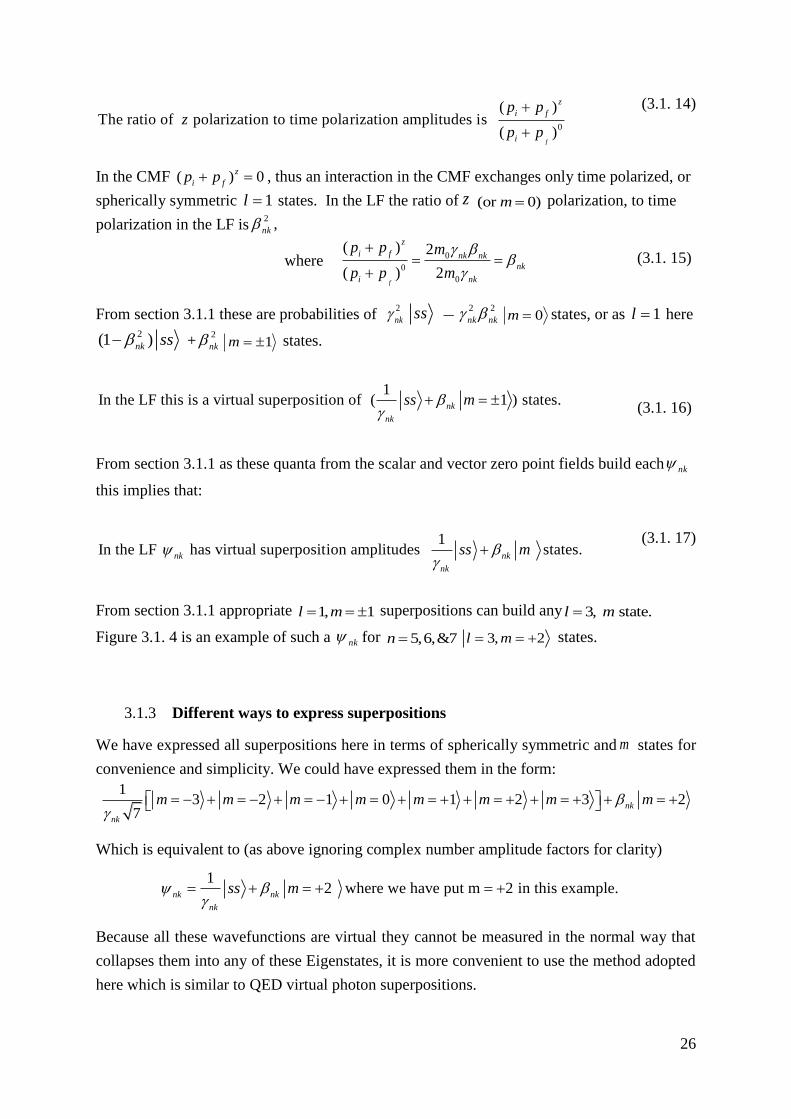
From section 3.1.1 appropriate 1, 1l m superpositions can build any 3, state.l m

Figure 3.1. 4 is an example of such a nk for 5,6,&7n 3, 2l m states.

3.1.3 Different ways to express superpositions

We have expressed all superpositions here in terms of spherically symmetric and m states for

convenience and simplicity. We could have expressed them in the form:

13 2 1 0 1 2 3 2

7nk

nk

m m m m m m m m

Which is equivalent to (as above ignoring complex number amplitude factors for clarity)

12 where we have put m 2 in this example.

nk nk

nk

ss m

Because all these wavefunctions are virtual they cannot be measured in the normal way that

collapses them into any of these Eigenstates, it is more convenient to use the method adopted

here which is similar to QED virtual photon superpositions.

27

Figure 3.1. 4 Eight preons forming 2m states as part of a positron superposition.

There is no significance in which preons absorb quanta in the above.

Any colour &

0p

28

3.2 Mass and Total Angular Momentum of Infinite Superpositions

3.2.1 Total mass of massive infinite superpositions

We will consider first the total mass of an infinite superposition, and to help illustrate,

consider only one integral n Eigenfunction nk at a time; temporarily assuming that the

amplitude nc of each nk

has magnitude 1n

c . Each time nk is born it borrows virtual mass

from a scalar Higgs field and virtual energy from vector zero point fields. Each time nk is

born the virtual mass that it borrows is exactly cancelled by an equal debt in the Higgs scalar

field so this should sum to zero for all k. But what about the momenta borrowed from the

zero point fields, do these momenta also leave momentum debts in the vacuum? From section

2.3.2 as k , 2 2 2

nk nkE c p 2 2 2

n or nkE n and n quanta of energy and

momentum k are absorbed. We know that in some unknown direction ,nk

np k which

implies these n absorbed quanta must leave a cancelling debt in the opposite direction of

( )nk

debt n p k in the vacuum. But this is true only as k &2

1nk

and the virtual

quanta energy transferred XE . So what happens when

21?

nk Our wavefunctions

nk are generated from a vector potential squared term 2

A derived in section 2.1.2 which in

turn came from a 2B type term as in section 2.1.1. As discussed in section 2.3.2 the

Eigenvalues

2 2 2 2

nkn kp confirm the constant momentum squared feature of magnetic type

interactions. Also in section 2.1.1 the scalar virtual photon emission probability is directly

related to the force squared term 2 2 2.F E Magnetic type coupling probabilities are related

to a magnetic type force squared term 2 2 2 2 2 2 2 2

/F B c E , where from section 3.1.2

and Eq’s. (3.1. 14) & (3.1. 15) the ratio of this scalar to magnetic coupling is2

.nk

Thus when

k and the exchanged energy XE ,

2

nkn quanta k are absorbed from the vacuum

and:

2

  We can expect a momentum debt of ) (nk nk

debt n p k (3.2. 1)

We could sum 2

nkp & 2( )

nkdebtp but both vectors nk

p and ( )nk

debtp are antiparallel in the

same unknown direction. We can pair them together giving a nett momentum per pair of:

2

2 2( ) ( ) ( at wavenumb . r ) e1 nk

nk nk nk nk

nk nk

nnett debt n k

pkp p p k

(3.2. 2)

We have said above that the mass of each virtual particle is cancelled by an equal and

opposite debt in the Higgs scalar field so we can now use the relativistic energy expression

2 2 2

0

( )k

n nk

k

E nett c

p times the probability of each pair at each wavenumber k.

We will initially look at only 1N massive infinite superpositions in Eq. (2.2. 4).

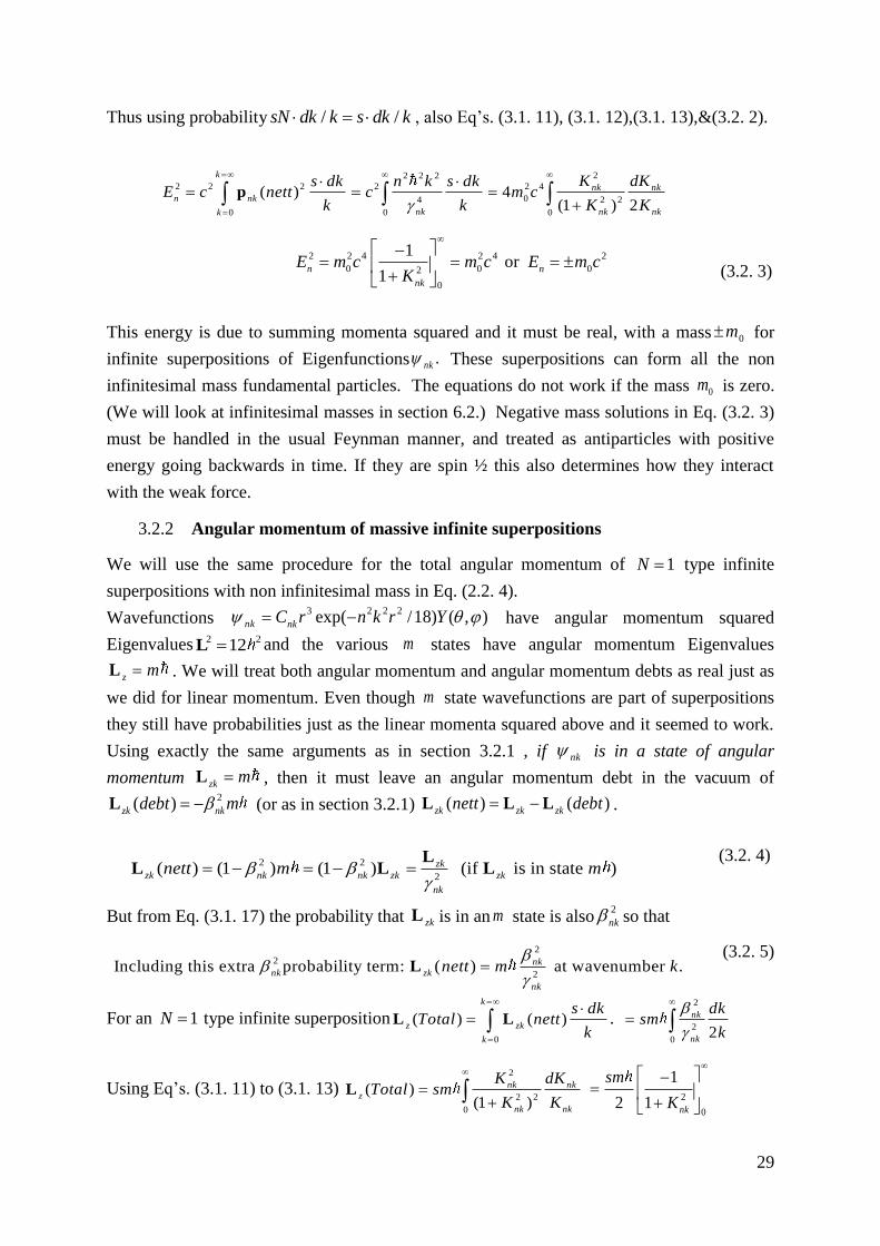
29

Thus using probability / /sN dk k s dk k , also Eq’s. (3.1. 11), (3.1. 12),(3.1. 13),&(3.2. 2).

2 2 2

0

( )

k

n nk

k

s dkE c nett

k

p

2 2 2

2

4

0 nk

n k s dkc

k

2

2 4

0 2 2

0

4(1 ) 2

nk nk

nk nk

K dKm c

K K

2 2 4 2 4 2

0 0 02

0

1 or

1n n

nk

E m c m c E m cK

(3.2. 3)

This energy is due to summing momenta squared and it must be real, with a mass 0m for

infinite superpositions of Eigenfunctions .nk

These superpositions can form all the non

infinitesimal mass fundamental particles. The equations do not work if the mass 0m is zero.

(We will look at infinitesimal masses in section 6.2.) Negative mass solutions in Eq. (3.2. 3)

must be handled in the usual Feynman manner, and treated as antiparticles with positive

energy going backwards in time. If they are spin ½ this also determines how they interact

with the weak force.

3.2.2 Angular momentum of massive infinite superpositions

We will use the same procedure for the total angular momentum of 1N type infinite

superpositions with non infinitesimal mass in Eq. (2.2. 4).

Wavefunctions nk 3 2 2 2

exp( /18) ( , )nk

C r n k r Y have angular momentum squared

Eigenvalues 2 212L and the various m states have angular momentum Eigenvalues

zmL . We will treat both angular momentum and angular momentum debts as real just as

we did for linear momentum. Even though m state wavefunctions are part of superpositions

they still have probabilities just as the linear momenta squared above and it seemed to work.

Using exactly the same arguments as in section 3.2.1 , if nk is in a state of angular

momentum zkmL , then it must leave an angular momentum debt in the vacuum of

2

( )zk nk

debt m L (or as in section 3.2.1) ( ) ( )zk zk zk

nett debt L L L .

2 2

2( ) (1 ) (1 ) (if is in state )zk

zk nk nk zk zk

nk

nett m m

L

L L L (3.2. 4)

But from Eq. (3.1. 17) the probability that zkL is in an m state is also

2

nk so that

2

2

2Including this extra probability term: ( ) at wavenumber .nk

nk zk

nk

nett m k

L (3.2. 5)

For an 1N type infinite superposition0

( ) ( )

k

z zk

k

s dkTotal nett

k

L L .

2

2

02

nk

nk

dksm

k

Using Eq’s. (3.1. 11) to (3.1. 13) 2

2 2

0

( )(1 )

nk nk

z

nk nk

K dKTotal sm

K K

L

2

0

1

2 1nk

sm

K

30

( ) or 2 2

z

sm sTotal m m m L

(3.2. 6)

Where m is the angular momentum state of the infinite superposition and m the state of nk .

Thus for spin ½ particles with s ½ in Eq.(3.2. 6) / 4m m but mcan be only ½,

implying the m state of nk that generates spin ½ must be 2m . An 1N massive spin 1

particle has 1s with / 2m m . ( 2N is covered in section 6.2.) This is summarized in

the following three member infinite superpositions ignoring complex number factors.

1/2, 1/2 2

5,6,

,1

2 , ,

07

1Massive ( 1) Spin ,

2

knk ss

n nk nk

nkkn

N c dkk

(3.2. 7)

1, 2

4,5,6

,

, ,

0

1Massive ( 1) Spin 1,

knk

m

ss

n nk nk

n

m

n kk

N c dkk

(3.2. 8)

The spin vectors of each nk with 2 3L , and their spin vector debts in the zero point

vector fields, have to be aligned such that the sum in each case is the correct value:

3 / 2L , 2L or 6L for spins ½ , 1 & 2 respectively. Gravity (the term) is

included in Eq. (1.1. 1) in our summary also spin 1 in Eq. (3.2. 8) is for 1N .

Spherically symmetric massive 1N spin 1 states are a superposition of three states

11 0 1 ,

3m m m and using Eq. (3.2. 8) can be formed as follows

,

,1, ,

4,5,6 0

1

,

,1, ,

4,5,6 0

,

,1, ,

4,5,6

2

0 0

1 2

1 1 1

3 3

1 1 1Massive spin 1

3 3

1 1

3 3

knk ss

n nk nk

n nkk

knk ss

n nk nk

n nkk

nk ss

n nk nk

n nk

m m

m m

m m

c dkk

c dkk

c

0

1k

k

dkk

(3.2. 9)

3.2.3 Mass and angular momentum of multiple integer n superpositions

In sections 3.2.1 & 3.2.2 for simplicity we looked at single integer n superpositions nk . For

superpositions k n nk

n

c , we replace 2

nkK with

2

kK . Equation (2.3. 9) appears to suggest

2 2 2 2 2 2 2*

k n n

n

c c n k n k p and 2

kk np . In section (3.5.1) we discuss why

2

kk np but *

k n n

n

k c c n k n p . Thus using Eq. (3.1. 11)

2 2 2 22 2 2 22

& but 2 2 2

C C C

k k k

k s k s k sK n K n K n

(3.2. 10)

31

Replacing2

nkK with

2 22 2/ 2

k CK k s n in the key equations (3.2. 3) & (3.2. 6) does not

change the final results. The laws of quantum mechanics tell us the total angular momentum

is precisely integral or half integral / 2 . Looking at the above integrals used to derive

total angular momentum we see that N must be 1 (we discuss N=2 in section 6.2) also s must

be exactly ½ or 1 for spin ½ & spin 1 massive particles respectively, in Eq. (2.2. 4) our

probability formula. Also these integrals are infinite sums of positive and negative integral

that are virtual and cannot be observed. If an infinite superposition for an electron is in a spin

up state and flips to spin down in a magnetic field, a real 1m photon is emitted carrying

away the change in angular momentum. This is the only real effect observed from this

infinity of ( 3, 2)l m virtual wavefunctions all flipping to ( 3, 2)l m states, plus an

infinite flipping of the virtual zero point vector debts. Also Eq’s. (3.2. 3) & (3.2. 6) are true

only if our high energy cutoff is at infinity and the low frequency cutoff is at zero. We look at

high energy Planck scale cutoffs in section 4.2 and in section 6.1 low energy cutoffs near the

radius of the causally connected horizon.

3.3 Ratios between Primary and Secondary Coupling

3.3.1 Initial simplifying assumptions

This section is based on a special case thought experiment that tries to illustrate, hopefully in

a simple way, how superpositions interact with one another; in the same way as virtual

photons interact with electrons for example. It is unfortunately long and not very rigorous,

but it illustrates how, in all interactions between fundamental particles represented as infinite

superpositions, the actual interaction is between only the same k single wavenumber

superpositions of each particle. We will later conjecture that the interacting virtual particle is

a single wavenumber k superposition only and not a full infinite superposition. Only real

particles whose properties we can measure are full infinite superpositions. The full properties

do not exist until measurement, just as in so many other examples in quantum mechanics.

This will be clearer as we proceed. It is also important to remember here that because

primary coupling constants are to bare charges (section 2.2.2), and thus fixed for all k, while

secondary coupling constants run with k, that the coupling ratios can be defined only at the

cutoff value of k applying to the bare charge (sections 4.1.1 & 4.2.2). From Table 2.2. 1 there

are 6 fundamental primary charges for electrons and positrons. But electrons and positrons

are defined as fundamental charges. In other words what we define as a fundamental electric

charge is in reality 6 primary charges. Of course we can never in reality measure 6 as their

effect is reduced by the ratio between primary and secondary coupling. Because

electromagnetic and colour coupling are both via spin one bosons their coupling ratios are

fundamentally the same but because of the above they are related simply as 26 36:1 .

1 36

= Colour EM

(3.3. 1)

We define the colour and electromagnetic ratios as follows (leaving gravity till section 6.2.5)

32

(Secondary) (Secondary)3

(Primary) 3 (Primary)

1 1 and

Colour EMS EMS

Colour Colour P EM EM EMP

(3.3. 2)

The secondary coupling constants 3 &

EMS S

are the bare charge values, both at the

fermion interaction cutoff near the Planck length Eq. (4.2. 11). Also we assumed in section

2.2.2 that 31;

P thus from Eq.(3.3. 2)

1 1 18

3 3@ 2.029 10

C S cutoffk GeV

(3.3. 3)

In other words provided 31,

P the ratio C

(or )Colour

is also the inverse of the colour

coupling constant 3 at the high energy interaction cutoff near the Planck length. In this

respect C or Colour

is the fundamental ratio we will use mainly from here on. From the

above paragraphs to find the coupling ratios we need secondary interactions that are between

bare charges. But this implies extremely close spacing where the effects of spin dominate. If

the spacing is sufficiently large the effects of spin can be ignored but then we are not looking

at bare charges. However we can ignore the effects of shielding due to virtual charged pairs

by imagining as a simple thought experiment, an interaction between bare charges even at

such large spacing. We can also simplify things further by considering only scalar or

coulomb type elastic interactions at this large spacing. We are also going to temporarily

ignore Eq. (3.3. 2) and imagine that we have only one primary electric and or one colour

charge. Consider two superpositions and (due to the above simplifying assumptions) imagine

them as spin zero charges. QED considers the interaction between them as a single covariant

combination of two separate and opposite direction non-covariant interactions (a) plus (b) as

in the Feynman diagram of Figure 3.3. 1 below. The Feynman transition amplitude is

invariant in all frames [9]. So let us consider a special simple case in a CM frame where we

have identical particles on a head on (elastic) collision path with spatial momenta:

a a b b p p p p (3.3. 4)

From Eq. (3.3. 4) the initial and final spatial momenta are reversed with mirror images of

each other at each vertex. Also in this simple special scalar case the transferred four

momentum squared is simply the transferred three momentum squared, where ignoring the

minus sign for 2

q in what we are doing here for simplicity:

2 2 2 2 2

( ) ( ) 4 4 .a a b b a b

q p p p p p p (3.3. 5)

33

Figure 3.3. 1 Feynman diagram of virtual photon exchange between two spin zero particles

of charge e .

Figure 3.3. 2 All Eigenfunctions nk in the groups of three overlap at a fixed wavenumber k.

If we look at Figure 3.3. 2 we see that at any fixed value of k, all modes nk in the groups of

three overlapping superpositions for the various spins ½, 1 & 2 occupy very similar regions

of space (provided they are all on the same centre.) The directions of their linear momenta are

unknown but let us imagine some particular vector k that is parallel to the above vectors

a bp p . As we are considering only scalar interactions, all these modes must be spherically

symmetric (as in section 3.2.2 for spins 1 & 2, and for spin ½ provided or in turn nk

k is small

enough the probability that it is not spherically symmetric can be extremely low) and at a

fixed value of k they have momenta n k . Also as they overlap each other we can imagine

units of k quanta somehow transferring between these superpositions so that the values of

n in each mode can change temporarily by 1 for times /T E . The directions of these

(a) (b)

The Feynman diagram is drawn with

a vertical photon line representing

the superposition of two opposite

direction and non covariant

processes (a) plus (b).

The exchanged 4 momentum is:

.

Spin ½ Fermion

superpositions

Infinitesimal mass

spins 1 & 2

Boson superpositions

3( 3)

kn

Massive spin 1

Boson superpositions

34

momentum transfers causing either repulsion or attraction depending on the charge signs of

the superpositions at each vertex, whether the same or opposite.

3.3.2 Restrictions on possible Eigenvalue changes

Before we look at changing these Eigenvalues by 1n we need to consider what

restrictions there are on these changes.

From Eq. (2.3. 12) superposition k requires

2 2Q A

4 2 4 2

*81

n n

n

n k rc c and Eq. (2.2. 4) tells

us the available

2

2 2 2 4 28 8

3

EMP

sQ A k r

N

occurs with probability k

sN dk .

For very brief periods the required value of 2 2

Q A can fluctuate, such as during these changes

of momentum, but if its average value changes over the entire process then Eq. (2.2. 4) tells

us that probability /sN dk k changes also, and we have shown in section 3.2.1 that this is not

allowed. For example in a spin ½ superposition 5 6 7, , ,

k k k the average values of

5c ,

6c &

7c must each remain constant. This can happen only if n remains within its pre-existing

boundaries of (5 7)n . For example if 7 adds k , it can create 8

, but8

c must average

zero, which it can do only if it fluctuates either side of zero, andn

c cannot be negative.

Similarly4

c must average zero, thus 4 & 8

are forbidden states. Keeping the average

values ofn

c constant is also equivalent to a constant internal average particle energy (we

have shown in section 3.2.1 that rest mass is a function of2

* .n n nk

c c p ). By changing these

Eigenvalues by 1n there are only four possibilities; 6 & 7

can both reduce by k

quanta, 6 & 5

can both increase by k quanta. If 6 becomes 7

, 7

c also increases and

6c decreases, but then 7

has to drop back becoming 6, with

7c decreasing back down and

6c increasing back up in exact balance. If we view this as one overall process the average

values of both6

c and7

c remain constant but fluctuate continuously. We can use exactly the

same argument if 5 increases which has to be followed by 6

dropping, where if we view

this as one process again, the average values of both 5c and 6

c remain constant. This is

similar to a particle not being able to absorb a photon in a covariant manner, it has to reemit

within time / .T E With spherical symmetry the momentum .n p k If we change n

by 1 the sign of n p k determines the direction of the momentum transfer .p In the

above if 5 6k k

then returns 6 5

,k k

and n p k keeps the same sign during this

process, there is no nett momentum transfer and there is a probability of this, but it is not the

probability we need. However consider the process as in Figure 3.3. 3.

To get a net momentum transfer the momenta have to be in opposite directions for each half

of this process. (Conservation of momentum allows this only if there is an equal and opposite

transfer of momentum at the other vertex of the interaction.) The problem with this is that a

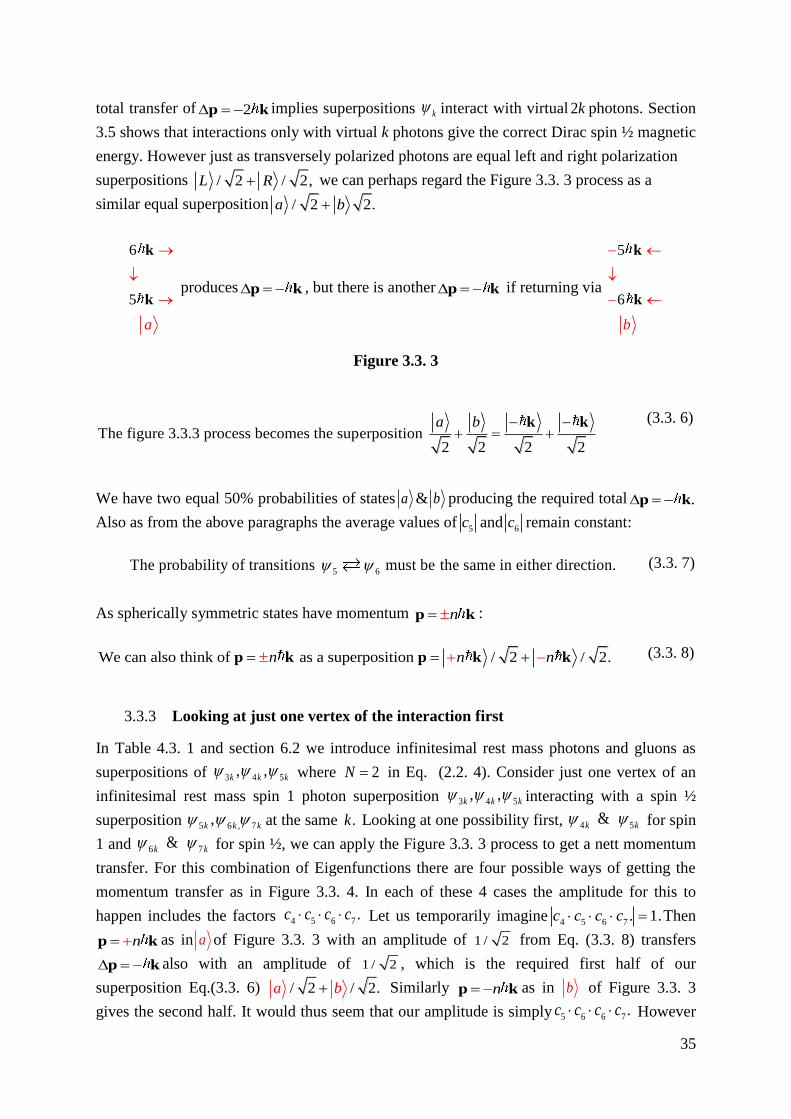
35

total transfer of 2 p k implies superpositions k interact with virtual 2k photons. Section

3.5 shows that interactions only with virtual k photons give the correct Dirac spin ½ magnetic

energy. However just as transversely polarized photons are equal left and right polarization

superpositions / 2 / 2,L R we can perhaps regard the Figure 3.3. 3 process as a

similar equal superposition / 2 2.a b

6

5

a

k

k produces p k , but there is another p k if returning via

5

6

b

k

k

Figure 3.3. 3

The figure 3.3.3 process becomes the superposition 2 2 2 2

a b

k k

(3.3. 6)

We have two equal 50% probabilities of states a & b producing the required total . p k

Also as from the above paragraphs the average values of5

c and6

c remain constant:

5 6The probability of transitions must be the same in either direction. (3.3. 7)

As spherically symmetric states have momentum n p k :

We can also think of as a superposition / 2 / 2.n n n p k p k k (3.3. 8)

3.3.3 Looking at just one vertex of the interaction first

In Table 4.3. 1 and section 6.2 we introduce infinitesimal rest mass photons and gluons as

superpositions of 3 4 5, ,

k k k where 2N in Eq. (2.2. 4). Consider just one vertex of an

infinitesimal rest mass spin 1 photon superposition 3 4 5, ,

k k k interacting with a spin ½

superposition 5 6 , 7,

k k k at the same .k Looking at one possibility first, 4 5

& k k

for spin

1 and 6 7 &

k k for spin ½, we can apply the Figure 3.3. 3 process to get a nett momentum

transfer. For this combination of Eigenfunctions there are four possible ways of getting the

momentum transfer as in Figure 3.3. 4. In each of these 4 cases the amplitude for this to

happen includes the factors 4 5 6 7.c c c c Let us temporarily imagine

4 5 6 7. 1.c c c c Then

n p k as in a of Figure 3.3. 3 with an amplitude of 1 / 2 from Eq. (3.3. 8) transfers

p k also with an amplitude of 1 / 2 , which is the required first half of our

superposition Eq.(3.3. 6)

/ 2 / 2.a b Similarly n p k as in b of Figure 3.3. 3

gives the second half. It would thus seem that our amplitude is simply 5 6 6 7.c c c c However

36

from Eq. (3.3. 7) there is a 50% probability of the transitions 5 6 in either direction, or

an extra 1 / 2 amplitude factor for 5 6 in either direction, similarly an extra 1 / 2

amplitude factor for 6 7. These two extra 1 / 2 factors reduce the amplitude

4 5 6 7 toc c c c

4 5 6 7 / ( 2 2)c c c c 4 5 6 7

/ 2.c c c c Thus adding the four cases in

Figure 3.3. 4 together and treating all other factors as 1:

Figure 3.3. 4 process amplitude factor is 4 5 6 7 4 5 6 7 4 ( ) / 2 2c c c c c c c c (3.3. 9)

Figure 3.3. 4

The four possibilities in Figure 3.3. 4 are all between the same sets of Eigenfunctions

4 5&

k k for spin 1, 6 7

&k k

for spin ½. But there are also four different sets of these A, B,

C & D, between groups of four Eigenfunctions as in Figure 3.3. 5; with their amplitudes from

Eq. (3.3. 9) below each relevant box, which we also label as A, B, C & D. (Subscripts a refer

to spin ½ and b to spin 1.)

A B C D

Amplitudes: 4 5 6 72 ,

b b a aA c c c c 3 4 6 5

2 ,b b a a

B c c c c 4 5 6 5

2 ,b b a a

C c c c c 3 4 6 7

2 .b b a a

D c c c c

Figure 3.3. 5

Spin 1

4 goes to 5

with

5 returns to 4

with

Spin 1/2

7 goes to 6

with

6 returns to 7

with

Spin 1

4 goes to 5

with

5 returns to 4

with

Spin 1/2

6 goes to 7

with

7 returns to 6

with

Spin 1

5 goes to 4

with

4 returns to 5

with

Spin 1

5 goes to 4

with

4 returns to 5

with

Spin 1/2

7 goes to 6

with

6 returns to 7

with

Spin 1/2

6 goes to 7

with

7 returns to 6

with

Spin 1 Spin ½

5 7

4 6

3 5

Spin 1 Spin ½

5 7

4 6

3 5

Spin 1 Spin ½

5 7

4 6

3 5

Spin 1 Spin ½

5 7

4 6

3 5

37

3.3.4 Assumptions when looking at both vertexes of the interaction

Because we are looking at an interaction between identical spin ½ fermions each vertex has

the same groups of Eigenfunctions A,B,C&D as in Figure 3.3. 5. From section 2.2.2 and

Figure 3.1. 4 the three Eigenfunctions forming each of the interacting particles are born

simultaneously. It would thus seem reasonable to assume that the amplitudes of each group of

three Eigenfunctions have the same complex phase angle. The two fermions and one boson

can be at different complex phase angles to each other but each one individually is a

superposition of three Eigenfunctions at the same complex phase angle. Thus the four

amplitudes A,B,C&D from Figure 3.3. 5 (A,B,C &D each comprising two fermion amplitudes

and two boson amplitudes) must all have the same complex phase angle. Similarly the four

amplitudes , , &A B C D of vertex 2 in Figure 3.3. 6 also have a common phase angle.

Eigenfunction

Groups

A B C D

Vertex 1 Amplitude A Amplitude B Amplitude C Amplitude D

Vertex 2 Amplitude A Amplitude B Amplitude C Amplitude D

Figure 3.3. 6

We are also going to assume that Eigenfunctions A of vertex 1 interact only with

Eigenfunctions A of vertex 2 and Eigenfunctions B of vertex 1 interact only with

Eigenfunctions B of vertex 2 etc. Eigenfunctions A of vertex 1 do not interact with

Eigenfunctions B of vertex 2 etc. Thus if all other amplitude factors are 1:

The total interaction amplitude AA BB CC DD (3.3. 10)

Apart from a different complex phase angle this is equivalent to: ( & , &A A B B etc. all

differ by the same complex phase angle.)

2 2 2 2

Total interaction amplitude A B C D (3.3. 11)

2 2 2 2 2 2 2 2

Interaction probability ( )* ( )A B C D A B C D

(3.3. 12)

Using 2 2

( * ) ( * )( * ) etc. this is equivalent toA A A A A A

2

Interaction probability ( * * * * )A A B B C C D D (3.3. 13)

38

From Figure 3.3. 5 4 5 6 72 ,

b b a aA c c c c 3 4 6 5

2 ,b b a a

B c c c c4 5 6 5

2 ,b b a a

C c c c c3 4 6 7

2 .b b a a

D c c c c

5 5 5 4

22

4 5 6 7 3 4

4 4 4

6

5 6 7

5 4 5 6 5 3 4 6 7

Putting etc. & etc. this is equivalent to

( * * * * ) 16

* , *

* 4

b b a a b b a a b b a a

a a

b

a b b b b b a

b a

a

aA A B B C C D D P P P P P P P P P P P

P c c P c c A A P P P P

P P P P P

2 2

4 3 5 6 5 7 = 16 ( ) ( )

b b b a a aP P P P P P

Then using 3 3 4 4 5 5 5 5 6 6 6 6* * * * * * 1

b b b b b b a a a a a ac c c c c c c c c c c c the interaction probability is

2

4 4 4 4

4

6

2 2

6 6 6* (1 * (1*( * * * * ) 2 )) *

b b b b a a a aA A B B C C c c c c cc c cD D

(3.3. 14)

We have assumed to here that all other amplitude factors are 1. However at each vertex there

are both fermion and boson superposition probabilities from Eq. (2.2. 4). Writing the

superposition probability at each vertex /sN dk k as 1/2 1/ ,s N dk k 1 2

/s N dk k for clarity

where 1 1 spin 1 , 1 is etc.s N N Including these factors (if all other factors are one) in Eq.

(3.3. 14) our overall probability at wavenumber k is

2

1/2 1 6

2

1 2 4 4 46 6 462 * (1 * 2 (1) * * )

b b ba ba a as N c c c c s N c c c c

kk

22

1/2 1 6 1 2 4 4 4 46 6

4

62 *2 * (

.(

(1 )1 * ) *

)

a a a b ba b bss N c c c c N c c c c

k

The momentum per transfer is a total of k and using Eq’s. (3.3. 5), (3.3. 6) & Figure 3.3.

3 we have 4 4

( ) q k (then putting 1 ) the interaction probability:

2

1/2 1 6

2

1 2 4 4 46 6 4

4

62 *2 * ( )1 () 1* *

a a b b ba a bs N c cs N c

q

c c cc c

(3.3. 15)

This is the scalar interaction probability between two spin ½ fermions exchanging

infinitesimal rest mass spin 1 bosons at very large spacings, where the fermions are

effectively spin zero, imagining them as bare charges and all other factors being one. Going

through exactly the same procedure but similarly exchanging spin 2 infinitesimal rest mass

39

scalar gravitons (with 22N N for clarity) the gravitational interaction probability

between fermions becomes (using subscript c for spin 2) if all other amplitude factors are 1:

2

2 2 4 4

2

1/2 1 6 6 6 4 46

4

2 * for fermion

2 *s.

1 * *( (1) )a a c c c ca a

s N c c s N c c cc c c

q

(3.3. 16)

And if for example two spin 1 photons exchange spin 2 gravitons (all infinitesimal rest mass

with 22N N ) the interaction probability becomes if all other amplitude factors are 1:

2

1 2 4

2

2 24 4 4 44 4

4

42 *

for 2 pho(12 *

tons.( )* 1 * )

b b b b c c c cs N c cs N c c c c c c

qN

(3.3. 17)

If two massive 1N photons (as in Figure 3.3. 2) exchange spin 2 gravitons the interaction

probability becomes if all other factors are 1:

2

1 1 5

2

2 25 4 4 45 4

4

52 *

for 1 pho(12 *

tons.( )* 1 * )

b b b b c c c cs N c cs N c c c c c c

qN

(3.3. 18)

General Relativity (section 1.1.1) tells us the emission of gravitons is identical for both mass

and energy. Keeping all other factors (such as mass/energy) in Eq’s. (3.3. 16), (3.3. 17) &

(3.3. 18) constant, the exchange probabilities must be the same in each. We can thus put them

equal to each other and cancel out the red terms:

1 2 4 4 4 4 1 1 5 5 1/2 1 65 5

5 5 5 5

6 6

4

6

4 4 4

or

   

2 * (1 * )

2 * (1

2 * (1 * )

4 *

2 * (1 * )

(1 * ) * )

b b b b

b b b b

a a a ab b b b

b b b b

s N c c c c

c c c c

s N c c cs N c c c c

c c c

c

c

6 6 6 6

1 S pin 1

* (1 * )

1 Sp in 2 Spin 1 1/2

a a a ac c

NN

c c

N

(3.3. 19)

Now assume that all other factors (other than coupling constants) are 1, and remember that

we are simplifying with a thought experiment by looking at spin ½ superpositions sufficiently

far apart so we can treat them as approximately spherically symmetric or effectively spin zero

even if they are supposed to be bare charges with spin. Under these same scalar exchange

conditions QED tells us that with electrons for example:

The probability of scalar or coulomb exchange in Eq (3.3. 15). 2

4

4= . 

q

(3.3. 20)

40

Let us temporarily ignore the fact that gluons have limited range, and imagine our thought

experiment applying to colour charges exchanging gluons. The of Eq. (3.3. 20) becomes

the usual colour coupling 3 . To get the fundamental coupling ratio labelled as C

1

3

@cutoff

k we substitute the of Eq. (3.3. 20) with1

C

as we have assumed

3(Primary) 1.

Also substitute 1/2 12 1, 2 2,s s

1 21 & 2N N and equate Eq’s. (3.3. 15) & (3.3. 20)

1 2

4

2

6 6 6 6

2

4 4 4 4

4 4 46 6 6 46

4

1

4 * (1 * )

4 * (1 *or 2

* ( 4( )1 * )

* ( * ) )1

b b b b

b b b b

a a a a

a

C

Ca a a

q

c c c c

c c c c

c c c c

c c c c

q

(3.3. 21)

But from Eq. (3.3. 19) the blue and green terms are equal (also the magenta terms) and we

can solve for the fundamental coupling ratio by combining Eq’s. (3.3. 19) & (3.3. 21).

4 4 6 6 6 65 5 54 4 5

1 Spin 1

Massive Phot

1 Spin 1/2

2 Spin 1

Ph Fermiootons or Gluons

ons

2 * (1 * )

ns

* (14 * (1 * ) * )b a ab ab b bb bb a

N

c c c

N N

cc c c cc cc c

1

2

C

(3.3. 22)

The coupling ratio is fundamentally the same for colour and electromagnetism apart from the

six primary electric charges of Eq. (3.3. 1) because of the way electric charge is defined.

Equations (3.3. 19), (3.3. 21) & (3.3. 22) tell us that for any interactions between two

superpositions, the inverse coupling ratio always involves the product of the central

superposition member probability by the probability of the other two members combined

N spin of the first superposition, times the equivalent product for the other superposition.

In section 4 we introduce gravity and solve these ratios. Despite all the simplifications and

lack of rigorousness, the above equations are surprisingly consistent with the Standard

Model, provided there are only three families of fermions. Even though we used gravity to

derive Eq.(3.3. 19) we leave discussing the gravity coupling ratio till section 6.2.5.

3.4 Electrostatic Energy between two Infinite Superpositions

3.4.1 Using a simple quantum mechanics early QED approach

In section 3.3 we have shown that fermion superpositions can exchange boson superpositions

in the same way as electrons can exchange virtual photons for example. Providing the

superposition amplitudes are appropriate, the coupling constants can be just as in QED,

though we will look further at this in section 4.1.1. So it might seem that evaluating

electrostatic energy between superpositions is unnecessary. However when we look at gravity

41

we find that the spacetime warping around mass concentrations appears to be strongly related

to cosmic wavelength virtual graviton probability densities. Virtual particle exchange

probabilities, in QED/QCD etc, use perturbation theory to calculate particle scattering

crossections, and electron g factor corrections with incredible precision; but as we later focus

on virtual graviton probability densities, it is more appropriate here to use a simple, but only

approximate, quantum mechanical method based on virtual photon probability densities to

find the scalar potentials between two charges (or infinite superpositions). This same method

also allows a simple solution to the magnetic energy between superpositions in Section 3.5,

where we modify relevant equations in a simple manner. We later use some of these same

equations when looking at why borrowing energy and mass from zero point fields, requires

the universe to expand after the Big Bang, and distort spacetime around mass concentrations.

We assume spherically symmetric 3l superpositions emit virtual scalar photons in this

section and 3, 2l m superpositions emit virtual 1m photons in section 3.5. As

section 3.3 has shown that we can achieve the same electromagnetic coupling constant we

can use the scalar photon emission probability (2 / )( / )dk k covered in section 2.1.1. From

section 3.3 we can also see that the effective average emission point has to be the center of

superpositions. For a virtual photon / 2E T , and the range over which it can be found

is roughly r T 1/ 2 1/ 2E k when 1c . The radial probability of finding the

centre of the spin 1 superposition representing the interacting virtual photon decays

exponentially with radius as 2kre . The normalized wavefunction for such a virtual scalar

photon of wave number k emitted at 0r is:

( )

2 2 @ time 0.

4 4

kr i kr t kr ikrk e e k e e

tr r

kr

Figure 3.4. 1 Radial probabilities of 6k and the exponential decay with radius of a virtual

photon of the same k value 2* 2 .

krR R ke

These curves look the same for all k , applying

equally to virtual photons, gravitons and to large k value gluons etc.

Radial probability of finding the virtual photon

superposition centre of the same k value.

4 *R R

k

Dominant fermion virtual wavefunction 6k

42

Wavefunction is spherically symmetric as scalar photons are time polarized. Figure 3.4. 1

plots the radial probabilities of the exponentially decaying with radius virtual photon and the

dominant 6n mode of its relating superposition .k

The effective range of a wavenumber

k virtual photon is of a similar order to the radial probability dimensions of 6.

k For

simplicity in what follows we locate two superpositions (which we refer to as sources) in

cavities that are small in relation to the distance between them. The accuracy of our results

depends on how far apart they are in relation to the cavity size. Consider two spherically

symmetric sources distance 2C apart emitting virtual scalar photons as in Figure 3.4. 2

where point P is 1r from source 1, & 2r from source 2. Let 1 be the amplitude from source

1, and 2 be the amplitude from source 2 and for simplicity and clarity let 0t .

1 1 2 2

1 2

1 2

2 2Thus &

4 4

kr ikr kr ikrk e k e

r r

(3.4. 1)

Consider 1( 2 ) * 1( 2 ) 1 1 1 2 2 1 2 2* * * *

Now 1 1* & 2 2* are just the normal probability densities around sources 1 & 2 as

though they are infinitely far apart but the work done per pair of superpositions k on

bringing 2 sources closer together is in the interaction term: 1 2 2 1* * .

1 2 1 2

1 2

1 2

2*

4

kr kr ikr ikrke e e e

r r

1 2 1 2

( ) ( )

1 2

2

4

k r r ik r rke e

r r

2 1 2 1

2 1

1 2

2*

4

kr kr ikr ikrke e e e

r r

1 2 1 2

( ) ( )

1 2

2

4

k r r ik r rke e

r r

1 2 2 1* * 1 2 1 2 1 2( ) ( ) ( )

1 2

2

4

k r r ik r r ik r rke e e

r r

1 2( )

1 2

1 2

4cos ( )

4

k r rke k r r

r r

1 2 1 2 1 2 2 1

1 2

4Now put ( , ) & * * cos( )

4

AkkA r r B r r e kB

r r

(3.4. 2)

Real work is done when bringing superpositions together and we can treat these interacting

virtual photons as having real energy kc . Using virtual photon emission probability

(2 / )( / )dk k from section 2.1.1

2Energy per virtual photon Probabil   Probability

2ity

dkkc

cd

kk

(3.4. 3)

43

Figure 3.4. 2

Including Eq.(3.4. 3) the interaction energy @ k is thus ( 1 2 2 1* * )2 c

dk

and

using Eq. (3.4. 2) the interaction energy @ k is 2 c

dk

1 2

4cos( )

4

Akke kB

r r

.

The total interaction energy density due to 1 2 2 1* * for all k is

1 2 0

2 4cos( )

4

Akcke Bk dk

r r

(3.4. 4)

2 2

2 2 2

0

cos( )( )

Ak A Bke Bk dk

A B

(3.4. 5)

Where 2 2 2 2

1 2 1 1 2 2( ) 2A r r r r r r & 2 2 2 2

1 2 1 1 2 2( ) 2B r r r r r r

2 2 2 2 2 2 2 2

1 2 1 1 2 2 1 2Thus ( ) 2 & 2( )A r r r r r r A B r r (3.4. 6)

2 2

2( )r C as cos(180 ) cos

2 2 2 2

and 4( )A B r C (3.4. 7)

Putting Eq’s. (3.4. 4), (3.4. 5), (3.4. 6) & (3.4. 7) together 2 2

1 2

2 2 2 2 2 2

4

( ) 16( )

r rA B

A B r C

0

cos( )Ak

ke Bk dk

1 2

2 2 24( )

r r

r C

Source 1 Source 2

Point P

44

1 2 0

2 4cos( )

4

Akcke Bk dk

r r

1 2

2 4

4

c

r r

1 2

2 2 24( )

r r

r C

1 2 0

2 4cos( )

4

Akcke Bk dk

r r

2 2 2

2 1 1

4 ( )

c

r C

(3.4. 8)

This is the total interaction energy density of time polarized virtual photons at point P due to

1 2 2 1* * for all k and there are no directional vectors to take into account. We will

use similar equations for the vector potential ( 1m ) photons for magnetic energies but will

then need directional vectors. Equation (3.4. 8) is the energy due to the interaction of

amplitudes at any radius r from the centre of the pair. It is independent of , and to get the

total energy of interaction we multiply by 2

4 r dr for layer dr and integrate from 0 .r

The total interaction energy is 1 2 2 1

0 0

2( * * )

cdk

2

4 r dr

Using Eq. (3.4. 8) 2 1

4

c

2

2 2 2

0

4

( )

r dr

r C

Thus 1 2 2 1

0 0

2( * * )

cdkdv

2 c

2

2 2 2

0( )

r dr

r C

2

2 2 2

0( )

r dr

r C

1

2 2C

The interaction or potential energy is  2

  c c

C R

(3.4. 9)

If 2R C is the distance between the centres of our assemblies, this is the classical potential.

The procedure used here with small changes, simplifies the derivation of the magnetic

moment; we reuse some equations, but in a slightly modified form taking polarization vectors

into account. We also reuse some of these simple but approximate derivations when looking

at gravity in Section 5.

45

3.5 Magnetic Energy between two spin aligned Infinite Superpositions

In this section we are going to consider two infinite superpositions that form Dirac spin ½

states. We will look at the magnetic energy between them when they are both in a spin up

state say along some z axis as in Figure 3.5. 1. We are not looking at the magnetic energy

here when they are both coupled in a spin 0 or spin 1 state. That is, both Dirac spin ½ states

have their 3 / 2 spin vectors randomly oriented around the z axis with / 2 components

aligned along this z axis. Also in this section we will be dealing with transversely polarized

virtual photons and must take account of polarization vectors. In section 3.2.2 and Eq. (3.2. 7)

spin ½ states are generated only from 3, 2l m states and as transversely polarized photons

are superpositions of 1m photons they can only be emitted from these 3, 2l m states,

the remaining states are spherically symmetric and cannot emit transversely polarized

photons. We don’t yet know the value of amplitudes nc so we will derive the magnetic

energy in terms of these. We will then equate this energy to the Dirac values assuming a g

value of 2 before QED corrections; this allows us to evaluate in section 4.3 the amplitudes

nc in terms of the ratio EM between primary and secondary electromagnetic coupling. We

can then evaluate in section 4.1 the primary electromagnetic coupling constant EMP in terms

of the ratio EM . (Section 3.5 uses the same format as Chapter 18, “The Feynman Lectures on

Physics” Volume 3, Quantum Mechanics [11].)

Figure 3.5. 1

An 3, 2l m state can emit a right hand circularly (R.H.C.) polarized ( 1)m photon in

the z direction. Let the amplitude for this be temporarily R .

An 3, 2l m state can emit a left hand circularly (L.H.C.) polarized ( 1)m photon in

the z direction. Let the amplitude for this also be temporarily L .

First rotate the z axis about the y axis by angle (call this operation S R ) then use

(1/ 2)x R L and multiply on the right by operation S R .

46

The amplitude to emit a transversely polarized photon in the x direction is thus

1

2x S R R S R L S R

Where 2 23, 2 3, 2 (1 / 4) 2 2 cos 4sin 3sin cosR S R S

is the

amplitude an 3, 2l m state remains in an 3, 2l m state after rotation by angle .

Also 2 23, 2 3, 2 (1 / 4) 2 2 cos 4sin 3sin cosL S R S

is minus the

amplitude that an 3, 2l m state is in an 3, 2l m state after rotation by .

Putting this together 2

1 2 sin cos 2

2 2x S R

(3.5. 1)

An 3, 2l m state can also emit an ( 1)m photon in the z direction but it will now be

left hand circularly polarized. Let this amplitude be temporarily: L .

Similarly an 3, 2l m state can emit an ( 1)m photon in the z direction which is right

hand circularly polarized. Let this amplitude be temporarily: R .

We can go through the same procedure as above to getcos 2

2x S L

(3.5. 2)

This amplitude Eq. (3.5. 2) is for a photon emitted in the opposite direction to amplitude Eq.

(3.5. 1) but cos2 cos2(180 ) and we can simply add these two amplitudes. Let us

assume however that an 3, 2l m state has equal amplitudes to emit in the z & z

directions of / 2R and / 2L .

With these amplitudes; 1 cos 2 cos 2

2 22x S R x S L

cos 2

(3.5. 3)

Eqation (3.5. 3) is the angular component of the amplitude for a transverse x polarization in

the new z direction where x x & z z . When 0 or 180 the on axis amplitude

for transverse polarization is one as expected ignoring other factors. Using the same

normalization factors (we check the validity of this in section 3.5.2 we can still use the

amplitudes and phasing of our original time mode photons Eq’s. (3.4. 1) but instead of

including polarization vectors we will for simplicity just use the cosine of the angle ( )

between them (as in Figure 3.5. 2 ) as a multiplying factor. Including the angular factor Eq.

(3.5. 3) in our earlier scalar amplitudes Eq’s. (3.4. 1) we have for our new wavefunctions:

47

1 1 2 2

1 2

1 2

2 2cos 2 & cos 2

4 4

kr ikr kr ikrk e k e

r r

(3.5. 4)

The transverse polarized photons from sources (1) & (2) have polarization vectors 1x and

2x at angle to each other ( ) , (Figure 3.5. 2) and the complex product becomes:

1( 2 ) * 1( 2 ) 1 1 1 2 2 1 2 2* ( * * )(cos( ) *

Where the interaction term is now: 1 2 2 1( * * ) cos( ) and as in the scalar case

(section 3.4.1) but now using Eq’s. (3.5. 4)

1 2 1 2( ) ( )

1 2

1 2

2* cos( ) cos 2 cos 2 cos( )

4

k r r ik r rke e

r r

1 2 1 2( ) ( )

2 1

1 2

2* cos( ) cos 2 cos 2 cos( )

4

k r r ik r rke e

r r

1 2 2 1

1 2

4( * * ) cos( ) cos 2 cos 2 cos( )

4

Akke kB

r r

cos( )

(3.5. 5)

(Where as in section 3.4.1, Eq. (3.4. 2) 1 2 1 2&A r r B r r . )

Figure 3.5. 2 Two sources 2C apart, both with 2

( 2)nk m states along the joining line,

& are the respective angles to P , 1r & 2r are the respective distances to point P.

3.5.1 Amplitudes of transversely polarized virtual emmited photons

In the laboratory frame nk has amplitude nk to be in an 2m state (section 3.1). For a

multiple integer n superposition k n nk

n

c . At each fixed wavenumber k we cannot

C C

Source 1 Source 2

Point

48

distinguish which integer n a virtual photon comes from, so we must add amplitudes from

each individual integer n superposition. To keep integrals simple we will assume that

1nk or that spacing 2C is very large, and our interacting k values are very small.

(We can make a comparison with the Dirac values at any large spacing so accuracy need not

be affected.) Thus if 1nk & 1nk , we can approximate Eq. (3.1. 11) as

0 0

2 22

2 2 2 2

nk c c

nk nk nk nk

s nk s nkn k sK

m c m c

p for spin ½ fermions.

Adding amplitudes for multiple integer superpositions2

c

k

n kn

(3.5. 6)

(When deriving Eq. (3.2. 10) we said2

k k

k n and not k n p p . How do we

justify this? When 1nk as above nk n k nk

p So adding ampitudes nk to getk

is equivalent to adding nkp to get

kp and not adding

2 2 2 2

nkn kp to get

2.

kk np If

this is true when 1nk it must be true for 0 1.)nk

3.5.2 Checking our normalization factors

Let us pause and check the reasonableness of all this and our normalization factors. From

Eq’s. (3.4. 1) for scalar photons 2

2

2*

4

krk e

r

(emission probability2 dk

k

) gives a

Scalar k emission probability density

2

2

2 22*

4

krk e

r

dk dk

k k

.

The transversely polarized probability density, using Eq’s. (3.5. 4) & (3.5. 7) plus2

k is

Transverse emission probability density 2

2

2

2 2 2* cos 2

4

2 2nk

r

nk

kk e

r

dk dk

k k

(Where 1 22 2 & .r r ) If we now consider the on axis 0 case the transverse polarized

on axis emission probability density at k is:

2

2

2 22

4

kr

k

k dk

k

e

r

2

k 2

*dk

k

Just as in QED the factor2

k is the factor we need for this on axis emission probability

density ratio between transverse and scalar polarization. This justifies using the same

49

normalization constant 2 / 4k for both the scalar and magnetic wavefunctions. We seem to

be on the right track and using the same virtual photon emission probability and energy kc

as in Eq. (3.4. 3) for both the scalar and transverse polarization cases ie

2

Energy per transverse photon Probability   Probability 2dk

kcc

kk

d

(3.5. 7)

Multiplying Eq. (3.5. 5) by Eq. (3.5. 6) squared, and Eq. (3.5. 7) we get the transverse

interaction energy @ wavenumber k :

2

1 2 2 1( * * ) cos( )k 2 c

dk

22 2

1 2

4cos 2 cos 2 cos( )

4 4

C Akn k ke kB

r r

cos( ) 2 c

dk

Rearranging this: 2

1 2 2 1( * * ) cos( )k 2 c

dk

=

2 22 Cn c

1 2

cos 2 cos 2 cos( )

4 r r

3cos( )

Akk e kB dk

(3.5. 8)

As in the scalar case we integrate over k first but now with a 3

k term due to the inclusion of

the2

k factor which is approximately proportional to2

k from Eq. (3.5. 6).

Using 1 2 1 2 & A r r B r r and Eq’s. (3.4. 6) & (3.5. 6)

3

0

cos( )Ak

k e kB dk

=

2 2 2 2 21 2

2 2 4

2 ( )3

8 ( )

r r r C

r C

And thus: 2

1 2 2 1

0

( * * ) cos( )k

2 c

dk

=

2 22 Cn c

1 2

cos 2 cos 2 cos( )

4 r r

2 2 2 2 21 2

2 2 4

2 ( )3

8 ( )

r r r C

r C

(3.5. 9)

Equation (3.5. 9) is the magnetic interaction energy density at point P for all wave numbers .k

Figure 3.5. 2 is a plane of symmetry that can be rotated through angle 2 around the axis of

symmetry (the joining line along the axis of the 2 spin aligned sources). To evaluate the total

magnetic energy density over all space we just multiply by 24 sin .r d dr

50

We thus integrate Eq. (3.5. 9) 24 sin .r d dr =

2 2 /2 2 2 2 2 2

21 2

2 2 4

1 20 0

3 2 ( )cos 2 cos 2 cos( )sin

4 ) 

(

Cn c r r r C

r d drr r r C

(3.5. 10)

Now 2

1 20 0

cos 2 cos 2 cos( )

r r

2 2 2 2 21 2

2 2 4

2 ( )

( )

r r r C

r C

2sinr d dr can be reduced to the

single integral:

1 22

3 3 2

0

1 (7 5 ) 1 14 161 ln

1 38

x xx dx

xC x x

which can be also expressed

as an infinite series in p (to not confuse with superposition value n ):

3

1

8C 1

14 10 (2 1)!.

2 3 2 1 2( 1)!( 1)!4

p

pp

p

p p p p

3

1 (160 51 ).

6 28C

3

1 (160 51 )(Putting 2 ) .

6 2R C

R

(3.5. 11)

This infinite series is approximately 3

1

54(1.0045062....)R

(3.5. 12)

Putting Eq.(3.5. 12) into Eq.(3.5. 9) the total magnetic interaction energy over all frequencies

and all space for 2 spin aligned infinite superpositions is:

2 23

4

Cn cU

3

1

54(1.0045062....)R

2 2

3We will call this   superpositions

72 (1.0045062....) 

Cn cU

R

(3.5. 13)

We can equate this magnetic energy to the classical value assuming the Dirac value of 2g

for spin ½ (No QED corrections have been applied so it must be 2g ). For the arrangement

of spins as in Figure 3.5. 1 the Dirac magnetic energy between two spin ½ states is

2

2 3

2Dira =

4c

o

Uc R

(3.5. 14)

Using the Dirac magnetic moment0 02 2 2

Cece e c

m m c the Dirac magnetic energy is

51

2

3(Dirac)

2

C cU

R

The approximation used in deriving Eq. (3.5. 6) 2 2 2

for 2

1 is true only when

CR . This error in 2 is of the order of

2 2/C R and rapidly tends to zero with

increasing R . There is no upper limit on the value of distance R we can choose. Thus

comparing our estimate of the magnetic energy with Dirac’s value when CR .

2 2

3

2

3(Superpositions)

72 (1.0045062...o(Dir r

.c)

)a

2

C CcU

cU

R

n

R

(3.5. 15)

All symbols cancel except n leaving: 2

36(1.0045062.....)n

The expectation value n in our superposition is slightly more than 6n our dominant

mode. This is why we have used a three member superposition centred on this dominant 6n

mode. The two side modes 5n & 7n are smaller so that:

5 7.,6,

( * ) 36(1.0045062...) 6.01350345n n

n

n c c n

(3.5. 16)

This is for Dirac spin ½ particles. This mean value of n creates a 2g fermion which QED

corrections (which are secondary interactions) increase slightly to the experimental value. In

section 4.1 we solve the primary electromagnetic coupling constant in terms of ratio EM

using Eq. (3.5. 16). It is important to remember this magnetic energy derivation applies to

two infinite assemblies (or particles) localized in small cavities in relation to their distance R

apart. They must be both on the z axis with spins aligned (or anti aligned) along this z axis

as in Figure 3.5. 1 & Figure 3.5. 2. Also the agreement with Dirac and in what follows is

possible if superposition k interacts only with virtual photons of the same wavenumber .k

4 High Energy Superposition Cutoffs

4.1 Electromagnetic Coupling to Spin ½ Infinite Superpositions

Equation (3.5. 16) is the key requirement for spin ½ superpositions to behave as Dirac

fermions, allowing us to solve 1

EMP

as a function of coupling ratio using Eq. (3.5. 16).

5 7.,6,

( * ) 36(1.0045062...) 6.01350345n n

n

n c c n

52

5 5 6 6 7 7 5 5 6 6 7 7

7 7 5 5

6.01350345

0.0

Thus 5 * 6 * 7 * but 6 * 6 * 6 * 6

and 1350345 * *

c c c c c c c c c c c c

c c c c

As 7 7 5 5 6 6* * 1 *c c c c c c we can now solve for 7 7 5 5

* & *c c c c in terms of 6 6*c c

6 6 6 6

7 7 5 5

* ** 0.50675172 & * 0.49324827

2 2

c c c cc c c c

(4.1. 1)

From Eq. (2.3. 12) the 2 2

Q A required to produce this superposition with amplitudes nc is

2 2

Q A 5,

4 2 4 2

6,7

*81

n n

n

n k rc c

and using Eq. (4.1. 1)

5,6,7

4

5 5 6 6 7 7* 625 * 1296 * 2401 *

n

n

nc c n c c c c c c

6 61524.991 217 *c c

Thus 2 2

Q A 5,

4 2 4 2

6,7

*81

n n

n

n k rc c

2 4 2

6 618.82705 2.67901 *c c k r is the required vector

potential squared to produce this spin ½ superposition. From Eq. (2.2. 4) with s ½ &

1N for massive fermions 2 2

Q A

2

2 4 22 8 8 )

3

EMP

k r

is the available2 2

Q A .

Equating required and available:2

2 8 8 )EMP

6 6

18.82705 2.6790 *3 1c c

2

1 )EMP

6 6

1.386256 0.197258 *c c

2

6 61.386256 0.197258 * 1

EMPc c

(4.1. 2)

From Eq’s. (3.3. 1) & (3.3. 22), 6 6 6 6* (1 * ) 2 / 6 2 /

C EMc c c c

and we can solve for

EMP as a function of either EM

or .C

We then use Eq. (3.3. 22) again to get 1

@ .EMS cutoff

k

Now both EM and C

are fundamentally the same ratio differing only by 36:1, because

electron superpositions have six primary charges whereas we define them as one fundamental

charge (section 3.3.1) and quarks have only one colour charge (Table 2.2. 1). Because 1

3C

at the cutoff near P

L it is more convenient to work with. From Eq. (3.3. 22)

6 6

1 1 2* 1 4

2 2C

c c

and there are two solutions for each .C

One has 6 6*c c dominant with two smaller 5 5

*c c & 7 7*c c side modes, the other is the reverse

with 6 6*c c the minor player and two larger 5 5

*c c & 7 7*c c side modes. As the values for

EMP with 6 6

*c c dominant fit the Standard Model very closely, we include only these. (This

53

only applies to spin ½ fermions and in Table 4.3. 1 spins 1 & 2 boson superpositions have

minor centre modes.) Table 4.1. 1 shows these dominant 6 6*c c mode results for

1

3C

at

various possible cutoffs in the range 50 51C

, as this range fits the Standard Model.

Of course there can be only one solution for this cutoff.

Coupling Ratio C

6 6*c c

1

EMPrimary

1

Secondary@

EM cutoffk

50.00 0.723607 75.4414 104.7798

50.20 0.724497 75.5447 105.3429

50.40 0.725378 75.6472 105.9060

50.4053 0.725401 75.6499 105.9210

50.60 0.726250 75.7488 106.4692

50.80 0.727115 75.8497 107.0324

51.00 0.727970 75.9499 107.5956

Table 4.1. 1 Possible 1

coupling ratios versus in the range = 50 51.EMSecondaryC C

The

yellow row corresponds to the interaction cutoff energy in Figure 4.1. 2 & Eq. (4.2. 11).

4.1.1 Comparing this with the Standard Model

In the real world of Standard Model secondary interactions the electromagnetic force splits

into two components 1 2& at energies greater than the mass/energy of the 0

Z boson or

91.1876 .GeV [12]. However we want to compare these Standard Model couplings with

the values derived in Table 4.1. 1 at the18

2.0288 10 .GeV cutoff of Eq. (4.2. 11).

Assuming three families of fermions and one Higgs field the SM [13] predicts

1

1

1

2

1

3

4.158.98 0.08 log

2 91.1876

1929.60 0.04 log

6 2 91.1876

78.47 0.22 log

2 91.1876

e

e

e

Q

Q

Q

(4.1. 3)

1 1 1

1 2

1 1 2 1 1 2

1 2

5The weak force split obeys

3

3Also & where is the Weinberg angle.

5

EM

EM W EM W WCos Sin

(4.1. 4)

Combining Eq’s. (4.1. 3) & (4.1. 4)

1 1 1

1 2

5 11127.90 0.173 log

3 3 2 91.1876EM e

Q

(4.1. 5)

Figure 4.1. 1 plots these four inverse coupling constants. Figure 4.1. 2 plots the intersection

of 1

SecondaryEM

predicted in Table 4.1. 1 and the Standard Model prediction for 1

EM

in Eq.

(4.1. 5). It would initially seem in Figure 4.1. 2 that there is an unusually large error band in

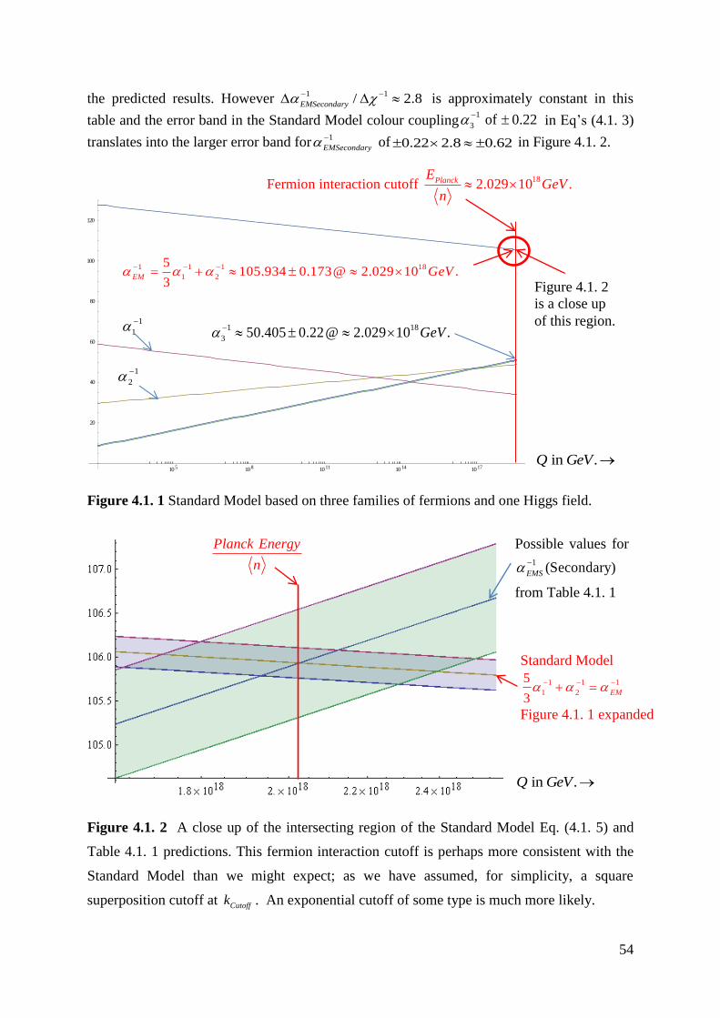
54

the predicted results. However1 1

/ 2.8EMSecondary

is approximately constant in this

table and the error band in the Standard Model colour coupling1

3 of 0.22

in Eq’s (4.1. 3)

translates into the larger error band for1

EMSecondary

of 0.22 2.8 0.62 in Figure 4.1. 2.

Figure 4.1. 1 Standard Model based on three families of fermions and one Higgs field.

Figure 4.1. 2 A close up of the intersecting region of the Standard Model Eq. (4.1. 5) and

Table 4.1. 1 predictions. This fermion interaction cutoff is perhaps more consistent with the

Standard Model than we might expect; as we have assumed, for simplicity, a square

superposition cutoff at Cutoffk . An exponential cutoff of some type is much more likely.

105 108 1011 1014 1017

20

40

60

80

100

120

1 18

350.405 0.22@ 2.029 10 .GeV

1

1

1

2

in .Q GeV

Figure 4.1. 2

is a close up

of this region.

Possible values for

1(Secondary)

EMS

from Table 4.1. 1

18Fermion interaction cutoff 2.029 10 . Planck

EGeV

n

Standard Model

1 1 1

1 2

5

3EM

Figure 4.1. 1 expanded

in .Q GeV

Planck Energy

n

1 1 1 18

1 2

5105.934 0.173@ 2.029 10 .

3EM

GeV

55

4.2 Introducing Gravity into our Equations

4.2.1 Simple square superposition cutoffs

In section 3.2 we looked at single integer n superpositions of nk initially for clarity, and

later found multiple integer n superpositions gave the same results; we will do the same here.

We also found in Eq’s. (3.2. 3) & (3.2. 6) that the integrals for both angular momentum and

rest masses are of similar form. They both ended up including the term

2

0

1

1nk

K

which if nkK cutoff becomes

2

0

1

1

nkK cutoff

nkK

and this is equal to

2

2 2 2

1 1 11

1 1 1 1 / ( ) 1

nk

nk nk nk

K cutoff

K cutoff K cutoff K cutoff

(4.2. 1)

where using Eq. (3.1. 11) the infinitesimal 2 2

0

2 2 2 2

21

( )nk cutoff

m c

K cutoff n k s

(4.2. 2)

For integral or half integral angular momentum precision is required but Eq. (3.2. 6) now

gives us ( )z

TotalL2

0

1 1

2 1 2 1

nkK cutoff

nk

sm sm

K

. So can the effect of gravity increase

our probabilities from dk

sNk

to (1 )dk

sNk

? We will initially address only massive

infinite superpositions where 1N in Eq. (2.2. 4).

The first question we need to address is what is the effective preon mass to be used when

coupling to gravity? In Eq. (3.1. 4) we said the preon rest mass is 0

/ (8 2 )nk

m s for each of

the 8 preons that build a spin ½ particle of rest mass 0m . Now gravity couples to the total

mass including the kinetic energy. It also couples to other terms in Einstein’s energy-

momentum tensor, but we conjecture that in primary interactions such as this (section 1.1.2),

gravitons only couple to the mass/energy, and the equations are consistent only if this is so.

(Sections 6.2.1 & 6.2.2 also discuss this further.)

At the start of the interaction each preon mass is 0

/ (8 2 )nk

m s and after the interaction

(Figure 3.1. 3) it is 2

0(1 ) / (8 2 )

nk nkm s . Let us think semi classically again and see where

it leads us. We have been using magnitudes of velocities as they are the most convenient way

to express our equations even if not the conventional language of quantum mechanics. The

56

interaction with the zero point fields takes the momentum of each preon from zero to

02 / (8 2 )

nk nkm c s (Figure 3.1. 3). While this happens as a quantum step change let us

imagine it as a virtually infinite acceleration from zero velocity to 2

2 / (1 )nk nk

, which is

the relativistic velocity addition (see Figure 3.1. 1) of 2 equal steps of .nk

At the half way

point after one step the velocity is nk (the velocity of the CMF, the preon mass has increased

to0

/ (8 2 ).m s We can imagine this as being like the central point of a quantum interaction.

We will conjecture this midway point preon mass0

/ (8 2 )m s is the mass value that gravity

acts on and we will see that it is indeed the only value that fits all equations. Also it does not

make sense to choose either of the end point masses. We can also get reassurance from the

properties of the Feynman transition amplitude which tells us in Eq. (3.1. 15)

0

0

0

( ) 2

( ) 2f

z

i f nk nk

i nk

p p m

p p m

nk

and the ratio of space to time polarization in the LF is2

.nk

This centre of momentum velocity tells us the key properties of the interaction. We will thus

assume we have 8 preons in each nk of effective gravitational mass

0/ (8 2 )m s with

effective total gravitational mass0

/ 2m s . To put the gravitational constant in the same form

as the other coupling constants we need to divide it by c . The gravitational coupling

amplitude is thus 0

/ (2 )P

m G s c to the gravitational zero point field, where PG is the

primary amplitude for a Planck mass to emit or absorb a graviton. Now this gravitational

amplitude can be regarded as a complex vector just as colour and electromagnetism. We

assumed for simplicity, as they are both spin 1 field particles, that colour and

electromagnetism are parallel. Spin 2 gravity could be at a different complex angle to the

other two. In fact the equations only have the correct properties if gravity is at right angles to

colour and electromagnetism. Putting Primary G SecondaryG G we conjecture that:

0 0

0

/ (2 ) / (2 )

The gravitational coupling

am

plitude

is

/ (2 )

P G S

G

im G s c im G s c

im G s c

(4.2. 3)

Where we have put the secondary gravitational coupling constant to a bare Planck mass sG

in Eq. (4.2. 3) equal to the measured gravitational constant G and temporarily labelled the

ratio between the primary the primary and secondary gravitational constants as G and return

to this in section 6.2.5. So modifying Eq’s. (2.2. 1) to (2.2. 3) by adding Eq. (4.2. 3)

2 2

Q A

2

0 2 4 28 8 / (2 )

.3

EMP Gim G s c sN dk

k rsN k

57

2 2

Q A

2

2 4 28 8 ) (1 )

.3

EMP sN dkk r

sN k

where

2

0

22 (8 8 )

G

EMP

m G

s c

Our previous wavefunctions k required

2 2Q A

2

2 4 28 8 )

3

EMP

k rsN

from Eq. (2.2. 4).

Thus primary graviton interaction can increase the probability of our previous wavefunctions

k by 1 as required to obtain precision in our integrals for / 2 & if .

nkK cutoff

Using Eq.(4.2. 2) now put2 2

0

2

2

0

2 22 22

2

()

1

(8 )8 nk cut

G

EMP off

m G

s

m c

K cutoff snc k

(4.2. 4)

Thus 2

4 (8 8 )

G

EMP

G

c

2

2 2 2( )

cutoff

c

n k

3 2 22

1

( )256(1 )

G

cutoffEMP

G

c n k

2

2

3 2 22

1But and

( )256(1 )

G P

P

cutoffEMP

LGL

c n k

2

2 2

256(1 ) For 1 single integer superpositions

( )

EMP

G

cutoff P

N nn k L

(4.2. 5)

For 1N superpositions k n nk

n

c , we can use the logic of section 3.5.1; replacing 2

nkK

with2

,k

K and 2

n with 2

n in Eq. (4.2. 4), so that Eq. (4.2. 5) becomes

2

2 2

256(1 )For 1 multiple integer superpositions

( )

EMP

G

cutoff P

N nn k L

(4.2. 6)

If we now go back to Eq’s. (2.3. 9) & (2.3. 10) as k the energy squared2 2 2

nk nkE c p

2 2 2n . Again using the logic of section 3.5.1 for multiple integer n superpositions the

expectation value for energy squared as k is 22 22 2 2 2

k kE c n k c p thus

For multiple integer superpositions as , k k

n k E c n kc p (4.2. 7)

58

4.2.2 All N = 1 superpositions cutoff at Planck Energy but interactions at less

It is reasonable to assume that the cutoff superposition energy cannot exceed the Planck

energy PlanckE (at least for square cutoffs) and that this is true for all 1N superpositions.

(Section 6.2.1 discusses N = 2 superposition PlanckE cutoffs.) So for simple square cutoffs:

( )1 multiple integer superpositions cutoff ener gy

k cutoff cutoff PlanckN n E n k c E (4.2. 8)

This can be written as cutoff Planck

Planck

cn k c E

L

For  1 multiple integer superpositions1

         & 1cutoff cutoff P

Planck

n k n k LnL

N (4.2. 9)

1 multiple integer superposition interaction cutoff energy Planck

cutoff

EN n ck

n

(4.2. 10)

Using Eq. (4.2. 10) with Planck energy 191.22 10 .GeV and 6.0135n from Eq.(3.5. 16) for

simple square cutoffs (also see Figure 4.1. 2).

18

Interactions between 1 fermions cutoff @ 2.0288 10 .N GeV (4.2. 11)

From Table 4.3. 1 we see that all other particles such as photons, gluons and gravitons etc.

have 6n and thus higher interaction cutoff energies than fermions ie. 18

2.03 10 .,GeV

but < .P

E Putting 18

2.0288 10 .GeV in the Standard Model equations (4.1. 3) & (4.1. 4).

1 1

1

1 18

1

1

2

1

3

2

@ 2.0288 10 . 34.4179 0.08@ ( )

............................... 48.5707 0.04....................

............................... 50.4053 0.22.....................

5

3EM

GeV k cutoff

1........ 105.934 0.173...................

(4.2. 12)

Real world high energy secondary interactions only involve 1 2 3, & , but spin zero primary

interactions do not involve the weak force. Table 4.1. 1 can thus only predict 1

105.921EM

at the cutoff compared to the Standard Model combination of 1 1

1 2(5 / 3)

1

EM

105.934 0.173 of Eq. (4.2. 12). (See Figure 4.1. 1 & Figure 4.1. 2). Also using Eq’s. (3.3.

3) & (4.2. 12) we get the primary to secondary fundamental coupling ratio C .

1 18

3 Coupling Ratio @ 50.405 0.22 (ie.@ 2.0288 10 .)

C cutoffk GeV

(4.2. 13)

The secondary coupling constants in Eq. (4.2. 12) can be thought of as those to the bare

colour and electromagnetic charges.

59

If we now put Eq. (4.2. 9) into Eq. (4.2. 6) we get 2

2

2 2

256(1 )256(1 )

( )

EMP

G EMP

cutoff Pn k L

From Eq’s.(4.1. 2) and Table 4.3. 1 we find (1 ) 1.115EMP

and Eq.(4.2. 6) becomes

2

256(1.115) 318.3G

(4.2. 14)

Using Eq. (4.2. 3) 318.3G

is the ratio between the primary graviton coupling to bare

preons, and the normal measured gravitational constant (Big G). In other words the primary

graviton coupling to preons is (Primary) (318.3) .G

G (Section 5.1.2, Eq. (5.1. 7)) defines

the secondary graviton coupling between Planck masses G and section 5.3.2, Eq. (5.3. 14)

finds contrary to expectations that 1 / 72.8G

so as in Eq.(6.2. 7) the primary to secondary

graviton coupling ratio is 72.8G

and 318.3 23, 0.8 272 0G

.) When 318.3G

in

Eq.(4.2. 4) the contribution from gravity (the in Eq.(4.2. 4)) cancels any deficit in primary

interactions (the in Eq.(4.2. 4)) if these superpositions cutoff at Planck energy, which we

argue is true for all 1N superpositions. (Sections 6.2 & 6.2.1 discuss 2N superposition

PE cutoffs.) To enable high energy interactions 2N (infinitesimal mass) bosons must also

cutoff at Planck energy just as 1N superpositions do, or as in Eq. (4.2. 10). Figure 4.2. 1

plots radial probabilities for all 3,4,5,6&7n Planck Energy cutoff modes. They are

identical as the radial probability8 2 2 2

( / 9)R

P r Exp n k r , but from Eq. (4.2. 7) 1nk in

each Planck energy mode, so they all have radial probability6 8 2

8.74 10 ( / 9)R

P r Exp r

.

Despite each 3,4,5,6&7n mode having Planck energy the probability in every case of

being inside the Planck region is virtually zero at7

8.9 10

.

Radius in Planck units. Rad

ial

Pro

bab

ilit

y

Planck region

Figure 4.2. 1

All Planck energy n modes look identical

60

4.3 Solving for spin ½, spin 1 and spin 2 superpositions

Superpositions with 2N are covered in section 6.2 but Eq.(4.2. 13) and Eq. (3.3. 22)

extended by keeping N s constant as in Eq. (4.4. 1) allow us to solve various combinations

of spins ½, 1 or 2 and 1N or 2N .

4 4

12

6 6 6 6

12

5 5 5 54 4

( 2) (Sp ( 1) (Spin 1)

or ( 2) (Spin )

( 1) (Spin )

* (1

in 1)

or (

1) (Spin 2)

4 * 2 * (1 *(1

) ) * )

* b b b bb b a a ab b a

N

N

c c c c

N

N

c c

N

c cc c c c

2 / 2 / 50.4053 0.199194C

(4.4. 1)

Starting with spin ½ we can solve this to get 6 6* 0.7254c c as the dominant value.

Putting 6 6* 0.7254c c into Eq.(4.1. 2) or alternatively using Table 4.1. 1

12

6 61.386256 0.1 75.64997258 * 91

EMPc c

(4.4. 2)

From Eq. (2.2. 4) the available 2 2

Q A

2

2 4 28 8 )

3

EMP

k rsN

with probability sN dk

k

where we ignore the infinitesimal factor of (1 ) due to gravitons. And from Eq. (2.3. 12)

2

4 2 4 2

2 2 2 4 2

4

8 8 )*

81 3

* 1367.58 for (spin 1/2 1)

683.79 for (spin 1 1) or (spin 1/2 2)

341.9 for (spin 1 2) or (sp

EMP

n n

n

n n

n k rQ A c c k r

sN

c c n N

N N

N

in 2 1)

170.95 for (spin 2, 2) by extension.

N

N

(4.4. 3)

The same primary electromagnetic coupling EMP builds all fundamental particles, allowing

Eq.(4.4. 3) to be true. Using Eq’s (4.4. 1),(4.4. 3) & * 1n nn

c c we get Table 4.3. 1. We

define the coupling ratio for gravitons 23, 200G

in Eq.(6.2. 7) section 6.2.5, where we

also solve infinitesimal mass graviton superpositions. In Table 4.3. 1 three member

superpositions fit the Standard Model best. In section 4.1 we solved spin ½ superpositions

with a dominant centre mode 6 6*c c that fitted the Standard Model. However when solving

for spins 1 & 2 we must initially comply with Eq. (4.4. 1) which defines interaction

probabilities (see Eq. (3.3. 22) and final paragraph section 3.3.4). We must also comply with

Eq.(4.4. 3) which determines centre or side mode dominance. In this table we have also

included a massive 1N spin 2 graviton type Dark Matter possibility interacting only with

2N spin 2 gravitons. There are other possibilities which we have not included. To this

point this paper has attempted to demonstrate that infinite superpositions can behave as the

Standard Model fundamental particles.

61

The methods used may seem unconventional, but it is important to remember that primary

interactions are very different to secondary interactions (see sections 2.2.2 & 2.2.3).These

methods are however based on simple quantum mechanics and relativity, and there is also

surprising consistency with the Standard Model. If the principles behind the outcomes of

these derivations are at least on the right track and fundamental particles can be built by

borrowing energy and mass from zero point fields then, as we will see in what follows, this

may possibly have some significant and profound consequences.

Mass Type Spin N 3 3*c c

4 4

*c c

5 5

*c c

6 6

*c c

7 7

*c c

Infinitesimal mass gravitons 2 2 0.8346

55.4 10

0.1653

Infinitesimal mass bosons 1 2 0.4847 0.0526 0.4627

Massive (dark matter?) gravitons 2 1 0.4847 0.0526 0.4627

Massive bosons 1 1 0.0134 0.8878 0.0988

Massive fermions ½ 1 0.1305 0.7254 0.1441

Table 4.3. 1 Approximate probabilities for various possible superpositions.

5 The Expanding Universe and General Relativity

5.1 Zero point energy densities are limited

If the fundamental particles can be built from energy borrowed from zero point fields and as

this energy source is limited, (particularly at cosmic wavelengths) there must be implications

for the maximum possible densities of these particles. In section 2.2.3 we discussed how the

preons that build fundamental particles are born from a Higg’s type scalar field with zero

momentum in the laboratory rest frame. In this frame they have an infinite wavelength and

can thus be borrowed from anywhere in the universe. This would suggest that there should be

little effect on localized densities, but possibly on overall average densities in any or all of

these universes. So which fundamental particle is there likely to be most of? Working in

Planck, or natural units with 1G we will temporarily assume the graviton coupling

constant between Planck masses is one. (We will modify this later but it helps to illustrate the

problem.) As an example there are approximately 61

10M Planck masses within the

causally connected or observable universe. They have an average distance between them of

approximately the radius OHR of this region. Thus there should be approximately

2 12210M

virtual gravitons with wavelengths of the order of radius OHR within this same volume. No

other fundamental particle is likely to approach these values, for example the number of

virtual photons of this extreme wavelength is much smaller. (Virtual particles emerging from

the vacuum are covered in section 6.2.2.) If this density of virtual gravitons needs to borrow

more energy from the zero point fields than what is available at these extreme wavelengths

does this somehow control the maximum possible density of a causally connected universe?

62

5.1.1 Virtual Particles and Infinite Superpositions

Looking carefully at Section 3.3 we showed there that, for all interactions between

fundamental particles represented as infinite superpositions, the actual interaction is only

between a single wavenumber k superposition of each particle. We are going to conjecture

that a virtual particle is just such a single member. Only if we actually measure the

properties of real particles do we observe the properties of the full infinite superposition. The

full properties do not exist until measurement, just as in so many other examples in quantum

mechanics. We will use this conjectured virtual property below when looking at the

probability density of virtual gravitons of the maximum possible wavelength. These virtual

gravitons would be a superposition of 3,4,5n modes as in Table 4.3. 1, but of a single

wavenumber k only. Time polarized, or spherically symmetric, versions would be a further

equal (1 / 5) superposition of 2, 1,0, 1, 2m states of the above 3,4,5n mode

superpositions. A spin 2 virtual graviton in an 2m state is simply a superposition of the

three modes 3,4,5n as above but all in an 2m state.

5.1.2 Virtual graviton density at wavenumber k in a causally connected Universe

From here on we will work in natural or Planck units where 1c G .

General Relativity predicts nonlinear fields near black holes, but in the low average densities

of typical universes we can assume approximate linearity. The majority of mass moves

slowly relative to comoving coordinates so we can ignore momentum (i.e. 1) , provided

we limit this analyses to comoving coordinates. Spin 2 gravitons transform as the stress

tensor in contrast to the 4 current Lorentz transformations of spin 1, but, at low mass

velocities the only significant term is the mass density 00T . In comoving coordinates the vast

majority of virtual gravitons will thus be time polarized or spherically symmetric which we

will for simplicity call scalar. We should be able to simply apply the equations in sections 3.4

& 3.5 to spin 2 virtual graviton emissions, as they should apply equally to both spins 1 & 2 at

low mass velocities. (This is not necessarily so near black holes.) We will assume spherically

symmetric 3l wavefunctions emit both spin 1 & 2 scalar virtual bosons, and 3, 2l m states can emit both 1m spin 1 bosons and 2m spin 2 gravitons. Section 3.4 derived

the electrostatic energy between infinite superpositions. In flat space we looked at the

amplitude that each equivalent point charge emits a virtual photon, and then focused on the

interaction terms between them. Thus we can use the same scalar wavefunctions Eq’s. (3.4.

1) for virtual scalar gravitons as we did for virtual scalar photons. Using 1 2( ) * 1( 2 )

1 1 1 2 2 1 2 2* * * * we showed in section 3.4.1 that the interaction term for

virtual photons is

1 2( )

1 2 2 1 1 2

1 2

4* * cos ( )

4

k r rke k r r

r r

(5.1. 1)

63

This equation is strictly true only in flat space but it is still approximately true if the

curvature is small or when 2 / 1m r , which we will assume applies almost everywhere

throughout the universe except in the infinitesimal fraction of space close to black holes. In

both sections 3.4 & 3.5, for simplicity and clarity, we delayed using coupling constants and

emission probabilities in the wavefunctions until necessary. We do the same here. There will

also be some minimum wavenumber k which we call mink where for all min

k k there will be

insufficient zero point energy available. We want Eq. (5.1. 1) to still apply at the maximum

wavelength where min1 / ( 1 / )

OU ObsevableUniversek R R . In Section 6 we find gravitons have an

infinitesimal rest mass 0m of the same order as this minimum wavenumber min

k . At these

extreme k values this rest mass must be included in the wavefunction exponential term. It is

normally irrelevant for infinitesimal masses. Section 6.2 looks at 2N infinitesimal rest

masses finding2

min1

kK . Using Eq.(3.1. 11) with 1c

2 22 min

min 2

0

12

k

s n kK

m and for spin 2 gravitons

2 2

min

0 min2

0

1 or n k

m n km

(5.1. 2)

From Table 4.3. 1 we find

For 2N spin 2 gravitons 3.33n so that 0 min3.33m k (5.1. 3)

This virtual mass 0m increases the E term in / 2E T for a virtual graviton from

E k to 2 2

0E k m when 1c . This reduces the range 1

r T E

over which

it can be found. The exponential decay term in its wavefunction changes from kr

e

to 2 2

0k me

, so we can define a k using Eq. (5.1. 3) such that

22 2 2 2

min min min i

2

m n0 min11.09 and 11.09 3.4 77k k kk k m k k k (5.1. 4)

The normalized virtual graviton wavefunction in Eq. (3.4. 1)

A massless with infinitesim2 2

al become mass 4

s4

kr ikr k r ikrk e k e

r r

(5.1. 5)

Thus the massless interaction term in Eq. (5.1. 1) becomes with this infinitesimal mass 0m

1 2

( )1 2 2 1 1 2

1 2

4* * cos ( )

4

k r rke k r r

r r

(5.1. 6)

Let point P in Figure 5.1. 1 be anywhere in the interior region of a typical universe. Let the

average density be U

(subscript U for homogeneous universe density) Planck masses per

64

unit volume. Consider two spherical shells around point P of radii 1 2

&r r and thicknesses

1 2&dr dr with masses

2

1 1 1 14

U Udm dv r dr &

2

2 2 2 24

U Udm dv r dr .

Now we expect the graviton coupling constant to be 1G

between Planck masses but

because we do not really know this let us define

The Secondary graviton coupling constant between Planck masses G

(5.1. 7)

Section 3.4.1 in Eq. (3.4. 3) used a scalar emission probability (2 / )( / )dk k which becomes

(2 / )( / )G

dk k between Planck masses. (We return to this in section 5.3.2) Now quantum

interactions are instantaneous over all space but distant galaxies recede at light like velocities.

However at the same cosmic time T in all comoving coordinate systems, clocks tick at the

same rate, and a wavenumber k (or frequency) in one comoving coordinate system measures

the same in all comoving coordinate systems. Thus as we integrate over radii 1 2

& 0r r

we can still use the same equations as if the distant galaxies are not moving. (The vast

majority of mass is moving relatively slowly in these comoving coordinate systems and we

return to this important comoving coordinate property in section 5.3.1). Using this new

coupling probability between Planck masses (2 / )( / )G

dk k we can now integrate over both

radii 1 2&r r ; but to avoid counting all pairs of masses 1 2

&dm dm twice, we must divide the

integral by two. The total probability density of virtual gravitons at any point P in the

universe at wavenumber k is using Eq.(5.1. 6)

1 2

1 2

2

( )2 2

1 1 2 2 1 2

1 20

( )2

1 2 1 2

0

2 44 4 cos ( )

2 4

16 cos ( )

k r rU

Gk

k r r

G

G U

kr dr r dr e k r r

r r

kdk r r e k r r

k

Expanding 1 2 1 2 1 2cos ( ) cos cos sin sink r r kr kr kr kr , then using:

2dr

2r

Figure 5.1. 1

1r

1dr

Central point P

65

2 2

2 2 2

0

( ) cos( )

r

r

k krExp k r kr

k k

and 2 2 2

0

2( ) sin

( )

r

r

k krExp k r kr

k k

yields 2 2 2

2

2 2 4

( )16

( )Gk UG

k k kdk

k k k

2

2 2 2

116

( )UG

kdk

k k k

(5.1. 8)

From Eq.(5.1. 4) 2 2 2 2

0 min11.09k k m k k and we can write Eq.(5.1. 8) as

2 2

min2

22 2

min

11.09 116

2 11.09Gk G U

k kdk

k k k

2

4

min

2

22

11.09

2 11.016

9

U

G

x

x xdk

k

where

min

kx

k

2

4

min

2

22

0.3247Wavelength Graviton Probability Density

49.27 11.09

2 11.09

G U

Gk

x

x xk dk

k

2

min min4

mi minn

0.3247Maximum wavelength Probability Density whe 1n U

Gk

G dk

kx

kk

(5.1. 9)

As we think minGK will prove to be a universal constant scalar we will write this as follows.

2

min min min min 4

min

0.3247Maximum wavelength Probability Density where U

Gk

G

Gk GkK dk K

k

(5.1. 10)

5.2 Can we relate all this to General Relativity?

The above assumes a homogeneous universe that is essentially flat on average. At any cosmic

time T it also assumes there is always some value mink where the borrowed energy density

min minGk ZPE E the available zero point energy density min

@ k . It is also in comoving

coordinates. At the same cosmic time T, all comoving observers measure the same

probability density min min minGk G kK dk as in Eq. (5.1. 10). So what happens if we put a small

mass concentration 1m at some point? The gravitons it emits must surely increase the local

density of mink gravitons upsetting the balance between borrowed energy and that available.

However General Relativity tells us that near mass concentrations the metric changes, radial

rulers shrink and local observers measure larger radial lengths. This expands locally

measured volumes lowering their measurement of the background minGk . But clocks

slowdown also, increasing the measured value of mink . Let us look at whether we can relate

these changes in rulers and clocks with the min min minGk G kK dk of Eq. (5.1. 10).

5.2.1 Approximations with possibly important consequences

Let us refer back to Eq. (3.4. 2) and the steps we took in section 3.4.1 to derive it; but now

including 2 2

0 min11.09k k m k k as in Eq.(5.1. 4)

1 2( )

1 2 2 1 1 2

1 2

4* * cos[ ( )]

4

k r rke k r r

r r

(5.2. 1)

66

Central observer

at point P 1

r

Assume that space has to be approximately flat with errors 1/2

1 (1 2 / ) / .m r m r If we

now focus on Figure 3.4. 2 , equation (5.2. 1) is the probability that a virtual graviton of

wavenumber k is at the point P if all other factors are one. Let us now put a mass of 1m

Planck masses at the Source 1 point in Figure 3.4. 2 or as in Figure 5.2. 1.

Also assume that the point P is reasonably close to mass 1m (in relation to the horizon radius)

at distance 1r as in Figure 5.2. 1 and the vast majority of the rest of the mass inside the

causally connected or observable horizon OHR is at various radii r, equal to 2

r of Eq.(5.2. 1)

where 2 1r r r and thus 1

cos[ ( )]k r r cos( )kr . Only under these conditions can we

approximate Eq. (5.2. 1) as

1 2 2 1

1

4* * cos( )

4

k rke kr

r r

(5.2. 2)

As we have assumed average particle velocities are low ( relative to comoving coordinates)

this is a scalar interaction (as in section 3.4.1) and as there are no directional effects we can

consider simple spherical shells of thickness dr and radius r around a central observer at the

point P which have mass 2

4 .U

dm r dr At each radius r the coupling factor

(2 / )( / )dk k we used in Eq. (3.4. 3) using Eq. (5.1. 7) becomes (2 / )( / )G

dk k between

Planck masses and again we use the fact that all instantaneously connected comoving clocks

tick at the same rate.

21 1

2 2Coupling factor 4

U

G Gm mdk dk

dm r drk k

(5.2. 3)

Including this coupling factor in Eq. (5.2. 2)

Spherical shells thickness dr

& mass 2

4U

dm r dr

Mass 1m

r

Radius 1r r

Figure 5.2. 1

67

2 21 1

1 2 2 1

1

1

1

2 2 4( 4 )( * * ) 4 cos( )

4

8 cos( )

k r

U U

k rU

G G

G

m mdk dk kr dr r dr e kr

k k r r

m k dkre kr dr

r k

(5.2. 4)

This is virtual graviton density at point P due to each spherical shell. (Ignoring the relatively

small number of particularly mink gravitons emitted by mass 1

m itself 1 1*

m m , see

addendum 8). Integrating over radius 0r the virtual graviton density at wavenumber k

using Eq’s.(5.1. 4) & (5.2. 4)

1

1 0

2 2

1

2 2 2

1

8cos( )

8 ( )

( )

k rU

G

U

G

G

m k dkre kr dr

r k

m k dk k k

r k k k

(5.2. 5)

Now2 2 2 2 2

0 min11.09k k m k k and if min

k k then 2 2

min min12.09k k and so when min

k k :

1 1

2 2 2

min min1 min min

min 2 2 2

1 min min min

1

min Universe Universe min2

1 min

12.098 (12.09 )

(12.09 )

= ( * + * ) 0.573

U

Gk

U

Gk m

G

m G

k dkm k k

r k k k

mdk

r k

(5.2. 6)

Equation (5.1. 10) suggests min min minGk G kK dk . In comoving coordinates in a metric far

from masses & g , mink has its lowest value. As we approach any mass min

k increases

to mink where we use green double primes when g to avoid confusion with the

min&k k of Eq.(5.1. 4). At a radius r from mass m the Schwarzchild metric is

1/2(1 2 / )m r

for the time and radial terms. Radial rulers shrink and clocks slow, measured

volumes and frequencies both increase locally as 1m

r .Thus using min min minGk G k

K dk

If r m ; min min min

minmin min1 1k

kk dm V V V

r V V

k

k dk

(5.2. 7)

So in this metric the total number of mink gravitons is the original ( )g

minGk of Eq.

(5.1. 10) plus the extra due to a local mass of Eq. (5.2. 6), but we have to divide this number

by the increased volume to get the new density n minmi(1 )

Gk Gk

m

r . Thus using Eq. (5.2. 7)

The new min min m

m

in mi

i minn

n (1 / )1 / (1 / )

Gk Gk Gk Gk

GkGkm r

V V m r

68

2

min min min min(1 / ) (1 2 / ) (if )

Gk Gk Gk Gkm r m r r m

min min

min

21Gk Gk

Gk

m

r

or min

min

2Gk

Gk

m

r

(5.2. 8)

Using Eq’s. (5.1. 9), (5.2. 6) & (5.2. 8) and dropping the now unnecessary subscripts, the

graviton coupling constant G cancels out:

min2

min min

2

minmin4

mi

2

min

n

0.573

2

0.324

1 7

7

. 65

U

Gk

UGk

G

UG

mdk

r k m k m

r rdk

k

(5.2. 9)

(Strictly speaking we should be using minkdk in the top line of this equation but the error is

second order as we are approximating with r m . We will do this more accurately below

for large masses.) For the above to be consistent with General Relativity this suggests that:

“At all points inside the horizon, and at any cosmic time T, the red highlighted part is 2 in

Planck units. This is simply equivalent to putting 2/ 1G c G c ”.

Thus we can say

2

2

min 2

min

(0.8823) 0.8823

Where the parameter is in radians, and is close to 1

The average density of the universe

.

U

OU

OH

kR

k R

(5.2. 10)

Putting Eq. (5.2. 10) the average density U into Eq. (5.1. 10) gives minGk

& minGkK .

2 2

mi

2

min min4

min

min min min min4

min

mi

n

mn

0.3247Maximum Wavelength Graviton Probability Density

0.3247 0.253

Where we label 0.25

(0.8823 )

"The3 a s

U

Gk

Gk Gk

G

G

G

Gk

G

dkk

dk dk K dkk

K

k

k

in

Graviton Constant".

(5.2. 11)

If our conjectures are true, this is the number density of maximum wavelength gravitons

excluding possible effects of virtual particles emerging from the vacuum. In section 6.2.2 we

argue these do not change the minGkK of Eq. (5.2. 11). However minGk

K does depend on the

graviton coupling constant G between Planck masses, but G

cancels out in Eq. (5.2. 9).

It does not affect the allowed universe average density U in Eq. (5.2. 10).

69

5.2.2 The Schwarzchild metric near large masses

At a radius r from a mass m (dropping the now unnecessary suffixes) the Schwarzchild

metric is 1/2

(1 2 / )m r

for the time and radial terms which can be written as

00

2

1 1 1

1 2 1/M

M

rrg

m r g

(5.2. 12)

Velocity M ( 1c ) is that reached by a small mass falling from infinity and

1

M

is the metric

change in clocks and rulers due to mass m . We are using green symbols with the subscript M

for metrics g as we did for mink above. The symbols

1

M

help clarity in what follows.

Using these symbols m

2 2

00

min minin min

mimin n

2 1 1 &

1 2 /

&

M M rr

Gk

M M

Gk M

mg

r m r g

k dkk dk

(5.2. 13)

In sections 5.1.2 & 5.2.1 we approximated in flat space. The wavelength of mink gravitons

span approximately to the horizon. They fill all of space. We can think of the space around

even a large black hole as an infinitesimal bubble on the scale of the observable universe. The

normalizing constant of a mink wavefunction emitted from a localized mass is only altered

very close to this mass. Over the vast majority of space it is unaltered. Only close to this mass

will local observers measure min minMk k due to the change in clocks. There is also a local

dilution of the normalizing constant due to the change in radial rulers. We will consider both

these changes in two steps to help illustrate our argument. Now repeat the derivation of

minGk as in section 5.2.1 but with a large central mass as in Figure 5.2. 1.

At the point P consider Eq. (5.2. 2) 1 2 2

1

1* * cos )4

4(

k rkr

r re

k

.

The red part is the normalizing factor discussed above where we will initially ignore the

dilution due to the local increase in volume. The green &k r kr can be thought of as

invariant phase angles. So if we ignore the dilution factor this equation is unaltered. However

the coupling factor contains all the masses in the universe and the local mass m . But in the

Schwarzchild metric this is the mass dispersed at infinity before it comes together. At a radius

r it is measured as Mm . For the same reasons all the mass in the universe is increased by

the same factor .M

We are left with the factor min

min

2G

dk

k

which is the same as

min

min

min

min

2 2M

M

G Gd k

kk

dk

in the changed metric. So if we ignore the dilution factor and

consider only clock changes Eq. (5.2. 6) becomes, dropping the now uneccesary subscripts

With only time change and no dilution min in

m

2

m2

in

0.573 U

Gk MG

mdk

r k

70

But 2

min

0.8823U

k

from Eq.(5.2. 10) so min m

2

in

2 0.253

Gk GM

mdk

r

Equ’s. (5.2. 11) & (5.2. 13) are min0.253

GGkK and

2 2M

m

r so we finally get

Before dilution of the normalization factor min min

2 2

min

M MGk GkK dk (5.2. 14)

So the total mink graviton density before dilution is the original min min minGk Gk

K dk plus the

extra min min

2 2

min

M MGk GkK dk . So before dilution

min min min min min

2 2 2 2

2

2 2 2

2

2

min min

min min min

(Total)

But

(1 )

(1 )

So undiluted (Total)

11

M M M M

M

M M

Gk Gk Gk Gk

Gk Gk

M

M

M

K dk K dk K dk

K dk

(5.2. 15)

If we now increase the volume to that in the new metric, the new volume is Mrr

g times

the original volume. So in the new metric we must divide this value by M .

In the new metric min min

min min

2

min mimin n M

Gk M

M

Gk

Gk Gk

K dkK dk kK d

(5.2. 16)

If for example 2M

, frequencies are doubled so min min2k k , the number density of

gravitons ( minGk min

2Gk

) is doubled, but so is the measurement of a local small volume

element, which is now 2V . The above equations tell us that the original minGk background

gravitons which occupied one unit of volume is now compressed into 1/2 a unit of volume

and the remaining 3/2 units of volume is taken up by the gravitons due to the central mass.

Figure 5.2. 2 illustrates this. The metric appears to adjust itself so that minGkK (the maximum

wavelength graviton probability constant) is an invariant scalar. (See Figure 5.3. 8 also.)

The background gravitons that originally occupied one

unit of volume are compressed into 1/2 a unit of volume as

number densities are doubled in this new metric.

Figure 5.2. 2 An infinitesimal local volume in a metric where 2Mrr

g .

Measured local volumes double, & 3/2 units of volume

the increased number density equals the extra maximum

wavelength gravitons at that point due to a central mass.

71

5.3 The Expanding Universe

Section 5.1.1 conjectures that virtual gravitons are single wavenumber k members of

superpositions, of width dk . They are thus using Eq. (2.1. 4) wavefunctions k occurring

with probability /sN dk k , but we have aready included the factors /dk k in deriving Eq’s.

(5.1. 9), (5.2. 6) & (5.2. 11). The number density of k wavefunctions is simply

4k Gk Gk

sN for spin 2 & 2N gravitons. To get the number density of gravitons at

any wavenumber k we can rewite Eq. (5.1. 9) using Eq.(5.2. 10) for 2 4

min/

Uk & Eq.(5.2. 11)

2

4

min

2 2

2 22 2

49.27 11.09 49.27 11.09

2 1

0.32470.

12

.09 2 11.0953U

Gk

G

G

xdk dk

x

x xk xx

2

22

min

49.27 11.09 where

2 11.090.2534 4

k Gk Gk G

x kN

xk x

xs d

k

(5.3. 1)

The blue part of Eq. (5.3. 1) is one when min/ 1k k x .

From Eq.(3.2. 1) the vacuum debt for a superposition is 2

( ) .k k

debt n p k

Using Eq’s. (3.1. 11), (3.1. 12) & (3.2. 10)

2

2

21

k

k

k

K

K

.

0

2 spin 2For k

n kK

mN and from Eq. (5.1. 3) 0 min

3.33m k from which we can show

2 2

2

2 2 2

n minmi

where 1

k

k x

k k kx

kx

.

From Table 4.3. 1 3.33n for gravitons. Each wavefunction k borrows from the zero

point fields2

2

2

(3.33)

1k

xn

x

wavenumber k quanta. The quanta density required @k by

gravitons is:

2 2

222

2

22

min

@

@ min min

2min

49.27 11.09

1 2 11.09

98.54 11.09

(3.33) 0.253

1.68 & whe 1( 1) 2 11.09

4

n

8

1 .6

Quanta k G

Qk G

Quanta k Qk G

x x

x x x

x x kx

dk

xdk

dk

kx

(5.3. 2)

But the density of zero point modes available min@ k is

2 2

min/k dk (ignoring some small

factors). Even if 1G

this is too small by about2 2

min1/

OHk R . However the area of the

causally connected horizon 2

4OH

R suggests possible connections with Holographic horizons

and the AdS/CFT correspondence [14].

72

5.3.1 Holographic horizons and red shifted Planck scale zero point modes

Malcadena proposed AntiDesitter or Hyperbolic spacetime where Planck modes on a 2D

horizon are infinitely (almost) redshifted at the origin by an (almost) infinite change in the

metric. In contrast we have assumed flat space on average to the horizon. In section 2.2.3 we

defined a rest frame in which zero momentum preons with infinite wavelength build infinite

superpositions. If we also have a spherical horizon with Planck scale modes, but here

receding locally at the velocity of light, these Planck modes can be absorbed by infinite

wavelength preons (from that receding horizon) and red shifted in a radially focussed manner

inwards. We will argue in what follows, that at the centre where the infinite superpositions

are built, approximately 1/6 of these Planck modes can be absorbed from that horizon with

wavelengths of the order of the horizon radius. This potential possibility only exists because

zero momentum preons have an infinite wavelength. If any source of radiation recedes at

velocity /v c the frequency/wavenumber reduces as (1 )observer source

k k where2 1/2

(1 ) . In the extreme relativistic limit 1 & we can put1 .

2

2 2

Putting 1 implies 1 and 1 2

1

1

2 and 1 / 2

Thus

 

(1 )2 22

Observer

Source

k

k

(5.3. 3)

There is always some rest frame travelling at nearly light velocity that can redshift Planck

energy modes into a min1 /

OHk R mode and also many other frames travelling at various

lower velocities that can redshift Planck energy modes into any mink k mode . This is

special relativity applying locally. But in sections 5.1.2 & 5.2.1 we used the fact that clocks

in comoving coordinates tick at the same rate. So how does Eq.(5.3. 3) help? Space between

comoving galaxies expands with cosmic or proper time t and is called the scale factor ( )a t . It

is normally expressed as ( )p

a t t .

Thus 1

( )p

a t pt

and the Hubble parameter( )

( )( )

a t pH t

a t t

(5.3. 4)

Writing the present scale factor normalized to one so that ( ) 1a T implies ( ) /p P

a t t T , we

can get the causally connected horizon radius and the horizon velocity V. Using Eq.(5.3. 4)

0 0

The horizon radius only when is constant.( ) 1

T T

p

OH p

dt dt TR T p

a t t p

(5.3. 5)

1

0

The horizon velocity ( ) 1

But is the current Hubble constant so horizon velocity 1 ( )

T p

p pOH OH

OHp p p

OH

dR Rd dt T pV T pT R

dT dT t T T T

pV H T R

T

(5.3. 6)

73

Now the receding velocity of a comoving galaxy on the horizon is ( )OH

V H T R and thus

from Eq.(5.3. 6) the horizon velocity is always 1V V . In other words the horizon is

moving at light velocity relative to comoving coordinates instantaneously on the horizon as

measured by a central observer. Now clocks tick at the same rate in all comoving galaxies but

clocks moving at almost the horizon light velocity (relative to comoving coordinates

instantaneously on the horizon) will tick extremely slowly or as 1/ from Eq.(5.3. 3) as

special relativity applies locally in this case. Thus Planck modes on the receding horizon will

obey Eq’s.(5.3. 3) as seen in all comoving coordinates. Let us now imagine an infinity of

frames all travelling at various relativistic velocities relative to comoving coordinates

instantaneously on the horizon and radially as seen by central observers. We can think of

these as spherical shells on the horizon all of one Planck length thickness as measured by

observers moving radially with them. Transverse dimensions do not change for all radially

moving observers and the effective surface area of all these shells is2

4OH

R . The internal

volume of all these shells as measured in rest frames by observers moving radially with them

as each of these observers measures their thickness as one Planck length is

2 2Rest frame internal shell volume 4 4

OH OHV R R R (5.3. 7)

We want the zero point quanta available where these quanta have Planck energy E lasting

for Planck time T such that / 2E T . Before redshifting a single zero point quanta

thus has Planck energy (temporarily using a single primed k that is not the k of Eq. (5.1. 4))

where 1k before redshifting and k after redshifting. The density of Planck energy zero

point modes in this shell is 2 2

/k dk and at energy / 2k per mode this is equivalent to

2

22

k dk

quanta, which we will write as zero point quanta density

3

22

dk

k

k

.

(5.3. 8)

Now at Planck energy 1k and we are redshifting to k where from Eq’s.(5.3. 3)

/ 2k k & / 2dk dk . Thus / /dk k dk k . As 1k Eq. (5.3. 8) becomes

3

2 2

1 1Planck Energy Zero Point Quanta Density before redshifting

2 2

dk dk

k k

(5.3. 9)

Now multiply density by volume ie. Eq’s. (5.3. 7) & (5.3. 9) to get the total Planck energy

zero point quanta inside the rest frame shell as 2

2

1

24

OH

dR

k

k . Two thirds of these quanta

are transverse and one third radial so only 1/ 6 of these quanta are available for redshifting

radially inwards. Using Eq.(5.2. 10): After redshifting to wavenumber k these quanta have

radius min min

min

1 1 OH

C

Rk kR

k k k k

and thus occupy spherical volume

33

min

3

4

3

OHR k

Vk

.

74

Again using min OHk R the effective quanta density becomes

3 23

2 min

3

min m

2 2

@ 2 2

3

in

2

1 3 where

44

2 4 46

1Quanta H

OH

k O

kk kx x

R

dkR

kdk k

kk kd

These quanta are half scalar and half the vector required to build infinite superpositions.

Density of vector quanta available after redshifting 2

2

28

kdkx

(5.3. 10)

Now an observer at the centre of all this sees space being added inside the horizon at the rate

of the horizon velocity 1 ( )OH

V H T R as in Eq. (5.3. 6). We will conjecture that the space

added in one unit of Planck time inside the expanding horizon also creates the source of these

zero point quanta that we can borrow. Thus Eq. (5.3. 10) becomes

222

2

2 2

min

(1 )Density of vector quanta availa ble

8 8

OH

k

H RV kdk x dk

k

(5.3. 11)

5.3.2 Plotting available and required zero point quanta

Figure 5.3. 1 plots Eq’s. (5.3. 2) & (5.3. 11) as a function of min/x k k . This plot always

looks the same. At all cosmic times T and in any metric, only the value of mink changes.

It also only works in a continually expanding universe. When mink k we can equate them:

2

min2 min min min

min mi

2

n

Quanta required 1.68

Where 1.68 is the "Quanta requ

Quanta avai

ired @ Consta

la

nt "

ble =8

& 132.65

G Qk

Qk G G

dk K dk

K

dk

k

V

V

(5.3. 12)

Equation (5.2. 10)

2

2the average density of the 0.univ 8823erse

U

OHR

allows us to solve

the present value of min OHk R . Using the 9 year WMAP (March 2013) data for Baryonic

Figure 5.3. 1

Quanta available

Quanta required

min

kx

k

mink

75

and Dark Matter density and radius 61

2.7 10OH

R Planck lengths ( 946 10 light years)

puts2

0.37U OH

R in Planck units. Thus2 2

0.8823 0.37U OH

R yields

The current value for min0.65

OHk R (5.3. 13)

Figure 5.3. 2 Plots2 2

0.8823U OH

R

Figure 5.3. 7 plots 0.83 ( 0.24 )Exp t from Eq.(5.3. 20) out to 10 times the current age of

the universe showing the exponential decrease with time. The current Horizon Hubble

velocity 1 ( ) 4.35OH

V H T R and putting this and 0.65 into Eq. (5.3. 12) we can solve

the approximate graviton coupling constant G .

2

1

132.65 72.8G

V

(5.3. 14)

The actual value for G is less important than the form of this equation as provided Eq. (5.2.

10) 2 2

0.8823U OH

R is true (or in other words all comoving observers measure the

maximum wavelength graviton probability density minGkK as in Eq. (5.2. 11) GR is still true

locally, regardless of graviton coupling G . The normal gravitational constant (big) G is

directly related to the metric change of GR, and if GR is true locally then G will not change,

as it is independent of graviton coupling G . Because Eq. (5.3. 14) depends on the actual

present values for &V it must be approximate. The above analysis is based on a receding

horizon source of cosmic wavelength quanta that can only be borrowed if preons are born

with infinite wavelength. But as we will see, exponential expansion seems to follow naturally

from Eq. (5.3. 14). It also strongly suggests that if fundamental particles are in fact built from

infinite superpositions that borrow quanta from zero point vector fields, then graviton

coupling G between Planck masses must be much less than 1. So are there possible

consequences of this?

0.2 0.4 0.6 0.8

0.1

0.2

0.3

0.4

0.5

0.6

2

U OHR WMAP value

20.37

U OHR

Big Bang

Future

min radians

OHk R

Currently 0.65

76

5.3.3 Possible consequences of a small gravitational coupling constant.

In quantum mechanics, forces between charged particles are due to the exchange of virtual

bosons. All scattering crossections are calculated from the exchanged 4 momenum of these

bosons. General Relativity suggests that the forces of gravity are fictitious and only seem real

due to the change of the metric. This paper proposes that the change in the metric around

mass concentrations is consistent with keeping the “ mink Graviton Constant minGk

K ” of Eq.

(5.2. 11) invariant. These changes in the metric are about 70 times greater than the coupling

constant suggests. We are suggesting in this paper that spin 2 gravitons only cause changes in

the metric by the need to keep minGk at its appropriate value. The attempts to develop a

quantum field theory for gravitons have difficulty with the infinities at Planck energies that

are not renormalizable. They assume a gravitational coupling constant of one between Planck

masses. This could change if this coupling constant is in fact about 70 times smaller, as

Planck energy gravitons would no longer automatically form Black holes. However it may be

irrelevant if, as Einstein believed, gravity is not due to exchanged 4 momentum.

5.3.4 A possible exponential expansion solution and scale factors

Let the scale factor be a then density3

1

a and Eq. (5.2. 10) tells us the average density of

the universe

2

20.8823

U

OHR

so that

2

2 3

1U

OH

KR a

where 0.8823K is a constant.

Thus 3 2 2 2/3 2/3

a KR a K R where OH

R R (5.3. 15)

The Hubble parameter H is

1/3 2/3 2/3 5/3

2/3 2/3 2/3 2/3

(2 / 3) (2 / 3) 2 1 1

3

dR dK R K Ra dR ddt dtHa K R K R R dt dt

2 Thus the Hubble Horizon velocity @ is

3OH

dR RR V H R

dt

d

dt

(5.3. 16)

We can also write Eq.(5.3. 14) 2164 a constant

GV , hence

22 0dV d V .

Thus 1

2

1dV

V dT

d

dT

and Eq. (5.3. 6) tells us that the Horizon velocity OHdR dR

Vdt dt

.

Equation (5.3. 6) also tells us that 1V H R V so we can write Eq. (5.3. 16) as

2 2

3( 1) 22

d

d

R R dVV

V ttV

d

3

R dVV

V dt ( 3)

dV VV

dt R

(5.3. 17)

77

We will look for an exponential increase of the horizon velocity so / 0dV dt and 3 .V

Let us try first a simple 3 ( )V Exp bt with 3V for all values of & 0b t .

Also simply put 0 0

3 ( )t t

R Vdt Exp bt dt thus 3[ ( ) 1]Exp bt

Rb

.

Putting this value for R plus 3 ( )V Exp bt & 3 3[ ( ) 1]V Exp bt into Eq. (5.3. 17)

( 3) 3 ( ) 3[ ( ) 31]3[ ( ) 1]

( )V b

V Exp bt Exp btR Exp b

dVbExp bt

d tt

.

But 3 ( )V Exp bt and again 3 ( ) 3 ( )dV d

Exp bt bExp btdt dt

. Thus Eq’s. (5.2. 10) & (5.3. 14)

are consistent with 3 ( )V Exp bt for positive b regardless of the value of graviton coupling G

A possible expansion solution is 3 ( )V Exp bt & 3[ ( ) 1]Exp bt

Rb

, 0.b

(5.3. 18)

But is this consistent with the local special relativity requirement for OHR ? In other words

does0

3[ ( ) 1]@ time ( )

( )

T dt Exp bTR T a T

a t b

? Now Eq. (5.3. 15) tells us the scale factor

3 2 2 2/3 2/3a KR a K R

but Eq.(5.3. 14) says2

1/V so the scale factor1/3 2/3

.a V R

From Eq. (5.3. 18), ignoring the constant factors 3 & b, ( )V Exp bt & ( ) 1R Exp bt

1/3 2/3

0

1/3 2/3

/3 2 3

0

1 /

The scale factor ( ) ( ) [ ( ) 1]

Thus ( )

=( ) [ ( ) 1]

3[ ( ) 1]

( )

( ) [ ( ) 1]

T

T

a t Exp b

a T

Exp bT E

t Exp bt

dtR

a t

dt

Exp bt Exp bt

Exp b

b

b

xp T

T

5.3. 19)

And Eq. (5.3. 18) appears to be a consistent exponential expansion for both V and R.

From Eq.(5.3. 14) we showed 1

2

1dV

V dT

d

dT

. Using Eq. (5.3. 18) 3 ( )V Exp bt &

3 ( )dV

bExp btdt

implies ( / 2)K Exp bt . The current value of 0.65 from Eq.(5.3.

13) and our best guess of 0.48b from Figure 5.3. 3 yields

min0.83 ( 0.24 ) in radians

OHk R Exp t (5.3. 20)

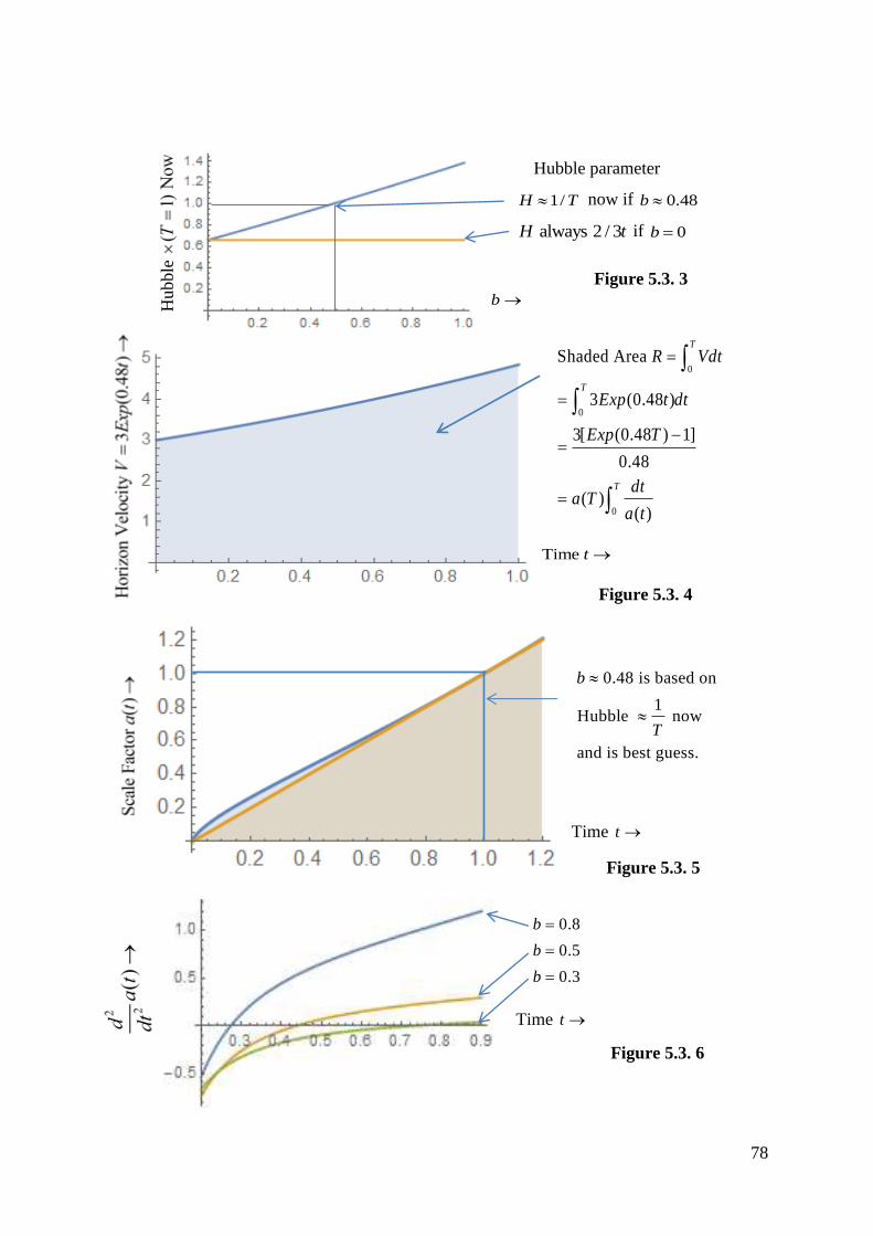
78

Time t

0

0

0

Shaded Area

3 (0.48 )

3[ (0.48 ) 1]

0.48

( )( )

T

T

T

R Vdt

Exp t dt

Exp T

dta T

a t

Figure 5.3. 4

Time t

Figure 5.3. 5

0.48 is based on

1Hubble now

and is best guess.

b

T

Time t

0.8

0.5

0.3

b

b

b

Figure 5.3. 6

Hubble

Figure 5.3. 3

b

Hubble parameter

1/H T now if 0.48b

always 2 / 3H t if 0b

79

5.3.5 Possible values for b and plotting scale factors

This simple exponential expansion starting at the Big Bang is very different to current

cosmology models keeping the Hubble parameter / 2 / 3H a a t constant (if 1 ) until

Dark Energy starts to take effect. A continuous exponential expansion could well lead to

slightly different values for the radius OHR and also possibly the age 9

13.8 10T years.

Current cosmology models put the Hubble parameter as / 1/H a a T at present (based on 9

13.8 10T years). It also simplifies the plots above if we put9

13.8 10 years 1T with

OHR or radius R becoming multiples of 1T . Using Eq. (5.3. 6) 1 ( )V H T R , Figure 5.3.

3 plots the Hubble parameter by time ( 1)T now as a function of the exponential time

coefficient b showing if 0b that always 2 / (3 )H t as in current cosmology at critical

density with no dark energy. Also if 1/H T now the best guess is 0.48b . This yields

3.85R T or 15% greater than current cosmology. Figure 5.3. 4 plots horizon velocity &

Figure 5.3. 5 the scale factor based on 0.48b , but of course the actual value of b or rate of

change with time must be in agreement with the redshifts currently observed when looking

back towards the big bang. These could well change b and radius R. Figure 5.3. 6 plots the

transition to positive acceleration of the scale factor showing the effect of changing the value

of b. Figure 5.3. 7 plots Eq.(5.3. 20) min0.83 ( 0.24 )

OHk R Exp t out to 10 T.

5.3.6 An infinitesimal change to General Relativity effective at Cosmic scale

Section 5 is based on energy in the zero point fields being limited. We argued that uniform

mass density throughout the cosmos has probability density minGk as in Eq. (5.2. 11). At this

probability density the zero point quanta density available equals that required. To maintain

this required balance (see Figure 5.3. 1) we argued that around any mass concentration the

curvature of space expands space locally so as to keep min0.253

GGkK as in Eq. (5.2. 11)

constant at all points. In other words our conjecture only works if the local curvature of space

depends on the difference between the local mass density and the uniform background.

Compared to General Relativity this is an infinitesimal change except at cosmic scale. GR

says the curvature of space depends on local mass density whereas we argue that it depends

on the difference between local mass density and the average background (only a few

2 4 6 8 10

0.2

0.4

0.6

0.8

Figure 5.3. 7

Cosmic time t

0.65 radians now

Current time 1t

Big Bang

80

hydrogen atoms per cubic metre). This automatically guarantees the universe to be flat on

average. All our aguments in Section 5 start with flat space on average. The equations of GR

would look almost identical except the Energy Momentum Tensor T in comoving

coordinates requires 00T the mass/energy density to change from to U

where the

density of the universe U is as in Eq. (5.2. 10).

00 In comoving cordinates changes from to in the Energy Momentum Tensor

UT T

(5.3. 21)

5.3.7 Non comoving coordinates in Minkowski spacetime where g .

To this point everything we have looked at has been in comoving coordinates. Velocities

relative to comoving coordinates are usually referred to as peculiar velocities, so, does what

we are saying above still apply in such non comoving coordinates? In section 5.1.2 we said

that spin 1 sources are 4 currents, but spin 2 graviton sources are the stress tensor. We have

also been saying up to here that the background mink gravitons are spherically symmetric or

time polarized in comoving coordinates. We are going to conjecture that in non rotating

Minkowski spacetime they are always time polarized, regardless of peculiar velocities. This

may seem impossible, as we would intuitively expect something to not remain spherically

symmetric if we move relative to it. But we are not talking about real particles; we are talking

about virtual spin 2 gravitons. We cannot see them, or detect them directly in any way, only

their consequences. We can calculate amplitudes and probabilities for their presence only. So

let us look again at these background mink graviton amplitudes and probabilities. We found in

Equ’s. (5.1. 10) & (5.2. 11) the probability density of background mink virtual gravitons

2

Universe Universe min min min min 4

min

0.3247* where U

Gk Gk Gk

GK dk Kk

in comoving coordinates.

If we move relative to this at peculiar velocity P , measured volumes shrink as

1 2 1/2(1 )

P P

and all comoving mass increases as 2 1/2

(1 )P P

. (We will use red

symbols with the subscript P, and triple primes for wavenumber mink for peculiar velocities, to

distinguish them from metric changes where we used green and a double primed mink .) Thus

2

U P U .The minimum wavenumber min

k has its lowest value in comoving coordinates (at

least far from mass concentrations where g ) but at peculiar velocity P , mi minn P

k k .

2 4

4 4

2 2

min4 4

min mimi nn

and is invariant.U UU P

P

Gkkk

Kk

min min minGk GkK dk is always true in non comoving coordinates if g

(5.3. 22)

81

5.3.8 Non comoving coordinates when g .

Starting with Eq. (5.1. 10) min min minGk GkK dk we have just shown that this equation remains

true at any peculiar velocity P in flat spacetime. All that happens is that the values of min

k ,

mindk & min min minGk Gk

K dk all increase as 2 1/2

(1 )P P

. In other words the probability

of finding a mink graviton is always proportional to whatever the value min

k & mindk is. Also the

amplitude to find a mink graviton is always proportional to either

mink or

mindk . We have

shown in sections 5.1 & 5.2 that around mass concentrations in comoving coordinates, the

mink gravitons are comprised of the background due to the universe plus the interaction

between the local mass and the universe as in Figure 5.2. 2. This background mink graviton

probability, regardless of the local metric, is always proportional to whatever the local value

mink & min

dk is. Amplitudes are also always proportional to local values of min

k or min

dk .

minAmplitude (due to rest of universe)

Gk or Universe min

allways dk (5.3. 23)

As in Figure 5.2. 1 the probability for a small mass m to emit a mink graviton is

2 min

min

2G

dkm

k

.

The normalized wavefunction is min2min min min

2 2 2

2 2 2 3.477

4 4 4

k rk k ke

r r r

where we are using Eq.

(5.1. 4) min min3.477k k and min

0k r . Thus we can say that the:

2

min

minmin min

2 2

min

3.4773.4772Amplitude (due to small mas

2s

2

4 )

G Gk

Gdkdk k m

mk r r

m

(5.3. 24)

min

2

3.4772=

4

m

Gdkm

r

is allways min

2mdk

r

The interaction between this small mass and the rest of the universe is

Universe Universe mimin m nminn i

2 + is allw* * ays

2Gk m m

m mdk

rddk k

r .

We have shown previously that minGkK is the proportionality constant. So regardless of

peculiar velocities

Universe Univmin min merse in + is allways

2* *

mG Gmk k

mK dk

r

(5.3. 25)

Thus Universe Universemin* * +

m mGk is always proportional to min

dk and at peculiar

velocity P ; mi minn P

k k & min minPkdk d . So both min min

&Gk Gk

increase as P and their

ratio does not change. The logic of our aguments is not affected by peculiar velocities. The

same is true for large masses moving at peculiar velocities. In a metric M as in section 5.2.2

(using four blue primes for combined peculiar velocity and metric changes) min minMPk k

82

and n mimi nMPd kk d . Both min min

&Gk Gk

increase as P

M and again their ratio does not

change. All the arguments we used in section 5.2.2 do not change and Equ’s. (5.2. 14), (5.2.

15) & (5.2. 16) still apply in non comoving coordinates providing M is the velocity reached

by a small test mass falling from infinity in the same rest frame as the mass concentration m

moving at peculiar velocity P . We can think of min

0.253GGk

K as a constant scalar

throughout the universe representing the Probability Density of finding a minimum

wavenumber min minMPk k virtual graviton at all points of spacetime. Near mass

concentrations the metric changes. Local clock rates change and so does the measurement of

mink , but not the scalar minGk

K . Locally measured infinitesimal volumes increase to

accommodate the extra locally emitted maximum wavelength gravitons keeping the scalar of

probability density constant. We argue that General Relativity is consistent with this.

If we think of the mass in the universe as a dust of density U essentially at rest in comoving

coordinates we can define a tensor (Background)T . In comoving coordinates

(Background)T has only one non zero term 00(Background)

UT . In any other coordinates

this same (Background)T tensor is transformed by the usual tensor transformations that

apply in GR. If these coordinates move at peculiar velocity P then

2

00(Background)

P UT

2

00(Background)

PT . This all suggests the infinitesimally modified Einstein field equations

4

1 8(Background)

2

GG R g R T T

c

(5.3. 26)

We argue that Eq.(5.3. 26) is consistent with keeping the scalar min0.253

GGkK constant

throughout all spacetime as in Figure 5.3. 8. This infinitesimal modification is only relevant

in the extreme case as T approaches (Background)T . Far from mass concentrations

(Background)T T . Space curvature is, in these remote voids, somewhere between

slightly negative and zero, but the causally connected universe is flat on average regardless of

the value of .

62

min10k

now

At any cosmic time T in any coordinates, and in any metric,

in the infinitesimal band mindk , min min minGk Gk

K dk is always

true. minGkK is a constant scalar, but the measurement of min

k

depends on both local metric clockrates and cosmic time T .

Figure 5.3. 8

minGk

G

K

mink

min0.1 0.25k

very approximately

@ the Big Bang

Future

Past

83

If there is no inflation, in comoving coordinates, at the Big Bang or slightly after, mink starts at

just under one and is always close to the inverse of the causally connected horizon radius. It

is also thus close to the inverse of cosmic time T as in Figure 5.3. 8. It is always at its

minimum far from mass concentrations, but increases with the slower clock rates in the local

metric around mass concentrations. The above arguments are only true if the determinant of

the metric 1g , ignoring the 2 2&sinr factors, in particular 00

1.rr

g g We have also

ignored angular momentum which will change this. We have only considered the gravitons

interacting between a local mass and the rest of the universe and ignored the relatively small

emission of gravitons by the mass itself *m m

. This effect and angular momrntum are

addressed in Part II of this paper. See Addendum 8.

5.3.9 Is Inflation really necessary in this proposed scenario?

There are two main reasons, usually given, for why inflation is necessary:

(a) The average flatness of space.

(b) The almost uniform temperature of the cosmic microwave background from regions that

were initially out of causal contact.

If we put (Local) (Background)T T in Eq. (5.3. 26) the right hand side is identically zero,

and 1

02

G R g R on average throughout all space. The average curvature of all

space must be zero and space is compelled to be flat on average.

In section 5.3.4 we found that space has to expand exponentially as in Eq.(5.3. 18) and

plotted in Figure 5.3. 4. The actual value of the constant b in 3 ( )V Exp bt has to fit

experimental observations. But if it is some fundamental constant, which does not seem

unreasonable, it must be the same for all comoving observers. If this is so the physics is

identical for all such observers regardless of whether they are in causal contact. Provided we

can assume identical starting points everywhere, of say the Planck temperature at cosmic time

0T , then apart from quantum fluctuations, the average background temperature should be

some function of cosmic time T for all comoving observers, or at least up to the time the

universe became transparent. The physics controlling this should be identical in each

comoving frame. Causal contact should not be essential for this. Inflation only guarantees

that the starting temperature is uniform everywhere when it stops at approximately 0.T It

also has to assume identical physics everywhere from 0T for about the first 375,000 years,

or until the universe is transparent. This is virtually identical to what we are proposing in the

scenario in this paper.

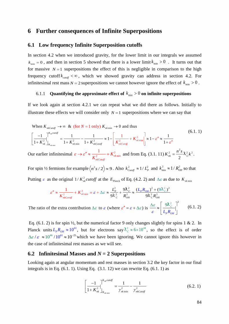
84

6 Further consequences of Infinite Superpositions

6.1 Low frequency Infinite Superposition cutoffs

In section 4.2 when we introduced gravity, for the lower limit in our integrals we assumed

min0k , and then in section 5 showed that there is a lower limit min

0k . It turns out that

for massive 1N superpositions the effect of this is negligible in comparison to the high

frequency cutoff cutoffk , which we showed gravity can address in section 4.2. For

infinitesimal rest mass 2N superpositions we cannot however ignore the effect of min0k .

6.1.1 Quantifying the approximate effect of min0k on infinite superpositions

If we look again at section 4.2.1 we can repeat what we did there as follows. Initially to

illustrate these effects we will consider only 1N superpositions where we can say that

min

min

2

m2 2 2

min

in2

When & 0 and thus

1 1 1 11 1

1 1 1

(for

1

1 only)

1nk

nk

nkCutoff nk

K c

nk

nkCuto

utoff

nk nk nkCutoff ffK

NK K

K K KK

K

(6.1. 1)

Our earlier infinitesimal 2

min2

1nk

nkCutoff

KK

and from Eq. (3.1. 11)2

2 2 2

2nk C

n sK k .

For spin ½ fermions for example 2/ 2 9n s . Also

2 21/

Cutoff Pk L and

2 2

min1/

OHk R so that

Putting as the original 2

1/nk

K cutoff at the PlanckE of Eq. (4.2. 2) and as due to minnk

K

2 2 22

2 2 2 2

2

2

min2

9 ( ) ( )

9 9

91CP

C O

P

nk

nkCutoff H

C

C

OH

H O

L RL

R RK

K

22

The ratio of the extra contribut to (where ) n i9

io s P

C

OHL R

(6.1. 2)

Eq. (6.1. 2) is for spin ½, but the numerical factor 9 only changes slightly for spins 1 & 2. In

Planck units61

10P OH

L R , but for electrons say2 44

6 10C , so the effect is of order

4 56 26 1/ /10 10 10

which we have been ignoring. We cannot ignore this however in

the case of infinitesimal rest masses as we will see.

6.2 Infinitesimal Masses and N = 2 Superpositions

Looking again at angular momentum and rest masses in section 3.2 the key factor in our final

integrals is in Eq. (6.1. 1). Using Eq. (3.1. 12) we can rewrite Eq. (6.1. 1) as

min

2 2 2

min

1 1 1

1

nk

nk

K cutoff

nk nk nkCutoffKK

(6.2. 1)

85

With massive 1N superpositions as above the difference between 2

min& 1

nk is vanishingly

small, i.e.2

min( 1) 1/

nk and as in section 6.1.1 this first term is of much less significance

than the2

nkCutoff term. Now define an approximate equality between

2

min&

kN using Eq.

(3.1. 12) as follows

2 2

min min1

k kN K

(6.2. 2)

In section 3.2 we derived angular momentum and rest masses for only massive or what we

called 1N particles. To get integral angular momentum we had to assume in deriving Eq.

(3.2. 6) that the minimum value of min or 0

nk nkK K . For massive 1N particles such as the

fermions the error in this assumption (as in section 6.1.1) is 2510

times smaller than ,

which for an electron is already 4510

due to the high frequency cutoff @ 18.3110 .GeV

(We allowed for this 4510

when we included gravity in section 4.2.) From section 6.1.1

above we approximated2 2 2

min as 9 /

nk C OHK R for a spin ½ fermion. So we can express Eq. (6.2.

2) in terms of this approximation for fermions with non infinitesimal mass

2 2

2

2

min 2 2

77

2

9 91 1 as

9For example an electron has 10

0

C

O

C C

k

OH OH

H

NR R

R

(6.2. 3)

For the massive particles it appears we can safely say that 1N . Even if neutrino masses

were as low as4

10 eV

then 592

min1 10 .

k

If the mass is too small however Eq. (6.2. 1)

tells us we cannot get the correct angular momentum unless something else changes.

Infinitesimal increases above 1 of the order of 50

10

or so can be handled perhaps by a

small change in the actual high frequency cutoff details, but this probably does not allow

massive particles to be much less than sub micro electron volts. So if massive particles are a

group with 1N , then it would not seem unreasonable to imagine there could possibly be

another group with 2

min2 1

kN K implying that

2

min1.

kK Repeating the derivation

of Eq. (3.2. 6) but with 2

min2 1

kN K and for clarity and simplicity let cutoffnk

K .

min min

2

2 2 2

2

min

1( ) ( 2)

(1 ) 1

1 1( ) as pr

2eviously.

1 ( ) 2

nk nk

nk nk

z

nk nk nkK K

z

nk

K dKTotal s N m sm

K K K

smTotal s

K Nsm m

L

L

(6.2. 4)

Provided we have doubled the probability of superpositions as in Eq. (2.1. 4) from

1( ) /Ns dk k to 2( ) /Ns dk k , the final angular momentum results in Eq’s. (3.2. 6) &

86

(6.2. 4) are identical. The same is true for rest mass calculations. For multiple integer n

infinite superpositions if 2N then the expectation value2

min1

kK .

We thus conjecture that all 2N infinite superpositions have2

min1

kK .

From Table 4.3. 1

2N infinitesimal rest mass spin 1 superpositions have 3.98n

2N infinitesimal rest mass spin 2 superpositions have 3.33n

Using Eq’s. (3.1. 11) and Eq.(5.2. 10).

2

2 2 2 2

min min

2

m

2 2

min

in

15.82 or 0.355 for Spin 1

2 2

11.09 2

1

1 or 0.300 for Spin 2 2

OH

C C C

OH

C C

k

n s Rk k

Rk

K

(6.2. 5)

Using the value for 0.65 from Eq. (5.3. 13) based on WMAP data which also puts

the horizon radius at 946 10 light years

612.7 10

OHR Planck lengths.

Spin n Compton Wavelength c Infinitesimal Rest Mass

1 3.98 0.55OH

R 348.3 10 .eV

2 3.33 0.46OH

R 349.8 10 .eV

Table 6.2 1 Infinitesimal rest masses of 2N photons, gluons & gravitons.

These Compton wavelengths and rest masses are the present values, reducing slowly but

exponentially with cosmic time T. They are based on WMAP data where 1 and could be

slightly different if 1 as in section 5.3.8. They also depend on the actual value of b in the

exponential expansion 3 ( )V Exp bt . These infinitesimal rest masses limit the range of

virtual photons, gluons and gravitons to approximately the horizon. The graviton rest masses

above are close to recent proposals explaining the accelerating expansion of the cosmos [2]

[3].

6.2.1 Cutoff behaviours for N = 1 & N = 2 superpositions

Equation (6.2. 1) can be written for both 1N & 2N superpositions using the results of

sections 4.2 & 6.2 as follows

min

min

2

min

2

min

2 2

2 2

1 1 1 1 when

1 2(1 )

1 1 1 1 = when

1

2

11

2

1

nk

nk

nk

nkn

K cutoff

nk nkCutoffK

K cutoff

nk

nk nkCutoffK k

KN

NK

(6.2. 6)

(We should be using expectation values, but for clarity we simply imply them.) We have

shown in section 6.2 that 2

min1/ 1/ 2

k when 2N , but in reality it is Eq. (6.2. 6) that

87

must be true. In section 4.2 we showed that for 1N superpositions the primary coupling of

gravity to preons infinitesimally increased the interaction probability by (1to ) where

from Eq. (4.2. 4) 2 2

0

2

2

0

2 22 22

2

()

1

(8 )8 nk cut

G

EMP off

m G

s

m c

K cutoff snc k

.

In the 1N case this meant that any deficits due to a non infinite cutoff were exactly

balanced by the contribution from gravity, but in the 2N case this infinitesimal correction

is out by a factor of two. However Eq. (6.2. 6) tells us that exactness can be maintained in the

2N case by an infinitesimal change from 2

mi minn

2 to 1/1/ 1/ 22 1/

kk . Thus both

1N & 2N superpositions can cut off at Planck energy as in section 4.2.2. The low

frequency cutoff for all superpositions is at min/

OHk R if they are to affect gravity.

6.2.2 Virtual particle pairs emerging from the vacuum and space curvature

For almost a century it has been a puzzle why spacetime is not massively curved by Planck

scale zero point energy densities. However space appears to be flat on average regardless of

this massive Planck scale zero point energy density so something must be different and what

is it? In section 5.1.1 we conjectured that virtual particles are just single wavenumber k

superposition members, whereas real particles are full infinite superpositions of all

wavenumbers k from mink to Planck

k . We assumed this was true in all of section 5. We are

going to raise this claim to be the actual difference between virtual and real particles. Only

full infinite superpositions have real properties that can be measured (such as measured

mass/energy) rather than implied. Because mink virtual gravitons are such single members

they couple to mink members of full infinite superpositions. On the other hand virtual particles

out of the vacuum, are mainly short lived high k single value members that will not couple to

mink , if our claim above is true. The density of min

k virtual pairs from the vacuum is virtually

zero as it is based on the Lorentz invariant supply of local zero point fields, not from the

receding horizon (see sections 6.2.3 & 6.2.4 below). But this is not the full story. The virtual

particles that dress electrons and quarks for example add mass to the real particles. In fact the

majority of the proton and neutron mass is due to the virtual gluons interacting between

quarks. If short lived virtual particles somehow contribute to the mass of full infinite

superpositions, then these virtual particles indirectly contribute to the mink virtual graviton

coupling, which is based on the actual mass of the infinite superposition as in Eq. (3.2. 3).

The conservation of energy or in reality 4 momentum says that what we call “real matter or

energy” can last for close to the age of the universe. It will have mass and by definition it can

be weighed. It can move around, even close to the speed of light, but it is conserved.

Gravitons that last this long we have called mink gravitons and they can only couple to real, or

long lasting energy/matter that can be weighed in whatever manner. The rotating dark matter

88

in galaxies we cannot weigh directly, but it contributes to the theoretical weight of a galaxy.

We have to allow for this mass when studying galaxy dynamics. The particle beams in

accelerators have real energy which can be temporarily converted into virtual particles. The

total energy or 4 momentum is always conserved, but can fluctuate for time 1/T E . The

long term average is what counts. In this sense the mass of short lived virtual particles can

contribute to mink virtual graviton coupling, just as it does in the virtual particle dressing of

real charged particles as above.

If it can be somehow weighed, it will couple to mink virtual gravitons.

6.2.3 Redshifted zero point energy from the horizon behaves differently to local

As we said above local zero point energies are Lorentz invariant. At high frequencies there is

no shortage locally to build the high frequency components of full infinite superpositions. But

as we have shown this is not so as we approach cosmic wavelengths. If there were no

redshifted supply from the horizon there would be only a few modes of the local supply of

min1 /

OUk R quanta inside the horizon. Because preons are born with zero momentum and

infinite wavelength they can however absorb a different supply of redshifted min1 /

OUk R

quanta from the receding horizon as we have discussed. This mink quanta redshifted supply

behaves differently to normal Lorentz invariant zero point local fields. It behaves as

min min1.68 "The Quanta required @ Constant"

Qk GK k of Eq. (5.3. 12).

Where min min min6.66 "The Graviton Constant"

Qk GkK K k of Eq. (5.2. 11).

This redshifted supply is only available to zero spin preons that are born with zero

momentum, or infinite wavelength, in the rest frame in which infinite superpositions are built.

6.2.4 Revisiting the building of infinite superpositions

In section 2 we developed equations to determine the probability of each mode of a

superposition using local zero point fields. In section 5, when we found the cosmic

wavelength supply inadequate, we switched to a different redshifted supply for long range

quanta. So how do we justify our use of the local zero point fields to determine mode

probabilities and behaviours? As we said above there is a plentifull supply of high frequency

local zero point fields. This local supply is adequate for high densities of superpositions for

all modes from the Planck energy 1k high energy mode cutoffs to somewhere around 20

10k

or near nuclear wavelengths. The coupling to local zero point fields in this high

frequency region determines the behaviour of all the standard model particles. There is

however a gradual transition to absorbing quanta from the redshifted horizon supply as the

wavelength increases. Because the redshited supply of mink quanta behaves as the invariants

min minor

Qk GkK K above and entirely differently to Lorentz invariant local zero point fields,

spacetime has to warp around mass concentrations and the universe has to expand.

89

6.2.5 The primary to secondary graviton coupling ratio G

In Eq. (4.2. 14) we found 318.3G

as the ratio between the primary graviton coupling to a

bare Planck mass and the normal measured gravitational constant G. Equation (5.1. 7)

defined graviton coupling between Planck masses G . If 1

G as we had expected, the ratio

between primary and secondary graviton coupling (as defined for colour and

electromagnetism in Eq. (3.3. 2) would be1

318.3G G GG

. But we found in Eq.

(5.3. 14) the graviton coupling constant between Planck masses was 1 / 72.8G

implying

1

The primary to secondary graviton coupling ratio 72.8 318.3 23, 200G GG

(6.2. 7)

However this is obviously very approximate. Equation (6.2. 7) can also be interpreted as the

primary graviton coupling to preons is (318.3)G and the secondary graviton coupling is

/ 73G . To solve graviton superpositions we can use Eq. (3.3. 16) which is the gravitational

interaction probability between fermions and we can now put on the RHS the coupling ratio

23, 200G

in the same way as we did for Eq.(3.3. 21). (This 4 4 4 4

* (1 * )c c c c

c c c c we are

going to calculate here is for spin 2 & 2N . It is different to the double combination of

( 2) (Spin 1) or ( 1) (Spin 2)N N 4 4 4 4for 4 * (1 * )

b b b bc c c c we derived in Eq. (4.4. 1)).

2

2 2 4

2

1/2 1 6 6

1

4 4 4

4

6

2

6

4

2 * (1 * )2 4( )* (1 * ) 

c c c ca a a a Gs Ns N c c c

q

c c c c

q

c

1 21/2 2&22   4,  1,  1, 2 s sN N so 6 6 4 4 46

1

6 48 * (1 ** (1 * 2 2 / 23, 200) )

a a a a c c c Gcc c c cc c c c

or 6

4

6 6

4 4 4

6

1 1

23,* (

2 8 *0 (1 * )1 *

0 )

a a a a

c c c cc c c c

c c c c

But from Eq. (4.4. 1)6 6 6 6

2* (1 * ) / 2 / 50.4053 0.199194Ca a a a

c c c c

So 4 4

5

4 4

15.4 10

4 23, 200 0.199194* (1 * )

c c c cc c c c

.

Using Eq.(4.4. 3),4

* 170.95n n

c c n for spin 2, 2N we get the infinitesimal mass

graviton superposition values in Table 4.3. 1. The probability of a graviton, of the same

mass/energy as say photons, gluons or fermions etc emitting gravitons, (using the same

procedure as in Eq. (3.3. 16)) is 4

10

times the probability of photons, gluons or fermions

emitting gravitons. This is consistent with gravitational energy not being included in the

Einstein tensor and why we said in section 1.1.1 that gravitons may not emit gravitons. This

implies that the gravitational constant does not run with wavenumber k at high energies as the

other coupling constants do. This is why we can use the normal gravitational constant G as

the secondary gravitational coupling constant SG where we put the primary gravitational

coupling to bare preons as P G S GG G G in Eq.(4.2. 3).

90

6.2.6 N=1 & N=2 Bosons and the Higg’s mechanism

In the Standard Model the Higg’s mechanism adds mass to zero mass photons but here we

say it adds mass to infinitesimal mass photons but not only does it do that, it also converts

them from from 2N to 1N , and also from 3,4,5n to 4,5,6n superpositions.

6.3 Black Holes, the Firewall Paradox and possible Spacetime Boundaries

Several recent papers [15] [16] [17] [18] [19] have discussed the BH firewall paradox. In

section 5.2.2 we use the fact that outside observers see infalling mass remaining on the

horizon. In fact if we look carefully at the analyses in sections 5.2.1 & 5.2.2 we see they

strongly suggest that GR cutsoff at the BH horizon; one of the possible firewall paradox

implications. The equations we derived do not work inside the horizon. Our argument that a

constant graviton scalar minGkK is consistent with GR will not work inside the horizon.

( mink quanta that go in to build superpositions would not return in time

1

minT k T

).

Is it possible that the horizon of a Black Hole could well be a spacetime boundary?

6.4 Dark Matter possibilities

Table 4.3. 1 shows a spin 2, 1N neutral massive graviton type superposition that emitts

infinitesimal mass 2N graviton superpositions with about 70 times the probability that

2N gravitons emitt 2N gravitons. It may possibly be only detected via these graviton

interactions. (Dark Matter Wimp searches would not see these as spin 2 is not subject to the

weak force.)

6.5 Higgs Boson

It is not clear if the Higgs boson is a spin zero superposition so it is not in Table 2.2. 1; but if

it is, it would be some superposition of infinite superpositions with a total angular momentum

vector summing to zero just as two spin ½ fermion superpositions can for example.

6.6 Constancy of fundamental charge

It has always been fundamental that the electromagnetic charge of protons and electrons is

precisely equal and opposite to get a neutral universe. In section 4.2 we showed that the

probability of superpositions was (1 ) /sN dk k where the infinitesimal is proportional to

rest mass squared and thus different for various particles. We used this probability to

determine interaction coupling strengths in section 3.3. This suggests that the probability of

virtual photon emission is also proportional to the probability (1 ) /sN dk k of each

superposition, and would not be precisely equal for electrons and protons due to small

variations in of the order of 45

10

between electrons and quarks. If however we look

closely at Eq.(4.2. 3) and the following equations, by adding the amplitude for gravity at right

angles we effectively added the probabilities of spin 2 gravity generated superpositions to

those of spin 1 colour and electromagnetic superpositions. If somehow only those

91

superpositions generated by spin 1 electromagnetic and colour interact with spin 1 photons

this would cancel any minute difference in charge. If this is not so then there are infinitesimal

differences in charge of the order of 4510

which would surely have shown up in some form

by now unless there are minute differences in the total number of electrons and protons.

6.7 Feynman’s Strings

Over a century ago there were various models of the electron. The Abraham-Lorenz was

probably the most well-known [20] [21]. All these models suffered from the problem that the

electromagnetic mass in the field was 4/3 times the relativistic mass. In 1906 Poincare

showed that if the bursting forces due to charge were balanced by stresses (or forces) in the

same rest frame as the particle, these would cancel the extra 1/3 figure restoring covariance

[22]. In chapter 29 Volume II of his famous lectures on physics, Feynman, probably jokingly,

suggested that if the electron is held together by strings, that their resonances could explain

the muon mass [23]. He just may have been right. The equations for infinite superpositions in

this paper apply equally to all massive particles. As infinite superpositions are held together

by interactions with zero point forces in the same rest frame, could these same zero point

interactions possibly be Feynman’s strings? If they can hold virtual preons in their imaginary

orbits, it would seem they should be able to balance any bursting forces due to electric

charge. However this paper suffers from the same problem as the Standard Model. There is

nothing in it suggesting the quantization of mass of the massive particles; it does however

suggest the mass of infinitesimal rest mass particles.

7 Conclusions

Pertubation theory, in QED for example, derives the interaction properties of charged

particles. It starts with experimentally derived values at lower energies and larger radii,

working inwards towards what is called a bare charge. We can perhaps think of the first 2/3

of this paper as attempting to find a way to reverse this; by directly looking at bare charges,

as in Eq. (4.2. 12) at the Planck energy cutoff of the infinite superpositions that we have

conjectured fundamental particles are built from. But many physicists will no doubt ask: if

fundamental particles are built from infinite superpositions why do we not see signs of them?

Well perhaps we already do. The components of infinite superpositions are virtual, and only

complete infinite superpositions can behave as real particles. But we assumed in this paper

that what we have always called virtual particles are single wavenumber superpositions only,

and thus components of an infinite superposition representing that particle. When we

calculate Feynmann transition amplitudes, we are effectively summing over all the k values

of the infinite sum of each of these virtual components. Also the distinction between virtual

and real can be blurred. It can even depend on the frame of reference, such as accelerating or

not. And, all recent experiments continue to confirm the strange, and counterintuitive,

92

behaviour of the outcome depending on the actual act of measurement. The behaviour of the

superpositions in this paper, following this strange principle, is no different. If our arguments

are correct it could turn out that the only real, but still indirect, evidence of infinite

superpositions we will ever see; is the warping of spacetime around mass concentrations, and

the exponential expansion of space.

We started our introduction to this paper by saying that the greatest theories; perhaps some

would say the older great theories of the last few centuries, all had their roots in experimental

science. This paper claims that if in fact all the fundamental particles are built from infinite

superpositions, by borrowing energy from the zero point vector fields, then space has to

expand exponentially; starting at virtually the big bang. This exponential expansion does not

need dark energy, its behaviour is quite different to what happens with dark energy and the

requirement for 1 . In this sense this paper proposes a new idea that is experimentally

testable, and in a manner that should satisfy all. But some will possibly say that the ideas

presented here, bear little resemblance to the usual rules in modern quantum field theory. The

rules for primary interactions are very simple in comparison to the complicated secondary

interaction rules of QED/QCD where the weak force is involved, coupling constants change

with interaction energy, and there are Feynmann loops etc. This has allowed us to keep the

mathematics simple. Exotic maths can be extremely powefull, but it can also hide the wood

for the trees, so to speak. At the end of the day, the goal of science should be, at least where

possible, to try and express the behaviour of “Mother Nature” in the simplest manner.

A small but slowly increasing number of physicists, disillusioned with the modern untestable

ideas, feel that physics has been stuck in a rut, in a manner of speaking, for the last thirty to

forty years or so; or since the Standard Model came on the world stage. The ideas presented

here will no doubt contain many errors and need much polishing to put them on a more solid

foundation. But they do at least comply with Special Relativity, and (at least) the early simple

quantum mechanics rules. They may just possibly suggest a different path forward.

Finally when we calculated the mink quanta available from the horizon we only looked at the

vector potential half (Eq. (5.3. 10)). Could it be possible that the other scalar half is the

source of the borrowed mass for all superpositions? Could this be the source of the Higg’s

scalar field? The total available could be in the right paddock. It would for example meet the 33

10 eV

rest mass requirement of all virtual gravitons. They outnumber by far all other

long lasting particles in the Universe. Preons born with zero momentum have infinite

wavelength. They can borrow mass from the scalar half, as well as energy from the vector

potential half; both from the same zero point source on the receding horizon. We need to

remember however when considering this possibility that the redshifted quanta source, from

the horizon, is the product of both energy and time.

93

8 Addendum

Our hypothesis in this paper is: “The warping of spacetime is equivalent to an invariant

maximum wavelength, or mink graviton density min min minGk Gk

G dk throughout all

spacetime”.

We can summarize this in a simple manner by using the proportionality symbol as follows:

In a universe with no mass concentrations Universe Universmin e( * )

Gk .

With a mass concentration m : UnUniverse Univers iverse Universemi en( * * )* ( *) )(

m mm mGk .

But space expands locally restoring minGk back to min min minGk Gk

G dk .

For simplicity and clarity this paper only looks at Universe Universe( * * )

m m which requires

2 /m r in the metric. It meshes nicely with an infinitesimally modified General Relativity.

Part II of this paper [24] includes the normally much smaller ( * )m m

term that is effective

only close to Black holes. It also includes angular momentum, the Kerr metric and

Gravitational waves.

References

[1] Cosmological Constraints from Measurements of Type 1a Supernovae discovered during

the first 1.5 years of the Pan-STARRS 1 Survey. arXiv:1310.3828.

[2] De Rham, C., Gabadadze, G. & Tolley, A.J. Phys. Rev. Lett. 106, 231101 (2011)

[3] De Rham, C., Gabadadze, G., Heisenberg, L. & Pirtskhalava, D. Phys. Rev.D83, 103516

(2011)

[4] J.C. Pati, A. Salam, Phys. Rev. D10, 275 (1974).

[5] See for example H. Terazawa, K. Akama, Phys. Lett. B96, 276 (1980) and references

therein.

[6] H. Harari, Phys. Lett. B86, 83 (1979).

[7] M. Shupe, Phys. Lett. B86, 87 (1979).

[8] See for example S. Schweber, “QED and the Men Who Made It”, (Princeton University

Press, 1994).

[9] I. Aitchison, A. Hey, “Gauge Theories in Particle Physics, 2nd

edition”, (Institute of

Physics Publishing, Bristol, 1989).

[10] A. Rae, “Quantum Mechanics 3rd

edition”, (Institute of Physics Publishing, Bristol,

1992).

[11] R. Feynman, “The Feynman Lectures on Physics.” Volume III. (Addison Wesley,

Reading, Massachusetts, 1964).

[12] W. Greiner, B. Muller, “Gauge Theory of Weak Interactions”, 2nd

edition. (Springer-

Verlag, New York, 1995).

[13] M. Peskin, “Beyond the Standard Model”. SLAC (1997). [SLAC-PUB-7479].

[14] J. Maldacena (1998) “The Large N Limit of Superconformal Field Theories and

Supergravity” arXiv:hep-th/971120

[15] D. Marolf and J. Polchinski. Phys. Rev. Lett. 111, 171301 (2013).

94

[16] A. Almheiri, D. Marolf, J. Polchinski, and J. Sully. Journal of High Energy Physics.

2013, No. 2, 063 (2013).

[17] K. Papadodimas and S. Raju. “An infalling Observer in AdS/CFT” arXiv:1211.6767

(2012)

[18] R. Bousso, “Frozen Vacuum” arXiv:1308.3697 (2013)

[19] J. Maldacena and L. Susskind, “Cool Horizons for Entangled Black Holes”

arXiv:1306.0533 (2013)

[20] M. Abraham,“Prinzipien der Dynamik des Elektrons”, Ann. der Phys. 10, 105 (1903)

“Die Grundhypothesen der Elektrontheorie” Phys. Z. 5, 576 (1904).

[21] H. A. Lorentz, “The theory of electrons”. Leipzig: Tuebner, 1916

[22] H. Poincare, “Sur la dynamique de l’electron.”. Rend. Circ. Matem. Palermo 21, 129,

(1906).

[23] R. Feynman, “The Feynman Lectures on Physics”, Chapter 28, Volume II. (Addison

Wesley, Reading, Massachusetts, 1964).

[24] J. Williams, “Exploring the Possibility of New Physics Part II: Infinite Superpositions &

Black Holes the Kerr Metric & Gravitational Waves” viXra:1612.0318