Exploring the behaviour of the Hidden Markov

Model on CpG island prediction

A Thesis Submitted to the College of

Graduate Studies and Research

in Partial Fulfillment of the Requirements

for the degree of Master of Science

in the Department of Computer Science

University of Saskatchewan

Saskatoon

By

Arnie Berg

c©Arnie Berg, May/2013. All rights reserved.

Abstract

DNA can be represented abstrzctly as a language with only four nucleotides represented by the letters A,

C, G, and T, yet the arrangement of those four letters plays a major role in determining the development of

an organism. Understanding the significance of certain arrangements of nucleotides can unlock the secrets of

how the genome achieves its essential functionality. Regions of DNA particularly enriched with cytosine (C

nucleotides) and guanine (G nucleotides), especially the CpG di-nucleotide, are frequently associated with

biological function related to gene expression, and concentrations of CpGs referred to as “CpG islands” are

known to collocate with regions upstream from gene coding sequences within the promoter region. The

pattern of occurrence of these nucleotides, relative to adenine (A nucleotides) and thymine (T nucleotides),

lends itself to analysis by machine-learning techniques such as Hidden Markov Models (HMMs) to predict

the areas of greater enrichment. HMMs have been applied to CpG island prediction before, but often without

an awareness of how the outcomes are affected by the manner in which the HMM is applied.

Two main findings of this study are:

1. The outcome of a HMM is highly sensitive to the setting of the initial probability estimates.

2. Without the appropriate software techniques, HMMs cannot be applied effectively to large data such

as whole eukaryotic chromosomes.

Both of these factors are rarely considered by users of HMMs, but are critical to a successful application of

HMMs to large DNA sequences. In fact, these shortcomings were discovered through a close examination

of published results of CpG island prediction using HMMs, and without being addressed, can lead to an

incorrect implementation and application of HMM theory.

A first-order HMM is developed and its performance compared to two other historical methods, the

Takai and Jones method and the UCSC method from the University of California Santa Cruz. The HMM

is then extended to a second-order to acknowledge that pairs of nucleotides define CpG islands rather than

single nucleotides alone, and the second-order HMM is evaluated in comparison to the other methods. The

UCSC method is found to be based on properties that are not related to CpG islands, and thus is not a

fair comparison to the other methods. Of the other methods, the first-order HMM method and the Takai

and Jones method are comparable in the tests conducted, but the second-order HMM method demonstrates

superior predictive capabilities. However, these results are valid only when taking into consideration the

highly sensitive outcomes based on initial estimates, and finding a suitable set of estimates that provide the

most appropriate results.

The first-order HMM is applied to the problem of producing synthetic data that simulates the character-

istics of a DNA sequence, including the specified presence of CpG islands, based on the model parameters of

a trained HMM. HMM analysis is applied to the synthetic data to explore its fidelity in generating data with

similar characteristics, as well as to validate the predictive ability of an HMM. Although this test fails to

i

meet expectations, a second test using a second-order HMM to produce simulated DNA data using frequency

distributions of CpG island profiles exhibits highly accurate predictions of the pre-specified CpG islands, con-

firming that when the synthetic data are appropriately structured, an HMM can be an accurate predictive

tool.

One outcome of this thesis is a set of software components (CpGID 2.0 and TrackMap) capable of ef-

ficient and accurate application of an HMM to genomic sequences, together with visualization that allows

quantitative CpG island results to be viewed in conjunction with other genomic data. CpGID 2.0 is an

adaptation of a previously published software component that has been extensively revised, and TrackMap

is a companion product that works with the results produced by the CpGID 2.0 program. Executing these

components allows one to monitor output aspects of the computational model such as number and size of the

predicted CpG islands, including their CG content percentage and level of CpG frequency. These outcomes

can then be related to the input values used to parameterize the HMM.

ii

Acknowledgements

I gratefully extend my appreciation to my supervisors, Dr. Anthony Kusalik and Dr. Troy Harkness, for

their guidance, support and encouragement in the pursuit of this work. They were generous with their time

and gave me the freedom to think independently, yet contributed greatly with the gifts of their respective

expertise. Thank-you also to my wife, Brenda, for her support in allowing me to hold on to the dream that

it is never too late to be a student.

iii

Contents

Abstract i

Acknowledgements iii

Contents iv

List of Figures vi

List of Abbreviations ix

1 Introduction 1

2 Objectives 8

3 Background 103.1 Historical . . . . . . . . . . . . . . . . . . . . . . . . . . . . . . . . . . . . . . . . . . . . . . . 10

3.1.1 Early attempts to define and identify CpG islands . . . . . . . . . . . . . . . . . . . . 113.1.2 Non-HMM algorithms for predicting CpG islands . . . . . . . . . . . . . . . . . . . . . 123.1.3 Markov applications to other genetic problems . . . . . . . . . . . . . . . . . . . . . . 143.1.4 HMM applications to predicting CpG islands . . . . . . . . . . . . . . . . . . . . . . . 15

3.2 Theoretical background of HMMs . . . . . . . . . . . . . . . . . . . . . . . . . . . . . . . . . 163.3 Details of the Spontaneo and Cercone HMM implementation . . . . . . . . . . . . . . . . . . 23

4 CpGID Program Improvements 254.1 Data and Methodology . . . . . . . . . . . . . . . . . . . . . . . . . . . . . . . . . . . . . . . . 25

4.1.1 Materials . . . . . . . . . . . . . . . . . . . . . . . . . . . . . . . . . . . . . . . . . . . 25Programming Language and Development Platform . . . . . . . . . . . . . . . . . . . 25

4.1.2 Genomic data . . . . . . . . . . . . . . . . . . . . . . . . . . . . . . . . . . . . . . . . . 26Gene list for chromosome 21 . . . . . . . . . . . . . . . . . . . . . . . . . . . . . . . . 27

4.1.3 Epigenomic data (DNA methylation) . . . . . . . . . . . . . . . . . . . . . . . . . . . 284.1.4 Methodology . . . . . . . . . . . . . . . . . . . . . . . . . . . . . . . . . . . . . . . . . 28

Algorithm modifications to handle large amounts of data . . . . . . . . . . . . . . . . 28Algorithm modifications to improve HMM implementation performance . . . . . . . . 29Biological application: TrackMap - visualizing genomic and epigenomic status of CpG

islands . . . . . . . . . . . . . . . . . . . . . . . . . . . . . . . . . . . . . . . 304.2 Results . . . . . . . . . . . . . . . . . . . . . . . . . . . . . . . . . . . . . . . . . . . . . . . . . 31

4.2.1 Comparison of Hidden Markov Model (HMM) algorithm improvements with originalimplementation . . . . . . . . . . . . . . . . . . . . . . . . . . . . . . . . . . . . . . . 31Overcoming memory limitations . . . . . . . . . . . . . . . . . . . . . . . . . . . . . . 31Overcoming performance limitations . . . . . . . . . . . . . . . . . . . . . . . . . . . . 32

5 Impact of initial parameter settings 345.1 Methodology . . . . . . . . . . . . . . . . . . . . . . . . . . . . . . . . . . . . . . . . . . . . . 34

5.1.1 Issues with genomic data . . . . . . . . . . . . . . . . . . . . . . . . . . . . . . . . . . 34“hg18” data versus “hg19” data . . . . . . . . . . . . . . . . . . . . . . . . . . . . . . 34Repeat-masked data and handling unknown nucleotides . . . . . . . . . . . . . . . . . 34

5.1.2 Adjusting initial parameter estimates . . . . . . . . . . . . . . . . . . . . . . . . . . . 35Training on “extreme” data . . . . . . . . . . . . . . . . . . . . . . . . . . . . . . . . 36Initial estimates for the first-order HMM . . . . . . . . . . . . . . . . . . . . . . . . . 37Initial estimates for the second-order HMM . . . . . . . . . . . . . . . . . . . . . . . . 39

iv

5.1.3 Implementation of second-order HMM . . . . . . . . . . . . . . . . . . . . . . . . . . 415.1.4 Running the Takai and Jones CpG island prediction program . . . . . . . . . . . . . . 425.1.5 Method of comparison of CpG island predictions . . . . . . . . . . . . . . . . . . . . . 43

5.2 Results . . . . . . . . . . . . . . . . . . . . . . . . . . . . . . . . . . . . . . . . . . . . . . . . 445.2.1 Impact of initial parameter estimates on prediction outcomes . . . . . . . . . . . . . . 44

First-order HMM . . . . . . . . . . . . . . . . . . . . . . . . . . . . . . . . . . . . . . 44Second-order HMM . . . . . . . . . . . . . . . . . . . . . . . . . . . . . . . . . . . . . 47

5.2.2 Correlating predicted islands with gene promoters on chromosome 21 . . . . . . . . . 48

6 Synthetic data generation 576.1 Data and Methodology . . . . . . . . . . . . . . . . . . . . . . . . . . . . . . . . . . . . . . . . 57

6.1.1 Generating synthetic data . . . . . . . . . . . . . . . . . . . . . . . . . . . . . . . . . . 57Synthetic data with the same properties . . . . . . . . . . . . . . . . . . . . . . . . . 57Synthesized data with “planted” CpG islands . . . . . . . . . . . . . . . . . . . . . . . 59

6.2 Results . . . . . . . . . . . . . . . . . . . . . . . . . . . . . . . . . . . . . . . . . . . . . . . . . 606.2.1 Validation of generated synthetic data . . . . . . . . . . . . . . . . . . . . . . . . . . . 60

Generation of synthetic data based on HMM model parameters . . . . . . . . . . . . . 60Generation of synthetic data based on “planted islands” model . . . . . . . . . . . . . 61

7 Comparison with chromosome 22 647.1 Data and Methodology . . . . . . . . . . . . . . . . . . . . . . . . . . . . . . . . . . . . . . . . 64

7.1.1 The chromosome 22 story . . . . . . . . . . . . . . . . . . . . . . . . . . . . . . . . . . 647.2 Results . . . . . . . . . . . . . . . . . . . . . . . . . . . . . . . . . . . . . . . . . . . . . . . . . 65

7.2.1 Assessment of human chromosome 22 data . . . . . . . . . . . . . . . . . . . . . . . . 65

8 Discussion, Conclusions and Future Work 678.1 Comparison of CpG island predictions for chromosome 21 . . . . . . . . . . . . . . . . . . . . 67

8.1.1 Accuracy of CpG island predictions . . . . . . . . . . . . . . . . . . . . . . . . . . . . 67Comparisons of CpG islands predicted by each prediction method . . . . . . . . . . . 68Comparing predicted CpG islands with promoter regions for each prediction method . 69

8.2 Assessment of the predictive quality of the different methods on chromosome 22 . . . . . . . 718.3 The myth of the HMM generated synthetic data . . . . . . . . . . . . . . . . . . . . . . . . . 728.4 Outcome sensitivity to initial parameter estimates . . . . . . . . . . . . . . . . . . . . . . . . 758.5 Conclusions . . . . . . . . . . . . . . . . . . . . . . . . . . . . . . . . . . . . . . . . . . . . . . 768.6 Future work . . . . . . . . . . . . . . . . . . . . . . . . . . . . . . . . . . . . . . . . . . . . . . 77

References 80

A CpG Island Detection 2.0 Usage 84

v

List of Figures

1.1 Diagram showing relative location of CpG islands to genes, and their possible regulatoryfunction. CpG islands are frequently located within the promoter region upstream from thegene. . . . . . . . . . . . . . . . . . . . . . . . . . . . . . . . . . . . . . . . . . . . . . . . . . 1

1.2 The promoter region of genes on the plus and minus strands is positioned on opposite sides ofthe gene for each strand. . . . . . . . . . . . . . . . . . . . . . . . . . . . . . . . . . . . . . . 2

1.3 An ergodic HMM with two states, B (for Background hidden state) and I (for Island hiddenstate). The flow of the arrows from left to right indicate that the system starts at some initialstate, and at the end of the sequence of states, terminates in an end state. . . . . . . . . . . 3

1.4 A sequence of hidden states is inferred by the Hidden Markov Model based on a sequence ofobservable symbols. In this model, Background (B) and Island (I) states are inferred from thesequence of observable nucleotide symbols. Each hidden state in the sequence corresponds toan observable symbol. Encountering a C or a G nucleotide in the observed sequence likelycarries a greater probability of inferring an Island state (I) than a Background state (B), andvice versa for the A or T nucleotides, but all inferences carry a non-zero probability in thismodel. . . . . . . . . . . . . . . . . . . . . . . . . . . . . . . . . . . . . . . . . . . . . . . . . 4

1.5 A hypothetical sequence of observational symbols and their corresponding possible hiddenstates. This sequence has three observational switches and two hidden state switches, B->and I->B. . . . . . . . . . . . . . . . . . . . . . . . . . . . . . . . . . . . . . . . . . . . . . . . 5

1.6 A hypothetical sequence of observational symbols and their corresponding possible hiddenstates. Even though this sequence has the same compositional elements as Figure 1.5, thissequence has six observational switches and three hidden state switches. . . . . . . . . . . . . 5

3.1 The distribution of CpG islands in different genome regions, as reported by Su et al. [43]. Notethat chromsome 21 and chromosome Y have the lowest percentages located in the promoterregion. . . . . . . . . . . . . . . . . . . . . . . . . . . . . . . . . . . . . . . . . . . . . . . . . 13

3.2 A short HMM sequence of observable symbols ot drawn from Q. The random variable X definesthe sequence of hidden states xt drawn from the set of hidden states S. Transitions from onestate to another and one symbol to another occur between discrete points t and t+ 1. . . . . 17

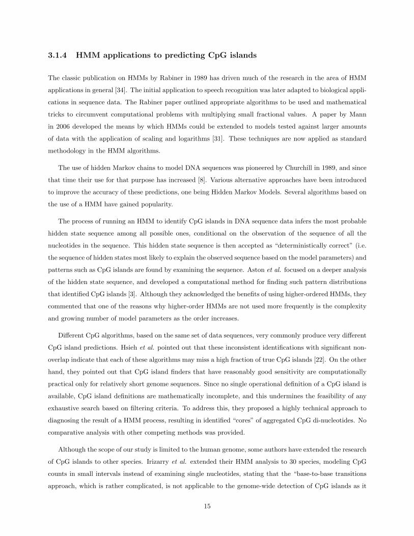
3.3 This diagram pictures the recursive nature of the Forward variable where each value at timepoint t+1 is based on the sum of values at time point t. . . . . . . . . . . . . . . . . . . . . 19

3.4 Viterbi decoding step from one observation to the next. All probabilities are as given by thetrained Hidden Markov Model. The hidden state generated by the step is determined by thestate with the maximum weight. . . . . . . . . . . . . . . . . . . . . . . . . . . . . . . . . . . 22

4.1 Typical output display produced by the CpGID 2.0 program. The two tracks at the bottomof the screen identify the start of a predicted CpG island within the data sequence by a greenvertical line and the end with a vertical red line. The black vertical bars of the top trackindicate the number of C and G nucleotides observed within each sliding window length versusthe expected number, where the maximum value detected is represented by a vertical barwith a height scaled to the track itself. The bottom track contains black vertical bars thatrepresent the ratio of island states to hidden states within each sliding window length, wherethe maximum calculated ratio is scaled to the height of the track. . . . . . . . . . . . . . . . 27

vi

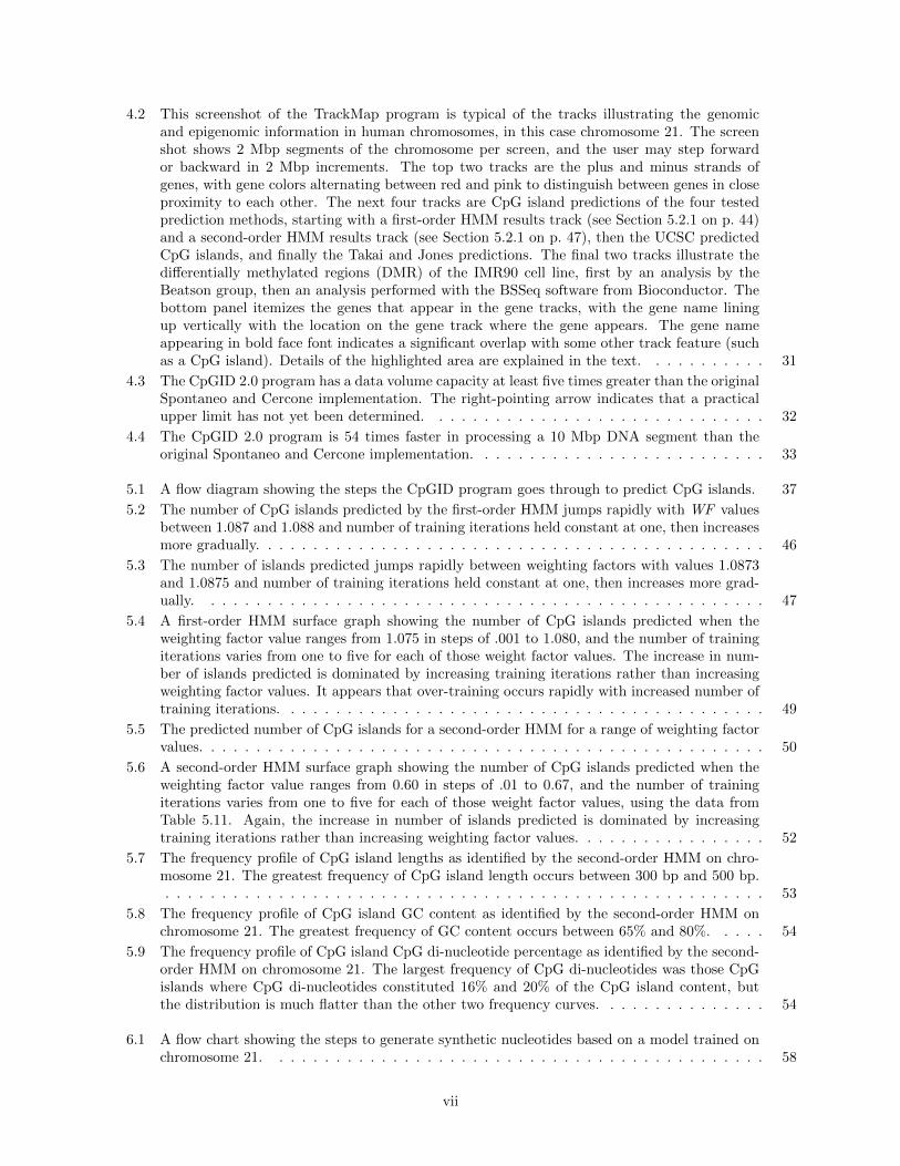
4.2 This screenshot of the TrackMap program is typical of the tracks illustrating the genomicand epigenomic information in human chromosomes, in this case chromosome 21. The screenshot shows 2 Mbp segments of the chromosome per screen, and the user may step forwardor backward in 2 Mbp increments. The top two tracks are the plus and minus strands ofgenes, with gene colors alternating between red and pink to distinguish between genes in closeproximity to each other. The next four tracks are CpG island predictions of the four testedprediction methods, starting with a first-order HMM results track (see Section 5.2.1 on p. 44)and a second-order HMM results track (see Section 5.2.1 on p. 47), then the UCSC predictedCpG islands, and finally the Takai and Jones predictions. The final two tracks illustrate thedifferentially methylated regions (DMR) of the IMR90 cell line, first by an analysis by theBeatson group, then an analysis performed with the BSSeq software from Bioconductor. Thebottom panel itemizes the genes that appear in the gene tracks, with the gene name liningup vertically with the location on the gene track where the gene appears. The gene nameappearing in bold face font indicates a significant overlap with some other track feature (suchas a CpG island). Details of the highlighted area are explained in the text. . . . . . . . . . . 31

4.3 The CpGID 2.0 program has a data volume capacity at least five times greater than the originalSpontaneo and Cercone implementation. The right-pointing arrow indicates that a practicalupper limit has not yet been determined. . . . . . . . . . . . . . . . . . . . . . . . . . . . . . 32

4.4 The CpGID 2.0 program is 54 times faster in processing a 10 Mbp DNA segment than theoriginal Spontaneo and Cercone implementation. . . . . . . . . . . . . . . . . . . . . . . . . . 33

5.1 A flow diagram showing the steps the CpGID program goes through to predict CpG islands. 37

5.2 The number of CpG islands predicted by the first-order HMM jumps rapidly with WF valuesbetween 1.087 and 1.088 and number of training iterations held constant at one, then increasesmore gradually. . . . . . . . . . . . . . . . . . . . . . . . . . . . . . . . . . . . . . . . . . . . . 46

5.3 The number of islands predicted jumps rapidly between weighting factors with values 1.0873and 1.0875 and number of training iterations held constant at one, then increases more grad-ually. . . . . . . . . . . . . . . . . . . . . . . . . . . . . . . . . . . . . . . . . . . . . . . . . . 47

5.4 A first-order HMM surface graph showing the number of CpG islands predicted when theweighting factor value ranges from 1.075 in steps of .001 to 1.080, and the number of trainingiterations varies from one to five for each of those weight factor values. The increase in num-ber of islands predicted is dominated by increasing training iterations rather than increasingweighting factor values. It appears that over-training occurs rapidly with increased number oftraining iterations. . . . . . . . . . . . . . . . . . . . . . . . . . . . . . . . . . . . . . . . . . . 49

5.5 The predicted number of CpG islands for a second-order HMM for a range of weighting factorvalues. . . . . . . . . . . . . . . . . . . . . . . . . . . . . . . . . . . . . . . . . . . . . . . . . . 50

5.6 A second-order HMM surface graph showing the number of CpG islands predicted when theweighting factor value ranges from 0.60 in steps of .01 to 0.67, and the number of trainingiterations varies from one to five for each of those weight factor values, using the data fromTable 5.11. Again, the increase in number of islands predicted is dominated by increasingtraining iterations rather than increasing weighting factor values. . . . . . . . . . . . . . . . . 52

5.7 The frequency profile of CpG island lengths as identified by the second-order HMM on chro-mosome 21. The greatest frequency of CpG island length occurs between 300 bp and 500 bp.. . . . . . . . . . . . . . . . . . . . . . . . . . . . . . . . . . . . . . . . . . . . . . . . . . . . . 53

5.8 The frequency profile of CpG island GC content as identified by the second-order HMM onchromosome 21. The greatest frequency of GC content occurs between 65% and 80%. . . . . 54

5.9 The frequency profile of CpG island CpG di-nucleotide percentage as identified by the second-order HMM on chromosome 21. The largest frequency of CpG di-nucleotides was those CpGislands where CpG di-nucleotides constituted 16% and 20% of the CpG island content, butthe distribution is much flatter than the other two frequency curves. . . . . . . . . . . . . . . 54

6.1 A flow chart showing the steps to generate synthetic nucleotides based on a model trained onchromosome 21. . . . . . . . . . . . . . . . . . . . . . . . . . . . . . . . . . . . . . . . . . . . 58

vii

6.2 Surface graph illustrating the second-order HMM CpG island predictions of the generatedsynthetic data with “planted” CpG islands. . . . . . . . . . . . . . . . . . . . . . . . . . . . . 63

7.1 The frequency profile of CpG island lengths as identified by the second-order HMM on chro-mosome 22. . . . . . . . . . . . . . . . . . . . . . . . . . . . . . . . . . . . . . . . . . . . . . 66

8.1 This simple diagram illustrates the “hidden state switch” phenomenon using an extreme ex-ample of comparison between two sequences with the same hidden state composition, butdifferent outcome due to the fact that case 1 has only one hidden state switch and case 2 has10. With a requirement for seven, or even six, hidden states in the sliding window of size 10in order to qualify as a CpG island, case 1 predicts one CpG island, and case 2 predicts none. 74

A.1 Screen shot of setup parameters for CpG Island Detection program. . . . . . . . . . . . . . . 84A.2 Screen shot of output for CpG Island Detection program. . . . . . . . . . . . . . . . . . . . . 85A.3 Screen shot of analysis of CpG islands for CpG Island Detection program. . . . . . . . . . . . 86

viii

List of Abbreviations

A Adenine nucleotideB Background hidden statebp base pairsbwd BackwardC Cytosine nucleotideCGI CpG islandsCpG Di-nucleotide consisting of cytosine followed by guanineCpGID CpG Island DetectionC# C# programming languageDMR Differentially methylated regionDNA Deoxyribonucleic acidFDR False Discovery RateFN False NegativeFP False Positivefwd ForwardG Guanine nucleotideGHz GigahertzGb Gigabytehg18 Human genome version 18hg19 Human genome version 19HMM Hidden Markov ModelI Island hidden stateMbp mega (1000) base pairsmiRNA microRNAN “Unknown” nucleotideNCBI National Center for Biotechnology InformationObs/Exp Observed/ExpectedPPV Positive predictive valuerRNA Ribosomal RNAsnRNA Small nuclear RNAsnoRNA Small nucleolar RNAT Thymine nucleotideTP True PositiveTPCF Two-Point Correlation FunctionTSS Transcription start siteUCSC University of California Santa CruzVB.Net Visual Basic.Net programming languageWF Weighting Factor

ix

Chapter 1

Introduction

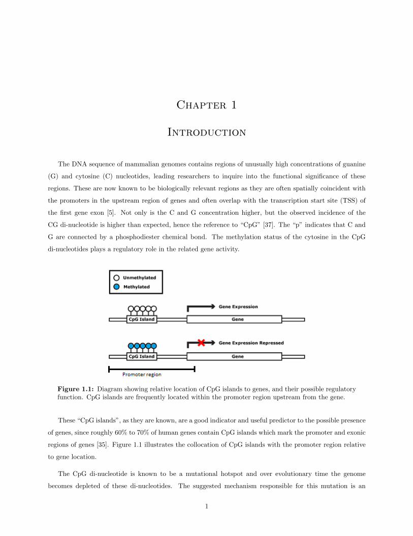
The DNA sequence of mammalian genomes contains regions of unusually high concentrations of guanine

(G) and cytosine (C) nucleotides, leading researchers to inquire into the functional significance of these

regions. These are now known to be biologically relevant regions as they are often spatially coincident with

the promoters in the upstream region of genes and often overlap with the transcription start site (TSS) of

the first gene exon [5]. Not only is the C and G concentration higher, but the observed incidence of the

CG di-nucleotide is higher than expected, hence the reference to “CpG” [37]. The “p” indicates that C and

G are connected by a phosphodiester chemical bond. The methylation status of the cytosine in the CpG

di-nucleotides plays a regulatory role in the related gene activity.

Figure 1.1: Diagram showing relative location of CpG islands to genes, and their possible regulatoryfunction. CpG islands are frequently located within the promoter region upstream from the gene.

These “CpG islands”, as they are known, are a good indicator and useful predictor to the possible presence

of genes, since roughly 60% to 70% of human genes contain CpG islands which mark the promoter and exonic

regions of genes [35]. Figure 1.1 illustrates the collocation of CpG islands with the promoter region relative

to gene location.

The CpG di-nucleotide is known to be a mutational hotspot and over evolutionary time the genome

becomes depleted of these di-nucleotides. The suggested mechanism responsible for this mutation is an

1

increased vulnerability of methylated cytosines in a CpG to spontaneously deaminate to thymine [38]. Thus

the average concentration of C and G nucleotides in the human genome is only about 41% (versus the expected

50%) [2], but because of the functional constraints in CpG islands, the concentration of these nucleotides in

the promoter region typically exceeds 55%.

This analysis can be carried one step further. Assuming that the number of C and G nucleotides making

up the 41% of the human genome are roughly equal, the statistical expectation that any pair of nucleotides

will consist of a cytosine followed by a guanine (i.e. a CpG di-nucleotide) is about 21% x 21%, or 4.41%.

The actual measured frequency of CpGs in the human genome is only 1%, leading to an observed/expected

ratio of 0.23. When this ratio for a given limited region of DNA exceeds 0.65 and the C and G concentration

exceeds 55%, this is a key indicator to the presence of a CpG island.

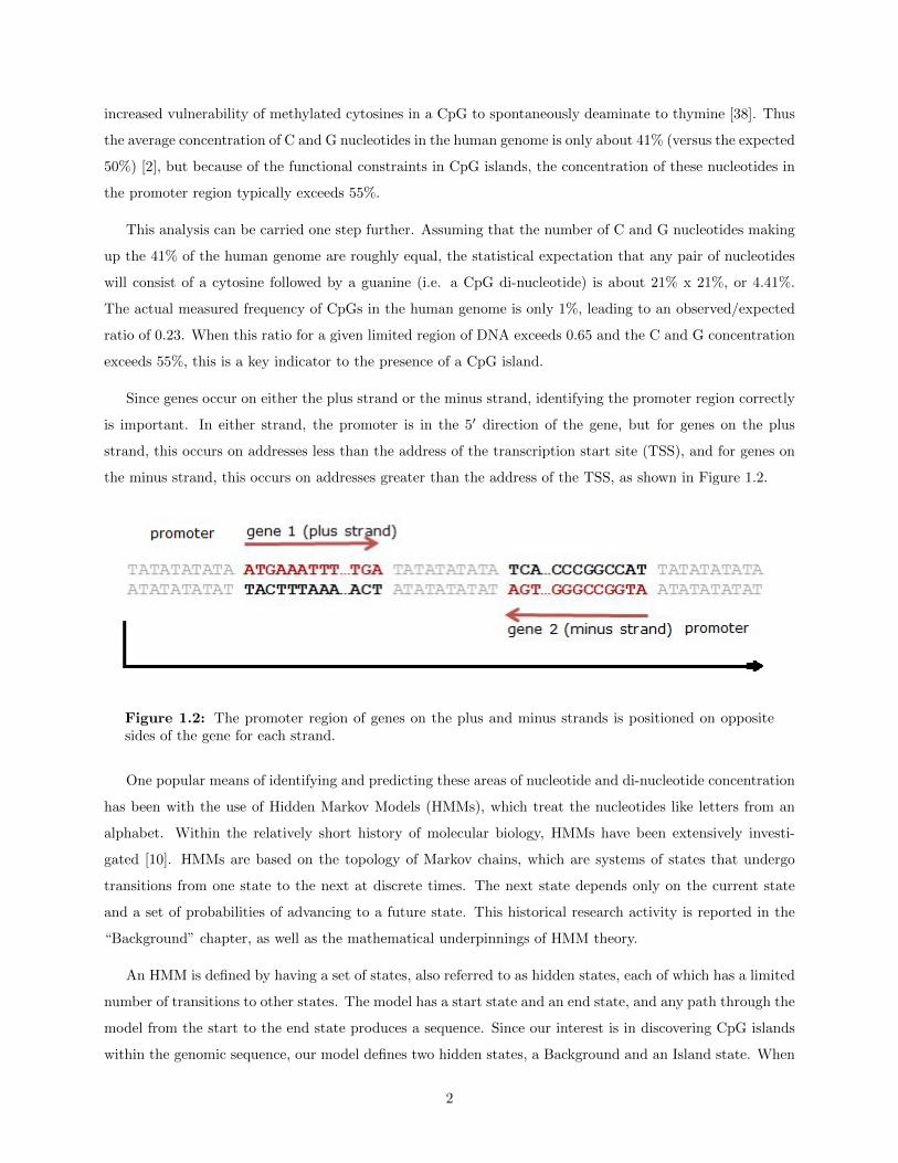
Since genes occur on either the plus strand or the minus strand, identifying the promoter region correctly

is important. In either strand, the promoter is in the 5′ direction of the gene, but for genes on the plus

strand, this occurs on addresses less than the address of the transcription start site (TSS), and for genes on

the minus strand, this occurs on addresses greater than the address of the TSS, as shown in Figure 1.2.

Figure 1.2: The promoter region of genes on the plus and minus strands is positioned on oppositesides of the gene for each strand.

One popular means of identifying and predicting these areas of nucleotide and di-nucleotide concentration

has been with the use of Hidden Markov Models (HMMs), which treat the nucleotides like letters from an

alphabet. Within the relatively short history of molecular biology, HMMs have been extensively investi-

gated [10]. HMMs are based on the topology of Markov chains, which are systems of states that undergo

transitions from one state to the next at discrete times. The next state depends only on the current state

and a set of probabilities of advancing to a future state. This historical research activity is reported in the

“Background” chapter, as well as the mathematical underpinnings of HMM theory.

An HMM is defined by having a set of states, also referred to as hidden states, each of which has a limited

number of transitions to other states. The model has a start state and an end state, and any path through the

model from the start to the end state produces a sequence. Since our interest is in discovering CpG islands

within the genomic sequence, our model defines two hidden states, a Background and an Island state. When

2

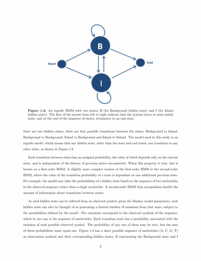
Figure 1.3: An ergodic HMM with two states, B (for Background hidden state) and I (for Islandhidden state). The flow of the arrows from left to right indicate that the system starts at some initialstate, and at the end of the sequence of states, terminates in an end state.

there are two hidden states, there are four possible transitions between the states, Background to Island,

Background to Background, Island to Background and Island to Iisland. The model used in this study is an

ergodic model, which means that any hidden state, other than the start and end states, can transition to any

other state, as shown in Figure 1.3.

Each transition between states has an assigned probability, the value of which depends only on the current

state, and is independent of the history of previous states encountered. When this property is true, this is

known as a first-order HMM. A slightly more complex version of the first-order HMM is the second-order

HMM, where the value of the transition probability of a state is dependent on one additional previous state.

For example, the model may infer the probabilities of a hidden state based on the sequence of two nucleotides

in the observed sequence rather than a single nucleotide. A second-order HMM thus encapsulates double the

amount of information about transitions between states.

As each hidden state can be inferred from an observed symbol, given the Markov model parameters, each

hidden state can also be thought of as generating a limited number of emissions from that state, subject to

the probabilities defined by the model. The emissions correspond to the observed symbols of the sequence,

which in our case is the sequence of nucleotides. Each transition state has a probability associated with the

emission of each possible observed symbol. The probability of any one of these may be zero, but the sum

of these probabilities must equal one. Figure 1.4 has a short possible sequence of nucleotides (A, C, G, T)

as observation symbols and their corresponding hidden states, B representing the Background state and I

3

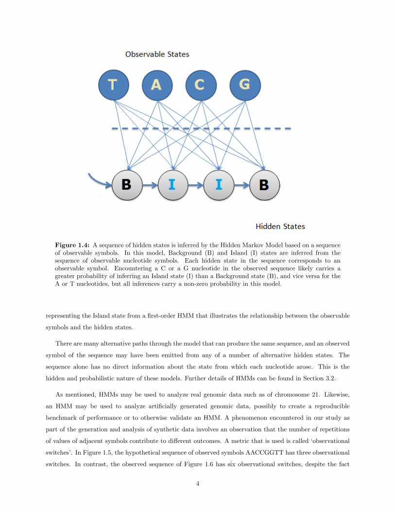
Figure 1.4: A sequence of hidden states is inferred by the Hidden Markov Model based on a sequenceof observable symbols. In this model, Background (B) and Island (I) states are inferred from thesequence of observable nucleotide symbols. Each hidden state in the sequence corresponds to anobservable symbol. Encountering a C or a G nucleotide in the observed sequence likely carries agreater probability of inferring an Island state (I) than a Background state (B), and vice versa for theA or T nucleotides, but all inferences carry a non-zero probability in this model.

representing the Island state from a first-order HMM that illustrates the relationship between the observable

symbols and the hidden states.

There are many alternative paths through the model that can produce the same sequence, and an observed

symbol of the sequence may have been emitted from any of a number of alternative hidden states. The

sequence alone has no direct information about the state from which each nucleotide arose. This is the

hidden and probabilistic nature of these models. Further details of HMMs can be found in Section 3.2.

As mentioned, HMMs may be used to analyze real genomic data such as of chromosome 21. Likewise,

an HMM may be used to analyze artificially generated genomic data, possibly to create a reproducible

benchmark of performance or to otherwise validate an HMM. A phenomenon encountered in our study as

part of the generation and analysis of synthetic data involves an observation that the number of repetitions

of values of adjacent symbols contribute to different outcomes. A metric that is used is called ‘observational

switches’. In Figure 1.5, the hypothetical sequence of observed symbols AACCGGTT has three observational

switches. In contrast, the observed sequence of Figure 1.6 has six observational switches, despite the fact

4

that compositionally the sequences have the same count of each symbol.

Figure 1.5: A hypothetical sequence of observational symbols and their corresponding possible hiddenstates. This sequence has three observational switches and two hidden state switches, B-> and I->B.

Figure 1.6: A hypothetical sequence of observational symbols and their corresponding possible hiddenstates. Even though this sequence has the same compositional elements as Figure 1.5, this sequencehas six observational switches and three hidden state switches.

Correspondingly consider the hypothetical hidden state sequences associated with each sequence of obser-

vational symbols. Each time the hidden state changes from one state to a different state is called a ‘hidden

state switch’. In spite of the fact that both figures have the same count of hidden states, four Background

(B) states and four Island (I) states, the count of ‘hidden state switches’ in Figure 1.6 (3) is one greater than

the count in Figure 1.5 (2). This concept is relevant to the discussion in Section 8.3.

A software module published by Spontaneo and Cercone provides much of the motivation behind the types

of questions asked in our study [42]. The software is referred to as the CpG Island Detection 1.0 program,

or CpGID 1.0. After investigating the capabilities of this software, various limitations and shortcomings

were identified that directly affected the accuracy and quality of the outcomes of the program. The memory

limitations and inefficiency of the software made it impossible to apply the HMM analysis to any significant

sequence length, such as a complete eukaryotic chromosome. Once these limitations were overcome, it was

discovered that aggregating the results of applying the same model parameters to consecutive segments of a

sequence was not equivalent to the results obtained when applying the HMM to all segments combined. For

example, the sum of predicted CpG islands of five consecutive segments of chromosome 21 was 235, but the

number of predicted CpG islands for the chromosome when tested as a whole was only 2. In other words, in

this case the sum of the parts was not equal to the whole.

The aims of this study are itemized in the “Objectives” chapter, but in summary they can be described as

addressing algorithmic deficiencies in the original computational implementation of the HMM, demonstrating

the anomalous behaviour of HMMs under certain conditions, and comparing the outcomes of various methods

5

of CpG island prediction such as the first-order HMM, the second-order HMM, the Takai and Jones method,

and the UCSC method. The Takai and Jones method uses a set of criteria (described below) based solely

on the sequence data and does not use HMM theory. One advantage that it offers over the UCSC method

is that it is available as a software component to run against the same data set as the HMM methods. In

the case of the UCSC method, only the mapped CpG islands are available for comparison. Further details

of each of these methods is provided in Chapter 5.

Although algorithms using an HMM can be shown to be superior to the Takai and Jones algorithm, our

study indicates that such a conclusion must be used with caution. The outcome depends largely on the initial

estimation for emission probabilities from one observation to the next to identify the ‘hidden’ CpG island

state. Our study illustrates this sensitivity to initial conditions.

As stated earlier, one of the biggest challenges facing effective analysis of DNA sequence data by HMMs

is the volume of data to be processed. The requirement to process an entire chromosome as a single unit has

implications both for memory storage of interim data structures, as well as for processing times. HMMs have

a reputation of being compute-intensive [30], a situation exacerbated by the need to apply them to a large

amount of data when used in realistic biological situations. This study addresses this issue by implementing

some computational and algorithmic short-cuts that result in a dramatic reduction in processing time by

several orders of magnitude. Judicious use of peripheral storage combined with streamlining of algorithmic

processes resulted in performance improvements enabling the kind of “what if” analysis that is frequently

required when doing HMM fine-tuning. When a whole series of tests can be run against a range of input

parameters, these tests are referred to as “blanket tests”.

This type of iterative testing becomes important under the conditions discovered where the outcomes

resulting from the HMM are highly dependent on the set of probability estimates initially set for the model.

One of the most significant findings of this study is that a small difference in the input parameters of the

HMM can result in a large difference in the predicted number of CpG islands. Finding where those large

differences occur in a range of input parameters leads to improved decisions about what the appropriate

input parameters are for a particular combination of HMM and data set. The blanket tests available in the

CpGID 2.0 program also provide a methodology for others to make the same determination for their HMM

and data.

The remainder of this document contains the following chapters: “Objectives”, “Background”, “CpGID

Program Improvements”, “Impact of initial parameter settings”, “Synthetic data generation”, “Comparison

with chromosome 22” and finally, “Discussion, Conclusions and Future Work”. The “Objectives” chapter

outlines the approach used for this project and itemizes the specific areas on which this project focused, as

well as some of the limitations of the project.

The “Background” chapter provides some of the nuances of HMM theory and the algorithms needed

6

to fully appreciate the findings of the later sections. Since the topic of HMMs, and CpG island prediction

in general, has been extensively studied, the “Background” chapter presents a historical overview of the

rich variety of ways in which this problem has been approached. Another subsection presents a theoretical

background of HMMs, explaining why they are more than just a solution looking for a problem. Several

of the algorithms used to implement HMMs are detailed. The backdrop of the details and limitations of

the original Spontaneo and Cercone HMM implementation are described to give a context within which this

project evolved.

Each of the next four chapters represent a separate, but related, facet of this study. Each of these

chapters contains a “Methodology” and “Results” section to provide a framework that describes each facet.

The “CpGID Program Improvements” chapter describes the technical requirements for the implementation

of the algorithms, describes vital programming improvements in the HMM algorithm implementation, and

quantifies the impact of algorithmic changes in the CpGID program in terms of processing and memory

performance improvement. The chapter on “Impact of initial parameter settings” presents the parameters

of the project — the data involved and how it was prepared. The approach used to relate predicted CpG

islands to gene promoter locations is described. This chapter also describes the methodology for how HMM

parameters are adjusted for both first-order and second-order HMMs to observe their effect on the outcome,

and reports the anomalous outcomes of first-order and second-order HMMs for certain initial parameter

estimates. The anomalous outcomes are a matter of interest for HMMs in general, not only in connection

with their application to CpG island prediction.

Two strategies for generating synthetic data are described and evaluated in the “Synthetic data genera-

tion” chapter. The “Comparison with chromosome 22” chapter highlights the dissimilar nature of chromosome

22 versus chromosome 21, and details the comparison of outcomes when the second-order HMM is applied

to chromosome 22.

The “Discussion, Conclusions and Future Work” chapter discusses the implications of the findings of our

thesis, explains the results obtained, recommends some best practices, and explores ways that the current

work could be extended.

7

Chapter 2

Objectives

The main intent of this thesis is to improve the ability to accurately predict the loci of CpG islands within

a DNA sequence using a Hidden Markov Model (HMM), as well as to offer programming improvements to an

HMM implementation that contribute to greater capacity and correctness. The HMM predicts and identifies

the location and size of CpG islands based strictly on observed characteristics of the nucleotides of the DNA

sequence.

A starting point for this work was the HMM implementation of Spontaneo and Cercone [42]. Preliminary

analysis indicated various shortcomings with the implementation. This thesis deconstructs the Spontaneo

and Cercone implementation, identifies issues and problems, analyzes the behaviour of HMMs in general,

and extends the CpGID 1.0 implementation to:

• identify errors and limitations in existing HMM packages (4.1.4);

• handle large amounts of data (e.g. complete eukaryotic chromosomes) (4.2.1);

• identify algorithmic changes to improve the HMM run-time performance to the extent that large

amounts of data can be processed in a reasonable amount of time (4.2.1);

• explore the impact of initial estimated parameters on HMM outcomes (Chapter 5);

• make recommendations on best practices when applying HMMs to the prediction of CpG islands (8.5);

• extend the first-order HMM to a second-order HMM to potentially improve prediction by taking ad-

vantage of the greater than expected frequency of occurrence of the CpG di-nucleotide in CpG islands,

using the fact that the second-order HMM can consider whether the previous pair of nucleotides was

a CG, rather than simply considering whether the previous single nucleotide was either a C or G as in

the case of the first-order HMM (5.1.3);

• compare CpG island predictions of human chromosome 21 with predictions of previously published

algorithms (5.2);

• compare the accuracy of CpG island predictions of human chromosome 21 with predictions of human

chromosome 22, and highlight any noticeably different characteristics between the two (Chapter 7);

8

• derive synthetic data from an HMM trained on real data and compare the composition and structure

of the two data sets (6.1.1);

• synthesize data containing pre-specified “planted” CpG islands to validate an HMM (6.1.1);

• explore the relationship between CpG islands, their methylation status and differentially methylated

regions (4.1.4).

The developed software is referred to as CpGID 2.0, or the CpG Island Detection 2.0 program. The

related visualization component is named the TrackMap program.

This thesis limits its focus primarily on the data of human chromosome 21 and secondarily on chromosome

22, and does not extend its analysis to the whole human genome or to other species. These and other

limitations are mentioned in the “Future Work” subsection as areas that could be addressed.

9

Chapter 3

Background

3.1 Historical

Epigenetics, a general area of study in which CpG islands play a large role, is an important regulatory

contributor to genomic expression, particularly through the effect of the methylation status in CpG islands.

The investigation of the relationship of CpG islands to methylation status, and subsequently to genomic

expression is an active area of research.

The significance of the biological function of CpG islands has been well documented, making their detec-

tion and identification an important bioinformatics goal. By 1987 the knowledge that CpG islands served as

gene markers was well established [5]. A canonical publication that established the link between CpG islands

and methylation, and the methylation mechanism of DNA methyltransferase proteins DNMT1, DNMT3A

and DNMT3B, was the paper by Bird in 2002 [4]. A recent overview of CpG islands by Illingworth and

Bird highlights the tissue-specific role of differential methylation of CpG islands, not only between different

tissues, but also between normal and malignant cells, leading to improper gene silencing [24].

A milestone paper by Yamada et al. in 2004 annotated many of the genes and their association with

CpG islands on human chromosome 21q [49], and reported on the methylation status of the CpG islands

for normal peripheral blood cells. Their analysis revealed that 103 of the 149 CpG islands examined were

non-methylated, and 31 were fully methylated. The remainder showed composite methylation. Lister et al.

describe various methods of deducing methylation status based on bisulfite technologies and how regions of

the human genome are characterized by methylation status [29].

Even though human chromosome 21 is the shortest of the autosomal chromosomes, it still consists of

over 48 million base pairs. Chromosome 21 is known to contain between 200 and 400 genes, depending on

the characterization of the genes. The larger count is dominated by known protein-coding genes and non-

functional pseudogenes, but also includes functional but non-protein coding miRNA, rRNA, snRNA, and

snoRNA genes. One early researcher suggested that there are 225 coding genes on this chromosome [14].

The Ensembl effort identified 240 putative protein-coding genes [13], but predicting and identifying the

10

remaining genes on this chromosome is an active area of genetic research.

3.1.1 Early attempts to define and identify CpG islands

The challenge to detect and predict CpG islands in the human genome has a long history, driven by the

importance of the biological association between CpG islands and the promoters of genes. As early as 1987

the unique motif of CpG islands was recognized and a simple algorithm to recognize them was formulated

by Gardiner-Garden and Frommer [15]. Their algorithm used a sliding window of size equal to a specified

minimum length for the definition of a CpG island, and applied the following criteria to determine whether

the region consisted of a CpG island. The three criteria parameters are:

1. Minimum G or C content of at least 50%.

2. Minimum observed CpG / expected CpG of at least 0.60.

3. Minimum length of at least 200 bp.

At any point where all three criteria were met, the length of the predicted island was extended from the

minimum length until either of the first two criteria were no longer met. Note that these thresholds are

arbitrary, indirect and subjective. Furthermore the first two criteria are not independent, suggesting a

possible source of bias.

The second criterion requires some explanation. As previously mentioned, the chemical nature of the

CpG di-nucleotide is such that it is subject to mutation and depletion over evolutionary time, resulting in

an observed/expected ratio of only 0.23. In the CpG island regions, however, the frequency is often observed

to be about three times the 0.23 ratio. Based on this observation, Gardiner-Garden and Frommer set their

observed/expected ratio threshold to 0.60.

The parameters chosen by Gardiner-Garden and Frommer for this algorithm were such that they resulted

in a large number of false positive identifications, where although CpG islands were predicted by the criteria,

the predictions were evidently not related to gene expression. This situation was corrected by Takai and

Jones in 2002 [44]. The revised parameters they introduced to predict the location of CpG islands in DNA

genomic sequences and their benchmark study of CpG islands on human chromosome 21 and 22 provided a

standard against which many subsequent researchers have measured their results. The criteria parameters

as revised by Takai and Jones are:

1. Minimum G or C content of at least 55%.

2. Minimum observed CpG / expected CpG of at least 0.65.

3. Minimum length of at least 500 bp.

11

The debate continues as to what the correct criteria are for identifying CpG islands in the human genome

as gene markers. For example, Wang et al. apply the Takai and Jones criteria and achieve a high level of

sensitivity in identifying CpG islands with annotated genes, but at low specificity [45]. In another effort,

Kim published another search algorithm that built on the Takai and Jones method by simply adding two

further criteria, one that specified the mean number of CpGs within the island [27]. The other specified the

gap between successively adjacent CpG islands, meant to exclude “mathematical CpG islands”. Nothing in

this method addresses the fundamental limitations of the filtering criteria approach.

3.1.2 Non-HMM algorithms for predicting CpG islands

Many alternative competing software approaches and algorithms have been published to predict the incidence

of CpG islands in a DNA sequence, suggesting various metrics and measurements to quantify the incidence

of CpG islands. The early approaches all relied on the largely subjective criteria of the thresholds of GC

content, CpG ratio and length. In an effort to establish an objective standard for defining CpG islands,

several researchers applied distance-based approaches that focused on CpG locations and concentrations as

the most natural sequence-based indicator of functional CpG islands.

Hackenberg et al. proposed a method called CpGcluster to predict statistically significant clusters of CpG

di-nucleotides based only on the distance between two consecutive CpG di-nucleotides [18]. Although the

CpGcluster method was efficient and had the advantage of starting and ending on a CpG di-nucleotide, as

well as including CpG islands smaller than the Takai and Jones sliding window size, Han et al. demonstrated

that based on various measurements, the Takai and Jones algorithm was more appropriate for identifying

promoter-associated CpG islands [20]. Hackenberg et al. responded by pointing out that with certain

parameters changes, CpGcluster was clearly superior to the Takai and Jones method [17].

In an algorithm called CpG Island Finder (CpGIF), Ye et al. extended the algorithm of CpGcluster by

focusing on high CpG density regions subject to a density cutoff threshold [50]. This “seed” region was then

extended by relaxing the default density. The algorithm suffers from low specificity, as the number of CpG

islands predicted for chromosome 21 was 3371, far in excess of the number of genes or the number of CpG

islands now assessed on the chromosome. There was no attempt made to correlate this prediction with gene

locations.

In another distance-based algorithm, Su et al. applied the theory of mutual information to the problem of

CpG island prediction [43]. Using the location of CpG di-nucleotides and the physical distance between two

neighboring CpGs as the two variables contributing to the mutual information, the algorithm was slightly

more accurate than prevailing algorithms such as CpGIF and CpGcluster. A major contribution of the analy-

sis, however, was the comparison of CpG island prediction with gene locations and with histone modifications

as important epigenetic regulatory elements. The overlap of predicted CpG islands and histone modification

12

Figure 3.1: The distribution of CpG islands in different genome regions, as reported by Su et al. [43].Note that chromsome 21 and chromosome Y have the lowest percentages located in the promoterregion.

tags suggested a role for CpG islands affecting open chromatin for active gene expression. The proximity of

CpG islands to promoter regions and genes was expressed as percentages, as shown in Figure 3.1. The low in-

cidence of CpG islands co-resident with promoter regions in chromosome 21 compared to other chromosomes

suggests that chromosome 21 is atypical in this statistic.

Singer et al. applied a 5-th order Markov model to DNA sequences to specifically predict coding CpG

islands, based on the assumption that CpG islands in coding regions are subject to different patterns of

codon usage and constraints than non-coding regions [40]. Their study revealed several coding CpG islands

in coding exons which were felt to be examples of functional epigenetic specialization within the gene.

Liu et al. employed higher-order and variable-order Markov chains to identify boundaries of CpG is-

lands [30]. They were critical of HMMs due to the fact that they can only be guaranteed to converge to

a local minimum, and cannot be trained in less than polynomial time. Our study suggests that this is not

necessarily true. Somewhat counter-intuitively, Liu et al. felt that their variable-order and higher-order

Markov chain were less complex than first-order chains, and produced higher accuracies, but their published

results on three DNA sequences do not bear that out.

Motivated by galaxy clustering in the universe, Koester et al. adapted and applied the two-point corre-

lation function (TPCF) used widely in astrophysics to characterize the organization of the universe to the

organization of CpG islands in the human genome [28]. Although they relied on the traditional Takai and

Jones method to identify the CpG islands, the TPCF method allowed them to quantitatively establish that

the distribution of CpG islands is non-random across each chromosome and varies significantly among chro-

13

mosomes. Just as galaxies have little structure on large scales in the universe, TPCF values indicated that

CpG islands have little or no structure at scales larger than a few Mbp. At smaller scales, however, there

was more evidence for “clustering” of CpG islands, pointing to a possible global organizational principle that

genes are positioned so as to exploit the chromatin packing machinery that regulates transcription.

Other machine-learning approaches such as neural networks and support vector machines have also been

applied to the predictive analysis of biological data. The efforts identified in this section illustrate that

there are many algorithms and approaches that can be, and have been, used for CpG island prediction, and

although some of them belong to a class of Markovian solutions, they are not necessarily Hidden Markov

Models.

3.1.3 Markov applications to other genetic problems

In 1999, Salzberg et al. used an Interpolated Markov approach to identify genes in the malaria parasite

Plasmodium falciparum [36]. Although not a true HMM, it treated the gene exons, introns and splice sites as

features in a Markov chain and shared the idea of training on a set of representative data. An Interpolated

Markov Model can be thought of as a combination of Markov chains of different orders, and considers the

frequencies of sequences of symbols of variable length in learning and building a probabilistic model from the

training data. Xie et al. applied a similar technique in 2004 to the problem of identifying co-expressed genes

in Saccharomyces cerevisiae [47], and Kazemian et al. applied a technique based on a Interpolated Markov

Model in their effort to identify enhancers in the Drosophila melanogaster genome [26]. This, along with the

previously mentioned Markovian solutions to sequence problems, points out that HMMs belong to a large

class of general approaches to solving identification and prediction problems.

HMMs have been applied to other genomic sequences such as histone modification sites. Xu et al. used

an HMM to infer the states of differential histone modification sites between mouse embryonic stem cells and

neural progenitor cells [48]. Their approach successfully identified histone differentially modified sites of the

H3K27me3 histone with high sensitivity, specificity, and reproducibility.

The popular HMMER software and web site is used for searching sequence databases for homologs of

protein sequences [12]. It implements methods using probabilistic models called profile hidden Markov models

(profile HMMs).

Although higher-order Markov chains have found biological application, the inherent difficulties with

higher-order HMMs such as computational feasibility have resulted in few publications relating high-order

HMMs to biological applications. One exception is a brief development of a high-order HMM by Ching et al.

that identifies a second-order HMM as superior to a first-order HMM, but fails to clearly demonstrate how

this was accomplished and at what computational cost [7].

14

3.1.4 HMM applications to predicting CpG islands

The classic publication on HMMs by Rabiner in 1989 has driven much of the research in the area of HMM

applications in general [34]. The initial application to speech recognition was later adapted to biological appli-

cations in sequence data. The Rabiner paper outlined appropriate algorithms to be used and mathematical

tricks to circumvent computational problems with multiplying small fractional values. A paper by Mann

in 2006 developed the means by which HMMs could be extended to models tested against larger amounts

of data with the application of scaling and logarithms [31]. These techniques are now applied as standard

methodology in the HMM algorithms.

The use of hidden Markov chains to model DNA sequences was pioneered by Churchill in 1989, and since

that time their use for that purpose has increased [8]. Various alternative approaches have been introduced

to improve the accuracy of these predictions, one being Hidden Markov Models. Several algorithms based on

the use of a HMM have gained popularity.

The process of running an HMM to identify CpG islands in DNA sequence data infers the most probable

hidden state sequence among all possible ones, conditional on the observation of the sequence of all the

nucleotides in the sequence. This hidden state sequence is then accepted as “deterministically correct” (i.e.

the sequence of hidden states most likely to explain the observed sequence based on the model parameters) and

patterns such as CpG islands are found by examining the sequence. Aston et al. focused on a deeper analysis

of the hidden state sequence, and developed a computational method for finding such pattern distributions

that identified CpG islands [3]. Although they acknowledged the benefits of using higher-ordered HMMs, they

commented that one of the reasons why higher-order HMMs are not used more frequently is the complexity

and growing number of model parameters as the order increases.

Different CpG algorithms, based on the same set of data sequences, very commonly produce very different

CpG island predictions. Hsieh et al. pointed out that these inconsistent identifications with significant non-

overlap indicate that each of these algorithms may miss a high fraction of true CpG islands [22]. On the other

hand, they pointed out that CpG island finders that have reasonably good sensitivity are computationally

practical only for relatively short genome sequences. Since no single operational definition of a CpG island is

available, CpG island definitions are mathematically incomplete, and this undermines the feasibility of any

exhaustive search based on filtering criteria. To address this, they proposed a highly technical approach to

diagnosing the result of a HMM process, resulting in identified “cores” of aggregated CpG di-nucleotides. No

comparative analysis with other competing methods was provided.

Although the scope of our study is limited to the human genome, some authors have extended the research

of CpG islands to other species. Irizarry et al. extended their HMM analysis to 30 species, modeling CpG

counts in small intervals instead of examining single nucleotides, stating that the “base-to-base transitions

approach, which is rather complicated, is not applicable to the genome-wide detection of CpG islands as it

15

requires CpG islands to be predetermined for a training step” [25]. However, nothing in the results suggests

that their approach is advantageous to a base-to-base transitions approach and the only factor that would

make the base-to-base approach more complicated is the increased volume of data to be handled.

3.2 Theoretical background of HMMs

The foundation of the single-layer Markov chain provides the basic building blocks for the ability of an HMM

to describe biological sequence data. The HMM provides additional information in quantitatively describing

observation sequences from the viewpoint of an underlying hidden layer. The higher complexity of the HMM

is justified by the greater range of possible probabilistic processes that can be used to generate, describe, and

solve problems in sequence analysis [34].

An HMM is defined as a system M = (Q, S, A, B, Π), consisting of

1. an alphabet Q (a set of observable unique symbols),

2. a set of hidden states S,

3. a matrix A = {akl} of transition probabilities {akl} for k,l ∈ S ; i.e. the probability of going from any

one state to any other state for all states in S,

4. a matrix B = {ek(q)} of emission probabilities {ek(q)} for every k ∈ S and q ∈ Q ; i.e. the probability

of emitting each symbol in Q from each hidden state in S,

5. a vector Π = {πi} of initial state probabilities {πi} for every i ∈ S ; i.e. the probability of starting in

state i for each state in S.

The discrete point t is an element of the set of all time points ending at T, denoted as t ∈ {1, 2, . . . ,T}.

The random variable O defines the sequence of observable symbols o from the alphabet Q of length T. Each

observable symbol corresponds to an element in a hidden state sequence at a discrete point t denoted as xt

and its state at point t is denoted st, where st ∈ S. For a model with two hidden states where s can take

on the values Background and Island, S = {Background, Island}. For a model that uses an alphabet of

nucleotide symbols, Q = {A, C, G, T}.

Figure 3.2 shows a short sequence of observed elements (ot drawn from the alphabet Q) from an HMM

and their corresponding hidden state elements (xt drawn from the set of hidden states S ).

Each hidden state in the sequence can be inferred from a symbol from the alphabet Q, or equivalently,

each symbol in the alphabet Q is said to be emitted from the hidden state, based on the probabilities of the

HMM, known collectively as the model parameters.

16

Figure 3.2: A short HMM sequence of observable symbols ot drawn from Q. The random variable Xdefines the sequence of hidden states xt drawn from the set of hidden states S. Transitions from onestate to another and one symbol to another occur between discrete points t and t+ 1.

An important property of the HMM is that of a transition probability. A system evolves with probabilistic

Markov dynamics if the probability of being in the future state st+1 depends only on the present state of st,

and not on the past states; i.e. P(st+1 | st,st−1,. . . ,s1) = P(st+1 | st) and st represents the actual state of the

element in the hidden state sequence at point t. As t increases from 1 to T along the chain, the states of the

subsequent elements in the chain are determined from states of the elements immediately preceding them

through a state transition probability. The transition probabilities are arranged into a transition matrix,

defined as A, which defines the possible transitions from any state to all other states, giving an N xN matrix

since X can attain any one of the N states. Table 3.1 gives an example of a simple transition probability

matrix for a model consisting of a Background hidden state and an Island hidden state.

Hidden State Background Island

Background: 0.8 0.2

Island: 0.6 0.4

Table 3.1: An example of a simple transition probability matrix. Each element indicates the proba-bility of transitioning from a row state to a column state.

Associated with each of the elements from the hidden state space S is a set of emission probabilities that

establish the probabilities of emitting an observation symbol q from Q. These probabilities can be arranged

into an emission probability matrix defined as B, which defines the probability of emitting each observation

symbol from the given hidden state. Table 3.2 gives an example of an emission probability matrix for a model

with the hidden states described in Table 3.1 and the emitted symbols A, C, G, and T.

Hidden State A C G T

Background: 0.3 0.2 0.2 0.3

Island: 0.2 0.3 0.3 0.2

Table 3.2: An example of a simple emission probability matrix. Each element indicates the probabilityof emitting a column symbol from a row state.

An HMM needs to start in a certain state, and the initial state probabilities, defined as Π, define the

17

probability of starting in any one of the hidden states. Table 3.3 gives an example of an initial state probability

matrix for a model with the hidden states described in Table 3.1

Hidden State Probability

Background: 0.6

Island: 0.4

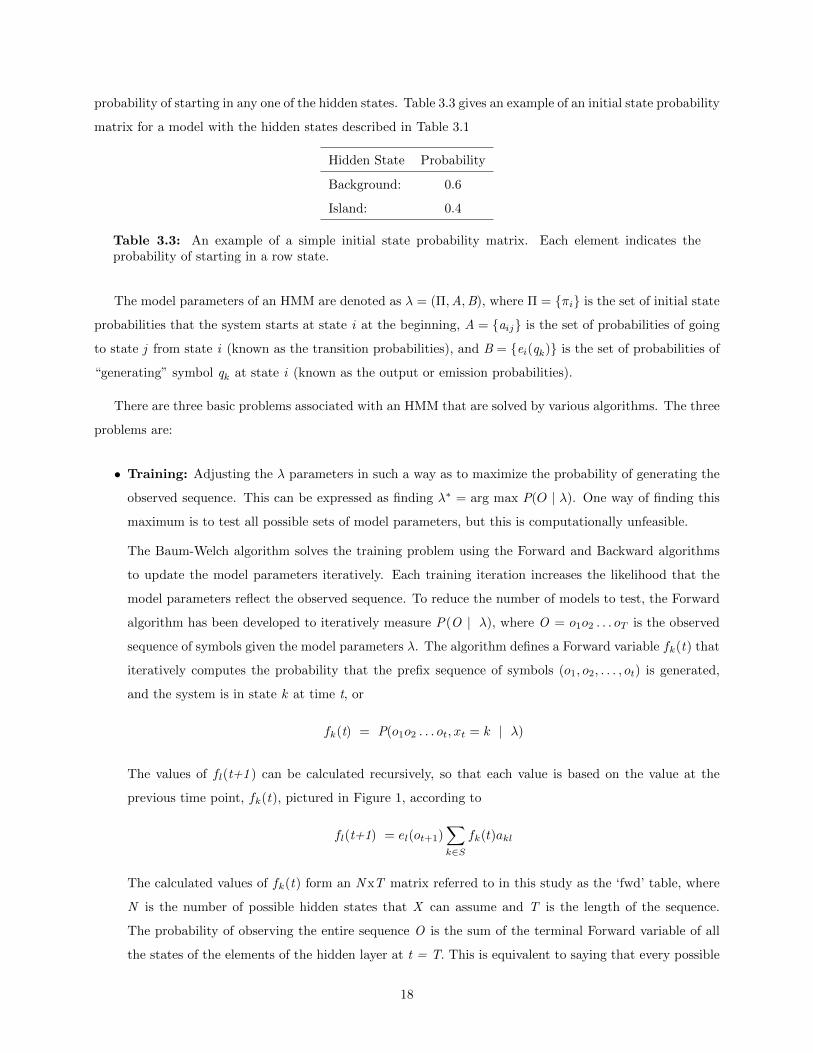
Table 3.3: An example of a simple initial state probability matrix. Each element indicates theprobability of starting in a row state.

The model parameters of an HMM are denoted as λ = (Π,A,B), where Π = {πi} is the set of initial state

probabilities that the system starts at state i at the beginning, A = {aij} is the set of probabilities of going

to state j from state i (known as the transition probabilities), and B = {ei(qk)} is the set of probabilities of

“generating” symbol qk at state i (known as the output or emission probabilities).

There are three basic problems associated with an HMM that are solved by various algorithms. The three

problems are:

• Training: Adjusting the λ parameters in such a way as to maximize the probability of generating the

observed sequence. This can be expressed as finding λ∗ = arg max P(O | λ). One way of finding this

maximum is to test all possible sets of model parameters, but this is computationally unfeasible.

The Baum-Welch algorithm solves the training problem using the Forward and Backward algorithms

to update the model parameters iteratively. Each training iteration increases the likelihood that the

model parameters reflect the observed sequence. To reduce the number of models to test, the Forward

algorithm has been developed to iteratively measure P(O | λ), where O = o1o2 . . . oT is the observed

sequence of symbols given the model parameters λ. The algorithm defines a Forward variable fk(t) that

iteratively computes the probability that the prefix sequence of symbols (o1, o2, . . . , ot) is generated,

and the system is in state k at time t, or

fk(t) = P(o1o2 . . . ot, xt = k | λ)

The values of fl(t+1 ) can be calculated recursively, so that each value is based on the value at the

previous time point, fk(t), pictured in Figure 1, according to

fl(t+1) = el(ot+1)∑k∈S

fk(t)akl

The calculated values of fk(t) form an N xT matrix referred to in this study as the ‘fwd’ table, where

N is the number of possible hidden states that X can assume and T is the length of the sequence.

The probability of observing the entire sequence O is the sum of the terminal Forward variable of all

the states of the elements of the hidden layer at t = T. This is equivalent to saying that every possible

18

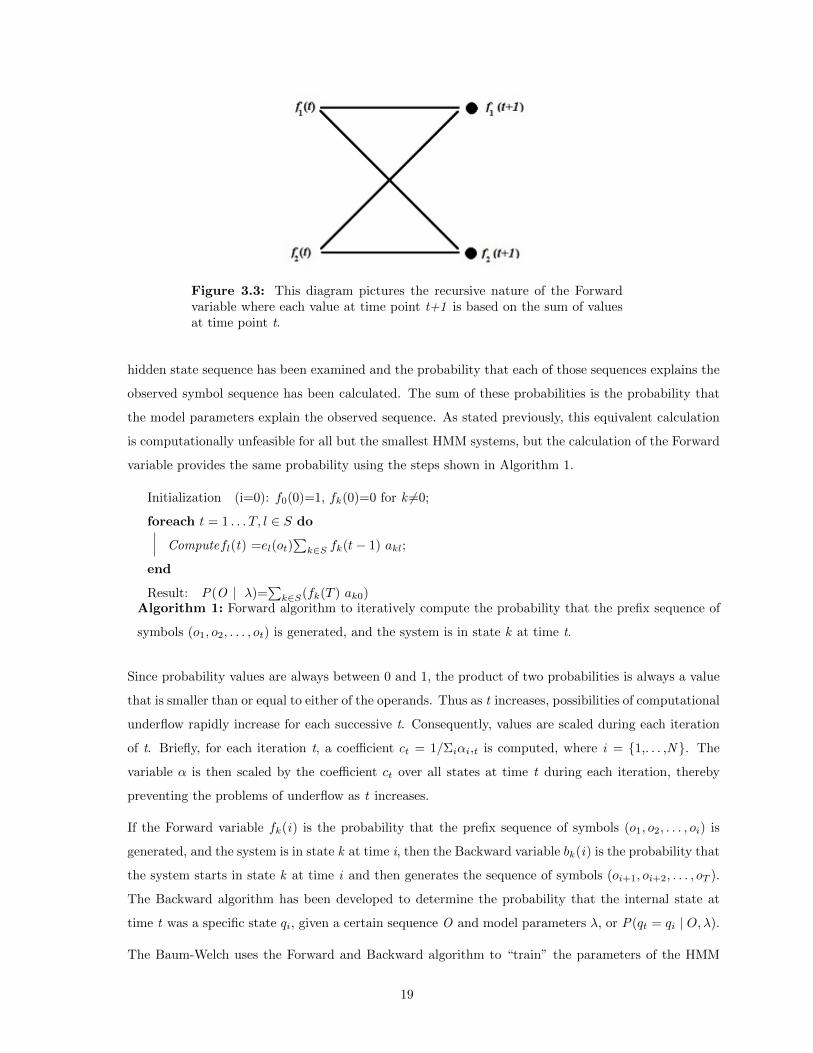
Figure 3.3: This diagram pictures the recursive nature of the Forwardvariable where each value at time point t+1 is based on the sum of valuesat time point t.

hidden state sequence has been examined and the probability that each of those sequences explains the

observed symbol sequence has been calculated. The sum of these probabilities is the probability that

the model parameters explain the observed sequence. As stated previously, this equivalent calculation

is computationally unfeasible for all but the smallest HMM systems, but the calculation of the Forward

variable provides the same probability using the steps shown in Algorithm 1.

Initialization (i=0): f0(0)=1, fk(0)=0 for k 6=0;

foreach t = 1 . . . T, l ∈ S do

Computefl(t) =el(ot)∑

k∈S fk(t− 1) akl;

end

Result: P(O | λ)=∑

k∈S(fk(T ) ak0)Algorithm 1: Forward algorithm to iteratively compute the probability that the prefix sequence of

symbols (o1, o2, . . . , ot) is generated, and the system is in state k at time t.

Since probability values are always between 0 and 1, the product of two probabilities is always a value

that is smaller than or equal to either of the operands. Thus as t increases, possibilities of computational

underflow rapidly increase for each successive t. Consequently, values are scaled during each iteration

of t. Briefly, for each iteration t, a coefficient ct = 1/Σiαi,t is computed, where i = {1,. . . ,N }. The

variable α is then scaled by the coefficient ct over all states at time t during each iteration, thereby

preventing the problems of underflow as t increases.

If the Forward variable fk(i) is the probability that the prefix sequence of symbols (o1, o2, . . . , oi) is

generated, and the system is in state k at time i, then the Backward variable bk(i) is the probability that

the system starts in state k at time i and then generates the sequence of symbols (oi+1, oi+2, . . . , oT ).

The Backward algorithm has been developed to determine the probability that the internal state at

time t was a specific state qi, given a certain sequence O and model parameters λ, or P(qt = qi | O, λ).

The Baum-Welch uses the Forward and Backward algorithm to “train” the parameters of the HMM

19

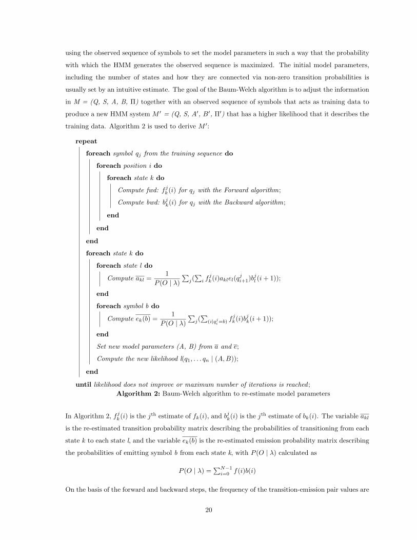
using the observed sequence of symbols to set the model parameters in such a way that the probability

with which the HMM generates the observed sequence is maximized. The initial model parameters,

including the number of states and how they are connected via non-zero transition probabilities is

usually set by an intuitive estimate. The goal of the Baum-Welch algorithm is to adjust the information

in M = (Q, S, A, B, Π) together with an observed sequence of symbols that acts as training data to

produce a new HMM system M ′ = (Q, S, A′, B′, Π′) that has a higher likelihood that it describes the

training data. Algorithm 2 is used to derive M ′:

repeat

foreach symbol qj from the training sequence do

foreach position i do

foreach state k do

Compute fwd: f jk(i) for qj with the Forward algorithm;

Compute bwd: bjk(i) for qj with the Backward algorithm;

end

end

end

foreach state k do

foreach state l do

Compute akl =1

P (O | λ)

∑j(∑

i fjk(i)aklel(q

ji+1)bjl (i+ 1));

end

foreach symbol b do

Compute ek(b) =1

P (O | λ)

∑j(∑

(i|qji=b) fjk(i)bjk(i+ 1));

end

Set new model parameters (A, B) from a and e;

Compute the new likelihood l(q1, . . . qn | (A,B));

end

until likelihood does not improve or maximum number of iterations is reached ;

Algorithm 2: Baum-Welch algorithm to re-estimate model parameters

In Algorithm 2, f jk(i) is the jth estimate of fk(i), and bjk(i) is the jth estimate of bk(i). The variable akl

is the re-estimated transition probability matrix describing the probabilities of transitioning from each

state k to each state l, and the variable ek(b) is the re-estimated emission probability matrix describing

the probabilities of emitting symbol b from each state k, with P (O | λ) calculated as

P (O | λ) =∑N−1

i=0f(i)b(i)

On the basis of the forward and backward steps, the frequency of the transition-emission pair values are

20

determined and divided by the probability of the entire string. Essentially this calculates the expected

count of each particular transition-emission pair. Each time a particular transition is found, the value

of the quotient of the transition count divided by the probability of the entire string increases, and this

value can then be made the new value of the transition probability. The likelihood calculated by the

Baum-Welch algorithm is guaranteed to converge to a local maximum value but not necessarily to a

global maximum value.

• Evaluation: Evaluating P(O | λ), the probability that an observed sequence of symbols O was pro-

duced by a particular HMM with model parameters λ.

This problem can also be viewed as evaluating how well a given model matches a given observation

sequence. In a case where there are competing models, the solution allows the model that best matches

the observation to be chosen. The solution is provided by the likelihoods calculated by the Forward

algorithm. The highest likelihood calculated identifies the model that best matches the observed se-

quence.

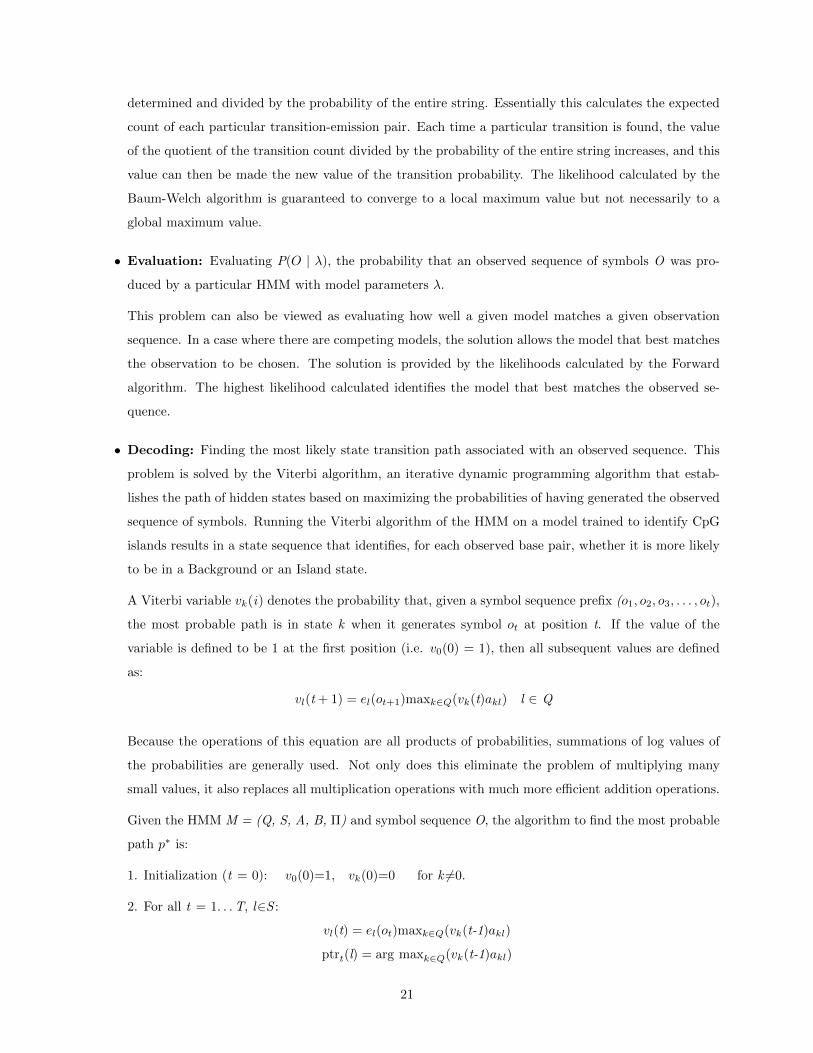
• Decoding: Finding the most likely state transition path associated with an observed sequence. This

problem is solved by the Viterbi algorithm, an iterative dynamic programming algorithm that estab-

lishes the path of hidden states based on maximizing the probabilities of having generated the observed

sequence of symbols. Running the Viterbi algorithm of the HMM on a model trained to identify CpG

islands results in a state sequence that identifies, for each observed base pair, whether it is more likely

to be in a Background or an Island state.

A Viterbi variable vk(i) denotes the probability that, given a symbol sequence prefix (o1, o2, o3, . . . , ot),

the most probable path is in state k when it generates symbol ot at position t. If the value of the

variable is defined to be 1 at the first position (i.e. v0(0) = 1), then all subsequent values are defined

as:

vl(t + 1) = el(ot+1)maxk∈Q(vk(t)akl) l ∈ Q

Because the operations of this equation are all products of probabilities, summations of log values of

the probabilities are generally used. Not only does this eliminate the problem of multiplying many

small values, it also replaces all multiplication operations with much more efficient addition operations.

Given the HMM M = (Q, S, A, B, Π) and symbol sequence O, the algorithm to find the most probable

path p∗ is:

1. Initialization (t = 0): v0(0)=1, vk(0)=0 for k 6=0.

2. For all t = 1. . . T, l∈S :

vl(t) = el(ot)maxk∈Q(vk(t-1)akl)

ptrt(l) = arg maxk∈Q(vk(t-1)akl)

21

The ptrt(l) is a table that keeps track of which state it was that gave the previous maximum weight.

This information is used in the Traceback step below to reconstruct the sequence of hidden states.

3. Termination (vk(T ) is the Viterbi variable at the final point in the observation sequence for state

k):

P (o,p∗) = maxk∈Q(vk(T)ak0)

p∗L = arg maxk∈Q(vk(T)ak0)

4. Traceback: For all t = T - 1. . . 1: p∗t−1 = ptrt(p∗t )

Figure 3.4: Viterbi decoding step from one observation to the next. All probabilities are as given bythe trained Hidden Markov Model. The hidden state generated by the step is determined by the statewith the maximum weight.

Figure 3.4 illustrates the general form of a single step of the Viterbi algorithm from one observation to

the next for the HMM model consisting of the two hidden states, Background (B) and Island (I). The

maximum weight, or probability of arriving at a Background state or Island state based on the previous

observation, is retained for each position of the symbol sequence. After this general form terminates,

the traceback step goes in the opposite direction and uses the ptrt(l) information to reconstruct the

entire sequence of hidden states.

22

3.3 Details of the Spontaneo and Cercone HMM implementation

Several researchers claim their HMM algorithms have superior CpG island predictive ability. In 2011, Spon-

taneo and Cercone published a paper that introduced their software for CpG island prediction using an

HMM [42], in which they claim that the prediction capability of their software is equal to, or better than, the

traditional benchmark provided by Takai and Jones [44]. They went on to describe various results that they

achieved, but never actually demonstrated the superiority of their algorithm. This software implementation

was obtained and installed on a Microsoft Windows 7 environment.

Pursuant to close examination of the software, several deficiencies and inefficiencies were identified, chief

among them the limitation that the software could only operate on relatively short DNA sequences, at most

about 20% of the shortest human chromosome, chromosome 21. The software was subsequently revised to

overcome this memory limitation (Section 4.2.1, p. 31), but then a second shortcoming was rapidly revealed.

Completing the analysis on all of chromosome 21 would take on the order of days to complete.

At this point an even greater deficiency was discovered. The algorithm for identifying the CpG island

state in the underlying DNA data, which worked well on relatively short DNA sequences, reported either

only a small fraction or a large excess of the expected CpG islands when applied to sequences as long as the

complete chromosome 21. The reason for this was identified as a logic error in the CpGID 1.0 implementation

of the Baum-Welch algorithm, and a modification to the algorithm was made to correct this deficiency.

The HMM algorithms as implemented by Spontaneo and Cercone calculated the initial frequency of each of

the A, C, G and T nucleotides and used these proportions as the initial probabilities of being in a Background

state (as opposed to an Island state). The initial estimate of the probabilities of emitting each of the A, C, G

and T nucleotides from a CpG island was then adjusted by doubling the C and G probabilities, and halving

the A and T probabilities. This reflects the expectation that the CG content is enriched within a CpG island

relative to the background sequence. In the Spontaneo and Cercone CpG Island Detection implementation,

no normalization of these proportions was performed to ensure that the probabilities summed to one. The

unsupervised training phase using the Baum-Welch algorithm and the Viterbi algorithm to decode the most

likely hidden states then continued with these probabilities in the normal fashion.

The result of the Viterbi algorithm of the HMM is a state sequence that identifies, for each observed base

pair, whether it is more likely to be in a Background or an Island state. From a sequence of such states,

the CpG Island Detection 1.0 implementation uses a “predictive heuristic” by applying a sliding window to

calculate whether a certain region qualifies as a CpG island, based on the concentration of Island hidden

states. The default sliding window size is set to 200 base pairs. The CpG Island Detection algorithm allows

for the possibility of CpG islands of length equal to the sliding window size or greater. The maximum

percentage of hidden island states in the hidden state data is determined initially by applying the sliding

23

window through the whole extent of the data and recording the percentage from the window with the highest

percentage of island hidden states. Subsequently, if the percentage of island state occurrences in any sliding

window exceeds a certain proportion, say 80%, of the maximum percentage, this is considered to be the start

of a CpG island. The sliding window continues to advance until the percentage of island state observations

within the window falls below a threshold, say 70%, of the maximum percentage. This marks the end of

the predicted CpG island. The software combines two predicted CpG islands into one if they are within a

specified proximity of each other, specified as 200 bp by default.

24

Chapter 4

CpGID Program Improvements

4.1 Data and Methodology

4.1.1 Materials

Programming Language and Development Platform

All tests were conducted on a Dell XPS Q6600 computer with a Core2 Quad CPU running at 2.40GHz

with 4GB of memory under a 32-bit Windows 7 operating system. All programming was done on the same

hardware. The CpGID 2.0 program and the TrackMap program were developed in the C# and VB.Net

languages under Visual Studio 2012. In operations where program elapsed runtime was measured, the

computer was dedicated to the running process being measured without any additional load on the computer

system.

Figure 4.1 shows the typical output produced by the CpGID 2.0 program. The usage of this program is

described in Appendix A. The program typically goes through four steps:

• Load and parse the genomic sequence data, determine initial estimated probabilities.

• Train the model by re-estimating the probabilities using the Baum-Welch algorithm.

• Decode the Hidden Markov Model (HMM) using the Viterbi algorithm to determine the state sequence

(Background or Island) with the highest likelihood.

• Use a “predictive heuristic” to interpret the location and size of CpG islands based on where the hidden

state sequence reports the highest concentration of Island states.

Once the CpG islands have been mapped, they can be exported to a separate file, then loaded into the

TrackMap program for analysis and comparison (Section 4.1.4 p. 30).

Table 4.1 shows a short portion of the first part of the comma-separated file that is exported from the

25

Index,Start,Stop,Length,GCCount,CpGCount

0,9437449,9438128,680,470,61

1,9438554,9438908,355,242,20

2,9439118,9439480,363,253,15

3,9483503,9484692,1190,821,158

4,9708890,9709153,264,192,31

5,9825435,9827854,2420,687,74

6,9909405,9909708,304,212,48

7,9913323,9913649,327,223,16

8,9922088,9922595,508,178,41

Table 4.1: A small number of records from the list of predicted CpG islands exported from the CpGID2.0 program in comma-separated format. GCCount is the total number of C and G nucleotides withinthe given length. CpGCount refers to the number of CpG di-nucleotides within the given length.

CpGID 2.0 program, with each record containing fields for a CpG island count, start address, stop address,

length, count of C and G nucleotides within that length, and count of CpG di-nucleotides within that length.

In addition to being imported into the TrackMap program, this file may be imported into a spreadsheet

program for further analysis.

4.1.2 Genomic data

For the purpose of this study, the hg18 (human genome version 18 assembly) from the Genome Bioinformatics

Group of UCSC was used. These sequence data correspond to Build 36.1 of the March 2006 human reference

sequence from NCBI. For more details about the selection of this assembly, see the section below on “Issues

with genomic data” (Section 5.1.1).

Chromosome 21 was selected from hg18 as the focus of this study. Chromosome 21 is about 48 Mbp

in length, and is characterized by a large region of about 9 Mbp at the start of the chromosome that has

not been fully sequenced. This region is known to contain many repeating regions, a factor contributing

to the lack of nucleotide identification. Any region known to contain repeating sequences or regions of low

complexity with unknown functionality is masked and ignored for the purpose of this study. Chromosome 21

(and 22) have historically been the most intensively studied chromosomes in the research area of CpG island

prediction.

26

Figure 4.1: Typical output display produced by the CpGID 2.0 program. The two tracks at thebottom of the screen identify the start of a predicted CpG island within the data sequence by a greenvertical line and the end with a vertical red line. The black vertical bars of the top track indicatethe number of C and G nucleotides observed within each sliding window length versus the expectednumber, where the maximum value detected is represented by a vertical bar with a height scaled tothe track itself. The bottom track contains black vertical bars that represent the ratio of island statesto hidden states within each sliding window length, where the maximum calculated ratio is scaled tothe height of the track.

Gene list for chromosome 21

The hg18 gene list for chromosome 21 was downloaded from UCSC [1]. Chromosome 21 contains roughly

200 to 400 genes, the number depending on how genes are categorized, such as the inclusion of pseudogenes

or microRNA. Fewer than 300 are expected to be protein coding genes. Each gene in the download list as

annotated by UCSC is identified as being on either the plus (+) or minus (-) strand, with the promoter being

in the upstream direction (5′). Many genes have multiple exons, and each exon is identified in the gene list.

The gene is defined in the hg18 gene list as starting from the beginning of the first exon and ending at the

end of the last exon, using the transcription start and end as addressing loci. This methodology translates

into 128 genes on the plus strand and 145 genes on the minus strand, for a total of 273 transcribed genes [44].

Other gene lists are available from other sources, which may not correspond exactly to the gene list from

UCSC. CpG island predictions based on other gene lists may produce different outcomes.

27

4.1.3 Epigenomic data (DNA methylation)

Whole genome methylation data for chromosome 21 was obtained through personal communication from The

Beatson Institute for Cancer Research in Glasgow, Scotland, United Kingdom [32]. The data consist of three

replicates of methylated and unmethylated counts for all CpG di-nucleotides for paired replicates of a sample

of reproducing cells (proliferative) and a sample of cells no longer capable of reproduction (senescent) from

human fetal lung fibroblast cells (IMR90). These counts were filtered to select only those CpGs determined

to have methylation in at least one sample (binomial test FDR ≤ 0.01). Each coordinate (i.e. CpG centered

on the C) has a count for the number of times that loci had a methylated or unmethylated base after bisulfite

conversion. Because of the way the samples were measured, in the cases where CpG positions were captured

meaningfully, the sum of the two counts at each position total about 15 per sample. Methylation counts

much higher than 15 derive from CpG locations that are difficult to measure (e.g. near centromeres, low

complexity regions), and these counts were ignored.

For the purpose of this study, these epigenetic data were used to visualize the relationship between the

genes, predicted CpG islands and status of methylated regions of chromosome 21 in the TrackMap program

(see Figure 4.2).

The addressing of these epigenetic data are based on the hg18 assembly.

In addition to providing the raw data just described, the Beatson group provided their own analysis of

their data based on their own requirements. The analysis of hypo- and hyper-methylated regions provided

by the Beatson group has been implemented as a single track in the TrackMap visualization program (see

“UK DMR” in Figure 4.2). In addition, an analysis was done using the same data with the BSSeq software

from Bioconductor [21], a tool for analyzing and visualizing bisulfite sequencing data. These results were

also implemented as a track in TrackMap (labelled “BSSeq DMR”).

4.1.4 Methodology

Algorithm modifications to handle large amounts of data

One of the goals of this study was to extend the capability of an HMM to handle an entire chromosome in

a single analysis. HMMs are notorious memory consumers, as evidenced by the CpGID 1.0 implementation.

Multiple data tables must be maintained for the entire data sequence, and as the data sequence gets larger,

the data tables increase correspondingly in size. As a result, most HMM implementations are applied to only

segments of chromosomes (such as contigs) to limit the memory requirements, or a chromosome is partitioned

and the results of the analysis on each partition are aggregated to apply to the chromosome as a whole.

Several steps were required to overcome the memory limitations in the CpGID 1.0 implementation:

28

1. The most straightforward change was to avoid reading in and operating on the entire observation

sequence in memory at once. Also instead of reading a single character at a time, the observations were

read in large blocks.

2. The HMM algorithms were translated from VB.Net into a more efficient C# implementation.

3. The Baum-Welch training algorithm goes through a number of steps, including initialization, a forward

step, a backward step, scaling and re-estimation of the model probabilities. Each of these steps operate

on multiple interim data structures in the form of various multi-dimensional tables that reflect the

calculations of the algorithm. The size of each of these tables is dominated by the first dimension

length equal to the number of observations. By combining the scaling and re-estimation steps with

the backward step, it was found that the dimension containing a record of each observation in each of

the tables could be eliminated, thereby reducing three-dimensional tables to two dimensions, and two-

dimensional tables to a single dimension. In other words, instead of keeping a record of all calculations

for all observations, only the calculation for the previous calculation was kept. Parallel testing using

the same data both before and after the logic change ensured that the integrity of the algorithm was

maintained. The logic of the algorithm was also cross-referenced to a limited manual model maintained

in a spreadsheet to ensure correctness.

The implementation of the Forward algorithm creates a working table referred to as the ‘fwd’ table.

This table then forms part of the input to the Backward algorithm. By writing the working table

for the forward and backward steps to a temporary file, the observation dimension of this table was

effectively exported to media external to the running program. As a result, the observation dimension

of this working table was eliminated from the memory space of the running program, thus drastically

reducing memory requirements.

These steps resulted in a dramatic increase in the amount of data that could be processed at one time, as

described in Section 4.2.1.

Algorithm modifications to improve HMM implementation performance

Taking advantage of external storage for recording temporary tables had the potential to greatly increase

processing time. Accessing data in high-speed memory is orders of magnitude quicker than retrieving the

same data from external storage. In spite of the use of temporary disk storage for interim data structures,

several factors contributed to improvements in performance for the new version of the CpGID program,

rather than a decrease.

1. The algorithms were translated from VB.Net into a more efficient C# implementation.

2. Memory caching of external storage greatly minimized the delaying effect of external disk operations.

29

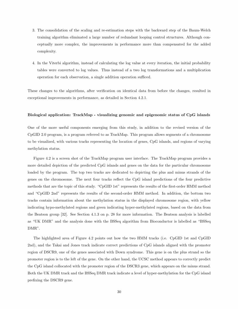
3. The consolidation of the scaling and re-estimation steps with the backward step of the Baum-Welch

training algorithm eliminated a large number of redundant looping control structures. Although con-

ceptually more complex, the improvements in performance more than compensated for the added

complexity.

4. In the Viterbi algorithm, instead of calculating the log value at every iteration, the initial probability

tables were converted to log values. Thus instead of a two log transformations and a multiplication

operation for each observation, a single addition operation sufficed.

These changes to the algorithms, after verification on identical data from before the changes, resulted in

exceptional improvements in performance, as detailed in Section 4.2.1.

Biological application: TrackMap - visualizing genomic and epigenomic status of CpG islands

One of the more useful components emerging from this study, in addition to the revised version of the

CpGID 2.0 program, is a program referred to as TrackMap. This program allows segments of a chromosome

to be visualized, with various tracks representing the location of genes, CpG islands, and regions of varying

methylation status.

Figure 4.2 is a screen shot of the TrackMap program user interface. The TrackMap program provides a

more detailed depiction of the predicted CpG islands and genes on the data for the particular chromosome

loaded by the program. The top two tracks are dedicated to depicting the plus and minus strands of the

genes on the chromosome. The next four tracks reflect the CpG island predictions of the four predictive

methods that are the topic of this study. “CpGID 1st” represents the results of the first-order HMM method

and “CpGID 2nd” represents the results of the second-order HMM method. In addition, the bottom two

tracks contain information about the methylation status in the displayed chromosome region, with yellow

indicating hypo-methylated regions and green indicating hyper-methylated regions, based on the data from

the Beatson group [32]. See Section 4.1.3 on p. 28 for more information. The Beatson analysis is labelled

as “UK DMR” and the analysis done with the BSSeq algorithm from Bioconductor is labelled as “BSSeq

DMR”.

The highlighted area of Figure 4.2 points out how the two HMM tracks (i.e. CpGID 1st and CpGID

2nd), and the Takai and Jones track indicate correct predictions of CpG islands aligned with the promoter

region of DSCR9, one of the genes associated with Down syndrome. This gene is on the plus strand so the

promoter region is to the left of the gene. On the other hand, the UCSC method appears to correctly predict

the CpG island collocated with the promoter region of the DSCR3 gene, which appears on the minus strand.

Both the UK DMR track and the BSSeq DMR track indicate a level of hyper-methylation for the CpG island

prefixing the DSCR9 gene.

30

Figure 4.2: This screenshot of the TrackMap program is typical of the tracks illustrating the genomicand epigenomic information in human chromosomes, in this case chromosome 21. The screen shotshows 2 Mbp segments of the chromosome per screen, and the user may step forward or backwardin 2 Mbp increments. The top two tracks are the plus and minus strands of genes, with gene colorsalternating between red and pink to distinguish between genes in close proximity to each other. Thenext four tracks are CpG island predictions of the four tested prediction methods, starting with afirst-order HMM results track (see Section 5.2.1 on p. 44) and a second-order HMM results track(see Section 5.2.1 on p. 47), then the UCSC predicted CpG islands, and finally the Takai and Jonespredictions. The final two tracks illustrate the differentially methylated regions (DMR) of the IMR90cell line, first by an analysis by the Beatson group, then an analysis performed with the BSSeq softwarefrom Bioconductor. The bottom panel itemizes the genes that appear in the gene tracks, with thegene name lining up vertically with the location on the gene track where the gene appears. The genename appearing in bold face font indicates a significant overlap with some other track feature (suchas a CpG island). Details of the highlighted area are explained in the text.

4.2 Results

4.2.1 Comparison of Hidden Markov Model (HMM) algorithm improvements

with original implementation

Overcoming memory limitations

The original CpGID 1.0 implementation from Spontaneo and Cercone was limited by memory to analyzing

a DNA sequence length of less than 10,000,000 base pairs, quite an unrealistic length when attempting to

characterize a complete human chromosome. The compromise approach needed to characterize a complete

31

chromosome is to partition the sequence into multiple segments and aggregate the analysis from each one.

As has been mentioned, due to logic problems, the original implementation failed to report correct aggregate

totals from the sum of multiple segments.

By converting the core of the implementation to the C# language, revising the algorithm and refactoring

the memory allocation, the current implementation can now quite easily handle a chromosome in excess of

50 million base pairs, as seen in the comparison of Figure 4.3. Much larger volumes of data may be possible.

Figure 4.3: The CpGID 2.0 program has a data volume capacity at least five times greater than theoriginal Spontaneo and Cercone implementation. The right-pointing arrow indicates that a practicalupper limit has not yet been determined.

Overcoming performance limitations

Even short lengths of DNA sequences took an unreasonable length of time to analyze in the original imple-

mentation of the HMM. By altering the algorithm, not only was the run time improved enormously, but any

increase in data length was matched by a linear increase in run time rather than an exponential increase.

Because of the approach taken in implementing the second-order HMM in the revised CpGID 2.0 (see Sec-

tion 5.1.3 on p. 41), this performance gain was realized equally in the second-order implementation of the

HMM.

The original implementation took about nine hours to process the maximum amount of 10 Mbp of data

it could handle. The new version, compared with the original in Figure 4.4, processes the same amount of

data in about ten minutes, an improvement factor of 54 times faster.

As a basis for comparison, running the Takai and Jones software took well over eight hours to run on the

whole of chromosome 21.

32

Figure 4.4: The CpGID 2.0 program is 54 times faster in processing a 10 Mbp DNA segment thanthe original Spontaneo and Cercone implementation.

33

Chapter 5

Impact of initial parameter settings

5.1 Methodology

5.1.1 Issues with genomic data

“hg18” data versus “hg19” data

The hg19 assembly offered by UCSC corresponds to the NBCI Build 37, released as of February 2009. All

things being equal, the hg19 assembly, being the most recent available, would be preferable to the hg18

assembly. Two considerations led to a decision to use hg18 instead:

1. Most documented studies of CpG island prediction are based on the earlier assembly and its annotated

genes. For consistency, this data level was maintained.

2. The epigenetic data received from the Beatson group is based on hg18.

3. There is no simple, linear mapping locations in hg18 to/from locations in hg19.

In order to avoid the need to map addresses between hg18 and hg19, the hg18 assembly was selected as the

reference for this study.

Repeat-masked data and handling unknown nucleotides

Genomic interspersed repeats are large blocks of duplications of DNA bases with no known function, resulting

from copies of DNA segments that have been reintegrated into the genome. Up to 50% of the human genome

is composed of repetitive and low complexity elements, and much of the first third of chromosome 21 is

dominated by such regions. The original Takai and Jones analysis of 2002 was based on data that had

repeats removed by RepeatMasker, a web site and software component dedicated to identifying repeating

regions [41].

34

A complicating factor of these repeating regions is that the GC content in them tends to be higher

than average for the whole genome, leading to the prediction of CpG islands in regions that have no known

functional dependency on the presence of CpG islands. When these low complexity regions cannot be

sequenced, or are identified as repeating elements by RepeatMasker, the nucleotides at those coordinates are

represented as ‘N’ symbols to mask the presence of misleading C and G nucleotides. The effect of applying

this transformation is to reduce the possibility that some CpG islands might be reported as false positives

within a region unrelated to functional genes.

There are two approaches to dealing with these low complexity and repeating regions. The first is to

filter the sequence through the RepeatMasker process. A second approach that is applicable with the hg18

data takes advantage of a convention used by UCSC, the data host. Their approach involves identification

of all low complexity and repeating region sequence data by lower case letters. Thus the ‘A’, ‘C’, ‘G’ and

‘T’ nucleotides in the repeating regions are already identified as ‘a’, ‘c’, ‘g’ and ‘t’ respectively. For the hg18

assembly data, this means a simple transformation of mapping the lower case characters to ‘N’ can produce

a sequence that is effectively repeat-masked. Before the transformation, hg18 already consisted of 13,023,253

nucleotides assigned the ‘N’ value out of a total of 48,129,896 base pairs. These nucleotides represent the 9

Mpb beginning of chromosome 21 and other interspersed regions that have not yet been accurately sequenced.

After the transformation, an additional 16,810,118 nucleotides were assigned the ‘N’ value, leaving 18,296,524

normal base pair values.

The presence of the ‘N’ pseudo-nucleotide, especially its prevalence in the repeat-masked data, begs the

question of how to account for these data in this study. One approach would be to consider ‘N’ as a fifth

observable symbol and build the Markov models to account for this symbol. The other approach is to simply

skip over the ‘N’ nucleotides and treat them as if they do not exist, allowing one to build the Markov model

out of the four standard nucleotides. The one drawback to this approach is that it is conceivable that a

CpG island could be predicted that would span a region that contains ‘N’ observations. In the interest of

simplicity, the second approach was adopted.

5.1.2 Adjusting initial parameter estimates

In order to successfully apply an HMM to a set of serial data, an initial set of transition and emission

probabilities must be specified that are suggestive of the characteristics of the anticipated hidden states of

the model. The training phase of the HMM is expected to produce a revised set of estimated probabilities

that more accurately reflect the properties of the given data. Multiple training iterations are expected

to eventually converge on a set of probabilities that represent the inference of the hidden states from the

observations.

One of the goals of this study was to investigate the impact of the initial set of parameters on the

35

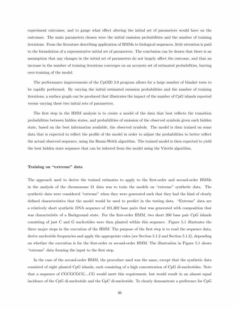
experiment outcomes, and to gauge what effect altering the initial set of parameters would have on the

outcomes. The main parameters chosen were the initial emission probabilities and the number of training

iterations. From the literature describing application of HMMs to biological sequences, little attention is paid

to the formulation of a representative initial set of parameters. The conclusion can be drawn that there is an

assumption that any changes in the initial set of parameters do not largely affect the outcome, and that an

increase in the number of training iterations converges on an accurate set of estimated probabilities, barring

over-training of the model.

The performance improvements of the CpGID 2.0 program allows for a large number of blanket tests to

be rapidly performed. By varying the initial estimated emission probabilities and the number of training

iterations, a surface graph can be produced that illustrates the impact of the number of CpG islands reported

versus varying these two initial sets of parameters.

The first step in the HMM analysis is to create a model of the data that best reflects the transition

probabilities between hidden states, and probabilities of emission of the observed symbols given each hidden

state, based on the best information available, the observed symbols. The model is then trained on some

data that is expected to reflect the profile of the model in order to adjust the probabilities to better reflect

the actual observed sequence, using the Baum-Welch algorithm. The trained model is then expected to yield

the best hidden state sequence that can be inferred from the model using the Viterbi algorithm.

Training on “extreme” data

The approach used to derive the trained estimates to apply to the first-order and second-order HMMs

in the analysis of the chromosome 21 data was to train the models on “extreme” synthetic data. The

synthetic data were considered “extreme” when they were generated such that they had the kind of clearly

defined characteristics that the model would be used to predict in the testing data. “Extreme” data are

a relatively short synthetic DNA sequence of 101,302 base pairs that was generated with composition that

was characteristic of a Background state. For the first-order HMM, two short 200 base pair CpG islands

consisting of just C and G nucleotides were then planted within this sequence. Figure 5.1 illustrates the

three major steps in the execution of the HMM. The purpose of the first step is to read the sequence data,

derive nucleotide frequencies and apply the appropriate rules (see Section 5.1.2 and Section 5.1.2), depending

on whether the execution is for the first-order or second-order HMM. The illustration in Figure 5.1 shows

“extreme” data forming the input to the first step.

In the case of the second-order HMM, the procedure used was the same, except that the synthetic data

consisted of eight planted CpG islands, each consisting of a high concentration of CpG di-nucleotides. Note

that a sequence of CGCGCGCG....CG would meet this requirement, but would result in an almost equal

incidence of the CpG di-nucleotide and the GpC di-nucleotide. To clearly demonstrate a preference for CpG

36

Figure 5.1: A flow diagram showing the steps the CpGID program goes through to predict CpGislands.

di-nucleotides, the CpG island synthetic sequence was set to a repeating set of CGACGCCGGCGT.

The purpose of the second step of Figure 5.1 was to train the model by re-estimating the initial probability

estimates to better reflect the inference of hidden state probabilities from the observed symbols using the

Baum-Welch algorithm. An initial set of probability estimates as described above were then trained against

this “extreme” data set, producing a set of trained probabilities as input in the third step.

The third step used the model parameters produced by the second step to decode the human chromosome

21 data using the Viterbi algorithm. The sequence of hidden states identified by the third step could then

be used to assess the existence of CpG islands in the chromosome data. The program culminated with a

final stage which looked for concentrations of Island states and identified those that satisfy certain criteria

as CpG islands.

Initial estimates for the first-order HMM

For the first-order HMM, an initial set of emission probabilities derived from the nucleotide frequencies of

the data being used for training provided the starting point for the model. The sequence data was read,

and the frequency of the A, C, G and T nucleotides was calculated, and converted to probabilities. For the

repeat-masked copy of chromosome 21, Table 5.1 lists these frequencies and probabilities.

These probabilities could be used for the emission probabilities of both the Background and Island hidden

states, but if the probabilities are the same for both hidden states, there is nothing to distinguish between

them, and once an initial hidden state is inferred, no observed symbol would cause the hidden state to change.

A slight alteration in the initial emission probability estimates is needed to reflect the expectation that the

Background and Island states have different characteristics. That can be done by increasing the probabilities

37

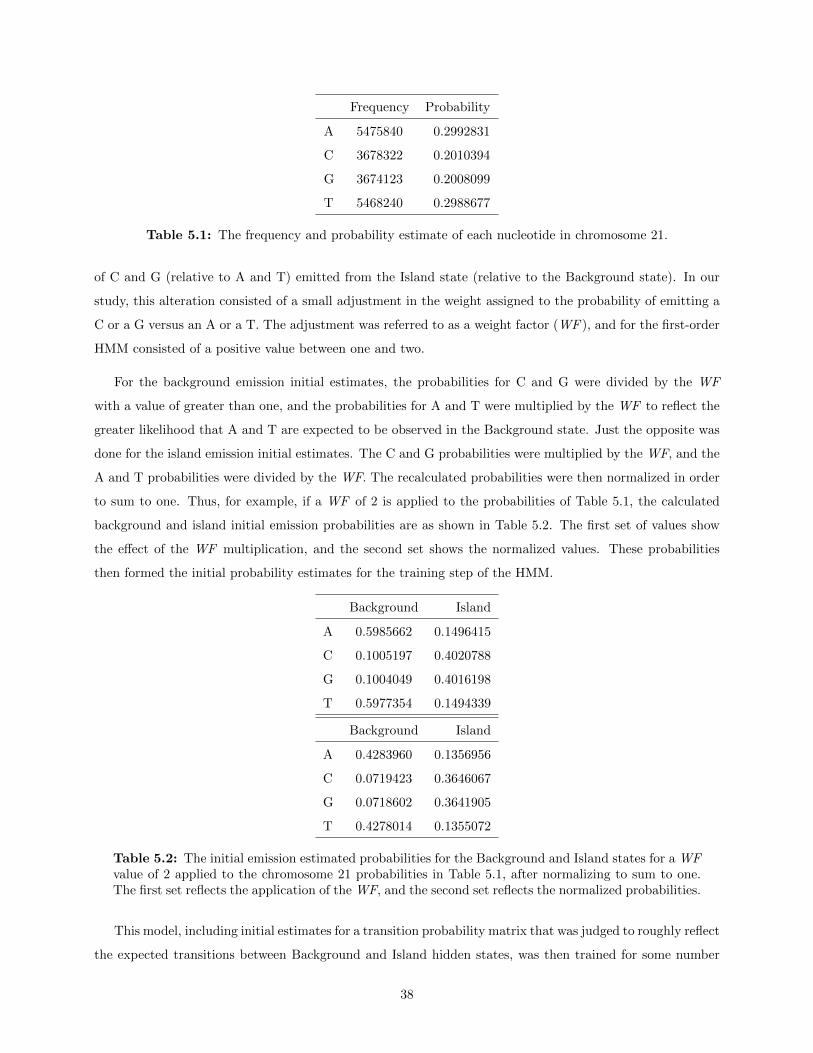
Frequency Probability

A 5475840 0.2992831

C 3678322 0.2010394

G 3674123 0.2008099

T 5468240 0.2988677

Table 5.1: The frequency and probability estimate of each nucleotide in chromosome 21.

of C and G (relative to A and T) emitted from the Island state (relative to the Background state). In our

study, this alteration consisted of a small adjustment in the weight assigned to the probability of emitting a

C or a G versus an A or a T. The adjustment was referred to as a weight factor (WF ), and for the first-order

HMM consisted of a positive value between one and two.

For the background emission initial estimates, the probabilities for C and G were divided by the WF

with a value of greater than one, and the probabilities for A and T were multiplied by the WF to reflect the

greater likelihood that A and T are expected to be observed in the Background state. Just the opposite was

done for the island emission initial estimates. The C and G probabilities were multiplied by the WF, and the

A and T probabilities were divided by the WF. The recalculated probabilities were then normalized in order

to sum to one. Thus, for example, if a WF of 2 is applied to the probabilities of Table 5.1, the calculated

background and island initial emission probabilities are as shown in Table 5.2. The first set of values show

the effect of the WF multiplication, and the second set shows the normalized values. These probabilities

then formed the initial probability estimates for the training step of the HMM.

Background Island

A 0.5985662 0.1496415

C 0.1005197 0.4020788

G 0.1004049 0.4016198

T 0.5977354 0.1494339

Background Island

A 0.4283960 0.1356956

C 0.0719423 0.3646067

G 0.0718602 0.3641905

T 0.4278014 0.1355072

Table 5.2: The initial emission estimated probabilities for the Background and Island states for a WFvalue of 2 applied to the chromosome 21 probabilities in Table 5.1, after normalizing to sum to one.The first set reflects the application of the WF, and the second set reflects the normalized probabilities.

This model, including initial estimates for a transition probability matrix that was judged to roughly reflect

the expected transitions between Background and Island hidden states, was then trained for some number

38

of iterations of the Baum-Welch algorithm on “extreme” data, as described in Section 5.1.2. Each training

iteration started with the revised model of estimated probabilities from the previous training iteration.

The resulting set of probabilities was tested against a sequence of observed data such as chromosome 21

to determine the best sequence of hidden states that can be inferred from the probabilities. This sequence

of hidden states was then used to assess the frequency and size of CpG islands within that sequence.

In our study, the first-order HMM model parameters were altered, re-trained and tested repeatedly against

the same data with two alterations. The first change was in the number of iterations used in the training

process. The second change was in the value of the WF applied to the initial emission probability estimates.

The effect of each combination of changes could then be measured in the reported outcome of the test, which

in our case was the number of CpG islands predicted.

Initial estimates for the second-order HMM

For the second-order HMM, instead of the nucleotide frequencies, the frequencies of interest are the di-

nucleotide frequencies. The entire repeat-masked chromosome 21 was analyzed to determine the frequency

of each di-nucleotide observation. These frequencies were recorded and converted into probability estimates

as in Table 5.3. The probabilities for all sixteen grid elements total one by definition.

Initial probabilities A C G T

A 0.1055968 0.0534439 0.0715261 0.0843868

C 0.0697866 0.0491981 0.0106345 0.0668795

G 0.0575206 0.0408264 0.0490688 0.0488661

T 0.0663791 0.0575709 0.0695805 0.0987352

Table 5.3: The probability of each di-nucleotide occurring in chromosome 21, based on observedfrequencies of each di-nucleotide. The bold highlight illustrates the CpG di-nucleotide (a C from therows and a G from the columns).

The original probabilities were transformed into initial Background and Island estimated probabilities by

applying a weight factor WF (where WF is a fractional value between zero and one) to each probability

according to the rules in Table 5.4. The rules are structured so as to yield a greater propensity for the

di-nucleotides including C and G in the Island state, particularly the CpG di-nucleotide.

After applying the WF rules, the new fractions were normalized by dividing each table element for the

Background fractions by the sum of the entire Background table to ensure that the sum of the probabilities

for each of the sixteen elements total one. The same procedure was applied to the Island table portion of

Table 5.4.

To illustrate, suppose WF = 0.2. Table 5.5 illustrates the probability values for each di-nucleotide after

39

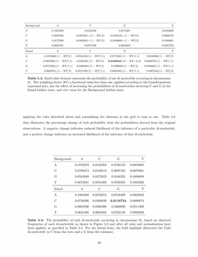
Background A C G T

A 0.1055968 0.0534439 0.0715261 0.0843868

C 0.0697866 0.0491981 ∗ (1−WF/2) 0.0106345 ∗ (1−WF/2) 0.0668795

G 0.0575206 0.0408264 ∗ (1−WF/2) 0.0490688 ∗ (1−WF/2) 0.0488661

T 0.0663791 0.0575709 0.0695805 0.0987352

Island A C G T

A 0.1055968/(1−WF/2) 0.0534439/(1−WF/1.1) 0.0715261/(1−WF/1.1) 0.0843868/(1−WF/2)

C 0.0697866/(1−WF/1.1) 0.0491981/(1−WF/2) 0.0106345/(1−WF ∗ 1.1) 0.0668795/(1−WF/1.1)

G 0.0575206/(1−WF/1.1) 0.0408264/(1−WF/2) 0.0490688/(1−WF/2) 0.0488661/(1−WF/1.1)

T 0.0663791/(1−WF/2) 0.0575709/(1−WF/1.1) 0.0695805/(1−WF/1.1) 0.0987352/(1−WF/2)

Table 5.4: Each table element represents the probability of one di-nucleotide occurring in chromosome21. The weighting factor WF, a fractional value less than one, applied according to the transformationsexpressed here, has the effect of increasing the probabilities of di-nucleotides involving C and G in theIsland hidden state, and vice versa for the Background hidden state.

applying the rules described above and normalizing the elements in the grid to sum to one. Table 5.6

then illustrates the percentage change of each probability from the probabilities derived from the original

observations. A negative change indicates reduced likelihood of the inference of a particular di-nucleotide,

and a positive change indicates an increased likelihood of the inference of that di-nucleotide.

Background A C G T

A 0.1072019 0.0542563 0.0726133 0.0856695

C 0.0708474 0.0449513 0.0097165 0.0678961

G 0.0583949 0.0373023 0.0448332 0.0496089

T 0.0673881 0.0584460 0.0706382 0.1002360

Island A C G T

A 0.1004580 0.0559274 0.0748499 0.0802802

C 0.0730296 0.0468039 0.0116734 0.0699874

G 0.0601936 0.0388396 0.0466809 0.0511369

T 0.0631488 0.0602462 0.0728139 0.0939303

Table 5.5: The probability of each di-nucleotide occurring in chromosome 21, based on observedfrequencies of each di-nucleotide as shown in Figure 5.3 and after all rules and normalization havebeen applied, as specified in Table 5.4. For the Island state, the bold highlight illustrates the CpGdi-nucleotide (a C from the rows and a G from the columns).

40

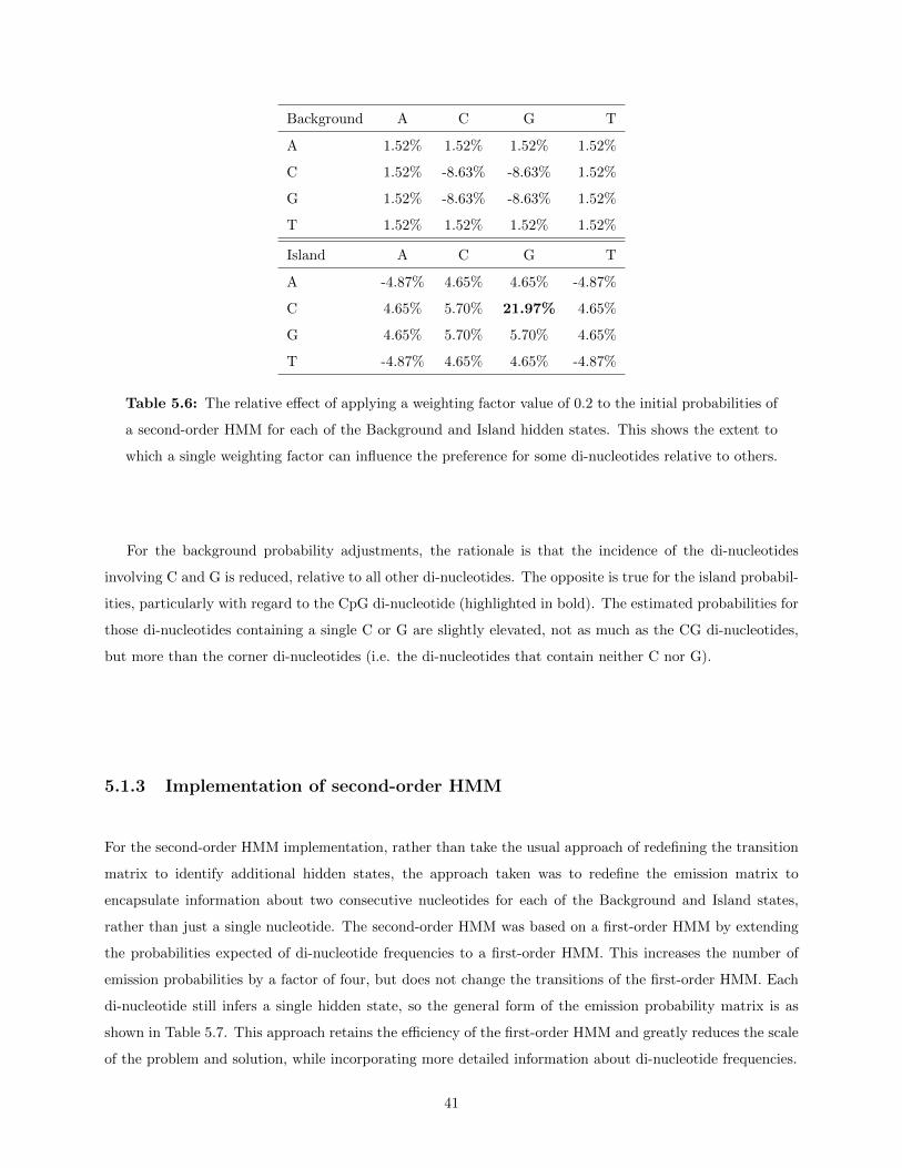
Background A C G T

A 1.52% 1.52% 1.52% 1.52%

C 1.52% -8.63% -8.63% 1.52%

G 1.52% -8.63% -8.63% 1.52%

T 1.52% 1.52% 1.52% 1.52%

Island A C G T

A -4.87% 4.65% 4.65% -4.87%

C 4.65% 5.70% 21.97% 4.65%

G 4.65% 5.70% 5.70% 4.65%

T -4.87% 4.65% 4.65% -4.87%

Table 5.6: The relative effect of applying a weighting factor value of 0.2 to the initial probabilities of

a second-order HMM for each of the Background and Island hidden states. This shows the extent to

which a single weighting factor can influence the preference for some di-nucleotides relative to others.

For the background probability adjustments, the rationale is that the incidence of the di-nucleotides

involving C and G is reduced, relative to all other di-nucleotides. The opposite is true for the island probabil-

ities, particularly with regard to the CpG di-nucleotide (highlighted in bold). The estimated probabilities for

those di-nucleotides containing a single C or G are slightly elevated, not as much as the CG di-nucleotides,

but more than the corner di-nucleotides (i.e. the di-nucleotides that contain neither C nor G).

5.1.3 Implementation of second-order HMM

For the second-order HMM implementation, rather than take the usual approach of redefining the transition

matrix to identify additional hidden states, the approach taken was to redefine the emission matrix to

encapsulate information about two consecutive nucleotides for each of the Background and Island states,

rather than just a single nucleotide. The second-order HMM was based on a first-order HMM by extending

the probabilities expected of di-nucleotide frequencies to a first-order HMM. This increases the number of

emission probabilities by a factor of four, but does not change the transitions of the first-order HMM. Each

di-nucleotide still infers a single hidden state, so the general form of the emission probability matrix is as

shown in Table 5.7. This approach retains the efficiency of the first-order HMM and greatly reduces the scale

of the problem and solution, while incorporating more detailed information about di-nucleotide frequencies.

41

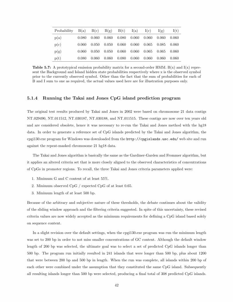
Probability B(a) B(c) B(g) B(t) I(a) I(c) I(g) I(t)

p(a) 0.080 0.060 0.060 0.080 0.060 0.060 0.060 0.060

p(c) 0.060 0.050 0.050 0.060 0.060 0.065 0.085 0.060

p(g) 0.060 0.050 0.050 0.060 0.060 0.065 0.065 0.060

p(t) 0.080 0.060 0.060 0.080 0.060 0.060 0.060 0.060

Table 5.7: A prototypical emission probability matrix for a second-order HMM. B(x) and I(x) repre-sent the Background and Island hidden state probabilities respectively where x is the observed symbolprior to the currently observed symbol. Other than the fact that the sum of probabilities for each ofB and I sum to one as required, the actual values used here are for illustration purposes only.

5.1.4 Running the Takai and Jones CpG island prediction program

The original test results produced by Takai and Jones in 2002 were based on chromosome 21 data contigs

NT 029490, NT 011512, NT 030187, NT 030188, and NT 011515. These contigs are now over ten years old

and are considered obsolete, hence it was necessary to re-run the Takai and Jones method with the hg18

data. In order to generate a reference set of CpG islands predicted by the Takai and Jones algorithm, the

cpgi130.exe program for Windows was downloaded from the http://cpgislands.usc.edu/ web site and run

against the repeat-masked chromosome 21 hg18 data.

The Takai and Jones algorithm is basically the same as the Gardiner-Garden and Frommer algorithm, but

it applies an altered criteria set that is more closely aligned to the observed characteristics of concentrations

of CpGs in promoter regions. To recall, the three Takai and Jones criteria parameters applied were:

1. Minimum G and C content of at least 55%.

2. Minimum observed CpG / expected CpG of at least 0.65.

3. Minimum length of at least 500 bp.

Because of the arbitrary and subjective nature of these thresholds, the debate continues about the validity

of the sliding window approach and the filtering criteria suggested. In spite of this uncertainty, these revised

criteria values are now widely accepted as the minimum requirements for defining a CpG island based solely

on sequence content.

In a slight revision over the default settings, when the cpgi130.exe program was run the minimum length

was set to 200 bp in order to not miss smaller concentrations of GC content. Although the default window

length of 200 bp was selected, the ultimate goal was to select a set of predicted CpG islands longer than

500 bp. The program run initially resulted in 241 islands that were longer than 500 bp, plus about 1200

that were between 200 bp and 500 bp in length. When the run was complete, all islands within 200 bp of

each other were combined under the assumption that they constituted the same CpG island. Subsequently

all resulting islands longer than 500 bp were selected, producing a final total of 308 predicted CpG islands.

42

These were the predictions used to subsequently compare with the other methods.

5.1.5 Method of comparison of CpG island predictions

Four prediction methods were compared in this test, comprising the Takai and Jones method, the first-order

HMM method, the second-order HMM method and the UCSC method. Each of the prediction methods

produced a list of CpG islands together with their location and length within human chromosome 21. This

list was compared with the locations of known genes in chromosome 21. The measure used in this test was

the accuracy and sensitivity of the association between predicted CpG islands and their associated genes.

The use of these metrics must be tempered with the knowledge that the association between genes and

CpG islands in their promoter regions is much less than 100%. The assumption that each gene has one

upstream promoter, and that this promoter collocates with a CpG island, is not necessarily true; plenty of

counter-examples exist.

In order to evaluate the association between CpG islands and the promoter regions of genes that have been

identified and annotated for chromosome 21, an upstream region threshold of 5000 base pairs was defined.

If the predicted CpG island start fell anywhere within the 5000 base pairs upstream of any gene, this was

considered to be a true positive (TP). This range is suggested by Aston et al. [3], and is large enough to

possibly encompass some enhancer regions which may also be influenced by the presence of CpG islands.

The CpG island region was also allowed to overlap with the transcription start site at the beginning of the

gene by up to 500 base pairs. All other predicted CpG islands that fell outside of these boundaries, even if

they qualified as CpG islands according to the Takai and Jones criteria, were designated as false positives

(FP). Known gene promoters that were not included in the CpG island predictions were designated as false

negatives (FN).

To quantify the accuracy of predicted CpG islands based on these values, and to provide a means of

comparing different methods, the following definitions apply:

1. Collocated with genes (TP)

2. Not collocated with genes (FP)

3. Genes with no island predicted (FN)

4. Total predicted CpG islands (TP+FP)

5. Sensitivity [TP/(TP+FN)]

6. Accuracy / Positive Predictive Value (PPV) [TP/(TP+FP)]

7. False Discovery Rate (FDR) (1 - PPV)

One way of gauging the efficacy of the prediction methods, based on the criteria of Takai and Jones, is to

measure and compare the CG content and observed versus expected CpG incidence of each predicted CpG

43

island. Since this is the only basis of selection for the Takai and Jones method and the HMM methods, these

methods are expected to score well. The UCSC method of prediction is based on epigenomic factors such

as DNA methylation, frequent promoter activity and open chromatin structure as reported by Christopher

Bock [6], and CG content is only one consideration out of many. Comparing the CG characteristics of the first

three methods with the UCSC methods, especially in those CpG islands that are not predicted in common,

should shed light on the efficacy of each method.

Another means of assessing the accuracy of the CpG island predictions is to examine the promoter region

of each gene on chromosome 21, and categorize them based on CG content and their prediction status of

each of the four prediction methods. The following approach was used to perform this assessment:

1. For each identified gene in the hg18 sequence, examine the DNA region 5000 base pairs upstream of

the gene start address, including up to 500 base pairs coincident with the start of the gene. The length

of the promoter region may be smaller than 5500 base pairs to the extent that the gene itself is smaller

than the 500 base pairs that the promoter region is suggested as intruding into the gene start region.

This is relevant primarily in genes where the coding sequence is not yet known or is incomplete.

2. Tabulate the CG content percentage and CpG observed/expected ratio for each gene promoter region.

3. Rank the genes by these statistics to identify the number of genes that would be expected to be identified

by a prediction method based on DNA sequence content.

4. Relate the CpG island predictions of the second-order HMM to the resulting gene prediction list to

assess the efficacy of the second-order HMM method.

This approach makes a possibly unrealistic assumption that the upstream portion of the promoter regions

are of a uniform size. Also CpG islands within this promoter region are expected to be much smaller than

the region itself, with characteristically higher CG content percentage and CpG observed/expected ratio

values than the overall region. As a result, the average CG content and ratio scores of the promoter regions

themselves would be expected to be lower overall than the CpG island(s) they contain.

5.2 Results

5.2.1 Impact of initial parameter estimates on prediction outcomes

First-order HMM

One of the most important findings of this study is that HMM outcomes are highly dependent on the initial

probability estimates and do not necessarily converge on a common set of predictions. Predicted outcomes are

44

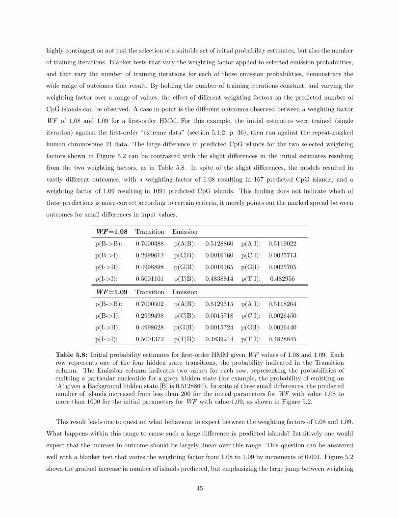
highly contingent on not just the selection of a suitable set of initial probability estimates, but also the number

of training iterations. Blanket tests that vary the weighting factor applied to selected emission probabilities,

and that vary the number of training iterations for each of those emission probabilities, demonstrate the

wide range of outcomes that result. By holding the number of training iterations constant, and varying the

weighting factor over a range of values, the effect of different weighting factors on the predicted number of

CpG islands can be observed. A case in point is the different outcomes observed between a weighting factor

WF of 1.08 and 1.09 for a first-order HMM. For this example, the initial estimates were trained (single

iteration) against the first-order “extreme data” (section 5.1.2, p. 36), then run against the repeat-masked

human chromosome 21 data. The large difference in predicted CpG islands for the two selected weighting

factors shown in Figure 5.2 can be contrasted with the slight differences in the initial estimates resulting

from the two weighting factors, as in Table 5.8. In spite of the slight differences, the models resulted in

vastly different outcomes, with a weighting factor of 1.08 resulting in 167 predicted CpG islands, and a

weighting factor of 1.09 resulting in 1091 predicted CpG islands. This finding does not indicate which of

these predictions is more correct according to certain criteria, it merely points out the marked spread between

outcomes for small differences in input values.

WF=1.08 Transition Emission

p(B->B): 0.7000388 p(A|B): 0.5128860 p(A|I): 0.5119022

p(B->I): 0.2999612 p(C|B): 0.0016160 p(C|I): 0.0025713

p(I->B): 0.4998898 p(G|B): 0.0016165 p(G|I): 0.0025705

p(I->I): 0.5001101 p(T|B): 0.4838814 p(T|I): 0.482956

WF=1.09 Transition Emission

p(B->B): 0.7000502 p(A|B): 0.5129315 p(A|I): 0.5118264

p(B->I): 0.2999498 p(C|B): 0.0015718 p(C|I): 0.0026450

p(I->B): 0.4998628 p(G|B): 0.0015724 p(G|I): 0.0026440

p(I->I): 0.5001372 p(T|B): 0.4839244 p(T|I): 0.4828845

Table 5.8: Initial probability estimates for first-order HMM given WF values of 1.08 and 1.09. Eachrow represents one of the four hidden state transitions, the probability indicated in the Transitioncolumn. The Emission column indicates two values for each row, representing the probabilities ofemitting a particular nucleotide for a given hidden state (for example, the probability of emitting an‘A’ given a Background hidden state [B] is 0.5128860). In spite of these small differences, the predictednumber of islands increased from less than 200 for the initial parameters for WF with value 1.08 tomore than 1000 for the initial parameters for WF with value 1.09, as shown in Figure 5.2.

This result leads one to question what behaviour to expect between the weighting factors of 1.08 and 1.09.

What happens within this range to cause such a large difference in predicted islands? Intuitively one would

expect that the increase in outcome should be largely linear over this range. This question can be answered

well with a blanket test that varies the weighting factor from 1.08 to 1.09 by increments of 0.001. Figure 5.2

shows the gradual increase in number of islands predicted, but emphasizing the large jump between weighting

45

factors with values of 1.087 and 1.088. This same result could be examined further to explore the nature

of the increase within the range of 1.087 and 1.088, as shown in Figure 5.3. This general result occurred

repeatedly over many blanket tests using different weighting factor ranges, confirming that this is a common

behaviour of the HMM.

Figure 5.2: The number of CpG islands predicted by the first-order HMM jumps rapidly with WFvalues between 1.087 and 1.088 and number of training iterations held constant at one, then increasesmore gradually.

For all these tests the number of training iterations was held constant at one. Again, the predominant

part of the jump in predicted islands from roughly 500 for a weighting factor value of 1.087 to more than

1000 for a weighting factor value of 1.088 in Figure 5.3 occurred within a small range of weighting factors

values, between 1.0873 and 1.0875. On either side of that window, the increase in the number of predicted

islands is relatively gradual. Table 5.9 shows the model parameters derived from the two weighting factor

values of 1.0873 and 1.0874, and the minuscule differences between the two.

In order to assess the impact of multiple training iterations for various weighting factor values on number

of predicted islands, up to five training iterations were evaluated on each weighting factor from 1.075 to

1.080 with an increment of 0.001. The surface graph (Figure 5.4) corresponding to this test shows that

each training iteration resulted in a large increase in number of islands predicted regardless of the starting

probability estimates.

Each training iteration rapidly increased the number of predicted CpG islands by increments of roughly

1000, topping out at the artificial cutoff of 4000. The increase in number of predicted islands was much

greater for each training iteration than any increase between weighting factor values.

46

Figure 5.3: The number of islands predicted jumps rapidly between weighting factors with values1.0873 and 1.0875 and number of training iterations held constant at one, then increases more gradually.

Second-order HMM

The second-order HMM results can be illustrated with a similar approach as for the first-order HMM. Using

the second-order “extreme data” sample as a training base (section 5.1.2, p. 36), the lowest weighting factor

that successfully identified all fourteen CpG islands was 0.63.

The second-order HMM exhibits a much more gradual increase in number of islands predicted in chromo-

some 21 with increasing weighting factor values. In a blanket test with weighting factor values varying from

0.5 to 0.8 by increments of 0.01 with one training iteration (Figure 5.5), the increase in number of islands

shows some short ranges of weighting factor that have a steeper rate of increase than others. Table 5.10

compares just the emission probabilities of the two weighting factors, 0.76 and 0.77, and illustrates how little

difference there is between the two, yet there is about a 20% increase in the predicted number of CpG islands.

The anomalous behaviour is not as dramatic as for the first-order HMM, but is evidently not linear for some

ranges of input parameters.

Figure 5.6 is a surface graph to illustrate the topography of the second-order HMM resulting for weighting

factor values from 0.60 to 0.67, with up to five training iterations. Table 5.11 presents the data underlying

the surface graph of Figure 5.6.

One of the CpG island predictions expected to align best with the number of gene promoter regions

on chromosome 21 is the 335 islands predicted by a WF=0.65 with three training iterations. A closer

47

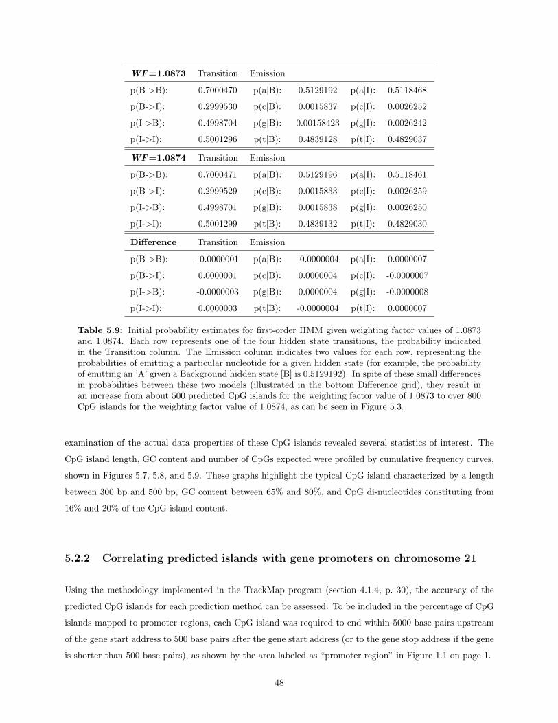
WF=1.0873 Transition Emission

p(B->B): 0.7000470 p(a|B): 0.5129192 p(a|I): 0.5118468

p(B->I): 0.2999530 p(c|B): 0.0015837 p(c|I): 0.0026252

p(I->B): 0.4998704 p(g|B): 0.00158423 p(g|I): 0.0026242

p(I->I): 0.5001296 p(t|B): 0.4839128 p(t|I): 0.4829037

WF=1.0874 Transition Emission

p(B->B): 0.7000471 p(a|B): 0.5129196 p(a|I): 0.5118461

p(B->I): 0.2999529 p(c|B): 0.0015833 p(c|I): 0.0026259

p(I->B): 0.4998701 p(g|B): 0.0015838 p(g|I): 0.0026250

p(I->I): 0.5001299 p(t|B): 0.4839132 p(t|I): 0.4829030

Difference Transition Emission

p(B->B): -0.0000001 p(a|B): -0.0000004 p(a|I): 0.0000007

p(B->I): 0.0000001 p(c|B): 0.0000004 p(c|I): -0.0000007

p(I->B): -0.0000003 p(g|B): 0.0000004 p(g|I): -0.0000008

p(I->I): 0.0000003 p(t|B): -0.0000004 p(t|I): 0.0000007

Table 5.9: Initial probability estimates for first-order HMM given weighting factor values of 1.0873and 1.0874. Each row represents one of the four hidden state transitions, the probability indicatedin the Transition column. The Emission column indicates two values for each row, representing theprobabilities of emitting a particular nucleotide for a given hidden state (for example, the probabilityof emitting an ’A’ given a Background hidden state [B] is 0.5129192). In spite of these small differencesin probabilities between these two models (illustrated in the bottom Difference grid), they result inan increase from about 500 predicted CpG islands for the weighting factor value of 1.0873 to over 800CpG islands for the weighting factor value of 1.0874, as can be seen in Figure 5.3.

examination of the actual data properties of these CpG islands revealed several statistics of interest. The

CpG island length, GC content and number of CpGs expected were profiled by cumulative frequency curves,

shown in Figures 5.7, 5.8, and 5.9. These graphs highlight the typical CpG island characterized by a length

between 300 bp and 500 bp, GC content between 65% and 80%, and CpG di-nucleotides constituting from

16% and 20% of the CpG island content.

5.2.2 Correlating predicted islands with gene promoters on chromosome 21

Using the methodology implemented in the TrackMap program (section 4.1.4, p. 30), the accuracy of the

predicted CpG islands for each prediction method can be assessed. To be included in the percentage of CpG

islands mapped to promoter regions, each CpG island was required to end within 5000 base pairs upstream

of the gene start address to 500 base pairs after the gene start address (or to the gene stop address if the gene

is shorter than 500 base pairs), as shown by the area labeled as “promoter region” in Figure 1.1 on page 1.

48

Figure 5.4: A first-order HMM surface graph showing the number of CpG islands predicted whenthe weighting factor value ranges from 1.075 in steps of .001 to 1.080, and the number of trainingiterations varies from one to five for each of those weight factor values. The increase in number ofislands predicted is dominated by increasing training iterations rather than increasing weighting factorvalues. It appears that over-training occurs rapidly with increased number of training iterations.

The four prediction methods are the Takai and Jones windowing method, the CpGID first-order HMM,

the CpGID second-order HMM, and the UCSC CpG island map. The first-order HMM test generated a

prediction of 359 CpG islands when tested on chromosome 21 data, based on a weighting factor value of

1.084 and one training iteration trained on “extreme” data. The second-order HMM test, using a similar

approach, generated a prediction of 335 CpG islands, based on a weighting factor value of 0.65 and three

training iterations. These prediction counts of CpG islands were judged to be indicative of the number of

islands expected in relation to the gene count of chromosome 21. The percentage of islands mapped to a

region upstream of a gene for these four prediction methods is given in Table 5.12. A detailed examination

of the CpG islands predicted by each of the four methods suggested that the UCSC method is quite disjoint

from the predictions of the other three methods, as only ten islands are shared between the UCSC method

and all three other methods combined.

Table 5.13 lists the top 10 genes in chromosome 21 in order of CpG observed/expected ratio, as outlined

in the above approach. Since the CpG observed/expected ratio and the CG% content are not independent,

49

Figure 5.5: The predicted number of CpG islands for a second-order HMM for a range of weightingfactor values.

the CG% content and CpG observed/expected ratio are expected to be correlated in their ranking.

Table 5.14 lists the top 10 genes in chromosome 21 in order of CG content percentage, as outlined in the

above approach. There is some degree of overlap between the two top 10 lists, as expected there would be.

Table 5.15 lists the twenty CpG islands predicted in chromosome 21 by the second-order HMM method.

The focus on the comparison of the HMM methods with the UCSC and Takai and Jones methods of CpG

island prediction and identification has served to show that the HMM methods can perform well relative to

each other in terms of accuracy and sensitivity. The fact of the matter is that none of the methods came

particularly close to predicting the expected number of CpG islands coincident with promoter regions of

genes, pointing out the importance of specifying a suitable set of predictive criteria. Some satisfaction was

gained in that the second-order HMM was successful in incorporating the additional information available to

achieve results that were better than the first-order HMM.

However, this comparison provided the backdrop for pointing out the sensitivity of the HMM outcomes,

particularly the first-order HMM, to the settings of the initial estimates of the model parameters. Small

differences at certain points along a range of input probabilities produced incongruent increases in the number

of CpG island states. Even greater increases in prediction counts were seen when increasing numbers of

training iterations were applied. Although the exact explanation for this phenomenon is unknown, the

realization of this behaviour points out the need for careful assessment of the results produced by HMMs.

50

WF=.76 B: a c g t

a 0.0963448 0.0669691 0.5118468 0.5004150

c 0.0646814 0.0419308 0.0344291 0.0616421

g 0.0648642 0.0390768 0.0374151 0.0592262

t 0.0841654 0.0630872 0.0577429 0816958

WF=.76 I: a c g t

a 0.0391918 0.0640915 0.0584654 0.0342817

c 0.0601779 0.0957703 0.1124759 0.0575586

g 0.0623297 0.0915182 0.0851266 0.0569598

t 0.0343035 0.0605332 0.0539236 0.0539236

WF=.77 B: a c g t

a 0.0968310 0.0670406 0.0627097 0.0845400

c 0.0647817 0.0414548 0.0334157 0.0617361

g 0.0649304 0.0385985 0.0369929 0.0592860

t 0.0845905 0.0631529 0.0578309 0.0821085

WF=.77 I: a c g t

a 0.0382422 0.0639645 0.0582949 0.0334526

c 0.0599986 0.0966949 0.1143610 0.0573910

g 0.0622124 0.0924435 0.0859467 0.0568538

t 0.0334735 0.0604168 0.0537667 0.0537667

Difference B: a c g t

a -0.0004862 -0.0000715 -0.0000956 -0.0004247

c -0.0001003 0.0004760 0.0010134 -0.0000941

g -0.0000662 0.0004783 0.0004221 -0.0000598

t -0.0004251 -0.0000657 -0.0000880 -0.0004127

Difference I: a c g t

a 0.0009496 0.0001270 0.0001705 0.0008291

c 0.0001793 -0.0009246 -0.0018851 0.0001676

g 0.0001173 -0.0009253 -0.0008201 0.0001060

t 0.0008300 0.0001164 0.0001569 0.0001569

Table 5.10: Initial probability estimates for second-order HMM given weighting factor values of 0.76and 0.77. Although not as pronounced as the first-order HMM case, the bottom Difference sectionagain illustrates the miniscule emission probability differences between the two models. These smalldifferences still result in a large jump in the number of predicted CpG islands, as shown in Figure 5.5.

51

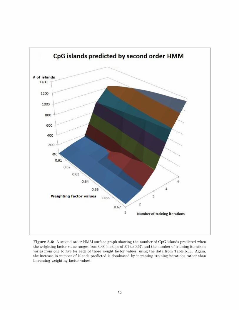
Figure 5.6: A second-order HMM surface graph showing the number of CpG islands predicted whenthe weighting factor value ranges from 0.60 in steps of .01 to 0.67, and the number of training iterationsvaries from one to five for each of those weight factor values, using the data from Table 5.11. Again,the increase in number of islands predicted is dominated by increasing training iterations rather thanincreasing weighting factor values.

52

Iteration WF=0.60 WF=0.61 WF=0.62 WF=0.63 WF=0.64 WF=0.65 WF=0.66 WF=0.67

1: 18 28 35 36 43 49 52 56

2: 105 114 115 117 124 126 137 151

3: 163 169 188 213 314 335 399 409

4: 766 822 851 879 905 938 954 978

5: 1032 1112 1169 1222 1268 1301 1328 1359

Table 5.11: Predicted CpG island counts on chromosome 21 for second-order HMM with weightingfactor values ranging from 0.60 to 0.67 and training iterations ranging from one to five. These datavalues are illustrated in Figure 5.6.

Figure 5.7: The frequency profile of CpG island lengths as identified by the second-order HMM onchromosome 21. The greatest frequency of CpG island length occurs between 300 bp and 500 bp.

Method Percentage

Takai and Jones: 5.54%

First-order HMM: 5.57%

Second-order HMM: 6.57%

UCSC: 18.59%

Table 5.12: Percentage of CpG islands mapped to gene promoters in chromosome 21 for each of thefour prediction methods.

53

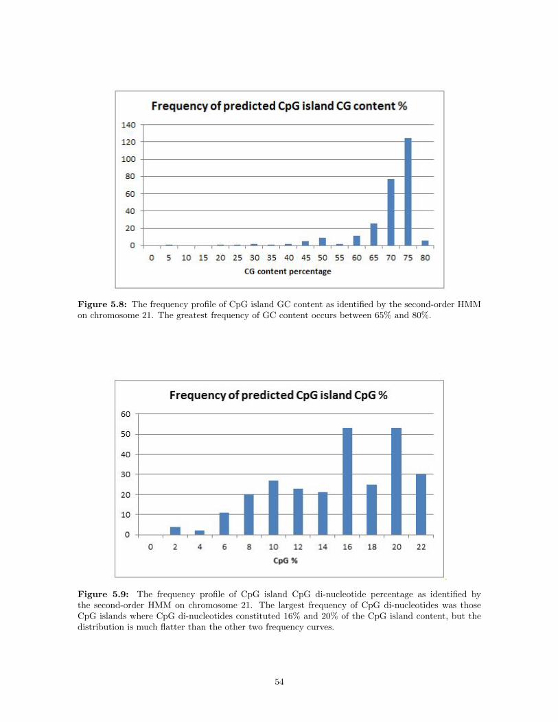
Figure 5.8: The frequency profile of CpG island GC content as identified by the second-order HMMon chromosome 21. The greatest frequency of GC content occurs between 65% and 80%.

Figure 5.9: The frequency profile of CpG island CpG di-nucleotide percentage as identified bythe second-order HMM on chromosome 21. The largest frequency of CpG di-nucleotides was thoseCpG islands where CpG di-nucleotides constituted 16% and 20% of the CpG island content, but thedistribution is much flatter than the other two frequency curves.

54

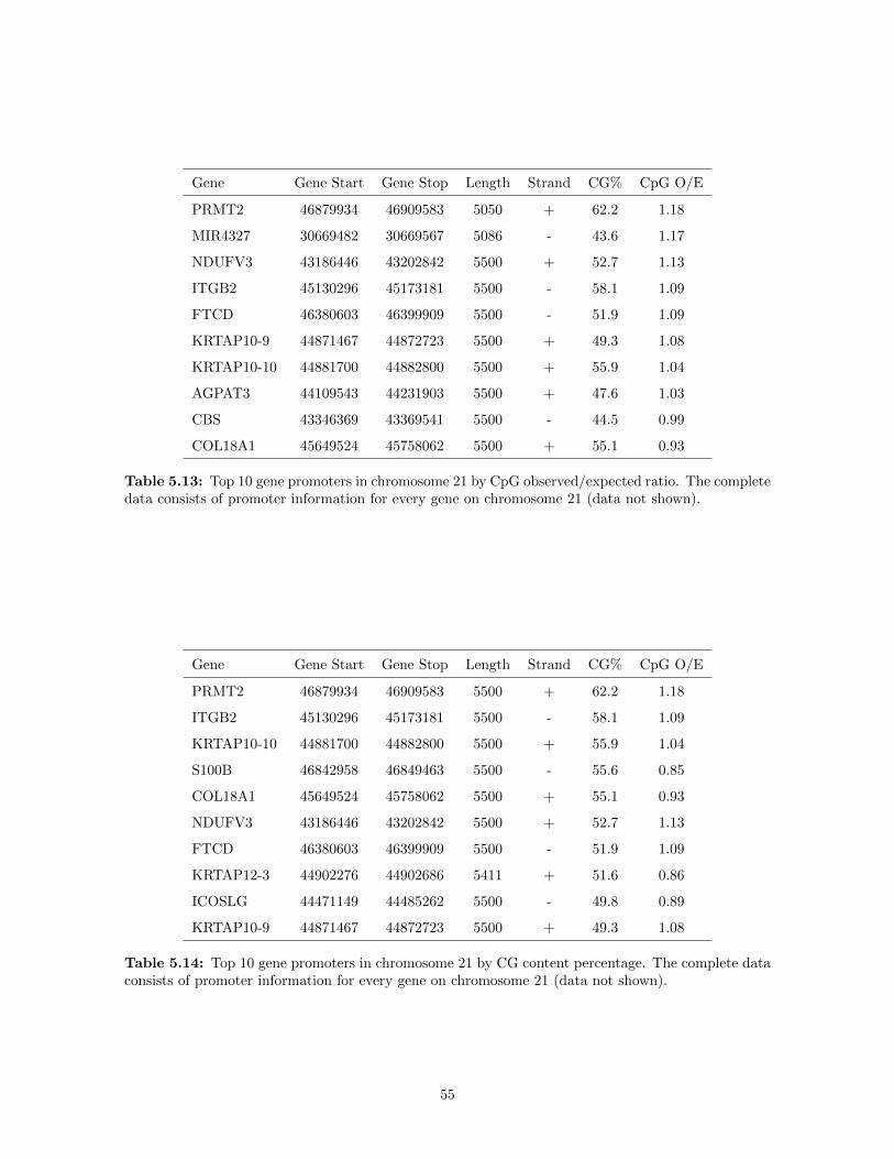
Gene Gene Start Gene Stop Length Strand CG% CpG O/E

PRMT2 46879934 46909583 5050 + 62.2 1.18

MIR4327 30669482 30669567 5086 - 43.6 1.17

NDUFV3 43186446 43202842 5500 + 52.7 1.13

ITGB2 45130296 45173181 5500 - 58.1 1.09

FTCD 46380603 46399909 5500 - 51.9 1.09

KRTAP10-9 44871467 44872723 5500 + 49.3 1.08

KRTAP10-10 44881700 44882800 5500 + 55.9 1.04

AGPAT3 44109543 44231903 5500 + 47.6 1.03

CBS 43346369 43369541 5500 - 44.5 0.99

COL18A1 45649524 45758062 5500 + 55.1 0.93

Table 5.13: Top 10 gene promoters in chromosome 21 by CpG observed/expected ratio. The completedata consists of promoter information for every gene on chromosome 21 (data not shown).

Gene Gene Start Gene Stop Length Strand CG% CpG O/E

PRMT2 46879934 46909583 5500 + 62.2 1.18

ITGB2 45130296 45173181 5500 - 58.1 1.09

KRTAP10-10 44881700 44882800 5500 + 55.9 1.04

S100B 46842958 46849463 5500 - 55.6 0.85

COL18A1 45649524 45758062 5500 + 55.1 0.93

NDUFV3 43186446 43202842 5500 + 52.7 1.13

FTCD 46380603 46399909 5500 - 51.9 1.09

KRTAP12-3 44902276 44902686 5411 + 51.6 0.86

ICOSLG 44471149 44485262 5500 - 49.8 0.89

KRTAP10-9 44871467 44872723 5500 + 49.3 1.08

Table 5.14: Top 10 gene promoters in chromosome 21 by CG content percentage. The complete dataconsists of promoter information for every gene on chromosome 21 (data not shown).

55

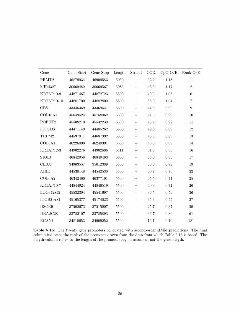
Gene Gene Start Gene Stop Length Strand CG% CpG O/E Rank O/E

PRMT2 46879934 46909583 5050 + 62.2 1.18 1

MIR4327 30669482 30669567 5086 - 43.6 1.17 2

KRTAP10-9 44871467 44872723 5500 + 49.3 1.08 6

KRTAP10-10 44881700 44882800 5500 + 55.9 1.04 7

CBS 43346369 43369541 5500 - 44.5 0.99 9

COL18A1 45649524 45758062 5500 - 44.5 0.99 10

POFUT2 45508270 45532239 5500 - 46.4 0.92 11

ICOSLG 44471149 44485262 5500 - 49.8 0.89 12

TRPM2 44597911 44687392 5500 + 46.5 0.89 13

COL6A1 46226090 46249391 5500 + 46.5 0.89 14

KRTAP12-3 44902276 44902686 5411 + 51.6 0.86 16

S100B 46842958 46849463 5500 - 55.6 0.85 17

CLIC6 34963557 35012389 5500 + 36.3 0.83 19

AIRE 44530148 44542530 5500 + 30.7 0.76 22

COL6A2 46342460 46377191 5500 + 45.5 0.71 25

KRTAP10-7 44844924 44846519 5500 + 40.9 0.71 26

LOC642852 45532394 45541697 5500 - 36.5 0.59 36

ITGB2-AS1 45165377 45174023 5500 + 35.3 0.55 37

DSCR9 37502673 37515907 5500 + 25.7 0.37 59

DNAJC28 33782107 33785893 5500 - 36.7 0.36 61

RCAN1 34810653 34909252 5500 - 16.1 0.10 181

Table 5.15: The twenty gene promoters collocated with second-order HMM predictions. The finalcolumn indicates the rank of the promoter drawn from the data from which Table 5.13 is based. Thelength column refers to the length of the promoter region assumed, not the gene length.

56

Chapter 6

Synthetic data generation

6.1 Data and Methodology

6.1.1 Generating synthetic data

The recognition that at a certain level, biological information can be reduced to “digital” values such as

nucleotides that can be represented by alphabetic letters, electronically recorded and processed has led to

the idea that biological models can be created out of simulated data and used to validate machine learning

algorithms. Well-characterized benchmark data for which the underlying structure is known allows thorough

testing in a fast and reproducible manner.

Synthetic data with the same properties

The primary output from the Baum-Welch training or re-estimation step is model parameters, or a set of

initial, transition, and emission probabilities that conceptually reflect the properties of the data that the

model was trained upon (see Section 3.2 on page 16). The properties include not just how the data are

constituted compositionally (which is reflected in the emission probabilities), but also how the data are

enriched by and depleted of the hidden states (which is reflected in the initial and transition probabilities).

If the model parameters are accurate, in theory they should be capable of producing artificial data that has

the same properties as the actual data. If the real data and the artificially generated data have the same

properties, a given set of model parameters would be expected to produce specific comparable metrics on

both sets of data. For chromosome 21 and the artificial data, the metrics to compare would include the

frequency of each nucleotide and the number of CpG islands predicted. Large differences in either of these

metrics would cause one to question the validity of the model parameters, assuming that the data generation

algorithm and its implementation were correct.

This study used the repeat-masked sequence data of chromosome 21 and the Baum-Welch re-estimation

step to train a first-order HMM, then used the resulting model parameters to generate a synthetic sequence

57

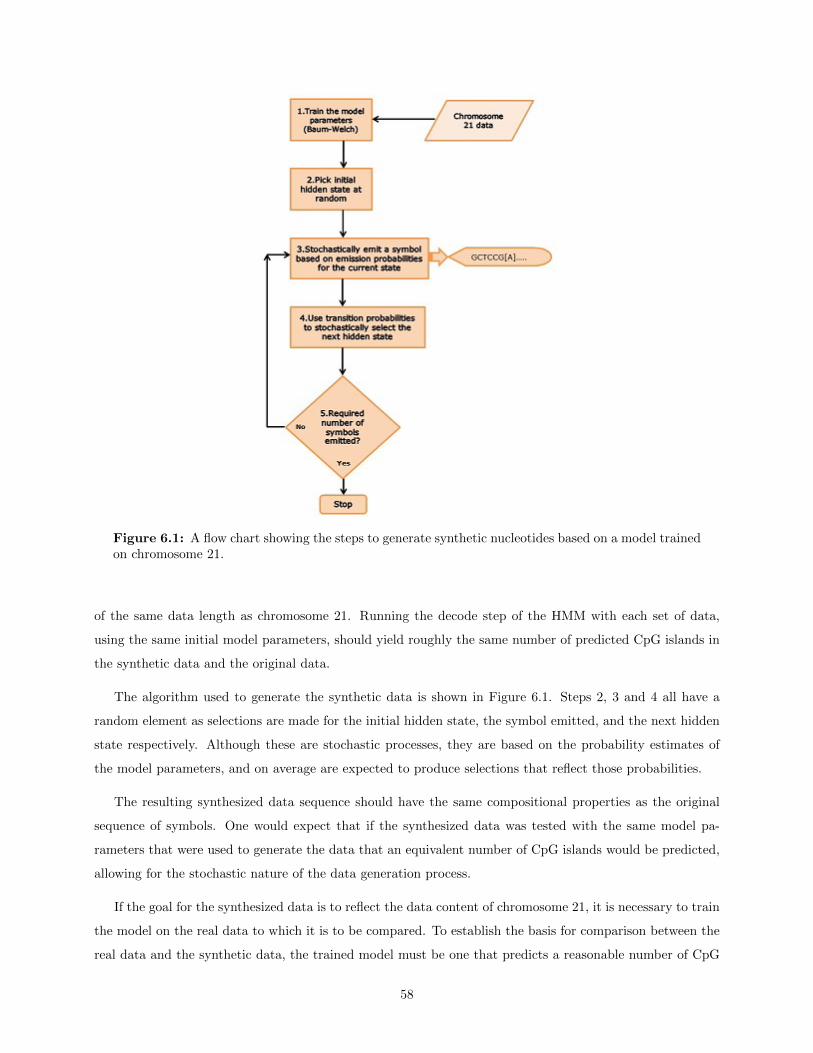
Figure 6.1: A flow chart showing the steps to generate synthetic nucleotides based on a model trainedon chromosome 21.

of the same data length as chromosome 21. Running the decode step of the HMM with each set of data,

using the same initial model parameters, should yield roughly the same number of predicted CpG islands in

the synthetic data and the original data.

The algorithm used to generate the synthetic data is shown in Figure 6.1. Steps 2, 3 and 4 all have a

random element as selections are made for the initial hidden state, the symbol emitted, and the next hidden

state respectively. Although these are stochastic processes, they are based on the probability estimates of

the model parameters, and on average are expected to produce selections that reflect those probabilities.

The resulting synthesized data sequence should have the same compositional properties as the original

sequence of symbols. One would expect that if the synthesized data was tested with the same model pa-

rameters that were used to generate the data that an equivalent number of CpG islands would be predicted,

allowing for the stochastic nature of the data generation process.

If the goal for the synthesized data is to reflect the data content of chromosome 21, it is necessary to train

the model on the real data to which it is to be compared. To establish the basis for comparison between the

real data and the synthetic data, the trained model must be one that predicts a reasonable number of CpG

58

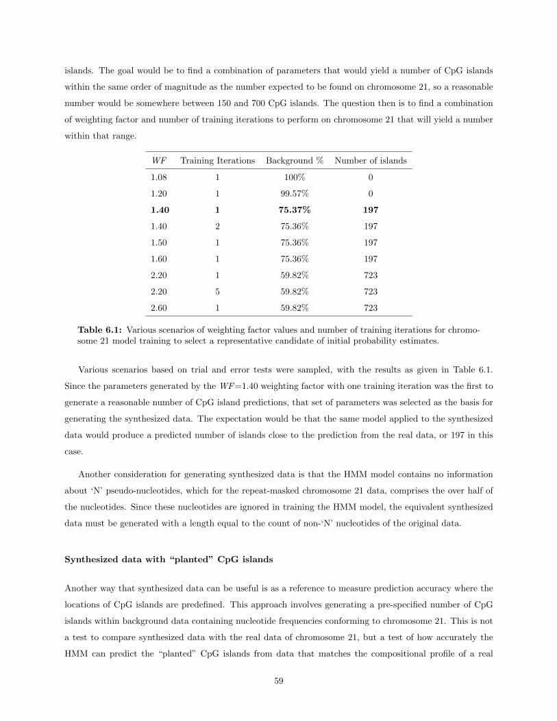
islands. The goal would be to find a combination of parameters that would yield a number of CpG islands

within the same order of magnitude as the number expected to be found on chromosome 21, so a reasonable

number would be somewhere between 150 and 700 CpG islands. The question then is to find a combination

of weighting factor and number of training iterations to perform on chromosome 21 that will yield a number

within that range.

WF Training Iterations Background % Number of islands

1.08 1 100% 0

1.20 1 99.57% 0

1.40 1 75.37% 197

1.40 2 75.36% 197

1.50 1 75.36% 197

1.60 1 75.36% 197

2.20 1 59.82% 723

2.20 5 59.82% 723

2.60 1 59.82% 723

Table 6.1: Various scenarios of weighting factor values and number of training iterations for chromo-some 21 model training to select a representative candidate of initial probability estimates.

Various scenarios based on trial and error tests were sampled, with the results as given in Table 6.1.

Since the parameters generated by the WF=1.40 weighting factor with one training iteration was the first to

generate a reasonable number of CpG island predictions, that set of parameters was selected as the basis for

generating the synthesized data. The expectation would be that the same model applied to the synthesized

data would produce a predicted number of islands close to the prediction from the real data, or 197 in this

case.

Another consideration for generating synthesized data is that the HMM model contains no information

about ‘N’ pseudo-nucleotides, which for the repeat-masked chromosome 21 data, comprises the over half of

the nucleotides. Since these nucleotides are ignored in training the HMM model, the equivalent synthesized

data must be generated with a length equal to the count of non-‘N’ nucleotides of the original data.

Synthesized data with “planted” CpG islands

Another way that synthesized data can be useful is as a reference to measure prediction accuracy where the

locations of CpG islands are predefined. This approach involves generating a pre-specified number of CpG

islands within background data containing nucleotide frequencies conforming to chromosome 21. This is not

a test to compare synthesized data with the real data of chromosome 21, but a test of how accurately the

HMM can predict the “planted” CpG islands from data that matches the compositional profile of a real

59

chromosome, with the advantage that the predictions can be measured against what is known in advance to

be CpG islands, as opposed to the uncertainty associated with the putative connection between CpG islands

and genes.

A specified number of 300 regions that have the characteristics of CpG islands were “planted” in the

synthesized background data. In this test, due to the demonstrated greater accuracy of the second-order

HMM over the first-order HMM, the second-order HMM with model parameters trained against the “extreme”

data (the same second-order HMM used for chromosome 21 predictions) was then run against these data to

predict the number of CpG islands (see Section 5.2.1 on page 47).

To characterize the 300 “planted” regions as CpG islands, the CpG island length, GC content and number

of CpGs expected were profiled by the cumulative frequency curves derived from Figures 5.7, 5.8, and 5.9.

These frequency curves provide the best profile of CpG islands for the synthetic data, assuming that the

CpG islands identified in the second-order HMM test were representative of CpG islands on chromosome 21.

Assuming the CpG islands are representative of chromosome 21, a blanket test similar to what was used with

the second-order HMM (i.e. weighting factors ranging from 0.60 to 0.67 with up to five training iterations)

should yield a highly accurate count of predicted CpG islands in the synthesized data.

6.2 Results

6.2.1 Validation of generated synthetic data

Generation of synthetic data based on HMM model parameters

A first-order HMM model was created based on the repeat-masked chromosome 21 data using a weighting

factor value of 1.40 (see Table 6.1). After a single training iteration, the model generated consisted of

the probabilities shown in Table 6.2. This model predicts 197 CpG islands when run against the original

chromosome 21 data with 75.37% of the hidden states composed of Background states.

The data generation phase used the probabilities given in Table 6.2 to generate data that would be

expected to be compositionally equivalent to the original chromosome 21 data. The data model that had

been trained on the original data was used to decode the sequence of hidden states on the synthesized data.

On completion, the CpGID 2.0 program reported a Background hidden state composition of 73.68%, very

close to the 75.37% reported when run against the original data. The slight decrease in background hidden

states implies a slight increase in Island hidden states, leading to an expectation that the interpretation of

those Island states should result in the same, or more, CpG islands. In spite of the fact that 26.32% of the

hidden states were identified as Island states, the number of predicted CpG islands however, was zero. The

60

WF=1.40 Transition Emission

p(B->B): 0.6893895 p(a|B): 0.360169 p(a|I): 0.2032279

p(B->I): 0.3106104 p(c|B): 0.1401652 p(c|I): 0.2970761

p(I->B): 0.4900271 p(g|B): 0.1400075 p(g|I): 0.2967333

p(I->I): 0.5099729 p(t|B): 0.3596584 p(t|I): 0.2029627

Table 6.2: First-order HMM model parameters trained on chromosome 21 repeat-masked data usingweighting factor value of 1.40. These model parameters predicted a count of 197 CpG islands onchromosome 21 with one training iteration. Each row represents one of the four hidden state transitions,the probability indicated in the Transition column. The Emission column indicates two values for eachrow, representing the probabilities of emitting a particular nucleotide for a given hidden state (forexample, the probability of emitting an ‘A’ given a Background hidden state [B] is 0.360169).

expectation that the synthetic data should generate a similar number of predicted CpG islands was not met.

Generation of synthetic data based on “planted islands” model

The advantage of generating synthesized data based on the idea of “planted CpG islands” is that the exact

location of each CpG island in the DNA sequence is known in advance when running an HMM prediction,

and the accuracy of the prediction can easily be verified. To characterize the CpG islands to be “planted”,

the distribution of properties of the 335 islands predicted by the second-order HMM were used (section 6.1.1,

p. 59). These 335 CpG islands formed the best prediction of CpG islands for the second-order HMM (sec-

tion 5.2.2, p. 48), and their distribution of properties are expressed by the frequency curves in Figures 5.7,

5.8, and 5.9.

Based on these characteristic profiles, a total of 300 CpG islands were generated in a synthetic DNA

sequence of the same length as the unmasked nucleotides of chromosome 21. A series of blanket tests were

then conducted to try to find a combination of weighting factor and number of training iterations that would

predict a number of CpG islands that would be close to 300. A weighting factor ranging from 0.60 to 0.67

with from one to five training iterations proved to yield the desired island counts. The resulting surface graph

is shown in Figure 6.2. The data underlying the surface graph are shown in Table 6.3.

From these data, the 331 CpG islands predicted using weighting factor value 0.60 and 5 training iterations

were selected to determine their predictive accuracy with the 300 CpG islands planted in the synthesized data.

This comparison produced the results described in Table 6.4. The second-order HMM correctly predicted

the location of 84.3% of the planted islands, with a high sensitivity of 93.0%.

Two attempts at generating synthetic DNA data that would model CpG island properties resulted in

two completely opposite results. In the first case, the expectation was that the data generated from the

model parameters derived from real data would accurately reflect the properties of the real data. This test

61

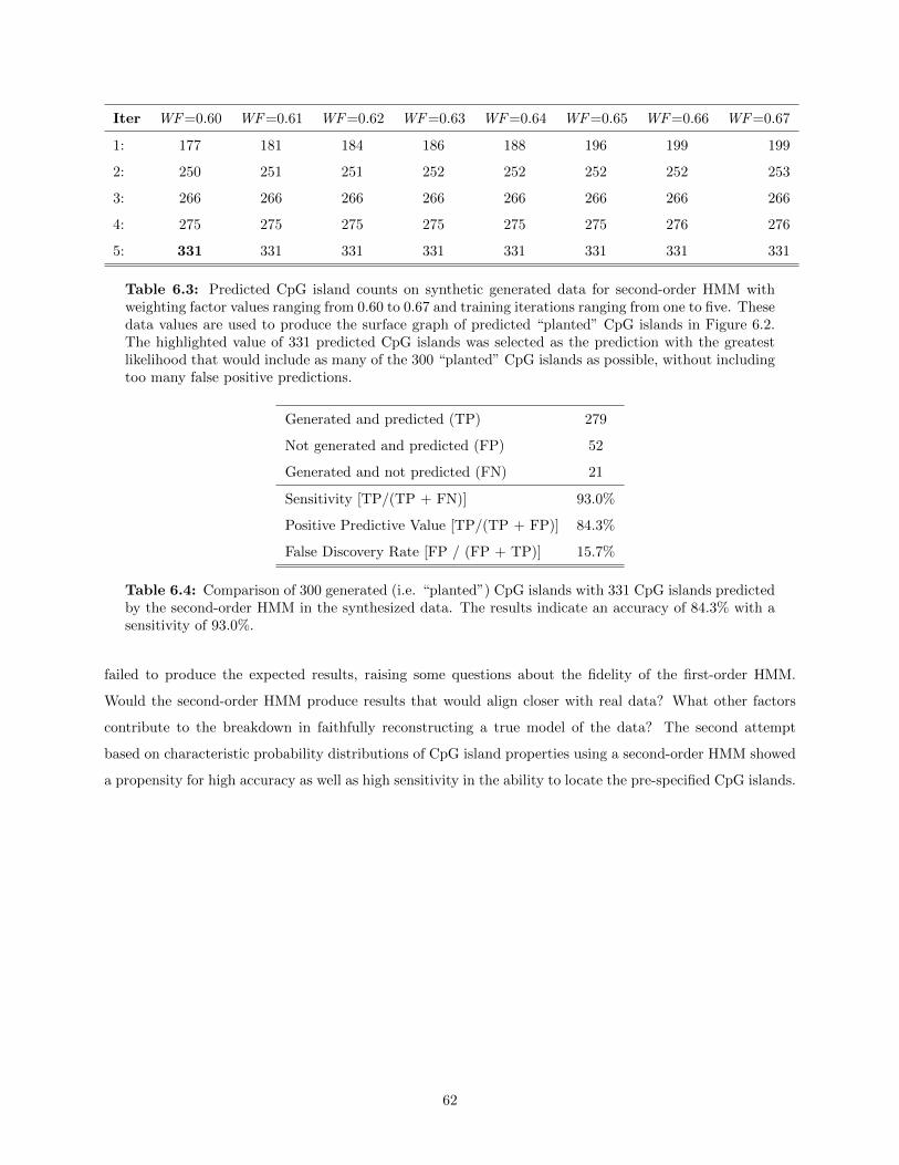
Iter WF=0.60 WF=0.61 WF=0.62 WF=0.63 WF=0.64 WF=0.65 WF=0.66 WF=0.67

1: 177 181 184 186 188 196 199 199

2: 250 251 251 252 252 252 252 253

3: 266 266 266 266 266 266 266 266

4: 275 275 275 275 275 275 276 276

5: 331 331 331 331 331 331 331 331

Table 6.3: Predicted CpG island counts on synthetic generated data for second-order HMM withweighting factor values ranging from 0.60 to 0.67 and training iterations ranging from one to five. Thesedata values are used to produce the surface graph of predicted “planted” CpG islands in Figure 6.2.The highlighted value of 331 predicted CpG islands was selected as the prediction with the greatestlikelihood that would include as many of the 300 “planted” CpG islands as possible, without includingtoo many false positive predictions.

Generated and predicted (TP) 279

Not generated and predicted (FP) 52

Generated and not predicted (FN) 21

Sensitivity [TP/(TP + FN)] 93.0%

Positive Predictive Value [TP/(TP + FP)] 84.3%

False Discovery Rate [FP / (FP + TP)] 15.7%

Table 6.4: Comparison of 300 generated (i.e. “planted”) CpG islands with 331 CpG islands predictedby the second-order HMM in the synthesized data. The results indicate an accuracy of 84.3% with asensitivity of 93.0%.

failed to produce the expected results, raising some questions about the fidelity of the first-order HMM.

Would the second-order HMM produce results that would align closer with real data? What other factors

contribute to the breakdown in faithfully reconstructing a true model of the data? The second attempt

based on characteristic probability distributions of CpG island properties using a second-order HMM showed

a propensity for high accuracy as well as high sensitivity in the ability to locate the pre-specified CpG islands.

62

Figure 6.2: Surface graph illustrating the second-order HMM CpG island predictions of the generatedsynthetic data with “planted” CpG islands.

63

Chapter 7

Comparison with chromosome 22

7.1 Data and Methodology

7.1.1 The chromosome 22 story

Chromosome 22 hg18 data was downloaded and analyzed to provide a basis for comparison between chromo-

some 21 and another data set of comparable data. Chromosome 22, although slightly longer than chromosome

21, contains only 18,111,616 base pairs after masking all repeating and low complexity regions using the same

protocol as with chromosome 21. Surprisingly, instead of the 41% GC average content throughout the human

genome, A, C, G and T content in chromosome 22 are evenly distributed. Table 7.1 provides a comparison

of the content between chromosome 21 and 22. This suggests there might be a larger number of CpG islands

on chromosome 22, along with a correspondingly higher number of genes. Scherf reports on some of the

interesting properties of human chromosome 22, such as the finding that 553 CpG islands were located with

a minimum length of 400 base pairs, a maximum length of 10,000 base pairs and average length of 1074 base

pairs [39].

Base Chr21 Frequency Chr21 Probability Chr22 Frequency Chr22 Probability

A 5475840 0.299 4542742 0.251

C 3678322 0.201 4517675 0.249

G 3674123 0.201 4519275 0.250

T 5468240 0.299 4531924 0.250

Table 7.1: The frequency and probability of each nucleotide in chromosome 21 and 22.

A download of the UCSC hg18 gene list for chromosome 22 did in fact verify that this chromosome

contains 503 genes, an increase from the 273 genes on chromosome 21.

64

7.2 Results

7.2.1 Assessment of human chromosome 22 data

A download of the hg18 CpG islands predicted by the UCSC method revealed 3780 CpG islands on chromo-

some 22, far outnumbering the number of genes present on this chromosome. The Takai and Jones method

was run against the chromosome 22 data following the same protocol as with chromosome 21, with the result

that 610 CpG islands were predicted by this method.

A second-order HMM blanket test was run against human chromosome 22 using the same weighting factor

values and number of training iterations as for chromosome 21. Figure 7.1 shows the resulting surface graph

of the blanket test.

The data underlying the surface graph (Table 7.2) again shows the variability in the number of predicted

CpG islands, particularly with the increase in the number of training iterations. Comparing the predicted

CpG island counts for chromosome 21 in Table 5.11 with those for chromosome 22 in Table 7.2 yields the

expected result that for the same input parameters, roughly twice as many CpG islands are predicted for

chromosome 22.

Iter WF=0.60 WF=0.61 WF=0.62 WF=0.63 WF=0.64 WF=0.65 WF=0.66 WF=0.67

1: 53 80 96 98 106 110 111 121

2: 233 251 260 268 277 294 313 347

3: 379 392 427 453 618 666 796 832

4: 1626 1754 1793 1881 1987 2054 2178 2304

5: 2566 2841 3029 3232 3383 3569 3722 3876

Table 7.2: Data values underlying the outcome of the second-order HMM on chromosome 22 shownin Figure 7.1.

A comparative assessment of chromosome 22 with chromosome 21 appears in Figure 8.1 on page 68,

showing that the difference in data properties of the two chromosomes leads to corresponding differences in

the prediction of CpG islands. Although unintended, the analysis of chromosome 22 provided some assurance

that the HMM methodology performs as expected when the model was trained appropriately.

65

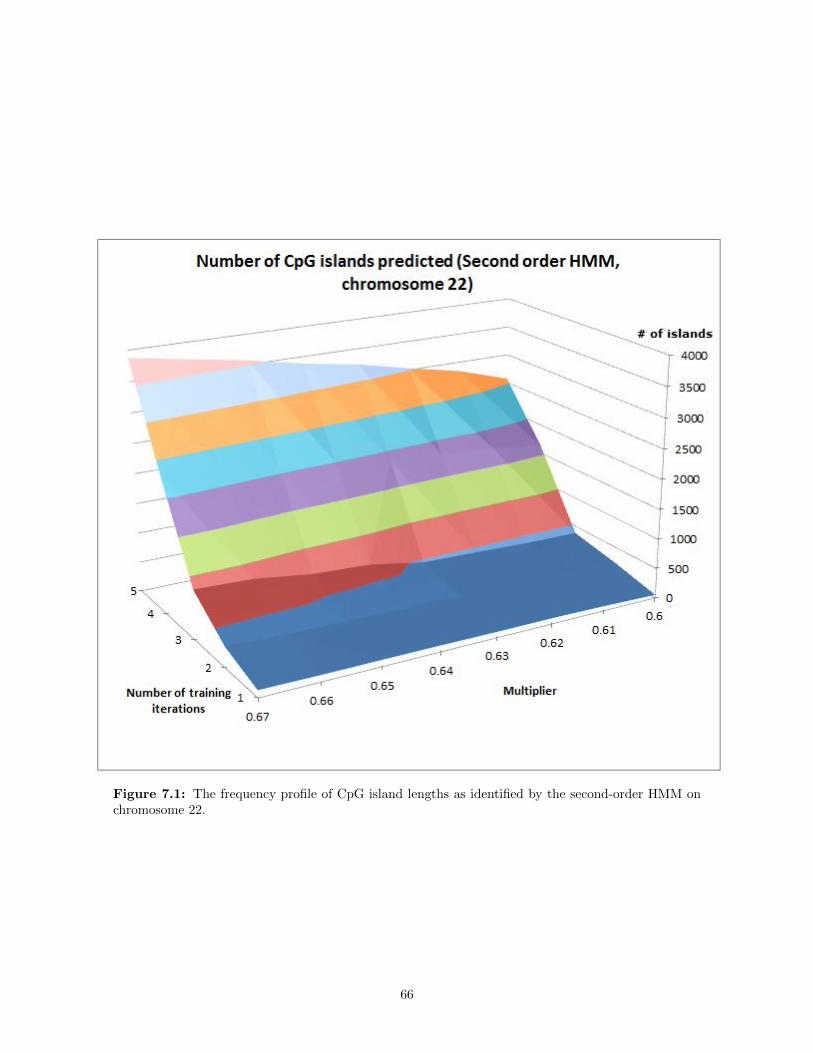
Figure 7.1: The frequency profile of CpG island lengths as identified by the second-order HMM onchromosome 22.

66

Chapter 8

Discussion, Conclusions and Future Work

8.1 Comparison of CpG island predictions for chromosome 21

The improvements to the CpGID 2.0 program enumerated in Section 4.1.4 allowed many consecutive blanket

tests to be run efficiently. For example, running the blanket test that produced the first-order HMM results

of Figure 5.4 on page 49 required an average of 48.4 seconds per prediction, where the test consisted of

predictions for eight different weighting factors and five training iterations for each weighting factor. In this

blanket test, the model parameters were trained on a relatively small set of “extreme” data, and then each

prediction was tested against the complete chromosome 21. In total, this complete blanket test took about

thirty minutes in elapsed time.

A similar blanket test involving six weighting factors and five training iterations for each one took an

average of 48.1 seconds per prediction, and the elapsed time was just over 24 minutes. This blanket test

produced the data reported in Figure 5.6 on page 52.

A recent article describes the implementation of the Baum-Welch algorithm and Viterbi algorithm in an

HMM written in the R programming environment [16]. This implementation is subject to the same memory

and performance limitations as the CpGID 2.0 implementation was, and these limitations could be overcome

somewhat by applying some of the same refactoring techniques as were successful with CpGID 2.0.

8.1.1 Accuracy of CpG island predictions

Applying the HMM theory to various data scenarios and comparing the results with other methods proved

to be illuminating. The primary subject of this thesis was chromosome 21 data, stripped of any content

consisting of low complexity regions. Given the assertion that up to 30% of gene promoters are associated

with CpG islands, the finding that the incidence of CpG islands collocated with gene promoters was in the

range of 5% to 20% for all four methods examined in Table 5.12, while surprising, is partly explained by

the restrictive interpretation of “collocation”. Where the literature tends to include CpG islands anywhere

within or proximal to a gene, this study focused only on the upstream region from the gene transcription

67

start site. Recent reports indicate that when CpG islands within promoter regions are isolated from those

within genes, the CpG islands within promoter regions represent about half of the total [43]. Thus, at most,

the level of collocation in promoter regions could be expected to be about 30%.

Table 5.12 indicates the percentage of gene promoters from chromosome 21 to which each of the four

prediction methods map CpG islands. Although the second-order HMM method fares slightly better than

the first-order HMM method and the Takai and Jones method, they all fall well short of the UCSC CpG

island accuracy. Even the UCSC CpG island map accounts for only about half of the expected number of

CpG islands. Possible explanations are that the prediction methods are not accurate, or chromosome 21 does

not follow the expected pattern of CpG island incidence with promoter regions.

Comparisons of CpG islands predicted by each prediction method

Several observations about the comparison of CpG islands predicted in chromosome 21 by each method led

to interesting conclusions. In spite of the fact that the UCSC method of predicting CpG islands scores higher

than the other three methods, there is very little overlap between the set of islands reported by UCSC and

by all three other methods combined. These two sets are fairly disjointed, with only 10 islands reported in

common (see Section 5.2.2, p. 48).

Table 8.1 gives a complete comparison of the four prediction methods in terms of correct and incorrect

prediction counts, including comparative sensitivity and PPV scores.

Chromosome 21 (273 genes) T&J 1st order HMM 2nd order HMM UCSC

Collocated with gene (TP) 17 20 22 66

Not collocated with genes (FP) 291 339 313 290

Total predicted CpG islands (TP+FP) 308 359 335 356

Genes with no island predicted (FN) 256 253 251 207

Sensitivity [TP/(TP+FN)] 6.2% 7.3% 8.1% 24.2%

PPV [TP/(TP+FP)] 5.5% 5.6% 6.6% 18.5%

FDR (1-PPV) 94.5% 94.4% 93.4% 81.5%

Table 8.1: Summary of measures indicating the quality of first-order HMM predictions of CpG islandsin chromosomes 21 by the various methods. The sensitivity, positive predictive values (PPV) and falsediscovery rate (FDR) allow methods to be compared on a common basis.

Table 8.2 points out a possible explanation for the disjointedness in the predicted island sets. The low

average CG content percentage score and low CpG observed/expected score of the UCSC method suggests

that the different criteria used by this method play a much bigger role than the strict focus on the content

of the DNA sequence alone. In fact, 117 of the CpG islands predicted by the UCSC have no CG content at

all, and 212 of the 356 islands predicted have less than 25% CG content. Characterizing predictions in this

68

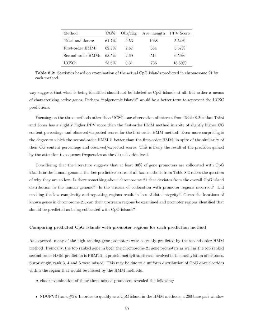
Method CG% Obs/Exp Ave. Length PPV Score

Takai and Jones: 61.7% 2.53 1038 5.54%

First-order HMM: 62.8% 2.67 534 5.57%

Second-order HMM: 63.5% 2.69 514 6.59%

UCSC: 25.6% 0.31 736 18.59%

Table 8.2: Statistics based on examination of the actual CpG islands predicted in chromosome 21 byeach method.

way suggests that what is being identified should not be labeled as CpG islands at all, but rather a means

of characterizing active genes. Perhaps “epigenomic islands” would be a better term to represent the UCSC

predictions.

Focusing on the three methods other than UCSC, one observation of interest from Table 8.2 is that Takai

and Jones has a slightly higher PPV score than the first-order HMM method in spite of slightly higher CG

content percentage and observed/expected scores for the first-order HMM method. Even more surprising is

the degree to which the second-order HMM is better than the first-order HMM, in spite of the similarity of

their CG content percentage and observed/expected scores. This is likely the result of the precision gained

by the attention to sequence frequencies at the di-nucleotide level.

Considering that the literature suggests that at least 30% of gene promoters are collocated with CpG

islands in the human genome, the low predictive scores of all four methods from Table 8.2 raises the question

of why they are so low. Is there something about chromosome 21 that deviates from the overall CpG island

distribution in the human genome? Is the criteria of collocation with promoter regions incorrect? Did

masking the low complexity and repeating regions result in loss of data integrity? Given the locations of

known genes in chromosome 21, can their upstream regions be examined and promoter regions identified that

should be predicted as being collocated with CpG islands?

Comparing predicted CpG islands with promoter regions for each prediction method

As expected, many of the high ranking gene promoters were correctly predicted by the second-order HMM

method. Ironically, the top ranked gene in both the chromosome 21 gene promoters as well as the top ranked

second-order HMM prediction is PRMT2, a protein methyltransferase involved in the methylation of histones.

Surprisingly, rank 3, 4 and 5 were missed. This may be due to a uniform distribution of CpG di-nucleotides

within the region that would be missed by the HMM methods.

A closer examination of these three missed promoters revealed the following:

• NDUFV3 (rank #3): In order to qualify as a CpG island in the HMM methods, a 200 base pair window

69

must have a minimum number of Island hidden states of 70%, or 140 states. In the case of NDUFV3,

the maximum number of Island hidden states in any 200 base pair window within the promoter region

was 136, or 68%.

• ITGB2 (rank #4): The ITGB2 gene promoter had a maximum number of Island hidden states in any

200 base pair window of 123, or 61.5%. The measured promoter region did have a CG content of 3196

base pairs out of 5498 base pairs, or 58%, but not concentrated enough at any one window to qualify

as a CpG island.

• FTCD (rank #5): The FTCD gene promoter had a maximum number of Island hidden states in any

200 base pair window of 137 or 68.5%. There were 2850 CG base pairs out of 5498 base pairs, or 52%.

Due to the uniform distribution of the CG content of the promoter regions of these three genes, they came

close to qualifying as collocated with CpG islands, but narrowly missed out. Lowering the cutoff threshold

from 70% to 61% would have included all three gene promoters collocated with predicted CpG islands, but

would also have resulted in many more CpG islands predicted, possibly suggesting why the number of CpG

islands was under-estimated by the HMM methods. The trade-off involves greater sensitivity at the expense

of less specificity.

In contrast, the second-order HMM predicts a CpG island associated with the RCAN1 gene promoter,

which ranks 181 out of a list of 273 gene promoters. This is explained by the fact that the predicted CpG

island resides just inside the far boundary of the upstream promoter region for RCAN1, and the CpG island

itself has high scoring credentials, while the promoter region as a whole does not. The inclusion of this

promoter may be an artifact of the uniform promoter region size criterion and the generous size assigned to

the putative promoter region upstream from the gene.

On the basis of the ranked list of promoters of chromosome 21, if the cutoff of CpG observed/expected

ratio is set to 0.50 (i.e. an amount about double the expected value for the human genome, but still short

of the 0.65 criterion set by Takai and Jones), 42 gene promoters are identified as putative CpG islands,

or 15% of the 273 genes on chromosome 21, well short of the expected 30% of promoter regions with CpG

islands. The gene promoter region at the 30% ranked level of chromosome 21, KRTAP20-4, has a CG content

percentage of only 25.9% and a CpG observed/expected ratio of 0.11. The average CG content percentage of

all 273 promoter regions is 23.8%, well short of the expected 41% of the human genome average, let alone the

expected elevated CG content in the promoter regions. The promoter regions of chromosome 21 appear to

be CG depleted in relation to the rest of the human genome. This is not true of chromosome 21 as a whole,

as it conforms exactly with the expected 41% CG content of the human genome.

A further possible explanation for the minimal number of true positive predictions is the requirement that

the CpG island be collocated upstream of the gene in the promoter region. Other studies have included CpG

islands in the intragenic region as well as after the end of the gene to be included in the true positive counts.

70

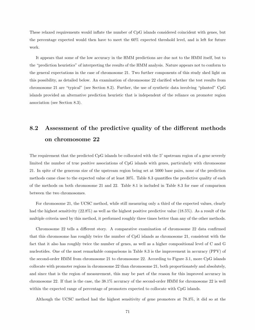
These relaxed requirements would inflate the number of CpG islands considered coincident with genes, but

the percentage expected would then have to meet the 60% expected threshold level, and is left for future

work.

It appears that some of the low accuracy in the HMM predictions are due not to the HMM itself, but to

the “prediction heuristics” of interpreting the results of the HMM analysis. Nature appears not to conform to

the general expectations in the case of chromosome 21. Two further components of this study shed light on

this possibility, as detailed below. An examination of chromosome 22 clarified whether the test results from

chromosome 21 are “typical” (see Section 8.2). Further, the use of synthetic data involving “planted” CpG

islands provided an alternative prediction heuristic that is independent of the reliance on promoter region

association (see Section 8.3).

8.2 Assessment of the predictive quality of the different methods

on chromosome 22

The requirement that the predicted CpG islands be collocated with the 5′ upstream region of a gene severely

limited the number of true positive associations of CpG islands with genes, particularly with chromosome

21. In spite of the generous size of the upstream region being set at 5000 base pairs, none of the prediction

methods came close to the expected value of at least 30%. Table 8.3 quantifies the predictive quality of each

of the methods on both chromosome 21 and 22. Table 8.1 is included in Table 8.3 for ease of comparison

between the two chromosomes.

For chromosome 21, the UCSC method, while still measuring only a third of the expected values, clearly

had the highest sensitivity (22.8%) as well as the highest positive predictive value (18.5%). As a result of the

multiple criteria used by this method, it performed roughly three times better than any of the other methods.

Chromosome 22 tells a different story. A comparative examination of chromosome 22 data confirmed

that this chromosome has roughly twice the number of CpG islands as chromosome 21, consistent with the

fact that it also has roughly twice the number of genes, as well as a higher compositional level of C and G

nucleotides. One of the most remarkable comparisons in Table 8.3 is the improvement in accuracy (PPV) of

the second-order HMM from chromosome 21 to chromosome 22. According to Figure 3.1, more CpG islands

collocate with promoter regions in chromosome 22 than chromosome 21, both proportionately and absolutely,

and since that is the region of measurement, this may be part of the reason for this improved accuracy in

chromosome 22. If that is the case, the 38.1% accuracy of the second-order HMM for chromosome 22 is well

within the expected range of percentage of promoters expected to collocate with CpG islands.

Although the UCSC method had the highest sensitivity of gene promoters at 78.3%, it did so at the

71

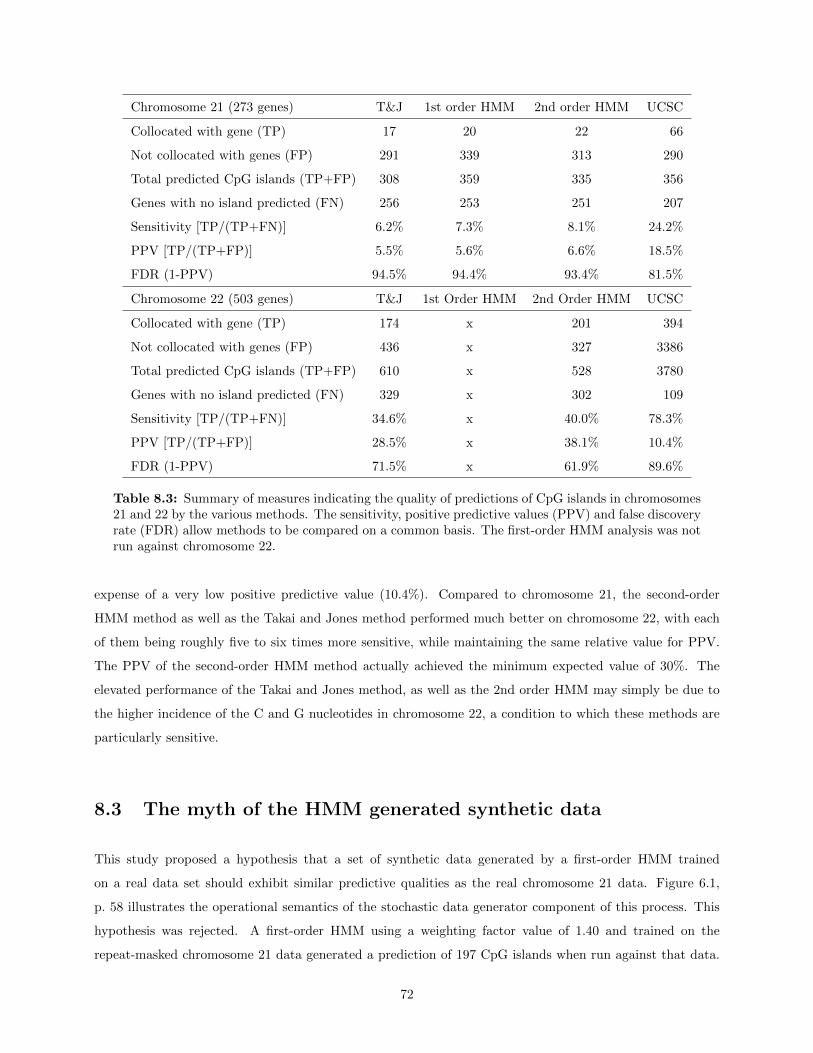
Chromosome 21 (273 genes) T&J 1st order HMM 2nd order HMM UCSC

Collocated with gene (TP) 17 20 22 66

Not collocated with genes (FP) 291 339 313 290

Total predicted CpG islands (TP+FP) 308 359 335 356

Genes with no island predicted (FN) 256 253 251 207

Sensitivity [TP/(TP+FN)] 6.2% 7.3% 8.1% 24.2%

PPV [TP/(TP+FP)] 5.5% 5.6% 6.6% 18.5%

FDR (1-PPV) 94.5% 94.4% 93.4% 81.5%

Chromosome 22 (503 genes) T&J 1st Order HMM 2nd Order HMM UCSC

Collocated with gene (TP) 174 x 201 394

Not collocated with genes (FP) 436 x 327 3386

Total predicted CpG islands (TP+FP) 610 x 528 3780

Genes with no island predicted (FN) 329 x 302 109

Sensitivity [TP/(TP+FN)] 34.6% x 40.0% 78.3%

PPV [TP/(TP+FP)] 28.5% x 38.1% 10.4%

FDR (1-PPV) 71.5% x 61.9% 89.6%

Table 8.3: Summary of measures indicating the quality of predictions of CpG islands in chromosomes21 and 22 by the various methods. The sensitivity, positive predictive values (PPV) and false discoveryrate (FDR) allow methods to be compared on a common basis. The first-order HMM analysis was notrun against chromosome 22.

expense of a very low positive predictive value (10.4%). Compared to chromosome 21, the second-order

HMM method as well as the Takai and Jones method performed much better on chromosome 22, with each

of them being roughly five to six times more sensitive, while maintaining the same relative value for PPV.

The PPV of the second-order HMM method actually achieved the minimum expected value of 30%. The

elevated performance of the Takai and Jones method, as well as the 2nd order HMM may simply be due to

the higher incidence of the C and G nucleotides in chromosome 22, a condition to which these methods are

particularly sensitive.

8.3 The myth of the HMM generated synthetic data

This study proposed a hypothesis that a set of synthetic data generated by a first-order HMM trained

on a real data set should exhibit similar predictive qualities as the real chromosome 21 data. Figure 6.1,

p. 58 illustrates the operational semantics of the stochastic data generator component of this process. This

hypothesis was rejected. A first-order HMM using a weighting factor value of 1.40 and trained on the

repeat-masked chromosome 21 data generated a prediction of 197 CpG islands when run against that data.

72

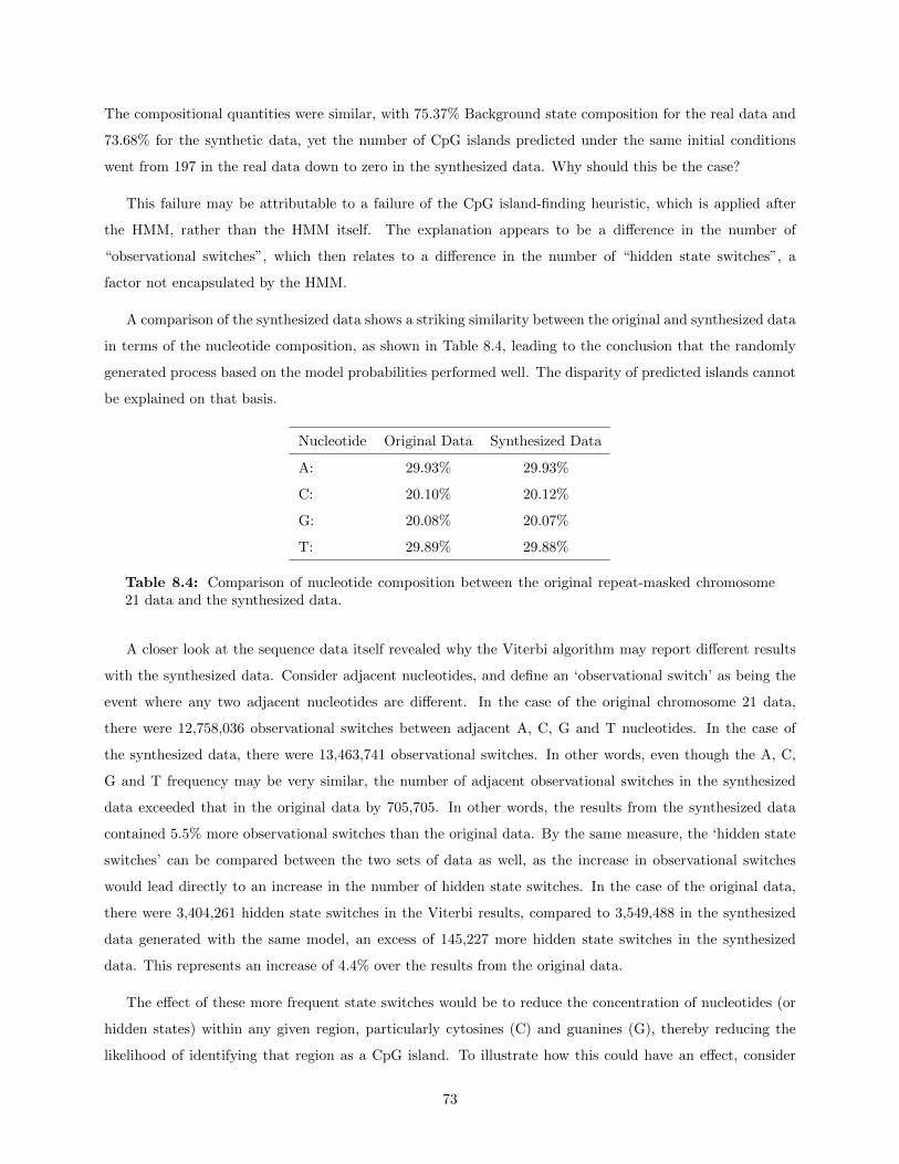
The compositional quantities were similar, with 75.37% Background state composition for the real data and

73.68% for the synthetic data, yet the number of CpG islands predicted under the same initial conditions

went from 197 in the real data down to zero in the synthesized data. Why should this be the case?

This failure may be attributable to a failure of the CpG island-finding heuristic, which is applied after

the HMM, rather than the HMM itself. The explanation appears to be a difference in the number of

“observational switches”, which then relates to a difference in the number of “hidden state switches”, a

factor not encapsulated by the HMM.

A comparison of the synthesized data shows a striking similarity between the original and synthesized data

in terms of the nucleotide composition, as shown in Table 8.4, leading to the conclusion that the randomly

generated process based on the model probabilities performed well. The disparity of predicted islands cannot

be explained on that basis.

Nucleotide Original Data Synthesized Data

A: 29.93% 29.93%

C: 20.10% 20.12%

G: 20.08% 20.07%

T: 29.89% 29.88%

Table 8.4: Comparison of nucleotide composition between the original repeat-masked chromosome21 data and the synthesized data.

A closer look at the sequence data itself revealed why the Viterbi algorithm may report different results

with the synthesized data. Consider adjacent nucleotides, and define an ‘observational switch’ as being the

event where any two adjacent nucleotides are different. In the case of the original chromosome 21 data,

there were 12,758,036 observational switches between adjacent A, C, G and T nucleotides. In the case of

the synthesized data, there were 13,463,741 observational switches. In other words, even though the A, C,

G and T frequency may be very similar, the number of adjacent observational switches in the synthesized

data exceeded that in the original data by 705,705. In other words, the results from the synthesized data

contained 5.5% more observational switches than the original data. By the same measure, the ‘hidden state

switches’ can be compared between the two sets of data as well, as the increase in observational switches

would lead directly to an increase in the number of hidden state switches. In the case of the original data,

there were 3,404,261 hidden state switches in the Viterbi results, compared to 3,549,488 in the synthesized

data generated with the same model, an excess of 145,227 more hidden state switches in the synthesized

data. This represents an increase of 4.4% over the results from the original data.

The effect of these more frequent state switches would be to reduce the concentration of nucleotides (or

hidden states) within any given region, particularly cytosines (C) and guanines (G), thereby reducing the

likelihood of identifying that region as a CpG island. To illustrate how this could have an effect, consider

73

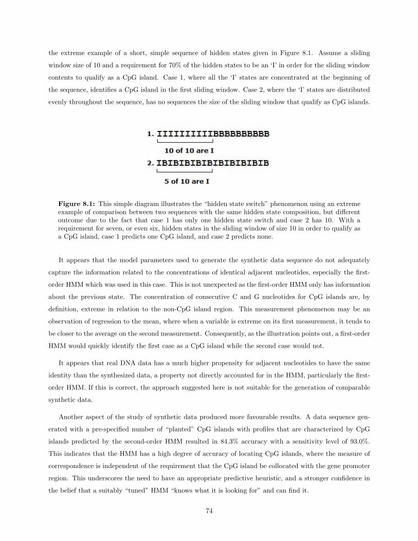
the extreme example of a short, simple sequence of hidden states given in Figure 8.1. Assume a sliding

window size of 10 and a requirement for 70% of the hidden states to be an ‘I’ in order for the sliding window

contents to qualify as a CpG island. Case 1, where all the ‘I’ states are concentrated at the beginning of

the sequence, identifies a CpG island in the first sliding window. Case 2, where the ‘I’ states are distributed

evenly throughout the sequence, has no sequences the size of the sliding window that qualify as CpG islands.

Figure 8.1: This simple diagram illustrates the “hidden state switch” phenomenon using an extremeexample of comparison between two sequences with the same hidden state composition, but differentoutcome due to the fact that case 1 has only one hidden state switch and case 2 has 10. With arequirement for seven, or even six, hidden states in the sliding window of size 10 in order to qualify asa CpG island, case 1 predicts one CpG island, and case 2 predicts none.

It appears that the model parameters used to generate the synthetic data sequence do not adequately

capture the information related to the concentrations of identical adjacent nucleotides, especially the first-

order HMM which was used in this case. This is not unexpected as the first-order HMM only has information

about the previous state. The concentration of consecutive C and G nucleotides for CpG islands are, by

definition, extreme in relation to the non-CpG island region. This measurement phenomenon may be an

observation of regression to the mean, where when a variable is extreme on its first measurement, it tends to

be closer to the average on the second measurement. Consequently, as the illustration points out, a first-order

HMM would quickly identify the first case as a CpG island while the second case would not.

It appears that real DNA data has a much higher propensity for adjacent nucleotides to have the same

identity than the synthesized data, a property not directly accounted for in the HMM, particularly the first-

order HMM. If this is correct, the approach suggested here is not suitable for the generation of comparable

synthetic data.

Another aspect of the study of synthetic data produced more favourable results. A data sequence gen-

erated with a pre-specified number of “planted” CpG islands with profiles that are characterized by CpG

islands predicted by the second-order HMM resulted in 84.3% accuracy with a sensitivity level of 93.0%.

This indicates that the HMM has a high degree of accuracy of locating CpG islands, where the measure of

correspondence is independent of the requirement that the CpG island be collocated with the gene promoter

region. This underscores the need to have an appropriate predictive heuristic, and a stronger confidence in

the belief that a suitably “tuned” HMM “knows what it is looking for” and can find it.

74

8.4 Outcome sensitivity to initial parameter estimates

Figure 5.2 illustrates the sudden increase in the number of predicted CpG islands in human chromosome 21 by

the first-order HMM between weighting factor values of 1.087 and 1.088. In spite of this very small increment

in the weighting factor affecting initial emission probabilities, the jump in islands predicted increased from

about 500 to over 1000. This was not an isolated case, but appeared consistently in both first-order and

second-order HMMs. This is a startling increase for a marginal adjustment in the initial estimates and

indicates that researchers applying HMMs to predictive analyses need to exercise caution and assess where

the tipping points in the data occur for various input values. An interesting challenge would be to determine

how much of this behaviour is due to the heuristic technique for identifying CpG islands from a decoded

state sequence, and how much results from the HMM itself.

This unexpected sensitivity of the HMM algorithm to the initial transition probabilities has been ob-

served by other researchers, who state that “The Baum-Welch algorithm was particularly sensitive. Minute

differences in prior values at times resulted in a drastic overestimates [sic] of CpG islands. This continues to

perplex us, we thought priors were supposed to be weighted less as the training deepened.” [9] Further, Simon

Gordonov states “Interestingly, we found that the re-estimated parameter models had loglikelihoods lower (or

around the same value) than the loglikelihood of the model even before re-estimation from Section 2 that was

used to generate the observed sequence, suggesting that the BW [Baum-Welch] method was sensitive to initial

parameter values.” [16] [emphasis mine] Gordonov attributes the difficulty to “the undesirable convergence of

the algorithm to local maxima, making the identification of model parameters sensitive to initial conditions”.

However, the convergence to local maxima normally occurs following a number of training iterations, an

indication that over-training has occurred. In the current study, the difficulty appears consistently already

within the first re-estimation. This raises an interesting possibility. Perhaps, because of the sheer quantity

of data that is present in a whole chromosome, the model is already over-trained after just one iteration.

Singer et al. mention parameter estimation as an outstanding “technical difficulty” which they “leave as

future work to explore” [40] — again, an acknowledgment of a difficulty but no attempt to resolve it. Our

study suggests that with a high-performance HMM implementation, more scenarios of parameter estimates

can be played out, and parameter estimation becomes more of a careful selection based on the additional

information that the scenarios provide. Only a fortuitous selection of the initial probability estimates after

some careful fine tuning of the initial parameters results in an accurate prediction of the expected number

and distribution of CpG islands.

Both of these references to the sensitivity of the HMM to initial estimates come from unpublished

manuscripts, by authors for whom the remark was an offhand statement peripheral to the subject of their

document, but a significant observation in any case. The mainstream literature appears not to have addressed

this anomalous behaviour of HMMs, let alone even raised an awareness of its existence, possibly due to a

75

reluctance to publish negative results which cannot be easily explained. Perhaps the problem is related to the

amount of data being examined by the HMM, and many HMMs are not applied to bio-molecular sequences as

long as a whole human chromosome. The problem may not be apparent in that context. This unpredictable

behaviour of HMMs may call into question previously published results, and raises the need for caution when

applying HMMs to predictive problems.

8.5 Conclusions

The research effort begun by this thesis has suggested new insight into the behaviour of Hidden Markov Models

under different initial starting conditions. The finding that very slight changes in specific initial probability

estimates can lead to huge differences in outcomes suggests that careful attention to appropriate initial model

parameters is required. While a full explanation of this behaviour awaits further investigation, the realization

of the consequences of unsuitable initial estimates should raise caution with HMM practitioners.

While diagnosing this malady in the HMM behaviour, this thesis also provided an antidote in the form

of a tool that is capable of efficiently and effectively highlighting when the aberrant behaviour occurs, and

making appropriate selection of initial parameters that are most likely to produce the best results (see

Section 4.1.1, p. 25). The performance improvements in the CpGID 2.0 program, both in terms of memory

capacity and processing time, enable a solution space of estimates to be searched quickly. The limitations

and deficiencies of the original CpGID 1.0 program were explored and addressed, resulting in a user-friendly

software component that can be readily applied to many CpG island prediction projects.

As an outgrowth of the development of the CpGID 2.0 modifications, another tool, the TrackMap program,

was created to enhance the analytical capabilities of handling large amounts of genomic and epigenomic data.

The visual experience of collocating genetic and epigenetic elements on multiple simultaneous tracks reinforces

understanding of the functional relationships between those elements. The source code for these software

components is available upon request from the author.

The consistently better accuracy of the implementation of a second-order HMM demonstrates the fea-

sibility of incorporating the additional di-nucleotide contextual information within the HMM parameters.

This thesis also established that this could be accomplished as efficiently as a first-order HMM. One could

speculate on whether there is potential to extend this capability to DNA tri-mers.

What started out as a four-horse race among methods to predict CpG islands in chromosome 21 ended up

with the UCSC method essentially dropping out of the race as not credible in terms of the characteristics of

the CpG islands it was predicting. Of the remaining three, the sliding window with filtering criteria of Takai

and Jones, the CpGID 2.0 first-order HMM and the CpGID 2.0 second-order HMM were comparable, with

the second-order HMM showing leadership in terms of accuracy and sensitivity. One lesson learned is that

76

the “predictive heuristic” used in prediction must be appropriate to what the HMM is modeled to search

for. The requirement for finding association between gene promoter regions in chromosome 21 and predicted

CpG islands produced some unexpectedly low associations. The contrasting conditions of chromosome 22

restored the findings to higher levels of collocation, especially with the second-order HMM.

Although initially unintended, two apparently tangential efforts in this thesis provided additional insight

into the issues raised by the study of the HMM. For example, initially chromosome 22 was selected simply

to provide a comparison to the results of chromosome 21. What the comparison revealed was that the

two chromosomes have dissimilar characteristics that cause chromosome 22 to be much more amenable to

HMM analysis than chromosome 21, assuming that the basis of comparison is the measure of association of

CpG islands and gene promoter regions. Secondly, the experience of generating synthetic data intended to

emulate chromosome 21 provided additional insights. Synthesizing data containing pre-specified “planted”

CpG islands characterized by CpG island probability distributions validated the fact that the HMM is an

effective predictive tool, provided that one measures what the HMM is modeled to find.

Although many researchers of predictive algorithms would consider the Hidden Markov Model story

complete and no longer worthy of further attention, this thesis has raised a warning that HMM results should

not be taken at face value. The disruptive findings summarized above regarding the outcome sensitivity to

initial probability estimates should encourage a fresh look at first finding a rigorous explanation for the

anomalous behaviour, then to find ways to mitigate the cause of the behaviour.

8.6 Future work

At various points throughout previous topics, possible future work has been identified. These points and

several others are highlighted and summarized in this section.

The results of the current study call into question the idea that an HMM will converge on “good” model

parameters with little regard for what the initial parameters are. The study also questions the robustness of

the HMM and its ability to consistently predict the desired content of a data sequence according to the profile

as defined by the initial parameters. Increased number of training iterations on large volumes of data also

lead to rapidly escalating predictions about the predicted number of CpG islands, rather than converging on a

representative sample, suggesting a propensity for rapid over-training. There may be a possibility that a large

volume of data may contribute to over-training even after a single training iteration. Further investigation

is required to provide an explanation of this behaviour.

The extension of the first-order HMM to the second-order HMM using di-nucleotide observations suggests

another novel approach to the ability to incorporate additional information in a set of model parameters.

Instead of, or possibly in addition to, the di-nucleotide observations, the incidence of other observations could

77

be encoded within the model parameters and their combined likelihood evaluated to produce the anticipated

prediction, whether of CpG islands or some other biological feature. Other relevant observation data that

could be measured might include methylation status or nucleosome depletion.

In addition to the challenge of accurately predicting the loci of CpG islands, our study examined the

association of predicted CpG islands and gene promoter regions. As an extension to this task, the relation of

this information to the patterns of gene expression and methylation status of the associated genes is expected

to yield valuable biological information [11], [19], [23], [33], [46], [51]. The synergy resulting from the logical

analysis of the three variables—CpG island locus, methylation status and gene expression pattern—should

yield a wealth of detail about gene regulatory mechanisms, a mechanism of particular pertinence to the

diagnosis, progression and treatment of various pathological conditions.

In addition to this background work, possible future work could carry the results of this study forward

by the following:

• Determine the limit of DNA sequence length, if any, for the current CpGID 2.0 implementation. The

goal would be to be able to handle the longest human chromosomes, thereby enabling a genome-wide

analysis to be run.

• Examine the effects of training the HMM on chromosome 21 and testing on chromosome 22, and vice

versa.

• Given the outcome instability caused by small differences in initial probability estimates, determine how

much of this behaviour is due to the heuristic technique for identifying CpG islands from a decoded

state sequence, and how much might be accounted for by the HMM itself. Is it possible to de-couple

the HMM behaviour from the downstream sliding window heuristic and identify the instability with

either one or the other component?

• Repeat the analysis of chromosome 21 with the second-order HMM, but relax the heuristic threshold

required to recognize a predicted CpG island from 70% to 61%. This setting appears to guarantee

that the promoter regions of all of the top ten genes (by obs/exp ratio) would be included in the

prediction set, as well as possibly many others. The question to be answered is whether this strategy

would introduce too many false positives at a loss of specificity. Apply the same methodology to an

examination of chromosome 22 to see whether the phenomena investigated make chromosome 21 a

special case.

• Repeat the generation of synthetic data based on model parameters with the second-order HMM, with

the hypothesis that the additional information from the second-order allows a benchmark data model

to be generated that conforms better to the real data.

78

• Another fruitful approach to predicting the locations of CpG islands is a class of algorithms known

as distance-based methods, typified by an algorithm described by Hackenberg [17]. Applying this

algorithm to the data examined here would be an interesting comparison to the HMM analysis.

• A recent paper has applied a novel statistical approach to the problem of CpG island prediction and

identification [22], which could assist in addressing the question of de-coupling the behaviour of the

HMM versus the downstream predictive heuristic.

• In addition to the epigenetic effect of methylation status, the work can be extended to consider the link

of gene expression and cancer pathology to histone acetylation and histone methylation, or gene copy

count.

79

References

[1] http://genome.ucsc.edu/cgi-bin/hgTables?command=start. (observed Jan 9, 2012).

[2] Francisco Antequera. Structure, function and evolution of CpG island promoters. Cellular and MolecularLife Sciences, 60(8):1647–58, August 2003.

[3] John A. D. Aston and Donald E. K. Martin. Distributions associated with general runs and patterns inhidden Markov models. Annals of Applied Statistics, 1(2):585–611, December 2007.

[4] Adrian Bird. DNA methylation patterns and epigenetic memory. Genes & development, 16(1):6–21,January 2002.

[5] Adrian P. Bird. CpG islands as gene markers in the vertebrate nucleus. Trends in Genetics, 3:342–347,1987.

[6] Christoph Bock, Jorn Walter, Martina Paulsen, and Thomas Lengauer. CpG island mapping byepigenome prediction. PLoS Computational Biology, 3(6):1055–1070, June 2007.

[7] Wai Ki Ching, Eric S. Fung, and Michael K. Ng. Higher-order Markov chain models for categorical datasequences. Naval Research Logistics, 51(4):557–574, June 2004.

[8] Gary A Churchill. Stochastic models for heterogeneous DNA sequence. Bulletin of Mathematical Biology,51(1):79–94, 1989.

[9] Nathan Clement, Dave Elzinga, and Alina Schmidt. Hidden Markov Models and Unsupervised TrainingWith Respect to CpG Islands of Prokaryote and Eukaryote Genomes. psoda4.cs.byu.edu/~nclement/Lab_Report_2.pdf, 2007. [Unpublished manuscript; accessed March 11, 2013].

[10] Richard Durbin, Steve Eddy, Anders Krogh, and Graeme Mitchison. Biological Sequence Analysis:Probabilistic models of proteins and nucleic acids. Cambridge University Press, 1998.

[11] ShiCai Fan, JianXiao Zou, HongBing Xu, and XueGong Zhang. Predicted methylation landscape of allCpG islands on the human genome. Chinese Science Bulletin, 55(22):2353–2358, August 2010.

[12] Robert D Finn, Jody Clements, and Sean R Eddy. HMMER web server: interactive sequence similaritysearching. Nucleic Acids Research, 39:W29–37, July 2011.

[13] Paul Flicek, M Ridwan Amode, Daniel Barrell, Kathryn Beal, Simon Brent, Yuan Chen, Peter Clapham,Guy Coates, Susan Fairley, Stephen Fitzgerald, Leo Gordon, Maurice Hendrix, Thibaut Hourlier, NathanJohnson, Andreas Kahari, Damian Keefe, Stephen Keenan, Rhoda Kinsella, Felix Kokocinski, Eu-gene Kulesha, Pontus Larsson, Ian Longden, William McLaren, Bert Overduin, Bethan Pritchard,Harpreet Singh Riat, Daniel Rios, Graham R S Ritchie, Magali Ruffier, Michael Schuster, Daniel Sobral,Giulietta Spudich, Y Amy Tang, Stephen Trevanion, Jana Vandrovcova, Albert J Vilella, Simon White,Steven P Wilder, Amonida Zadissa, Jorge Zamora, Bronwen L Aken, Ewan Birney, Fiona Cunningham,Ian Dunham, Richard Durbin, Xose M Fernandez-Suarez, Javier Herrero, Tim J P Hubbard, AnneParker, Glenn Proctor, Jan Vogel, and Stephen M J Searle. Ensembl 2011. Nucleic acids research,39(Database issue):D800–6, January 2011.

[14] Katheleen Gardiner and Muriel Davisson. The sequence of human chromosome 21 and implications forresearch into Down syndrome. Genome Biology, 1(2):1–9, 2000.

80

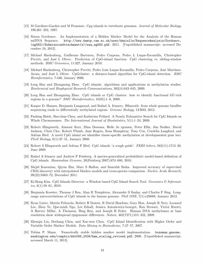
[15] M Gardiner-Garden and M Frommer. Cpg islands in vertebrate genomes. Journal of Molecular Biology,196:261–282, 1987.

[16] Simon Gordonov. An Implementation of a Hidden Markov Model for the Analysis of the HumanmtDNA Sequence. http://www.damtp.cam.ac.uk/user/danielle/SequenceAnalysis/Gordonov,

(sg582)/SubmissionAttachment(s)/saa_sg582.pdf, 2011. [Unpublished manuscript; accessed De-cember 10, 2012].

[17] Michael Hackenberg, Guillermo Barturen, Pedro Carpena, Pedro L Luque-Escamilla, ChristopherPreviti, and Jose L Oliver. Prediction of CpG-island function: CpG clustering vs. sliding-windowmethods. BMC Genomics, 11:327, January 2010.

[18] Michael Hackenberg, Christopher Previti, Pedro Luis Luque-Escamilla, Pedro Carpena, Jose Martınez-Aroza, and Jose L Oliver. CpGcluster: a distance-based algorithm for CpG-island detection. BMCBioinformatics, 7:446, January 2006.

[19] Leng Han and Zhongming Zhao. CpG islands: algorithms and applications in methylation studies.Biochemical and Biophysical Research Communications, 382(4):643–645, 2009.

[20] Leng Han and Zhongming Zhao. CpG islands or CpG clusters: how to identify functional GC-richregions in a genome? BMC Bioinformatics, 10(65):1–6, 2009.

[21] Kasper D. Hansen, Benjamin Langmead, and Rafael A. Irizarry. BSmooth: from whole genome bisulfitesequencing reads to differentially methylated regions. Genome Biology, 13:R83, 2012.

[22] Fushing Hsieh, Shu-chun Chen, and Katherine Pollard. A Nearly Exhaustive Search for CpG Islands onWhole Chromosomes. The International Journal of Biostatistics, 5(1):1–24, 2009.

[23] Robert Illingworth, Alastair Kerr, Dina Desousa, Helle Jø rgensen, Peter Ellis, Jim Stalker, DavidJackson, Chris Clee, Robert Plumb, Jane Rogers, Sean Humphray, Tony Cox, Cordelia Langford, andAdrian Bird. A novel CpG island set identifies tissue-specific methylation at developmental gene loci.PLoS Biology, 6(1):37–51, January 2008.

[24] Robert S Illingworth and Adrian P Bird. CpG islands–’a rough guide’. FEBS letters, 583(11):1713–20,June 2009.

[25] Rafael A Irizarry and Andrew P Feinberg. A species-generalized probabilistic model-based definition ofCpG islands. Mammalian Genome, 20(Feinberg 2007):674–680, 2010.

[26] Majid Kazemian, Qiyun Zhu, Marc S Halfon, and Saurabh Sinha. Improved accuracy of supervisedCRM discovery with interpolated Markov models and cross-species comparison. Nucleic Acids Research,39(22):9463–72, December 2011.

[27] Ki-Bong Kim. CpG Islands Detector: a Window-based CpG Island Search Tool. Genomics & Informat-ics, 8(1):58–61, 2010.

[28] Benjamin Koester, Thomas J Rea, Alan R Templeton, Alexander S Szalay, and Charles F Sing. Long-range autocorrelations of CpG islands in the human genome. PloS ONE, 7(1):e29889, January 2012.

[29] Ryan Lister, Mattia Pelizzola, Robert H Dowen, R David Hawkins, Gary Hon, Joseph R Nery, LeonardLee, Zhen Ye, Que-minh Ngo, Lee Edsall, Jessica Antosiewicz-bourget, Ron Stewart, Victor Ruotti,A Harvey Millar, A Thomson, Bing Ren, and Joseph R Ecker. Human DNA methylomes at baseresolution show widespread epigenomic differences. Nature, 462(7271):315–322, 2009.

[30] Zhenqiu Liu, Dechang Chen, and Xue-wen Chen. CpG Island Identification with Higher Order andVariable Order Markov Models. Data Mining in Biomedicine, 7:47–57, 2007.

[31] Tobias P. Mann. Numerically stable hidden markov model implementation. bozeman.genome.

washington.edu/compbio/mbt599_2006/hmm_scaling_revised.pdf, 2006. [Unpublished manuscript;accessed March 11, 2013].

81

[32] Beatson Institute of Cancer Research. http://www.beatson.gla.ac.uk/. Beatson Institute of CancerResearch.

[33] Christopher Previti, Oscar Harari, Igor Zwir, and Coral del Val. Profile analysis and prediction oftissue-specific CpG island methylation classes. BMC Bioinformatics, 10:116, January 2009.

[34] Lawrence R. Rabiner. A tutorial on hidden Markov models and selected applications in speech recogni-tion. Proceedings of the IEEE, 77(2):257–286, 1989.

[35] Peter N Robinson, Ulrike Bohme, Rodrigo Lopez, Stefan Mundlos, and Peter Nurnberg. Gene-Ontologyanalysis reveals association of tissue-specific 5’ CpG-island genes with development and embryogenesis.Human Molecular Genetics, 13(17):1969–78, September 2004.

[36] Stephen L. Salzberg, Mihaela Pertea, Arthur L. Delcher, Malcom J. Gardner, and Herve Tettelin. In-terpolated Markov models for eukaryotic gene finding. Genomics, 59(1):24–31, July 1999.

[37] Serge Saxonov, Paul Berg, and Douglas L Brutlag. A genome-wide analysis of CpG dinucleotides in thehuman genome distinguishes two distinct classes of promoters. Proceedings of the National Academy ofSciences of the United States of America, 103(5):1412–7, January 2006.

[38] E Scarano, M Iaccarino, P Grippo, and E Parisi. The heterogeneity of thymine methyl group origin inDNA pyrimidine isostichs of developing sea urchin embryos. Proceedings of the National Academy ofSciences of the USA, 57(5):1394–1400, 1967.

[39] Matthias Scherf, Andreas Klingenhoff, Kornelie Frech, Kerstin Quandt, Ralf Schneider, Korbinian Grote,Matthias Frisch, Alexander Seidel, Ruth Brack-werner, and Thomas Werner. First Pass Annotation ofPromoters on Human Chromosome 22. Genome Research, 11(3):333–340, 2001.

[40] Meromit Singer and Alexander Engstr. Determining coding CpG islands by identifying regions significantfor pattern statistics on Markov chains. Statistical Applications in Genetics and Molecular Biology,10(1):1–27, 2011.

[41] Hubley R Smit, AFA and P. Green. http://www.repeatmasker.org. RepeatMasker Open-3.0. 1996-2010.

[42] Leah Spontaneo and Nick Cercone. Correlating CpG islands, motifs, and sequence variants in humanchromosome 21. BMC Genomics, 12 Suppl 2(Suppl 2):S10, January 2011.

[43] Jianzhong Su, Yan Zhang, Jie Lv, Hongbo Liu, Xiaoyan Tang, Fang Wang, Yunfeng Qi, Yujia Feng,and Xia Li. CpG MI: a novel approach for identifying functional CpG islands in mammalian genomes.Nucleic Acids Research, 38(1):1–11, January 2010.

[44] Daiya Takai and Peter Jones. Comprehensive analysis of CpG islands in human chromosomes 21 and 22.Proceedings of the National Academy of Sciences of the United States of America, 99(6):3740–5, March2002.

[45] Yong Wang and Frederick C C Leung. An evaluation of new criteria for CpG islands in the humangenome as gene markers. Bioinformatics, 20(7):1170–7, May 2004.

[46] Hao Wu, Brian Caffo, Harris a Jaffee, Rafael a Irizarry, and Andrew P Feinberg. Redefining CpG islandsusing hidden Markov models. Biostatistics, 11(3):499–514, July 2010.

[47] X Y Xie, X Sun, J M Xie, and Z H Lu. An interpolated Markov model polishes Gibbs sampling’sability in detecting regulatory elements. Proceedings of the Annual International Conference of theIEEE Engineering in Medicine and Biology Society, 4:2801–4, January 2004.

[48] Han Xu, Chia-Lin Wei, Feng Lin, and Wing-Kin Sung. An HMM approach to genome-wide identificationof differential histone modification sites from ChIP-seq data. Bioinformatics, 24(20):2344–9, October2008.

82

[49] Yoichi Yamada, Hidemi Watanabe, Fumihito Miura, Hidenobu Soejima, Michiko Uchiyama, TsuyoshiIwasaka, Tsunehiro Mukai, Yoshiyuki Sakaki, and Takashi Ito. A Comprehensive Analysis of AllelicMethylation Status of CpG Islands on Human Chromosome 21q. Genome Research, 14(2):247–266,2004.

[50] Sujuan Ye, Asai Asaithambi, and Yunkai Liu. CpGIF : an algorithm for the identification of CpG islands.Bioinformation, 2(8):335–338, 2008.

[51] Yingying Zhang, Christian Rohde, Sascha Tierling, Tomasz P Jurkowski, Christoph Bock, Diana San-tacruz, Sergey Ragozin, Richard Reinhardt, Marco Groth, Jorn Walter, and Albert Jeltsch. DNAmethylation analysis of chromosome 21 gene promoters at single base pair and single allele resolution.PLoS Genetics, 5(3):1–15, March 2009.

83

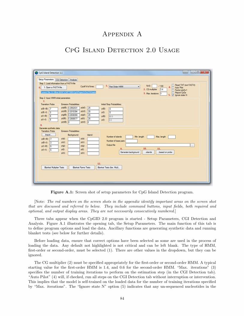
Appendix A

CpG Island Detection 2.0 Usage

Figure A.1: Screen shot of setup parameters for CpG Island Detection program.

[Note: The red numbers on the screen shots in the appendix identify important areas on the screen shotthat are discussed and referred to below. They include command buttons, input fields, both required andoptional, and output display areas. They are not necessarily consecutively numbered.]

Three tabs appear when the CpGID 2.0 program is started - Setup Parameters, CGI Detection andAnalysis. Figure A.1 illustrates the opening tab, the Setup Parameters. The main function of this tab isto define program options and load the data. Ancillary functions are generating synthetic data and runningblanket tests (see below for further details).

Before loading data, ensure that correct options have been selected as some are used in the process ofloading the data. Any default not highlighted is not critical and can be left blank. The type of HMM,first-order or second-order, must be selected (1). There are other values in the dropdown, but they can beignored.

The CG multiplier (2) must be specified appropriately for the first-order or second-order HMM. A typicalstarting value for the first-order HMM is 1.4, and 0.6 for the second-order HMM. “Max. iterations” (3)specifies the number of training iterations to perform on the estimation step (in the CGI Detection tab).“Auto Pilot” (4) will, if checked, run all steps on the CGI Detection tab without interruption or intervention.This implies that the model is self-trained on the loaded data for the number of training iterations specifiedby “Max. iterations”. The “Ignore state N” option (5) indicates that any un-sequenced nucleotides in the

84

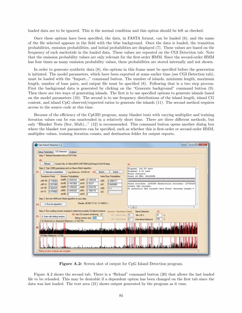
loaded data are to be ignored. This is the normal condition and this option should be left as checked.

Once these options have been specified, the data, in FASTA format, can be loaded (6), and the nameof the file selected appears in the field with the blue background. Once the data is loaded, the transitionprobabilities, emission probabilities, and initial probabilities are displayed (7). These values are based on thefrequency of each nucleotide in the loaded data. These values are repeated on the CGI Detection tab. Notethat the emission probability values are only relevant for the first-order HMM. Since the second-order HMMhas four times as many emission probability values, these probabilities are stored internally and not shown.

In order to generate synthetic data (8), the options in this frame must be specified before the generationis initiated. The model parameters, which have been exported at some earlier time (see CGI Detection tab),must be loaded with the “Import...” command button. The number of islands, minimum length, maximumlength, number of base pairs, and output file must be specified (8). Following that is a two step process.First the background data is generated by clicking on the “Generate background” command button (9).Then there are two ways of generating islands. The first is to use specified options to generate islands basedon the model parameters (10). The second is to use frequency distributions of the island length, island CGcontent, and island CpG observed/expected ratios to generate the islands (11). The second method requiresaccess to the source code at this time.

Because of the efficiency of the CpGID program, many blanket tests with varying multiplier and trainingiteration values can be run unattended in a relatively short time. There are three different methods, butonly “Blanket Tests (Iter, Mult)...” (12) is recommended. This command button opens another dialog boxwhere the blanket test parameters can be specified, such as whether this is first-order or second-order HMM,multiplier values, training iteration counts, and destination folder for output reports.

Figure A.2: Screen shot of output for CpG Island Detection program.

Figure A.2 shows the second tab. There is a “Reload” command button (20) that allows the last loadedfile to be reloaded. This may be desirable if a dependent option has been changed on the first tab since thedata was last loaded. The text area (21) shows output generated by the program as it runs.

85

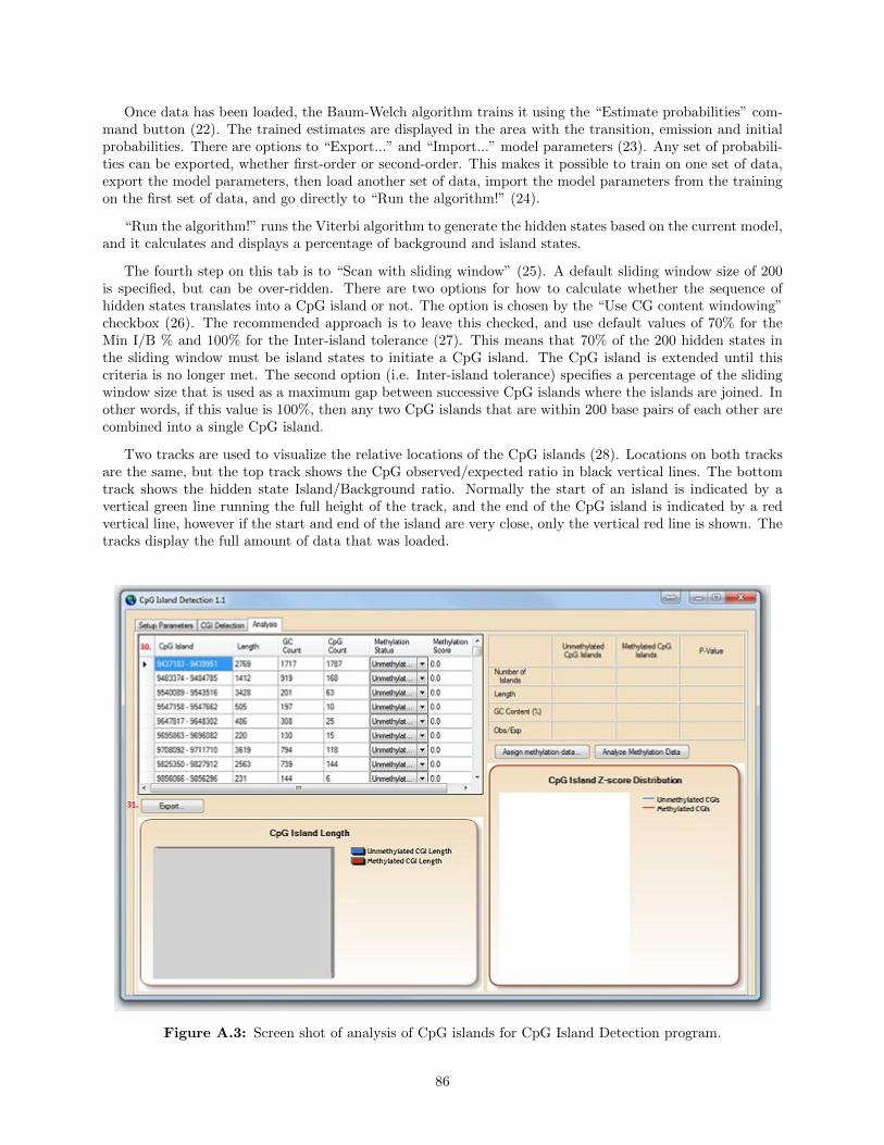
Once data has been loaded, the Baum-Welch algorithm trains it using the “Estimate probabilities” com-mand button (22). The trained estimates are displayed in the area with the transition, emission and initialprobabilities. There are options to “Export...” and “Import...” model parameters (23). Any set of probabili-ties can be exported, whether first-order or second-order. This makes it possible to train on one set of data,export the model parameters, then load another set of data, import the model parameters from the trainingon the first set of data, and go directly to “Run the algorithm!” (24).

“Run the algorithm!” runs the Viterbi algorithm to generate the hidden states based on the current model,and it calculates and displays a percentage of background and island states.

The fourth step on this tab is to “Scan with sliding window” (25). A default sliding window size of 200is specified, but can be over-ridden. There are two options for how to calculate whether the sequence ofhidden states translates into a CpG island or not. The option is chosen by the “Use CG content windowing”checkbox (26). The recommended approach is to leave this checked, and use default values of 70% for theMin I/B % and 100% for the Inter-island tolerance (27). This means that 70% of the 200 hidden states inthe sliding window must be island states to initiate a CpG island. The CpG island is extended until thiscriteria is no longer met. The second option (i.e. Inter-island tolerance) specifies a percentage of the slidingwindow size that is used as a maximum gap between successive CpG islands where the islands are joined. Inother words, if this value is 100%, then any two CpG islands that are within 200 base pairs of each other arecombined into a single CpG island.

Two tracks are used to visualize the relative locations of the CpG islands (28). Locations on both tracksare the same, but the top track shows the CpG observed/expected ratio in black vertical lines. The bottomtrack shows the hidden state Island/Background ratio. Normally the start of an island is indicated by avertical green line running the full height of the track, and the end of the CpG island is indicated by a redvertical line, however if the start and end of the island are very close, only the vertical red line is shown. Thetracks display the full amount of data that was loaded.

Figure A.3: Screen shot of analysis of CpG islands for CpG Island Detection program.

86

Figure A.3 shows the third tab of the program, the Analysis tab. The grid (30) lists the CpG islandsidentified in the tracks on the previous tab resulting from running the sliding window scan. The list ofCpG islands, with there addresses, CG content and observed/expected values, can be exported with the“Export...” command button (31) on this tab. The data is exported as a tab-delimited data file that can beimported into Excel for further analysis.

Other information on this tab is intended for further methylation status analysis, but this has not beenfully developed and can be ignored.

87