Exploring Life through Logic Programming:Logic Programming in Bioinformatics

Alessandro Dal Palu1, Agostino Dovier2,Andrea Formisano3, and Enrico Pontelli4

1 University of Parma, Dip. di Matematica2 University of Udine, Dip. di Matematica e Informatica

3 University of Perugia, Dip. di Matematica e Informatica4 New Mexico State University, Dept. of Computer Science

Abstract. This chapter provides a broad overview of how logic pro-gramming, and in particular Answer Set Programming, can be used tomodel and solve some popular and challenging classes of problems in thegeneral domain of bionformatics. In particular, the chapter explores theuse of ASP in Genomics studies, such as Haplotype inference and Phy-logenetic inference, in Structural studies, such as RNA secondary struc-ture prediction and Protein structure prediction, and in Systems Biology.The chapter offers a brief introduction to biology and bioinformatics andworking ASP code fragments for the various problems investigated.

1 Introduction

Recent advances in the field of Biology have uniquely built on the use of com-putational methods to model, simulate, and sift through dauntingly large datarepositories. The synergistic interaction with biologists and other scientists inthe life sciences has provided computer scientists with a broad range of challeng-ing problems. Problems are often hidden or vaguely specified, and emerge onlyafter long discussions with biologists, physicists, chemistry researchers, medicalclinicians, etc. The effective resolution of these problems has the potential ofhaving a profound impact on our ability to understand the basic mechanismsof life and to advance medical research. Bioinformatics can be broadly definedas the area of Computer Science that deals with modeling and solving problemsfrom biology and related life sciences.

In very broad strokes, we can classify typical bioinformatics application do-mains in three general categories. The first class includes applications of compu-tational methods as a support infrastructure for analysis and experiments; this isthe case, for example, of automated environments for workflow management, de-scription and annotation of experiments, minimal reporting requirements (e.g.,MIAME), etc. The second class includes problems that are efficiently solvable(e.g., in polynomial time), but commonly applied to very large data sets (e.g.,BLAST searches and other string matching problems [98, 67, 63]). Finally, thethird class includes problems that are intractable (i.e., NP-complete or worse),

even under simplifying assumptions; this is the case, for example, of problems re-lated to ab-initio protein structure prediction and to synthesis of gene regulatorynetworks.

Bioinformatics problems can also be classified according to the target of thestudy. Genomics studies focus on the investigation of genomes; genomic studiesoften rely on tractable algorithms applied to very large amounts of data, such asDNA and RNA sequences. Structural studies focus on the prediction and recog-nition of the spatial structure of biomolecules (e.g., proteins); problems in thisclass are often intractable and based on data sets that are relatively smaller thanthose used in genomic studies. Systems studies (a.k.a. systems biology) investi-gate the complex interactions among components (e.g., genes) of a biologicalsystem; these studies typically belong to high complexity classes. The interestedreader can refer to [23, 81, 117] for an introduction to computational biology.

The literature has highlighted the potential for logic programming technologyto address problems in all of these areas (see, e.g. [5]). Prolog and other logic pro-gramming paradigms have been employed in supporting workflow management—e.g., data formats interoperation, service composition (e.g., [91])—and queryingtasks—e.g., querying phylogenetic databases [21]. Nevertheless, the capabilitiesof logic programming—especially Constraint Logic Programming (CLP) and An-swer Set Programming (ASP)—to tackle complex combinatorial problems makethis paradigm particularly appealing to address problems in the third class. Logicprogramming offers some distinct advantages; in particular:

– Models are rarely stable and static—logic programming provides the level ofelaboration-tolerance to support model modifications and incremental addi-tion of new knowledge.

– The use of more traditional techniques, such as linear programming, is ofteninadequate (e.g., incapable of capturing the complexity of realistic energymodels).

In this manuscript, we will provide a broad overview of how ASP can be used tomodel and solve some popular and challenging classes of Bioinformatics prob-lems. In particular, we will explore ASP in

– Genomics studies: we will investigate problems associated to Haplotype in-ference and Phylogenetic inference;

– Structural studies: we will investigate problems associated to RNA secondarystructure prediction and Protein structure prediction;

– Systems studies: we will investigate problems associated to reasoning withbiological networks.

The manuscript represents a coherent synthesis of previous research contribu-tions (as found in the literature, including some the authors’ own work) as wellas novel problem formalizations. The content of this paper also builds on our do-main knowledge gained by organizing the Workshop on Constraint-based Meth-ods in Bioinformatics yearly from 2005 (see, e.g., cp2013.a4cp.org/workshops/wcb), and related publications (e.g., [31, 36, 1]).

2 Biology in a nutshell

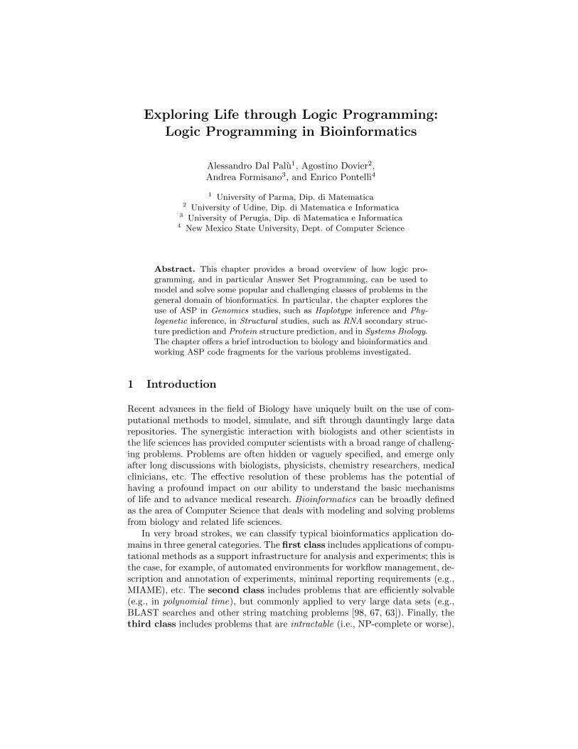
The well known central dogma of Biology was first introduced in 1958 by F.Crick [30] and describes how the biologically relevant information migrates fromDNA sequences to RNA sequences and finally to proteins, whose function isdetermined by their 3D structure. The conversion DNA ↪→ RNA is called tran-scription, while the conversion RNA ↪→ Protein is called translation. Let usbriefly review the above notions in order to understand the central dogma.

DNA (DeoxyriboNucleic Acid) is characterized by a sequence of nucleotidesof 4 kinds: A, C, G, and T (Adenine, Cytosine, Guanine, Thymine). The nu-cleotides have a different atomic composition, omitted here; however they sharea common substructure, that is used to connect sequences of nucleotides intopolymeric strands of potentially unlimited length. Typically, DNA strands havea high propensity to pair: two strands can be aligned and facing nucleotides,one from each strand, can form a relatively stable binding. Some nucleotidematchings are more favorable than others; in particular, there is a notion ofcomplementary string. Precisely, given a sequence s ∈ {A,C,G, T}∗, its comple-mentary sequence s is obtained by reversing the sequence order and by substitut-ing A↔ T and C ↔ G. A string s and its complementary string s form bindingsbetween each pair of corresponding nucleotides, and together they fold into thefamous double helix (see, e.g., the DNA strands at both sides of Figure 1).

TC

GC

G A T C GG

A

T

A G C G C U A G C C U AmRNA

DNA

S A S L Protein

transcription

translation

A

GC

GC T A G

CC

TA

Fig. 1. Schematic view of the central dogma: DNA double helix, transcription to RNAand translation to Protein.

Observed DNA strings are huge (106–1010 nucleotides). Differences betweenthe DNAs of two members of the same specie are limited (e.g., 1 in 1,000 nu-cleotides for humans). Some fragments of the DNA encode proteins, as we showbelow. These regions encode information as described by the central dogma andthey are called genes. Other regions perform other tasks that are beyond the

focus of this manuscript. With the inception of the Human Genome Project,1 itbecame possible to estimate that the human genome contains anywhere between20, 000 to 25, 000 protein-coding genes [73]—the most recent estimates indicatesuch number to be roughly 21, 000 genes. Differences in some nucleotides withinthe same gene characterize properties which distinguish one individual from an-other. The set of all genes of an individual is called genome. Some importantproblems dealing with genome analysis are discussed in Section 3 and Section 4.

In order to be transcribed, the DNA double helix is locally detached byeffect of specific molecules (enzymes)—see Figure 1 for an example. The twosingle strands are exposed to the surrounding environment and they can, underproper conditions, be used to initiate the transcription. Other enzymes regulatethe process, which basically ensures that a complementary copy of the DNAfragment is generated. The new string of RNA (RiboNucleic Acid) is composedof four kinds of nucleotides: A, C, G, and U , where A, C, G, are the same as inDNA, while U (Uracil) can be seen as a “variant” of T . The RNA string is singlestranded and it less stable and shorter than a DNA sequence. However, RNA canperform various tasks within the cell—while DNA sequences are confined in thecell’s nucleus, for eukaryotic organisms. After the transcription is over, the DNAdouble helix is formed again and the new RNA sequence acts as a messenger ofthe information drawn from the DNA. From the string manipulation point ofview, a new RNA sequence r is obtained from a substring of s that is copied,complemented (T replaced by U nucleotides), and reversed.

C U U G C U G A G C G A

U

U

U

C

A G CU

U

UG UGUU

Stem Loop

Mismatch

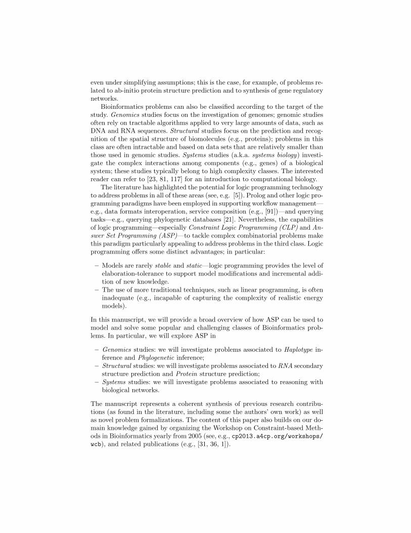
Fig. 2. Example of RNA secondary structure.

The RNA string r folds in the space according to a series of favorable matchesbetween pairs of nucleotides (base pairing). In this case, the presence of a singlestrand allows richer shapes w.r.t. the DNA helix. The so-called RNA secondarystructure is the set of its base pairings (see, for example, Figure 2). In particular,A–U and C–G are the favored base pairings; these are also known as the Watson-Crick pairs. Note that it is also possible to find U–G pairs. The topology of thepairs influences and stabilizes the three dimensional functional shape of thestrand. Predicting such three dimensional shape is extremely important, and

1 http://web.ornl.gov/sci/techresources/Human_Genome/

this is the topic of Section 5. It is interesting to note that, unlike the proteincase, an accurate secondary structure prediction for RNA is sufficient to inferthe overall three dimensional shape of the strand.

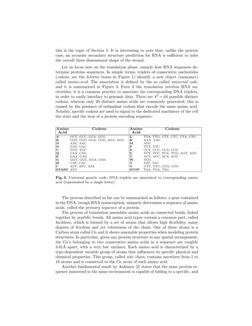
Let us focus now on the translation phase, namely how RNA sequences de-termine proteins sequences. In simple terms, triplets of consecutive nucleotides(codons, see the 3-letter boxes in Figure 1) identify a new object (monomer)called amino-acid. The association is defined by the so called universal code,and it is summarized in Figure 3. Even if the translation involves RNA nu-cleotides, it is a common practice to associate the corresponding DNA triplets,in order to easily interface to genomic data. There are 43 = 64 possible distinctcodons, whereas only 20 distinct amino acids are commonly generated; this iscaused by the presence of redundant codons that encode the same amino acid.Notably, specific codons are used to signal to the dedicated machinery of the cellthe start and the stop of a protein encoding sequence.

Amino Codons Amino CodonsAcid Acid

A GCT, GCC, GCA, GCG L TTA, TTG, CTT, CTC, CTA, CTGR CGT, CGC, CGA, CGG, AGA, AGG K AAA, AAGN AAT, AAC M ATGD GAT, GAC F TTT, TTCC TGT, TGC P CCT, CCC, CCA, CCGQ CAA, CAG S TCT, TCC, TCA, TCG, AGT, AGCE GAA, GAG T ACT, ACC, ACA, ACGG GGT, GGC, GGA, GGG W TGGH CAT, CAC Y TAT, TACI ATT, ATC, ATA V GTT, GTC, GTA, GTGSTART ATG STOP TAA, TGA, TAG

Fig. 3. Universal genetic code: DNA triplets are associated to corresponding aminoacid (represented by a single letter)

The process described so far can be summarized as follows: a gene containedin the DNA, trough RNA transcription, uniquely determines a sequence of aminoacids, called the primary sequence of a protein.

The process of translation assembles amino acids as connected beads, linkedtogether by peptidic bonds. All amino acid types contain a common part, calledbackbone, which is formed by a set of atoms that allows high flexibility, manydegrees of freedom and yet robustness of the chain. One of these atoms is aCarbon atom called Cα and it shows amenable properties when modeling proteinstructures. In particular, given any protein structure in any spatial arrangement,the Cα’s belonging to two consecutive amino acids in a sequence are roughly3.81A apart, with a very low variance. Each amino acid is characterized by atype-dependent variable group of atoms that influences its specific physical andchemical properties. This group, called side chain, contains anywhere from 1 to18 atoms and is connected to the Cα atom of each amino acid.

Another fundamental result by Anfinsen [2] states that the same protein se-quence immersed in the same environment is capable of folding to a specific, and

often stable, three dimensional shape, called the native state or native confor-mation. The process is spontaneous and arranges the molecule according to itsminimal free energy. The spatial arrangement of the protein, thanks to the chem-ical properties of amino acids on the surface, determines the function and howthe protein interacts and binds to other molecules (ligands). Thus, the combi-nation of the previously discussed central dogma and the properties of proteinsprovides the fundamental explanation of how a gene expressed by DNA canencode a protein that is capable of performing specific functions.

Proteins can contain from as few as 10 amino acids all the way to 1, 000 aminoacids. An average globular protein is about 300 amino acids long. Each aminoacid contains 7–24 atoms; therefore, the number possible arrangements of atomsin the three dimensional space is well beyond any computational power. Giventhe atomic size of proteins and the difficulties to experimentally determine theirnative state, the prediction of their structure plays a crucial role. This problemis discussed in Section 6.

When studying a living cell and/or organism, we need to contend with theexistence of a complex network of (partially known) interactions among the vari-ous active components. It is often the case that these interactions are not studiedat the lowest level of atomic-level processes, but the are instead abstracted usinghigher level perspectives. This is often necessary to address the high computa-tional complexity underlying these systems and the relatively limited knowledgeabout the interaction models. Depending of the level of simplification adopted,it is possible to investigate different properties of a system of cells and/or organ-isms. For example, metabolism, some signaling pathways of hormones and cellcycles can be modeled by fusing experimental data and stochastic analyses.

Systems biology describes the relationships among components through graphsand provides some computational models that can be used to reproduce particu-lar behaviors. The typical objects modeled are genes and DNA/RNA fragments,proteins and enzymes, metabolites and external stimuli. The goals of systemsbiology are to (a) analyze the network of interactions, (b) predict the behaviorof the system under specific conditions, and (c) integrate knowledge by mergingdiverse experimental data. The representation in use can vary, depending onthe scope and granularity of the modeled system: a specific reaction chain mayinvolve a few molecule types, a larger scale system may describe a cell behaviorthat involves genes expressions (e.g., quantity of RNA transcribed from a spe-cific gene in a time unit), while a very large system may describe a completeorganism with a more coarse description of single cell activities. Some techniquesdeveloped within the logic programming community to deal with problems fromsystems biology are presented in Section 7.

3 Phylogenetics

Phylogenies are artifacts used to describe the relationships among entities (e.g.,biological entities like proteins or genomes) derived from a process of evolution.

We often refer to the entities studies in a phylogeny as taxonomic units (TUs)or, simply, as Taxas.

The field of Phylogenetics developed from the domain of biology, as a powerfulinstrument to investigate similarities and differences among entities as a resultof an evolutionary process. Evolutionary theory provides a powerful frameworkfor comparative biology, by converting similarities and differences into eventsreflecting causal processes. As such, evolutionary-based methods provide morereliable answers than the traditional similarity-based methods, as they employa theory (of evolution) to describe changers instead of relying on simple patternmatching. Indeed, evolutionary analyses have become the norm in a variety ofareas of biological analysis. Evolutionary methods have proved successful, notmerely in addressing issues of interest to evolutionary biologists, but in regardto practical problems of structural and functional inference [107]. Evolutionaryinference of pairing interactions determining ribosomal RNA structure [116] is aclear case in which progress was made by the preferential use of an evolutionaryinference method, even when direct (but expensive and imprecise) experimentalalternatives were available. Eisen and others [101, 82] have shown how an explic-itly evolutionary approach to protein “function” assignment eliminates certaincategories of error that arise from gene duplication and loss, unequal rates ofevolution, and inadequate sampling. Other inference problems that have been ad-dressed through evolutionary methods include studies of implications of SNPs inthe human population [101], identification of specificity-determining sites [66],inference of interactions between sites in proteins [109], interactions betweenproteins [108], and inferences of categories of sets of genes that have undergoneadaptive evolution in recent history [83].

Phylogenetic analysis has also found applications in domains that are outsideof the realm of biology; for example, a rich literature has explored the evolutionof languages (e.g., [62, 94, 102, 42]).

3.1 Modeling

A phylogenetic tree (or simply a phylogeny) is typically a labeled binary tree(V,E, L, T ,L) where:

• The leaves L represent the taxonomic units being compared;

• The internal nodes V \L represent the (hypothetical) ancestral units; in rarecases, the internal nodes correspond to concrete entities (e.g., fossils);

• The edges E of the tree describe evolutionary relationships; the structure ofthe edges describe the processes that hypothetically led to the evolution ofthe TUs, e.g., biological processes of speciation, gene duplication, and geneloss;

• Commonly, each TU is described by a collection of finite domain proper-ties, referred to as characters. In the formalization, T = (C,D, f) is thedescription of such properties, where

− C = {c1, . . . , ck} is a finite set of characters;

− D = (Dc1 , . . . , Dck) associates a finite domain to each character;2

− f : L × C →⋃

c∈C Dc is a function that provides the value of eachcharacter for each TU being studied.

• We are often interested in the length of the branches of a phylogeny and/orthe assignment of dates to the internal nodes of the phylogeny; if this featureis present, then we will describe it as a function L : E → R+.

Whenever we do not have information about length of branches, we omit thecomponent L from the description of the phylogeny.

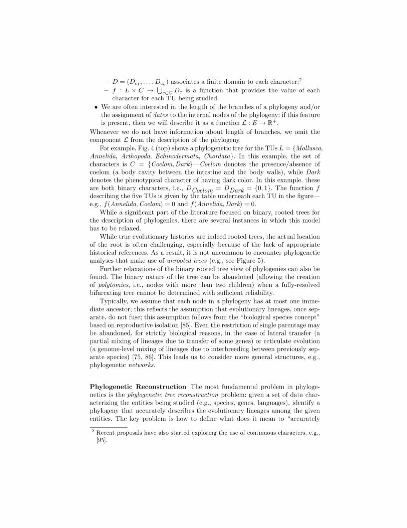
For example, Fig. 4 (top) shows a phylogenetic tree for the TUs L = {Mollusca,Annelida, Arthopoda, Echinodermata, Chordata}. In this example, the set ofcharacters is C = {Coelom,Dark}—Coelom denotes the presence/absence ofcoelom (a body cavity between the intestine and the body walls), while Darkdenotes the phenotypical character of having dark color. In this example, theseare both binary characters, i.e., DCoelom = DDark = {0, 1}. The function fdescribing the five TUs is given by the table underneath each TU in the figure—e.g., f(Annelida,Coelom) = 0 and f(Annelida,Dark) = 0.

While a significant part of the literature focused on binary, rooted trees forthe description of phylogenies, there are several instances in which this modelhas to be relaxed.

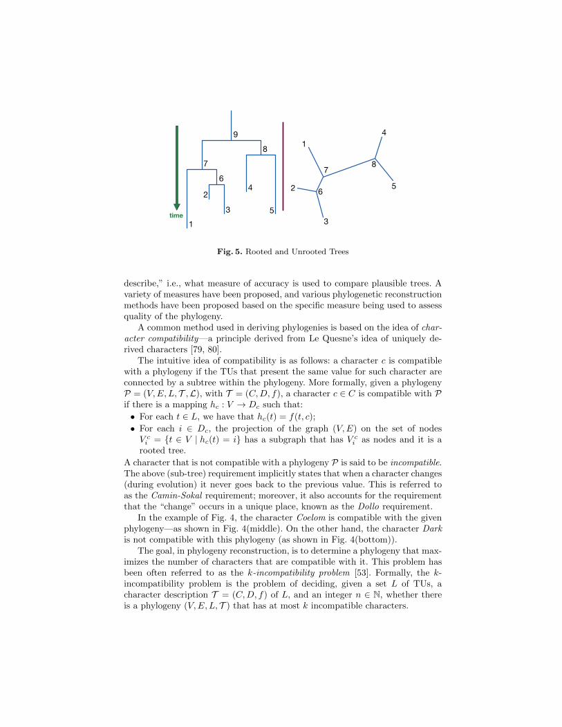
While true evolutionary histories are indeed rooted trees, the actual locationof the root is often challenging, especially because of the lack of appropriatehistorical references. As a result, it is not uncommon to encounter phylogeneticanalyses that make use of unrooted trees (e.g., see Figure 5).

Further relaxations of the binary rooted tree view of phylogenies can also befound. The binary nature of the tree can be abandoned (allowing the creationof polytomies, i.e., nodes with more than two children) when a fully-resolvedbifurcating tree cannot be determined with sufficient reliability.

Typically, we assume that each node in a phylogeny has at most one imme-diate ancestor; this reflects the assumption that evolutionary lineages, once sep-arate, do not fuse; this assumption follows from the “biological species concept”based on reproductive isolation [85]. Even the restriction of single parentage maybe abandoned, for strictly biological reasons, in the case of lateral transfer (apartial mixing of lineages due to transfer of some genes) or reticulate evolution(a genome-level mixing of lineages due to interbreeding between previously sep-arate species) [75, 86]. This leads us to consider more general structures, e.g.,phylogenetic networks.

Phylogenetic Reconstruction The most fundamental problem in phyloge-netics is the phylogenetic tree reconstruction problem: given a set of data char-acterizing the entities being studied (e.g., species, genes, languages), identify aphylogeny that accurately describes the evolutionary lineages among the givenentities. The key problem is how to define what does it mean to “accurately

2 Recent proposals have also started exploring the use of continuous characters, e.g.,[95].

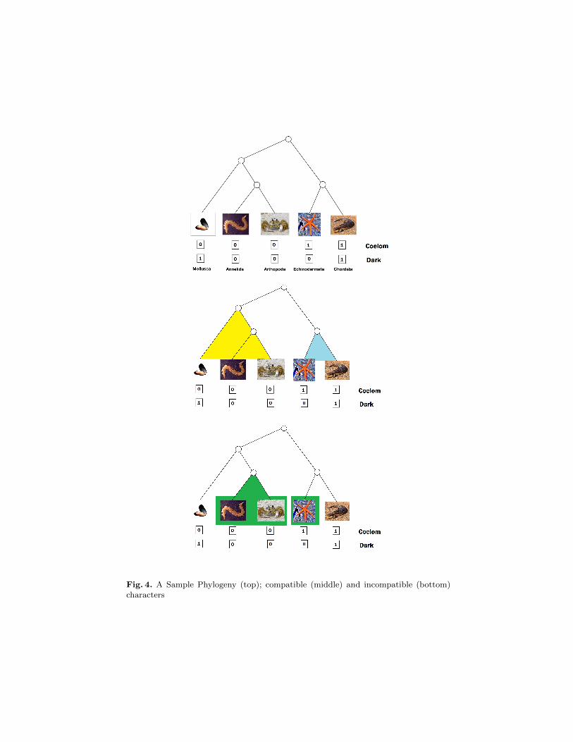
Fig. 4. A Sample Phylogeny (top); compatible (middle) and incompatible (bottom)characters

1

23

4

5

67

89

time

1

2

3

6

7 8

5

4

Fig. 5. Rooted and Unrooted Trees

describe,” i.e., what measure of accuracy is used to compare plausible trees. Avariety of measures have been proposed, and various phylogenetic reconstructionmethods have been proposed based on the specific measure being used to assessquality of the phylogeny.

A common method used in deriving phylogenies is based on the idea of char-acter compatibility—a principle derived from Le Quesne’s idea of uniquely de-rived characters [79, 80].

The intuitive idea of compatibility is as follows: a character c is compatiblewith a phylogeny if the TUs that present the same value for such character areconnected by a subtree within the phylogeny. More formally, given a phylogenyP = (V,E, L, T ,L), with T = (C,D, f), a character c ∈ C is compatible with Pif there is a mapping hc : V → Dc such that:

• For each t ∈ L, we have that hc(t) = f(t, c);

• For each i ∈ Dc, the projection of the graph (V,E) on the set of nodesV ci = {t ∈ V | hc(t) = i} has a subgraph that has V c

i as nodes and it is arooted tree.

A character that is not compatible with a phylogeny P is said to be incompatible.The above (sub-tree) requirement implicitly states that when a character changes(during evolution) it never goes back to the previous value. This is referred toas the Camin-Sokal requirement; moreover, it also accounts for the requirementthat the “change” occurs in a unique place, known as the Dollo requirement.

In the example of Fig. 4, the character Coelom is compatible with the givenphylogeny—as shown in Fig. 4(middle). On the other hand, the character Darkis not compatible with this phylogeny (as shown in Fig. 4(bottom)).

The goal, in phylogeny reconstruction, is to determine a phylogeny that max-imizes the number of characters that are compatible with it. This problem hasbeen often referred to as the k-incompatibility problem [53]. Formally, the k-incompatibility problem is the problem of deciding, given a set L of TUs, acharacter description T = (C,D, f) of L, and an integer n ∈ N, whether thereis a phylogeny (V,E, L, T ) that has at most k incompatible characters.

Remark 1. We report on some combinatorial considerations. Given a set of nTUs, the number of unrooted trees can be computed by the formula (using theso-called double-factorial) (2n−5)!! = 1 ·3 ·5 · · · · ·2n−5, while while the numberof rooted trees is (2n−3)!! = 1 ·3 ·5 · · · · ·2n−3. As such, the number of possiblephylogenies is exponential in the number of TUs given.

The problem considered above, based on k-incompatibility, has been studiedin the literature and determined to be NP-complete [39]. The proof relies on areduction of the k-clique problem to the k-incompatibility problem. This resultis not surprising, and similar complexity results can be found for other measuresof phylogeny accuracy—e.g., the popular maximum parsimony method for theconstruction of phylogenies is shown to be NP-hard in [38].

3.2 ASP Encoding

The k-incompatibility problem admits an elegant encoding in ASP, thanks to itsnatural formulation as a generate-and-test problem.

Let us assume that the TUs for the problem at hand are represented in ASPas a collection of facts of the form taxa(i) where i is the name of a TU. Forthe sake of simplicity, let us assume that the TUs have been numbered andwe use the index of a TU as its name—thus, we will use the ASP declaration

taxa(1..N).

where N is the number of TUs. The character description T will be providedextensionally using facts of the form:

character(c). %% For each c ∈ Cdomain(c, s). %% For each s ∈ Dc

f(i, c, v). %% For each i ∈ L, c ∈ C such that f(i, c) = v

The code is divided in two parts: the tree construction and the computationof hc. Let us focus on the tree construction first:

(1) num_of_taxas(N) :- N = #count{taxa(L)}.

(2) node(1..2*N-1) :- num_of_taxas(N).

% Each internal node has exactly two children

(3) 2 { edge(I,J): node(J)} 2 :- node(I), not taxa(I).

% Children are of smaller index

(4) :- node(I;J), edge(I,J), I < J.

% Each node but the root has 1 fathers

(5) 1 { edge(I,J): node(I) } 1 :- node(J), num_of_taxas(N), J < 2*N-1.

Nodes 1 to N are used for the TUs and they represent leaves of the tree beingconstructed. The tree has 2N − 1 nodes and node 2N − 1 is the root. Lines (1)and (2) compute the number of TUs and define the nodes of the trees. Line (3)is used to enforce the binary structure of the tree (each internal node has exactlytwo children) and to ensure that the TUs are appearing as leaves of the tree.Line (4) is used to ensure that edges point from bigger to smaller nodes, allowing

us to remove symmetries. Finally, line (5) allows us to ensure the creation of atree, by verifying that each node, except for the root, has exactly one parent.

The second part of the code is used to assess the compatibility of the phy-logeny with respect to the characters.

% h_c (i.e., h(_,C,_)) is a total function

(6) 1 { h(I,C,V): domain(C,V) } 1 :- node(I), character(C).

% h_c is an extension of f

(7) h(I,C,V) :- taxa(I), f(I,C,V).

% Project the tree on each character

(8) char_edge(C,V,A,B) :- node(A;B), domain(C,V),

edge(A,B), h(A,C,V), h(B,C,V).

% A node can be either a root or not after the projection

(9) no_root(C,V,A) :- node(A;B), domain}(C,V), h(A,C,V),

char_edge(C,V,B,A).

(10) root(C,V,A) :- node(A), domain(C,V), h(A,C,V), not no_root(C,V,A).

% If there are two roots, it is not partially compatible

(11) two_roots(C,V) :- node(A;B), A < B, domain(C,V),

root(C,V,A), root(C,V,B).

(12) partially_compatible(C,V) :- domain(C,V), not two_roots(C,V).

% If for all symbols is partially_compatible, it is compatible

(13) compatible(C) :- character(C).

(14) :- character(C), compatible(C), domain(C,V),

not partially_compatible(C,V).

% Maximize the compatible characters

(15) compats(N) :- N = #count{ compatible(C) }.

(16) #maximize [ compats(N)=N ].

Lines (6) and (7) provide the definition of the function hc, ensuring thatit represents an extension of f . The code in line (8) extracts the edges of thephylogeny that link nodes with the same value for a given character. This cre-ates a new tree, composed of edges labeled by the pair (c, v) of character andcorresponding value. The projected trees are analyzed to determine whetherthey represent individual trees or forests (lines (11)-(13)). If there are multipletrees for the same (c, v), then the phylogeny is incompatible for such charactervalue. Lines (15) and (16) allow us to classify the phylogeny with respect to eachcharacter—as being compatible or not. Finally, Line (18) forces the search forphylogenies that maximize the number of compatible characters.

Remark 2. In the encoding above and in all encodings in the paper we modeledthe optimization version of the problem. In general, for encoding a decisionversion, i.e. is there a solution of size at least (at most) k one have to replacethe last two lines of the encodings with a line of the kind:

k { compatible(C) : character(C) }.

where k can be given as input (e.g., -c k=2)—k should be on the right forrequiring at most.

3.3 Related work

The use of logic programming in the context of phylogenetic inference is a rela-tively new domain.

Erdem an her collaborators have extensively studied several variants of thephylogeny reconstruction problem, both using traditional Answer Set Program-ming, as well as more ad-hoc logic programming systems. A nice survey of theircontributions can be found in [48]. The ASP modeling of phylogenetic reconstruc-tion using the k-incompatibility problem was originally proposed in [11, 10], laterexpanded to address issues of polymorphic characters. This line of work was laterextended to address the problem of formulating criteria of diversity or similarityin the generation of phylogenies, enabling the creation of pools of phylogeniesthat are sufficiently similar/dissimilar [14]; similarly, the problem of dealing withlarge numbers of plausible solutions has been addressed in [15] using mechanismsto weight each phylogeny.

The proposed solution described in the previous section is not suitable todeal with very large data sets; techniques based on divide-and-conquer have beensuccessfully adopted to the problem of phylogeny reconstruction [10, 13]; similarideas have been used in other areas associated to manipulation of phylogeneticknowledge (e.g., for supertree construction [100]).

The study of phylogenies that include time calibrations has been first con-sidered in [50, 51], with special considerations for how to deal with real-valuedtime stamps and even larger data sets.

Another line of research focused on the application of logic programmingtechnology to phylogenetic analysis and, more in general, to phyloinformatics,can be found in the context of the CDAOStore project [78, 21]. The CDAOS-tore relies on a triple-based encoding of phylogenetic artifacts (predominantlyphylogenies and associated character data matrices), encoded using the Com-parative Data Analysis Ontology (CDAO) [92]. Logic programming is employed,in CDAOStore, to implement a variety of queries to a phylogenetic repository,including structural queries (to retrieve phylogenies that meet certain structuralconstraints) and synthesis queries (e.g., to develop supertrees of sets of collectedphylogenies).

4 Haplotype Inference

The DNA of diploid organisms, such as humans, is organized in pairs of notcompletely identical copies of chromosomes. The sequence of nucleotides from asingle copy is called haplotype, while the conflation of the two copies constitutesa genotype. Each person inherits one of the two haplotypes from each parent.The most common variation between two haplotypes is a difference in a singlenucleotide. Using statistical analysis within a population, it is possible to de-scribe and analyze the typical points where these mutations occur. Each of suchdifferences is called a Single Nucleotide Polymorphism (SNP). In other words, aSNP is a single nucleotide site, in the DNA sequence, where more than one type

of nucleotide (usually two) occur with a non-negligible population frequency. Werefer to such sites as alleles.

Considering a specific genotype, a SNP site where the two haplotypes havethe same nucleotide is called an homozygous site, while it is heterozygous other-wise. Research has confirmed that SNPs are the most common and predominantform of genetic variation in DNA. Moreover, SNPs can be linked to specific traitsof individuals and with their phenotypic variations within their population. Con-sequently, haplotype information in general, and SNPs in particular, are relevantin several contexts, such as, for instance, in the study and diagnosis of geneticdiseases, in forensic applications, etc. This makes the identification of the hap-lotype structure of individuals, as well as the common part within a population,of crucial importance. However, in practice, biological experiments are used tocollect directly genotype data instead of haplotype data, mainly due to cost ortechnological limitations. To overcome such limitations, efficient and accuratecomputational methods for inferring haplotype information from genotype datahave been developed during the last decades (for a review, the reader is referredto [72, 69, 70]).

4.1 Modeling

The haplotype inference problem can be formulated as follows. First, we apply anabstraction and represent genotypes and haplotypes by focusing on the collectionof ambiguous SNPs sites in a population. Moreover, let us denote, for each site,the two possible alleles using 0 and 1, respectively. Hence, an haplotype will berepresented by a sequence of n components taken from {0, 1}. Each genotypeg, being a conflation of two (partially) different haplotypes h1 and h2, will berepresented as a sequence of n elements taken from {0, 1, 2}, such that 0 and 1are used for its homozygous sites, while 2 is used for the heterozygous sites.

More specifically, following [77], let us define the conflation operation g =h1 ⊕ h2 as follows:

g[i] =

{h1[i] if h1[i] = h2[i]2 otherwise

where g[i] denotes the ith element of the sequence g, for i = 1, . . . , n.We say that a genotype g is resolved by a pair of haplotypes h1 and h2 if

g = h1 ⊕ h2. A set H of haplotypes explains a given set G of genotypes, if foreach g ∈ G there exists a pair of haplotypes h1, h2 ∈ H such that g = h1 ⊕ h2.

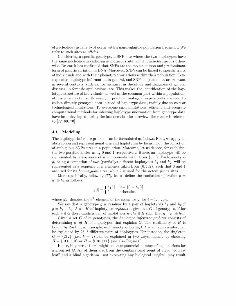
Given a set G of m genotypes, the haplotype inference problem consists ofdetermining a set H of haplotypes that explains G. The cardinality of H isbound by 2m but, in principle, each genotype having k ≤ n ambiguous sites, canbe explained by 2k−1 different pairs of haplotypes. For instance, the singletonG = {212} (i.e., k = 2) can be explained in two ways, namely by choosingH = {011, 110} or H = {010, 111} (see also Figure 6).

Hence, in general, there might be an exponential number of explanations fora given set G. All of them are, from the combinatorial point of view, “equiva-lent” and a blind algorithm—not exploiting any biological insight—may result

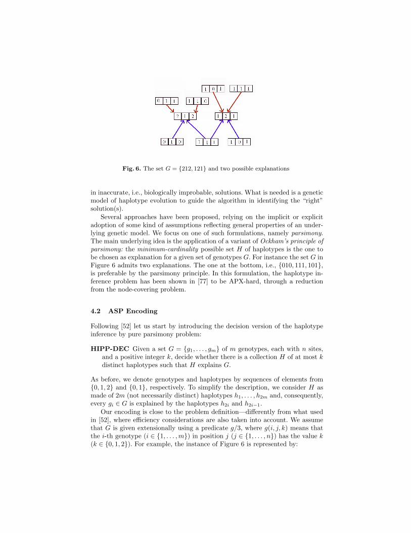
Fig. 6. The set G = {212, 121} and two possible explanations

in inaccurate, i.e., biologically improbable, solutions. What is needed is a geneticmodel of haplotype evolution to guide the algorithm in identifying the “right”solution(s).

Several approaches have been proposed, relying on the implicit or explicitadoption of some kind of assumptions reflecting general properties of an under-lying genetic model. We focus on one of such formulations, namely parsimony.The main underlying idea is the application of a variant of Ockham’s principle ofparsimony: the minimum-cardinality possible set H of haplotypes is the one tobe chosen as explanation for a given set of genotypes G. For instance the set G inFigure 6 admits two explanations. The one at the bottom, i.e., {010, 111, 101},is preferable by the parsimony principle. In this formulation, the haplotype in-ference problem has been shown in [77] to be APX-hard, through a reductionfrom the node-covering problem.

4.2 ASP Encoding

Following [52] let us start by introducing the decision version of the haplotypeinference by pure parsimony problem:

HIPP-DEC Given a set G = {g1, . . . , gm} of m genotypes, each with n sites,and a positive integer k, decide whether there is a collection H of at most kdistinct haplotypes such that H explains G.

As before, we denote genotypes and haplotypes by sequences of elements from{0, 1, 2} and {0, 1}, respectively. To simplify the description, we consider H asmade of 2m (not necessarily distinct) haplotypes h1, . . . , h2m and, consequently,every gi ∈ G is explained by the haplotypes h2i and h2i−1.

Our encoding is close to the problem definition—differently from what usedin [52], where efficiency considerations are also taken into account. We assumethat G is given extensionally using a predicate g/3, where g(i, j, k) means thatthe i-th genotype (i ∈ {1, . . . ,m}) in position j (j ∈ {1, . . . , n}) has the value k(k ∈ {0, 1, 2}). For example, the instance of Figure 6 is represented by:

g(1,1,2). g(1,2,1). g(1,3,2).

g(2,1,1). g(2,2,2). g(2,3,1).

Moreover, the domain predicates geno(1..m), site(1..n), haplo(1..2m) are alsopart of the input. In the current example we have:

geno(1..2). site(1..3). haplo(1..4).

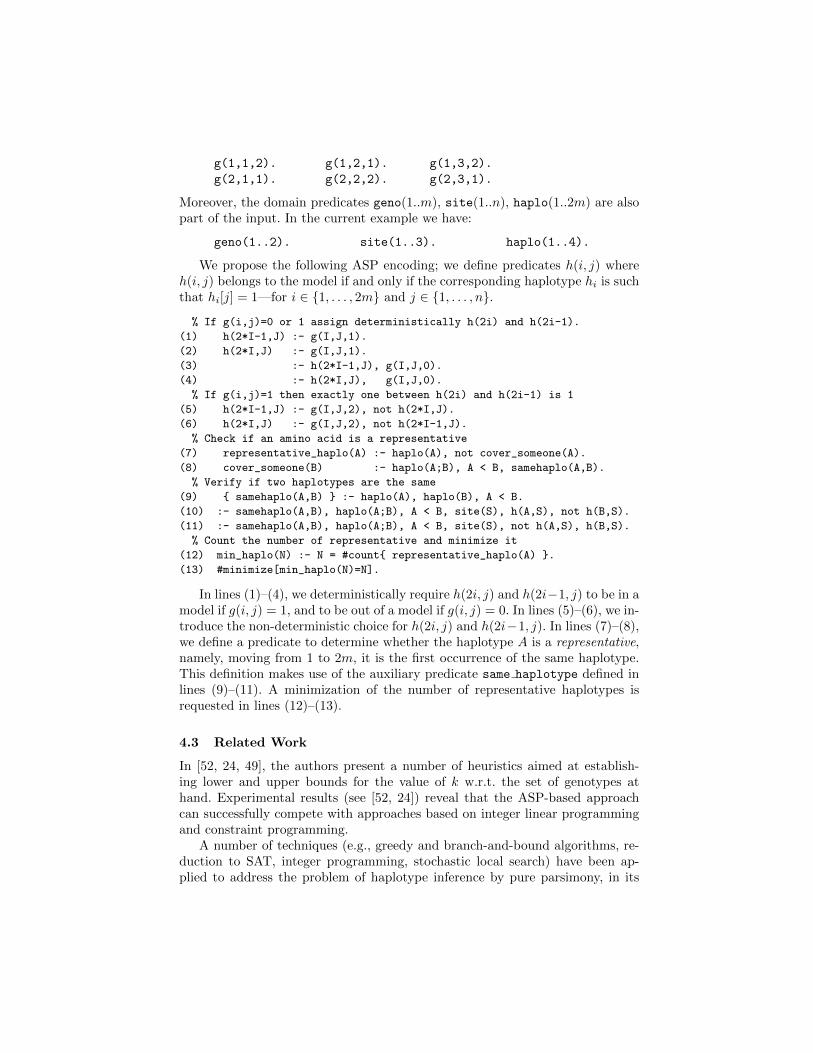
We propose the following ASP encoding; we define predicates h(i, j) whereh(i, j) belongs to the model if and only if the corresponding haplotype hi is suchthat hi[j] = 1—for i ∈ {1, . . . , 2m} and j ∈ {1, . . . , n}.

% If g(i,j)=0 or 1 assign deterministically h(2i) and h(2i-1).

(1) h(2*I-1,J) :- g(I,J,1).

(2) h(2*I,J) :- g(I,J,1).

(3) :- h(2*I-1,J), g(I,J,0).

(4) :- h(2*I,J), g(I,J,0).

% If g(i,j)=1 then exactly one between h(2i) and h(2i-1) is 1

(5) h(2*I-1,J) :- g(I,J,2), not h(2*I,J).

(6) h(2*I,J) :- g(I,J,2), not h(2*I-1,J).

% Check if an amino acid is a representative

(7) representative_haplo(A) :- haplo(A), not cover_someone(A).

(8) cover_someone(B) :- haplo(A;B), A < B, samehaplo(A,B).

% Verify if two haplotypes are the same

(9) { samehaplo(A,B) } :- haplo(A), haplo(B), A < B.

(10) :- samehaplo(A,B), haplo(A;B), A < B, site(S), h(A,S), not h(B,S).

(11) :- samehaplo(A,B), haplo(A;B), A < B, site(S), not h(A,S), h(B,S).

% Count the number of representative and minimize it

(12) min_haplo(N) :- N = #count{ representative_haplo(A) }.

(13) #minimize[min_haplo(N)=N].

In lines (1)–(4), we deterministically require h(2i, j) and h(2i−1, j) to be in amodel if g(i, j) = 1, and to be out of a model if g(i, j) = 0. In lines (5)–(6), we in-troduce the non-deterministic choice for h(2i, j) and h(2i−1, j). In lines (7)–(8),we define a predicate to determine whether the haplotype A is a representative,namely, moving from 1 to 2m, it is the first occurrence of the same haplotype.This definition makes use of the auxiliary predicate same haplotype defined inlines (9)–(11). A minimization of the number of representative haplotypes isrequested in lines (12)–(13).

4.3 Related Work

In [52, 24, 49], the authors present a number of heuristics aimed at establish-ing lower and upper bounds for the value of k w.r.t. the set of genotypes athand. Experimental results (see [52, 24]) reveal that the ASP-based approachcan successfully compete with approaches based on integer linear programmingand constraint programming.

A number of techniques (e.g., greedy and branch-and-bound algorithms, re-duction to SAT, integer programming, stochastic local search) have been ap-plied to address the problem of haplotype inference by pure parsimony, in its

initial formulation as well as in a number of variants and refinements, such as[12, 18, 24, 40, 64, 65, 99, 115, 118]. Among the various proposals appearing inliterature, we mention the rule-based method proposed by Clark [22], which inits general form suffers from the NP-hardness of the problem.

Several alternative principles, different from parsimony, have also been ex-plored. One of them is called the infinite sites model. It postulates that, duringthe evolution of a population, a mutation that results in a SNP occurs onlyonce in the history; this reflects the Dollo and Camin-Sokal principles discussedin the previous section. Hence, all individuals sharing a specific allele must bedescendants of a single ancestor.

Methods relying on maximum likelihood criteria assume that the probabilityof observing a genotype is strictly related to the probability of observing itsconstituent haplotypes. Hence, these methods estimate the probability of (eachspecific set H of) haplotypes from observed genotypes frequencies in the realpopulation. These methods seek the most probable solution.

Other methods make hypotheses on the historical evolution of the charac-ters in a population. The notion of perfect phylogeny is introduced to representsuch evolution as a rooted tree (coalescent model, see [68]). The tree-structurenot only imposes constraints on the candidate solutions, but also reduces thecomputational complexity of the problem.

For a much detailed treatment of these and other methods, we refer theinterested reader to [72, 70] and to the references therein.

5 RNA secondary structure prediction

In this chapter, we focus on the prediction of the secondary structure arrange-ment for RNA strands. We provide a model for a simplified version of the problemand we show an elegant ASP encoding.

As anticipated in Section 2, an RNA sequence S = s1 · · · sn is a string ofsymbols from {A,C,G,U}. The sequence can fold in the space, so that pairsof bases can physically interact. The secondary structure can be described by aset of pairs of interacting bases. In Figure 7, we show an example of an RNAsequence and a set of pairs of bases (denoted by solid lines). In general, theenergetic evaluation of these interactions can be computed in a precise way, re-gardless of the overall three dimensional arrangement of the sequence. Therefore,it is possible to compute the best secondary structure while ignoring the actualfolding in space. This gives rise to specific prediction algorithms that are muchmore reliable when compared to the prediction tools for amino acid sequences(see also Section 6).

In order to identify the most probable secondary structure, various energeticmodels have been studied and efficient methods for its estimation have been pro-posed. In the following, we present two simple approximations of energy func-tions. The first one is based of the simplest approximation and maximizes thenumber of favorable pairings (i.e., A–U , C–G, and U–G). A more refined energyfunction scores the frequency of the pairs.

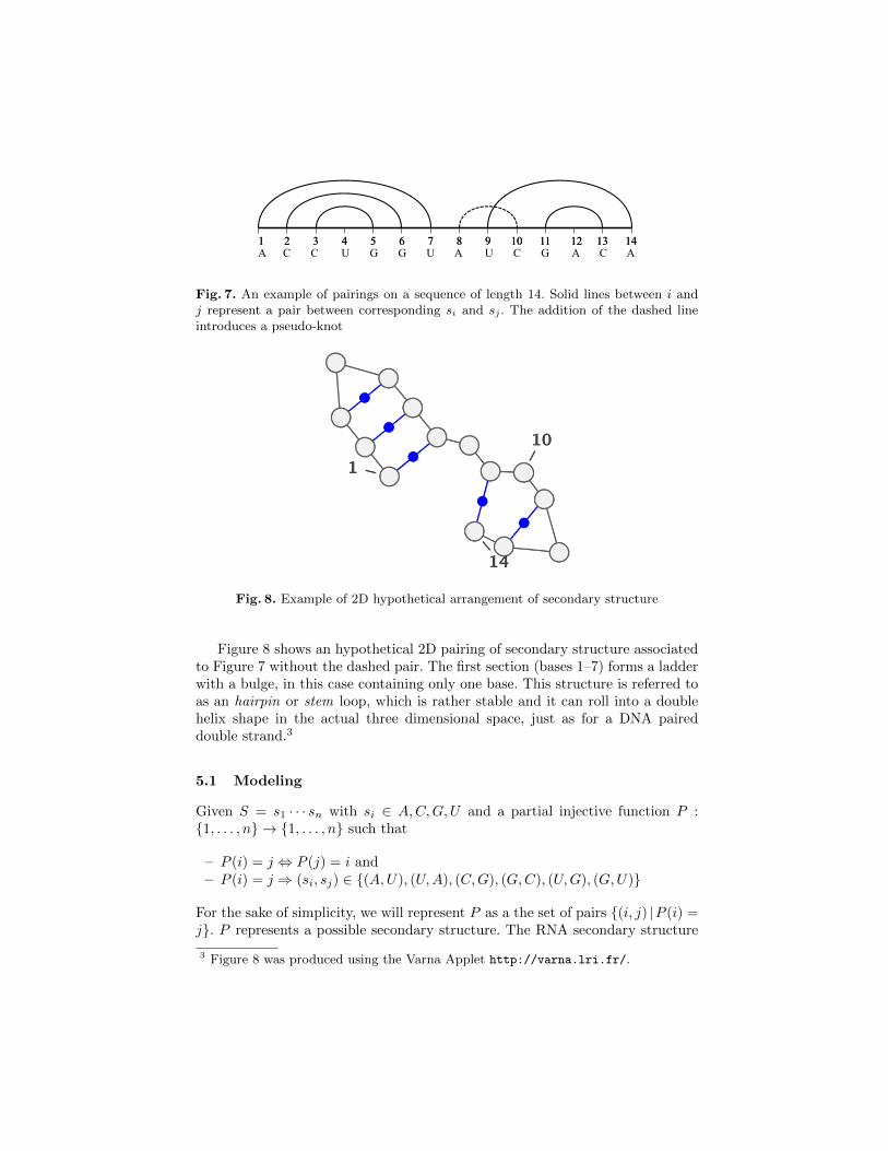
1 2 3 4 5 6 7 8 9 10 11 12 13 141 2 3 4 5 6 7 8 9 10 11 12 13 14A C C U G G U A U C G A C A

Fig. 7. An example of pairings on a sequence of length 14. Solid lines between i andj represent a pair between corresponding si and sj . The addition of the dashed lineintroduces a pseudo-knot

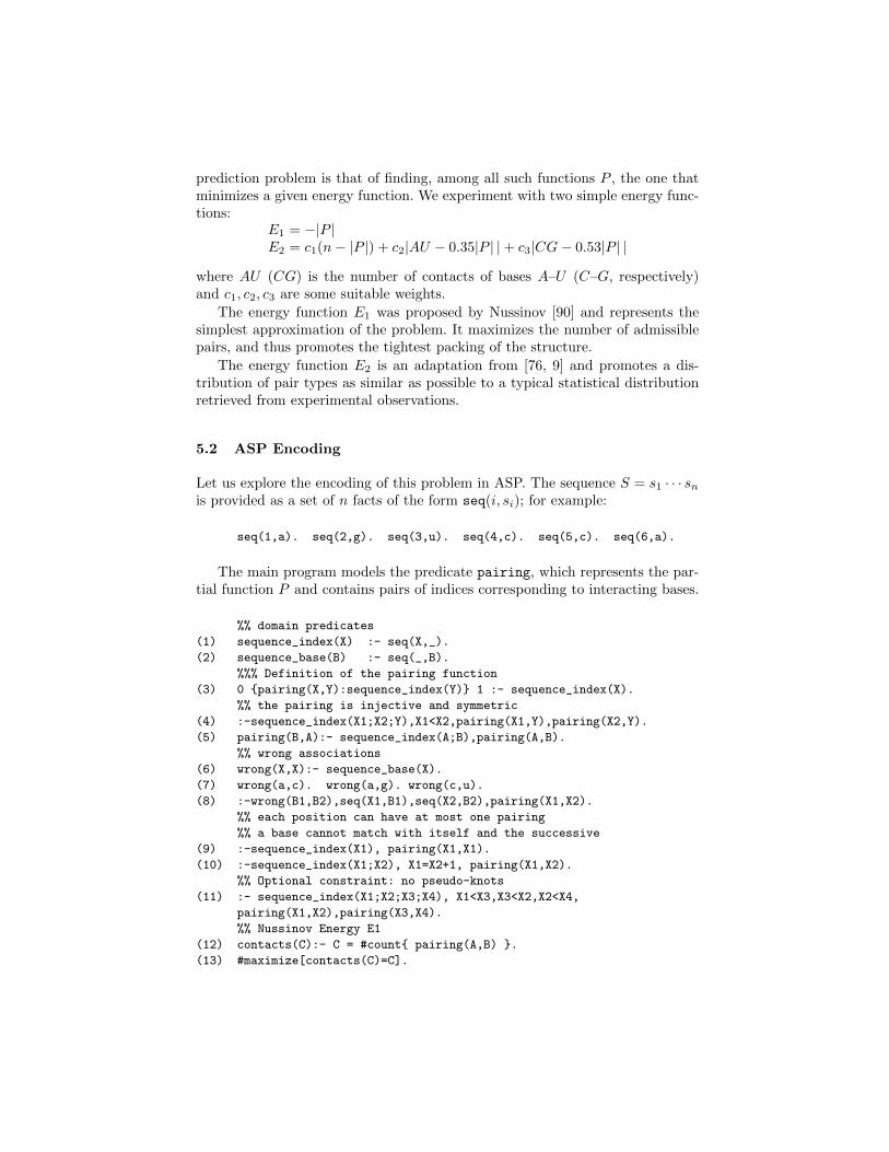
Fig. 8. Example of 2D hypothetical arrangement of secondary structure

Figure 8 shows an hypothetical 2D pairing of secondary structure associatedto Figure 7 without the dashed pair. The first section (bases 1–7) forms a ladderwith a bulge, in this case containing only one base. This structure is referred toas an hairpin or stem loop, which is rather stable and it can roll into a doublehelix shape in the actual three dimensional space, just as for a DNA paireddouble strand.3

5.1 Modeling

Given S = s1 · · · sn with si ∈ A,C,G,U and a partial injective function P :{1, . . . , n} → {1, . . . , n} such that

– P (i) = j ⇔ P (j) = i and– P (i) = j ⇒ (si, sj) ∈ {(A,U), (U,A), (C,G), (G,C), (U,G), (G,U)}

For the sake of simplicity, we will represent P as a the set of pairs {(i, j) |P (i) =j}. P represents a possible secondary structure. The RNA secondary structure

3 Figure 8 was produced using the Varna Applet http://varna.lri.fr/.

prediction problem is that of finding, among all such functions P , the one thatminimizes a given energy function. We experiment with two simple energy func-tions:

E1 = −|P |E2 = c1(n− |P |) + c2|AU − 0.35|P | |+ c3|CG− 0.53|P | |

where AU (CG) is the number of contacts of bases A–U (C–G, respectively)and c1, c2, c3 are some suitable weights.

The energy function E1 was proposed by Nussinov [90] and represents thesimplest approximation of the problem. It maximizes the number of admissiblepairs, and thus promotes the tightest packing of the structure.

The energy function E2 is an adaptation from [76, 9] and promotes a dis-tribution of pair types as similar as possible to a typical statistical distributionretrieved from experimental observations.

5.2 ASP Encoding

Let us explore the encoding of this problem in ASP. The sequence S = s1 · · · snis provided as a set of n facts of the form seq(i, si); for example:

seq(1,a). seq(2,g). seq(3,u). seq(4,c). seq(5,c). seq(6,a).

The main program models the predicate pairing, which represents the par-tial function P and contains pairs of indices corresponding to interacting bases.

%% domain predicates

(1) sequence_index(X) :- seq(X,_).

(2) sequence_base(B) :- seq(_,B).

%%% Definition of the pairing function

(3) 0 {pairing(X,Y):sequence_index(Y)} 1 :- sequence_index(X).

%% the pairing is injective and symmetric

(4) :-sequence_index(X1;X2;Y),X1<X2,pairing(X1,Y),pairing(X2,Y).

(5) pairing(B,A):- sequence_index(A;B),pairing(A,B).

%% wrong associations

(6) wrong(X,X):- sequence_base(X).

(7) wrong(a,c). wrong(a,g). wrong(c,u).

(8) :-wrong(B1,B2),seq(X1,B1),seq(X2,B2),pairing(X1,X2).

%% each position can have at most one pairing

%% a base cannot match with itself and the successive

(9) :-sequence_index(X1), pairing(X1,X1).

(10) :-sequence_index(X1;X2), X1=X2+1, pairing(X1,X2).

%% Optional constraint: no pseudo-knots

(11) :- sequence_index(X1;X2;X3;X4), X1<X3,X3<X2,X2<X4,

pairing(X1,X2),pairing(X3,X4).

%% Nussinov Energy E1

(12) contacts(C):- C = #count{ pairing(A,B) }.

(13) #maximize[contacts(C)=C].

The clauses in lines (1)–(2) extract domain knowledge from the input. Line(3) defines the partial function pairing, which is forced to be injective, bythe constraint in line (4), and symmetric, by the clause in line (5). Lines (6)–(8)discard non-admissible pairs, according to the definitions in the modeling section.The constraints in line (9) and (10) forbid the pairing of a base with itself andits neighbors. The constraint in line (11) enforces the absence of pseudo-knots(see Sect. 5.3). If this constraint is removed, then the program will model theNP-complete version of the problem. The clauses in lines (12) and (13) collectand minimize the number of contacts, respectively.

Let us briefly show how to encode the energy model E2. Line (13′) replacesthe optimization instruction (13) by asking for a minimal energy. The clausesin lines (14)–(16) define the count of the total number of AU and CG pairs inthe sequence, respectively. The energy predicate, in line (18), defines the energyfunction E2. We assign here c1 = c2 = c3 = 1. Note that the first coefficientand lines (22)–(23) are multiplied by 100 in order to scale from floating point tointeger numbers.

(13’) #maximize[energy(E)=E].

(14) total(N) :- N=#count{ seq(X,Y)}.

(15) au(N) :- N=#count{pairing(A,B):seq(A,a):seq(B,u)}.

(16) cg(N) :- N=#count{pairing(A,B):seq(A,c):seq(B,g)}.

(18) energy(E) :- C1=1, C2=1, C3=1,

total(N), contacts(C), au(AU), cg(CG),

E = C1 * (N-C/2) + C2 * #abs(100*AU - 35*C) +

C3 * #abs(100*CG - 53*C).

Let us observe that the latter version of the solution encounters significantgrounding problems, even for average size inputs.

5.3 Related work

In the literature, RNA secondary structure prediction has been addressed by alarge number of proposals, presenting different algorithms and various energyfunctions. Starting from the seminal work by Tinoco [110], where propensityof forming helices was addressed, other popular methods include the one byJacobson and Nussinov [90], introduced more than 30 years ago. It promotesthe maximal number of admissible pairs in the sequence. This approach can beaddressed by a polynomial dynamic programming approach for a restricted classof solutions (in absence of pseudo-knots, see the complexity notes below).

More refined energy functions have been proposed, with the specific goalto better estimate hairpin loops. The Zucker’s algorithm [119] proposes a moreprecise estimate of stacking pairs forming a hairpin loop, as well as contributionsfor opening and closing a loop. The computational complexity of the solution ispolynomial in absence of pseudo-knots, and non-logic programming techniques,i.e., dynamic programming, have been proposed. The original algorithm proposesan energy minimization approach.

Other energy functions have been proposed as the result of probabilisticanalyses. In particular, the mean distribution of base pairs found in actual RNAsecondary structures has been used as the target of the secondary structureprediction. The most favorable structure is the one that best approximates suchdistribution [76, 9].

In order to improve the structural results, Sankoff proposed a simultaneousalignment and folding approach, which goes beyond the scope of this section [96].

In the general case, the decisional version of the problem is NP-complete—see [84] for the original proof. The main idea is to reduce a 3-SAT formula intoa particular sequence such that there exists a specific number of contacts ifand only if the original formula is satisfiable. An interesting polynomial class ofproblems has been characterized by the absence of pseudo-knots (see dashed pairdrawn in Figure 7). A pseudo-knot is encountered when the following propertyholds: for two pairings (i, j) and (`, k) in P ,

i < ` < j ⇒ j < k ∨ k < i

The work in [8] provides examples of energy functions for general structures withpseudo-knots. Moreover, a constraint propagation approach for alignment andfolding in the presence of pseudo-knots has been presented in [37]. For pseudo-knot free structures, dynamic programming algorithms can be used with a timecomplexity ranging from O(n2) to O(n4), depending on the energy functionbeing considered, while space complexity ranges from O(n) to O(n2) .

6 Protein Structure Prediction

The problem we introduce here is a simplification of the protein structure pre-diction (PSP) problem. In particular, we consider two levels of simplification:

– Protein model: we consider only one atom per amino acid. Moreover, wepartition the 20 amino acids in two families: h (hydropic) and p (polar);

– Spatial model: we focus exclusively on a simple 2D discrete lattice represen-tation of the space.

We provide some more details on the full version of the problem and to (some)approaches for dealing with it in Subsection 6.3.

6.1 Modeling

We refer to such simplified version of the problem as the 2DHP-PSP. The prob-lem can be formulated in a simple way as follows. The input is a list of aminoacids S = s1 · · · sn, where si ∈ {h, p}. Imagine S as a pearl necklace, where thesis are the pearls, while the distance between si and si+1 is constant. This stringof pearls lays down on a large 2D matrix, where the size of the square is exactlythe distance among pearls—for the sake of simplicity, we will assume such dis-tance to be 1—with the further constraints that si must occupy the intersection

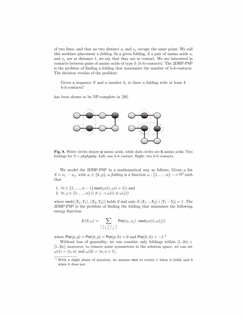
of two lines, and that no two distinct si and sj occupy the same point. We callthis necklace placement a folding. In a given folding, if a pair of amino acids siand sj are at distance 1, we say that they are in contact. We are interested incontacts between pairs of amino acids of type h (h-h-contacts). The 2DHP-PSPis the problem of finding a folding that maximizes the number of h-h-contacts.The decision version of the problem:

Given a sequence S and a number k, is there a folding with at least kh-h-contacts?

has been shown to be NP-complete in [29].

Fig. 9. White circles denote p amino acids, while dark circles are h amino acids. Twofoldings for S = phphpphp. Left: one h-h contact. Right: two h-h contacts.

We model the 2DHP-PSP in a mathematical way as follows. Given a listS = s1 · · · sn, with si ∈ {h, p}, a folding is a function ω : {1, . . . , n} −→ N2 suchthat

1. ∀i ∈ {1, . . . , n− 1} next(ω(i), ω(i+ 1)) and2. ∀i, j ∈ {1, . . . , n} (i 6= j → ω(i) 6= ω(j))

where next(〈X1, Y1〉, 〈X2, Y2〉) holds if and only if |X1−X2|+ |Y1−Y2| = 1. The2DHP-PSP is the problem of finding the folding that minimizes the followingenergy function:

E(S, ω) =∑

1 ≤ i ≤ n − 2i + 2 ≤ j ≤ n

Pot(si, sj) · next(ω(i), ω(j))

where Pot(p, p) = Pot(h, p) = Pot(p, h) = 0 and Pot(h, h) = −1.4

Without loss of generality, we can consider only foldings within [1..2n] ×[1..2n]; moreover, to remove some symmetries in the solution space, we can setω(1) = 〈n, n〉 and ω(2) = 〈n, n+ 1〉,

4 With a slight abuse of notation, we assume next to return 1 when it holds and 0when it does not.

Contiguous occurrences of h in the input sequence S (namely, when si =si+1 = h) contribute in the same way to the energy associated to each foldingand, thus, they are not considered in the objective function.

An easy observation (that unfortunately cannot be “lifted” to the generalPSP formulation) is that si and sj can be in contact only if j − i is odd.

6.2 ASP Encoding

The essential part of the ASP encoding of this problem is presented in [43].A specific instance S = s1, . . . , sn of the problem is represented by a set of nfacts of the kind prot(i, si). For instance, the protein phphpphp of Figure 9 isdescribed as:

prot(1,p). prot(2,h). prot(3,p). prot(4,h).

prot(5,p). prot(6,p). prot(7,h). prot(8,p).

The ASP code used in the encoding is reported below:

% domains

(1) size(N) :- N = #count { prot(I,J) }.

(2) board(1..2*N) :- size(N).

(3) range(X,Y) :- size(N), board(X;Y), #abs(X-N)+#abs(Y-N) < N.

% set the first two positions

(4) sol(1,N,N) :- size(N).

(5) sol(2,N,N+1) :- size(N).

(6) 1 { sol(I,X,Y) : range(X,Y) } 1 :- prot(I,Amino).

% add geometrical constraints

(7) :- prot(I1,A1), prot(I2,A2), I1<I2,

sol(I1,X,Y), sol(I2,X,Y), range(X,Y).

(8) :- prot(I1,A1), prot(I2,A2), I2>1,

I1==I2-1, not next(I1,I2).

(9) next(I1,I2) :- prot(I1,A1), prot(I2,A2), I1<I2,

sol(I1,X1,Y1), sol(I2,X2,Y2),

range(X1,Y1), range(X2,Y2),

1==#abs(Y1-Y2)+#abs(X2-X1).

% Count the number of h-h energy_pairs and minimize it

(10) energy_pair(I1,I2) :- prot(I1,h), prot(I2,h),

next(I1,I2), I1+2<I2, 1==(I2-I1) #mod 2.

(11) energy_value(N) :- N = #count{ energy_pair(I1,I2) }.

(12) #maximize[energy_value(N)=N].

Rules (1)–(3), together with the predicate prot, define the domains of the vari-ables to be used later. Precisely, rule (2) and (3) state the admissible values forx and y coordinates: it is easy to see that the Manhattan distance w.r.t. the ini-tial point (set in rule (4)) is less than N . We aim at defining the solution (sol)predicate that states, for each amino acid 1, . . . , n its spatial position. Rules (4)and (5) fix the positions of the two initial amino acids. Rule (6) states that eachamino acid occupies exactly one position. The ASP-constraints (7) and (8) statethat there are no self-loops and that two contiguous amino acids must satisfy

the next property. Rule (9) defines the next relation, also including the oddproperty of the lattice. The objective function is defined by Rule (10) and (11),which determines the energy contribution of the amino acids, and rule (12), thatsearches for answer sets maximizing the energy.

6.3 Related work

The literature on the protein structure prediction problem is extensive (e.g., seesome reviews [87, 57, 34]). We just focus on some approaches based on logicand/or constraint programming. The 2DHP version of the problem is just a toymodel that, however, can be used to understand the difficulty of combining aself-avoiding-walk with a non linear energy function (see running times in theprevious section). The HP function was introduced by Dill [41] to model the factthat polar (p) amino-acids tend to stay outside (in contact with water) and, asa consequence, hydrophobic (h) amino-acids tend to stay in contact inside theprotein.

A 3D lattice model for the HP problem (FCC) was introduced by Backofenand Will [3, 4]; using clever symmetry breaking results and a geometric notionof allowed cores, they are able to find the best folding for proteins of length 200and more. In [32] the authors generalizes their approach using a Prolog encodingwith a more precise contact energy function. An ad-hoc constraint solver forthat modeling was then developed [35]. In [33] the same authors consider anorthogonal view of the same problem, namely the approach is that of assemblyadmissible fragments of the protein. The notion of a discrete lattice is no longerneeded and results are more realistic, even remaining in a discrete world (thenumber of allowed fragments for each subset of a protein is finite). An ad-hocconstraint solver for that modeling has been described in [17].

7 Systems Biology

A cell can be considered as a complex system composed of different interactingcomponents. Such components can be small molecules (e.g., water, amino acids,nucleotides, etc), DNA, RNA, and proteins. The interactions among these ele-ments determine the diverse cellular functions and can be situated and analyzedat different levels/stages of the process that, starting from DNA replication,ends with protein synthesis. Each of these stages are usually modeled by meansof some kind of network. At the DNA level, transcription factors control thetranscription of genes in mRNA synthesis (transcriptional regulatory network).This affects the activities of genes through a so-called gene regulatory network(notice that genes, in turn, control the transcription factors). At the protein levelseveral proteins can interact and affect the products of the transcription step andform protein complexes. These interactions are modeled by protein interactionnetwork. Biochemical reactions occurring in the cell and involving metabolites(such as enzymes, substrates, etc.) constitute the metabolic network. Signalingnetworks are introduced to model the complex processes that took place in a

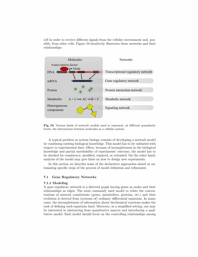
cell in order to receive different signals from the cellular environment and, pos-sibly, from other cells. Figure 10 intuitively illustrates these networks and theirrelationships.

mRNA

Protein

transcription factor

DNAGene

Metabolite

Heterogeneouscomponents

A + C AC B + C

Transcriptional regulatory network

Gene regulatory network

Protein interaction network

Metabolic network

Signaling network

Molecules Networks

Fig. 10. Various kinds of network models used to represent, at different granularitylevels, the interactions between molecules in a cellular system.

A typical problem in system biology consists of developing a network modelby combining existing biological knowledge. This model has to be validated withrespect to experimental data. Often, because of incompleteness in the biologicalknowledge and partial unreliability of experiments’ outcome, the model has tobe checked for consistency, modified, repaired, or extended. On the other hand,analysis of the model may give hints on how to design new experiments.

In this section we describe some of the declarative approaches aimed at au-tomating specific steps of the process of model definition and refinement.

7.1 Gene Regulatory Networks

7.1.1 ModelingA gene regulatory network is a directed graph having genes as nodes and theirrelationships as edges. The most commonly used model to relate the concen-trations of network constituents (genes, metabolites, proteins, etc.) and theirevolution is derived from (systems of) ordinary differential equations. In manycases, the incompleteness of information about biochemical reactions makes thetask of defining such equations hard. Moreover, in a simplified setting, one maybe interested in abstracting from quantitative aspects and introducing a qual-itative model. Such model should focus on the controlling relationships among

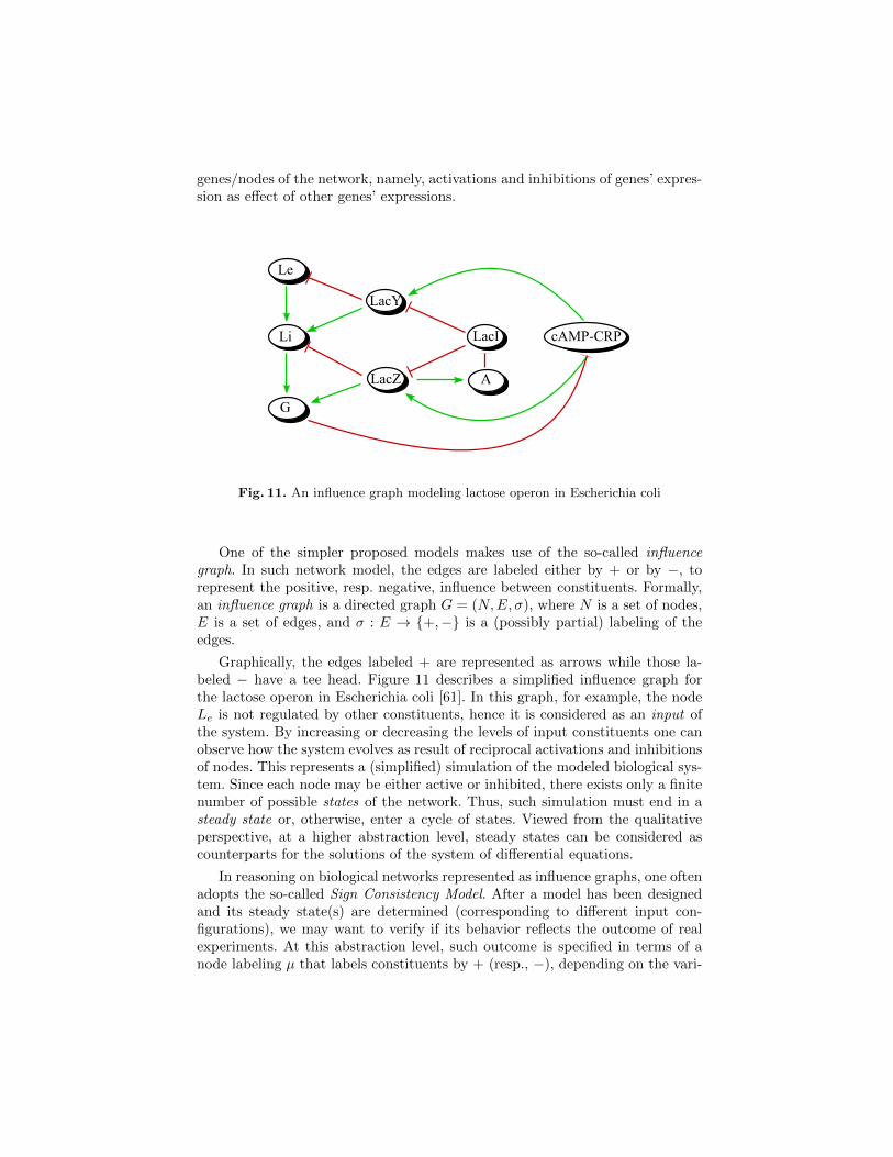
genes/nodes of the network, namely, activations and inhibitions of genes’ expres-sion as effect of other genes’ expressions.

Le

Li

G

LacY

LacZ A

LacI cAMP-CRP

Fig. 11. An influence graph modeling lactose operon in Escherichia coli

One of the simpler proposed models makes use of the so-called influencegraph. In such network model, the edges are labeled either by + or by −, torepresent the positive, resp. negative, influence between constituents. Formally,an influence graph is a directed graph G = (N,E, σ), where N is a set of nodes,E is a set of edges, and σ : E → {+,−} is a (possibly partial) labeling of theedges.

Graphically, the edges labeled + are represented as arrows while those la-beled − have a tee head. Figure 11 describes a simplified influence graph forthe lactose operon in Escherichia coli [61]. In this graph, for example, the nodeLe is not regulated by other constituents, hence it is considered as an input ofthe system. By increasing or decreasing the levels of input constituents one canobserve how the system evolves as result of reciprocal activations and inhibitionsof nodes. This represents a (simplified) simulation of the modeled biological sys-tem. Since each node may be either active or inhibited, there exists only a finitenumber of possible states of the network. Thus, such simulation must end in asteady state or, otherwise, enter a cycle of states. Viewed from the qualitativeperspective, at a higher abstraction level, steady states can be considered ascounterparts for the solutions of the system of differential equations.

In reasoning on biological networks represented as influence graphs, one oftenadopts the so-called Sign Consistency Model. After a model has been designedand its steady state(s) are determined (corresponding to different input con-figurations), we may want to verify if its behavior reflects the outcome of realexperiments. At this abstraction level, such outcome is specified in terms of anode labeling µ that labels constituents by + (resp., −), depending on the vari-

ations of their concentrations, as exhibited by experimental data. Consistencyof the model with respect of the experimental data is formalized a follows.

Let G = (N,E, σ) be an influence graph and µ : N → {+,−} a (partial)node labeling. Then, G and µ are consistent if there are extensions σ′ of σand µ′ of µ such that, for each non-input node n ∈ N , there is an edge e =(m,n) ∈ E such that σ′(e) ◦ µ′(m) = µ′(n), where the usual rule for signs,namely + ◦+ = − ◦ − = + and − ◦+ = + ◦ − = −, is adopted.

Even in this simplified setting, the problem of establishing consistency of amodel w.r.t. a data set is not trivial. In [114], for instance, it is shown that inpresence of incomplete information the decision problem is NP-hard.

In case inconsistency is detected, this can be caused by missing or inaccu-rate knowledge involved in the design of the network and by the presence ofpartially unreliable data. In such a situation, one may ask whether it is possibleto reconcile model and data. A possibility consists in applying some changes inthe network model or in the data (or both). Changing the data is an attemptin singling out those portions of the experimental outcome to be considered asunreliable. A modification of the network should yield a more refined biologicalmodel. Finding a set of such repairing operations consists in solving the re-pair problem. This is usually solved with respect to a collection of experimentalprofiles—observations or experimental evidences—represented as a collection ofdifferent node labeling.

Considering a set of experimental profiles, a typical repair operation consistsof: 1) introducing a new edge in the network; 2) flipping the label of an edge;3) considering a node to be an input node in all experimental profiles; 4) con-sidering a node to be an input node in a specific profile; 5) flipping the label fora node in a specific profile. 1) and 2) correct incompleteness and inaccuracy ofthe model; 3) indicates that for that node some form of regulation is missing inthe model; 4) and 5) revise the experimental observations.

We are interested in applying a minimal number of repair operations. Thuswe are looking for repairs that are minimal with respect to some criteria. Twopossibilities explored in literature [59], are subset-minimality and cardinality-minimality. As noted in [59], both choices are not computationally trivial, sinceevaluating subset-minimality and cardinality-minimality involves solving prob-lems that are, in general, in ΣP

2 and in ∆P2 , respectively.

It is possible that many repairs exist for reconciling the same inconsistencybetween a network and a set of profiles. We may be interested in detecting thoseparts in the edge/node labeling that are common to all these solutions. In otherwords, we are interested in determining the consequences of each minimal repair.This consists of solving the prediction problem.

7.1.2 ASP EncodingThe following encoding is inspired from [61, 59] but it avoids the use of disjunc-tive heads and it deals with consistency detection and with a simple notion ofrepairing.

The program aims to compute the predicates label vertex and label edges

(although typically edges are already labeled). The input of the problem is giventhrough a set of facts of the following kind: vertex(Vertex Name), edges(FromVertex, To Vertex), input(vertex Name)–for input vertices, and a set ofobservation for nodes and edges of the form observed(Vertex name, Sign)

(for nodes) and observed(From Vertex, To Vertex, Sign) (for edges), whereSign is either plus or minus.

% domain predicates

(1) sign(minus). sign(plus).

(2) opposite(minus,plus). opposite(plus,minus).

% Non deterministic labels for nodes and edges

(3) 1 {label_vertex(V,S): sign(S)} 1 :- vertex(V).

(4) 1 {label_edge(U,V,S): sign(S)} 1 :- edge(U,V).

% choice for reversing an edge

(5) {wrong(U,V)} :- edge(U,V).

% labeling nodes consistent with observation

(6) label_vertex(V,S) :- observed(V,S).

% labeling edges consistent with observation, if possible

(7) label_edge(U,V,S) :- wrong(U,V), observed(U,V,T), opposite(S,T).

(8) label_edge(U,V,S) :- not wrong(U,V), observed(U,V,S).

% Rules of signs

(9) receive(V, plus) :- edge(U,V), sign(S),

label_edge(U, V, S), label_vertex(U, S).

(10) receive(V, minus) :- edge(U,V), opposite(S,T),

label_edge(U, V, S), label_vertex(U, T).

% All vertices (but inputs) must be labeled in justified way

(11) :- label_vertex(V, S), not receive(V, S), not input(V).

% Minimize edge reversing to guarantee consistency

(12) edges_reversed(N) :- N = #count{ wrong(U,V) }.

(13) #minimize [edges_reversed(N)=N].

After defining the domain predicate sign in line (1), and the predicate oppo-site between signs, the mutual exclusion between plus and minus for vertices andedges is stated in lines (3) and (4). The choice for the predicate wrong stating,intuitively, that an edge should be reversed is added in line (5). The labeling weare looking for should be consistent with known observations. In particular, nodelabeling is required to be consistent in line (6) and the edge labeling is consistentif the edge is not wrong, otherwise the complementary value is chosen (lines (7)and (8)). Rules of signs propagation are stated in lines (9) and (10), using theauxiliary predicate receive. Then, in line (11) it is stated that the labeling ofthe non-input vertex must be justified by the predicate receive, namely by therule of signs. Lines (12) and (13) are inserted for looking for the answer set witha minimum number of wrong edges. If edges reversed(0) is in the result, thenthe network is already consistent.

7.2 Metabolic Networks

7.2.1 ModelingLarge amounts of data are made available through experiments, making possiblethe study of the dynamic metabolic behavior of living cells (or systems of cells)in response to perturbations and stimuli coming from their surrounding environ-ment. This is usually done by analyzing metabolic networks. In such networks,the nodes represent the metabolites while the edges represent the reactions. Ametabolic network describes a collection of metabolite components together witha functional readout of the cellular state. The modeling and the reconstruction ofbiochemical reaction pathways/networks are far from being easy tasks, becauseof the complexity of the molecules and the reactions that may take place. Thisfact calls for sophisticated and refined computational techniques for reconstruct-ing and simulating metabolic networks.

Several formal techniques and approaches have been adopted to model andreason about metabolic networks. Among them, we find Petri nets, Flux balanceanalysis, and Process calculi (see [20], and the references therein, for furtherdetails).

In the rest of this section we describe a qualitative approach based on ASPto study this class of problems. We rely on the notion of metabolic networkborrowed from [89, 97, 25]. Intuitively speaking, a metabolic network modelssituations where a reaction can only occur if all of its substrates are availableas nutrients or can be produced by other reactions. Starting from some initiallygiven nutrients, called seeds, the network is expanded by adding all of the enabledreactions together with their products. Such a process iterates until no furtherreactions can occur. The set of metabolites in the expanded resulting networkis called the scope of the given seeds. It represents all the metabolites that canbe, potentially, synthesized from the seeds by the given network.

We adopt the following definition: a metabolic network is a directed bipartitegraph G = (R ∪M,E) where R and M are sets of nodes representing reactionsand metabolites, respectively, and E ⊆ (R×M) ∪ (M ×R).

Given an edge (m, r) ∈ E, the metabolite m ∈ M is called reactant of thereaction r ∈ R. Similarly, for an edge (r,m) ∈ E, the metabolite m ∈ M iscalled product of the reaction r. We say that a reaction r is reachable from a setof metabolites S if S contains all the reactants of r. Moreover, we say that ametabolite m is reachable from a set of metabolites S if either m ∈ S or m is aproduct of some reaction r reachable from S. We define the scope of a set S ofmetabolites in the network G (briefly, ΣG(S)) to be the set of metabolites thatare (transitively) reachable from S.

The authors of [97, 25] propose ASP-based solutions for two specific reasoningtasks on metabolic networks: metabolic network completion and inverse scopeproblem.

The metabolic network completion problem can be stated as follows. Let usconsider a metabolic network G = (R ∪M,E), two sets S, T ⊆ M of seed andtarget metabolites, and a reference metabolic network (R′∪M ′, E′). We wish to

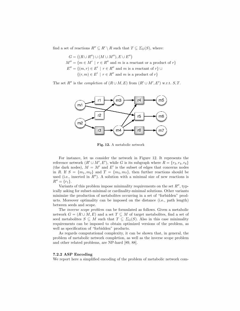
find a set of reactions R′′ ⊆ R′ \R such that T ⊆ ΣG(S), where:

G =((R ∪R′′) ∪ (M ∪M ′′), E ∪ E′′

)M ′′ = {m ∈M ′ | r ∈ R′′ and m is a reactant or a product of r}E′′ = {(m, r) ∈ E′ | r ∈ R′′ and m is a reactant of r} ∪

{(r,m) ∈ E′ | r ∈ R′′ and m is a product of r}

The set R′′ is the completion of (R ∪M,E) from (R′ ∪M ′, E′) w.r.t. S, T .

Fig. 12. A metabolic network

For instance, let us consider the network in Figure 12. It represents thereference network (R′ ∪M ′, E′), while G is its subgraph where R = {r3, r4, r6}(the dark nodes), M = M ′ and E′ is the subset of edges that concerns nodesin R. If S = {m1,m2} and T = {m5,m7}, then further reactions should beused (i.e., inserted in R′′). A solution with a minimal size of new reactions isR′′ = {r1}.

Variants of this problem impose minimality requirements on the set R′′, typ-ically asking for subset-minimal or cardinality-minimal solutions. Other variantsminimize the production of metabolites occurring in a set of “forbidden” prod-ucts. Moreover optimality can be imposed on the distance (i.e., path length)between seeds and scope.

The inverse scope problem can be formulated as follows. Given a metabolicnetwork G = (R ∪M,E) and a set T ⊆ M of target metabolites, find a set ofseed metabolites S ⊆ M such that T ⊆ ΣG(S). Also in this case minimalityrequirements can be imposed to obtain optimized versions of the problem, aswell as specification of “forbidden” products.

As regards computational complexity, it can be shown that, in general, theproblem of metabolic network completion, as well as the inverse scope problemand other related problems, are NP-hard [89, 88].

7.2.2 ASP EncodingWe report here a simplified encoding of the problem of metabolic network com-

pletion. The interested reader can refer to [97] for a description of variants ofthis encoding as well as for the ASP formulation of the inverse scope problem.

The instance of the problem is described by the specification of two networks.This is done using facts of the forms:

• draft(Net) to identify the network named Net as the network G.

• reaction(R,Net) states that the reaction node is in G;

• Other reactions of G′ are defined by reaction(R,a) (a stands for “all”;w.l.o.g. let us assume that the network name Net is not a, and that it isdifferent from the symbol x, as well).

• Edges are represented by facts of the form reactant(M,R) and product(M,R)

to specify the topology of the network.

• seed(S) and target(T) specify seeds and targets.

For instance, considering again the network in Figure 12, one can state draft(d)to identify G, along with the facts

reaction(r1, a). reaction(r2, a). reaction(r3, d). ...

The graph is given by facts of the form:

reactant(m1, r1). reactant(m2, r2). ...

product(m3, r1). product(m3, r2). ...

Finally, seeds and target are defined as

seed(m1). seed(m2). target(m5). target(m7).

The following code implements the solution to the the problem of metabolicnetwork completion.

%%% Type of reaction. d: graph G, a: all, x: reactions added

(1) type(Net) :- draft(Net).

(2) type(a). type(x).

%%% Extended graph.

(3) reaction(R,x) :- reaction(R,Net), draft(Net).

(4) { reaction(R,x) } :- reaction(R,a).

%%% reachability predicate

(5) scope(M, T) :- seed(M), type(T).

(6) scope(M, T) :- type(T), product(M,R), reaction(R,T),

scope(M2,T) : reactant(M2,R).

(7) :- target(M), not scope(M,x).

%%% new reactions and their minimization

(8) new(R) :- reaction(R,x), draft(Net), not reaction(R,Net).

(9) reactions(S) :- S = #count{ new(R) }.

(10) #minimize[reactions(S)=S].

In the above code, lines (1)–(2) define the three types of reactions, d stands forthe network G, a stands for the reference network, and x will denote the reactionsof the intermediate network G′′ we are looking for. Lines (3)–(4) define non-deterministically which reaction can be considered by the intermediate networkG′′. All reactions of G are included, while those in G′ \G can be considered or

not. Lines (5) and (6) define the reachability relation. In particular, let us observethe use of the conditional literal scope(M2,T) : reactant(M2,R) in the body ofthe rule of line (6). It is a shorthand for scope(m1, T ), . . . , scope(mn, T ) wherem1, . . . ,mn are all the metabolites that are reactants of the reaction R active inthe network identified by T . This kind of syntactic extension to ASP is replacedby the proper list of usual literals by the grounding stage. The constraint inline (7) imposes that all targets must be obtained in the extended network.Finally, lines (8)–(10) ask for a cardinality-minimal set of new reactions.

7.3 Related work

It is practically impossible to compile here a comprehensive bibliography onSystems Biology. We refer the reader to [44], which provides a general overviewof the field and an extensive bibliography, and to [20] for a network-orientedperspective. Let us focus on the declarative approaches developed in the subfieldsof Systems Biology treated in this chapter.

In this section, we described the approach relying on the notion of InfluenceGraph and the Sign Consistency Model for gene regulatory networks. Othermethods have been studied; for instance, [28, 27, 19, 26, 58] adopt, and in somecases extend, the logical formalism introduced in [104, 105, 106]. Notions of net-work, such as regulatory graphs and interaction graphs [54], are defined similarlyto influence graphs, but by admitting numerical labeling or activation/inhibitionthresholds. Implementations have also been developed, such as SysBiOX [27] andPint [58], exploiting computational logic solvers, mainly based on SAT, ASP,or CSP.

Boolean networks have been also used, for instance in [71], to declarativelytackle the learning problem for biological network models. The proposal ex-ploits an ASP-solver as reasoning engine. Similarly, [54] relies on ASP to modeland reason about protein interactions, while [93] integrates numerical weightsin Boolean networks in order to introduce a notion of preference among solu-tions. Another extension of Boolean networks is used in [55, 56] to develop anASP-based system to model regulatory networks with meta-interactions. Theimplementations of a collection of deductive tasks for reasoning on biologicalnetworks, developed by the authors of [71, 45, 59, 61] (including those presentedin this section), are described in [60].

The use of Action Description Languages to solve different computationallyhard problems in Systems Biology has been explored in [112, 111, 6, 7, 113]. Theauthors also realized a tool, named BioSigNet-RR, exploiting such ideas. Similarapproaches to signaling, metabolic, and regulation networks have been proposedin [46, 47], among others, by introducing the ADL CTAID and the system BioC.

In [16] a software environment for modeling biochemical systems (BIOCHAM)has been described. It allows the analysis and simulation of Boolean, kinetic, andstochastic models and the formalization of biological properties in temporal logic.Parts of the tool are implemented in logic programming.

8 Conclusions

This chapter reviews some classical problems that arise in Bioinformatics, namelyPhylogenetics, Haplotype, RNA secondary structure prediction, protein struc-ture prediction, and systems biology. The chapter shows how logic programmingcan be employed to model these problems by describing the properties of the sys-tem, rather than the process of computing the problem’s solutions. The problemshave been modeled by means of Answer Set Programming, a logic programminglanguage that allows concise and versatile programming style. The reader isguided into the modeling process and the intuitive encoding into ASP. The rela-tively short encodings are fully functional and they can be tested in conjunctionwith input reported in the Appendix.

Acknowledgments. We would like to thank the colleagues that helped us inour research in Bioinformatics: Federico Fogolari, Federico Campeotto, PietroCozzini, and Ferdinando Fioretto, and also the friends that has helped us inorganizing the workshops on constraint based methods for bioinformatics, and inparticular Sebastian Will, Rolf Backofen, and Francois Fages. Finally, we thankthe organizers of the ACP school 2012: Krzysztof Apt, Witold Charatonik, andLeszek Pacholski that gave us the stimulus for organizing this material.

References

[1] Thematic series of AMB on constraints and bioinformatics, 2012.[2] C. B. Anfinsen. Principles that govern the folding of protein chains. Science,

181:223–230, 1973.[3] R. Backofen. The protein structure prediction problem: A constraint optimiza-

tion approach using a new lower bound. Constraints, 6(2–3):223–255, 2001.[4] R. Backofen and S. Will. A constraint-based approach to fast and exact structure

prediction in three-dimensional protein models. Constraints, 11(1):5–30, 2006.[5] P. O. Barahona P., Krippahl L. Bioinformatics: A challenge to constraint pro-

gramming. Hybrid Optimization, 45:463–487, 2011.[6] C. Baral, K. Chancellor, N. Tran, and N. Tran. Representing and reasoning about

signal networks: an illustration using NFκB dependent signaling pathways. InCSB, pages 623–628. IEEE Computer Society, 2003.

[7] C. Baral, K. Chancellor, N. Tran, N. Tran, A. M. Joy, and M. E. Berens. Aknowledge based approach for representing and reasoning about signaling net-works. In ISMB/ECCB (Supplement of Bioinformatics), pages 15–22, 2004.

[8] M. Bauer, G. W. Klau, and K. Reinert. RNA pseudoknot prediction in energy-based models. BMC Bioinformatics, 8, 2007.

[9] M. Bavarian and V. Dahl. Constraint based methods for biological sequenceanalysis. Journal of Universal Computer Science, 12(11):1500–1520, nov 2006.

[10] D. Brooks, E. Erdem, S. Erdogan, J. Minett, and D. Ringe. Inferring phylo-genetic trees using answer set programming. Journal of Automated Reasoning,39(4):471–511, 2007.

[11] D. Brooks, E. Erdem, J. Minett, and D. Ringe. Character-based cladistics andanswer set programming. In Practical Aspects of Declarative Languages, pages37–51. Springer Verlag, 2005.

[12] D. G. Brown and I. M. Harrower. Integer programming approaches to haplo-type inference by pure parsimony. IEEE/ACM Transactions on ComputationalBiology and Bioinformatics, 3(2):141–154, 2006.

[13] D. Cakmak. Reconstructing weighted phylogenetic trees and weighted phyloge-netic networks using answer set programming. Master’s thesis, Sabanc Univer-sity, 2010.

[14] D. Cakmak, E. Erdem, and H. Erdogan. Computing weighted solutions in answerset programming. In Logic Programming and Nonmonotonic Reasoning, pages416–422. Springer Verlag, 2009.

[15] D. Cakmak, H. Erdogan, and E. Erdem. Computing weighted solutions in ASP:Representation-based method vs. search-based method. In Proc. of RCRA Work-shop on Experimental Evaluation of Algorithms for Solving Problems with Com-binatorial Explosion, 2010.

[16] L. Calzone, F. Fages, and S. Soliman. Biocham: an environment for model-ing biological systems and formalizing experimental knowledge. Bioinformatics,22(14):1805–1807, 2006.

[17] F. Campeotto, A. Dal Palu, A. Dovier, F. Fioretto, and E. Pontelli. A filteringtechnique for fragment assembly- based proteins loop modeling with constraints.In M. Milano, editor, CP, volume 7514 of Lecture Notes in Computer Science,pages 850–866. Springer, 2012.

[18] D. Catanzaro and M. Labbe. The pure parsimony haplotyping problem: overviewand computational advances. International Transactions in Operational Re-search, 16(5):561–584, 2009.

[19] C. Chaouiya, E. Remy, B. Mosse, and D. Thieffry. Qualitative analysis of reg-ulatory graphs: A computational tool based on a discrete formal framework. InL. Benvenuti, A. D. Santis, and L. Farina, editors, POSTA, volume 294 of LectureNotes in Control and Information Sciences, pages 119–126. Springer, 2003.

[20] L. Chen, R.-S. Wang, and X.-S. Zhang. Biomolecular Networks: Methods andApplications in Systems Biology. John Wiley & Sons, 2009.

[21] B. Chisham, B. Wright, T. Le, T. Son, and E. Pontelli. CDAO-Store: Ontology-driven Data Integration for Phylogenetic Analysis. BMC Bioinformatics, 12:98,2011.

[22] A. G. Clark. Inference of haplotypes from PCR amplified samples of diploidpopulations. Molecular Biology and Evolution, 7(2):111–122, 1990.

[23] P. Clote and R. Backofen. Computational Molecular Biology: An Introduction.John Wiley & Sons, 2001.

[24] E. Coban, E. Erdem, and F. Ture. Comparing ASP, CP, ILP on some challengingproblems. In The 2nd International Workshop on Logic and Search – LaSh08,2008.

[25] G. Collet, D. Eveillard, M. Gebser, S. Prigent, T. Schaub, A. Siegel, andS. Thiele. Extending the metabolic network of EctocarpusSiliculosus using an-swer set programming. In P. Cabalar and T. Son, editors, Logic Programmingand Nonmonotonic Reasoning, volume 8148 of Lecture Notes in Computer Sci-ence, pages 245–256. Springer Berlin Heidelberg, 2013.

[26] F. Corblin, E. Fanchon, and L. Trilling. Applications of a formal approach todecipher discrete genetic networks. BMC Bioinformatics, 11:385, 2010.

[27] F. Corblin, E. Fanchon, L. Trilling, C. Chaouiya, and D. Thieffry. Automatic in-ference of regulatory and dynamical properties from incomplete gene interactionand expression data. In M. A. Lones, S. L. Smith, S. A. Teichmann, F. Naef,J. A. Walker, and M. Trefzer, editors, IPCAT, volume 7223 of Lecture Notes inComputer Science, pages 25–30. Springer, 2012.

[28] F. Corblin, S. Tripodi, E. Fanchon, D. Ropers, and L. Trilling. A declara-tive constraint-based method for analyzing discrete genetic regulatory networks.Biosystems, 98(2):91–104, 2009.

[29] P. Crescenzi, D. Goldman, C. Papadimitrou, A. Piccolboni, and M. Yannakakis.On the complexity of protein folding. In Proc. of STOC, pages 597–603, 1998.

[30] F. Crick. Central dogma of molecular biology. Nature, 227:561–3, 1970.[31] A. Dal Palu, A. Dovier, F. Fages, and S. Will. Constraint based methods for

bioinformatics. In PART VI of Trends in Constraint Programming, pages 125–146. Hermes Science, 2007.

[32] A. Dal Palu, A. Dovier, and F. Fogolari. Constraint logic programming approachto protein structure prediction. BMC Bioinformatics, 5:186, 2004.

[33] A. Dal Palu, A. Dovier, F. Fogolari, and E. Pontelli. CLP-based protein fragmentassembly. TPLP, 10(4-6):709–724, 2010.

[34] A. Dal Palu, A. Dovier, F. Fogolari, and E. Pontelli. Protein Structure Anal-ysis with Constraint Programming. In P. Cozzini, G. Kellogg, D. Rotella, andA. Martinez, editors, Computational Approaches to Nuclear Receptors, chapter 3,pages 40–59. The Royal Society of Chemistry, 2012.

[35] A. Dal Palu, A. Dovier, and E. Pontelli. A constraint solver for discrete lattices,its parallelization, and application to protein structure prediction. Softw., Pract.Exper., 37(13):1405–1449, 2007.

[36] A. Dal Palu, A. Dovier, and S. Will. Introduction to the special issue on bioin-formatics and constraints. Constraints, 13(1-2):1–2, June 2008.

[37] A. Dal Palu, M. Mohl, and S. Will. A propagator for maximum weight stringalignment with arbitrary pairwise dependencies. In Proceedings of the 16th inter-national conference on Principles and practice of constraint programming, CP’10,pages 167–175, Berlin, Heidelberg, 2010. Springer-Verlag.

[38] W. Day. Computationally difficult parsimony problems in phylogenetic system-atics. Journal of Theoretical Biology, 103(3):429–438, 1983.

[39] W. Day and D. Sankoff. Computational complexity of inferring phylogenies bycompatibility. Systematic Zoology, 35(2):224–229, 1986.

[40] L. Di Gaspero and A. Roli. Stochastic local search for large-scale instances of thehaplotype inference problem by pure parsimony. J. Algorithms, 63(1-3):55–69,2008.

[41] K. A. Dill. Dominant forces in protein folding. Biochemistry, 29:7133–7155,1990.

[42] A. Dobson. Lexicostatistical grouping. Anthropological Linguistics, 11:216–221,1969.

[43] A. Dovier, A. Formisano, and E. Pontelli. An empirical study of constraint logicprogramming and answer set programming solutions of combinatorial problems.J. Exp. Theor. Artif. Intell., 21(2):79–121, 2009.

[44] W. Dubitzky, O. Wolkenhauer, K.-H. Cho, and H. Yokota. Encyclopedia ofSystems Biology. Springer, 2013.

[45] M. Durzinsky, W. Marwan, M. Ostrowski, T. Schaub, and A. Wagler. Automaticnetwork reconstruction using ASP. TPLP, 11(4-5):749–766, 2011.

[46] S. Dworschak, S. Grell, V. J. Nikiforova, T. Schaub, and J. Selbig. Modeling bi-ological networks by action languages via answer set programming. Constraints,13(1-2):21–65, 2008.

[47] S. Dworschak, T. Grote, A. Konig, T. Schaub, and P. Veber. The system BioCfor reasoning about biological models in action language C. In ICTAI (1), pages11–18. IEEE Computer Society, 2008.

[48] E. Erdem. Applications of answer set programming in phylogenetic systemat-ics. In M. Balduccini and T. C. Son, editors, Logic Programming, KnowledgeRepresentation, and Nonmonotonic Reasoning, volume 6565 of Lecture Notes inComputer Science, pages 415–431. Springer, 2011.

[49] E. Erdem, O. Erdem, and F. Ture. HAPLO-ASP: Haplotype inference usinganswer set programming. In E. Erdem, F. Lin, and T. Schaub, editors, LogicProgramming and Nonmonotonic Reasoning, 10th International Conference, LP-NMR 2009, Potsdam, Germany, September 14-18, 2009. Proceedings, volume5753 of Lecture Notes in Computer Science, pages 573–578. Springer, 2009.

[50] E. Erdem, V. Lifschitz, L. Nakhleh, and D. Ringe. Reconstructing the evo-lutionary history of Indo-European languages using answer set programming.In Practical Aspects of Declarative Languages, pages 160–176. Springer Verlag,2003.

[51] E. Erdem, V. Lifschitz, and D. Ringe. Temporal phylogenetic networks and logicprogramming. Theory and Practice of Logic Programming, 6(5):539–558, 2006.

[52] E. Erdem and F. Ture. Efficient haplotype inference with answer set program-ming. In D. Fox and C. P. Gomes, editors, Proceedings of the Twenty-Third AAAIConference on Artificial Intelligence, AAAI 2008, Chicago, Illinois, USA, July13-17, 2008, pages 436–441. AAAI Press, 2008.

[53] G. Estabrook. Ancestor-descendant relations and incompatible data: Motivationfor research in discrete mathematics. In Mathematical Hierarchies and Biology,volume 27 of DIMAS Series in Discrete Mathematics, pages 1–28. AmericanMathematical Society, 1997.

[54] T. Fayruzov, M. D. Cock, C. Cornelis, and D. Vermeir. Modeling protein inter-action networks with answer set programming. In BIBM, pages 99–104. IEEEComputer Society, 2009.

[55] T. Fayruzov, J. Janssen, C. Cornelis, D. Vermeir, and M. De Cock. Extendingboolean regulatory network models with answer set programming. In Proceed-ings 2010 IEEE International Conference on Bioinformatics and BiomedicineWorkshops (BIBMW 2010), pages 207–212. IEEE, 2010.

[56] T. Fayruzov, J. Janssen, D. Vermeir, C. Cornelis, and M. D. Cock. Modellinggene and protein regulatory networks with answer set programming. IJDMB,5(2):209–229, 2011.

[57] C. Floudas. Computational methods in protein structure prediction. Biotech-nology and Bioengineering, 97(2):207–213, 2007.

[58] M. Folschette, L. Pauleve, K. Inoue, M. Magnin, and O. Roux. Concretizing theprocess hitting into biological regulatory networks. In D. Gilbert and M. Heiner,editors, CMSB, volume 7605 of Lecture Notes in Computer Science, pages 166–186. Springer, 2012.

[59] M. Gebser, C. Guziolowski, M. Ivanchev, T. Schaub, A. Siegel, S. Thiele, andP. Veber. Repair and prediction (under inconsistency) in large biological net-works with answer set programming. In F. Lin, U. Sattler, and M. Truszczynski,editors, KR. AAAI Press, 2010.

[60] M. Gebser, A. Konig, T. Schaub, S. Thiele, and P. Veber. The BioASP library:ASP solutions for systems biology. In ICTAI (1), pages 383–389. IEEE ComputerSociety, 2010.

[61] M. Gebser, T. Schaub, S. Thiele, and P. Veber. Detecting inconsistencies in largebiological networks with answer set programming. TPLP, 11(2-3):323–360, 2011.

[62] H. Gleason. Counting and calculating for historical reconstruction. Anthropo-logical Linguistics, 1:22–32, 1959.

[63] G. H. Gonnet. Some string matching problems from bioinformatics whichstill need better solutions. Journal of Discrete Algorithms, 2(1):3 – 15, 2004.¡ce:title¿The 9th International Symposium on String Processing and Informa-tion Retrieval¡/ce:title¿.

[64] A. Graca, I. Lynce, J. Marques-Silva, and A. L. Oliveira. Haplotype inferenceby pure parsimony: A survey. Journal of Computational Biology, 17(8):969–992,2010.

[65] A. Graca, J. Marques-Silva, and I. Lynce. Haplotype inference using proposi-tional satisfiability. In R. Bruni, editor, Mathematical Approaches to PolymerSequence Analysis and Related Problems, pages 127–147. Springer, 2011.

[66] T. Gruber. Toward principles for the design of ontologies used for knowedgesharing. International Journal of Human Computer Studies, 43(5-6), 1995.

[67] D. Gusfield. Algorithms on strings, trees, and sequences: computer science andcomputational biology. Cambridge University Press, New York, NY, USA, 1997.

[68] D. Gusfield. Haplotyping as perfect phylogeny: conceptual framework and ef-ficient solutions. In Sixth Annual International Conference on ComputationalBiology, pages 166–175. ACM, 2002.

[69] D. Gusfield. An overview of combinatorial methods for haplotype inference. InIstrail et al. [74], pages 9–25.

[70] D. Gusfield and S. H. Orzack. Haplotype inference. In S. Aluru, editor, Handbookof Computational Molecular Biology, Computer & Information Science, chap-ter 18. Chapman & Hall/CRC, 2005.

[71] C. Guziolowski, S. Videla, F. Eduati, S. Thiele, T. Cokelaer, A. Siegel, andJ. Saez-Rodriguez. Exhaustively characterizing feasible logic models of a signal-ing network using answer set programming. Bioinformatics, 29(18):2320–2326,2013.

[72] B. V. Halldorsson, V. Bafna, N. Edwards, R. Lippert, S. Yooseph, and S. Istrail.A survey of computational methods for determining haplotypes. In Istrail et al.[74], pages 26–47.

[73] International Human Genome Sequencing Consortium. Finishing the euchro-matic sequence of the human genome. Nature, 431:931–45, 2004.

[74] S. Istrail, M. S. Waterman, and A. G. Clark, editors. Computational Methods forSNPs and Haplotype Inference, DIMACS/RECOMB Satellite Workshop, Piscat-away, NJ, USA, November 21-22, 2002, Revised Papers, volume 2983 of LectureNotes in Computer Science. Springer, 2004.

[75] G. Jin, L. Nakhleh, S. Snir, and T. Tuller. Inferring phylogenetic networks bythe maximum parsimony criterion: a case study. Mol Biol Evol, 24(1):324–337,2007.

[76] M. JS. The equilibrium partition function and base pair binding probabilitiesfor RNA secondary structure. Biopolymers, 29(6–7):1105–19, 1990.

[77] G. Lancia, M. C. Pinotti, and R. Rizzi. Haplotyping populations by pure parsi-mony: Complexity of exact and approximation algorithms. INFORMS Journalon Computing, 16(4):348–359, 2004.

[78] T. Le, H. Nguyen, E. Pontelli, and T. Son. ASP at Work: An ASP Implemen-tation of PhyloWS. In International Conference on Logic Programming, pages359–369, 2012.

[79] W. Le Quesne. A Method of Selection of Characters in Numerical Taxonomy.Syst. Zool., 18:201–205, 1969.

[80] W. Le Quesne. Further Studies Based on the Uniquely Derived Character Con-cept. Syst. Zool., 21:281–288, 1972.

[81] A. Lesk. Introduction to Bioinformatics. Oxford University Press, 2008.[82] C. Letondal. A web interface generator for molecular biology programs in unix.

Bioinformatics, 17(1):73–82, 2001.[83] D. Liberles and M. Wayne. Tracking adaptive evolutionary events in genomic

sequences. Genome Biol., 3(6), 2002.[84] R. Lyngso and C. Pedersen. RNA pseudoknot prediction in energy-based models.

J Computational Biology, 7(3-4):409–427, 2000.[85] E. Mayr. Systematics and the Origin of Species. Dover Publications, 1964.[86] L. Nakhleh, T. Warnow, C. Linder, and K. St John. Reconstructing reticulate

evolution in species-theory and practice. Journal of Computational Biology,12(6):796–811, 2005.

[87] A. Neumaier. Molecular modeling of proteins and mathematical prediction ofprotein structure. SIAM Review, 39:407–460, 1997.

[88] Z. Nikoloski, S. Grimbs, P. May, and J. Selbig. Metabolic networks are NP-hardto reconstruct. Journal of Theoretical Biology, 254(4):807–816, 2008.

[89] Z. Nikoloski, S. Grimbs, J. Selbig, and O. Ebenhoh. Hardness and approxima-bility of the inverse scope problem. In K. A. Crandall and J. Lagergren, edi-tors, WABI, volume 5251 of Lecture Notes in Computer Science, pages 99–112.Springer, 2008.

[90] J. A. Nussinov R. Fast algorithm for predicting the secondary structure of single-stranded RNA. Proc Natl Acad Sci USA, 77(11):6309–6313, 1980.

[91] Y. Pan, E. Pontelli, and T. Son. BSIS: An Experiment in Automating Bioinfor-matics Tasks Through Intelligent Work ow Construction. In Semantic e-Science,pages 189–238. Springer Verlag, 2010.

[92] F. Prosdocimi, B. Chisham, E. Pontelli, J. Thompson, and A. Stoltzfus. Ini-tial Implementation of a Comparative Data Analysis Ontology. EvolutionaryBioinformatics, 5:47–66, 2009.

[93] O. Ray, T. Soh, and K. Inoue. Analyzing pathways using ASP-based approaches.In K. Horimoto, M. Nakatsui, and N. Popov, editors, ANB, volume 6479 ofLecture Notes in Computer Science, pages 167–183. Springer, 2010.

[94] D. Ringe, T.Warnow, and A. Taylor. Indo-European and computational cladis-tics. Transactions of the Philological Society, 100(1):59–129, 2002.

[95] R. Rossnes, I. Eidhammer, and D. Liberles. Phylogenetic reconstruction of an-cestral character states for gene expression and mRNA splicing data. BMCBioinformatics, 6(1):127, 2007.

[96] D. Sankoff. Simultaneous solution of the RNA folding, alignment and protose-quence problems. SIAM Journal on Applied Mathematics, 45(5):810–825, 1985.

[97] T. Schaub and S. Thiele. Metabolic network expansion with answer set program-ming. In P. M. Hill and D. S. Warren, editors, ICLP, volume 5649 of LectureNotes in Computer Science, pages 312–326. Springer, 2009.

[98] A. SF, G. W, M. W, M. EW, and L. DJ. Basic local alignment search tool. JMol Biol, 215(3):403–410, 1990.

[99] R. Sharan, B. V. Halldorsson, and S. Istrail. Islands of tractability for par-simony haplotyping. IEEE/ACM Transactions on Computational Biology andBioinformatics, 3(3):303–311, 2006.

[100] T. Son, E. Pontelli, and T. Le. Two Applications of the ASP-Prolog System:Decomposable Programs and Multi-context Systems. In Practical Aspects ofDeclarative Languages. Springer Verlag, 2013.

[101] E. Stone and A. Sidow. Physicochemical constraint violation by missense substi-tutions mediates impairment of protein function and disease severity. GenomeRes., 15(7):978–986, 2005.

[102] A. Taylor, T. Warnow, and D. Ringe. Character-based reconstruction of a lin-guistic cladogram. In J. Smith and D. Bentley, editors, Historical Linguistics,volume 1, pages 393–408. Benjamins, 2000.

[103] S. Thiele. Modeling Biological Systems With Answer Set Programming. Doctorrerum naturalium thesis, Universitat Polsdam, 2012.

[104] R. Thomas. Regulatory networks seen as asynchronous automata: A logicaldescription. Journal of Theoretical Biology, 153(1):1–23, 1991.

[105] R. Thomas and M. Kaufman. Multistationarity, the basis of cell differentiationand memory. I. structural conditions of multistationarity and other nontrivialbehavior. Chaos: An Interdisciplinary Journal of Nonlinear Science, 11(1):170–179, 2001.

[106] R. Thomas, D. Thieffry, and M. Kaufman. Dynamical behaviour of biologi-cal regulatory networksI. biological role of feedback loops and practical use ofthe concept of the loop-characteristic state. Bulletin of Mathematical Biology,57(2):247–276, 1995.

[107] J. Thorne. Models of protein sequence evolution and their applications. CurrOpin Genet Dev, 10(6):602–605, 2000.

[108] E. Tillier, L. Biro, G. Li, and D. Tillo. Codep: maximizing co-evolutionaryinterdependencies to discover interacting proteins. Proteins, 63(4):822–831, 2006.

[109] E. Tillier and T. Lui. Using multiple interdependency to separate functional fromphylogenetic correlations in protein alignments. Bioinformatics, 19(6):750–755,2003.

[110] L. M. Tinoco I., Uhlenbeck O. Estimation of secondary structure in ribonucleicacids. Nature, 230:363–367, 1971.

[111] N. Tran and C. Baral. Reasoning about non-immediate triggers in biologicalnetworks. Annals of Mathematics and Artificial Intelligence, 51(2-4):267–293,2007.

[112] N. Tran and C. Baral. Hypothesizing about signaling networks. J. Applied Logic,7(3):253–274, 2009.

[113] N. Tran, C. Baral, V. J. Nagaraj, and L. Joshi. Knowledge-based integrativeframework for hypothesis formation in biochemical networks. In B. Ludascherand L. Raschid, editors, DILS, volume 3615 of Lecture Notes in Computer Sci-ence, pages 121–136. Springer, 2005.

[114] P. Veber, M. Le Borgne, A. Siegel, S. Lagarrigue, and O. Radulescu. Complexqualitative models in biology: A new approach. Complexus, 2(3-4):140–151, 2006.

[115] L. Wang and Y. Xu. Haplotype inference by maximum parsimony. Bioinformat-ics, 19(14):1773–1780, 2003.

[116] C. Woese and N. Pace. Probing RNA Structure, Function, and History byComparative Analysis. In The RNA World, pages 91–117. Cold Spring HarborLaboratory Press, 1993.

[117] X. Xia. Bioinformatics and the Cell: Modern Computational Approaches in Ge-nomics, Proteomics and Transcriptomics. Springer, 2007.

[118] Y. Zhao, Y. Xu, Q. Zhang, and G. Chen. An overview of the haplotype problemsand algorithms. Frontiers of Computer Science in China, 1(3):272–282, 2007.

[119] M. Zuker and P. Stiegler. Optimal computer folding of large RNA sequences us-ing thermodynamics and auxiliary information. Nucleic acid research, 9(1):133–148, 1981.

A Instances

For readers’ convenience we report here some instances on which run the ASPencodings presented in the paper (just cut & paste from the pdf—line numbersshould be removed from ASP codes). Expected running time will depend onthe machine of course, but instances are chosen to run in at most a couple ofminutes.

A.1 Phylogenetic Reconstruction

We report here the instance used in Figure 4 and other two simple instances:

– taxa(1..5).

% characters and values on leaves (function f)

f(1,coelom,0). f(2,coelom,0). f(3,coelom,0). f(4,coelom,1). f(5,coelom,1).

f(1,dark,1). f(2,dark,0). f(3,dark,0). f(4,dark,0). f(5,dark,1).

– taxa(1..5).

f(1,a,1). f(2,a,0). f(3,a,0). f(4,a,0). f(5,a,1).

f(1,b,0). f(2,b,1). f(3,b,1). f(4,b,1). f(5,b,0).

f(1,c,1). f(2,c,1). f(3,c,0). f(4,c,0). f(5,c,1).

f(1,d,1). f(2,d,1). f(3,d,1). f(4,d,0). f(5,d,0).

– From http://evolution.berkeley.edu/evolibrary/article/phylogenetics_07

taxa(1..7).

% 1= Sharks and Relatives

f(1,vertebrate,1). f(1,skeleton,0). f(1,fourlimbs,0).

f(1,amnioegg,0). f(1,hair,0). f(1,twopostorbital,0).

% 2 = Ray-finned fishes

f(2,vertebrate,1). f(2,skeleton,1). f(2,fourlimbs,0).

f(2,amnioegg,0). f(2,hair,0). f(2,twopostorbital,0).

% 3 = Amphibians

f(3,vertebrate,1). f(3,skeleton,1). f(3,fourlimbs,1).

f(3,amnioegg,0). f(3,hair,0). f(3,twopostorbital,0).

% 4 = Primates

f(4,vertebrate,1). f(4,skeleton,1). f(4,fourlimbs,1).

f(4,amnioegg,1). f(4,hair,1). f(4,twopostorbital,0).

% 5 = Rodents and rabbits

f(5,vertebrate,1). f(5,skeleton,1). f(5,fourlimbs,1).

f(5,amnioegg,1). f(5,hair,1). f(5,twopostorbital,0).

% 6 = Crocodiles and relatives

f(6,vertebrate,1). f(6,skeleton,1). f(6,fourlimbs,1).

f(6,amnioegg,1). f(6,hair,0). f(6,twopostorbital,1).

% 7 = Dinosaurs and birds

f(7,vertebrate,1). f(7,skeleton,1). f(7,fourlimbs,1).

f(7,amnioegg,1). f(7,hair,0). f(7,twopostorbital,1).

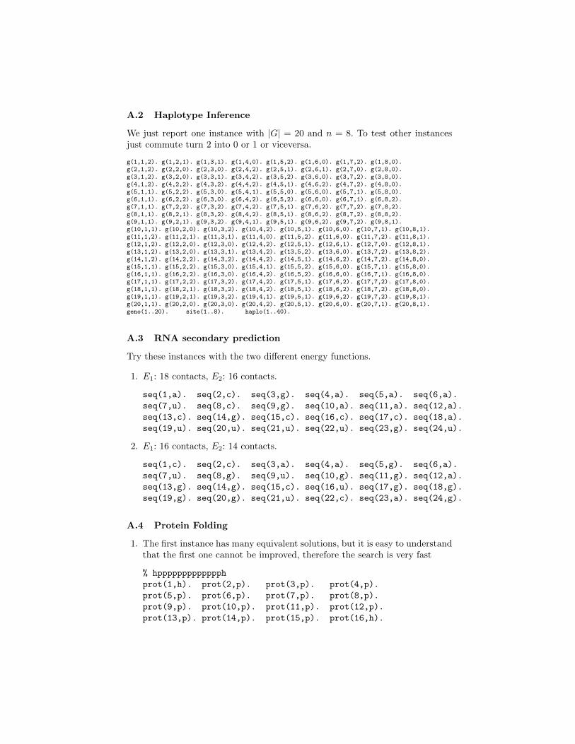
A.2 Haplotype Inference

We just report one instance with |G| = 20 and n = 8. To test other instancesjust commute turn 2 into 0 or 1 or viceversa.

g(1,1,2). g(1,2,1). g(1,3,1). g(1,4,0). g(1,5,2). g(1,6,0). g(1,7,2). g(1,8,0).g(2,1,2). g(2,2,0). g(2,3,0). g(2,4,2). g(2,5,1). g(2,6,1). g(2,7,0). g(2,8,0).g(3,1,2). g(3,2,0). g(3,3,1). g(3,4,2). g(3,5,2). g(3,6,0). g(3,7,2). g(3,8,0).g(4,1,2). g(4,2,2). g(4,3,2). g(4,4,2). g(4,5,1). g(4,6,2). g(4,7,2). g(4,8,0).g(5,1,1). g(5,2,2). g(5,3,0). g(5,4,1). g(5,5,0). g(5,6,0). g(5,7,1). g(5,8,0).g(6,1,1). g(6,2,2). g(6,3,0). g(6,4,2). g(6,5,2). g(6,6,0). g(6,7,1). g(6,8,2).g(7,1,1). g(7,2,2). g(7,3,2). g(7,4,2). g(7,5,1). g(7,6,2). g(7,7,2). g(7,8,2).g(8,1,1). g(8,2,1). g(8,3,2). g(8,4,2). g(8,5,1). g(8,6,2). g(8,7,2). g(8,8,2).g(9,1,1). g(9,2,1). g(9,3,2). g(9,4,1). g(9,5,1). g(9,6,2). g(9,7,2). g(9,8,1).g(10,1,1). g(10,2,0). g(10,3,2). g(10,4,2). g(10,5,1). g(10,6,0). g(10,7,1). g(10,8,1).g(11,1,2). g(11,2,1). g(11,3,1). g(11,4,0). g(11,5,2). g(11,6,0). g(11,7,2). g(11,8,1).g(12,1,2). g(12,2,0). g(12,3,0). g(12,4,2). g(12,5,1). g(12,6,1). g(12,7,0). g(12,8,1).g(13,1,2). g(13,2,0). g(13,3,1). g(13,4,2). g(13,5,2). g(13,6,0). g(13,7,2). g(13,8,2).g(14,1,2). g(14,2,2). g(14,3,2). g(14,4,2). g(14,5,1). g(14,6,2). g(14,7,2). g(14,8,0).g(15,1,1). g(15,2,2). g(15,3,0). g(15,4,1). g(15,5,2). g(15,6,0). g(15,7,1). g(15,8,0).g(16,1,1). g(16,2,2). g(16,3,0). g(16,4,2). g(16,5,2). g(16,6,0). g(16,7,1). g(16,8,0).g(17,1,1). g(17,2,2). g(17,3,2). g(17,4,2). g(17,5,1). g(17,6,2). g(17,7,2). g(17,8,0).g(18,1,1). g(18,2,1). g(18,3,2). g(18,4,2). g(18,5,1). g(18,6,2). g(18,7,2). g(18,8,0).g(19,1,1). g(19,2,1). g(19,3,2). g(19,4,1). g(19,5,1). g(19,6,2). g(19,7,2). g(19,8,1).g(20,1,1). g(20,2,0). g(20,3,0). g(20,4,2). g(20,5,1). g(20,6,0). g(20,7,1). g(20,8,1).geno(1..20). site(1..8). haplo(1..40).

A.3 RNA secondary prediction

Try these instances with the two different energy functions.

1. E1: 18 contacts, E2: 16 contacts.

seq(1,a). seq(2,c). seq(3,g). seq(4,a). seq(5,a). seq(6,a).

seq(7,u). seq(8,c). seq(9,g). seq(10,a). seq(11,a). seq(12,a).

seq(13,c). seq(14,g). seq(15,c). seq(16,c). seq(17,c). seq(18,a).

seq(19,u). seq(20,u). seq(21,u). seq(22,u). seq(23,g). seq(24,u).

2. E1: 16 contacts, E2: 14 contacts.

seq(1,c). seq(2,c). seq(3,a). seq(4,a). seq(5,g). seq(6,a).

seq(7,u). seq(8,g). seq(9,u). seq(10,g). seq(11,g). seq(12,a).

seq(13,g). seq(14,g). seq(15,c). seq(16,u). seq(17,g). seq(18,g).

seq(19,g). seq(20,g). seq(21,u). seq(22,c). seq(23,a). seq(24,g).

A.4 Protein Folding

1. The first instance has many equivalent solutions, but it is easy to understandthat the first one cannot be improved, therefore the search is very fast

% hppppppppppppph

prot(1,h). prot(2,p). prot(3,p). prot(4,p).

prot(5,p). prot(6,p). prot(7,p). prot(8,p).

prot(9,p). prot(10,p). prot(11,p). prot(12,p).

prot(13,p). prot(14,p). prot(15,p). prot(16,h).

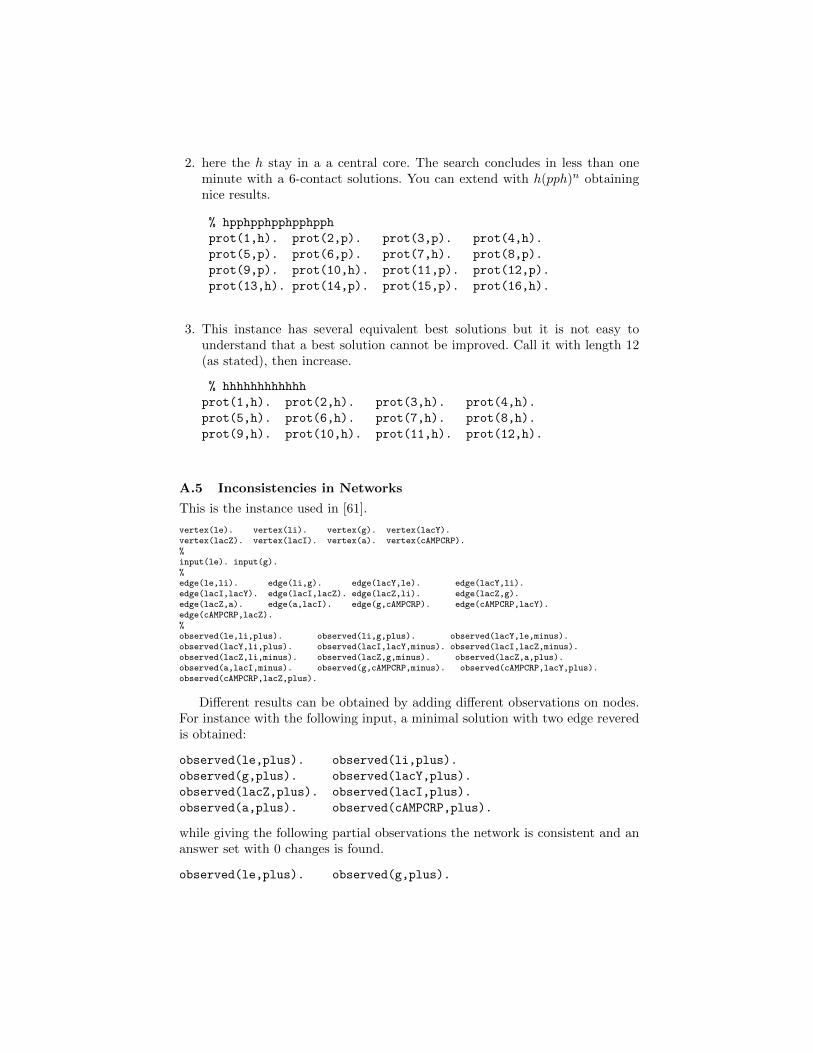
2. here the h stay in a a central core. The search concludes in less than oneminute with a 6-contact solutions. You can extend with h(pph)n obtainingnice results.

% hpphpphpphpphpph

prot(1,h). prot(2,p). prot(3,p). prot(4,h).

prot(5,p). prot(6,p). prot(7,h). prot(8,p).

prot(9,p). prot(10,h). prot(11,p). prot(12,p).

prot(13,h). prot(14,p). prot(15,p). prot(16,h).

3. This instance has several equivalent best solutions but it is not easy tounderstand that a best solution cannot be improved. Call it with length 12(as stated), then increase.

% hhhhhhhhhhhh

prot(1,h). prot(2,h). prot(3,h). prot(4,h).

prot(5,h). prot(6,h). prot(7,h). prot(8,h).

prot(9,h). prot(10,h). prot(11,h). prot(12,h).

A.5 Inconsistencies in Networks

This is the instance used in [61].

vertex(le). vertex(li). vertex(g). vertex(lacY).vertex(lacZ). vertex(lacI). vertex(a). vertex(cAMPCRP).%input(le). input(g).%edge(le,li). edge(li,g). edge(lacY,le). edge(lacY,li).edge(lacI,lacY). edge(lacI,lacZ). edge(lacZ,li). edge(lacZ,g).edge(lacZ,a). edge(a,lacI). edge(g,cAMPCRP). edge(cAMPCRP,lacY).edge(cAMPCRP,lacZ).%observed(le,li,plus). observed(li,g,plus). observed(lacY,le,minus).observed(lacY,li,plus). observed(lacI,lacY,minus). observed(lacI,lacZ,minus).observed(lacZ,li,minus). observed(lacZ,g,minus). observed(lacZ,a,plus).observed(a,lacI,minus). observed(g,cAMPCRP,minus). observed(cAMPCRP,lacY,plus).observed(cAMPCRP,lacZ,plus).

Different results can be obtained by adding different observations on nodes.For instance with the following input, a minimal solution with two edge reveredis obtained:

observed(le,plus). observed(li,plus).

observed(g,plus). observed(lacY,plus).

observed(lacZ,plus). observed(lacI,plus).

observed(a,plus). observed(cAMPCRP,plus).

while giving the following partial observations the network is consistent and ananswer set with 0 changes is found.

observed(le,plus). observed(g,plus).

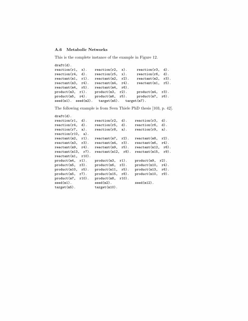
A.6 Metabolic Networks

This is the complete instance of the example in Figure 12.

draft(d).

reaction(r1, x). reaction(r2, x). reaction(r3, d).

reaction(r4, d). reaction(r5, x). reaction(r6, d).

reactant(m1, r1). reactant(m2, r2). reactant(m2, r3).

reactant(m3, r4). reactant(m4, r4). reactant(m1, r5).

reactant(m4, r5). reactant(m4, r6).

product(m3, r1). product(m3, r2). product(m4, r3).

product(m5, r4). product(m6, r5). product(m7, r6).

seed(m1). seed(m2). target(m5). target(m7).

The following example is from Sven Thiele PhD thesis [103, p. 42].

draft(d).

reaction(r1, d). reaction(r2, d). reaction(r3, d).

reaction(r4, d). reaction(r5, d). reaction(r6, d).

reaction(r7, a). reaction(r8, a). reaction(r9, a).

reaction(r10, a).

reactant(m2, r1). reactant(m7, r2). reactant(m8, r2).

reactant(m3, r3). reactant(m4, r3). reactant(m6, r4).

reactant(m9, r4). reactant(m9, r5). reactant(m12, r6).

reactant(m13, r7). reactant(m12, r8). reactant(m15, r9).

reactant(m1, r10).

product(m4, r1). product(m3, r1). product(m9, r2).

product(m5, r3). product(m6, r3). product(m10, r4).

product(m10, r5). product(m11, r5). product(m13, r6).

product(m5, r7). product(m15, r8). product(m10, r9).

product(m7, r10). product(m8, r10).

seed(m1). seed(m2). seed(m12).

target(m5). target(m10).